Sensitivity of precipitation formation to secondary ice production in winter orographic mixed-phase clouds

The discrepancy between the observed concentration of ice nucleating particles (INPs) and the ice crystal number concentration (ICNC) remains unresolved and limits our understanding of ice formation and, hence, precipitation amount, location and intensity. Enhanced ice formation through secondary ice production (SIP) could account for this discrepancy. Here, in a region over the eastern Swiss Alps, we perform sensitivity studies of additional simulated SIP processes on precipitation formation and surface precipitation intensity. The SIP processes considered include rime splintering, droplet shattering during freezing and breakup through ice–graupel collisions. We simulated the passage of a cold front at Gotschnagrat, a peak at 2281 m a.s.l. (above sea level), on 7 March 2019 with the Consortium for Small-scale Modeling (COSMO), at a 1 km horizontal grid spacing, as part of the RACLETS (Role of Aerosols and CLouds Enhanced by Topography and Snow) field campaign in the Davos region in Switzerland. The largest simulated difference in the ICNC at the surface originated from the breakup simulations. Indeed, breakup caused a 1 to 3 orders of magnitude increase in the ICNC compared to SIP from rime splintering or without SIP processes in the control simulation. The ICNCs from the collisional breakup simulations at Gotschnagrat were in best agreement with the ICNCs measured on a gondola near the surface. However, these simulations were not able to reproduce the ice crystal habits near the surface. Enhanced ICNCs from collisional breakup reduced localized regions of higher precipitation and, thereby, improved the model performance in terms of surface precipitation over the domain.

1 Introduction

Clouds consisting only of liquid droplets contribute only a small fraction to the overall precipitation on Earth (Heymsfield et al., 2020). Indeed, diffusional growth is slower for larger droplets, becoming inefficient for droplets larger than 20  µm in diameter when updraft velocities are weak (Wang, 2013). In the presence of stronger local updrafts, cloud droplets can also grow by collision–coalescence with other droplets to form raindrops. Simultaneously, the cloud droplets are transported to temperatures colder than 0 ^∘C, where they are supercooled and can freeze heterogeneously, i.e., with the aid of an ice nucleating particle (INP).

The co-existence of ice crystals and supercooled liquid water droplets in clouds plays a significant role in the formation of precipitation in the midlatitudes (Mülmenstädt et al., 2015). These clouds are known as mixed-phase clouds (MPCs) and can be found in the temperature regime between 0 to approximately −38 ^∘C (Korolev and Mazin, 2003; Morrison et al., 2012; Lohmann et al., 2016a). Several microphysical processes that may contribute to surface precipitation are unique to mixed-phase conditions. Once ice crystals exist in a supercooled liquid cloud, the cloud becomes thermodynamically unstable. Depending on the ice crystal number concentration (ICNC) and their size, an updraft of 2 m s⁻¹ may enable a MPC to sustain the simultaneous growth of ice particles and supercooled cloud droplets (Korolev, 2007). However, for lower updraft velocities, the ice crystals grow at the expense of the evaporating cloud droplets. The liquid droplets may eventually evaporate completely in the vicinity of the growing ice crystals. This process is called the Wegener–Bergeron–Findeisen process (WBF; Wegener, 1911; Bergeron, 1965; Findeisen et al., 2015) and can lead to rapid partial or full glaciation of MPCs (Blyth and Latham, 1997), e.g., when updrafts are less than 1 m s⁻¹ for an integral ice crystal radius of 10 µm cm⁻³ (Korolev, 2007). To sustain MPCs, the supersaturation with respect to water must be maintained to compete with the depletion of water vapor by the depositional growth of ice particles (Korolev and Isaac, 2002; Bühl et al., 2016). In such environments, supersaturation over liquid water is required so that cloud droplets can grow in the vicinity of ice crystals. For example, mountainous regions can provide a continuous source of liquid droplets through a constant air flow that is forced to ascend due to the topography. In the Arctic regions, MPCs can develop subcloud circulations leading to cold pool formation and updrafts driving new convective cells (Morrison et al., 2012; Lohmann et al., 2016a; Beck et al., 2018; Eirund et al., 2019a). Thus, the MPC lifetime is very sensitive to the updraft velocity (Korolev and Mazin, 2003; Lohmann et al., 2016a). Lohmann et al. (2016a) showed that high updraft velocities, induced by steep orography, can stabilize a MPC. In this case, the adiabatic cooling rate caused supersaturation with respect to liquid water to exceed the diffusional growth rate, allowing both cloud droplets and ice crystals to grow (Korolev, 2007).

Primary production of ice crystals at temperatures warmer than the homogeneous nucleation threshold temperature (−38 ^∘C) occurs through heterogeneous nucleation. The number concentration of INPs can equal the ICNC in MPCs at temperatures warmer than −38 ^∘C, when no secondary ice production (SIP) process or external ice crystal sources from the surface (e.g., hoar frost or blowing snow) or above (seeder–feeder process) are active. However, airborne observations show that the ICNC can be orders of magnitude larger than the INP concentration (Field et al., 2016, and references therein). Field campaigns conducted at Jungfraujoch, in the Bernese Alps in Switzerland, also showed that surface-based measurements of ICNC exceed INPs by several orders of magnitude (Henneberger et al., 2013; Beck et al., 2018). A modeling study conducted by Henneberg et al. (2017) over the Bernese Alps showed that simulated ICNCs during winter are underestimated by an order of magnitude in MPCs as compared to the observations taken by Lloyd et al. (2015). Temperatures were between −8 and −15 ^∘C and, therefore, too cold to trigger rime splintering, also known as the Hallett–Mossop process (Hallett and Mossop, 1974). Rime splintering occurs at warmer subzero temperatures, between −3 and −8 ^∘C, and dominates ice multiplication in the early stages of the cloud's existence. However, a cold cloud base leads to slower diffusional droplet growth. In this case, the cloud droplets remain smaller than the required 24 µm in diameter that is needed for multiplication through rime splintering (Hallett and Mossop, 1974). This cold cloud base could dampen the immense multiplicative nature of rime splintering, revealing the dominance of other possible mechanisms for multiplication early in a cloud's existence, for example, the collisional breakup of ice particles (Yano and Phillips, 2011). The collisional breakup of ice particles is a result of the collisional kinetic energy and was found to be most active at −15 ^∘C. Vardiman (1978) showed that collisional breakup occurs when large concentrations of rimed ice crystals are present in convective clouds, which increases SIP significantly.

Numerical formulations have been developed to describe SIP by the collision of different ice species (e.g., Phillips et al., 2017a), e.g., when graupel collides with ice crystals, when ice crystals collide with snow (e.g., Yano and Phillips, 2011; Sullivan et al., 2018a) or when larger graupel collides with smaller graupel (Sullivan et al., 2017, 2018b; Sotiropoulou et al., 2020). Therefore, the mass concentrations of the collider species must be adequately simulated (e.g., Otkin et al., 2006), as any misrepresentation in the graupel category could potentially lead to significant differences in the SIP rate. There are, however, only a small number of studies that have used these collisional breakup parameterizations in mesoscale models (e.g., Sullivan et al., 2018a; Hoarau et al., 2018; Sotiropoulou et al., 2020). Notably, Sullivan et al. (2018a) demonstrated that the lack of graupel formation in a cold frontal rainband in numerical simulations compared to observations (Crosier et al., 2014) caused collisional breakup to be 2 orders of magnitude less effective in SIP compared to rime splintering. Graupel was the only ice species that could cause collisional breakup when it collided with either ice crystals or snowflakes. Another possibility for SIP is droplet shattering upon freezing (e.g., Kolomeychuk et al., 1975; Lauber et al., 2018). If the pressure within a droplet reaches a critical point, the droplet may fragment upon freezing. This process has been observed to happen for droplets larger than about 40 µm in diameter (e.g., Lawson et al., 2015; Korolev et al., 2020). The likelihood of fragmentation upon freezing and the number of produced splinters during the fragmentation increases with droplet size (Kolomeychuk et al., 1975; Lauber et al., 2018, 2021). In a modeling study, Sullivan et al. (2018b) showed that a warm cloud base, between 20 and 25 ^∘C, at an updraft velocity of 4 m s ⁻¹, is required for cloud droplets to grow large enough through coalescence or condensation to freeze and then shatter. As the cloud base temperature and updraft velocity decrease, droplet shattering becomes less efficient. Sullivan et al. (2018a) could address the discrepancy between ICNC and INP concentrations in their simulations by using the rime splintering, collisional breakup and droplet shattering processes simultaneously.

Several other mechanisms like hoar frost and blowing snow have been suggested as being surface flux processes that could lift ice particles from the surface of mountains and increase the ICNC of winter orographic MPCs (Rogers and Vali, 1987; Farrington et al., 2016; Beck et al., 2018). Farrington et al. (2016) simulated ICNC at Jungfraujoch with a simplified parameterization for hoar frost. However, this parameterization is independent of the surface concentrations of hoar crystals, and including temporal variations in these surface concentrations could improve the parameterization accuracy (Farrington et al., 2016). ICNC enhancement due to hoar frost and blowing snow could also aid in enhancing further SIP processes, but, currently, it is unknown which of these processes dominates under different conditions. Understanding and representing the ICNC through the cloud, and not only at the base of the cloud due to surface processes, can also aid in obtaining a better representation of the surface shortwave budget, particularly in the Antarctic (Young et al., 2019). Independent of surface processes, hoar frost and blowing snow, we are investigating the discrepancy between ICNC and INP concentrations from the perspective of SIP to examine two points. First, how active SIP processes are in wintertime orographic MPCs, and whether they could explain the observed ICNC in a case study of the RACLETS (Role of Aerosols and CLouds Enhanced by Topography and Snow) field campaign. Second, what is the effect of SIP processes on the cloud microphysics and, consequently, precipitation formation, location and intensity?

2 Methods

2.1 Case study of the RACLETS field campaign

The RACLETS campaign took place in February and March 2019 in the Davos region in Switzerland (also discussed in more detail in Lauber et al., 2021, and Ramelli et al., 2021a, b). Its goal was to improve our understanding of the influence of both orography and aerosols on the development of clouds and on precipitation formation. Of particular interest is that a cold front passed over the Swiss Alpine region on 7 March 2019 and was captured by measurements of precipitation and in situ measurements of cloud droplets, ice crystals and INPs. The precipitation rate and liquid water path (LWP) data were provided by the Leibniz Institute for Tropospheric Research (TROPOS). The precipitation rate was collected from rain gauge data when available, and otherwise from an upward pointing radar situated at Davos Wolfgang, 1630 m a.s.l. (above sea level) at a temporal resolution of 30 s. However, the radar attenuation from 08:15 to 14:00 UTC was not corrected for. As a result, no estimation of supercooled liquid within the MPC could be made. The LWP was estimated by the microwave radiometer that was situated at the same location as the radar. We also used the precipitation data from MeteoSwiss in the form of a CombiPrecip product, which is computed using a geostatistical combination of radar estimates from plan position indicator radar data with rain gauge measurements (Sideris et al., 2014). We used CombiPrecip to capture the spatial extent of precipitation over the Swiss Alps at an hourly resolution.

Furthermore, ice crystal properties were collected using the HoloGondel platform installed on the Gotschnabahn (described in Lauber et al., 2021), which consists mainly of the HOLographic Imager for Microscopic Objects 3G (HOLIMO 3G in Beck et al., 2017). The outcome product of HOLIMO 3G is 2D images of cloud particles, which can be differentiated in ice and liquid particles for particles larger than 25 µm, depending on the shape of the ice particles (Henneberger et al., 2013). The separation between liquid droplets and ice crystals was done with a fine-tuned version of the neural network described in Touloupas et al. (2020), with an overall uncertainty of the ICNC of ±10 %. Above that, the ice crystals were manually classified into irregular, pristine, rimed and aggregated particles, which provides valuable information on the precipitation formation process in orographic MPCs. Note that ice crystals can also be rimed aggregates and, thus, fall into two categories. Because of the total small number of recorded ice crystals and their different categories, the counting uncertainty ($\sqrt{N}/V$; N – number of crystals; V – measurement volume) was added to the overall uncertainty for the ICNC and for the different categories.

HoloGondel was installed on a cable car on the Gotschnabahn, which runs on the northwestern side of the ridge towards Gotschnagrat (2281 m a.s.l.), north of Davos Wolfgang (see Fig. 1 for the exact location). HoloGondel took in situ images of ice crystals and droplets within the cloud during three separate ascents of the Gotschnabahn running at the upper section between Gotschnaboden (1790 m) and the Gotschnagrat mountain station (2280 m), specifically at 11:54, 12:54 and 13:26 UTC on 7 March 2019. During these times, temperatures ranged between −2.8 and 0.7 ^∘C between Gotschnaboden and Gotschnagrat.

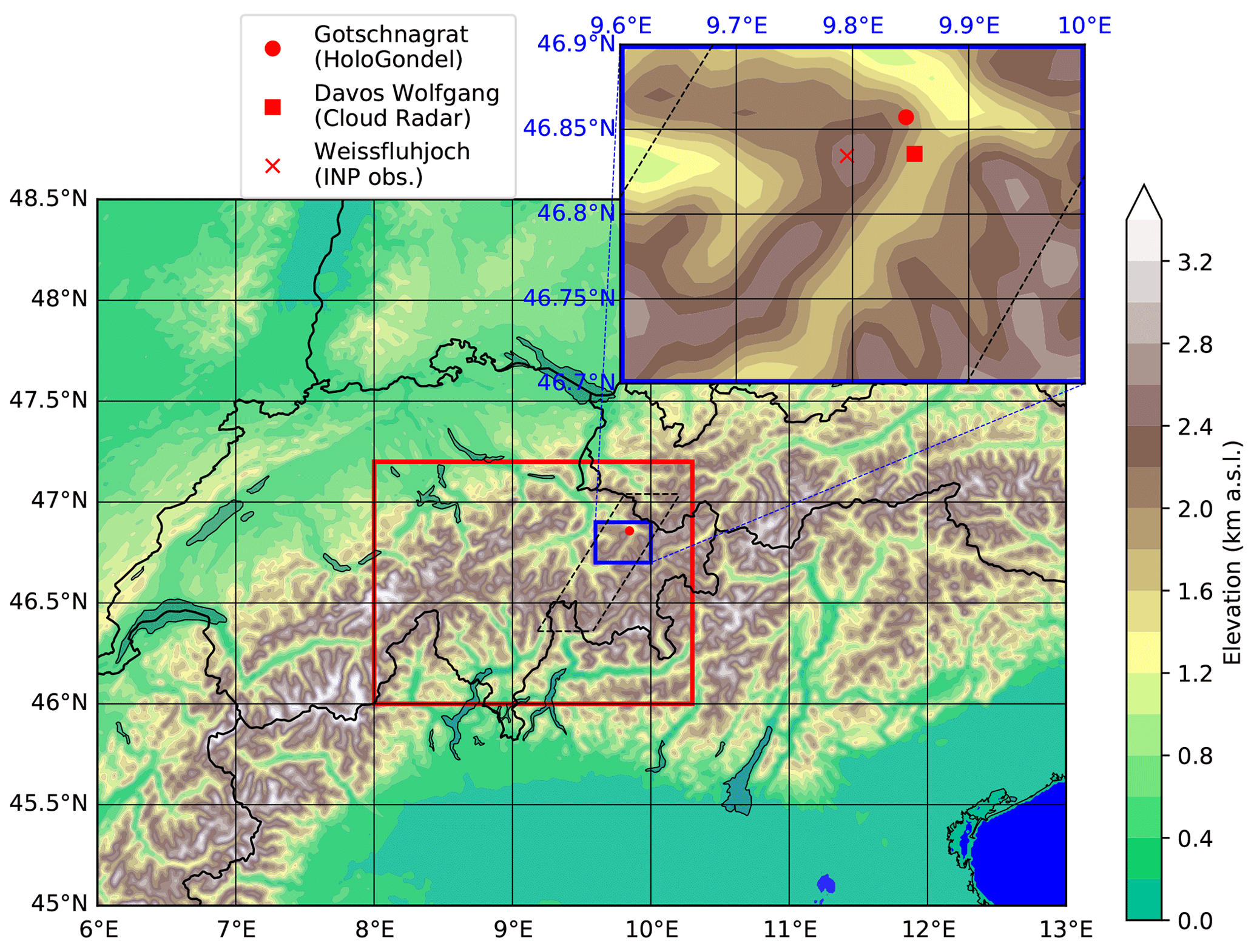
Figure 1 Overview of the model orography and the instrument location setup. The large domain is the simulated area that contains the analysis domain (red box). The enlarged blue domain is the location where measurements were taken during the RACLETS campaign. The parallelogram (dashed black lines) is the domain of the flow-oriented vertical cross section.

2.2 Model setup

2.2.1 Spatial and temporal resolution

For the purposes of better understanding precipitation formation, we used the non-hydrostatic limited-area atmospheric model of the Consortium for Small-scale Modeling (COSMO; Baldauf et al., 2011) version 5.4.1b. COSMO has recently been used to study wintertime orographic MPCs in the Swiss Alps (Lohmann et al., 2016a; Henneberg et al., 2017). The model domain roughly covers a region of 500 km × 400 km (45.5 to 49.5^∘ N and 6 to 13^∘ E) at a horizontal grid spacing of 1.1 km×1.1 km (Fig. 1). For reference, Davos Wolfgang is situated at 46.835^∘ N and 9.85^∘ E. A height-based hybrid smoothed level vertical coordinate system (Schär et al., 2002) with 80 levels was used and stretched from the surface to 22 km. The applied orographic smoothing at a horizontal resolution of 1.1 km×1.1 km reduces the elevation of Gotschnagrat (located at 2300 m a.s.l.) to 1880 m a.s.l. For this study, we simulate the cold front passage between 07:00 and 14:45 UTC and analyze the results between 09:30 and 14:45 UTC on 7 March 2019. Hourly initial and boundary conditions analysis data at a horizontal resolution of 7 km × 7 km, supplied by MeteoSwiss, were used to force COSMO. The model time step was 4 s and the output frequency every 15 min.

Simulations were conducted with the SIP processes, where several SIP processes were active at the same time, and a control simulation (CNTL), where none of the SIP processes was active. For each of these simulations, five ensemble simulations are conducted by perturbing the initial temperature conditions at each grid point through the model domain with unbiased Gaussian noise at a zero mean and a standard deviation of 0.01 K (Selz and Craig, 2015; Keil et al., 2019).

2.2.2 Cloud microphysics scheme

We use a detailed two-moment bulk cloud microphysics scheme within COSMO with six hydrometeor categories, including hail, graupel, snow, ice, raindrops and cloud droplets (Seifert and Beheng, 2006). The two-moment bulk microphysics scheme has been used extensively to study the evolution, lifetime, persistence and aerosol–cloud interactions of MPCs (Seifert et al., 2006; Baldauf et al., 2011; Possner et al., 2016; Lohmann et al., 2016a; Possner et al., 2017; Henneberg, 2017; Glassmeier and Lohmann, 2018; Sullivan et al., 2018a; Eirund et al., 2019a, b). We refer to ice particles as any combination of the hail, graupel, snow or ice categories. The size distributions of the hydrometeors, except for the raindrop category which is described by an exponential distribution, are described by a generalized gamma distribution. Cloud droplet activation is based on an empirical activation spectrum which depends on the cloud base vertical velocity and the prescribed number concentration of cloud condensation nuclei (Seifert and Beheng, 2006). The application is appropriate in atmospheric models with a horizontal grid size and time resolution of Δx≤1 km and Δt<10 s respectively. Condensation and evaporation, represented by a saturation adjustment approach, are applied after the microphysical conversion rates. The warm-phase autoconversion process from Seifert and Beheng (2001) was updated with the collision efficiencies from Pinsky et al. (2001) and also takes into account the decrease in terminal fall velocity associated with an increase in air density. A better approximation of the collision rate between hydrometeors was also introduced by Seifert and Beheng (2006), which makes use of the root mean square values instead of the absolute mean values of the difference between the fall velocity of the colliding hydrometeors from the Wisner approximation (Wisner et al., 1972).

INPs available for immersion freezing are prognostic throughout the simulations and are implemented following Possner et al. (2017) and Eirund et al. (2019b). The immersion freezing parameterization follows the DeMott et al. (2015) temperature dependence and reproduces the depletion and replenishment of INPs. The initial aerosol concentration for particles larger than 0.5 µm in diameter required for estimating the INP concentration was measured at Weissfluhjoch (2670 m a.s.l.) in clear air condition between 08:00 and 08:58 UTC on 5 March 2019. The days following 5 until 7 March were cloudy, and an INP concentration was not measured. The average aerosol concentration larger than 0.5 µm during this time was 3.32 cm⁻³ at an ambient air temperature of 261 K (Seifert, 2019). Because of the temperature mismatch between the observed temperature and the temperature range for which the INP parameterization is accurate (T<258, DeMott et al., 2010), we used the retrieved aerosol concentration from the upward-pointing lidar that was situated at Davos Wolfgang. The lidar retrieval gave a full vertical profile of the atmosphere. At temperatures between 258 and 243 K, the aerosol concentration larger than 0.5 µm was between 1.8 and 2.5 cm⁻³ for which we then, accordingly, chose 2 cm⁻³ as input for the DeMott et al. (2015) parameterization. At a temperature of 243 K, the estimated INP concentration was 23 L⁻¹. The freezing of all cloud droplets occurs at temperatures colder than 223 K. The homogeneous freezing of cloud droplets, which is strongly dependent on temperature, occurs at warmer subzero temperatures. Another pathway of the liquid-to-ice conversion is the homogeneous nucleation of solution droplets that are typically associated with cirrus cloud formation. The formulation of the homogeneous nucleation of solution droplets follows Kärcher et al. (2006), which determines the number density and size of nucleated ice crystals as a function of vertical wind speed, temperature and pre-existing cloud ice. A critical supersaturation must be reached in which nucleation events can occur if the updraft is stronger than a threshold value determined by the radius and number density of the pre-existing ice crystals (Eq. 19 of Kärcher et al., 2006). The freezing of raindrops occurs heterogeneously and independently of INPs. This is because the raindrop number concentration is at least a factor of 10³ smaller than the cloud droplet number concentration and has an insignificant contribution to the primary production of ice upon freezing (Figs. S4 and S5i and j). It is included in our simulations because it is needed for droplet shattering to occur. In the spectral partitioning of freezing rain, only the frozen raindrops that are partitioned as ice (Blahak, 2008) can cause multiplication through droplet shattering, as discussed in the following section.

2.2.3 Secondary ice production parameterizations

Besides the primary ice formation pathways through homogeneous and heterogeneous nucleation, rime splintering is the only process included in the standard version of COSMO that can enhance the ICNC otherwise. The rime-splintering process has been parameterized, implemented and tested in numerical weather models (Blyth and Latham, 1997; Ovtchinnikov and Kogan, 2000; Phillips et al., 2006; Milbrandt and Morrison, 2016; Phillips et al., 2017a). In COSMO, rime splintering occurs exclusively after collisions between supercooled cloud droplets of diameter greater than 25 µm or raindrops with ice, snow, graupel or hail, all larger than 100 µm (e.g., Seifert and Beheng, 2006), at temperatures between −3 and −8 ^∘C (Hallett and Mossop, 1974). The predominant theory is that, within this temperature range, the supercooled droplets that rime on large ice particle freeze resulting in a buildup of internal pressure whereby the pressure is relieved when the frozen shell cracks and produces 3.5×10⁸ per kilogram of rime secondary ice particles (Hallett and Mossop, 1974). At temperatures colder than −8 ^∘C, the ice shell of the frozen droplet is too strong to break (Griggs and Choularton, 1983), and at warmer temperatures than −3 ^∘C, the supercooled droplet spread over the ice particle did not cause any SIP (Dong and Hallett, 1989). However, SIP has also been observed at temperatures outside the Hallett–Mossop droplet size and temperature requirements.

Droplet shattering produces maximum splinters at around −15 ^∘C when large droplets freeze and shatter if the internal pressure buildup is high enough to eject fragments (e.g., Kolomeychuk et al., 1975; Leisner et al., 2014; Wildeman et al., 2017; Lauber et al., 2018; Keinert et al., 2020). So far, no temperature constraint is known for this process to be active below 0 ^∘C (Korolev et al., 2020; Lauber et al., 2021). The pressure buildup occurs mainly due to the unique characteristic of liquid water having a higher density than ice and, thus, expanding when it freezes. Larger droplets are more likely to shatter and likely produce more ice splinters (Kolomeychuk et al., 1975; Lauber et al., 2018). However, as of yet, the number of splinters that are produced during droplet shattering could not be quantified. A more rigorous formulation for the fragment number remains a challenge due to the lack of measurement in laboratory studies. Lauber et al. (2018) showed that the highest fragment rates occur at around −15 ^∘C; however, this was only for droplet sizes of 83 and 310 µm. Droplet shattering in COSMO is parameterized as the product of a fixed fragment number, a temperature-dependent shattering probability given by a normal distribution in temperature and the existing raindrop freezing tendency used by Seifert and Beheng (2006). The normal distribution is centered at 258 K, with a standard deviation of 5 K and a maximum probability of 10 % (as illustrated in Fig. 2a).

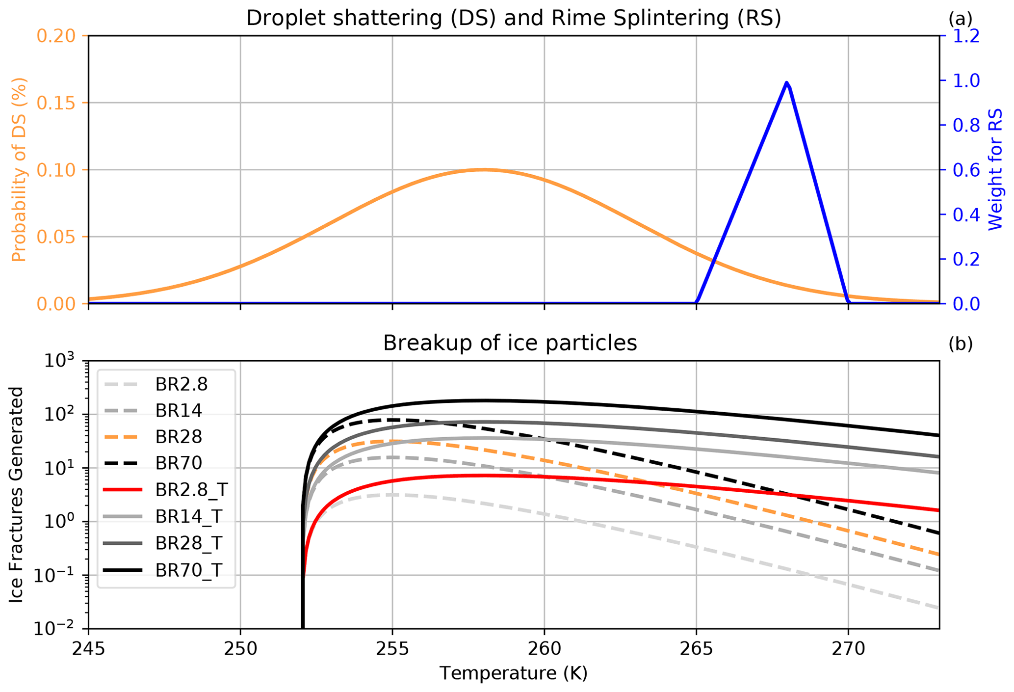
Figure 2 Secondary ice production processes at their defined temperature ranges. Panel (a) shows the probability of occurrence of droplet shattering (DS) and the triangular weighting function of rime splintering (RS). Panel (b) shows the fragment numbers generated by ice–graupel collisional breakup (BR) for the different cases shown in Table 1. The red and yellow lines in (b) are the collisional breakup parameterizations that were analyzed in the results.

The collisional breakup of ice particles, in ice–ice collisions, was introduced and studied in laboratory experiments by Vardiman (1978) and Takahashi et al. (1995) and found to be most effective at −15 ^∘C. Takahashi et al. (1995) enforced the collision of large, 1.8 cm in diameter, heavily rimed ice particles with one another and generated secondary ice particles of up to 10³ per collision. Yano and Phillips (2011) and Yano et al. (2016) have demonstrated the generation of massive enhancement of the ICNC by SIP due to ice–ice collision in a dynamical system-type model. Recently, Phillips et al. (2017a) developed a more physically robust theoretical parameterization that was also applied in numerical simulations that consider energy conservation. In our case, following Sullivan et al. (2018a), we take a more simplified approach. The collisional breakup of ice particles in the laboratory work of Takahashi et al. (1995) resulted in a temperature-dependent parameterization of the fragment number, as follows:

$$\begin{array}{}\text{(1)}& {\displaystyle }& {\displaystyle }{\mathrm{\aleph }}_{\mathrm{BR}}={\displaystyle \frac{F_{\mathrm{BR}}}{\mathit{\alpha }}}(T-\mathrm{252}{)}^{\mathrm{1.2}}\exp \left[\begin{array}{c}-(T-\mathrm{252})/{\mathit{\gamma }}_{\mathrm{BR}}\end{array}\right],\text{(2)}& {\displaystyle }& {\displaystyle }{\left.\begin{array}{c}\frac{\partial N_{\mathrm{ice}}}{\partial t}\end{array}\right|}_{\mathrm{BR}}=-{\mathrm{\aleph }}_{\mathrm{BR}}{\left.\begin{array}{c}\frac{\partial N_j}{\partial t}\end{array}\right|}_{\mathrm{coll},jk},\end{array}$$

where α is the scale factor, F_BR is the leading coefficient, T is the temperature in Kelvin, and γ_BR is the decay rate of fragment number at warmer temperatures. In our breakup simulations, F_BR and γ_BR are the experimental factors that are adapted for evaluating the collisional breakup parameterization. The fragment number ℵ_BR is multiplied by the collisional tendency $\partial N_j/\partial t$ of the colliding hydrometeor pairs to calculate the number of ice generated per time step $\partial N_{\mathrm{ice}}/\partial t$ in Eq. (2). As shown in Fig. 2b, no collisional breakup occurs for temperatures below 252 K. Takahashi et al. (1995) forced the collision between heavily rimed ice particles at a velocity of 4 m s⁻¹. However, when the collision speed from the experiment is used to calculate the size of the involved graupel particles, a 4 m s⁻¹ fall speed corresponds to graupel particles in the range of 2.5 mm in diameter according to Lohmann et al. (2016b). Considering the size–mass and fall–mass relations that are used in COSMO, Blahak (2008) showed that, for graupel and hail falling at 4 m s⁻¹, the effective diameters were 4 mm and 1.4 mm, respectively. Also, in the simulations conducted here, graupel sizes would very rarely exceed 3 mm in diameter (not shown here). Therefore, having smaller graupel particles than what was used in Takahashi et al. (1995), we expect ℵ_BR to be less, and thus, we introduce α to prevent extreme overestimations in ℵ_BR (Table 1). In contrast to Sullivan et al. (2018b, Table 1), graupel was the only species that could collide with and break up ice or snow. Therefore, in our collisional breakup simulations, hail was not permitted to collide with graupel and so reduce the graupel diameter to smaller sizes, which emphasizes the need for α. Another consideration to take into account is that COSMO treats snowflakes as unrimed particles, and as soon as riming occurs on snowflakes, the snow mixing ratio is converted to the graupel mixing ratio, causing an especially large graupel mixing ratio (Otkin et al., 2006). Since graupel is the only contributor to SIP through collisional breakup, increased graupel mixing ratios could lead to excessive SIP. Further sensitivity studies were conducted with γ_BR of 2.5 instead of 5 as described in the parameterization used by Sullivan et al. (2018a). When γ_BR is 2.5, ℵ_BR will be reduced at warmer temperatures (Fig. 2b).

Table 1 Sensitivity settings for the collisional breakup parameterization. α is the scale factor, F_BR the fragments generated and γ_BR the decay rate of the fragment number at warmer temperatures. Shown in bold is γ_BR=5, as used by Sullivan et al. (2018a).

In the standard version of COSMO, the ICNC after each model time step is limited to 500 L⁻¹ for each level. However, measurements showed that the ICNC within MPCs produced higher ICNC of up to 1014 L⁻¹ (Lohmann et al., 2016a). Korolev et al. (2020) identified midlatitude frontal cloud systems within a temperature range of −15 and 0 ^∘C to have 500 to 1000 L⁻¹ small faceted ice crystals. Therefore, we increased the ICNC limit to 2000 L⁻¹ in our model setup.

Using droplet shattering as the only active SIP process in our case study yields very similar results to the CNTL simulations, with the exception that the SIP rate between 4 and 5 km was 0.01 L⁻¹ s⁻¹. The low SIP rate by droplet shattering is because of the small rain mixing ratio at the needed temperatures for this process. Therefore, it was not included in the rest of our analysis (Fig. S1 in the Supplement). Also, the initial analysis of the simulations with collisional breakup (for γ_BR=2.5) showed that the SIP rate is between $\mathrm{1}\times {\mathrm{10}}^{-\mathrm{3}}$ and 7 L⁻¹s⁻¹ below 5 km, yielding an ICNC between 0.1 and 300 L⁻¹ at the surface (Fig. S2a and g). Contrasted against these simulations are the collisional breakup simulations (for γ_BR=5) that showed an increased SIP rate between 100 and 1000 L⁻¹ s⁻¹, yielding ICNC of 2000 L⁻¹ at the surface at Gotschnagrat (Fig. S3a and g). However, the ICNCs were strongly influenced by the upper bound of the ICNC in COSMO, especially between 3 and 5 km. We chose the BR2.8_T settings because the observed ICNC was reproduced best near the surface at Gotschnagrat in this simulation. Furthermore, the ICNC hard limit did not impact the simulations, and therefore, collisional breakup and its impacts on the MPC can be understood better. Furthermore, we used the BR28 simulation as a comparison to understand what the effect would be by reducing the SIP at warmer temperatures than 263.5 K, while at the same time increasing the SIP at colder temperatures than 263.5 K compared to the BR2.8_T settings (Fig. 2b). Higher ice particle number concentrations at colder temperatures can increase the competition for available cloud liquid water and glaciate the clouds at a faster rate, slowing down precipitation formation. Due to their smaller size as a result of the aggressive collisional breakup, these ice particles should have slower sedimentation velocities. We do expect that precipitation formation will be slower in the BR28 simulations, and that there will be a leeward shift in surface precipitation, assuming that the lower part of the MPC is supersaturated with respect to water.

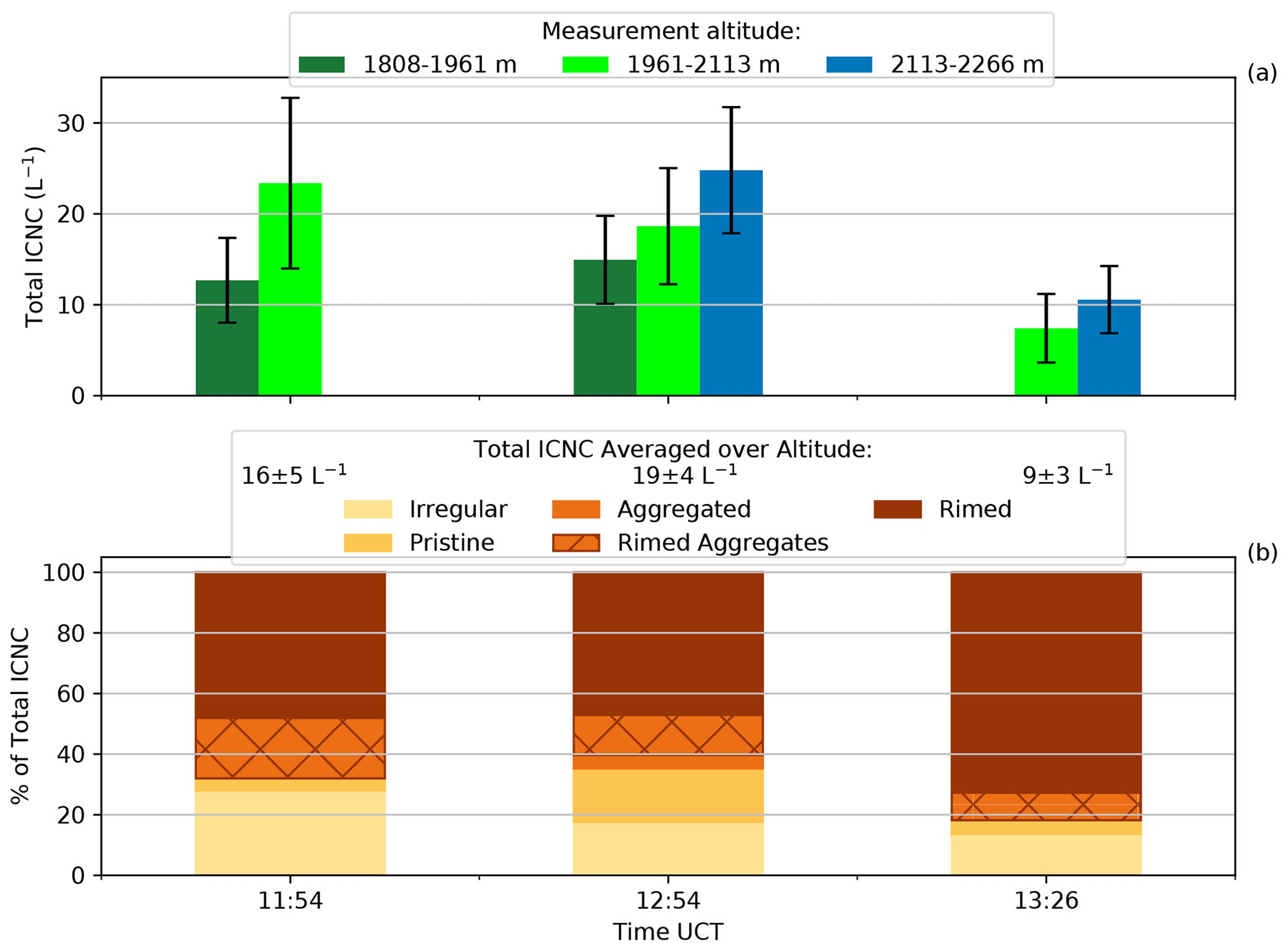
Figure 3 HoloGondel measurements on 7 March 2019. (a) Total ICNC and measurement uncertainty (black error bars) of each gondola run at each altitude. No measurements were taken at 11:54 UTC between 2113–2266 m and at 13:26 UTC between 1808–1961 m. (b) Irregular, pristine, aggregated, rimed and rimed aggregate ice particles as the percentage of total ICNC averaged over the altitudes of each gondola run are shown. The median temperature for each of the rides at the respective height, 1808–1961, 1961–2113 and 2113–2266 m, corresponds to −1, −1.5 and −2.5 ^∘C, respectively.

3 Results

3.1 Modeling ICNC and ice growth rates at Gotschnagrat

3.1.1 Modeling ICNC

During each ∼2 min ascent, the HoloGondel platform on the cable car recorded ice crystal concentrations averaged over three altitudes (1808–1961, 1961–2113 and 2113–2266 m). We first show the ICNC inferred from HoloGondel measurements on each of its three ascents (at 11:54, 12:54 and 13:26 UTC) and as the outcome of COSMO simulations at Gotschnagrat (Fig. 1a). The total ICNCs from the observations were averaged over altitude for each ascent and were 16±5, 19±4 and 9±3 L⁻¹ at 11:54, 12:54 and 13:26 UTC, respectively. The simulated ICNC from the CNTL and rime-splintering simulations was less than 0.1 L⁻¹ below 2.15 km for both 12:00 and 13:00 UTC (Figs. 4 and 5a) and was at least 2 orders of magnitude smaller than the observations at Gotschnagrat (Fig. 3). Between 2.2 and 3.2 km, the SIP rate from rime splintering reached $\mathrm{5}\times {\mathrm{10}}^{-\mathrm{3}}$ L⁻¹ s⁻¹ (Figs. 4 and 5g). Rime splintering originated exclusively from raindrops, with diameters between 150 and 250 µm at a concentration of 0.1 L⁻¹ that rimed onto ice particles (Fig. S4e and o). A diameter of 25 µm required for rime splintering to be active was not met by the cloud droplets, which only reached diameters of 20 µm (Figs. 4 and 5f). The CNTL and rime-splintering simulations reached cloud droplet number concentrations of 100 cm⁻³ and droplet diameters between 10 and 22 µm, aiding in the primary ice production. The underestimated ICNC by the CNTL and rime-splintering simulations emphasized the need to explore SIP with collisional breakup.

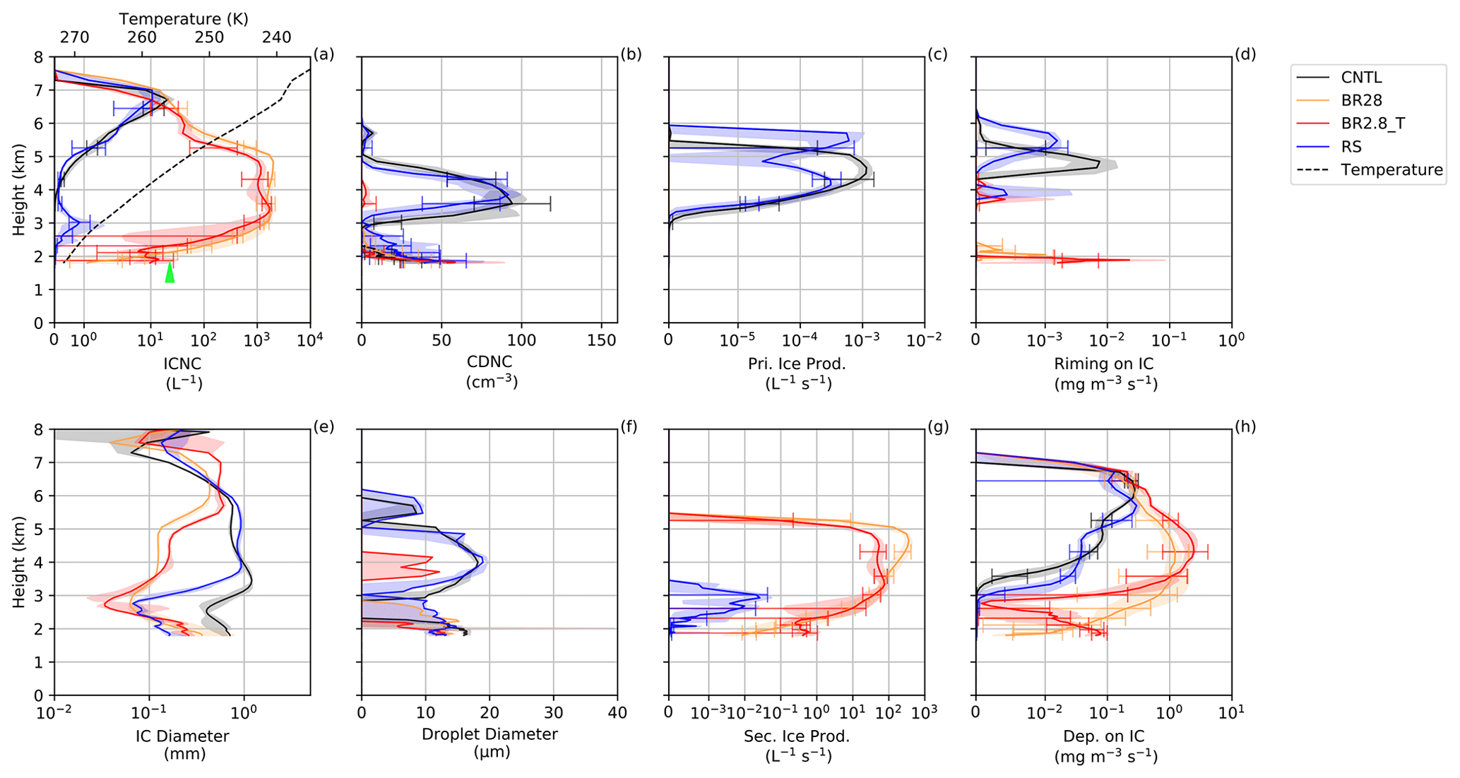
Figure 4 (a, e) Ice crystal number concentration (ICNC) and diameter, (b, f) cloud droplet number concentration (CDNC) and diameter, (c, g) primary and secondary ice production and (d, h) riming and depositional (Dep.) growth of ice at Gotschnagrat at 12:00 UTC. The solid lines are the model mean, with error bars showing the model spread for each simulation. The shaded regions are the minimum and maximum values for the four closest model points. The mean ice diameter is denoted by IC. The green arrow is the average ICNCs from the HoloGondel measurements (Fig. 3a).

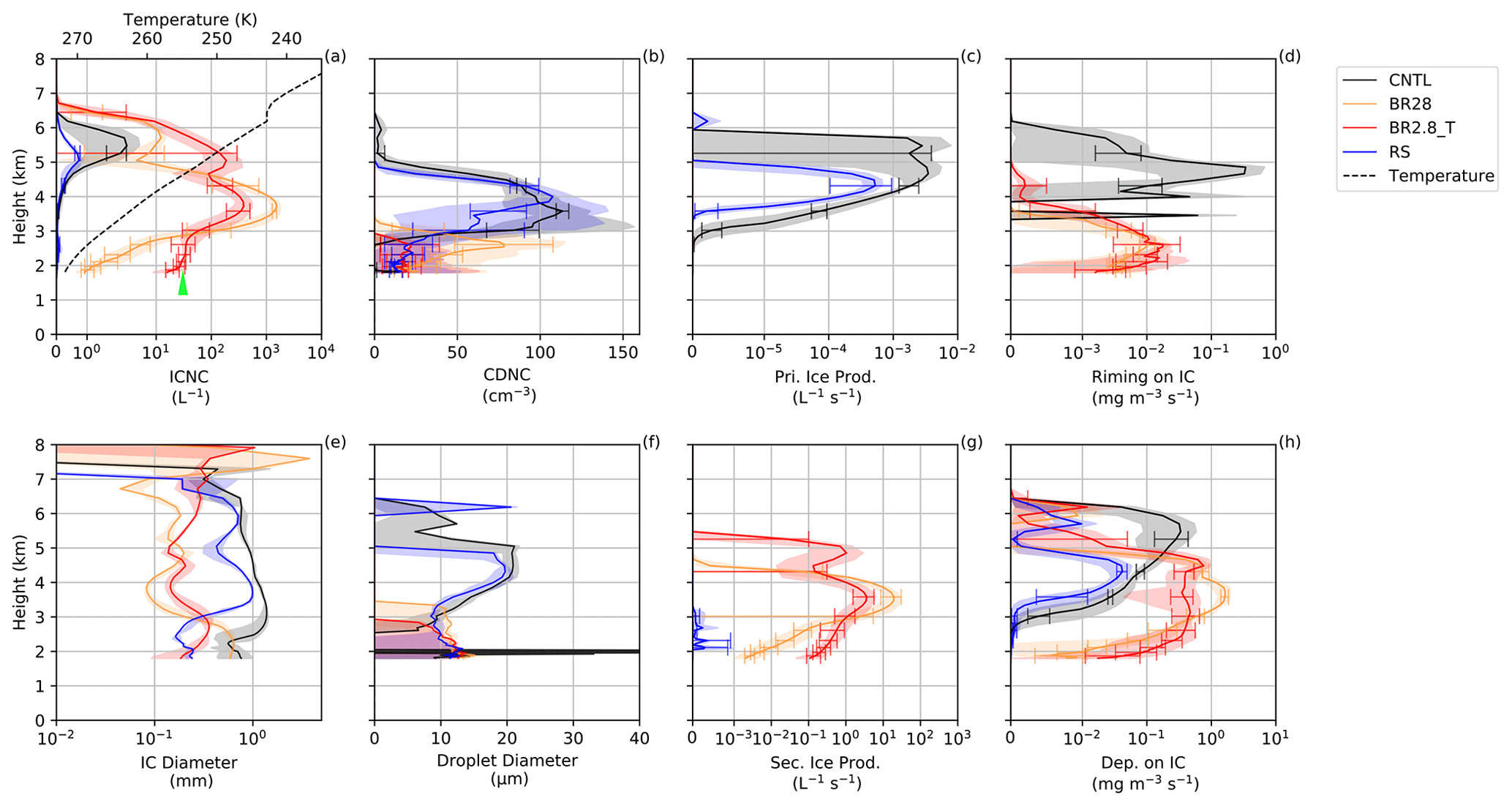
Figure 5 (a, e) Ice crystal number concentration (ICNC) and diameter, (b, f) cloud droplet number concentration (CDNC) and size, (c, g) primary and secondary ice production and (d, h) riming and depositional (Dep.) growth of ice at Gotschnagrat at 13:00 UTC. The solid lines are the model mean, with error bars showing the model spread for each simulation. The shaded regions are the minimum and maximum values for the four closest model points. The mean ice diameter is denoted by IC. The green arrow is the average ICNCs from the HoloGondel measurements (Fig. 3a).

The ICNC in the BR28 simulation, with reduced ice fracture generation at warmer subzero temperatures, was between 1 and 2 L⁻¹ at 12:00 and 13:00 UTC (Figs. 4 and 5a), within an order of magnitude of the HoloGondel observations. The ICNC from the BR2.8_T was higher between 10 and 12 L⁻¹, which compared better to the HoloGondel observations, albeit with a high uncertainty below 3 km at 12:00 UTC. Differences in the ICNC profiles and specifically at the surface are to be expected between BR28 and BR2.8_T because γ_BR controls the vertical ICNC profile. However, in Fig. 4, there is a sharp decrease in the ice and snow mixing ratio, the depositional and riming rate and the cloud liquid between 2 and 3 km in altitude in the BR2.8_T simulation. It is likely that there was an inhomogeneity in the MPC, acting as a sink to the mixing ratios and number concentrations and affecting the collisional tendencies and secondary ice production rates. The SIP rate of collisional breakup was 2 orders of magnitude larger than rime splintering for 265 K $\le T\le \mathrm{270}$ K. The ICNC from collisional breakup was significantly larger than the CNTL simulation above 3 km. This process resulted in lower liquid water and rain mass mixing ratios, preventing primary ice production because of the absence of liquid water (Figs. 4 and 5a–c and g).

3.1.2 Modeling ice growth rates

The enhanced SIP through collisional breakup had a significant impact on mostly glaciating the cloud above 2.5 km and can be seen in the nearly non-existent primary ice production rates due to the lack of cloud droplets (Fig. 4b and c). This also meant that the growth of ice was mostly through vapor deposition that, in turn, suggests that the ice was mostly unrimed and belongs in the irregular or pristine categories above 2.5 km (Fig. 4d and h). Below 2.5 km, a very shallow liquid layer that was subsaturated with respect to liquid water was present, causing ice particles to grow through the WBF process and/or riming at 12:00 and 13:00 UTC (Figs. 4, 5a, b, d, f and S4d and e). The shallow mixed-phase cloud layer was of interest because, close to the surface the HoloGondel, observations showed that rimed particles were dominant, making up 47 %–72 % of the total ICNC, indicating that the cloud (at least close to the surface), from 11:54 to 13:26 UTC, was in a mixed-phase state while passing over Gotschnagrat (Fig. 3b). Surprisingly, the rime-splintering simulation contributed little towards SIP, considering the large fraction of observed rimed particles (Figs. 3b, 4 and 5g). There are two possibilities for this discrepancy. First, from the observations, the possibility exists that the recirculation of raindrops occurred, leading to additional breakup (Lauber et al., 2021). Ice particles that fall through the melting layer (∼1500 m; −1 ^∘C at 1808–1961 m; Fig. 3 caption) and melt to raindrops are lifted back into the MPC by the turbulent mountainous flow. The increased in situ rain mixing ratio can provide additional rimer and, therefore, increase the number of rimed ice particles. Second, the low SIP rate can be attributed to the lack of available liquid water in general, and when cloud droplets were present, they were too small (less than 25 µm) to initiate rime splintering (Hallett and Mossop, 1974). From the holographic images giving information on the ice particle size and habit, the precipitation-forming processes can be inferred (Fig. 3a and b). Interestingly, observed irregularly shaped ice crystals were also present that could have been artifacts from the collisional breakup of ice or snow. However, it is also possible that the irregular ice crystals could either have originated from ice crystals that fell through different growth regimes, or they were from blowing snow and cannot be assigned to a specific group (e.g., SIP). This would mean that only a fraction of the irregular ice crystals originated from the collisional breakup.

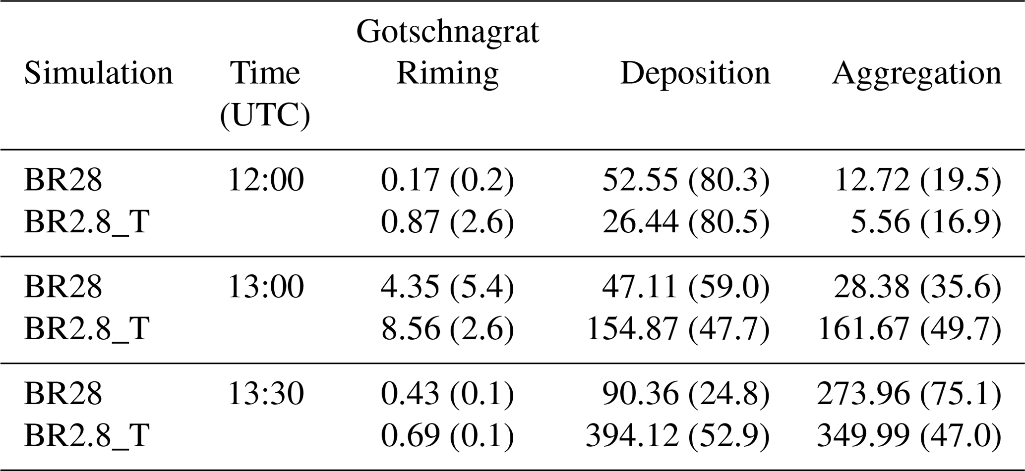
Considering the lowest 700 m in the model, we calculated the growth fraction of each of the growth mechanisms (riming, deposition and aggregation) of ice (e.g., riming (percent) = riming/(riming + deposition + aggregation) from Table 2). This was done to compare the ice crystal classification to the HoloGondel observations. This was not meant to be a direct comparison because the ice in the model could be rimed while also growing further by deposition, and vice versa, that could lead to double counting of processes. However, following this approach, the BR2.8_T simulation showed that 2.6 %, 80.5 % and 16.9 % of the growth was by riming, deposition and aggregation, respectively, at 12:00 UTC, compared to the BR28 simulation which showed growth fractions of 0.2 %, 80.3 % and 19.5 %. At 13:00 and 13:30 UTC, the collisional breakup simulations experienced growth by riming of below 5.4 %, suggesting that most of the ice would have been either pristine or aggregated, whereas the ice crystal observations were predominantly rimed in the observations. Evidently, the cloud liquid water that acts as rimers is underestimated in the collisional breakup simulations. This analysis of the results could not be carried over to the CNTL and rime-splintering simulations due to the underestimated ICNC. The ice that formed through primary ice production above 3 km sedimented through the overestimated liquid layer (Fig. 6b) and grew by deposition and riming (acting as a stronger sink to the ICNC), resulting in higher conversion rates from ice to graupel (Figs. 4 and 5b–d and h).

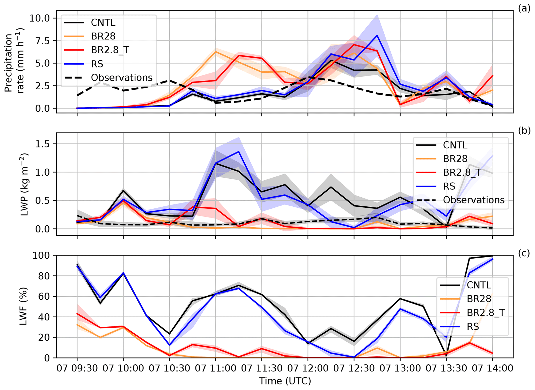
Figure 6 Time series of (a) the precipitation rate from the rain gauge and cloud radar and (b) LWP from the microwave radiometer are compared to all the sensitivity simulations at Davos Wolfgang. We interpolated the precipitation rate, LWP and LWF (liquid water fraction) from the four closest model grid points to Davos Wolfgang. The shaded areas show the model spread for each simulation. Panel (c) shows the LWF (percent) from 09:30 to 14:00 UTC on 7 March 2019. The observations, with their 30 s frequency, are integrated over 15 min intervals. The model precipitation is accumulated over every 15 min.

Table 2 Vertically integrated growth rates (milligrams per square meter per second; hereafter mg m⁻² s⁻¹) of ice over the lowest 700 m at Gotschnagrat. In parentheses are the corresponding growth rate percentages.

3.2 Modeling precipitation

To analyze the impact of ICNC on precipitation, we compared the cloud radar precipitation rate and the LWP from the microwave radiometer with that of the simulated precipitation rate and LWP. The observed precipitation started at 08:30 UTC and continued until 14:00 UTC, reaching maximum precipitation rates over 15 min intervals of 3.75 mm h⁻¹ at 12:00 UTC as the cold front passed over Davos Wolfgang. A total of 3 h of spin up was allowed between 07:00 and 10:00 UTC; however, none of the simulations was able to correctly simulate the onset of the precipitation. All the simulations underestimated the amount of precipitation between 10:00 and 10:45 UTC (Fig. 6a). After 10:45 UTC, the collisional breakup simulations overestimated the precipitation as compared to observations. Adding the rime-splintering parameterization also did not improve the precipitation rate compared to the observations. This underlines the difficulty that models have in simulating mountainous weather in general (Rotach and Zardi, 2007; Panosetti et al., 2018). The overestimation of the liquid water path compared to the microwave radiometer was huge when the breakup of ice particles was excluded from the simulations. In general, including ice–graupel collisions significantly reduced the liquid water path overestimation in the CNTL and rime-splintering simulations. The collisional breakup simulations, from 11:30 to 13:30 UTC, mostly underestimated the microwave radiometer liquid water path, which resulted in the MPC consisting of less than 10 % liquid water (Fig. 6b and c).

As MPCs approach glaciation, precipitation formation through the WBF process slows down when the updraft velocity is not high enough to stabilize the MPC (Korolev and Mazin, 2003). In the collisional breakup simulations, in which the ICNCs were between 10¹ and 10³ L⁻¹, the updraft velocities were of the order of −0.2 to 0.6 m s⁻¹ at altitudes between 1.7 and 4.3 km. A liquid layer (cloud liquid water > 0.1 mg m⁻³) was present at the surface that extended to approximately 1.6 km above the surface from 12:00 to 13:00 UTC. Most of this layer, however, was subsaturated with respect to liquid water, and the ice particle growth was, via the WBF process, aided in precipitation formation.

In Table 3, the integrated growth rates over the layer show that a shift in growth rates in the layer were integrated over the lowest 1.6 km.

Table 3 Interquartile range (IQR) between the 25th and 75th percentiles and median in millimeters per hour (hereafter mm h⁻¹) for CombiPrecip and the sensitivity simulations and the Kullback–Leibler divergences between CombiPrecip and the sensitivity simulation precipitation distributions.

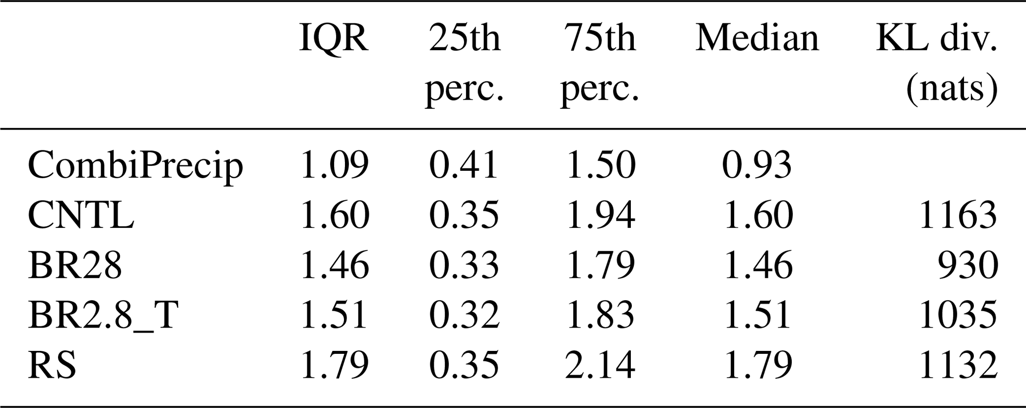
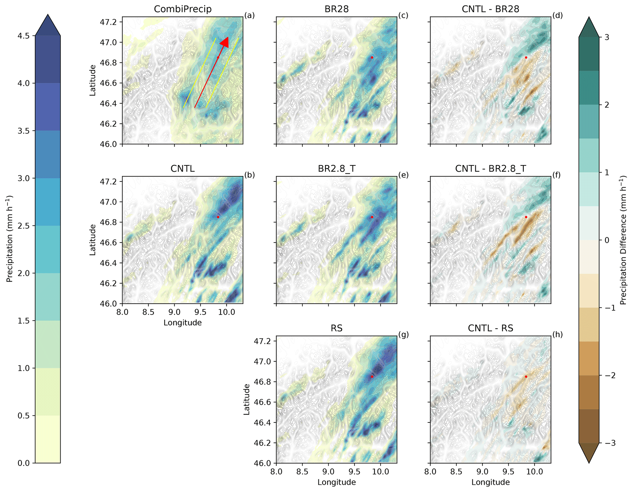
Figure 7 Precipitation rate (millimeters per hour; hereafter mm h⁻¹) over the domain. (a) CombiPrecip, (b) CNTL, (c) BR28, (d) CNTL − BR28, (f) CNTL − BR2.8_T and (h) CNTL − RS. between 12:00 and 14:00 UTC. The yellow lines are the outer limits of the cross sections around the red arrow showing the wind direction. The red marker shows the location of Gotschnagrat, and the gray shading is the topography between 0 (white) and 3700 m (dark gray).

In Fig. 7, we consider the precipitation over the larger domain (e.g., the red box in Fig. 1). The average wind direction between 12:00 and 14:00 UTC, and between 2 and 4 km above the surface, came from the southwest (indicated by the red arrow on Fig. 7a). To assess the skewed precipitation distribution between the CNTL and sensitivity simulations, the Kullback–Leibler divergence that measures the distances between asymmetric distributions was used. All the simulated precipitation distributions were more skewed towards the tail, overestimating the density between 2 and 4 mm h⁻¹ and underestimating the density between 1 and 2 mm h⁻¹ over the domain. The collisional breakup simulations diverge least from the observations, mainly due to the lower and more accurate densities at higher precipitation rates (Table 3 and Fig. 8). We calculated the interquartile ranges with the 25th and 75th percentiles to compare the precipitation distribution characteristics of the observations with the simulations. CombiPrecip had a narrower precipitation distribution, indicated by the interquartile range between the 25th and 75th percentiles of 1.09 mm h⁻¹, than all the simulations, meaning that the observed precipitation was less variable. This can be seen in the domain as all the simulations had regions of localized high precipitation rates. This resulted in a higher variability, with an interquartile range between 1.46 and 1.79 mm h⁻¹, of which 75 % of the precipitation was between 1.7 and 2.14 mm h⁻¹ (Fig. 8). The localized regions of stronger convection and invigorated precipitation when the SIP processes were excluded, causing the higher variability, can most likely initially be attributed to the dynamics. The microphysics scheme then further enhanced the precipitation overestimation in the localized regions. Craig and Dörnbrack (2008) demonstrated that a model resolution of ∼1 km is approximately equal to the characteristic turbulence scales of convective structures. Therefore, using a 1D turbulence scheme, which we used and is generally used in cloud-resolving models, is not optimal and in the “gray zone”. Also, horizontally homogeneous conditions are assumed in most turbulence schemes and have been validated over flat terrain (e.g., Mellor and Yamada, 1982; Rotach and Zardi, 2007), which is not the case for our study. As a result, the 1D turbulence scheme can underestimate the subgrid-scale variability in the vertical velocity. Earlier and higher precipitation rates can occur if the mountains are high enough to force the flow into an elevated mixed layer, leading to a faster transition of deep convection (Panosetti et al., 2018). From a microphysics point of view, the ice particles in the CNTL simulation are not multiplied through SIP and, therefore, can rapidly grow large, sediment out of the cloud at faster rates and overestimate the surface precipitation (Figs. 4e and 5e).

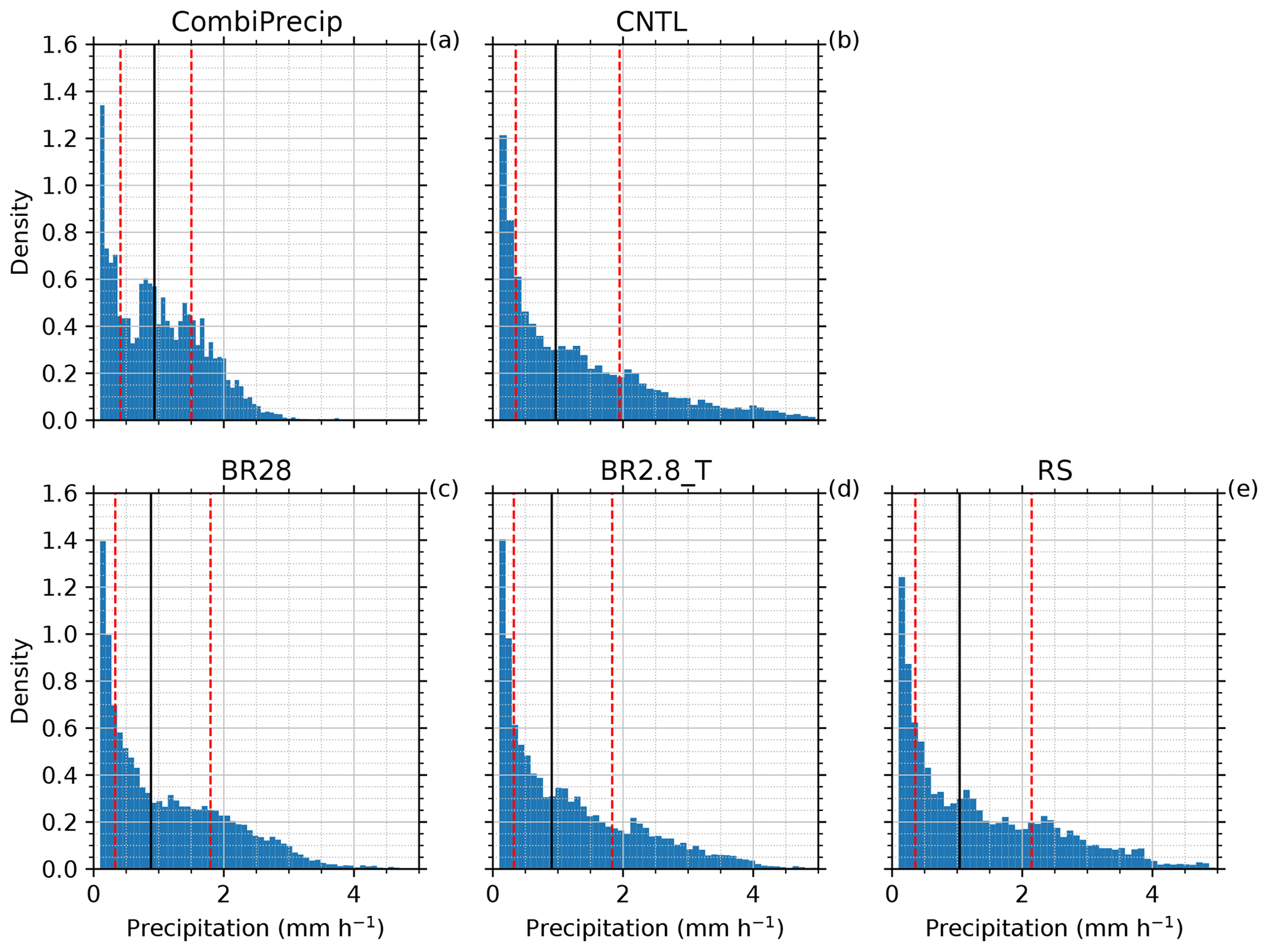
Figure 8 Precipitation rate (mm h⁻¹) histogram for (a) CombiPrecip, (b) CNTL, (c) BR28, (d) BR2.8_T and (e) RS from the domains in Fig. 7. The median (black solid line) and the 25th and 75th percentiles (red dashed line) are shown.

The localized regions of invigorated precipitation rates were suppressed by including the SIP processes (e.g., three cases are shown in Figs. S6 and S7). Because collisional breakup is a mechanical process, it does not contribute directly to the latent heat budget and, therefore, should not invigorate the updraft velocities. However, larger number concentrations of ice particles can cause increased depositional growth and, thereby, change the buoyancy structure of the cloud (Fig. S7). Stronger updrafts could then loft the smaller ice particles to higher altitudes, reducing their sedimentation velocities towards the surface. Evidence for the effect of the strong SIP rate on ice particle size can be seen in Figs. S4 and S5k–m. The BR28 simulation, which was able to produce the largest SIP rates, resembled the magnitude of the precipitation CombiPrecip the best by reducing more of the localized high precipitation regions of the CNTL simulation (e.g., Figs. 11 and S6). To the north of Gotschnagrat, the cloud was mostly glaciated, slowing precipitation down (Fig. 7c, f and i). Over the domain, the spread of the precipitation between the 25th and 75th percentiles was 1.46 mm h⁻¹, with 75 % of the precipitation below 1.79 mm h⁻¹ (Fig. 7c and d and Table 3). Another interesting feature is that the rime-splintering simulation caused a southward shift in the precipitation when compared to the CNTL simulation (Figs. 7b and h and 10g).

3.3 SIP impact on precipitation over the flow-oriented cross section

The flow-oriented vertical cross section, as depicted in Fig. 7, helps to explain the behavior of the MPC with respect to enhanced SIP (Fig. 9). The width of the cross section is ∼25 km, covering a majority of the precipitation along the cross section, as seen in the observations. It was chosen along the average wind direction during the analysis period, making it wide enough for robust results and, at the same time, not too wide so that the results become diluted. The MPC was defined by cloud droplet and ice mixing ratios greater than 10 and 0.1 mg m⁻³, respectively. In the CNTL and rime-splintering simulations, the mixed-phase part of the cloud extended to approximately 5 to 6 km and had a cloud top at 234 to 235 K. The rime-splintering rate below 4 km was confined to 0.1 L⁻¹s⁻¹, with the highest primary ice production rate of 0.01 to 0.1 L⁻¹s⁻¹ between 4 and 7 km. The structure of the MPC did not change significantly due to the enhanced SIP from rime splintering. The additional ice formation near the surface in the vicinity of the abundant cloud liquid water caused a significant increase in the averaged depositional growth rates over the cross section from 1.72 to 2.20 g m⁻² (an increase by 28 %), while the riming rates also showed a small increase (Figs. 9d and 10e and f). Higher mass mixing ratios in snow and graupel, also reflected in the higher ice water fraction, were produced as a result of the faster conversion from ice (Fig. 10a and c). This led to earlier and increased surface precipitation upstream of the flow direction over that of the CNTL simulation (Fig. 10g).

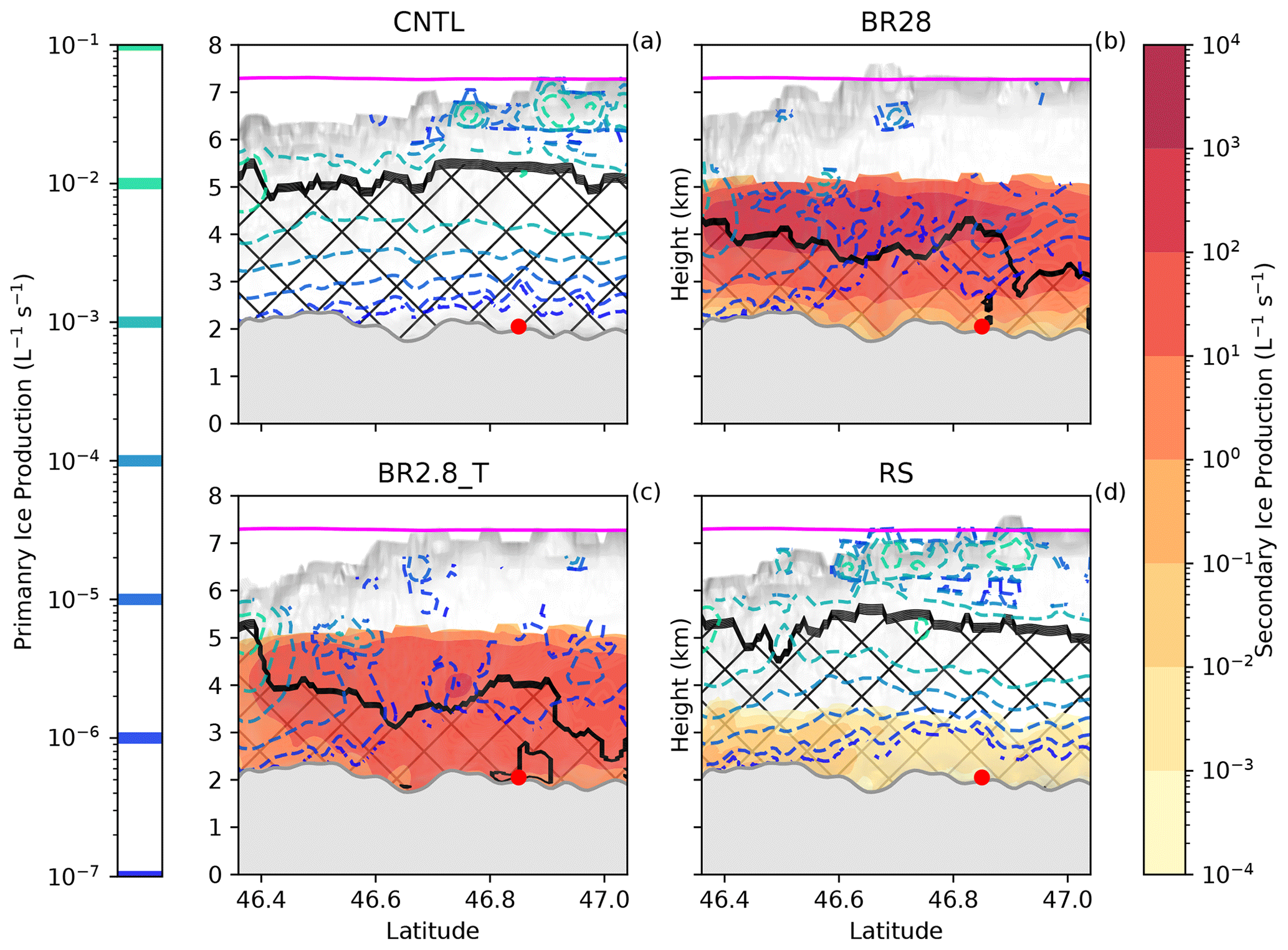
Figure 9 Primary ice production and secondary ice production (per liter per second; hereafter L⁻¹ s⁻¹) averaged between 12:00 and 14:00 UTC for (a) CNTL, (b) BR28, (c) BR2.8_T and (d) RS. The hatched area is defined as the MPC where the cloud droplet mass concentration and ice mass concentration is greater than 10 and 0.1 mg m⁻³, respectively. The pink line is the homogeneous freezing line at 235 K, and the shaded gray area is the cloud area fraction.

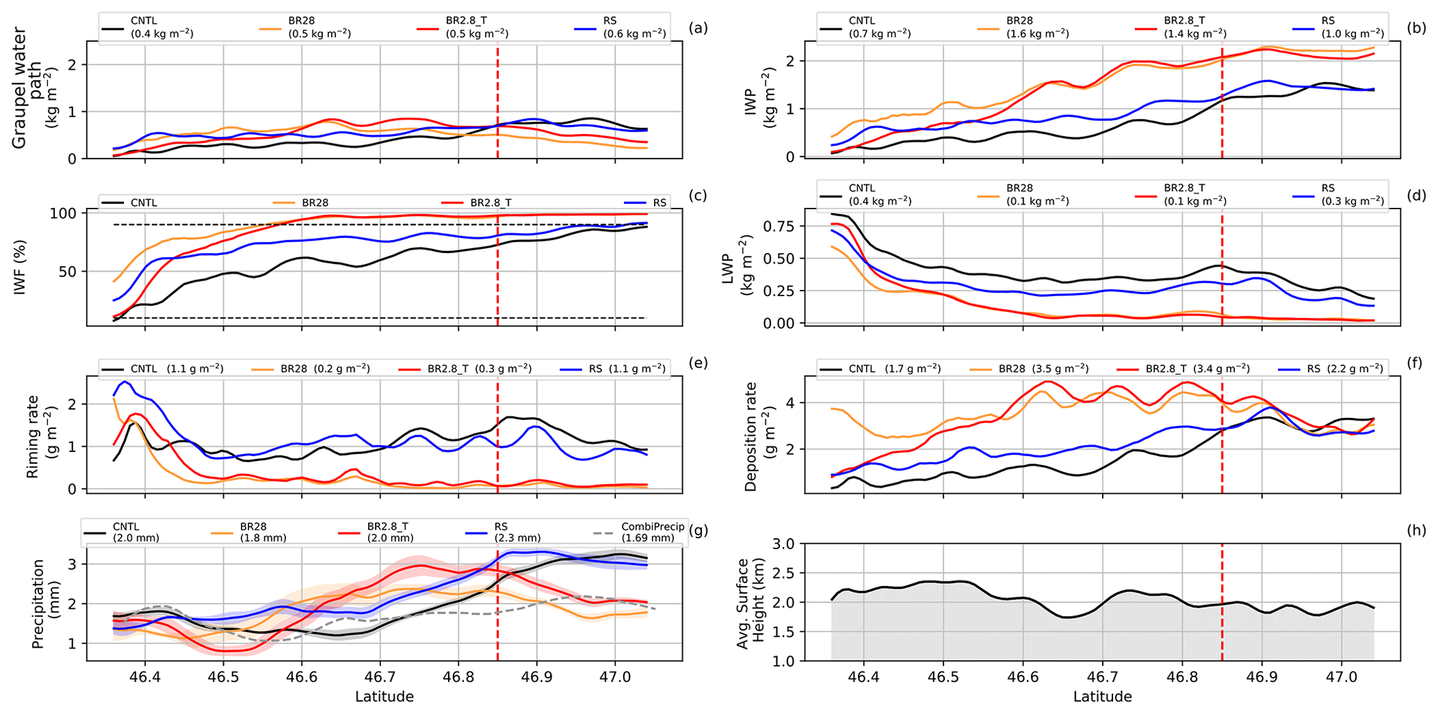
Figure 10 (a) Graupel water path, (b) IWP (ice water path), (c) IWF (ice water fraction) (IWP/(IWP + LWP)) × 100, (d) LWP, (e) riming rate and (f) deposition rate over the cross section. These quantities calculated in panels (a)–(f) were only over cloudy regions, where the cloud area fraction is larger than 0. In parentheses are the average over the latitude. Panel (g) shows the precipitation mean (solid line), ensemble spread (shaded area) and CombiPrecip (dashed line), and panel (h) shows the averaged topography over the cross section. The red vertical dashed line indicates the latitude of Gotschnagrat.

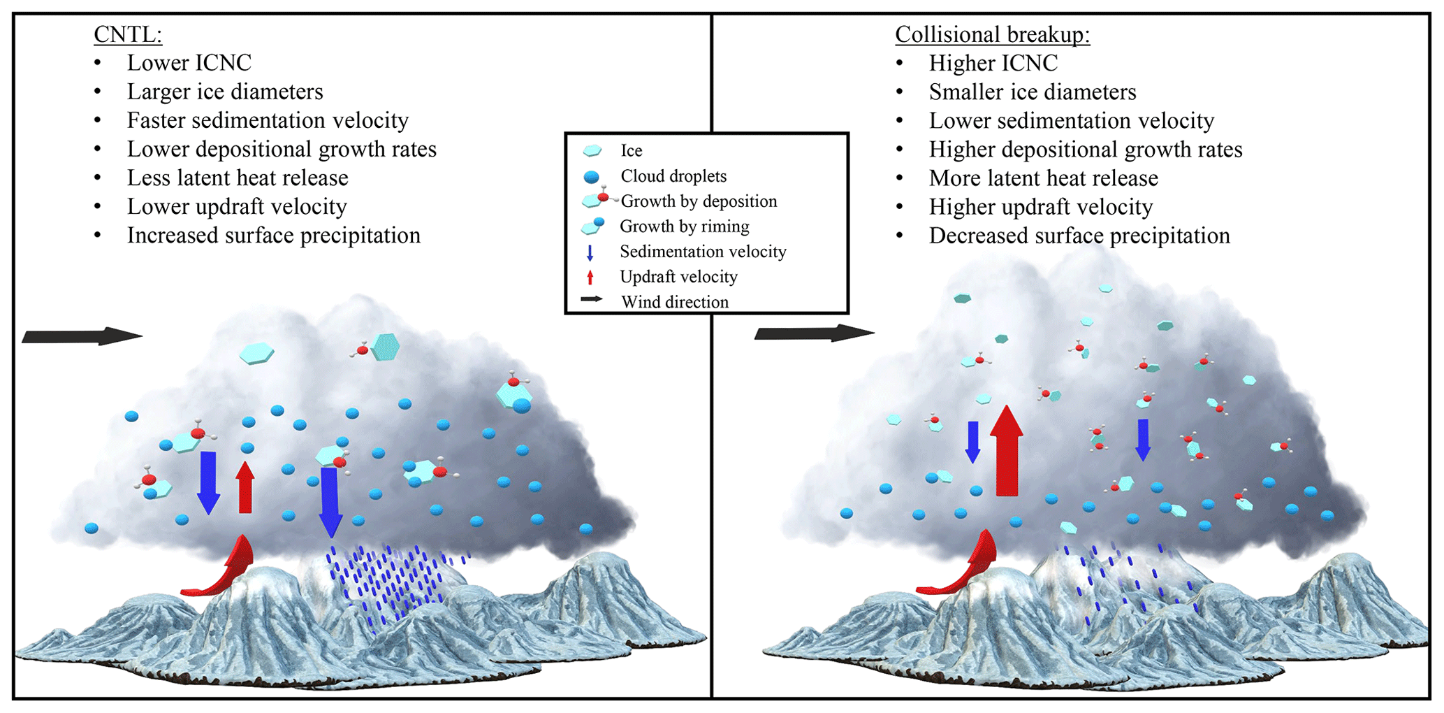
Figure 11 Schematic summary of the impact of collisional breakup of ice particles on the cloud structure and surface precipitation.

Collisional breakup had a distinct effect on the MPC, reducing its vertical extent to around 4 km (Fig. 9b and d). In both of the collisional breakup simulations, the SIP reached 100 L⁻¹ s⁻¹ below 5 km, impacting the primary ice production rate strongly due to the significant reduction in the LWP (Figs. 9b and 10d). As a result, there was a clear shift towards the depositional growth of ice particles from 46.4^∘ N northwards. Korolev and Mazin (2003) showed that, for high values of $N_i{\stackrel{\mathrm{‾}}{r}}_i$ and updraft velocities between 0.1 and 1 m s⁻¹, the ice particles will absorb water vapor rapidly, reducing it to saturation over ice and, therefore, controlling the supersaturation. Stronger combined growth rates of up to 33 % compared to the CNTL increased the latent heat release, updraft velocities and, ultimately, precipitation over the cross section between 46.5 and 46.8^∘ N. The BR2.8_T simulation, especially, overestimated the precipitation because of the higher SIP rates at warmer temperatures in the vicinity of cloud liquid water (Figs. 9c and 10g). North of 46.7^∘ N, the IWF was well above 95 %, glaciating large parts of the MPC. Because of the loss of cloud liquid, precipitation formation was slowed down, reducing the surface precipitation windward of Gotschnagrat (Fig. 10c to g). This resulted in a mean precipitation rate over the cross section that was 2 mm h⁻¹ compared to CombiPrecip at 1.69 mm h⁻¹. The BR2.8_T precipitation intensity lags behind that of the BR28 simulation over the flow-oriented vertical cross section (Fig. 10g). The faster precipitation formation is coupled to the higher ICNC within a MPC that can enhance riming, as long as liquid droplets are present, or else by the WBF process. The precipitation magnitude in the BR28 simulations matched the observed precipitation better but was shifted towards the south. In summary, we have provided evidence that COSMO may benefit from the inclusion of collisional breakup processes in simulating ICNC and precipitation.

4 Discussion

Our study suggests that including SIP through collisional breakup can enhance the in situ ICNC and, consequently, surface precipitation. The collisional breakup simulations led to ICNCs at Gotschnagrat of 1 to 2 orders magnitude larger than in the rime-splintering simulations. More precisely, the numbers were between 1 and 2 L⁻¹ and 10 and 12 L⁻¹ for BR28 and BR2.8_T, respectively, compared to the rime-splintering simulations of less than 0.1 L⁻¹. The BR28 simulation most closely reproduced observations, albeit leading to ICNC an order of magnitude smaller than observed at Gotschnagrat. However, blowing snow cannot be excluded as a contributor to the measured ICNC (e.g., Farrington et al., 2016; Beck et al., 2018; Walter et al., 2020) even though we were not able to quantify this process in our analysis. The resuspension of snow particles from the surface into the atmosphere where they could potentially interact with cloud particles is dependent on the wind speed. The total mass change of the snow pack is a function of the horizontal distribution of blowing snow, the sublimation rate of blowing snow, the sublimation/evaporation rates or condensation/deposition rate at the surface, the precipitation rate and the runoff of liquid water that all impact the mass change rate of a snowpack (Armstrong and Brun, 2008). Mahesh et al. (2003) have found that a threshold value for the wind speed above ∼7.6 m s⁻¹ is necessary to resuspend snow particles. More recently in the Swiss Alps, Walter et al. (2020) interpolated a threshold value of ∼7.5 m s⁻¹ from radar observations, which was in agreement with other studies (e.g., Li and Pomeroy, 1997). Wind speeds of larger than 7.5 to 15 m s⁻¹ could then transport these snow particles over distances of 60 to 240 m. In our case, the wind speeds recorded by the snowdrift station used by Walter et al. (e.g., 2020) were mostly below the 7.5 m s⁻¹ for the largest part of our analysis period (Fig. S8). However, between 12:45 and 13:30 UTC when wind speeds exceeded 7.5 m s⁻¹, a case can be made for blowing snow affecting the ice particle number concentration in the MPC and, thereby, triggering secondary ice processes. As a consequence, the current discrepancy in ICNC between the collisional breakup simulations and the observations could be overestimated.

Surprisingly, our SIP rate through collisional breakup was between 10⁴ and 10⁶ times larger than what Sullivan et al. (2018a) reported in their cold front rainband study. We hypothesize that this large difference is due to the availability of cloud liquid water that rimes onto ice and snow. This process converts ice and, especially, snow quickly to large quantities of graupel, which causes higher SIP rates through collisional breakup. In the Sullivan et al. (2018a) case, graupel was noticeably low, which limited graupel–ice/snow interactions. The low graupel concentrations meant that the SIP from collisional breakup simulation was at least 10³ times smaller than that of the rime-splintering simulation, which was at around 10 to 100 L⁻¹. The excessive SIP rate through collisional breakup in our simulations, in combination with a larger graupel mixing ratio (Fig. 10a), is likely due to ideal conditions for collisional breakup (Fig. 9 Sullivan et al., 2018b). Indeed, our simulations have a cloud base temperature of around 273 K and averaged updraft velocities through our cross section of up to 0.6 m s⁻¹. The large SIP rates, in our case, counteracted the stronger precipitation in localized regions. This decreased precipitation is in direct contrast to Sullivan et al. (2018a), showing that, when using SIP parameterizations, regions of invigorated precipitation became even wetter. The most likely explanation for the decrease in precipitation is that the smaller ice particles in our collisional breakup simulations that sediment slower reside longer in the cloud. Longer residence times increase the ability of ice particles to grow by vapor deposition and riming, thereby enhancing the latent heat release and, consequently, the updraft velocity. The higher updraft speed, in turn, can loft the ice particles to higher altitudes in the glaciated part of the cloud and, ultimately, alter the intensity and location of the surface precipitation (Fig. 11). If the middle to the upper part of the cloud were not glaciated, we would have indeed, similar to Sullivan et al. (2018a), expected a localized increase in surface precipitation due to faster ice particle growth (enhanced riming or enhanced WBF process). The SIP rates in our simulations compared better with Phillips et al. (2017a), even though they simulated a convective storm with updrafts exceeding 5 m s⁻¹, which is not comparable to the meteorological situation we simulated. However, in their case, the collisional breakup parameterization was more physically robust by including the kinetic energy of two particles, the fragility coefficients and humidity- and temperature-dependent collision types.

As stated in Sect. 2.2.3, we set an ICNC threshold of 2000 L⁻¹ in our model. This threshold strongly restricts the ICNC. Therefore, the full effect of using higher coefficients for F_BR could not be realized. We ran simulations with no ICNC threshold, resulting in a huge ICNC through which we observed evidence for artificially enhanced microphysics rates. For instance, the mean ice mass concentration is divided by the huge ICNC, resulting in a mean ice mass < $\mathrm{1}\times {\mathrm{10}}^{-\mathrm{12}}$ kg. Then, in the next model time step, the mean ice mass is increased to $\mathrm{1}\times {\mathrm{10}}^{-\mathrm{12}}$ kg (the minimum ice mass in COSMO), meaning that the calculated mean ice diameter is larger than at the previous time step. This can result in artificially increased deposition, riming and collision rates. This ICNC threshold is necessary, particularly in the collisional breakup simulations.

Another aspect that could enhance collisional breakup is the conversion from snow to graupel. For collisional breakup to occur, graupel formation is necessary. Graupel formation can only happen when either cloud droplets or raindrops rime onto ice or snow. Because snow in the model is described as pristine (unrimed), a tuning parameter is used to rapidly convert snow to graupel when raindrops rime onto snow (Seifert and Beheng, 2006). Alongside this tuning parameter, Seifert and Beheng (2006) set a threshold to convert ice and snow to graupel, only if they are larger than 500 µm in diameter, to suppress the early formation of very small, 200 to 400  µm, graupel. As soon as graupel forms within the collisional breakup regime (temperatures warmer than 252 K), the collisional breakup occurs. In the standard model version, the threshold has been set to 200 µm (e.g., Seifert and Beheng (2006)) which encourages earlier graupel formation. Using this threshold in conjunction with collisional breakup could be a reason why we simulated such large SIP rates. The representation of graupel also has other limitations. For instance, graupel has a fixed density and fall speed parameters, which is a less desirable representation of graupel that could substantially impact the collisional tendencies between graupel and other ice particles and affect SIP rates. It is worth considering the snow–graupel size conversion threshold and the graupel fall speed in further sensitivity studies when SIP processes are used in two-moment bulk microphysics schemes. Another limitation of bulk microphysics schemes is that the variability in observed drop size distributions in different regions within the same cloud or between different clouds is approximated by a gamma distribution with constant shape parameters (Costa et al., 2000; Geoffroy et al., 2010; Khain et al., 2015, and references therein).

A further consideration is to switch to a property-based microphysics scheme which focuses on the continuous evolution of the physical properties (e.g., density) of the ice particles (e.g., Morrison and Milbrandt, 2015; Milbrandt and Morrison, 2016; Jensen et al., 2017; Phillips et al., 2017b; Sotiropoulou et al., 2020) and which can support a more realistic representation of the collision breakup in orographic MPCs. A property-based scheme would also eliminate the limitation of two-moment bulk microphysics category-based hydrometeors. In the case of studying collisional breakup in summertime MPCs, the use of a three-moment bulk microphysics scheme can be beneficial, albeit much more computationally expensive, for simulating large hail (Milbrandt and Yau, 2006; Milbrandt and McTaggart-Cowan, 2010; Loftus and Cotton, 2014). These researchers showed that accurately reproducing the tail of a hail particle size distribution, which two-moment bulk microphysics schemes cannot replicate, is required for simulating large hail.

A popular assumption exists that bulk microphysics schemes (e.g., the Seifert and Beheng, 2006, scheme used in this work) are inherently less accurate than spectral bin microphysics schemes, which is not always the case. The main advantage of bulk microphysics schemes is their computational efficiency, being a factor of ∼30 computationally less expensive, making them much more appealing than spectral bin microphysics schemes. When ice-phase microphysics is considered, Seifert et al. (2006) showed the strength of the spectral bin scheme in simulating a squall line. Still, when the nucleation treatment of the spectral bin scheme was diagnosed with a bulk cloud condensation nuclei scheme, similar results were obtained in the accumulated precipitation to that of the bulk microphysics scheme. In addition, Xue et al. (2017) showed that spectral bin schemes, designed to be conceptually more realistic and therefore more accurate than bulk microphysics schemes, are quantitatively similar to the spread of bulk microphysics schemes when simulating the microphysical, thermodynamic and dynamic characteristics of a squall line. Khain et al. (2015) came to a similar conclusion. Therefore, it is within reason to expect that it is sufficient to study SIP with a two-moment bulk microphysics scheme.

5 Conclusions

Simulations of a cold front passage on 7 March 2019, during the RACLETS campaign in February and March 2019, were carried out with a non-hydrostatic, limited area atmospheric model, COSMO, that uses a two-moment cloud microphysics scheme with six hydrometeor categories. Additionally, two parameterizations, namely droplet shattering upon freezing and collisional breakup that occurs through ice-graupel collisions, were added to the already existing Hallett–Mossop parameterization (e.g., Sullivan et al., 2018a; Sotiropoulou et al., 2020). The simplified temperature-dependent collisional breakup parameterization is based on the work of Takahashi et al. (1995) and used here with different configurations of F_BR and γ_BR to account for the hydrometeor size scaling.

To conclude, our main findings can be summarized as follows:

• Droplet shattering did not show significant differences to the CNTL simulation. This is mainly due to the low raindrop number concentration present during the cold front passage over Gotschnagrat. Aside from using a shattering probability of 10 %, which is similar to Sullivan et al. (2018a), freezing raindrops in COSMO are spectrally partitioned into ice, snow and graupel, and only the partitioned ice is subject to shatter, which lowers the likelihood that this SIP proceeds (Blahak, 2008).

• Both the CNTL and rime-splintering simulations were not able to capture the ICNC observations at Gotschnagrat. The ice that formed via the primary ice processes above 3 km was mostly converted to snow and graupel, reducing the ICNC at the surface. Secondarily formed ice through rime splintering was, at most, 0.9 L⁻¹ at 3 km and decreased significantly below 3 km. The fact that small concentrations, of less than 0.5 mg m⁻³, of raindrops between 100 and 150  µm were available in the rime-splintering region and that Gotschnagrat was not in the rime-splintering temperature regime on 7 March limited the rime-splintering process. At Davos Wolfgang, none of the simulations could adequately represent the radar precipitation.

• The BR28 and BR2.8_T simulations showed enhanced ICNC at the surface compared to the CNTL simulations and reproduced the observed ICNC at Gotschnagrat very well. The enhanced SIP production did impact the cloud liquid water, reducing the LWP through the cloud layer and underestimating the LWP between 11:30 and 13:30 UTC at Davos Wolfgang. A 700 m shallow layer of cloud liquid water near the surface was maintained, causing cloud droplets and raindrops to rime onto the ice, corresponding to rime fractions of less than 5.4 %. However, this could not explain the HoloGondel observations showing that over 50 % of the ice crystals were rimed.

• During winter, when the thermal heating is minimal, the orography plays a significant role in lifting air parcels to higher altitudes, enhancing large drop formation and primary ice nucleation. These conditions are favorable for graupel formation and can result in enhanced collisional breakup. Therefore, collisional breakup may be more important in regions of strong orography than without during winter.

• The evidence suggests that including collisional breakup may be beneficial for simulating precipitation for this case study. The simulations presenting the stronger SIP, i.e., BR28, showed the most improvement in the timing and amount of surface precipitation during 7 March 2019. Regions of invigorated precipitations in the CNTL and rime-splintering simulations generally were more suppressed when the SIP parameterizations were used, bringing the simulated precipitations rates closer to the observations.