the Creative Commons Attribution 4.0 License.
the Creative Commons Attribution 4.0 License.
 | 11 Oct 2021
Time-dependent source apportionment of submicron organic aerosol for a rural site in an alpine valley using a rolling positive matrix factorisation (PMF) window
Gang Chen
Yulia Sosedova
Francesco Canonaco
Roman Fröhlich
Anna Tobler
Athanasia Vlachou
Kaspar R. Daellenbach
Carlo Bozzetti
Christoph Hueglin
Peter Graf
Urs Baltensperger
Jay G. Slowik
Imad El Haddad
André S. H. Prévôt
We collected 1 year of aerosol chemical speciation monitor (ACSM) data in Magadino, a village located in the south of the Swiss Alpine region, one of Switzerland's most polluted areas. We analysed the mass spectra of organic aerosol (OA) by positive matrix factorisation (PMF) using Source Finder Professional (SoFi Pro) to retrieve the origins of OA. Therein, we deployed a rolling algorithm, which is closer to the measurement, to account for the temporal changes in the source profiles. As the first-ever application of rolling PMF with multilinear engine (ME-2) analysis on a yearlong dataset that was collected from a rural site, we resolved two primary OA factors (traffic-related hydrocarbon-like OA (HOA) and biomass burning OA (BBOA)), one mass-to-charge ratio () 58-related OA (58-OA) factor, a less oxidised oxygenated OA (LO-OOA) factor, and a more oxidised oxygenated OA (MO-OOA) factor. HOA showed stable contributions to the total OA through the whole year ranging from 8.1 % to 10.1 %, while the contribution of BBOA showed an apparent seasonal variation with a range of 8.3 %–27.4 % (highest during winter, lowest during summer) and a yearly average of 17.1 %. OOA (sum of LO-OOA and MO-OOA) contributed 71.6 % of the OA mass, varying from 62.5 % (in winter) to 78 % (in spring and summer). The 58-OA factor mainly contained nitrogen-related variables which appeared to be pronounced only after the filament switched. However, since the contribution of this factor was insignificant (2.1 %), we did not attempt to interpolate its potential source in this work. The uncertainties (σ) for the modelled OA factors (i.e. rotational uncertainty and statistical variability in the sources) varied from ±4 % (58-OA) to a maximum of ±40 % (LO-OOA). Considering that BBOA and LO-OOA (showing influences of biomass burning in winter) had significant contributions to the total OA mass, we suggest reducing and controlling biomass-burning-related residential heating as a mitigation strategy for better air quality and lower PM levels in this region or similar locations. In Appendix A, we conduct a head-to-head comparison between the conventional seasonal PMF analysis and the rolling mechanism. We find similar or slightly improved results in terms of mass concentrations, correlations with external tracers, and factor profiles of the constrained POA factors. The rolling results show smaller scaled residuals and enhanced correlations between OOA factors and corresponding inorganic salts compared to those of the seasonal solutions, which was most likely because the rolling PMF analysis can capture the temporal variations in the oxidation processes for OOA components. Specifically, the time-dependent factor profiles of MO-OOA and LO-OOA can well explain the temporal viabilities of two main ions for OOA factors, 44 (CO) and 43 (mostly C2H3O+). Therefore, this rolling PMF analysis provides a more realistic source apportionment (SA) solution with time-dependent OA sources. The rolling results also show good agreement with offline Aerodyne aerosol mass spectrometer (AMS) SA results from filter samples, except for in winter. The latter discrepancy is likely because the online measurement can capture the fast oxidation processes of biomass burning sources, in contrast to the 24 h filter samples. This study demonstrates the strengths of the rolling mechanism, provides a comprehensive criterion list for ACSM users to obtain reproducible SA results, and is a role model for similar analyses of such worldwide available data.
- Article
(9730 KB) - Full-text XML
-
Supplement
(10839 KB) - BibTeX
- EndNote


Atmospheric particulate matter (PM) affects human health and climate. In particular, it influences the radiative balance (IPCC, 2014; von Schneidemesser et al., 2015), reduces visibility (Chow et al., 2002; Horvath, 1993), and negatively affects human health by triggering respiratory and cardiovascular diseases and allergies (Daellenbach et al., 2020; Dockery and Pope, 1994; Mauderly and Chow, 2008; Monn, 2001; Pope and Dockery, 2006; von Schneidemesser et al., 2015). Fine PM exposure strongly correlates with the global mortality rate. Lelieveld et al. (2015) estimated that outdoor air pollution, mostly PM2.5 (PM with an aerodynamic diameter smaller than 2.5 µm), causes 3.3 million premature deaths per year worldwide. Despite this correlation, different aerosol sources may have strongly different effects on health (Daellenbach et al., 2020). Thus, both climate and health effects are affected by particle chemical composition, which is related to emission sources of primary particles and precursor gases for secondary aerosol (IPCC, 2014; Jacobson et al., 2000; Jacobson, 2001; Lelieveld et al., 2015; Ramanathan et al., 2005).
Organic aerosol (OA) constitutes 20 %–90 % of fine PM (Jimenez et al., 2009; Murphy et al., 2006; Zhang et al., 2007) and contain millions of chemical compounds. Since OA is the subject of an extremely complex mixture of chemical constituents, with highly dynamic spatial and temporal (seasonal, diurnal, etc.) variability in directly emitted particles and gas-phase precursors and complex chemical processing in the atmosphere, elucidation of the chemical composition and physical properties of OA remains challenging. Identification and quantification of OA sources with a sophisticated interpolation of spatial and temporal variabilities are essential for developing effective mitigation strategies for air pollution and a better assessment of the aerosol effect on both health and climate.
OA source apportionment (SA) and PM composition have been studied extensively using an Aerodyne aerosol mass spectrometer (AMS) (Canagaratna et al., 2007). However, due to the complexity of the AMS measurements and their high operational expenses, AMS campaigns are often limited to short periods of a few weeks to months. The aerosol chemical speciation monitor (ACSM) allows for unattended long-term observation (> 1 year) of non-refractory aerosol particles (Ng et al., 2011a; Fröhlich et al., 2013). It also makes it possible to investigate the long-term temporal variations in OA sources, which is crucial for policymakers to introduce or validate aerosol-related environmental policies.
Positive matrix factorisation (PMF; see Sect. S3.1 in the Supplement) has been used in various studies for SA of OA (Lanz et al., 2007; Aiken et al., 2009; Hildebrandt et al., 2011; Zhang et al., 2011; Mohr et al., 2012; Schurman et al., 2015). The multilinear engine (ME-2) implementation of PMF (Paatero, 1999) improves model performance by allowing the use of a priori information (constraints on source profiles and/or time series) to direct the model towards environmentally meaningful solutions (Canonaco et al., 2013; Crippa et al., 2014; Fröhlich et al., 2015; Lanz et al., 2008; Ripoll et al., 2015). For long-term data (1 year or more) with a high time resolution, the composition of a given source could change considerably due to meteorological and seasonal variabilities. However, a major limitation of PMF is the assumption of static factor profiles, such that it fails to respond to these temporal changes. Therefore, long-term chemically speciated data have been evaluated monthly or seasonally (Petit et al., 2014; Canonaco et al., 2015; Minguillón et al., 2015; Ripoll et al., 2015; Bressi et al., 2016; Reyes-Villegas et al., 2016) to take at least the seasonal variations into account. To improve the analysis of long-term ACSM datasets, a novel approach that utilises PMF analysis over a shorter rolling time window was first proposed by Parworth et al. (2015) and further refined using ME-2 by Canonaco et al. (2021). The short length of the rolling PMF window allows the PMF model to take the temporal variations in the source profiles into account (e.g. biogenic versus domestic burning influences on oxygenated organic aerosol (OOA)), which normally provides better separation between OA factors. In addition, using this technique together with bootstrap resampling and a random a-value approach allows users to assess the statistical and rotational uncertainties in the PMF results (Canonaco et al., 2021; Tobler et al., 2020).
In this work, we conducted a 1-year ACSM measurement campaign from September 2013 to October 2014 in Magadino, located in an alpine valley in southern Switzerland. We present a comprehensive analysis of the ACSM dataset measured in Magadino using a novel PMF technique, the “rolling PMF”. In addition, we also compare the results of the rolling PMF with the SA of offline AMS filter samples (Vlachou et al., 2018) and conventional seasonal PMF analysis.
2.1 Sampling site
Magadino, where the sampling site is located, is in a Swiss alpine valley ( N, E; 204 m a.s.l.). This site belongs to the Swiss National Air Pollution Monitoring Network (NABEL, https://www.empa.ch/web/s503/nabel, last access: 20 July 2021). It is around 1.4 km away from the local train station, Cadenazzo; around 7 km away from Locarno Airport; and nearly 8 km away from Lake Maggiore. This station is surrounded by agricultural fields within a rural area and is considered a rural background site. It can be potentially affected by domestic wood burning, adjacent agricultural activity, and transit traffic through the valley. The site topography favours quite high PM levels due to stagnant meteorological conditions or boundary layer inversions, especially in winter. Magadino remains one of the most polluted regions in Switzerland, and it has often exceeded the annual average PM10 limit value for Switzerland (20 µg m−3) (Meteotest, 2017; The Swiss Federal Council, 2018). Therefore, there is an increasing need for a more effective mitigation strategy.
2.2 ACSM measurements
This study measured chemical composition and mass loadings of non-refractory constituents of ambient submicron aerosol particles (NR-PM1) by an Aerodyne quadrupole ACSM (Ng et al., 2011a). The ACSM uses the same sampling and detection technology as the AMS but is simplified and designated for long-term monitoring applications by reducing maintenance frequency at the cost of lower sensitivity, restriction to the integer mass resolution, and no size measurement. As for the AMS, sampled submicron particles enter the instrument through a critical orifice (100 µm i.d.) at a flow rate of 1.4 cm3 s−1 (at 20 ∘C and 1 atm). The sampling flow will pass either through a particle filter or directly into the system using an automated three-way switching valve that is switched every ∼ 30 s. An aerodynamic lens focuses the sampled particles into a narrow beam which impacts on a tungsten surface of around 600 ∘C, where the non-refractory particles vaporise and are subsequently ionised by an electron impact source (70 eV). A quadrupole mass spectrometer detects the resulting ions up to a mass-to-charge ratio () of 148 Th. The particle mass spectrum is represented by the difference between the total ambient air and particle-free signals.
The quantification of ACSM data requires an estimation of the fraction of NR-PM1 that bounces off the oven without being vaporised and therefore is not detected (Canagaratna et al., 2007; Matthew et al., 2008). In this study, a constant collection efficiency (CE) factor of 0.45 was applied to take it into account. The details of determinations of the CE value is described in Sect. S1 in the Supplement. In this study, we recorded the data with a time resolution of 30 min. During the campaign, the ACSM filament burnt out on 14 April 2014. This was addressed by switching to the backup filament installed within the instrument (no venting required). Calibration of the relative ionisation efficiencies (RIEs) of particulate nitrate, sulfate, and ammonium was conducted using size-selected (300 nm) pure NH4NO3 and pure (NH4)2SO4 particles. Calibrations of the RIE, scale, and the sampling flow were performed every 2 months. In this study, we used the averaged RIEs for nitrate, sulfate, and ammonium. The exact values are shown in Fig. S1 of the Supplement.
2.3 Complementary measurements
Meteorological data, including temperature, precipitation, wind speed, wind direction, and solar radiation, are monitored at the NABEL station. In addition, concentrations of trace gases (SO2, O3, NOx), equivalent black carbon (eBC), and PM10 were measured with a time resolution of 10 min. We used an aethalometer (AE31 model by Magee Scientific) to measure eBC concentrations. Therefore, we conducted SA of eBC by following Zotter et al. (2017) using Ångström exponents for eBC from traffic αtr=0.9 and wood burning αwb=1.68. More details about eBC source apportionment are provided in Sect. S2 of the Supplement.
2.4 Preparation of the data and error matrices for PMF
In this study, we used acsm_local_1610 software (Aerodyne Research Inc.) to prepare the PMF input matrix. In total, this dataset includes 19 708 time points and 67 ions. Of these, CO-related variables ( ( 16), ( 17), and ( 18)) were excluded from the spectral matrix prior to a PMF analysis. They are reinserted into the OA factor mass spectra after the PMF analysis using the ratio from the fragmentation table (Allan et al., 2004); the factor concentrations are likewise adjusted. According to Allan et al. (2003, 2004), the measurement error matrix was calculated with a minimum error considered for the uncertainty in all variables in the data matrix as in Ulbrich et al. (2009). Following the recommendations in Paatero and Hopke (2003) and Ulbrich et al. (2009), the measurement uncertainty for variables () with a signal-to-noise ratio (S N) < 2 (weak variables) and S N < 0.2 (bad variables) was increased by a factor of 2 and 10, respectively. In total, 27 weak ACSM variables were down-weighted. Additionally, 12 and 13 were not considered during the PMF analyses due to being noisy and their overall negative signal. Moreover, 15 was not only very noisy (S N = 0.09) but maybe also affected by high biases due to potential interference with air signals.
2.5 Rolling PMF analysis with ME-2
In this study, we conducted a series of steps (Sect. S3.2 and S3.3 in the Supplement) to obtain the results we present in this paper. In summary, we first tested potential sources for each season with seasonal PMF pre-tests. Secondly, we obtained stable seasonal solutions from bootstrap seasonal analysis. Then, we conducted rolling PMF with certain settings (constraints, number of repeats, length of the window size, and step of rolling window). Lastly, we were able to retrieve robust results using specific criteria to define environmentally reasonable solutions. Please refer to Sect. S3.2 and S3.3 in the Supplement for more detailed description of each step. This section focuses on the general introduction of rolling PMF with ME-2, the differences between our method vs. the method developed by Canonaco et al. (2021), and the general settings of the rolling PMF analysis in this study.
Running PMF over the long-term ACSM datasets assumes that the OA source profiles are static within this time window. It can lead to large errors since OA chemical fingerprints are expected to vary over time (Paatero et al., 2014). For example, Canonaco et al. (2015) showed that summer and winter OOA variability cannot be accurately represented by a single pair of OOA profiles. A common way to reduce the model uncertainty arising from this source is to choose a proper number of OA factors (Sug Park et al., 2000) and then perform a PMF analysis on a subset of measurements to capture temporal features of OA chemical fingerprints. Such characterisation of OA sources on a seasonal basis has been demonstrated in several studies (Lanz et al., 2008; Crippa et al., 2014; Petit et al., 2014; Minguillón et al., 2015; Ripoll et al., 2015; Zhang et al., 2019). Parworth et al. (2015) introduced the rolling PMF by running PMF in a small window (14 d), which advanced with a step of 1 d. This novel technique enables the source profiles to adapt to the temporal variabilities. Canonaco et al. (2021) combined the rolling PMF technique with ME-2 (Sect. S3.1 in the Supplement) to deal with the rotational ambiguity of the PMF analysis. In addition, it also used the bootstrap resampling strategy (Efron, 1979) and random a values (Sect. S3.2.2 in the Supplement) to estimate the statistical and rotational uncertainties in the PMF analysis.
This study mostly followed the methods developed by Canonaco et al. (2021) but with some modifications. The settings of the rolling PMF window is explicitly explained in Sect. S3.2.3 of the Supplement). In addition, we also performed a test of the rolling window size (i.e. 1, 7, 14, and 28 d) using a similar approach (Sect. S4 in the Supplement). As Canonaco et al. (2021) did, we also used the criteria-based selection function developed by Canonaco et al. (2021) to evaluate our PMF runs. The settings of the criteria are provided in Sect. S3.2.4 of the Supplement.
However, instead of using published reference factor profiles like Canonaco et al. (2021) have done, we retrieved the reference profiles of primary and local factors from seasonal bootstrap analysis (Sect. S3.2 in the Supplement). Specifically, the reference profiles of the hydrocarbon-like OA (HOA) factor and biomass burning OA (BBOA) factor were retrieved from the winter (December, January, and February; DJF) bootstrapped PMF solution as shown in Fig. S4, and we obtained the 58-related (58-OA) factor profile from the summer (June, July, and August; JJA) bootstrapped PMF solution (Fig. S4). The 58-OA factor was dominated by nitrogen-containing fragments (at 58, 84, and 98). In general, the ACSM estimates the organic 98 signal by dividing organic 84 by a factor of 2 according to the fragmentation table of organic species that was provided by Allan et al. (2004). Thus, the intensity of 98 is always half of the intensity of 84 in each factor. This 58-OA factor appeared only after the filament was switched on 14 April 2014. The instrument setup thus strongly influenced the sensitivity of these components due to influences of surface ionisation. The nitrogen-containing ion, 58, was also observed in Hildebrandt et al. (2011) due to the enhanced surface ionisation in a certain period. In addition, the potassium signal was enhanced at the same time, which further corroborated our hypothesis of the enhanced surface ionisation. Also, since this factor was constrained through the whole dataset, the PMF model overestimated the mass concentration of this factor significantly, which leads to high uncertainties for the 58-OA factor. Therefore, the time series of this source should be considered the upper limit, and the real mass concentration of it could be substantially lower. However, with the low mass concentration of the 58-OA factor during the whole campaign, we considered it a minor factor. Thus, this factor was considered in the PMF analysis, but no further interpretation of its potential source will be attempted in this paper. Moreover, we took a different path to define “good” PMF solutions by using a novel Student t-test approach to determine the environmentally reasonable solutions quantitatively with minimum subjective judgements (Sect. S3.3 in the Supplement). Overall, we provided a comprehensive analysis of a long-term ACSM dataset using this state-of-the-art technique in this work. The results are presented in the following section.
3.1 Overview of PM1 sources in Magadino
Considering that the major part of eBC is within PM1 (Schwarz et al., 2013), we added eBC to the total NR-PM1 from the ACSM to perform a mass closure analysis using independent measurements of PM2.5 and PM10 from filters. The gravimetric PM2.5 and PM10 show a high correlation with the total estimated PM1 (NR-PM1+eBC) (Fig. S1c). The slopes of the linear fits (±1 standard deviation) are 1.62 ± 0.05 (r2=0.81; N=79) for PM2.5 vs. PM1 and 1.84 ± 0.03 (r2=0.67; N=335) for PM10 vs. PM1. This means that the estimated PM1 comprised 62 % and 54 % of the PM2.5 and PM10 mass, respectively. The daily averages of inorganic species concentrations measured by the ACSM and those measured on the filters by ion chromatography showed a good correlation, with r2=0.83 for SO, r2=0.82 for NO and r2=0.50 for Cl−, with slopes close to 1 (Fig. S1a). The 2-week average of total ammonium and total nitrate measured by the offline AMS technique agreed rather well with the ACSM ammonium (47) and nitrate (r2=0.79), as shown in the plots in Fig. S1b. The ion balance of particulate ammonium, sulfate, and nitrate measured by the ACSM showed that the measured aerosol particles were mostly neutral.
The daily average PM1 components are shown in Fig. 1a, with an annual average PM1 concentration (including eBC) from September 2013 to October 2014 equal to 10.2 µg m−3. In winter, the average PM1 concentration was highest (13.8 µg m−3), with OA contributing 54 % to the total PM1 mass. In summer, the average PM1 mass concentration was below 10 µg m−3, but the relative contribution of the OA fraction increased to 62 %.
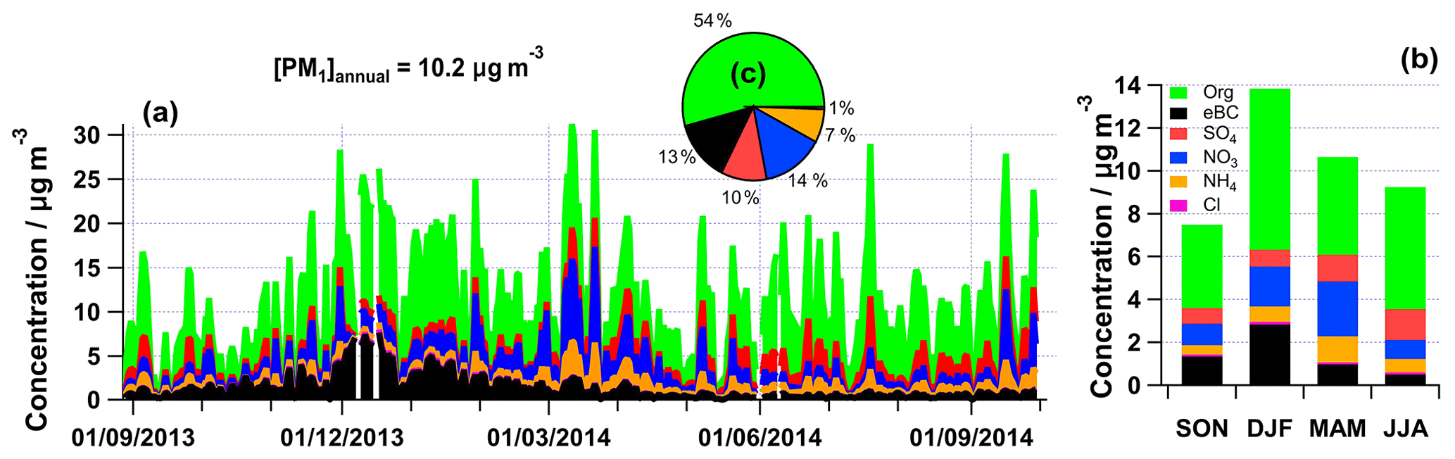
Figure 1Chemical composition of PM1 in Magadino 2013–2014 – daily (a), seasonal (b), and annual (c) averages. The labels indicate non-refractory organics (Org), sulfate (SO4), nitrate (NO3), ammonium (NH4), and chloride (Cl) measured by the ACSM and equivalent black carbon (eBC) measured by light absorption.
Seasonally averaged diurnal cycles of NR-PM1 components and eBC are displayed in Fig. 2. In this study, all the data are based on local time (central European time). In autumn, spring, and summer, the diurnals of these pollutants seem to be mainly affected by the development of the boundary layer height (BLH). Most of the species show similar diurnal trends for these three seasons. In addition, summer has the highest sulfate concentration due to enhanced photochemical production. In winter, air pollutants accumulate during the evening and night due to thermal inversion. In general, eBC and organics have higher levels due to enhanced biomass burning emissions and a lower BLH. We observed distinct midday peaks of organics, sulfate, nitrate, ammonium, chloride, and NOx in the winter. Magadino experienced a series of windless and cold but sunny periods from December 2013 to January 2014, including such sharp peaks (Fig. S6a). This was due to advection within the shallow boundary layer as both primary and secondary pollutants increased simultaneously. At the same time, the local wind speed near the ground was very low. One potential explanation was that the locally and regionally induced orography-influenced winds, including vertical diffusion processes, caused these delayed midday peaks. However, these processes remain difficult to track without spatially distributed measurements. Such phenomena were not observed during cloudy, cold, and windless days (Fig. S6b) without thermally induced meteorological processes. Unlike in other seasons, the dilution process due to vertical mixing happened only after noon due to strong inversions during the night and late irradiation of the valley surface in the winter.
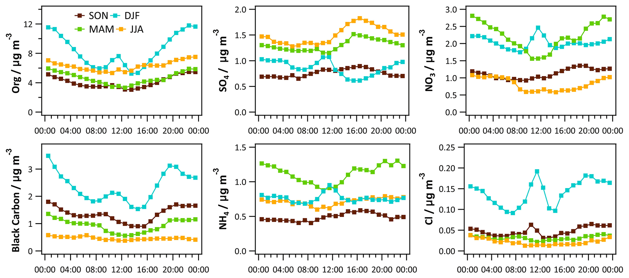
Figure 2Seasonal, diurnal cycles of the measured PM1 components (hourly averages) for the organic and inorganic species (sulfate, nitrate, ammonium, and chloride) of the ACSM and equivalent black carbon.
3.2 Seasonal PMF pre-tests
The automated rolling PMF analysis requires the knowledge of the reference profiles as well as the number of factors. This section presents how the number of factors was determined based on seasonal PMF pre-tests (refer to Sect. S3.2.1 in the Supplement for methodology). Initially, unconstrained PMF (three to six factors) was performed separately for the different seasons by following the SA guidelines provided by Crippa et al. (2014). Typically, the HOA profile is characterised by a high contribution of alkyl fragments (e.g. 43, 57) and the corresponding alkenyl carbocations (e.g. 41, 55), and the factor profile is relatively consistent over time and different locations. The BBOA profile exhibits significant signals at 60 and 73, which are well-known fragments arising from the fragmentation of anhydrous sugars present in biomass-related emissions (Alfarra et al., 2007). The HOA profile is present throughout the whole year for the unconstrained PMF runs, while the BBOA profile exists for all seasons except in summer. However, as shown in Fig. S2, the measured fraction of 60 during summer was above the background level of 0.3 % ± 0.06 % for biomass-burning-related air masses (Aiken et al., 2009; Cubison et al., 2011; DeCarlo et al., 2008). In addition, the scaled residual at 60 was decreased when a BBOA factor profile was constrained. Thus, we decided to constrain the BBOA factor for all seasons to potentially capture local events, such as open fires and barbecues in summer.
No evidence for the presence of a cooking-related OA (COA) factor was found based on the seasonal pre-analysis of the key fragments ( 55 and 57). Figure S3 shows no difference in the slope of the absolute mass concentration of 55 vs. 57 for different hours of the day (Fig. S3a), while different seasons show different slopes (Fig. S3b). Therefore, a COA factor was not considered in the PMF model. Moreover, a rapid increase in the measured fraction of 58, 84, and 98 together with 39 (potassium signal) was observed after a filament exchange on 14 April 2014. It was likely that the ACSM's sensitivity towards those ions was changed by the filament exchange. Also, this 58-OA factor was present for spring, summer, and autumn in 2014 in unconstrained PMF runs all the time after the filament change. Therefore, we kept this factor for these three seasons.
For the factor(s) with a secondary origin, we performed PMF models with a different number of factors (three–six) to assess if the oxygenated OA (OOA) factor is separable without mixing with primary organic aerosol (POA) factors (with a high contribution of 44 that is likely dominated by the CO ion, derived from decomposition of carboxylic acids; Duplissy et al., 2011). We conducted these tests (with a different number of factors) independently for the different seasons (autumn 2013, winter, spring, summer, autumn 2014).
We analysed the winter data first by constraining an HOA factor profile (Crippa et al., 2013) with a tight a value of 0.05. The three-factor solution (with one OOA factor, i.e. less oxidised OOA (LO-OOA) and more oxidised OOA (MO-OOA)) showed similarly good agreement of HOA and BBOA with the external tracers (NOx, eBC from traffic sources (eBCtr), eBC from wood burning sources (eBCwb)) to that of the four-factor solution (with two OOA factors). However, the scaled residual of 60 was reduced for the solution with two OOA factors. Moreover, the solution with one OOA factor was not sufficient to explain the variabilities in measured f44 vs. f43 (excluding the primary organic aerosol (POA) factors). For five- and six-factor solutions, the BBOA and LO-OOA factors started to split. Eventually, we selected the four-factor solution (HOA, BBOA, MO-OOA, LO-OOA) as the best representation of the winter data.
After the bootstrap seasonal PMF runs of the winter data (details in Sect. S3.2.2 of the Supplement), we extracted the HOA and BBOA profiles to use them as the reference factor profiles (Fig. S4) for the pre-tests of other seasons. For the spring, summer, and autumn seasons, three- to six-factor PMF solutions were modelled separately for each season by constraining the HOA (a value = 0.1) and BBOA (a value = 0.3) profiles. For the three-factor solution, we observed an OOA factor with some signals at 58, 84, and 98, which we could not relate to a specific source or process. Also, the scaled residuals of variables showed significant levels for these three ions. In addition, the time series and factor profile of 58-OA were so distinct that PMF could easily resolve it. When we increased the number of OA factors from three to four, a factor dominated by 58, 84, and 98 emerged, named the 58-OA factor. However, the OOA factor still showed slight signals at 58, 84, and 98. An increase in the number of factors from four to five resulted not only in a decrease in but also in “clean” OOA factors without mixing with the 58-OA factor. A further increase in the number of factors did not change substantially (< 1 %), and the sixth factor was a mathematical split of the 58-OA factor with 58 as the dominating variable. Thus, the five-factor PMF model was chosen as the most appropriate for the spring, summer, and autumn 2014 to isolate this instrumental artefact via PMF. We did not add the 58-OA factor for the autumn season in 2013 since it appeared only after the filament exchange on 14 April 2014. This 58-OA factor was included while running PMF because of the rapid drop of the from four to five factors in the PMF model, but the source of this factor will not be discussed in the paper.
3.3 Full-year rolling PMF analysis
Here we present the optimised time window size (14 d) (details of the time window optimisation are given in Sect. S4 of the Supplement and in Fig. S10). In total, we considered 53.4 % of the PMF runs (11 087 out of 20 750) with only 11 non-modelled data points. The results of the full-year PMF analysis of the 30 min resolved ACSM data are summarised in Fig. 3. The relative contributions of the OA factors are in addition shown in Fig. 3b. The primary traffic-related HOA had tiny variation (seasonal averages between 8.1 % and 10.1 %) throughout the year (Fig. 4). In contrast, BBOA showed a distinct yearly cycle (8.3 %–27.4 %) with a yearly averaged contribution of 17.1 %. They increased significantly (to 27.4 %) in winter which is typical of Alpine valleys (Szidat et al., 2007). This means that biomass burning was the most important primary OA source during the cold season in Magadino. The eBCwb showed similar trends to those of the BBOA factor time series during the cold seasons (Fig. 3c). The contribution of the 58-OA factor remained small before the filament was changed on 14 April 2014, which was expected because we could not retrieve this factor in seasonal, unconstrained PMF runs before April 2014.
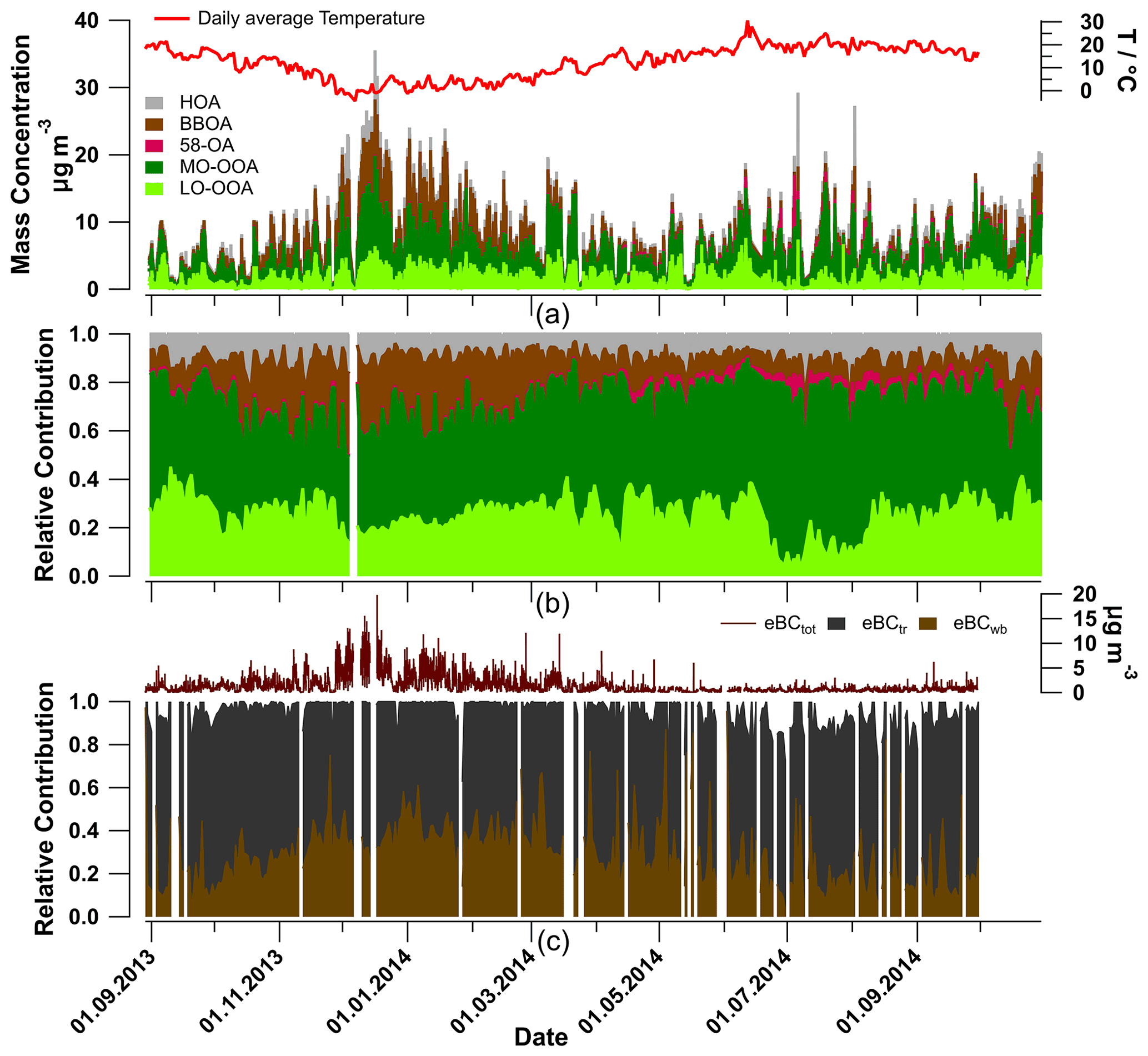
Figure 3Annual cycles of OA components: (a) absolute and (b) relative OA contributions plotted as 30 min resolved time series, and (c) black carbon source apportionment.
In this study, we retrieved two OOA factors, LO-OOA and MO-OOA. Total OOA (LO-OOA + MO-OOA) contributed substantially to the total OA mass throughout the whole year, with an average contribution of 71.6 % (Figs. 3b, 4). In general, the contribution of OOA to the total OA mass did not vary distinctly over the seasons but reached a maximum of 90.1 % on 12 June 2014, the day with the highest daily average temperature (30.7 ∘C).
In this work, we made head-to-head comparisons between the seasonal bootstrap solutions and the rolling PMF results (see Figs. A1–A3 and Table A1 in the Appendix) in terms of mass concentrations, factor profiles, scaled residuals, and correlations between time series for each factor and corresponding external tracers. We found consistent factor profiles and mass concentrations for the constrained factors (i.e. HOA, BBOA, and 58-OA), while OOA factors showed some noticeable differences in both mass concentrations and factor profiles. Rolling PMF provided slightly better correlations and smaller scaled residuals. Therefore, we consider rolling PMF results to be more environmentally reasonable than those of the seasonal PMF (more details in Appendix A).
3.3.1 Optimised OA factors retrieved from a rolling PMF model
The primary and secondary OA factors retrieved as an annual mean of all optimised PMF solutions together with their diurnal cycles for all seasons are shown in Fig. 5. Note that the primary factors (HOA, BBOA, and 58-OA) were constrained: the 58-OA profile was tightly constrained with an a value of 0.05 due to the uniqueness of its chemical profile, while the HOA and BBOA model profiles varied more due to looser constraints (Fig. S8). HOA and BBOA had averaged a values of 0.207 ± 0.036 and 0.195 ± 0.050, respectively. In addition, they both showed good agreement with previous studies (Crippa et al., 2014; Ng et al., 2011b). The probability distribution function (PDF) of applied a values for selected PMF runs vs. time was also investigated (Fig. S8). Most selected runs chose a values of 0.1–0.3 for HOA and BBOA. The OOA factors show more significant variations in the chemical profiles because these two factors were not constrained due to the high variability in oxidation processes governing the secondary factors.
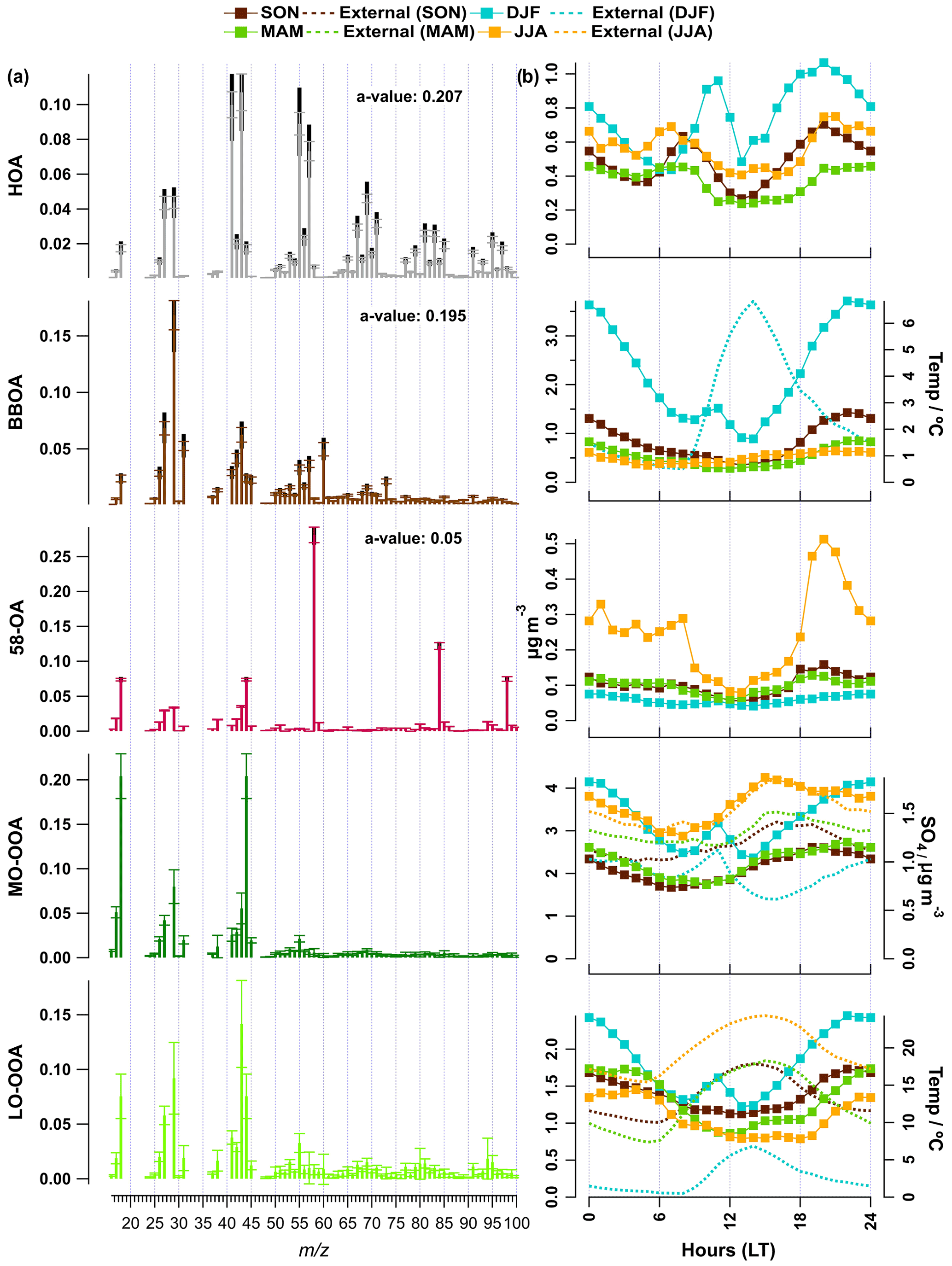
Figure 5Overview of the primary and secondary OA components in Magadino in 2013–2014: (a) OA factor profiles and (b) seasonal diurnal cycles of HOA, BBOA, 58-OA, MO-OOA, and LO-OOA. The ambient temperature is shown in the LO-OOA diurnal plots. In (a) the error bar is the standard deviation; the black bars show the maximum and the minimum that the variable was allowed to vary from the reference profiles. The average, 10th, and 90th percentiles for a values of HOA are 0.195, 0.007, and 0.378, respectively. Also, the average, 10th, and 90th percentiles for a values of BBOA are 0.202, 0.025, and 0.379, respectively.
Due to extensive residential wood combustion combined with winter inversions, the concentrations of BBOA and eBCwb were 3 times higher at night than at midday. As discussed above, during winter, all of the air pollutants, including all PMF factors, peaked concurrently at 10:00–11:00 (local time) due to delayed illumination of the valley site and slow wind speed near the ground (light blue markers in Fig. 2 for total PM1 and Fig. 5b). In summer, additional local photochemical production led to an increasing MO-OOA mass during the day (yellow markers in Fig. 5b), which is similar to the sulfate diurnal behaviour (r2=0.63). A nighttime increase and a daytime decrease in the LO-OOA mass during spring and summer apparently followed condensation and re-evaporation cycles of semi-volatile species, which is similar to the behaviour of ammonium nitrate. Additionally, nocturnal chemistry of NO3 and N2O5 radicals could lead to the formation of HNO3 via N2O5 hydrolysis and of organic nitrates via oxidation of volatile organic compounds (VOCs) (Brown et al., 2004; Dentener and Crutzen, 1993), thus influencing the diurnal cycles of both particulate nitrate and LO-OOA (with r2=0.48 for spring and r2=0.36 for summer).
Figure 6 also presents the diurnal cycles of HOA, eBCtr, and NOx with different patterns for weekdays and weekends. The hourly averages of HOA and eBCtr and the NOx mixing ratio peak during the morning and evening rush hours over the weekdays, while on the weekends, there is only an evening pollution increase coinciding with the time when people come back from holidays or nighttime leisure activities.

Figure 6Diurnal cycles of HOA (grey symbols), black carbon apportioned to traffic emissions eBCtr (dashed lines), and NOx (dotted lines) for weekdays (a) and weekends (b). The shaded areas represent the interquartile range for HOA (1 h averages).
3.3.2 f44–f43 analysis of secondary OA factors
While 44 is mostly from the fragment of CO, a fingerprint of oxygenated species, 43 can originate from C2H3O+ (a fingerprint of semi-volatile species) or C3H (a fingerprint of the primary emissions of hydrocarbon-like species) (Canonaco et al., 2015; Chirico et al., 2010; Ng et al., 2010). Thus, f44 and f43 are often used to identify the oxidation state of the factors, which is crucial to differentiate the MO-OOA and LO-OOA factors. Under the premise that the POA factors and the 58-OA factor are all well resolved, it is essential to investigate the relationship between the 44 and 43 signals in the OOA factors to determine whether or not one/two OOA factors are sufficient to explain the dataset. In addition, the shapes of the yellow and red dots shown in an f44–f43 plot (Fig. 7) may also include some source-related information. Figure 7 depicts the relationship between f44 and f43 of two modelled OOA factors for the different seasons. The yellow cloud of data points represents the measured f44 vs. f43 after subtracting the 44 and 43 signals contributed by the primary HOA, BBOA, and 58-OA factors (Eqs. S11 and S12). They are colour-coded by the total OA mass concentration (data points with OA mass concentration below 2 µg m−3 are hidden).
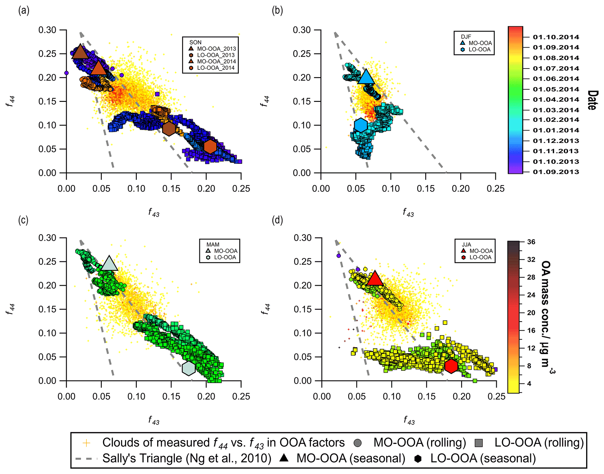
Figure 7The f44 and f43 of OOA (after subtraction of signals contributed by the primary HOA, BBOA, and 58-OA factors) for four different seasons. The small yellow and red crosses of data points represent f44 vs. f43. They are colour-coded by the total OA mass concentration. The bigger sizes of triangles and hexagons represent the ratios between f44 and f43 intensities within the factor profiles of MO-OOA and LO-OOA in seasonal solutions, respectively. The smaller sizes of circles and squares are ratios between f44 and f43 intensities within the factor profiles of MO-OOA and LO-OOA from rolling PMF analysis, which are colour-coded by date and time. The dashed lines represent Sally's triangle from Ng et al. (2010) and depict the region where OOA from multiple PMF analyses during the last decade resided in the f44–f43 space.
As shown in Fig. 7a, the data points in September–October (in both 2013 and 2014) were located on the right side of the triangle first presented by Ng et al. (2010), while the November (2013) data points were located within the triangle. In addition, the spring and summer data points (Fig. 7c and d) were all located instead on the right side of the triangle, but the winter points lay within the triangle (Fig. 7b). We made a similar plot but with a monthly resolution and different colour codes in Fig. S9. The data points located within the triangle correspond to the time with a lower temperature than that of those that are closer to the right side of the triangle in Fig. S9. This could be explained by the increased biogenic OOA contributions when the temperature was higher, as biogenic OOA tends to be distributed along the right side of the triangle (Canonaco et al., 2015; Pfaffenberger et al., 2013). Also, when the temperature decreases, the increased biomass emissions make the OOA points lie vertically within the triangle (Canonaco et al., 2015; Heringa et al., 2011), which is the case for the winter data (Fig. 7b).
In July 2014, the rolling PMF LO-OOA moved towards the left side of the plot due to increasing influences from 80, 94 (C2H6S), 95, and 96 (Fig. S7). Because the OA signal of 80 is directly calculated from 94 (Allan et al., 2004), we did not investigate the sources of 80. In July, a potential source of these distinct ions was some oxidation products of dimethyl disulfide, which show signals at 94, 95, and 96 (NIST Mass Spectrometry Data Center, 2014). Dimethyl disulfide is widely used in pesticides. Considering that the sampling site is in the middle of farmland and the diurnal variation in 94 appeared to peak during the daytime, we considered the LO-OOA in July to be highly affected by agricultural activities. However, the static factor profiles of summer LO-OOA from the seasonal summer solution had much smaller intensities for 80 and 94 (Fig. S4), which enhanced the scaled residuals for these two variables in the seasonal solutions.
In winter, LO-OOA (Fig. 9b) was highly affected by biomass burning emissions characterised by the presence of 60, 73 (Alfarra et al., 2007), and the LO-OOA position in the f44–f43 space moved towards the top-right direction in the plot due to the increasing biogenic influence as the temperature rose (Figs. 7b, S9) (Canonaco et al., 2015).
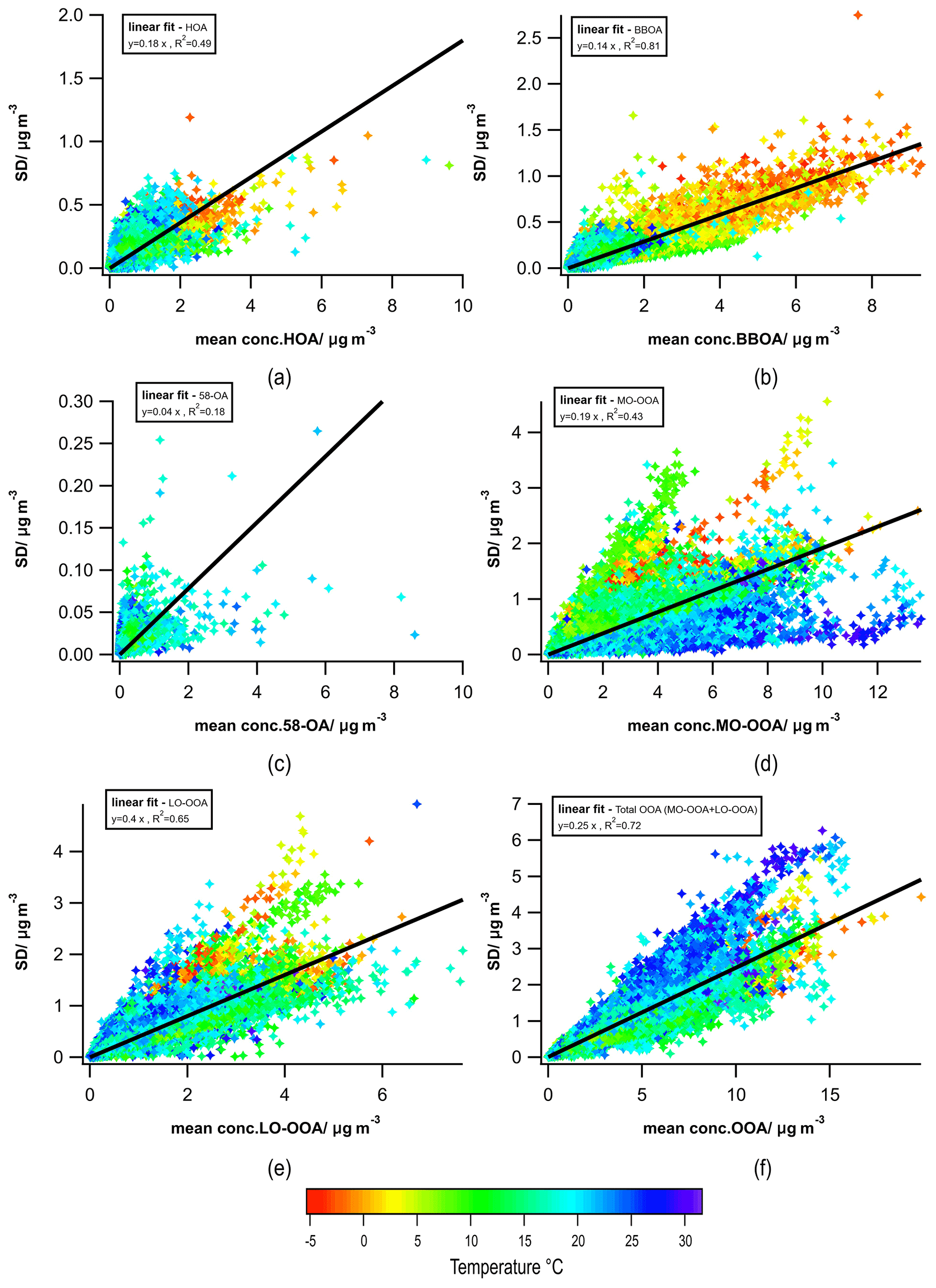
Figure 8Absolute statistical uncertainties in PMF for HOA, BBOA, 58-OA, LO-OOA, MO-OOA, and total OOA (LO-OOA + MO-OOA) for all data. The data points are colour-coded by temperature. The PMF error (uncertainties) of selected PMF runs and rotational uncertainties are estimated using the slope of the linear regression of standard deviation (σ) vs. the averaged mass concentration (μ) for each factor.
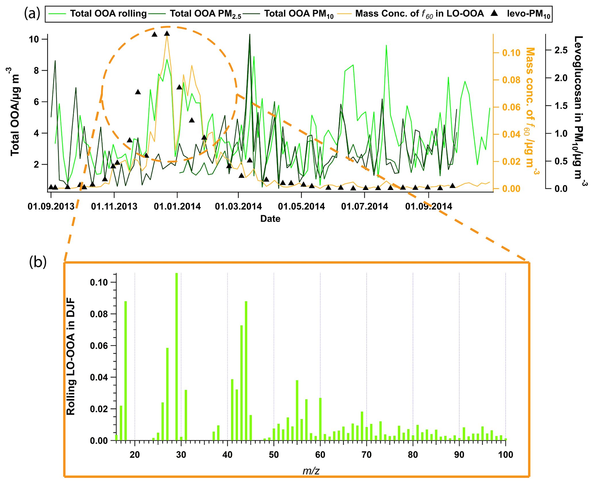
Figure 9(a) Time series of total oxygenated organic aerosol (LO-OOA + MO-OOA) from online and offline source apportionment solutions, together with f60 in LO-OOA for online solutions and levoglucosan in PM10 filters; (b) averaged LO-OOA factor profile from the online solution during DJF (December, January, and February), when online total OOA is significantly higher than that of the offline solution.
Figure 7 also highlights the advantages of rolling PMF over seasonal PMF due to its time-dependent source profiles. Both seasonal and rolling results show that the linear combinations of OOA factors could adequately explain most of the measured OOA points for all the seasons. However, with the static OOA factors for seasonal PMF solutions, it remains challenging to capture the variabilities in some measured data points. In contrast, the rolling PMF OOA factors can move correspondingly with the temporal changes in the clouds, which moves the factor profiles closer to reality and potentially decreases the scaled residuals significantly (Fig. A3). Figure S9 also shows the movements of LO-OOA and MO-OOA factor profiles monthly, where LO-OOA moves towards the right direction as the temperature increases, except for the two light blue squares (June and July) in Fig. S9a. It is clear that temperature plays an important role for the positions of LO-OOA and MO-OOA in the f44–f43 space due to its influences on the OOA sources (biogenic or anthropogenic) as well as the atmospheric processes, which is consistent with previous studies in Zurich (Canonaco et al., 2015).
3.3.3 Statistical and rotational uncertainties
As suggested by Canonaco et al. (2021), combining the bootstrap resampling and the random a-value techniques together with the rolling mechanism, we calculated the standard deviation (σ) and the mean (μ) of the mass concentration for each data point from each OA factor in selected good PMF runs. We estimated the uncertainty in each OA factor using the slope of the linear fit of σ vs. μ (Fig. 8). Since the 58-OA factor was tightly constrained with an a value of 0.05, it had the smallest variability (4 %). Overall, we found relatively smaller errors in HOA, BBOA, and MO-OOA (i.e. 18 %, 14 %, and 19 %, respectively) and an error of 25 % for LO-OOA, which is comparable with the previous study (Canonaco et al., 2021). The errors for both the MO-OOA and the LO-OOA factor showed some temperature dependence. However, this actually varied with time, and the errors did not significantly change when we divided the dataset into four different temperature groups. Still, data points with higher temperature tended to have larger error for the total OOA than with lower temperature (Fig. 8f). This was most likely due to the increase in biogenic emissions and the increasing photochemistry (high O3 and NO2 concentration) at high temperatures (> 20 ∘C), which caused the complexity of the OOA sources.
3.3.4 Online vs. offline
The mass concentrations for HOA, BBOA, and total OOA were compared with corresponding offline AMS results (Vlachou et al., 2018) (Fig. S11). Despite some disagreement during winter (BBOA and total OOA), BBOA showed a high correlation – with the offline results for both PM10 and PM2.5 having r2 values of 0.83 and 0.84, respectively. The correlation for total OOA was somehow lower, with r2 values of 0.31 and 0.46 for the offline results of PM10 and PM2.5 OOA, respectively. Figure 9a shows that the rolling results had a higher OOA concentration during the winter season than the offline PM2.5 and PM10 results, while the rolling results present a lower BBOA concentration during the winter season than the offline PMPM10 results (Fig. S11b). As shown in Fig. 9b, LO-OOA in the rolling results was heavily affected by biomass burning with apparent biomass trace ions (i.e. 60 and 73). The offline results apportioned these biomass-burning-affected LO-OOA to BBOA, whereas the online ACSM measurements with a higher time resolution could capture the fast oxidation process of biomass burning sources. In addition, the rolling PMF technique enabled the LO-OOA factor profile to adapt to the temporal viabilities of OA sources, so the relatively aged biomass burning OA fraction was apportioned into LO-OOA during wintertime by rolling PMF. The yellow line in Fig. 9a depicts the mass concentration of 60 within LO-OOA, which clearly shows significant enhancements during winter and a good agreement with the total OOA time series from the rolling results. Figure S11 shows that HOA did not correlate at all, which is expected because HOA is typically not water-soluble and therefore has a very low recovery rate of 0.11 for the offline AMS technique based on Daellenbach et al. (2016).
In this study, we conducted the first rolling PMF analysis on a 13-month set of ACSM data collected at a rural site in Switzerland. With the help of the small rolling PMF time window and the random a value and bootstrap resampling analysis, we obtained a time-dependent SA result with error estimations. Overall, we resolved a comprehensive five-factor solution with HOA, BBOA, 58-OA, MO-OOA, and LO-OOA. The contribution of HOA was constant during the year (8.1 %–10.1 %), while BBOA showed a clear seasonal variation (8.3 %–27.4 %), which peaked during winter (due to an increased residential-heating source) and contributed least in summer. OOA was a dominant source throughout the year, with a contribution of 71.6 % on a yearly average. However, the biomass burning source had a strong influence on LO-OOA formation in winter. When summing up LO-OOA and BBOA, it makes residential heating a considerable source at Magadino during winter. Therefore, mitigation of residential wood combustion should be considered to reduce PM levels in Magadino and similar locations, especially in winter. Hüglin and Grange (2021) showed that the reduction in residence wood combustion has already shown some effects in PM mitigation in Magadino. However, the biomass burning contribution remains significant in this region.
This paper also provided a recommended criterion list (Table S1) and a novel way to define thresholds with minimum subjective judgements (Student's t test), which could be a leading example for other Source Finder Professional (SoFi Pro) users to conduct rolling PMF. To ensure a good representation of the modelled POA factors and to validate the SA results, we also used the correlations between the PMF factor time series and external data. Both HOA and BBOA agreed well with the corresponding external tracers (NOx, eBCtr, and eBCwb) for the yearly cycles, except for in summer. This is because the aethalometer model for eBC SA has higher uncertainties with smaller eBCwb mass concentrations. Also, NOx could originate from multiple sources in this season. Therefore, we used HOA vs. eBC and EV60,BBOA to justify these two factors in summer. The correlation of HOA vs. eBC had an r2 of 0.28, with an EV60,BBOA of 0.55 in summer. Moreover, the MO-OOA and LO-OOA factors were well correlated with inorganic SO4 and NO3, respectively. The identified primary and secondary OA factor profiles were consistent with the OA factors previously found at various urban, rural, and remote European locations.
This paper assessed the statistical and rotational uncertainties in the PMF solution by combining the bootstrap resampling technique and the random a-value approach. It shows relatively small errors for constrained factors compared with a previous study in Zurich (Canonaco et al., 2021) and comparable errors for the OOA factors.
We also presented a head-to-head comparison between seasonal PMF solutions and the rolling PMF solution. The POA factors showed good agreement between seasonal and rolling PMF solutions, while the OOA factors exhibited greater differences. Overall, the rolling PMF provided slightly better agreements with external tracers, especially between the OOA factors and corresponding inorganic salts. In addition, the rolling PMF results provided a better representation of the measurements by adapting the temporal variations in OOA factors in the f44–f43 space, which also led to much smaller scaled residuals than for the seasonal PMF. Therefore, the rolling PMF is highly useful when the user wishes to better separate OOA factors (especially during cold seasons) and better represent the measurements. In addition, we will also recommend using the rolling PMF to facilitate the analysis of long-term trends of OA sources with some prior knowledge of OA sources. However, it remains challenging to objectively define the transition point to an improved source apportionment for rolling PMF analysis when a different number of OA factors is necessary for different periods. An upcoming paper (Via et al., 2021) will present more details of the comparison between rolling and seasonal results for multiple datasets. The time series of BBOA and total OOA agreed well with those from offline AMS SA results (Vlachou et al., 2018), except for in winter when the offline AMS technique did not capture the fast oxidation processes of biomass burning emissions.
Knowledge of diurnal, seasonal, and annual changes in OA sources is essential for interpreting the yearly cycles of OA and defining mitigation strategies for air quality. With the help of more accurate and realistic OA sources, together with an estimation of the statistical uncertainty in PMF, more constraints can be provided for both climate and air quality models. These improved results are therefore highly valuable for policymakers to solve aerosol-related environmental issues.
The bootstrapped seasonal PMF solutions were compared with the full-year rolling PMF results as follows. The correlations with external data, the ion intensities in the factor profiles, and the mass concentrations retrieved from the two different source apportionment techniques were compared for each factor. The correlations of the factor time series with external data (i.e. NOx, eBCtr, eBCwb, eBCtotal, SO4, NO3, and NH4) are presented in Table A1. The rolling results generally showed slightly better correlations between LO-OOA and NO3, MO-OOA and SO4, and total OOA with NH4 than the seasonal PMF results, which is consistent with the comparison results from Canonaco et al. (2021). A significant improvement was evident for LO-OOA vs. NO3 in spring (with r2 increasing from 0.02 to 0.48). Concerning the correlations of POA factors with external data, rolling results and seasonal results were similar.
Table A1Correlation coefficients () between the factor contributions and expected tracers over the year and for individual meteorological seasons (p<0.05). n/a means not applicable, and the slashes in the first column denote correlations between variables.
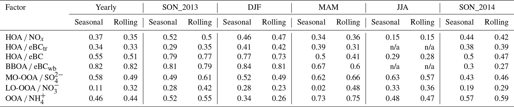
Figure A1 shows a good agreement for two techniques, except for MO-OOA and LO-OOA. In general, the slope of 1.09 for rolling total OOA vs. seasonal OOA suggests the seasonal PMF method tends to apportion more OOA components, while the slope (< 1) for HOA and BBOA suggests that the seasonal PMF technique tends to apportion fewer HOA and BBOA. In addition, 58-OA shows the best agreement between the seasonal and rolling solutions due to the tight constraint of 58-OA with an a value of 0.05.
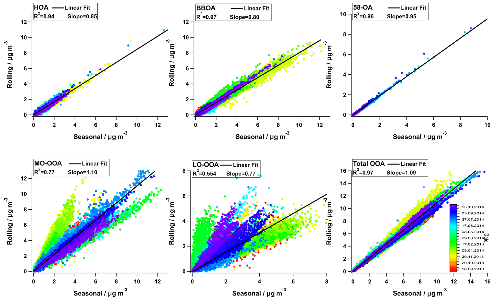
Figure A1Comparison of the mass concentrations resulting from rolling PMF and from the seasonal analysis for each factor (colour-coded by date and time).
The LO-OOA and MO-OOA factors showed worse agreement than the POA factors for the whole dataset. They had good correlations in each meteorological season, however, with different slopes. For instance, seasonal PMF underestimated LO-OOA in spring and autumn 2014, but both seasons showed a high correlation with rather narrow scattering. The over-apportionment of MO-OOA compensated for the under-apportionment of LO-OOA by seasonal PMF for these two seasons. Therefore, the summed OOA still showed a high correlation between rolling and seasonal PMF results. This is expected, as the rolling PMF allows the source profiles to adapt to temporal variations, while seasonal PMF has only static source profiles.
The differences in the major variables of the OOA factors (i.e. 44, 43, and 60) shifted the mass concentrations significantly. Therefore, we also compared the factor profiles for both techniques (Fig. A2). For instance, LO-OOA during spring showed higher intensity at 44 for the rolling PMF results than for the seasonal PMF results (Fig. A2), which caused the underestimation of LO-OOA for the seasonal PMF in spring. When we averaged the total OOA factor using mass-weighted MO-OOA and LO-OOA factors, rolling PMF yielded higher 60 for all seasons. As a result, seasonal PMF apportions slightly fewer summed OOA factors by around 9 %, while it apportions slightly more POA factors within 6 %.
The profiles of the constrained factors (HOA, BBOA, 58-OA) from the rolling results show a very high correlation with the seasonal results (Fig. A2), which suggests that the primary factors and the tightly constrained factor (58-OA) were consistent with the static profiles from the seasonal PMF analysis.
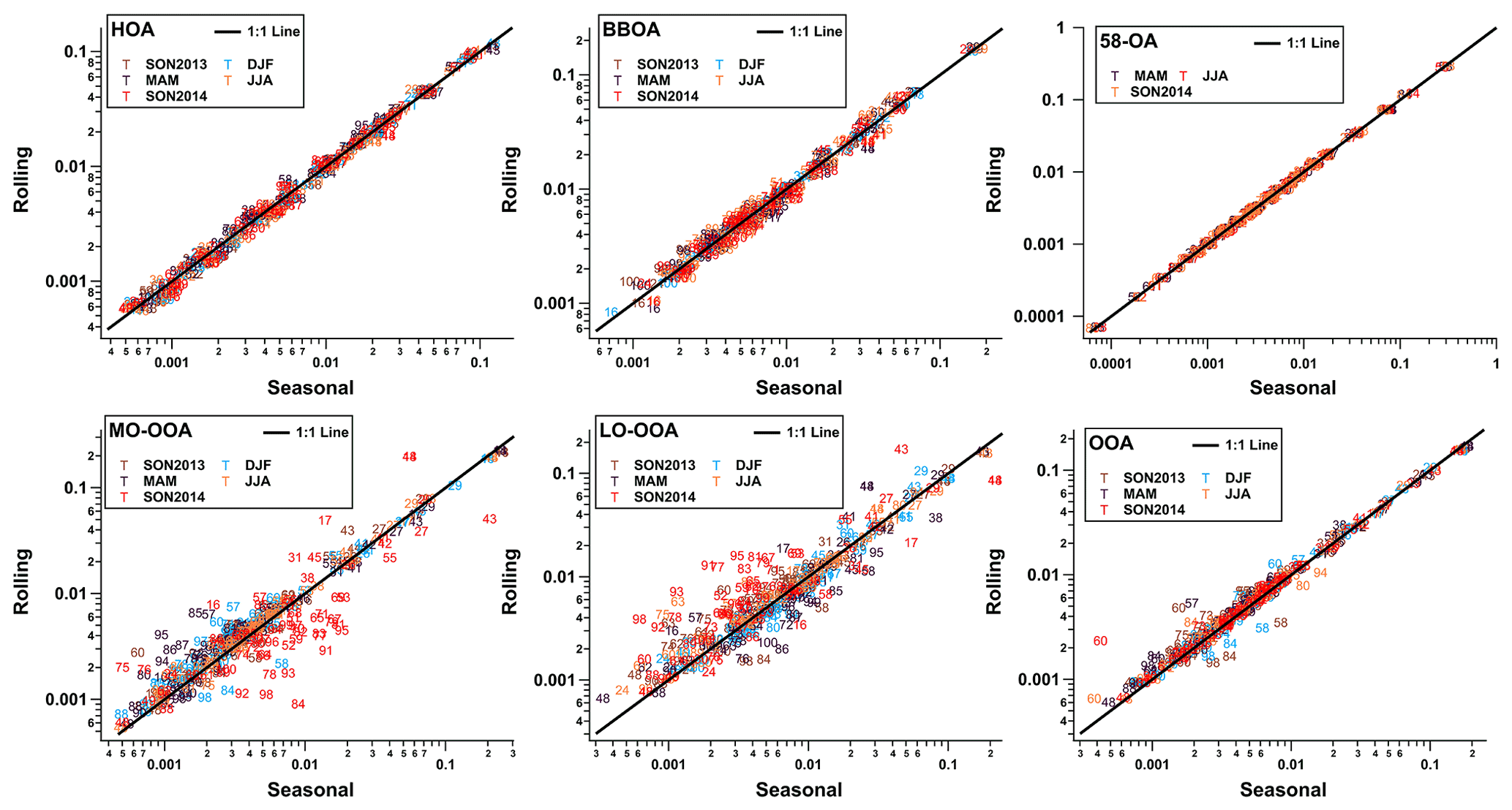
Figure A2Profile comparisons between rolling results and seasonal results for each factor (log scale).
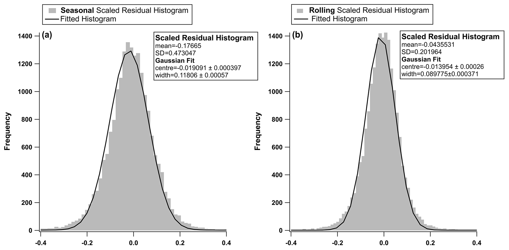
Figure A3Distribution of the scaled residuals over the whole year for the seasonal solution (a) and the rolling solution (b).
We compared the scaled residuals from both source apportionment techniques (Fig. A3). The rolling PMF solution had smaller scaled residuals (narrower histogram and the centre is closer to 0) than those of the seasonal PMF solution, which is expected because rolling PMF had more flexibility to adapt to the temporal variabilities in the OA sources.
Summarising, HOA and BBOA were consistent for rolling and seasonal PMF analysis in terms of the time series, correlations with external tracers, and factor profiles due to the consistency of their chemical factor profiles. In contrast, the MO-OOA and LO-OOA factors were more scattered in averaged factor profiles and mass concentration, suggesting that seasonal PMF analysis was insufficient for capturing these temporal variations in their oxidation processes. Also, rolling PMF showed smaller scaled residuals. Therefore, we conclude that the rolling PMF analysis provides more realistic results than the seasonal analysis.
Data related to this paper are available at https://doi.org/10.5281/zenodo.5113896 (Chen et al., 2021).
The supplement related to this article is available online at: https://doi.org/10.5194/acp-21-15081-2021-supplement.
GC analysed the ACSM and eBC data, performed the rolling source apportionment, and wrote the manuscript. YS wrote the preliminary manuscript and analysed preliminary results. GC, YS, FC, AT, KRD, JGS, IEH, UB, and ASHP helped edit and review the manuscript. YS, RF, and PG helped to run the campaign. PG and CH provided external data to validate PMF solutions. FC provided technical support for SoFi Pro. FC, AT, KRD, AV, JGS, IEH, UB, and ASHP participated in discussions for this study.
Yulia Sosedova, Francesco Canonaco, Anna Tobler, Carlo Bozzetti are working for Datalystica Ltd., the company that developed the SoFi Pro software. All authors declare no competing interests in any form for this work.
Publisher's note: Copernicus Publications remains neutral with regard to jurisdictional claims in published maps and institutional affiliations.
The ACSM measurements were supported by the Swiss Federal Office for the Environment (FOEN). The leading role of the Laboratory for Air Pollution and Environmental Technology of the Swiss Federal Laboratories for Materials and Testing (Empa) in supporting the measurements is very much appreciated. Yulia Sosedova acknowledges support by the Wiedereinsteigerinnen-Programm at the Paul Scherrer Institute. This study was also supported by the COST Action of Chemical On-Line cOmpoSition and Source Apportionment of fine aerosoL (COLOSSAL, CA16109).
This research has been supported by the European Research Council, H2020 European Research Council (ERA-PLANET (grant no. 689443)) and a COST-related project of the Swiss National Science Foundation, the Schweizerischer Nationalfonds zur Förderung der Wissenschaftlichen Forschung (SAMSAM (grant no. IZCOZ0_177063)).
This paper was edited by Maria Cristina Facchini and reviewed by three anonymous referees.
Aiken, A. C., Salcedo, D., Cubison, M. J., Huffman, J. A., DeCarlo, P. F., Ulbrich, I. M., Docherty, K. S., Sueper, D., Kimmel, J. R., Worsnop, D. R., Trimborn, A., Northway, M., Stone, E. A., Schauer, J. J., Volkamer, R. M., Fortner, E., de Foy, B., Wang, J., Laskin, A., Shutthanandan, V., Zheng, J., Zhang, R., Gaffney, J., Marley, N. A., Paredes-Miranda, G., Arnott, W. P., Molina, L. T., Sosa, G., and Jimenez, J. L.: Mexico City aerosol analysis during MILAGRO using high resolution aerosol mass spectrometry at the urban supersite (T0) – Part 1: Fine particle composition and organic source apportionment, Atmos. Chem. Phys., 9, 6633–6653, https://doi.org/10.5194/acp-9-6633-2009, 2009.
Alfarra, M. R., Prevot, A. S. H., Szidat, S., Sandradewi, J., Weimer, S., Lanz, V. A., Schreiber, D., Mohr, M., and Baltensperger, U.: Identification of the Mass Spectral Signature of Organic Aerosols from Wood Burning Emissions, Environ. Sci. Technol., 41, 5770–5777, https://doi.org/10.1021/es062289b, 2007.
Allan, J. D., Alfarra, M. R., Bower, K. N., Williams, P. I., Gallagher, M. W., Jimenez, J. L., McDonald, A. G., Nemitz, E., Canagaratna, M. R., Jayne, J. T., Coe, H., and Worsnop, D. R.: Quantitative sampling using an Aerodyne aerosol mass spectrometer 2. Measurements of fine particulate chemical composition in two U.K. cities, J. Geophys. Res.-Atmos., 108, 4091, https://doi.org/10.1029/2002JD002359, 2003.
Allan, J. D., Delia, A. E., Coe, H., Bower, K. N., Alfarra, M. R. R., Jimenez, J. L., Middlebrook, A. M., Drewnick, F., Onasch, T. B., Canagaratna, M. R., Jayne, J. T., and Worsnop, D. R.: A generalised method for the extraction of chemically resolved mass spectra from Aerodyne aerosol mass spectrometer data, J. Aerosol Sci., 35, 909–922, https://doi.org/10.1016/j.jaerosci.2004.02.007, 2004.
Bressi, M., Cavalli, F., Belis, C. A., Putaud, J.-P., Fröhlich, R., Martins dos Santos, S., Petralia, E., Prévôt, A. S. H., Berico, M., Malaguti, A., and Canonaco, F.: Variations in the chemical composition of the submicron aerosol and in the sources of the organic fraction at a regional background site of the Po Valley (Italy), Atmos. Chem. Phys., 16, 12875–12896, https://doi.org/10.5194/acp-16-12875-2016, 2016.
Brown, S. S., Dibb, J. E., Stark, H., Aldener, M., Vozella, M., Whitlow, S., Williams, E. J., Lerner, B. M., Jakoubek, R., Middlebrook, A. M., DeGouw, J. A., Warneke, C., Goldan, P. D., Kuster, W. C., Angevine, W. M., Sueper, D. T., Quinn, P. K., Bates, T. S., Meagher, J. F., Fehsenfeld, F. C., and Ravishankara, A. R.: Nighttime removal of NOx in the summer marine boundary layer, Geophys. Res. Lett., 31, L07108, https://doi.org/10.1029/2004GL019412, 2004.
Canagaratna, M. R., Jayne, J. T., Jimenez, J. L., Allan, J. D., Alfarra, M. R., Zhang, Q., Onasch, T. B., Drewnick, F., Coe, H., Middlebrook, A., Delia, A., Williams, L. R., Trimborn, A. M., Northway, M. J., DeCarlo, P. F., Kolb, C. E., Davidovits, P., and Worsnop, D. R.: Chemical and microphysical characterisation of ambient aerosols with the aerodyne aerosol mass spectrometer, Mass Spectrom. Rev., 26, 185–222, https://doi.org/10.1002/mas.20115, 2007.
Canonaco, F., Crippa, M., Slowik, J. G., Baltensperger, U., and Prévôt, A. S. H.: SoFi, an IGOR-based interface for the efficient use of the generalized multilinear engine (ME-2) for the source apportionment: ME-2 application to aerosol mass spectrometer data, Atmos. Meas. Tech., 6, 3649–3661, https://doi.org/10.5194/amt-6-3649-2013, 2013.
Canonaco, F., Slowik, J. G., Baltensperger, U., and Prévôt, A. S. H.: Seasonal differences in oxygenated organic aerosol composition: implications for emissions sources and factor analysis, Atmos. Chem. Phys., 15, 6993–7002, https://doi.org/10.5194/acp-15-6993-2015, 2015.
Canonaco, F., Tobler, A., Chen, G., Sosedova, Y., Slowik, J. G., Bozzetti, C., Daellenbach, K. R., El Haddad, I., Crippa, M., Huang, R.-J., Furger, M., Baltensperger, U., and Prévôt, A. S. H.: A new method for long-term source apportionment with time-dependent factor profiles and uncertainty assessment using SoFi Pro: application to 1 year of organic aerosol data, Atmos. Meas. Tech., 14, 923–943, https://doi.org/10.5194/amt-14-923-2021, 2021.
Chen, G., Sosedva, Y., Canonaco, F., Fröhlich, R., Tobler, A., Vlachou, A., Daellenbach, K. R., Bozzetti, C., Hueglin, C., Graf, P., Baltensperger, U., Slowik, J. G., Haddad, I. E., and Prévôt, A. S. H.: Dataset: Time dependent source apportionment of submicron organic aerosol for a rural site in an alpine valley using a rolling PMF window (Version 1st), Zenodo [data set], https://doi.org/10.5281/zenodo.5113896, 2021.
Chirico, R., DeCarlo, P. F., Heringa, M. F., Tritscher, T., Richter, R., Prévôt, A. S. H., Dommen, J., Weingartner, E., Wehrle, G., Gysel, M., Laborde, M., and Baltensperger, U.: Impact of aftertreatment devices on primary emissions and secondary organic aerosol formation potential from in-use diesel vehicles: results from smog chamber experiments, Atmos. Chem. Phys., 10, 11545–11563, https://doi.org/10.5194/acp-10-11545-2010, 2010.
Chow, J. C., Bachmann, J. D., Wierman, S. S. G., Mathai, C. V., Malm, W. C., White, W. H., Mueller, P. K., Kumar, N., and Watson, J. G.: Visibility: Science and Regulation, J. Air Waste Manage., 52, 973–999, https://doi.org/10.1080/10473289.2002.10470844, 2002.
Crippa, M., DeCarlo, P. F., Slowik, J. G., Mohr, C., Heringa, M. F., Chirico, R., Poulain, L., Freutel, F., Sciare, J., Cozic, J., Di Marco, C. F., Elsasser, M., Nicolas, J. B., Marchand, N., Abidi, E., Wiedensohler, A., Drewnick, F., Schneider, J., Borrmann, S., Nemitz, E., Zimmermann, R., Jaffrezo, J.-L., Prévôt, A. S. H., and Baltensperger, U.: Wintertime aerosol chemical composition and source apportionment of the organic fraction in the metropolitan area of Paris, Atmos. Chem. Phys., 13, 961–981, https://doi.org/10.5194/acp-13-961-2013, 2013.
Crippa, M., Canonaco, F., Lanz, V. A., Äijälä, M., Allan, J. D., Carbone, S., Capes, G., Ceburnis, D., Dall'Osto, M., Day, D. A., DeCarlo, P. F., Ehn, M., Eriksson, A., Freney, E., Hildebrandt Ruiz, L., Hillamo, R., Jimenez, J. L., Junninen, H., Kiendler-Scharr, A., Kortelainen, A.-M., Kulmala, M., Laaksonen, A., Mensah, A. A., Mohr, C., Nemitz, E., O'Dowd, C., Ovadnevaite, J., Pandis, S. N., Petäjä, T., Poulain, L., Saarikoski, S., Sellegri, K., Swietlicki, E., Tiitta, P., Worsnop, D. R., Baltensperger, U., and Prévôt, A. S. H.: Organic aerosol components derived from 25 AMS data sets across Europe using a consistent ME-2 based source apportionment approach, Atmos. Chem. Phys., 14, 6159–6176, https://doi.org/10.5194/acp-14-6159-2014, 2014.
Cubison, M. J., Ortega, A. M., Hayes, P. L., Farmer, D. K., Day, D., Lechner, M. J., Brune, W. H., Apel, E., Diskin, G. S., Fisher, J. A., Fuelberg, H. E., Hecobian, A., Knapp, D. J., Mikoviny, T., Riemer, D., Sachse, G. W., Sessions, W., Weber, R. J., Weinheimer, A. J., Wisthaler, A., and Jimenez, J. L.: Effects of aging on organic aerosol from open biomass burning smoke in aircraft and laboratory studies, Atmos. Chem. Phys., 11, 12049–12064, https://doi.org/10.5194/acp-11-12049-2011, 2011.
Daellenbach, K. R., Bozzetti, C., Křepelová, A., Canonaco, F., Wolf, R., Zotter, P., Fermo, P., Crippa, M., Slowik, J. G., Sosedova, Y., Zhang, Y., Huang, R.-J., Poulain, L., Szidat, S., Baltensperger, U., El Haddad, I., and Prévôt, A. S. H.: Characterization and source apportionment of organic aerosol using offline aerosol mass spectrometry, Atmos. Meas. Tech., 9, 23–39, https://doi.org/10.5194/amt-9-23-2016, 2016.
Daellenbach, K. R., Uzu, G., Jiang, J., Cassagnes, L.-E., Leni, Z., Vlachou, A., Stefenelli, G., Canonaco, F., Weber, S., Segers, A., Kuenen, J. J. P., Schaap, M., Favez, O., Albinet, A., Aksoyoglu, S., Dommen, J., Baltensperger, U., Geiser, M., El Haddad, I., Jaffrezo, J.-L., and Prévôt, A. S. H.: Sources of particulate-matter air pollution and its oxidative potential in Europe, Nature, 587, 414–419, https://doi.org/10.1038/s41586-020-2902-8, 2020.
DeCarlo, P. F., Dunlea, E. J., Kimmel, J. R., Aiken, A. C., Sueper, D., Crounse, J., Wennberg, P. O., Emmons, L., Shinozuka, Y., Clarke, A., Zhou, J., Tomlinson, J., Collins, D. R., Knapp, D., Weinheimer, A. J., Montzka, D. D., Campos, T., and Jimenez, J. L.: Fast airborne aerosol size and chemistry measurements above Mexico City and Central Mexico during the MILAGRO campaign, Atmos. Chem. Phys., 8, 4027–4048, https://doi.org/10.5194/acp-8-4027-2008, 2008.
Dentener, F. J. and Crutzen, P. J.: Reaction of N2O5 on tropospheric aerosols: Impact on the global distributions of NOx, O3, and OH, J. Geophys. Res.-Atmos., 98, 7149–7163, https://doi.org/10.1029/92JD02979, 1993.
Dockery, D. W. and Pope, C. A.: Acute Respiratory Effects of Particulate Air Pollution, Annu. Rev. Publ. Hlth., 15, 107–132, https://doi.org/10.1146/annurev.pu.15.050194.000543, 1994.
Duplissy, J., DeCarlo, P. F., Dommen, J., Alfarra, M. R., Metzger, A., Barmpadimos, I., Prevot, A. S. H., Weingartner, E., Tritscher, T., Gysel, M., Aiken, A. C., Jimenez, J. L., Canagaratna, M. R., Worsnop, D. R., Collins, D. R., Tomlinson, J., and Baltensperger, U.: Relating hygroscopicity and composition of organic aerosol particulate matter, Atmos. Chem. Phys., 11, 1155–1165, https://doi.org/10.5194/acp-11-1155-2011, 2011.
Efron, B.: Bootstrap Methods: Another Look at the Jackknife, Ann. Stat., 7, 1–26, 1979.
Fröhlich, R., Cubison, M. J., Slowik, J. G., Bukowiecki, N., Prévôt, A. S. H., Baltensperger, U., Schneider, J., Kimmel, J. R., Gonin, M., Rohner, U., Worsnop, D. R., and Jayne, J. T.: The ToF-ACSM: a portable aerosol chemical speciation monitor with TOFMS detection, Atmos. Meas. Tech., 6, 3225–3241, https://doi.org/10.5194/amt-6-3225-2013, 2013.
Fröhlich, R., Crenn, V., Setyan, A., Belis, C. A., Canonaco, F., Favez, O., Riffault, V., Slowik, J. G., Aas, W., Aijälä, M., Alastuey, A., Artiñano, B., Bonnaire, N., Bozzetti, C., Bressi, M., Carbone, C., Coz, E., Croteau, P. L., Cubison, M. J., Esser-Gietl, J. K., Green, D. C., Gros, V., Heikkinen, L., Herrmann, H., Jayne, J. T., Lunder, C. R., Minguillón, M. C., Močnik, G., O'Dowd, C. D., Ovadnevaite, J., Petralia, E., Poulain, L., Priestman, M., Ripoll, A., Sarda-Estève, R., Wiedensohler, A., Baltensperger, U., Sciare, J., and Prévôt, A. S. H.: ACTRIS ACSM intercomparison – Part 2: Intercomparison of ME-2 organic source apportionment results from 15 individual, co-located aerosol mass spectrometers, Atmos. Meas. Tech., 8, 2555–2576, https://doi.org/10.5194/amt-8-2555-2015, 2015.
Heringa, M. F., DeCarlo, P. F., Chirico, R., Tritscher, T., Dommen, J., Weingartner, E., Richter, R., Wehrle, G., Prévôt, A. S. H., and Baltensperger, U.: Investigations of primary and secondary particulate matter of different wood combustion appliances with a high-resolution time-of-flight aerosol mass spectrometer, Atmos. Chem. Phys., 11, 5945–5957, https://doi.org/10.5194/acp-11-5945-2011, 2011.
Hildebrandt, L., Kostenidou, E., Lanz, V. A., Prevot, A. S. H., Baltensperger, U., Mihalopoulos, N., Laaksonen, A., Donahue, N. M., and Pandis, S. N.: Sources and atmospheric processing of organic aerosol in the Mediterranean: insights from aerosol mass spectrometer factor analysis, Atmos. Chem. Phys., 11, 12499–12515, https://doi.org/10.5194/acp-11-12499-2011, 2011.
Horvath, H.: Atmospheric light absorption – A review, Atmos. Environ., 27, 293–317, https://doi.org/10.1016/0960-1686(93)90104-7, 1993.
Hüglin, C. and Grange, S. K.: Chemical characterisation and source identification, Dübendorf, Zurich, available at: https://www.aramis.admin.ch/Default?DocumentID=67473&Load=true, last access: 20 July 2021.
IPCC: Clouds and Aerosols, in: Climate Change 2013 – The Physical Science Basis, edited by Intergovernmental Panel on Climate Change, Cambridge University Press, Cambridge, 571–658, 2014.
Jacobson, M. C., Hansson, H.-C., Noone, K. J., and Charlson, R. J.: Organic atmospheric aerosols: Review and state of the science, Rev. Geophys., 38, 267–294, https://doi.org/10.1029/1998RG000045, 2000.
Jacobson, M. Z.: Global direct radiative forcing due to multicomponent anthropogenic and natural aerosols, J. Geophys. Res.-Atmos., 106, 1551–1568, https://doi.org/10.1029/2000JD900514, 2001.
Jimenez, J. L., Canagaratna, M. R., Donahue, N. M., Prevot, A. S. H. H., Zhang, Q., Kroll, J. H., DeCarlo, P. F., Allan, J. D., Coe, H., Ng, N. L., Aiken, A. C., Docherty, K. S., Ulbrich, I. M., Grieshop, A. P., Robinson, A. L., Duplissy, J., Smith, J. D., Wilson, K. R., Lanz, V. A., Hueglin, C., Sun, Y. L., Tian, J., Laaksonen, A., Raatikainen, T., Rautiainen, J., Vaattovaara, P., Ehn, M., Kulmala, M., Tomlinson, J. M., Collins, D. R., Cubison, M. J., Dunlea, J., Huffman, J. A., Onasch, T. B., Alfarra, M. R., Williams, P. I., Bower, K., Kondo, Y., Schneider, J., Drewnick, F., Borrmann, S., Weimer, S., Demerjian, K., Salcedo, D., Cottrell, L., Griffin, R., Takami, A., Miyoshi, T., Hatakeyama, S., Shimono, A., Sun, J. Y., Zhang, Y. M., Dzepina, K., Kimmel, J. R., Sueper, D., Jayne, J. T., Herndon, S. C., Trimborn, A. M., Williams, L. R., Wood, E. C., Middlebrook, A. M., Kolb, C. E., Baltensperger, U., and Worsnop, D. R.: Evolution of organic aerosols in the atmosphere, Science, 326, 1525–1529, https://doi.org/10.1126/science.1180353, 2009.
Lanz, V. A., Alfarra, M. R., Baltensperger, U., Buchmann, B., Hueglin, C., and Prévôt, A. S. H.: Source apportionment of submicron organic aerosols at an urban site by factor analytical modelling of aerosol mass spectra, Atmos. Chem. Phys., 7, 1503–1522, https://doi.org/10.5194/acp-7-1503-2007, 2007.
Lanz, V. A., Alfarra, M. R., Baltensperger, U., Buchmann, B., Hueglin, C., Szidat, S., Wehrli, M. N., Wacker, L., Weimer, S., Caseiro, A., Puxbaum, H., and Prevot, A. S. H.: Source Attribution of Submicron Organic Aerosols during Wintertime Inversions by Advanced Factor Analysis of Aerosol Mass Spectra, Environ. Sci. Technol., 42, 214–220, https://doi.org/10.1021/es0707207, 2008.
Lelieveld, J., Evans, J. S., Fnais, M., Giannadaki, D., and Pozzer, A.: The contribution of outdoor air pollution sources to premature mortality on a global scale, Nature, 525, 367–371, https://doi.org/10.1038/nature15371, 2015.
Matthew, B. M., Middlebrook, A. M., and Onasch, T. B.: Collection Efficiencies in an Aerodyne Aerosol Mass Spectrometer as a Function of Particle Phase for Laboratory Generated Aerosols, Aerosol Sci. Tech., 42, 884–898, https://doi.org/10.1080/02786820802356797, 2008.
Mauderly, J. L. and Chow, J. C.: Health Effects of Organic Aerosols, Inhal. Toxicol., 20, 257–288, https://doi.org/10.1080/08958370701866008, 2008.
Meteotest: Data Report Switzerland 2007–2016, Bern, Switzerland, 2017.
Minguillón, M. C., Ripoll, A., Pérez, N., Prévôt, A. S. H., Canonaco, F., Querol, X., and Alastuey, A.: Chemical characterization of submicron regional background aerosols in the western Mediterranean using an Aerosol Chemical Speciation Monitor, Atmos. Chem. Phys., 15, 6379–6391, https://doi.org/10.5194/acp-15-6379-2015, 2015.
Mohr, C., DeCarlo, P. F., Heringa, M. F., Chirico, R., Slowik, J. G., Richter, R., Reche, C., Alastuey, A., Querol, X., Seco, R., Peñuelas, J., Jiménez, J. L., Crippa, M., Zimmermann, R., Baltensperger, U., and Prévôt, A. S. H.: Identification and quantification of organic aerosol from cooking and other sources in Barcelona using aerosol mass spectrometer data, Atmos. Chem. Phys., 12, 1649–1665, https://doi.org/10.5194/acp-12-1649-2012, 2012.
Monn, C.: Exposure assessment of air pollutants: a review on spatial heterogeneity and indoor/outdoor/personal exposure to suspended particulate matter, nitrogen dioxide and ozone, Atmos. Environ., 35, 1–32, https://doi.org/10.1016/S1352-2310(00)00330-7, 2001.
Murphy, D. M., Cziczo, D. J., Froyd, K. D., Hudson, P. K., Matthew, B. M., Middlebrook, A. M., Peltier, R. E., Sullivan, A., Thomson, D. S., and Weber, R. J.: Single-particle mass spectrometry of tropospheric aerosol particles, J. Geophys. Res.-Atmos., 111, D23S32, https://doi.org/10.1029/2006JD007340, 2006.
Ng, N. L., Canagaratna, M. R., Zhang, Q., Jimenez, J. L., Tian, J., Ulbrich, I. M., Kroll, J. H., Docherty, K. S., Chhabra, P. S., Bahreini, R., Murphy, S. M., Seinfeld, J. H., Hildebrandt, L., Donahue, N. M., DeCarlo, P. F., Lanz, V. A., Prévôt, A. S. H., Dinar, E., Rudich, Y., and Worsnop, D. R.: Organic aerosol components observed in Northern Hemispheric datasets from Aerosol Mass Spectrometry, Atmos. Chem. Phys., 10, 4625–4641, https://doi.org/10.5194/acp-10-4625-2010, 2010.
Ng, N. L., Herndon, S. C., Trimborn, A., Canagaratna, M. R., Croteau, P. L., Onasch, T. B., Sueper, D., Worsnop, D. R., Zhang, Q., Sun, Y. L., and Jayne, J. T.: An Aerosol Chemical Speciation Monitor (ACSM) for Routine Monitoring of the Composition and Mass Concentrations of Ambient Aerosol, Aerosol Sci. Technol., 45, 780–794, https://doi.org/10.1080/02786826.2011.560211, 2011a.
Ng, N. L., Canagaratna, M. R., Jimenez, J. L., Zhang, Q., Ulbrich, I. M., and Worsnop, D. R.: Real-Time Methods for Estimating Organic Component Mass Concentrations from Aerosol Mass Spectrometer Data, Environ. Sci. Technol., 45, 910–916, https://doi.org/10.1021/es102951k, 2011b.
NIST Mass Spectrometry Data Center: Disulfide, dimethyl, SRD 69, available at: https://webbook.nist.gov/cgi/cbook.cgi?ID=C624920&Mask=200#Refs (last access: 6 August 2020), 2014.
Paatero, P.: The Multilinear Engine – A Table-Driven, Least Squares Program for Solving Multilinear Problems, Including the n-Way Parallel Factor Analysis Model, J. Comput. Graph. Stat., 8, 854–888, https://doi.org/10.1080/10618600.1999.10474853, 1999.
Paatero, P. and Hopke, P. K.: Discarding or downweighting high-noise variables in factor analytic models, Anal. Chim. Acta, 490, 277–289, https://doi.org/10.1016/S0003-2670(02)01643-4, 2003.
Paatero, P., Eberly, S., Brown, S. G., and Norris, G. A.: Methods for estimating uncertainty in factor analytic solutions, Atmos. Meas. Tech., 7, 781–797, https://doi.org/10.5194/amt-7-781-2014, 2014.
Parworth, C., Fast, J., Mei, F., Shippert, T., Sivaraman, C., Tilp, A., Watson, T., and Zhang, Q.: Long-term measurements of submicrometer aerosol chemistry at the Southern Great Plains (SGP) using an Aerosol Chemical Speciation Monitor (ACSM), Atmos. Environ., 106, 43–55, https://doi.org/10.1016/j.atmosenv.2015.01.060, 2015.
Petit, J.-E., Favez, O., Sciare, J., Canonaco, F., Croteau, P., Močnik, G., Jayne, J., Worsnop, D., and Leoz-Garziandia, E.: Submicron aerosol source apportionment of wintertime pollution in Paris, France by double positive matrix factorization (PMF2) using an aerosol chemical speciation monitor (ACSM) and a multi-wavelength Aethalometer, Atmos. Chem. Phys., 14, 13773–13787, https://doi.org/10.5194/acp-14-13773-2014, 2014.
Pfaffenberger, L., Barmet, P., Slowik, J. G., Praplan, A. P., Dommen, J., Prévôt, A. S. H., and Baltensperger, U.: The link between organic aerosol mass loading and degree of oxygenation: an α-pinene photooxidation study, Atmos. Chem. Phys., 13, 6493–6506, https://doi.org/10.5194/acp-13-6493-2013, 2013.
Pope, C. A. and Dockery, D. W.: Health Effects of Fine Particulate Air Pollution: Lines that Connect, J. Air Waste Manage., 56, 709–742, https://doi.org/10.1080/10473289.2006.10464485, 2006.
Ramanathan, V., Chung, C., Kim, D., Bettge, T., Buja, L., Kiehl, J. T., Washington, W. M., Fu, Q., Sikka, D. R., and Wild, M.: Atmospheric brown clouds: Impacts on South Asian climate and hydrological cycle, P. Natl. Acad. Sci. USA, 102, 5326–5333, https://doi.org/10.1073/pnas.0500656102, 2005.
Reyes-Villegas, E., Green, D. C., Priestman, M., Canonaco, F., Coe, H., Prévôt, A. S. H., and Allan, J. D.: Organic aerosol source apportionment in London 2013 with ME-2: exploring the solution space with annual and seasonal analysis, Atmos. Chem. Phys., 16, 15545–15559, https://doi.org/10.5194/acp-16-15545-2016, 2016.
Ripoll, A., Minguillón, M. C., Pey, J., Jimenez, J. L., Day, D. A., Sosedova, Y., Canonaco, F., Prévôt, A. S. H., Querol, X., and Alastuey, A.: Long-term real-time chemical characterization of submicron aerosols at Montsec (southern Pyrenees, 1570 m a.s.l.), Atmos. Chem. Phys., 15, 2935–2951, https://doi.org/10.5194/acp-15-2935-2015, 2015.
Schurman, M. I., Lee, T., Sun, Y., Schichtel, B. A., Kreidenweis, S. M., and Collett Jr., J. L.: Investigating types and sources of organic aerosol in Rocky Mountain National Park using aerosol mass spectrometry, Atmos. Chem. Phys., 15, 737–752, https://doi.org/10.5194/acp-15-737-2015, 2015.
Schwarz, J. P., Gao, R. S., Perring, A. E., Spackman, J. R., and Fahey, D. W.: Black carbon aerosol size in snow, Sci. Rep., 3, 1–5, https://doi.org/10.1038/srep01356, 2013.
Sug Park, E., Henry, R. C., and Spiegelman, C. H.: Estimating the number of factors to include in a high-dimensional multivariate bilinear model, Commun. Stat. Simul. Comput., 29, 723–746, https://doi.org/10.1080/03610910008813637, 2000.
Szidat, S., Prévôt, A. S. H., Sandradewi, J., Alfarra, M. R., Synal, H.-A., Wacker, L., and Baltensperger, U.: Dominant impact of residential wood burning on particulate matter in Alpine valleys during winter, Geophys. Res. Lett., 34, L05820, https://doi.org/10.1029/2006GL028325, 2007.
The Swiss Federal Council: Ordinance of 16 December 1985 on Air Pollution Control (OAPC), available at: https://www.admin.ch/opc/en/classified-compilation/19850321/index.html#app7 (last access: 10 September 2019), 2018.
Tobler, A., Bhattu, D., Canonaco, F., Lalchandani, V., Shukla, A., Thamban, N. M., Mishra, S., Srivastava, A. K., Bisht, D. S., Tiwari, S., Singh, S., Močnik, G., Baltensperger, U., Tripathi, S. N., Slowik, J. G., and Prévôt, A. S. H.: Chemical characterisation of PM2.5 and source apportionment of organic aerosol in New Delhi, India, Sci. Total Environ., 745, 140924, https://doi.org/10.1016/j.scitotenv.2020.140924, 2020.
Ulbrich, I. M., Canagaratna, M. R., Zhang, Q., Worsnop, D. R., and Jimenez, J. L.: Interpretation of organic components from Positive Matrix Factorization of aerosol mass spectrometric data, Atmos. Chem. Phys., 9, 2891–2918, https://doi.org/10.5194/acp-9-2891-2009, 2009.
Via, M., Chen, G., Canonaco, F., Slowik, J. G., Dallenbach, K. R., Prevôt, A. S. H., Alastuey, A., and Minguillón, M. C.: Comparison between rolling and seasonal PMF techniques for organic aerosol source apportionment, in preparation, 2021.
Vlachou, A., Daellenbach, K. R., Bozzetti, C., Chazeau, B., Salazar, G. A., Szidat, S., Jaffrezo, J.-L., Hueglin, C., Baltensperger, U., Haddad, I. E., and Prévôt, A. S. H.: Advanced source apportionment of carbonaceous aerosols by coupling offline AMS and radiocarbon size-segregated measurements over a nearly 2-year period, Atmos. Chem. Phys., 18, 6187–6206, https://doi.org/10.5194/acp-18-6187-2018, 2018.
von Schneidemesser, E., Monks, P. S., Allan, J. D., Bruhwiler, L., Forster, P., Fowler, D., Lauer, A., Morgan, W. T., Paasonen, P., Righi, M., Sindelarova, K., and Sutton, M. A.: Chemistry and the Linkages between Air Quality and Climate Change, Chem. Rev., 115, 3856–3897, https://doi.org/10.1021/acs.chemrev.5b00089, 2015.
Zhang, Q., Jimenez, J. L., Canagaratna, M. R., Allan, J. D., Coe, H., Ulbrich, I., Alfarra, M. R., Takami, A., Middlebrook, A. M., Sun, Y. L., Dzepina, K., Dunlea, E., Docherty, K., DeCarlo, P. F., Salcedo, D., Onasch, T., Jayne, J. T., Miyoshi, T., Shimono, A., Hatakeyama, S., Takegawa, N., Kondo, Y., Schneider, J., Drewnick, F., Borrmann, S., Weimer, S., Demerjian, K., Williams, P., Bower, K., Bahreini, R., Cottrell, L., Griffin, R. J., Rautiainen, J., Sun, J. Y., Zhang, Y. M., and Worsnop, D. R.: Ubiquity and dominance of oxygenated species in organic aerosols in anthropogenically-influenced Northern Hemisphere midlatitudes, Geophys. Res. Lett., 34, https://doi.org/10.1029/2007GL029979, 2007.
Zhang, Q., Jimenez, J. L., Canagaratna, M. R., Ulbrich, I. M., Ng, N. L., Worsnop, D. R., and Sun, Y.: Understanding atmospheric organic aerosols via factor analysis of aerosol mass spectrometry: a review, Anal. Bioanal. Chem., 401, 3045–3067, https://doi.org/10.1007/s00216-011-5355-y, 2011.
Zhang, Y., Favez, O., Petit, J.-E., Canonaco, F., Truong, F., Bonnaire, N., Crenn, V., Amodeo, T., Prévôt, A. S. H., Sciare, J., Gros, V., and Albinet, A.: Six-year source apportionment of submicron organic aerosols from near-continuous highly time-resolved measurements at SIRTA (Paris area, France), Atmos. Chem. Phys., 19, 14755–14776, https://doi.org/10.5194/acp-19-14755-2019, 2019.
Zotter, P., Herich, H., Gysel, M., El-Haddad, I., Zhang, Y., Močnik, G., Hüglin, C., Baltensperger, U., Szidat, S., and Prévôt, A. S. H.: Evaluation of the absorption Ångström exponents for traffic and wood burning in the Aethalometer-based source apportionment using radiocarbon measurements of ambient aerosol, Atmos. Chem. Phys., 17, 4229–4249, https://doi.org/10.5194/acp-17-4229-2017, 2017.