Understanding the surface temperature response and its uncertainty to CO₂, CH₄, black carbon, and sulfate

Understanding the regional surface temperature responses to different anthropogenic climate forcing agents, such as greenhouse gases and aerosols, is crucial for understanding past and future regional climate changes. In modern climate models, the regional temperature responses vary greatly for all major forcing agents, but the causes of this variability are poorly understood. Here, we analyze how changes in atmospheric and oceanic energy fluxes due to perturbations in different anthropogenic climate forcing agents lead to changes in global and regional surface temperatures. We use climate model data on idealized perturbations in four major anthropogenic climate forcing agents (CO₂, CH₄, sulfate, and black carbon aerosols) from Precipitation Driver Response Model Intercomparison Project (PDRMIP) climate experiments for six climate models (CanESM2, HadGEM2-ES, NCAR-CESM1-CAM4, NorESM1, MIROC-SPRINTARS, GISS-E2). Particularly, we decompose the regional energy budget contributions to the surface temperature responses due to changes in longwave and shortwave fluxes under clear-sky and cloudy conditions, surface albedo changes, and oceanic and atmospheric energy transport. We also analyze the regional model-to-model temperature response spread due to each of these components. The global surface temperature response stems from changes in longwave emissivity for greenhouse gases (CO₂ and CH₄) and mainly from changes in shortwave clear-sky fluxes for aerosols (sulfate and black carbon). The global surface temperature response normalized by effective radiative forcing is nearly the same for all forcing agents (0.63, 0.54, 0.57, 0.61 K W⁻¹ m²). While the main physical processes driving global temperature responses vary between forcing agents, for all forcing agents the model-to-model spread in temperature responses is dominated by differences in modeled changes in longwave clear-sky emissivity. Furthermore, in polar regions for all forcing agents the differences in surface albedo change is a key contributor to temperature responses and its spread. For black carbon, the modeled differences in temperature response due to shortwave clear-sky radiation are also important in the Arctic. Regional model-to-model differences due to changes in shortwave and longwave cloud radiative effect strongly modulate each other. For aerosols, clouds play a major role in the model spread of regional surface temperature responses. In regions with strong aerosol forcing, the model-to-model differences arise from shortwave clear-sky responses and are strongly modulated by combined temperature responses to oceanic and atmospheric heat transport in the models.

1 Introduction

Climate change projections depend highly on future scenarios of climate mitigation actions. But in addition to uncertainty arising from different possible futures particularly in timescales of decades, the climate projection uncertainties are dominated by the climate model response uncertainty (Hawkins and Sutton, 2009; Lehner et al., 2020). This arises from structural differences between different climate models. Climate models differ in how they represent the radiative forcing of anthropogenic greenhouse gases and aerosols. But, perhaps more importantly, they respond differently to the same external radiative forcing (Nordling et al., 2019). As stated in Lehner et al. (2020), the model spread in the estimated temperature responses is affected by intermodel differences in both the forcing and in how the models respond to the forcing.

Smith et al. (2020) quantified the effective radiative forcings (ERFs) for modern-day greenhouse gas and aerosol concentrations for a range of climate models participating in the CMIP6 multimodel climate experiments. They showed that since CMIP5, the spread in modeled radiative forcing has narrowed. Despite this, the response uncertainty in CMIP6 models appears to have grown from CMIP5 models (Lehner et al., 2020; Zelinka et al., 2020). Uncertainty in the climate response hampers efforts to robustly define carbon emission targets to maintain global warming below specified limits, such as below 1.5 ^∘C (Matthews et al., 2021; Rogelj et al., 2019). Furthermore, the carbon emission targets depend on the climate response to radiative forcers besides carbon dioxide, such as aerosols and methane (Tokarska et al., 2018; Gillett et al., 2021). Modern-day anthropogenic aerosols cool the global surface temperatures between 0.1–1.1 ^∘C (Gillett et al., 2021; Samset et al., 2018; Nordling et al., 2019), and their future reductions can accelerate global warming and enhance global precipitation (e.g., Merikanto et al., 2021; Wilcox et al., 2020).

Besides the need to better understand the impacts of different climate forcing agents on the global climate, there is an urgent need to better understand how they impact climate on a regional scale. The spatial distribution of aerosols is highly heterogenous, and much of the modern-day effective aerosol radiative forcing is concentrated over the South Asian and East Asian regions (Fiedler et al., 2019), while the radiative forcing of long-lived greenhouse gases is much more uniform (Shindell et al., 2015). Aerosols have both local and remote climate effects which depend on the emission region and type of aerosol (Merikanto et al., 2021; Nordling et al., 2019; Persad and Caldeira, 2018). Furthermore, the differences in aerosol surface temperature response between modern climate models are not dominated by the model's anthropogenic aerosol description (Nordling et al., 2019). Therefore, differences in modeled regional temperature responses for both greenhouse gases and aerosols appear to mainly depend on differences in dynamic responses of the atmosphere–ocean–sea-ice system in the models. The main focus of this paper is these differences in modeled responses to aerosol and greenhouse gas perturbations in different climate models.

The Precipitation Driver Response Model Intercomparison Project (PDRMIP) (Myhre et al., 2017) provides a data set that allows us to investigate how different climate forcing agents affect the Earth's climate on global and regional scales. PDRMIP comprised idealized single-forcer scenarios for several independent climate models. Previously, the PDRMIP data set has been used to study, for example, how different forcing agents affect the Arctic amplification (Stjern et al., 2019) and how they produce rapid adjustments and ERF (Smith et al., 2018). Estimating ERF is not straightforward, and different methods provide a variety of different results. For example, Tang et al. (2019) used PDRMIP data to estimate ERF for different climate forcing agents with several different methods. The model-mean estimated ERF for the doubling of carbon dioxide concentrations varied from 3.65 to 4.70 W m⁻², depending on the method and on how rapid adjustments were included in the estimate. Richardson et al. (2019) showed that ERF calculated from fixed-sea-surface experiments is a good predictor for the global temperature change for different forcing agents and particularly so if the adjustments due to land temperature change are included.

The model differences in climate response are often investigated through radiative feedback analysis (e.g., Zelinka et al., 2020). While the feedback analysis is particularly suitable for analyzing the root causes of model-to-model differences in the equilibrium climate sensitivity (the equilibrium temperature response to doubled atmospheric carbon dioxide concentrations), it is less suitable for exploring regional temperature response variance between the models due to the nonlinearity of regional feedbacks (Andrews et al., 2012). Räisänen and Ylhäisi (2015) formulated an energy balance framework to explore the impact of the top-of-atmosphere (TOA) radiative fluxes, atmospheric energy transport, and the net surface energy flux on regional surface temperatures. The method relies on the local conservation of energy and it is therefore mathematically an almost exact solution for the decomposition of energetic components of the temperature response. Its also takes into account both the horizontal energy transport and surface energy fluxes on the local energy balance. Räisänen (2017) included a more detailed shortwave radiative flux treatment according to Taylor et al. (2007), and Merikanto et al. (2021) included a cloud radiative kernel treatment for a more physical separation of longwave cloud and clear-sky radiative fluxes. In this paper, we use this energy balance framework with climate model data from PDRMIP experiments to study the origins of regional temperature response and its standard deviation in six different climate models to four different climate forcing agents (carbon dioxide, methane, sulfate, and black carbon). Evaluation of the mechanisms responsible for the model spread is key to understanding why models still exhibit a substantial spread in temperature response even when forced identically.

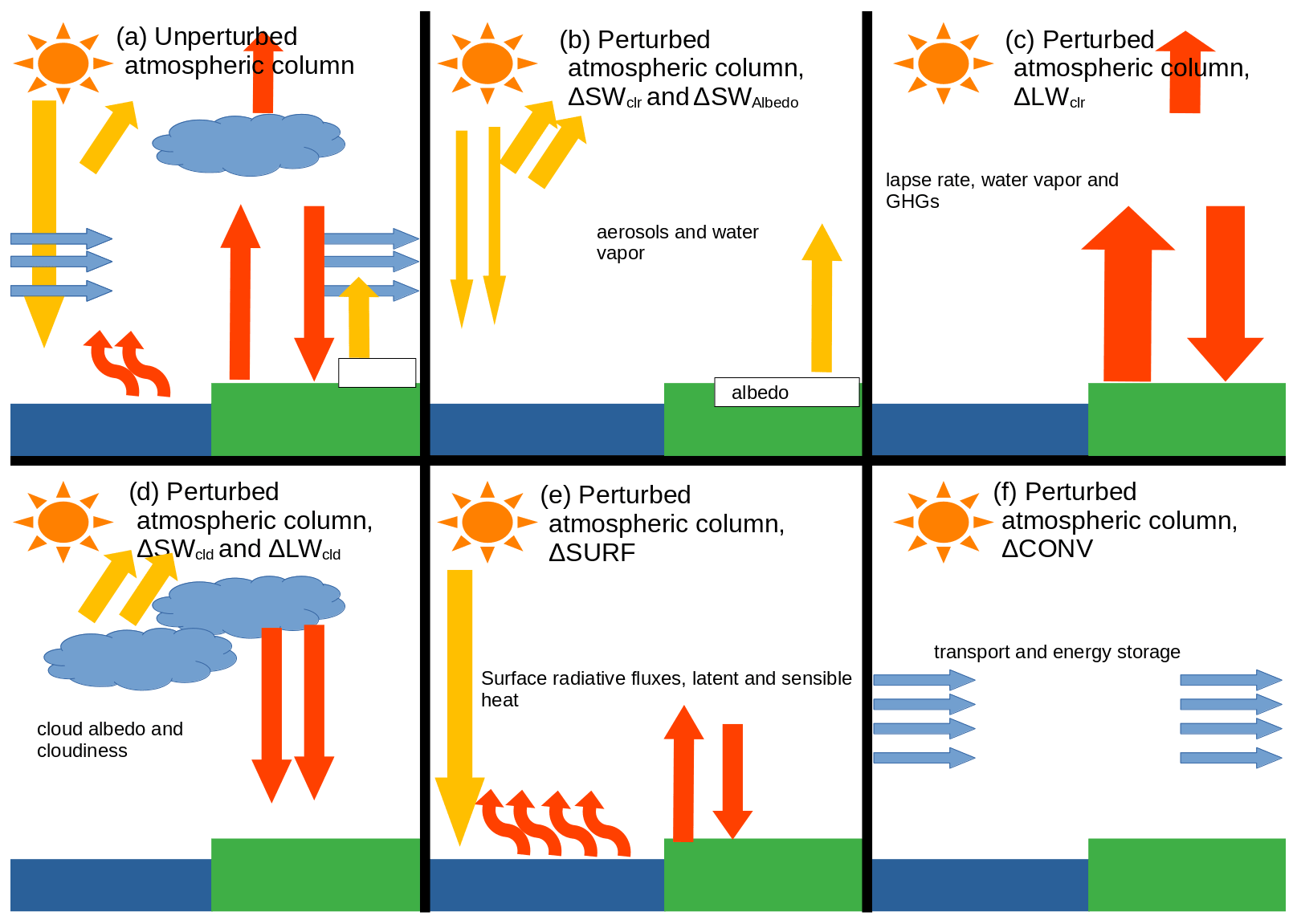
Figure 1 Illustration of the local atmospheric energy budget in a single atmospheric column from the surface to the top of model atmosphere (TOA). We attribute the change in local surface temperature to changes in different terms of the local energy budget. (a) Unperturbed conditions, where red arrows indicate longwave (thermal) radiation, yellow arrows indicate shortwave (solar) radiation, blue arrows indicate horizontal incoming and outgoing energy, and curvy red arrows indicate latent and sensible heat. Under perturbed conditions, we decompose the change in the energy budget to (b) the change in TOA solar radiation due to changes in surface albedo and to the change in shortwave clear-sky flux (separately). The change in shortwave clear-sky flux is mainly caused by changes in aerosol concentrations or changes in atmospheric water vapor; (c) the change in longwave TOA flux, which is mainly caused by changes in atmospheric water vapor concentrations, atmospheric thermal structure (lapse rate) or greenhouse gas concentrations; (d) changes in longwave and shortwave TOA fluxes, separately, due to changes in cloudiness and cloud microphysics; (e) the combined change in surface energy balance, including the change in the net shortwave and longwave energy flux into the surface and changes in latent and sensible heat fluxes; (f) the combined change in horizontal energy transport and internal energy of the atmospheric column, calculated from the convergence of energy.

2 Materials and methods

2.1 Decomposition of the surface temperature response

We attribute local surface air temperature response to different net energetic components, namely, to changes in local longwave fluxes associated with changes in clear-sky and cloud emissivity ($\mathrm{\Delta }{\mathrm{LW}}_{\mathrm{TOA},\mathrm{clr},\mathit{\epsilon }}^{\uparrow }$ and $\mathrm{\Delta }{\mathrm{LW}}_{\mathrm{TOA},\mathrm{cld},\mathit{\epsilon }}^{\uparrow }$, respectively, with the arrow indicating the vector direction towards space) at TOA, changes in shortwave fluxes due to changes in clear-sky absorption and reflection as well as changes in cloudiness and cloud radiative properties ($\mathrm{\Delta }{\mathrm{SW}}_{\mathrm{TOA},\mathrm{clr},\mathit{\epsilon }}^{\downarrow }$, and $\mathrm{\Delta }{\mathrm{SW}}_{\mathrm{TOA},\mathrm{cld}}^{\downarrow }$), changes in surface energy fluxes ($\mathrm{\Delta }{F}_{\mathrm{SURF}}^{\downarrow }$, essentially representing changes in atmosphere-to-ocean net heat flux), and convergence of atmospheric energy (ΔCONV, representing horizontal atmospheric heat transport). These changes are illustrated in Fig. 1. We use the method presented in Räisänen and Ylhäisi (2015), Räisänen (2017), and Merikanto et al. (2021). The method is based on a concept of planetary emissivity (Cess, 1976), which links the local surface air temperature (T) to the outgoing longwave radiation at the top of the atmospheric column (${\mathrm{LW}}_{\mathrm{TOA}}^{\uparrow }$),

$$\begin{array}{}\text{(1)}& {\mathit{\epsilon }}_{\mathrm{eff}}={\displaystyle \frac{{\mathrm{LW}}_{\mathrm{TOA}}^{\uparrow }}{\mathit{\sigma }{T}^{\mathrm{4}}}},\end{array}$$

where ε_eff is an effective local planetary emissivity, and σ is the Boltzmann constant. Then, letting [ ] mark the mean state between baseline and perturbed climates, the change in outgoing longwave radiation between the two climate states can be written as

$$\begin{array}{}\text{(2)}& \begin{array}{rl}\mathrm{\Delta }{\mathrm{LW}}_{\mathrm{TOA}}^{\uparrow }& =\mathrm{4}\mathit{\sigma }\left[{\mathit{\epsilon }}_{\mathrm{eff}}\right]\left[T^{\mathrm{3}}\right]\mathrm{\Delta }T+\mathit{\sigma }\mathrm{\Delta }{\mathit{\epsilon }}_{\mathrm{eff}}\left[T^{\mathrm{4}}\right]\\ & =D\mathrm{\Delta }T+\mathrm{\Delta }{\mathrm{LW}}_{\mathrm{TOA},\mathit{\epsilon }}^{\uparrow },\end{array}\end{array}$$

where DΔT is the local change in outgoing thermal radiation at constant emissivity (i.e at fixed thermal atmospheric structure and water vapor concentration); hence, D represents the local Planck feedback parameter. $\mathrm{\Delta }{\mathrm{LW}}_{\mathrm{TOA},\mathit{\epsilon }}^{\uparrow }$ is the local change in the outgoing thermal radiation associated with the change in the local planetary emissivity.

The rate of energy change within an atmospheric column is given by the energy balance equation:

$$\begin{array}{}\text{(3)}& {\displaystyle \frac{\mathit{\delta }E}{\mathit{\delta }t}}={\mathrm{SW}}_{\mathrm{TOA}}^{\downarrow }-{\mathrm{LW}}_{\mathrm{TOA}}^{\uparrow }-F_{\mathrm{SURF}}^{\downarrow }+C^{\leftarrow },\end{array}$$

where $\frac{\mathit{\delta }E}{\mathit{\delta }t}$ is the change in internal energy within the column with respect to time, ${\mathrm{SW}}_{\mathrm{TOA}}^{\downarrow }$ is the net incoming flux of solar radiation, and C^← is the horizontal transport of energy to the column; the net downward heat flux $F_{\mathrm{SURF}}^{\downarrow }$ into the surface is given by

$$\begin{array}{}\text{(4)}& F_{\mathrm{SURF}}^{\downarrow }={\mathrm{SW}}_{\mathrm{SURF}}^{\downarrow }+{\mathrm{LW}}_{\mathrm{SURF}}^{\downarrow }-{\mathrm{SH}}^{\uparrow }-{\mathrm{LH}}^{\uparrow }.\end{array}$$

The change in ${\mathrm{LW}}_{\mathrm{TOA}}^{\uparrow }$ between two climate states can thus be written as

$$\begin{array}{}\text{(5)}& \mathrm{\Delta }{\mathrm{LW}}_{\mathrm{TOA}}^{\uparrow }=\mathrm{\Delta }{\mathrm{SW}}_{\mathrm{TOA}}^{\downarrow }-\mathrm{\Delta }{F}_{\mathrm{SURF}}^{\downarrow }+\mathrm{\Delta }\left(C^{\leftarrow }-{\displaystyle \frac{\mathit{\delta }E}{\mathit{\delta }t}}\right).\end{array}$$

Using Eq. (2) with Eq. (5), the local change in surface temperature can be decomposed to different energetic components as

$$\begin{array}{}\text{(6)}& \begin{array}{rl}\mathrm{\Delta }T& =-{\displaystyle \frac{\mathrm{\Delta }{\mathrm{LW}}_{\mathrm{TOA},\mathit{\epsilon }}^{\uparrow }}{D}}+{\displaystyle \frac{\mathrm{\Delta }{\mathrm{SW}}_{\mathrm{TOA}}^{\downarrow }}{D}}-{\displaystyle \frac{\mathrm{\Delta }{F}_{\mathrm{SURF}}^{\downarrow }}{D}}\\ & +{\displaystyle \frac{\mathrm{\Delta }\left(C^{\leftarrow }-\frac{\mathit{\delta }E}{\mathit{\delta }t}\right)}{D}}=\mathrm{\Delta }{T}_{\mathrm{LW}}+\mathrm{\Delta }{T}_{\mathrm{SW}}\\ & +\mathrm{\Delta }{T}_{\mathrm{SURF}}+\mathrm{\Delta }{T}_{\mathbf{CONV}}.\end{array}\end{array}$$

ΔT_LW, ΔT_SW, and ΔT_SURF can be calculated directly from the standard energy flux output of the models, with ΔT_CONV as a residual term. ΔT_CONV includes both horizontal energy transport and change in local atmospheric energy storage which is insignificant at annual timescales. Furthermore, ΔT_SW can be decomposed into clear-sky, cloud, albedo, and nonlinear terms using the Approximate Partial Radiative Perturbation (APRP) method (Taylor et al., 2007),

$$\begin{array}{}\text{(7)}& \begin{array}{rl}\mathrm{\Delta }{\mathrm{SW}}_{\mathrm{TOA}}^{\downarrow }& =\mathrm{\Delta }{\mathrm{SW}}_{\mathrm{TOA},\mathrm{in}}^{\downarrow }+\mathrm{\Delta }{\mathrm{SW}}_{\mathrm{TOA},\mathrm{clr}}^{\downarrow }+\mathrm{\Delta }{\mathrm{SW}}_{\mathrm{TOA},\mathrm{cld}}^{\downarrow }\\ & +\mathrm{\Delta }{\mathrm{SW}}_{\mathrm{TOA},\mathrm{Albedo}}^{\downarrow }+\mathrm{\Delta }{\mathrm{SW}}_{\mathrm{TOA},\mathrm{nl}}^{\downarrow },\end{array}\end{array}$$

where $\mathrm{\Delta }{\mathrm{SW}}_{\mathrm{TOA},\mathrm{in}}^{\downarrow }$ is the change in incoming solar radiation, $\mathrm{\Delta }{\mathrm{SW}}_{\mathrm{TOA},\mathrm{clr}}^{\downarrow }$ is the change in net TOA solar radiation due to changes in clear-sky radiative properties of the atmosphere, $\mathrm{\Delta }{\mathrm{SW}}_{\mathrm{TOA},\mathrm{cld}}^{\downarrow }$ the change in net TOA solar radiation due to changes in clouds, $\mathrm{\Delta }{\mathrm{SW}}_{\mathrm{TOA},\mathrm{Albedo}}^{\downarrow }$ the change in net TOA solar radiation due to change in surface albedo, and $\mathrm{\Delta }{\mathrm{SW}}_{\mathrm{TOA},\mathrm{nl}}^{\downarrow }$ is a nonlinear correction term arising from the APRP method. $\mathrm{\Delta }{\mathrm{SW}}_{\mathrm{TOA},\mathrm{in}}^{\downarrow }$ is constant if the incoming solar flux is constant. $\mathrm{\Delta }{\mathrm{SW}}_{\mathrm{TOA},\mathrm{nl}}^{\downarrow }$ is typically negligibly small and can be ignored (Räisänen, 2017; Merikanto et al., 2021).

Also $\mathrm{\Delta }{\mathrm{LW}}_{\mathrm{TOA},\mathit{\epsilon }}^{\uparrow }$ can be decomposed into clear-sky (CS) and cloud radiative effect (CRE) components:

$$\begin{array}{}\text{(8)}& \mathrm{\Delta }{\mathrm{LW}}_{\mathrm{TOA},\mathit{\epsilon }}^{\uparrow }=\mathrm{\Delta }{\mathrm{LW}}_{\mathrm{TOA},\mathrm{CS},\mathit{\epsilon }}^{\uparrow }+\mathrm{\Delta }{\mathrm{LW}}_{\mathrm{TOA},\mathrm{CRE},\mathit{\epsilon }}^{\uparrow }.\end{array}$$

First the left-hand side in Eq. (8) is obtained by substituting the all-sky LW flux to Eq. (2). Second, the first (clear-sky) right-hand side term in Eq. (8) is obtained by substituting the clear-sky flux into Eq. (2). The CRE component is obtained as a residual. However, $\mathrm{\Delta }{\mathrm{LW}}_{\mathrm{TOA},\mathrm{CRE},\mathit{\epsilon }}^{\uparrow }$ is affected by changes in noncloud feedbacks (water vapor and air temperature), making it a negatively biased approximation of the actual cloud longwave feedback. To obtain a more accurate estimation of the actual cloud contribution to longwave emissivity change, we applied the radiative kernel method of Soden et al. (2008). With this method, a correction factor can be calculated:

$$\begin{array}{}\text{(9)}& \begin{array}{rl}\mathrm{\Delta }{\mathrm{LW}}_{\mathrm{corr}}^{\uparrow }& =\left(K_T-K_T^{\mathrm{clr}}\right)\mathrm{\Delta }T+{\sum }_i\left(K_{T_i}-K_{T_i}^{\mathrm{clr}}\right)\mathrm{\Delta }{T}_i\\ & +{\sum }_i\left(K_{{\mathrm{w}}_i}-K_{{\mathrm{w}}_i}^{\mathrm{clr}}\right)\mathrm{\Delta }{\left(\ln q\right)}_i,\end{array}\end{array}$$

where K_T, $K_{T_i}$, and $K_{{\mathrm{w}}_i}$ represent radiative kernels where each state variable (surface temperature, temperature profile and water vapor respectively) is perturbed by unit change. The corrected clear-sky and cloud longwave emissivity changes then become

$$\begin{array}{}\text{(10a)}& {\displaystyle }\mathrm{\Delta }{\mathrm{LW}}_{\mathrm{TOA},\mathrm{clr},\mathit{\epsilon }}^{\uparrow }=\mathrm{\Delta }{\mathrm{LW}}_{\mathrm{TOA},\mathrm{CS},\mathit{\epsilon }}^{\uparrow }+\mathrm{\Delta }{\mathrm{LW}}_{\mathrm{corr}}^{\uparrow },\text{(10b)}& {\displaystyle }\mathrm{\Delta }{\mathrm{LW}}_{\mathrm{TOA},\mathrm{cld},\mathit{\epsilon }}^{\uparrow }=\mathrm{\Delta }{\mathrm{LW}}_{\mathrm{TOA},\mathrm{CRE},\mathit{\epsilon }}^{\uparrow }-\mathrm{\Delta }{\mathrm{LW}}_{\mathrm{corr}}^{\uparrow }.\end{array}$$

All results have been calculated using three different kernels, ECHAM (Block and Mauritsen, 2013), GFDL (Pendergrass et al., 2018), and HadGEM2 (Smith, 2018), to obtain a better estimate of the overall cloud effect. The correction factor of Eq. (9) has been calculated as an average of the three kernels.

Finally, the local surface temperature responses are decomposed as

$$\begin{array}{}\text{(11)}& \begin{array}{rl}\mathrm{\Delta }T& =-{\displaystyle \frac{\mathrm{\Delta }{\mathrm{LW}}_{\mathrm{TOA},\mathrm{clr},\mathit{\epsilon }}^{\uparrow }}{D}}-{\displaystyle \frac{\mathrm{\Delta }{\mathrm{LW}}_{\mathrm{TOA},\mathrm{cld},\mathit{\epsilon }}^{\uparrow }}{D}}\\ & +{\displaystyle \frac{\mathrm{\Delta }{\mathrm{SW}}_{\mathrm{TOA},\mathrm{clr}}^{\downarrow }}{D}}+{\displaystyle \frac{\mathrm{\Delta }{\mathrm{SW}}_{\mathrm{TOA},\mathrm{cld}}^{\downarrow }}{D}}\\ & +{\displaystyle \frac{\mathrm{\Delta }{\mathrm{SW}}_{\mathrm{TOA},\mathrm{Albedo}}^{\downarrow }}{D}}-{\displaystyle \frac{\mathrm{\Delta }{F}_{\mathrm{SURF}}^{\downarrow }}{D}}+{\displaystyle \frac{\mathrm{\Delta }\left(C^{\to }-\frac{\mathit{\delta }E}{\mathit{\delta }t}\right)}{D}}\\ & =-\mathrm{\Delta }{\mathrm{LW}}_{\mathrm{clr},\mathit{\epsilon }}-\mathrm{\Delta }{\mathrm{LW}}_{\mathrm{cld},\mathit{\epsilon }}+\mathrm{\Delta }{\mathrm{SW}}_{\mathrm{clr}}+\mathrm{\Delta }{\mathrm{SW}}_{\mathrm{cld}}\\ & +\mathrm{\Delta }{\mathrm{SW}}_{\mathrm{Albedo}}+\mathrm{\Delta }\mathrm{SURF}+\mathrm{\Delta }\mathrm{CONV}.\end{array}\end{array}$$

In the above equation, the temperature responses related to the first five components build up from a sum of the instant radiative forcing (if any), rapid adjustments associated with the component, and a temperature-dependent feedback which adjusts its magnitude as the surface temperature changes, normalized by D (the Planck feedback). Therefore, temperature responses related to these terms are functions of a constant term (forcing and adjustments) and a time-dependent term (the impact of feedback due to surface temperature changes). For example, the LW flux response to a change in clear-sky longwave emissivity is $\mathrm{\Delta }{\mathrm{LW}}_{\mathrm{TOA},\mathrm{clr},\mathit{\epsilon }}^{\uparrow }\approx F_{\mathrm{TOA},\mathrm{LW},\mathrm{clr},\mathit{\epsilon }}^{\uparrow }-{\mathit{\lambda }}_{\mathrm{LR}+\mathrm{LWWV}}\mathrm{\Delta }T$ in a linearized forcing-feedback framework, where $F_{\mathrm{TOA},\mathrm{LW},\mathrm{clr}}^{\uparrow }$ is the longwave component of the effective radiative forcing, and λ_LR+LWWV is the combined longwave lapse-rate and water vapor feedback (e.g., Crook and Forster, 2011). Similarly, $\mathrm{\Delta }{\mathrm{LW}}_{\mathrm{TOA},\mathrm{cld},\mathit{\epsilon }}^{\uparrow }\approx F_{\mathrm{TOA},\mathrm{LW},\mathrm{cld},\mathit{\epsilon }}^{\uparrow }-{\mathit{\lambda }}_{\mathrm{LW}\mathrm{\_}\mathrm{cld}}\mathrm{\Delta }T$, $\mathrm{\Delta }{\mathrm{SW}}_{\mathrm{TOA},\mathrm{clr}}^{\downarrow }\approx F_{\mathrm{TOA},\mathrm{SW},\mathrm{clr}}^{\downarrow }+{\mathit{\lambda }}_{\mathrm{SWWV}}\mathrm{\Delta }T$, $\mathrm{\Delta }{\mathrm{SW}}_{\mathrm{TOA},\mathrm{cld}}^{\downarrow }\approx F_{\mathrm{TOA},\mathrm{SW},\mathrm{cld}}^{\downarrow }+{\mathit{\lambda }}_{\mathrm{SW},\mathrm{cld}}\mathrm{\Delta }T$, and $\mathrm{\Delta }{\mathrm{SW}}_{\mathrm{TOA},\mathrm{Albedo}}^{\downarrow }\approx F_{\mathrm{TOA},\mathrm{SW},\mathrm{Albedo}}^{\downarrow }+{\mathit{\lambda }}_{\mathrm{SW},\mathrm{Albedo}}\mathrm{\Delta }T$; $\mathrm{\Delta }{F}_{\mathrm{SURF}}^{\downarrow }$ and $\mathrm{\Delta }\left(C^{\to }-\frac{\mathit{\delta }E}{\mathit{\delta }t}\right)$ do not have direct counterparts in the linear forcing-feedback analysis, and they have been incorporated as part of the energy budget in regional forcing-feedback analysis in various ways in the literature (Crook et al., 2011; Feldl and Roe, 2013; Lu and Cai, 2009). In the last line of Eq. (11), the terms without TOA suffix, i.e., the radiative components divided by D, are in units of temperature. Hereafter, we will use these terms as shorthand notations when discussing the various temperature responses in the text.

2.2 Decomposition of the standard deviation in surface temperature response

Decomposing the temperature responses ΔT_i also allows us to decompose their contributions CSD_i to the model-to-model standard deviations σ_ΔT of the total temperature responses by,

$$\begin{array}{}\text{(12)}& {\mathrm{CSD}}_i={\displaystyle \frac{\mathrm{cov}\left(\mathrm{\Delta }{T}_i,\mathrm{\Delta }T\right)}{{\mathit{\sigma }}_{\mathrm{\Delta }T}}}=r_i{\mathit{\sigma }}_{\mathrm{\Delta }{T}_i},\end{array}$$

where cov(ΔT_iΔT) is the model-to-model covariance between the ith time-averaged local temperature response component and the total local temperature response of a model experiment, where r_i and ${\mathit{\sigma }}_{\mathrm{\Delta }{T}_i}$ are their model-to-model correlation and the standard deviation, respectively, and σ_ΔT is the standard deviation of time-averaged temperature responses in different models. CSD_i values sum up to the intermodel standard deviations of the temperature responses,

$$\begin{array}{}\text{(13)}& {\sum }_i{\mathrm{CSD}}_i={\mathit{\sigma }}_{\mathrm{\Delta }T}.\end{array}$$

2.3 Models and simulations

We use climate model data from (PDRMIP) (Myhre et al., 2017). In PDRMIP, several independent climate models were used to simulate various idealized climate perturbations. The models used in this study are listed in Table 1. According to Knutti (2013), all these models belong to different model families and hence are largely independent of each other. Our study uses data from experiments of instant doubling of CO₂ concentrations (co2x2), tripling of CH₄ concentrations (ch4x3), 5-fold increasing sulfate emission (sulx5), and 10-fold increasing black carbon emissions (bcx10) (see Table 2). Perturbations were relative to the baseline which had the present-day (models except HadGEM2-ES) or the preindustrial (HadGEM2-ES) levels of anthropogenic forcing agents.

Table 1 PDRMIP models used in this study, ocean and aerosol configuration of the model, and which aerosol–cloud interactions are included.

Table 2 Description of PDRMIP experiments.

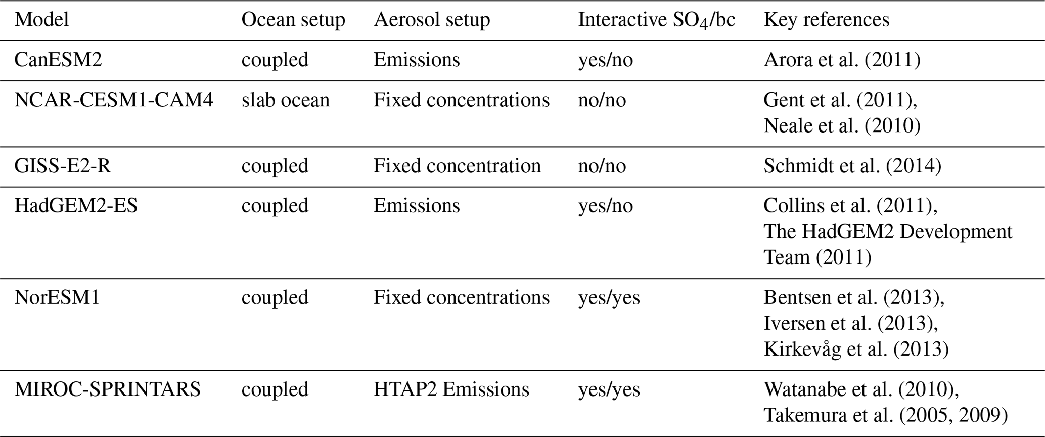
All simulations consisted of 100-year baseline and perturbed runs, and the last 50 years of these runs are used for the temperature response analysis carried out here. The PDRMIP experiments also included additional fixed sea surface temperature runs, which we use for the calculation of the effective radiative forcing (ERF_fsst) associated with each climate perturbation. We also calculated the effective radiative forcing by regressing the top-of-atmosphere radiative imbalance against surface temperature change (ERF_bcx10reg) by using the full 100-year time series of experiments, as further discussed below. Aerosol emissions were either defined explicitly or by multiplying predefined concentrations derived from AeroCom Phase II (Myhre et al., 2013) (see Table 1). Only NorESM1 and MIROC-SPRINTARS include the aerosol indirect effect (the Twomey effect) for black carbon; however, the meteorological adjustments (the semidirect effect) are inherent in all models. The aerosol cloud effects from sulfate are included in all models except NCAR-ESM1-CAM4 and GISS-E2-R. We include the six PDRMIP models which had reported all necessary fields for this analysis.

2.4 Global TOA radiative forcing and surface temperature responses of analyzed experiments

In this paper, we focus on decomposed local and global temperature responses normalized by the global effective radiative forcing (ERF_fsst) obtained from fixed-sea-surface-temperature experiments for each modeled perturbation. The normalization by ERF_fsst enables us to compare the temperature responses of different modeled perturbations with each other on a level ground, as ERF_fsst varies in sign and magnitude between different perturbations. Also, particularly in aerosol and methane experiments, the modeled ERF_fsst values vary between different models, likely due to differences in model aerosol setups and baseline methane concentrations.

Figure 2 shows the calculated effective radiative forcings and the global mean temperature responses (the difference in perturbed climate for the years 50–100 and the corresponding years from the base case) in the analyzed PDRMIP experiments. The effective radiative forcing is calculated from both fixed-sea-surface-temperature simulations (ERF_fsst, no land-warming corrections included) and by regressing the top-of-atmosphere radiative imbalance with respect to surface temperature change by using the full 100-year time series of experiments (ERF_reg; Gregory et al., 2004).

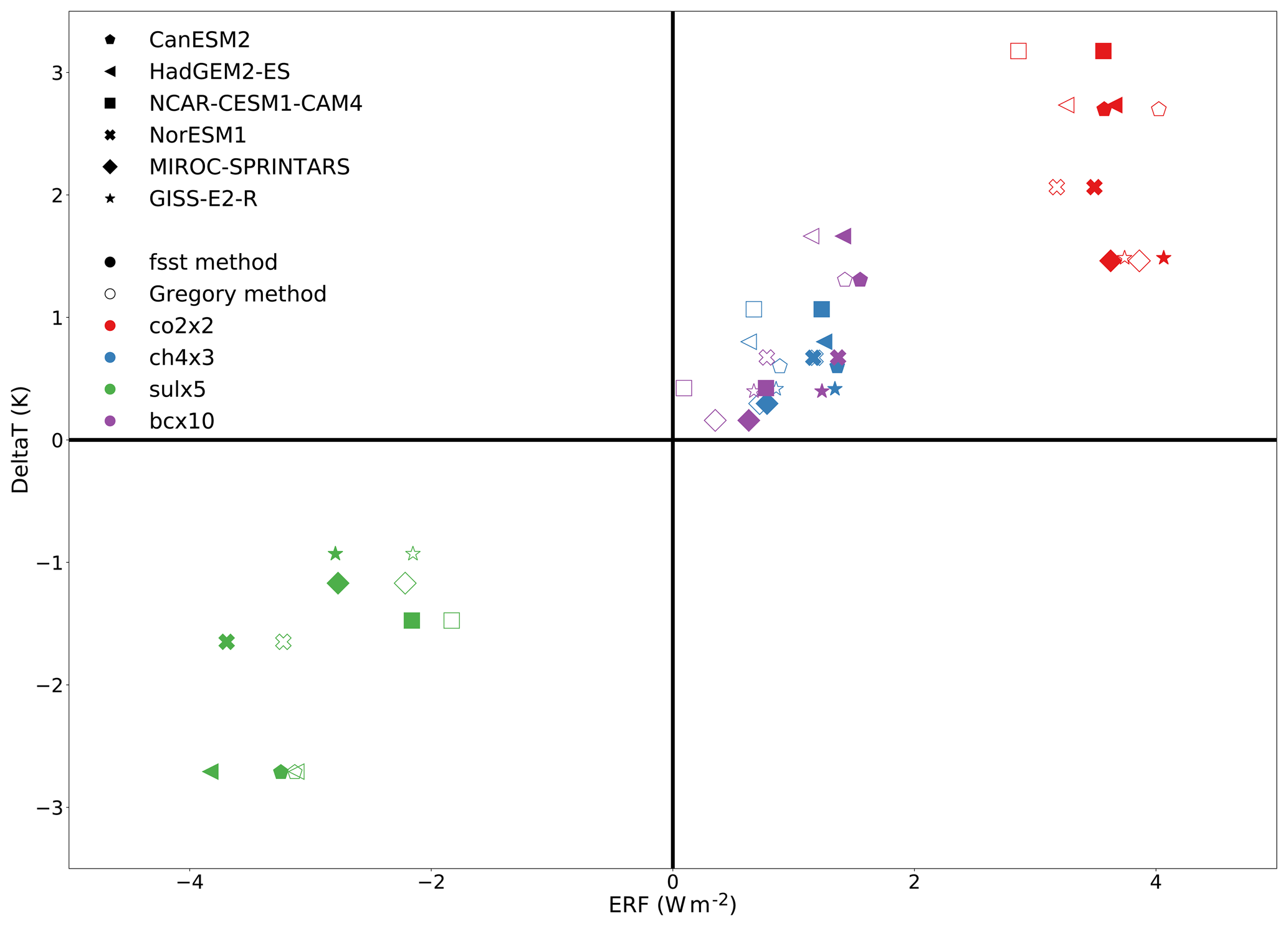
Figure 2 The global average temperature responses for each experiment and each model (y axis) averaged over years 50–100 after the sudden introduction of climate perturbations. The calculated ERFs for each experiment and model are shown on the x axis, with non-filled marks indicating the ERF_reg obtained using the Gregory method and the filled markers indicating ERF_fsst obtained from fixed-sea-surface-temperature simulations.

One of the models (NCAR-CESM1-CAM) was ran using a slab ocean configuration, while the rest of the models contained fully interactive ocean configurations. Since the equilibrium is reached in a few decades with slab ocean configurations but for the fully interactive ocean configuration it takes centuries, the perturbed experiments with models besides NCAR-CESM1-CAM are still in a transient state. As a multimodel mean over the years 50–100 of the perturbed runs, the doubling of CO₂ concentration (red marks) leads to a 2.27 K (± 0.65 K) rise in global surface temperatures, with a model-to-model standard deviation (SD) of 0.65 K. The corresponding values are for tripling of CH₄ (blue marks) 0.64 K (± 0.25 K), 5-fold increasing sulfate aerosols (green marks) −1.77 K (± 0.70 K), and 10-fold increasing black carbon (purple) aerosols 0.77 K (± 0.54 K). The exact numbers for each forcer and model are shown in the Supplement (Tables S1–S4), and the estimated equilibrium temperature responses for each of the experiments is shown in Table S5.

The multimodel-mean ERF_fsst values for co2x2, ch4x3, sulx5, and bcx10 experiments are, respectively, 3.66 W m⁻² (SD 0.19 W m⁻²), 1.19 W m⁻² (SD 0.19 W m⁻²), −3.08 W m⁻² (SD 0.58 W m⁻²), and 1.16 W m⁻² (SD 0.34 W m⁻²). When the effective forcings are calculated from regressions using the full 100-year time series, the corresponding ERF_reg values are 3.49 W m⁻², (SD 0.41 W m⁻²), 0.82 W m⁻² (SD 0.19 W m⁻²), −2.61 W m⁻² (SD 0.56 W m⁻²), and 0.74 W m⁻² (SD 0.45 W m⁻²). Tang (2019) has carried out complete analysis of ERF_fsst and ERF_reg for the PDRMIP data, and our values are consistent with the values presented there. We also refer the reader to Tang (2019) for the ERF_fsst values obtained with the land warming correction accounted for and for ERF_reg calculated from the first 30 years of perturbed experiments.

Figure 2 shows that only a weak relationship between the model-to-model values in ERF_fsst (or ERF_reg) and the model-to-model spread in temperature response can be seen for co2x2 and ch4x3 experiments, while some relationship exists for the sulx5 and bcx10 experiments. Correlations between the models' temperature response and their ERF_fsst values for co2x2 and ch4x3 are −0.52 and 0.43, while with sulx5 and bcx10 correlations are 0.61 and 0.78, respectively. As also visible in Fig. 1 for individual models, the application of the regression method for the full 100-year time series of experiments provides consistently lower values for ERF compared to values obtained from fixed sea surface temperature calculations. Overall, ERF_fsst appears to be a more suitable choice for the surface temperature response normalization of different experiments due to very small values of ERF_reg associated with some bcx10 experiments. Tang et al. (2019) also calculated ERF values that account for land warming adjustment, which leads to significantly larger ERF estimation than using fixed sea surface simulations. However, this does not improve the correlation between temperature and ERF (see Fig. S5).

3 Results

In the following sections, we present decomposed effective temperature responses for each analyzed experiment and model-to-model spread of these decompositions. The effective surface temperature responses and their decompositions are calculated for each atmospheric column separately from the average differences in perturbed climates for the years 50–100 after a sudden perturbation and the corresponding years from the baseline simulations without perturbations. The local temperature responses are normalized by the globally averaged ERF_fsst for each experiment (hence the term effective). Scaling with ERF_fsst allows for a simpler comparison of responses between different forcing agents, but it also changes the sign of responses in the case of sulx5 experiments. This is because, in contrast to the other three forcing agents, the radiative forcing is negative for increasing sulfate concentrations.

The local temperature responses related to longwave and shortwave TOA components build up from a combination of the local instantaneous top-of-atmosphere radiative forcing and rapid adjustments associated with each term, as well as a temperature-dependent feedback which adjusts its magnitude as the surface temperature changes, as described in the end of Sect. 2.1. Therefore, temperature responses related to these components are functions of a forcing (if any), rapid adjustments, and a time-dependent term (the impact of feedback as surface temperature changes).

The temperature response decomposition applied here relies on a local conservation of energy in each atmospheric column; hence, the sums of individual temperature response components generate the local total surface temperature responses with high accuracy. Below, Sect. 3.1 presents the globally averaged results. Section 3.2 then presents the regional distributions of the decomposed surface temperature responses and their zonal averages. Section 3.3 presents the regional and latitudinal distributions of the model-to-model standard deviations of the effective temperature components and the contributions of each of the decomposed surface temperature response components to the total standard deviations of the responses.

3.1 Decomposed global effective surface temperature responses for different forcers

Figure 3 shows the globally averaged effective surface temperature responses and their decomposed components for each model and perturbation experiment, calculated by using the temperature decomposition method described in Sect. 2.1. The components of the effective surface temperature responses describe the combined global contributions of the TOA forcing (in the case of clear-sky ΔLW_clr and ΔSW_clr components and ΔLW_cld and ΔSW_cld cloud components) and the effects of rapid adjustments and feedbacks associated with each component. Of the components not associated with the TOA radiative forcing, ΔSW_Albedo is directly related to the response due to surface albedo feedback, ΔSURF is a measure of the surface energy flux imbalance on global surface temperatures due to oceanic heat uptake in the models, and ΔCONV describes the impact of horizontal surface energy transport and change in atmospheric heat uptake. The models which have a fully coupled ocean have not fully reached equilibrium; therefore, there is still some heat flux from the atmosphere to the ocean. Thus, the effective temperature response from this heat flux is always negative. Globally, ΔCONV averages effectively to zero in each experiment since the energy transport only redistributes regional surface temperature effects, and the change in atmospheric heat uptake is negligible on annual or longer timescales (Räisänen, 2017).

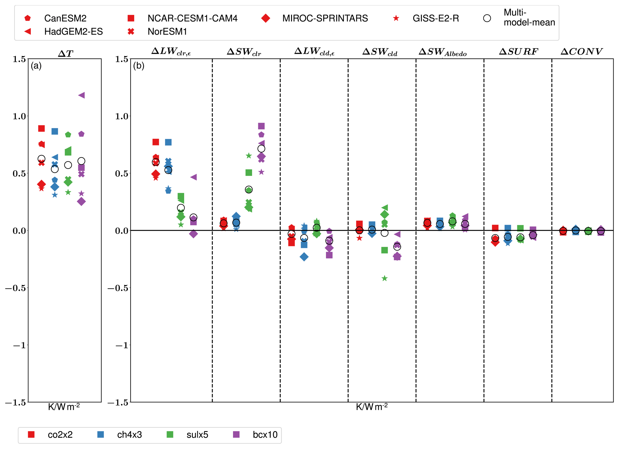
Figure 3 The global mean effective temperature response and its decomposition, calculated as the difference between means over the last 50 years of the perturbed and the baseline experiments. (a) The effective temperature response (absolute temperature response divided by ERF_fsst) for the six models shown with different symbols and four different radiative forcers shown with different colors. (b) The decomposition of the effective temperature response to different energetic components. Individual panels in (b) describe (from the left) the contributions to total effective temperature response due to the change in longwave clear-sky emissivity (ΔLW_clr,ε), change in TOA shortwave radiation (ΔSW_clr), change in longwave cloud emissivity (ΔLW_cld,ε), net ocean surface heat flux (ΔSURF), and change in atmospheric energy transport (ΔCONV).

The total effective temperature responses (temperature response divided by the ERF_sst) for co2x2, ch4x3, sulx5, and bcx10 experiments are 0.63 K W⁻¹ m² (SD 0.19), 0.54 K W⁻¹ m² (SD 0.18), 0.57 K W⁻¹ m² (SD 0.18) and 0.61 K W⁻¹ m² (SD 0.32), respectively. Hence, the mean value and the model-to-model spread in total effective temperature response is similar for different forcers, as shown in previous PDRMIP studies (Richardson et al., 2018; Samset et al., 2018; Stjern et al., 2017). The change in TOA longwave clear-sky emissivity is the key driver of the effective temperature response for the greenhouse gas experiments (co2x2 and ch4x3), with the multimodel-mean effective surface temperature responses to ΔLW_clr matching nearly exactly the overall responses (0.60 K W⁻¹ m² ± 0.10 and 0.53 K W⁻¹ m² ± 0.18, respectively). ΔLW_clr results from the change in clear-sky planetary emissivity, i.e., from the combination of the longwave clear-sky radiative forcing and its adjustments, and the change in the thermal structure of the atmosphere and water vapor concentrations which evolve with the surface temperature response (lapse rate and water vapor feedbacks). The large model-to-model spread compared to other terms is discussed more in Sect. 3.3. In Sect. 4 we discuss why our model-to-model spread differs from example values presented by Zelinkta et al. (2020). For the aerosol experiments (sulx5 and bcx10), the effective temperature response associated with ΔLW_clr is only a small contribution to the total temperature response. This is because for aerosols the instantaneous radiative forcing associated with the longwave clear-sky radiation is small.

The differences in effective temperature responses associated with ΔSW_clr between the greenhouse gas and aerosol forcers can be understood via a similar narrative as in the case of ΔLW_clr responses. The total effective temperature response for aerosol experiments (sulx5 and bcx10) is largely dominated by the temperature response to ΔSW_clr, since much of the instantaneous aerosol radiative forcing takes place via this channel. For the greenhouse gas experiments, the temperature response to ΔSW_clr originates from the shortwave water vapor feedback and direct greenhouse gas's shortwave forcing (Etminan et al., 2016), and its model-mean contribution to total effective temperature response is comparable to that from the albedo response (∼ 10 %).

The multimodel-mean effective temperature responses related to ΔLW_cld and ΔSW_cld are close to zero for all experiments besides bcx10, for which the cloud temperature responses modestly oppose the total effective temperature response. With bcx10, the net cloud effect is cooling across different latitudes, despite variations between ΔLW_cld and ΔSW_cld. The increase of low-level clouds over the Arctic regions and reductions of clouds in upper troposphere (see Fig. S4) due to BC forcing are typical cloud responses, and these dominate the rapid adjustments and lead to dampening of the surface response (Stjern et al., 2017). For the sulx5 experiment, the model-mean ΔSW_cld is near zero, and its spread is high between the models. A significant part of the spread is related to the lack of cloud–aerosol interaction in NCAR-CESM1-CAM4 and GISS-E2-R. In these models, ΔSWcld reduces the sulfate-induced global mean cooling, whereas it amplifies the cooling in the other models.

The global effective temperature response from the changes in surface albedo is similar across each experiment. The mean effective temperature response due to albedo change varies from ∼ 10 % (co2x2, chx3 and bcx10) to 14 % (sulx5) of the total effective temperature response. In the aerosol experiments the aerosol setup has a significant effect on the temperature contribution of the surface albedo change. Emission-driven models tend to produce a higher albedo effective temperature response than the concentration-driven models.

3.2 Origins of regional temperature responses for different climate forcers

The model-mean spatial distributions of effective temperature responses and their decomposed components are shown in Fig. 4. The zonal means of different components are shown in Fig. 5, where we have summed up the contributions of surface and atmospheric energy transport components (ΔSURF and ΔCONV) due to their strong tendency to balance each other regionally. Furthermore, the total response due to clouds (ΔLW_cld and ΔSW_cld) is shown in Fig. 5 together with individual cloud components. Again, we remind the reader that scaling all results with ERF_fsst changes the sign of responses in the sulx5 experiments.

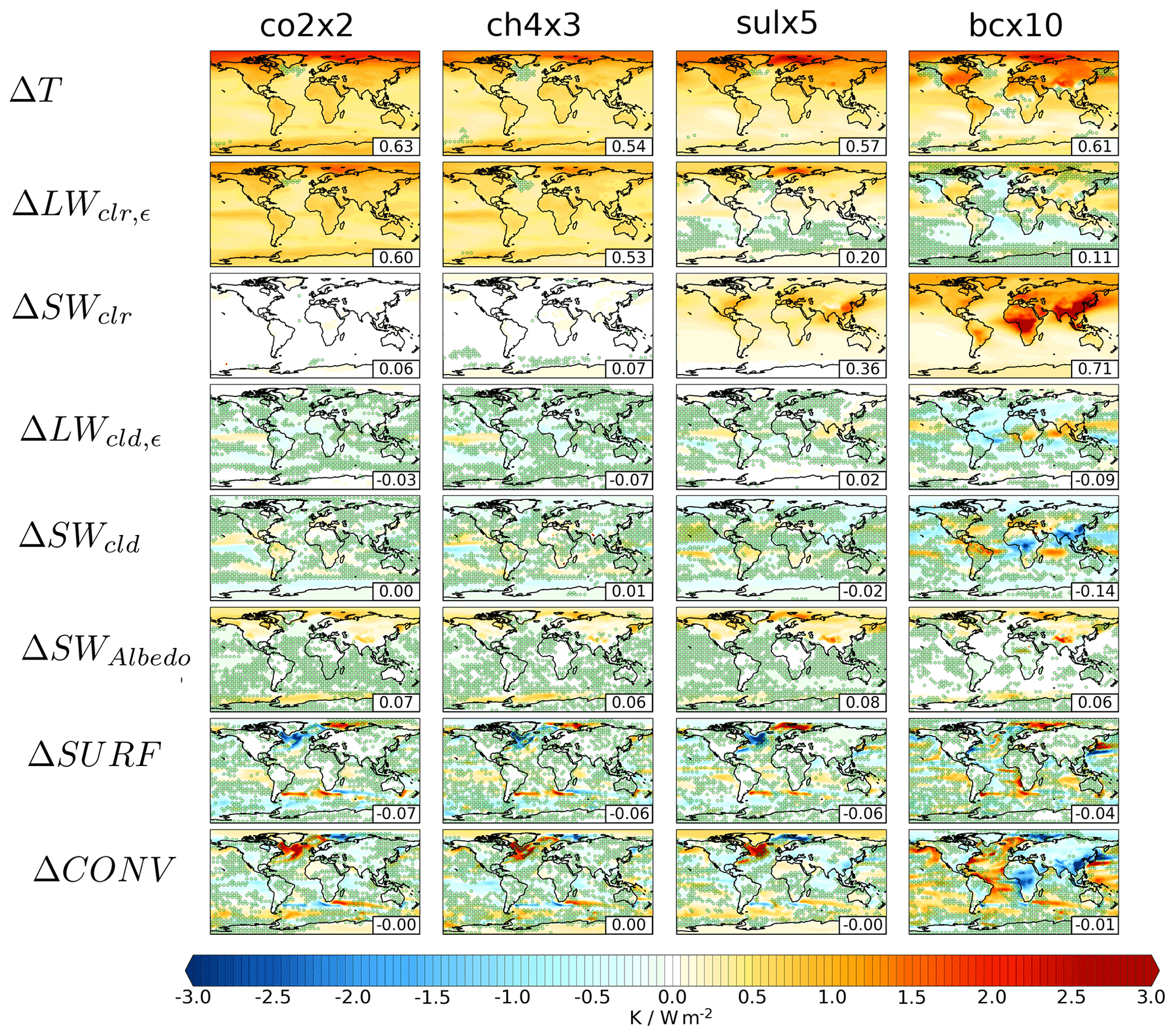
Figure 4 The multimodel-mean effective temperature response (row 1) for four different climate forcers, i.e., carbon dioxide (column 1), methane (column 2), sulfate (column 3), and black carbon (column 4), and its decomposition into different energy balance terms (long- and shortwave clear-sky (ΔLW_clr, ΔSW_clr), clouds, surface energy exchange (ΔSURF), and horizontal energy transport (ΔCONV)). Dotted areas show regions where only 4 out of the 6 models agree on the sign of the response.

The spatial distribution of the total effective temperature response is largely similar for each forcer, although the total response to aerosols is stronger over the continental northern midlatitudes, compared to total responses to greenhouse gases, and weaker over the Southern Hemisphere oceans. Regionally, local maximum effective temperature responses are found in the Barents Sea for all forcers, with maximum values of 2.38, 2.04, 2.96, and 2.53 K W⁻¹ m² for co2x2, ch4x3, sulx5 and bcx10, respectively. This is most visible in the LW clear-sky term. Stejrn et al. (2019) showed that the largest local temperature responses in PDRMIP experiments are in regions with the largest sea-ice changes. Differences between forcers can be seen, for example, over the Antarctic region where both greenhouse gas experiments (ch2x2, ch4x3) produce Antarctic amplification which is not seen in the aerosol experiments. The effective temperature responses in the bcx10 experiment show higher contrasts between land and sea regions than in the other experiments.

For greenhouse gases, the regional effective temperature responses are mostly associated with the response to ΔLW_clr. However, with all forcers the spatial distribution of the ΔLW_clr contribution resembles the overall effective temperature response. The spatial correlation coefficients between the effective total and ΔLW_clr-induced temperature responses for the co2x2, ch4x3, sulx5, and bcx10 experiments are 0.90, 0.81, 0,94, and 0.74, respectively. The difference between the greenhouse gas and aerosol experiments is that for greenhouse gases the ΔLW_clr response includes the combined effects of forcing, its rapid adjustments and lapse rate, and water vapor feedbacks, while for aerosols the response results only from the rapid adjustments and lapse rate and water vapor feedbacks. For the co2x2 and ch4x3 experiments, the total effective temperature response and ΔLW_clr temperature response differ most in the equatorial Pacific Ocean, where the ΔLW_clr response exceeds the total response. The high ΔLW_clr temperature response in this region is compensated by contributions from ΔSW_cld, ΔLW_cld, and atmospheric energy transport ΔCONV (see Fig. 4).

For aerosols, most of the effective temperature response is due to ΔSW_clr. Besides the modest water vapor contributions to ΔSW_clr, this response is directly related to excess scattering and absorption of solar radiation (direct aerosol radiative forcing) due to changes in aerosol concentrations, as was shown in Merikanto et al. (2021). Most of the sulfate emissions originate from Asia, Europe, and North America, while most of the black carbon emissions originate from Asia, Europe, and North America as well as African, South American, and boreal wildfires (Myhre et al., 2013), This makes the forcing in both cases stronger in the Northern Hemisphere than in the Southern Hemisphere. The ΔSW_clr temperature response to these emissions can be clearly seen both for the bcx10 and sulx5 experiments (see Fig. 5). For the bcx10 experiments, the local effective temperature response due to ΔSW_clr exceeds the total effective temperature response from the tropics to the northern midlatitudes (Fig. 5). These local excess warming responses by ΔSW_clr in bcx10 experiments are counteracted by temperature responses to changes in atmospheric energy transport and clouds. In the case of aerosols, ΔLW_clr contributes to the effective temperature response mainly in the Northern Hemisphere continents and Arctic sea-ice regions. In the bcx10 experiments, ΔLW_clr induces a clear negative contribution over ocean regions related to changes in the vertical temperature distribution of the atmosphere (see Fig. S2). The top-heavy warming in bcx10 experiment results from fast adjustments as shown in Smith et al. (2018), where BC absorbs incoming SW radiation, leading to warming of the upper atmosphere and increasing low-level clouds. Furthermore, over oceans there is more moisture available for low-level cloud formations, leading to cooling of the surface.

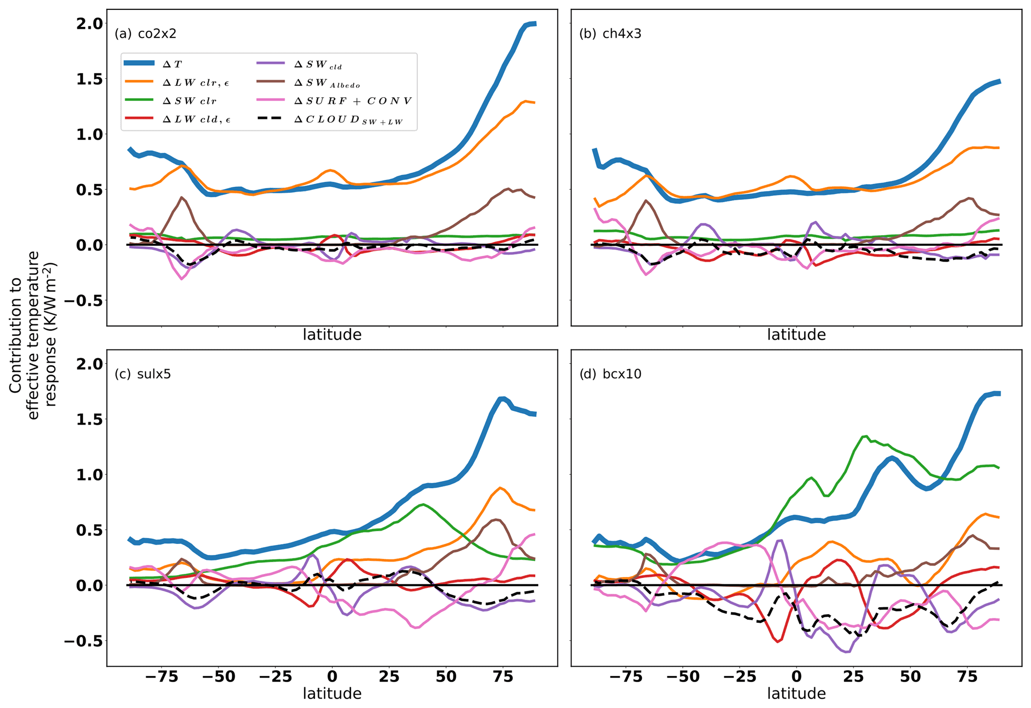
Figure 5 Zonal-average multimodel-mean effective temperature response (thick blue lines) and its decomposition into different energetic terms (thin colored lines) for different climate forcers. Panel (a) shows co2x2, panel (b) shows ch4x3, panel (c) shows sulx5, and panel (d) shows bcx10.

There is significant variation in the regional effective temperature contributions due to clouds between regions and forcing agents. In the greenhouse gas experiments (co2x2 and ch4x3), the regional effective temperature responses due to ΔLW_cld and ΔSW_cld tend to cancel each other, except over the Southern Ocean where the total cloud contribution is dominated by a negative ΔSW_cld (see Fig. 5). This relates to a strong increase in cloud cover in the same regions (see Figs. S4 and S5).

With aerosols, the net effect of clouds is more complicated. Both the sulx5 and bcx10 experiments show a similar negative effective temperature response due to ΔSW_cld over the Southern Ocean as the greenhouse gases. However, northern hemispheric cloud responses are larger in magnitude for aerosols than for greenhouse gases, particularly for the bcx10 experiment. Throughout all latitudes bcx10 causes a strong net cloud cooling, except for the polar regions where the net cloud responses are small. The sign of the regional ΔSW_cld effective temperature response in the bcx10 experiments depends strongly on the region. There is a negative temperature response due to ΔSW_cld in Asia and Africa but positive over the Amazon region. This is related to the cloud cover change, as black carbon increases the cloud cover over Asia and Africa but decreases it over the Amazon (see Fig. S5) due to the semidirect aerosol effect of black carbon. Contrary to bcx10, sulx5 shows a mild positive contribution from clouds over northern hemispheric midlatitudes and a mild cooling response in the Arctic regions. However, the strength of the ΔSW_cld responses in the sulx5 experiments depends on the inclusion or lack of the aerosol–cloud indirect effect in the models.

The effective temperature response to surface albedo change originates from the change in sea-ice and snow cover and is always positive. Changes in surface albedo have a modest effect on the global effective temperature response with all forcers (0.07, 0.06, 0.08, and 0.06 K W⁻¹ m² for the co2x2, ch4x3, sulx5, and bcx10 experiments, respectively). However, in some regions, the effective temperature response to albedo change exceeds 1 K W⁻¹ m² for all forcers. Over the Arctic, the regions of local maximum values are the same where the overall effective temperature responses are highest, highlighting the role of sea-ice changes causing locally high temperature responses. The local maximum values of the effective temperature response to albedo change also match with the regions with a positive temperature response to ocean heat exchange (ΔSURF). The change in surface albedo also enhances the temperature response over the Southern Ocean, but there the temperature response to oceanic heat exchange is slightly negative. However, over the Southern Ocean the temperature response signal to surface albedo change is mainly visible in the co2x2 and ch4x3 experiments and appears to be driven by the longwave clear-sky forcing and feedbacks and ocean heat transport.

Over the oceans, ΔSURF has a large impact on the effective temperature response, with the co2x2, ch4x3, and sulx5 experiments all showing negative effective temperature contributions due to ΔSURF south of Greenland and positive contributions over the Barents Sea. With black carbon, a robust negative signal over the northern North Atlantic is missing, however, but similarly to other forcers, there is a robust positive signal over the Barents Sea. As earlier found for increased CO₂ by Räisänen (2017), the effects of oceanic heat transport and storage (ΔSURF) and atmospheric heat transport (ΔCONV) strongly oppose each other over the oceans in the co2x2, ch4x3, and sulx5 experiments. In the sulx5 and bcx10 experiments, ΔCONV also significantly compensates for the surface temperature effects due to changes in ΔSW_clr, which reflects changes in the direct aerosol forcing.

3.3 Model-to-model spread in regional effective temperature responses for different forcers

Similarly to the effective temperature response itself, also its model-to-model spread (standard deviation) can be decomposed into components that sum up to the total spread in the effective surface temperature response (Sect. 2.2). Figure 6 shows the decomposed model-to-model standard deviations of the total effective temperature responses (first row) for each perturbation experiment and the decomposed contributions of each component to the spread in total responses. The latitudinal distributions of the different components are shown in Fig. 7.

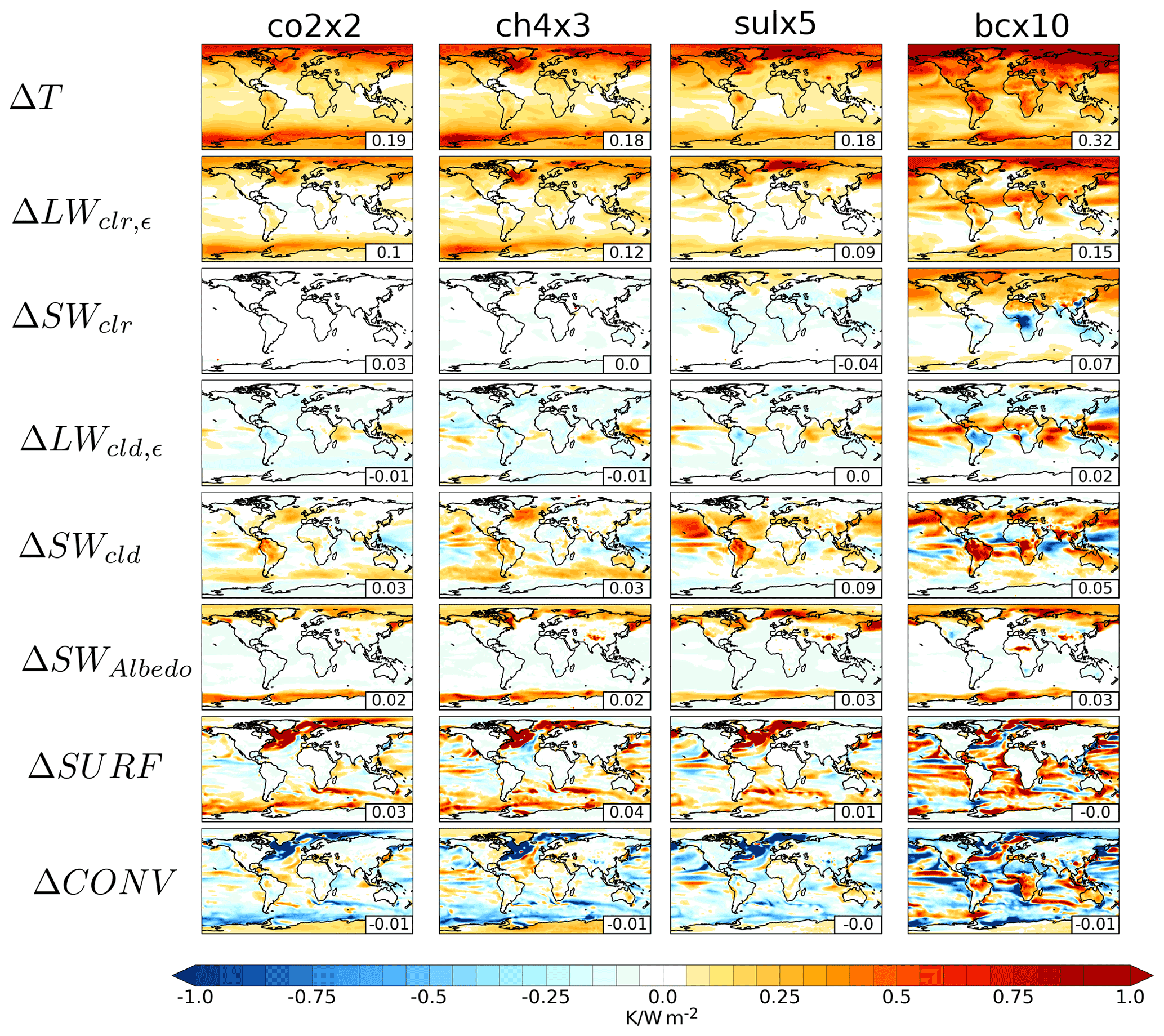
Figure 6 The model-to-model standard deviation of the effective temperature response to different climate perturbations (row 1) and its decomposed different energetic components (rows 2–8). Each column shows results for four different climate forcers, i.e., carbon dioxide (column 1), methane (column 2), sulfate (column 3) and black carbon (column 4). The global mean values are shown at the bottom right corner of each panel.

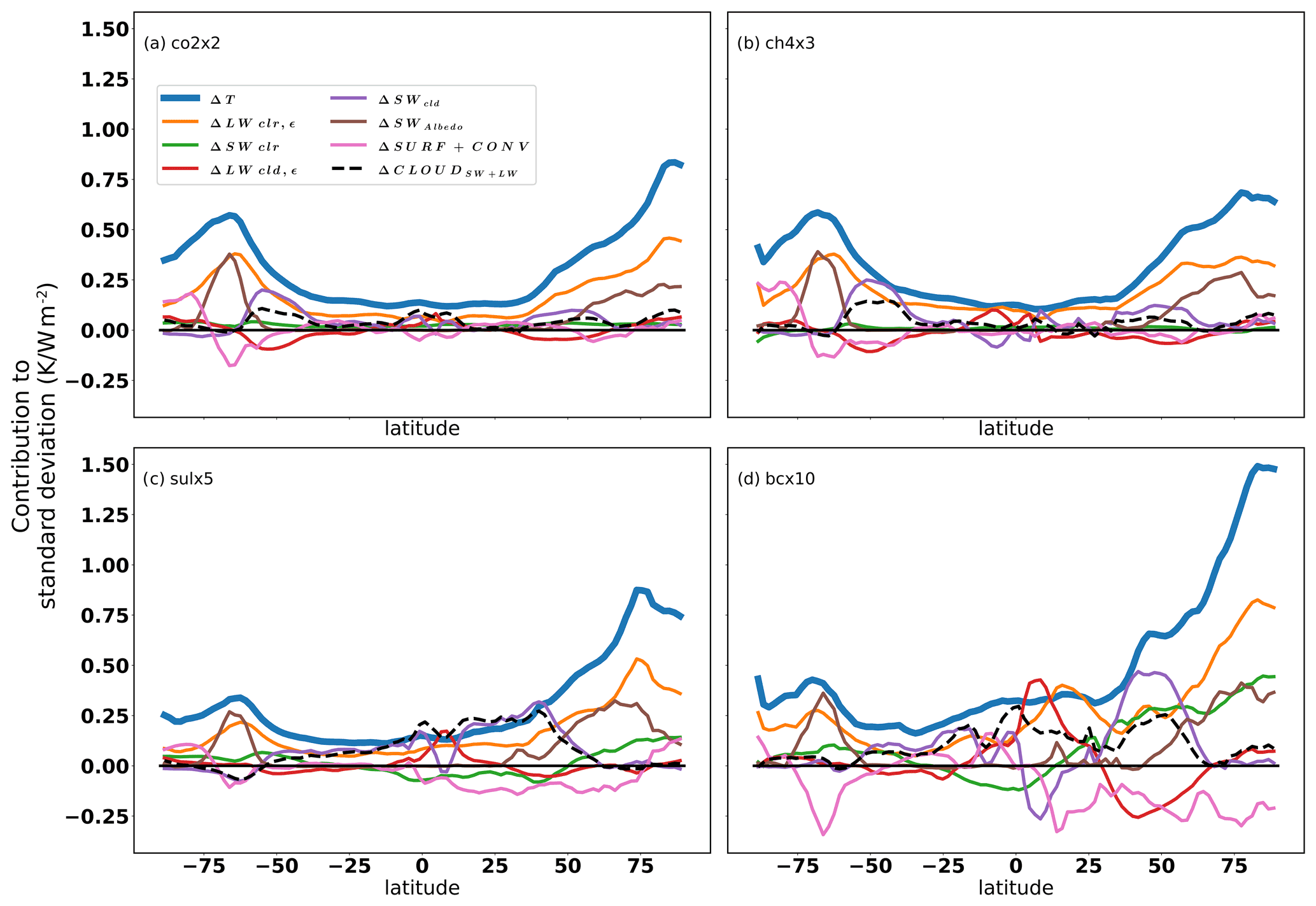
Figure 7 Zonal mean of the total standard deviation of the effective temperature response (thick blue line) and the contributions of the different energy balance terms to it (thin lines; see the legend in a). Panel (a) shows co2x2, panel (b) shows ch4x3, panel (c) shows sulx5, and panel (d) shows bcx10.

The globally averaged magnitude of the model-to-model spread is similar between co2x2, ch4x3, and sulx5 experiments (0.19, 0.18, and 0.18 K W⁻¹ m², respectively). Black carbon induces a much larger variability between the models (0.32 K W⁻¹ m²). The spatial structure of the model-to-model spread resembles the spatial structure of the effective temperature response. Furthermore, the spread in the temperature response amplifies towards polar regions, but the polar amplification of the spread is even stronger than the amplification of the responses. Indeed, the majority of the model spread comes from the sea-ice regions in the high latitudes, but the location of the maximum model-to-model spread varies between forcers. With co2x2 and ch4x3, the regions with highest model spread are in the Arctic Ocean region north of Siberia (1.10 K W⁻¹ m² with co2x2 and 1.30 K W⁻¹ m² with ch4x3) and in the Labrador Sea (0.90 K W⁻¹ m² with co2x2 and 1.60 K W⁻¹ m² with ch4x3). With sulfate, the spread is the largest in the ocean region between Iceland and Svalbard (2.47 K W⁻¹ m²) and for black carbon east of Svalbard (2.23 K W⁻¹ m²). In the co2x2 and ch4x3 experiments, the strongest component in model-to-model spread is ΔLW_clr (see Fig. 7), but the partial contributions of other components are also significant. The amplification of the spread in the effective temperature response towards high latitudes (Fig. 7) is strongly related to additional spread arising from differences in the surface albedo response (ΔSW_Albedo), reflecting differences in sea-ice and snow cover responses. The total contributions of cloud responses to the model spread are significant over southern and northern midlatitudes and to a lesser extent over the equatorial region. In the Southern Ocean sea-ice regions, the model spread originates from differences in the ΔLW_clr and ΔSW_Albedo responses in the models, as well as from differences in the oceanic heat exchange (ΔSURF) compensated by differences in the atmospheric heat transport (ΔCONV) (see Fig. 6). Between 30–45^∘ S, the model spread due to the combined effect of clouds (ΔSW_cld+dΔLW_cld) is also evident. However, in the co2x2 and ch4x3 experiments the ΔSW_cld and ΔLW_cld terms often oppose each other, thus making the combined contribution of clouds to the total model spreads small in these experiments.

In the aerosol experiments (sulx5 and bcx10) the build-up of the model-to-model spread is more complicated than for the greenhouse gas experiments, despite similarities in the latitudinal distribution of the total spread of the effective temperature response. The contributions of ΔSW_clr (the pathway of aerosol direct radiative forcing) and the combined cloud response (ΔSW_cld+ΔLW_cld) to the total model spread are much more significant in the aerosol experiments than in the greenhouse gas experiments. In the aerosol experiments, ΔSW_clr adds to the model spread over the Southern Ocean in both the sulx5 and bcx10 experiments, suppresses the model spread over midlatitude and equatorial oceans in sulx5 and over Southern Hemisphere and equatorial continents in bcx10, and adds model spread over northern hemispheric continents (bcx5) and over the Arctic Ocean (both sulx5 and bcx10). Clouds have a large impact on the regional model-to-model spread in the aerosol experiments and dominate the zonal means of the model spread in the sulx5 experiments outside of the polar regions. Much of the model spread related to the combined cloud contributions (ΔSW_cld+ΔLW_cld) results from differences in the aerosol setups in the models. With aerosol experiments (sulx5 and bcx10), most of the cloud-induced model-to-model spread is related to emissions sources and is highly affected by which aerosol–cloud effects are included in the models. Also for aerosols, the contributions to model spread due to ΔSW_cld and ΔLW_cld often oppose each other, but the stronger model spread related to the ΔSW_cld response dominates the overall cloud contribution in midlatitudes, while model spread due to ΔLW_cld dominates the model spread over the equatorial regions.

On the other hand, in the aerosol experiments (sulx5 and bcx10) the atmospheric heat transport (ΔCONV) tends to compensate the regional differences in model responses more efficiently than in the greenhouse gas experiments. In addition, the total heat transport (ΔSURF + ΔCONV) reduces the zonally averaged model spread (see Fig. 7), particularly in the case of the bcx10 experiments. Similarly to the greenhouse gas experiments, ΔLW_clr is still a major driver of model-to-model spread also in the aerosol experiments and particularly in the high-latitude regions (Fig. 6). Compared to the greenhouse gas experiments, the aerosol experiments exhibit much greater contributions from ΔSW_Albedo to the overall model-to-model spread in the Arctic region. In the co2x2 and ch4x3 experiments, the maximum contributions to the model spread in the Arctic due to ΔSW_Albedo are 0.23 and 0.29 K W⁻¹ m², respectively, while for sulx5 and bcx10 the corresponding values are 0.32 and 0.41 K W⁻¹ m², respectively. In the Southern Hemisphere high latitudes, aerosols and greenhouse gases have a similar structure in model-to-model variability; however, the aerosol experiments do not show a clear signal from ΔSW_cld in the Southern Ocean.

Previously, the model-to-model spread in global climate sensitivity (equilibrium response to doubled CO₂ concentration) has been largely attributed to differences in cloud feedback strength (Colman, 2003; Zelinka et al., 2020; Zhao et al., 2016). Our results point to somewhat divergent conclusions. Similarly to Hu et al. (2020), our results point to the water vapor feedback as the main mechanism leading to model spread. If the model spread is only attributed using feedback analysis, model differences in the forcing and adjustments may counteract some of the differences. However, it should be noted that our results are based on only six different models and hence might be biased. For example, Zelinka et al. (2020) show that the contribution of clouds to the equilibrium climate sensitivity response exhibits notably large variation from approximately −0.2 to 3 K for CMIP6 models and −0.18 to 2.6 K for CMIP5. In our results, ΔSW_cld and ΔLW_cld largely cancel each other out in the co2x2 experiments, leading to a smaller combined cloud contribution to the model spread and contributes only 12 % (see Table S1) to the global model spread. For comparison, for a sample of 16 CMIP5 models with a transient response to doubling of CO₂, Räisänen (2017) found the clear-sky LW response to be the largest contributor to the model spread in 34 % of the global area, whereas the combined cloud response had this position in 29 % of the world.

4 Discussion and conclusions

In this work, we have conducted an energy balance decomposition of the near-surface temperature response resulting from doubling CO₂, tripling CH₄, 5-fold increasing sulfate concentrations, and 10-fold increasing black carbon concentrations for six independent climate models. The regional temperature response was then decomposed into contributions from different energy balance terms, namely, changes in LW and SW clear-sky and cloud radiative fluxes (SW and LW), the net surface energy flux (SURF), and horizontal energy transport (CONV). All forcers produce a similar global response per unit ERF (0.63, 0.54, 0.57 and 0.61 K W⁻¹ m² for increasing CO₂, CH₄, sulfates, and black carbon, respectively). The majority of the globally averaged temperature change for doubling the CO₂ and tripling the CH₄ concentration originates from changes in clear-sky planetary emissivity (0.60 and 0.53 K W⁻¹ m², respectively), i.e., from the combination of the longwave clear-sky radiative forcing with the change in the thermal structure of the atmosphere and water vapor concentrations. In the aerosol experiments (sulfate and black carbon), the key driver of surface temperature response is the change in the clear-sky shortwave radiative flux (0.36 and 0.71 K W⁻¹ m², respectively) related to excess scattering and absorption of solar radiation (direct aerosol radiative forcing) due to changes in aerosol concentrations. We note that if only models including sulfate aerosol–cloud interactions are included, the SW cloud terms are in the same magnitude (ΔSW_clr=0.25 and ΔSW_cld=0.12 K W⁻¹ m²). See below for a more detailed discussion on different aerosol setups. The overall temperature response to the forcers is largest in high latitudes, where the response is driven by changes in LW clear-sky fluxes and changes in surface albedo, except for black carbon for which the majority of the total response comes from the clear-sky SW term in the high latitudes.

The temperature decomposition method provides a tool for understanding regional and global temperature changes. However, the original method is somewhat simplistic in its treatment of LW cloud processes (Räisänen, 2017). In Merikanto et al. (2021), we implemented a radiative kernel correction to make the LW treatment of clouds more realistic. However, despite this correction, we still have a negative effective LW temperature response from clouds when the CO₂ concentration is doubled, whereas literature suggests a positive LW cloud feedback (Tomassini et al., 2013; Vial et al., 2013). This is due to neglecting the positive masking effect of increasing CO₂ on the LW cloud forcing, since the corresponding effects can not be calculated for the other forcing agents with existing kernels. The applied radiative kernels for temperature and H₂O have a relatively minor effect on global averages of the LW cloud and clear-sky terms (see Fig. S6). Similarly to previous studies (Smith et al., 2018), we found that the relative importance of the kernel correction does not depend on the radiative kernel used.

In our study, clouds play a minor role in the global mean temperature response, as the LW cloud and SW cloud terms tend to cancel each other out. However, regionally the temperature response originating from the clouds is a significant contributor. For all forcers, the temperature response in the Antarctic sea-ice region and in the Southern Ocean is dampened by clouds. With BC, clouds dampen the regional temperature response in Asia, North America, Africa, and Europe and enhance the warming in the Amazon. In contrast to clouds, with all forcing agents surface albedo changes enhance the temperature responses in high latitudes. For greenhouse gases, the mild polar amplification in the south is associated with a negative contribution from the ocean heat exchange over the Southern Ocean, negative total cloud contribution and a mild LW clear-sky component.

We also decompose the model-to-model spread into the contributions of energy balance terms. The model-to-model spread is the largest in the same regions as the average temperature response, i.e., at high latitudes, where the spread is driven by differences in the lapse-rate and water vapor feedbacks (ΔLW_clr) and differences in surface albedo (ΔSW_Albedo) changes. For the aerosol-induced temperature responses, also differences in the direct aerosol forcing (ΔSW_clr) generate a significant contribution to the model spread, especially for black carbon. This partly arises from different aerosol configuration between models.

The aerosol configuration is important in the generation of the effective temperature response and its model-to-model spread. In the aerosol experiments, part of the model-to-model spread originates from the difference between aerosol setups, with the emission-driven models generating a higher effective temperature response than the concentration-driven models. For sulx5, the concentration-driven models' mean effective temperature response is 0.49 K W⁻¹ m², while for the emission-driven models it is 0.66 K W⁻¹ m². The corresponding numbers for the bcx10 experiments are 0.45 and 0.76 K W⁻¹ m². For the sulx5 experiments, the sign and the regional distribution of ΔSW_cld is strongly related to the aerosol setup; however, it should be noted that two out of the three concentration-driven models do not include aerosol–cloud interactions. In the bcx10 experiment, the aerosol setup modifies the ΔSW_clr and ΔLW_clr temperature responses (see Fig. S1, showing the decomposed temperature responses separately for the concentration and emission-driven models for the sulx5 and bcx10 experiments). The aerosol configuration also plays a crucial role in the SW albedo response. For both the sulx5 and bcx10 aerosol experiments, only the emission-driven models show a significant temperature contribution from the ΔSW_Albedo term (0.1 and 0.08 K W⁻¹ m², respectively), whereas the corresponding mean values for the concentration driven models are only 0.06 and 0.03 K W⁻¹ m².

We have demonstrated that the mechanisms behind model uncertainty vary between different regions and forcing agents. Understanding the atmosphere's dynamical response to different forcers is key to understanding future climate changes at the regional level. This is especially important in the case of aerosols, which are predicted to decline in the near future due to climate change and air pollution mitigation actions.