Surface deposition of marine fog and its treatment in the Weather Research and Forecasting (WRF) model

There have been many studies of marine fog, some using Weather Research and Forecasting (WRF) and other models. Several model studies report overpredictions of near-surface liquid water content (Q_c), leading to visibility estimates that are too low. This study has found the same. One possible cause of this overestimation could be the treatment of a surface deposition rate of fog droplets at the underlying water surface. Most models, including the Advanced Research Weather Research and Forecasting (WRF-ARW) Model, available from the National Center for Atmospheric Research (NCAR), take account of gravitational settling of cloud droplets throughout the domain and at the surface. However, there should be an additional deposition as turbulence causes fog droplets to collide and coalesce with the water surface. A water surface, or any wet surface, can then be an effective sink for fog water droplets. This process can be parameterized as an additional deposition velocity with a model that could be based on a roughness length for water droplets, z_0c, that may be significantly larger than the roughness length for water vapour, z_0q. This can be implemented in WRF either as a variant of the Katata scheme for deposition to vegetation or via direct modifications in boundary-layer modules.

1 Introduction

This study was initiated when it was found that predicting fog in areas offshore from Atlantic Canada using the National Center for Atmospheric Research and University Corporation for Atmospheric Research (NCAR/UCAR) Weather Research and Forecasting model (WRF-ARW) was generally satisfactory in terms of fog occurrence but gave high values of cloud water mixing ratio, leading to visibilities that were too low compared to observations. Other studies of marine fog had encountered similar problems (e.g. Chen et al., 2020). Koračin et al. (2014) had noted that, “From the many modeling studies of sea fog, essentially numerical experiments/simulations/forecasting that started in the immediate post WWII period, it becomes clear that deterministic forecasting of sea fog onset and its duration has generally been unsuccessful”. On land and over the sea, the formation and decay of fog in the atmospheric boundary layer is a complex issue involving many processes including cloud microphysics, longwave and solar radiation, turbulent boundary layer mixing, advection and surface interactions. Modelling of fog, in idealized one dimensional or single column models up to operational 3-D weather prediction and climate models, is a challenge which many have addressed over the years, as noted by Koračin (2017), Gultepe et al. (2017) and many others. Koračin et al. (2014) review marine fog processes and studies up to 2014, noting the importance of air–sea interactions. They discuss fog water deposition to vegetation extensively but not turbulent deposition to water surfaces, and it is missing from their Fig. 1 (and Fig. 9.1 in Koračin, 2017) which shows “the main processes governing the formation, evolution, and dissipation of marine fog”. Although fog could be caused by mixing two slightly subsaturated air parcels and causing saturation due to curvature of the saturated mixing ratio versus temperature line, most fog formation is initialized by cooling the lower parts of a column of moist, but unsaturated, air. This can arise because of longwave radiative heat loss from the underlying surface (radiation fog), vertical displacement of the air column as it travels over sloping terrain or horizontal advection over a cooler surface. Our focus is on the advection fog situation over ocean waters, a frequent occurrence over areas such as the Grand Banks and offshore areas of eastern Canada as the wind blows moist air from over the Gulf Stream towards the Labrador Current (Taylor 1917; Isaac et al., 2020).

1.1 Fog and the underlying surface

The focus in this paper is on the interactions of fog water droplets with the underlying water surface, how this is being modelled and how it could be improved in the widely used WRF model, and it will briefly suggest some field measurements to support this work. The basic hypothesis will be that, in addition to gravitational settling, turbulence will induce collisions between fog droplets and the water surface, and that most of these collisions will lead to coalescence, so that the water surface is a sink for water droplets. This can be represented in terms of a deposition velocity over and above the settling or terminal velocity associated with small cloud droplets falling through the air under gravity, which is predictable assuming Stokes law (see, for example, Rogers and Yau 1989). Different authors use different symbols (Q_c, q_w, LWC, w, etc.) and different measures (grams per kilogram, hereafter g kg⁻¹; kilograms per cubic meter, hereafter kg m⁻³; etc.) of fog or cloud water content. We will use Q_c for mixing ratio (g kg⁻¹ or kilograms per kilogram, hereafter kg kg⁻¹) and LWC=ρ_aQ_c, where ρ_a is air density, as liquid water content (kg m⁻³ or grams per cubic meter, hereafter g m⁻³) unless discussing results from specific papers where, for clarity, it is sometimes useful to use their symbols. If there is an enhanced turbulent deposition to the water surface, one would then expect the cloud water mixing ratio (Q_c) to approach zero at the surface and increase with height (z) above the surface. In a constant flux layer, this would lead to a logarithmic profile and allow the concept of a roughness length for cloud droplets, z_0c, although the profile can be modified to incorporate gravitational settling (Taylor, 2021). Not included is the possible creation of spray droplets by breaking waves in high wind speeds, and this may need consideration in high seas with strong winds.

There have been many studies on the collision and coalescence of raindrops and cloud droplets, and of droplets impacting hydrophobic surfaces, but relatively few concerning interactions between cloud or fog droplets and ocean surfaces. Over water, the combination of wind and waves will lead to impacts occurring at a range of speeds and incidence angles, and relatively little is known about the details of this important interaction. The paper by Hallett and Christensen (1984) and the reference to it by Isaac and Hallett (2005), although primarily focused on impacts at normal incidence, do, however, support our expectation that fog droplets interacting with the ocean surface are likely to coalesce eventually, even if they may bounce on initial impact if that occurs at a shallow angle. If fog droplets do collide with the underlying surface, whether it is the ocean, a lake, a water puddle on land or wet vegetation, one would expect coalescence and deposition of the fog droplets to the surface. Gravitational settling will play a role in this, but droplet impacts on the surface due to turbulence also need to be considered. As a result of deposition, there would be a reduction in the fog–cloud water mixing ratio (Q_c), maybe to zero, at the lower boundary, which would lead to a positive value for dQ_c/dz and a downward flux of Q_c.

1.2 Aerosol and vegetation

If we broaden our view and consider aerosols in general, we find that significant work has been done in the same size range as fog droplets (1–50 µm). Recent reviews by Emerson et al. (2020) and Farmer et al. (2021) make it very clear that dry deposition (i.e. not rainfall related) of aerosol particles, solid or liquid, is a key process for their removal, and that it is driven by turbulence and strongly dependent on particle size. For aerosol with diameters>1 µm gravitational settling and turbulent diffusion, both contribute to the overall deposition velocity. The aerosol studies include both water surfaces and vegetation. It is clear from Farmer et al. (2021; Fig. 3) that deposition velocity, V_dep, over water increases significantly with aerosol diameter between 1 and 50 µm, while this variation is somewhat less over other surfaces. Farmer et al.'s (2021) plots are not normalized by friction velocity or wind speed, which probably accounts for some of the variability in V_dep at fixed diameters.

There have been studies of fog deposition to vegetation and also to meshes designed to catch fog water (e.g. Sect. 3.4 of Gultepe et al., 2017). However, as far as we are aware, the models of fog droplet deposition to water surfaces have either been via gravitational settling alone, ignored or considered as a part of a turbulent total water (vapour, q, plus liquid droplets) flux at the surface. Right at the surface, the flux of water vapour will rely on molecular transfer alone while the collision and coalescence of water droplets can be much more efficient and require separate treatment.

2 Boundary layer modelling

For aerosols and sometimes other quantities, weather prediction and other models tend to use deposition velocities (V_dep) to relate fluxes to an underlying surface to concentrations at some level above the surface. From a boundary layer perspective, one often looks at the concentration profile and an eddy diffusivity. The simplest, and traditional, way to model the flux profile relationships of a quantity, s, in neutrally stratified, turbulent boundary layer flow near rough walls is via an eddy viscosity/diffusivity, $K_s\left(z\right)=k{u}_{*}(z+z_{\text{0s}})$, where k is the Kármán constant (0.4), and u_* is the friction velocity. The roughness length, z_0s, is specific to the property (horizontal velocity, temperature, mixing ratio, …) under consideration and will vary considerably, depending on the physics of the final transfer process at the surface. The traditional way to determine z_0s is to consider an approximately constant flux layer near the surface, leading to a logarithmic profile, as follows:

$$\begin{array}{}\text{(1)}& S-S_{\mathrm{0}}\approx (s_{*}/k)\log (z/z_{\text{0s}}),\end{array}$$

where S₀ is the surface value. This will imply that S=S₀ at z=z_0s and is the empirical way in which z_0s can be determined. It is well known, see, for example, Garratt (1992) or Brutsaert (1982), that roughness lengths for momentum (z_0m) and heat or water vapour (z_0T,z_0q) transfers differ because form drag on roughness elements is the major cause of momentum transfer, while molecular diffusivity at the surface is needed to effect heat transfer. As a result, z_0m≫z_0q, except maybe over aerodynamically smooth surfaces. We will propose the use of z_0c for cloud droplet collision and coalescence with the water surface. We have no measurement data to determine a value, which might well vary with droplet size and sea state, but we can use reported aerosol studies to provide some guidance. We do, however, expect that z_0c≫z_0q.

If the fog has continued for some time, one might expect that the relative humidity, RH, is equal to 100 % in the fog layer, with no significant condensation or evaporation. There will then be a near-steady state in the lower fog layers with constant downward Q_c flux ($F_{Q_{\mathrm{c}}}$). This flux will be a combination of turbulent diffusion and gravitational settling (w_sQ_c), where w_s is the gravitational settling velocity, based on Stokes law. If, as we will assume, Q_c→0 as z→0, then turbulent transfer will dominate as the surface is approached, and logarithmic Q_c profiles should result.

In our model calculations, with an eddy diffusivity, $K_{\mathrm{c}}\left(z\right)=k{u}_{*}(z+z_{\text{0c}})$, we do find RH≈100 % in the fog layers, typically up to around 100 m, and we see constant flux layers with near-logarithmic Q_c profiles through most of this height range, as in Fig. 4. Departures from logarithmic profiles could arise in part due to the effects of gravitational settling.

Marine fog in the areas under consideration often occurs in moderate and high wind conditions (Isaac et al., 2020). Relatively low heights (<10 m) are used as the lowest model level, and in that lowest, constant flux wall layer with neutral stratification, we can assume horizontal homogeneity, a constant downward flux of Q_c and a steady state. We can then seek the solution to the following:

$$\begin{array}{}\text{(2)}& w_{\mathrm{s}}{Q}_{\mathrm{c}}+k{u}_{*}(z+z_{\text{0c}})\mathrm{d}{Q}_{\mathrm{c}}/\mathrm{d}z=F_{Q_{\mathrm{c}}}=u_{*}{q}_{\text{c*}},\end{array}$$

where $F_{Q_{\mathrm{c}}}$ is a downward flux of cloud droplet liquid water mixing ratio, and q_c* is introduced as a mixing ratio scale. With $Q_{\mathrm{c}}=Q_{{\mathrm{c}}_{\mathrm{0}}}$ at z=0, the solution is as follows:

$$\begin{array}{ll}{\displaystyle }& {\displaystyle }{Q}_{\mathrm{c}}\left(z\right)-Q_{{\mathrm{c}}_{\mathrm{0}}}=(u_{*}{q}_{c*}/w_{\mathrm{s}})\left[\mathrm{1}-\exp \left(-w_{\mathrm{s}}\mathit{\zeta }/\left(k{u}_{*}\right)\right)\right],\\ \text{(3)}& {\displaystyle }& {\displaystyle }\text{where}\mathit{\zeta }=\ln \left(\left(z+z_{\text{0c}}\right)/z_{\text{0c}}\right).\end{array}$$

If $w_{\mathrm{s}}/u_{*}$ is small, then to first order in $w_{\mathrm{s}}\mathit{\zeta }/k{u}_{*}$, Eq. (3) simply becomes the following:

$$\begin{array}{ll}{\displaystyle }& {\displaystyle }{Q}_{\mathrm{c}}\left(z\right)-Q_{{\mathrm{c}}_{\mathrm{0}}}=\left(q_{c*}/k\right)\ln \left(\left(z+z_{\text{0c}}\right)/z_{\text{0c}}\right),\\ \text{(4)}& {\displaystyle }& {\displaystyle }\text{with}{Q}_{\mathrm{c}}=Q_{{\mathrm{c}}_{\mathrm{0}}}\text{at}z=\mathrm{0}.\end{array}$$

If this is used to relate z_0c to a deposition velocity, V_d, and with $Q_{{\mathrm{c}}_{\mathrm{0}}}=\mathrm{0}$, we would have the following:

$$\begin{array}{}\text{(5)}& V_{\mathrm{d}}=u_{*}k/\ln \left(\left(z_{\mathrm{1}}+z_{\text{0c}}\right)/z_{\text{0c}}\right),\end{array}$$

where z₁ is the height above the surface where Q_c is measured. This logarithmic profile approximation could be fit to measured Q_c profiles to determine z_0c from observations. As with z_0m, this is a somewhat empirical approach. In the same way that the use of the z_0m concept is widely accepted without precise calculation of the form drag on roughness elements, we would hope that future experimental determination of z_0c would be a way to account for the effects of turbulent collision and coalescence of fog droplets with a water surface. For radiation fog in low wind speeds over land, stable air density stratification effects could be significant and can be accounted for with Monin–Obukhov similarity modifications to K_c(z,L), if the Obukhov length (L) can be determined.

The expected values of terminal velocity, w_s, for a droplet of diameter, d, and density, ρ, falling under gravity (g) through air of density, ρ_a, and molecular viscosity, μ, should be considered. In reality, the fog droplet size distribution will be broad and often bimodal (see Isaac et al., 2020). The two peaks in some of Isaac et al.'s (2020) measured droplet size distributions are at diameters near 6 and 25 µm, with Stokes law terminal velocities ($w_{\mathrm{s}}=g{d}^{\mathrm{2}}(\mathit{\rho }-{\mathit{\rho }}_{\mathrm{a}})/\mathit{\mu }$) of 0.001 and 0.019 m s⁻¹. These are clearly small compared to wind speed, but for the larger diameter, where the bulk of the liquid water content (LWC) is often measured, the terminal velocity corresponds to 67 m h⁻¹ and will represent a considerable removal rate in fog which may last several days. The key parameter in our constant flux with gravitational settling model is $S=w_{\mathrm{s}}/k{u}_{*}$. In moderate winds over the ocean, one might expect u_* values in the 0.1–0.5 m s⁻¹ range, k=0.4 and so the parameter, S, will generally be in the range 0.006 to 0.46, while ζ may be 5–10 at the lowest grid point, implying that gravitational settling can play a significant role, and that Eq. (3) may provide a more appropriate profile for the larger droplets. In principle, Eq. (3) should be used to refine any z_0c estimates from measurements. For typical friction velocities (0.1–0.5 m s⁻¹) and with the lowest model level at z₁=1.7 m with z_0c=0.001 or 0.01 m, V_d values would be in the range 0.005 to 0.04 m s⁻¹, which is quite comparable with the gravitational settling velocities, so both will play a role in the modelling of deposition to the surface. A more detailed analysis is presented in a companion ACP discussion paper (Taylor, 2021).

Ideally, values for z_0c would be established from field measurements, but we are not aware of any height profiles of Q_c in fog over water, and for now, we will treat z_0c as a tuning parameter in our models. Over most land surfaces, the surface roughness length for momentum, z_0m, is considered independent of the Reynolds number, and we might hope that the same would apply for z_0c. Over water surfaces with ripples and waves as the roughness elements, life becomes more complicated, and z_0m can be wind speed dependent, governed by the Charnock–Ellison relationship¹ (Charnock, 1955), $z_{\text{0m}}=a{u}_{*}^{\mathrm{2}}/g$, where a is referred to as Charnock's constant, with typical values in the 0.01–0.03 range and z_0m values in the 0.05 to 1.5 mm range. Establishing precise over water values for z_0c will prove at least as difficult as for z_0m, noting that it may also vary with droplet size, but it does provide a framework for representing this potentially important fog deposition process.

3 Past field and laboratory measurements

There have been many field measurements in marine fog, including, notably, Geoffrey Ingram Taylor's (1917) work over the Grand Banks and, more recently, the C-Fog study reported by Fernando et al. (2021). As far as we are aware, none have provided the Q_c(z) profile data from which we could make z_0c determinations.

Over land there are some multilevel Q_c measurements, indicating lower values near ground than above and also lower droplet numbers. Kunkel (1984) reports measurements of advection fog in July 1980 and July 1981, at two levels (5 and 30 m) on a tower “in the middle of a large, flat, open area” about 12 km inland from the Atlantic on Cape Cod. There is some variability, but his liquid water content values (W; g m⁻³) are always higher at 30 than at 5 m, and the ratios are generally between 2 and 3. There are some differences in droplet size between the levels, but they are relatively modest and less consistent. Ignoring stratification effects, assuming that a logarithmic profile is appropriate and that $Q_{{\mathrm{c}}_{\mathrm{0}}}=\mathrm{0}$, then the ratios of 2 and 3 in Q_c correspond to z_0c values of 0.833 and 2.04 m. If $Q_{{\mathrm{c}}_{\mathrm{0}}}$ were >0, say some fraction of Q_c (5 m), then the z_0c values would be higher. Pinnick et al. (1978) report Q_c measurements, from February 1976 above an inland site in Germany at multiple heights up to 180 m, with light scattering instruments carried aloft by a tethered balloon. Water content was calculated from particle size distributions, and from their photographs, the local land surface appears open and flat. Their sample profiles, in fog and haze, generally show Q_c increasing with height, and three of four cases shown are consistent with increases by factors of 2–3 between 5 and 30 m. Most of their results appear to be in radiation fog with light wind conditions. Klemm et al. (2005) report eddy covariance measurements of fog water fluxes to a spruce forest at Waldstein, in a mountainous area of Bavaria, Germany, and compare results with related model studies. They report that “turbulent exchange dominates over sedimentation at that site” and investigate relationships between liquid water content (LWC; g m⁻³) and visibility. Their flux model is based on a deposition velocity, V_dep, with deposition to the canopy, F_tot=V_depQ_c, including both turbulent flux and gravitational settling. They note that some studies at the same location (Burkhard et al., 2002) report significant differences in downward flux at different levels (flux at 22 m can be 45 % less than at 35 m), perhaps illustrating the difficulty of making representative measurements close to the canopy top. Evaporation of fog droplets is also cited as a possible cause of these differences. It is perhaps also worth adding that fog water collectors (e.g. Schemenauer and Cereceda, 1991) can enhance the amount of fog water that is removed at ground level and provide an important source of clean water for some isolated communities. A removal efficiency of 20 % is estimated for a two-layer 12 m×4 m polypropylene mesh.

Turning to aerosol studies, Farmer et al. (2021) provide an extensive list of laboratory and field studies of aerosol deposition to both land (grassland, forest, snow and ice) and water surfaces. Many provide V_dep values for aerosols in our size range. Deposition velocity measurements in wind tunnel studies in a short report by Schmel and Sutter (1974) are interesting but lack details of how the aerosol flux to the surface was determined. From their Fig. 3, we can estimate average deposition velocities for selected particle sizes and wind speeds. Unfortunately, it is not clear at what heights their wind speeds were measured, and their z_0m and u_* values are somewhat suspect. If we assume that z_0m=0.0002 m, and that wind speeds in their tunnel were measured at a height of 0.1 m, then their average U (7.2 m s⁻¹) and u_* (0.44 m s⁻¹) values are reasonably consistent, and their V_dep value of 0.04 m s⁻¹ for 6 µm diameter aerosol would lead to $z_{\text{0c}}\sim {\mathrm{10}}^{-\mathrm{4}}$ m. For larger diameter aerosol (28 µm), $V_{\text{dep}}=\mathrm{0.37}\mathrm{m}{\mathrm{s}}^{-\mathrm{1}}$ and z_0c∼0.062 m with the same wind assumptions, suggesting strong size effects, but we are wary of suggesting precise values.

Field data studies in the Farmer et al. (2021) list include studies on Lake Michigan by Caffrey et al. (1998) and Zufall et al. (1998), with deposition to surrogate surfaces, and a recent report by Qi et al. (2020) from the NW Pacific Ocean. These and other papers confirm the strong size dependence of deposition velocity, and acknowledge wind speed dependence, but are often concerned with long-term estimates of the deposition of chemical species to the ocean or lake rather than short-term events. One way in which wind speed plays a role is via wave breaking and broken water surfaces, a concept used in a model proposed by Williams (1982). This proposes that dry deposition of aerosol particles is considerably different between smooth and broken patches of the water surface, with a much higher resistance over the smooth areas.

To briefly summarize, we believe that there are observations to support the idea that the underlying land or water surface can be an effective sink for fog droplets and other, similar sized, aerosol. The deposition velocity will have a dependence on droplet size, especially over water, but there is a lack of reliable data, even over land, to calibrate our simple roughness-length-based approach to modelling the turbulent deposition of fog droplets. Our roughness length, z_0c, will have to remain as a tuning parameter until more extensive fog droplet profile and flux measurements can be made.

4 Model studies

As reported by Koračin (2017), there have been many studies aimed at understanding and/or predicting the occurrence of fog, and Kim and Yum (2012) also provide a review focused on marine fog. For our purposes, it is relevant to see how different model papers discuss the deposition of fog water to the surface and their surface boundary conditions on Q_c. The model of Brown and Roach (1976) focusses on radiation fog in relatively low wind speeds and provides an excellent summary of the key components needed to model fog formation and its life cycle, including radiation, turbulent diffusion and gravitational settling. They note that “liquid water (as well as water vapour) is also lost to the ground by turbulent diffusion and gravitational settling of droplets”, and their lower boundary conditions include w=0 for z=0 and t>0, where w is their liquid water mixing ratio. Brown and Roach (1976) assert that “K_h, K_q, K_w, exchange coefficients for heat, water vapour and liquid water (w) respectively” are assumed equal in their model. In adiabatic conditions, they state $K=kz{u}_{*}$ but avoid a discussion of roughness length. Extrapolating their liquid water, w, vs. log z profiles to w=0 would indicate a z_0c value, for liquid water, of slightly less than 10⁻² m. This is consistent with their use of the K model of Zdunkowski and Barr (1972), who set z₀=1 cm. Zdunkowski and Barr's (1972) treatment of the conservation equation and lower boundary condition for M, the total moisture content (vapour plus droplets), plus zero flux of M to the surface, generally leads, inappropriately, to liquid water profiles with maxima at the surface. Barker (1977) developed a similar model for maritime boundary layer fog and also uses the same eddy diffusivity and roughness length for heat, water vapour and liquid water. He assumes (Barker, 1977; Eq. 19) that cloud liquid water concentration (his l₀) is zero at the water surface.

The COBEL and COBEL–ISBA (COuche Brouillard Eau Liquide – Interactions Soil Biosphere Atmosphere) 1-D models developed in France (Bergot 1993; Bergot and Guedalia 1994; Bergot et al., 2005) have been used successfully at Paris's Charles de Gaulle Airport. Bergot and Guedalia (1994; hereafter referred to as BG) provide details of dew and frost deposition to the underlying surface and note its importance. However, their dew flux is based on direct condensation of water vapour to the surface (BG; Eq. 22) as the inverse situation of evaporation. Their liquid water (q_t) diffuses and has a gravitational settling velocity (BG; Eqs. 17 and 18), but no surface condition is specified, and one assumes that the only flux to the surface is through gravitational settling. Few details are given on the surface boundary conditions in the latest journal publications, but contour plots, e.g. Fig. 13c from Bergot et al. (2005), generally show Q_c maxima at the surface. COBEL has also been coupled with WRF (Stolaki et al., 2012) and used to simulate advection–radiation fog conditions at Thessaloniki Airport. Ducongé et al. (2020) report on recent radiation fog modelling studies with Meso-NH downscaled from the Métèo-France operational model of AROME.

Bott and Trautmann (2002) proposed PAFOG as being “a new efficient model of radiation fog”, and it has been used by others, including, recently, and coupled to WRF, in a study by Kim et al. (2020). PAFOG is a 1-D (z,t) model, developed as a more practical version of the more complete MIFOG model (Bott et al., 1990), which carries multiple aerosol and size bins for fog droplets. The MIFOG model includes dynamics and thermodynamics but focuses on interactions of radiation (solar and longwave) with fog droplets of varying size. The cloud droplets that evolve in the model have a bimodal size distribution which varies with time, with large droplets descending under gravity, and being removed at the surface, at a faster rate than the small ones. The dynamics include turbulent mixing via eddy diffusivities for momentum and heat. Water droplet number concentrations in each size bin are also subject to diffusion with the same diffusivity as heat. The diffusivities are given by Forkel et al. (1987). It appears that a common roughness length, z₀=0.05 m, is used for momentum, heat and water droplets. No boundary conditions are given in Bott et al. (1990), but from the results presented, it would appear that there is no turbulent flux to the surface – only deposition via gravitational settling in MIFOG. The same appears to be true with PAFOG, apart from possible removal of cloud water by vegetation as described by Siebert at al (1992a, b). PAFOG appears to give good results for 2 m visibility (Bott and Trautmann 2002, Fig. 1). Their Fig. 2 generally shows high Q_c values (0.2 and 0.3 g kg⁻¹) extending almost down to the surface but with a sudden drop near z=0 in three of the four contour figures shown. There is similar near-surface behaviour of Q_c in Siebert's results, but it is not clear why. All of the above papers have a lack of detail on surface boundary conditions.

Shuttleworth (1977) and later Lovett (1984) were early modellers of fog deposition to vegetation, using resistance concepts ($\mathrm{1}/V_{\mathrm{d}}$). Katata et al. (2008) later developed a land surface model (mod-SOLVEG), including fog and cloud water deposition on vegetation and on forests. The downward flux of cloud water is due to both turbulent mixing and gravitational settling (Katata, 2014), and Katata et al. (2008) successfully compare their model predictions with field measurements from a forest site near Waldstein in Germany. The turbulent fluxes use a vertical eddy diffusivity, K_z, and multiple vegetation levels are involved. They claim that their model results compare well in comparison with Klemm et al.'s (2005) application of the Lovett (1984) model. Lovett (1984) points out that there can be “turbulent transfer of cloud droplets to the canopy”, and that, in windy conditions, “inertial impaction is the dominant mechanism”. These model papers all deal with forests, and Katata et al. (2011) describe the implementation of the ideas within WRF using the Mellor–Yamada–Nakanishi–Niino (MYNN) 2.5 planetary boundary layer scheme and WSM6 cloud microphysics. The central assumption is that, within what Katata et al. (2011) call org-WRF, fog water deposition to the surface can be represented as follows:

$$\begin{array}{}\text{(6)}& F_{Q_{\mathrm{c}}}=C_h\left|\underset{\mathrm{¯}}{U}\right|\mathit{\rho }{Q}_{\mathrm{c}}=V_{\mathrm{d}}\mathit{\rho }{Q}_{\mathrm{c}},\end{array}$$

where $\underset{\mathrm{¯}}{U}$ is the wind vector at the lowest model level, and ρ is air density. C_h is a bulk transfer coefficient for height h above the surface (specifically the lowest model level, although h was later defined as the canopy height), and V_d is a deposition velocity associated with turbulent diffusion but including gravitational settling. In what Katata et al. (2011) call fog-WRF, the deposition velocity is set to the following:

$$\begin{array}{}\text{(7)}& V_{\mathrm{d}}=A\left|U\right|,\text{where}A=\mathrm{0.0164}(\text{LAI}/h{)}^{-\mathrm{0.5}}.\end{array}$$

Here LAI is leaf area index (square meters per square meter; hereafter m² m⁻²), and here h is canopy height (in meters), so that the coefficient (0.0164) has units of m^0.5. Values given for A in Katata et al. (2008) for both needleleaf and broadleaf trees are mostly in the range 0.02–0.04, with U measured “over the canopy”. If the U and Q_c measurement height was at 10 m, Q_C(z_0c)=0 and $z_{\mathrm{0}}=z_{\text{0c}}=\mathrm{0.1}$ m, then, from Eq. (5) and the log wind profile, A=0.0075, but with $z_{\mathrm{0}}=z_{\text{0c}}=\mathrm{1}$ m, the result is A=0.03, in the middle of Katata et al.'s (2008) range. In their large eddy simulation (LES) modelling, Mazoyer et al. (2017) follow Zhang et al. (2014) and set V_dep=0.02 m s⁻¹. A similar approach is being made by Salomé Antoine (personal communication, 2021; ICCP poster – Improvement of fog forecast at hectometric scales in AROME).

Recent papers by Wainwright and Richter (2021) and Richter et al. (2021) focus on marine fog, using a LES model, following on from the work of Maronga and Bosveld (2017) and Schwenkel and Maronga (2019, 2020) on LES studies of radiation fog. The marine fog models use Morrison et al.'s (2005) microphysics. The cloud water (Q_c) and cloud droplet number (N_c) equations include turbulent diffusion and sedimentation, but there seems to be no enhanced deposition to the surface. Most results (e.g. Figs. 3a, 6, 10 and most of Fig. 11 from Wainwright and Richter, 2021) appear to show Q_c maxima at the surface, although Fig. 7 in Schwenkel and Maronga (2019) suggests a rapid drop in Q_c near the surface. There seems to be little discussion of deposition of fog droplets to the surface in most of these papers, although, for their Lagrangian simulations, Richter et al. (2021) note that “At the bottom of the domain, droplets that hit the water surface are removed from the simulation, and a new super-droplet is immediately introduced randomly in the domain according to the same procedure for initialization”. It is not clear what this does in terms of a flux to the surface, but their results (Fig. 3 in their paper) in a simulation of advection fog show number densities that are maximum at the fog top, around 30 m after 10 h, while Q_c and mean droplet radius are maximum near the ground.

None of the papers that we have found use the z_0c approach that we have adopted, although the resistance and deposition velocity ideas of Lovett (1984), Katata et al. (2008) and Mazoyer et al. (2017) are closely related. When roughness lengths are used, the values for Q_c always appear to be the same as for water vapour.

5 Operational numerical weather prediction (NWP) models

Fog forecasts have been a challenge for operational numerical weather prediction (NWP) models as indicated by many authors, including Wilkinson et al. (2013), who note the Gultepe et al. (2006) opinion that “most NWP models were unable to provide accurate visibility forecasts, unless they accounted for both liquid water content and droplet number”. We also note the following comment of Bergot et al. (2007): “Current NWP models poorly forecast the life cycle of fog, and improved NWP models are needed before improving the prediction of fog”.

Wilkinson et al. (2013) focus on the droplet number issue and, in a somewhat ad hoc fashion, the UK Met Office Unified Model (MetUM) at that time applied “a taper curve for cloud droplets near the surface”. This reduces droplet numbers between the surface and 150 m without changing liquid water concentration. Droplets are then larger, have higher settling velocities and so “the impact … is greatest closest to the surface, where they increase the amount of (Q_c) removed from the lowest model levels”. Boutle et al. (2016, 2018) and Smith et al. (2021) have adjusted the MetUM taper parameters and obtained improved matches with visibility observations of fog, including the LANFLEX (Price et al., 2018) study. It seems to work as a “tuning parameter”, but the taper curve approach could be considered somewhat unphysical.

Yang et al. (2010) made an evaluation of the Canadian GEM-LAM model for marine fog off the eastern coast of Canada, with nesting down to 2.5 km, using both visibility reports and Q_c comparisons with observed measurements from the FRAM project (Gultepe et al., 2009). In total, three case studies are presented, with the overall conclusion that GEM-LAM forecasts at 2.5 km resolution underestimate Q_c and have a warm and dry mean bias at the lowest model level. This is opposite to our WRF studies which predict high Q_c values at low levels. An earlier evaluation by de la Fuente et al. (2007) had reported that “It has been shown that the current operational 15 km regional GEM forecast is insufficient for forecasting (sea) fog”. The GEM-HRDPS (Milbrandt et al., 2016) uses a MoisTKE treatment of the boundary layer, which is described in Belair et al. (2005). It works with the variable $q_{\mathrm{w}}=q_{\mathrm{v}}+q_{\mathrm{c}}$, where q_c is the total cloud water content (droplets+ice fragments) which is mixed vertically, using an eddy diffusivity K_H, as for heat. Assuming that surface transfers are of q_w, this suggests no special treatment of cloud droplets over water surfaces. Milbrandt et al. (2016) indicate that the cloud microphysics then used in GEM-HRDPS were based on MY2, which is the two-moment bulk microphysics scheme described in Milbrandt and Yau (2005). That paper includes the following statement: “… because cloud droplets are assumed to have negligible terminal fall velocity”. Fall speeds were given for different hydrometeor categories but not for fog droplets. As discussed above, terminal velocities under gravitational settling are small (millimeters per second; hereafter mm s⁻¹) and can probably be considered negligible in a convective cloud, but for long-lasting marine fog, they can play an important role. Currently, GEM-HRDPS uses predicted particle properties (P3) microphysics (Morrison and Milbrandt, 2015). This includes gravitational settling of cloud droplets, but there are subtle distinctions between explicit and implicit q_c from the microphysics and the boundary layer treatments, and there appears to be no surface flux of q_c, just a flux of q_v.

Teixeira (1999) reported on European Centre for Medium-Range Weather Forecasts (ECMWF) successes in fog forecasting at that time with the Tiedtke (1993) cloud scheme forecasting liquid water content. The Musson-Genon (1987) surface boundary layer treatment treats diffusion of total water with a low surface roughness length but includes gravitational settling of liquid water. Teixeira's (1999) conclusions include the following statement: “The comparison between the simulated and the observed visibility shows that the onset of fog, the lowest values of visibility and the dissipation stage are properly simulated”. In terms of marine fog in the Grand Banks area, the reanalysis data showed that “The comparison between the model's fog climatology and the climatological data shows that the model is able to reproduce most of the major fog areas, particularly over the ocean”. The ECMWF (2020) model physics are documented at https://www.ecmwf.int/en/elibrary/19748-ifs-documentation-cy47r1-part-iv-physical-processes (last access: 2 October 2021), with chapter 3 giving information on interactions with the surface. As in our approach, their transfer coefficients involve roughness lengths. Over water they specify z_0m, based on the Charnock–Ellison relationship, plus a laminar flow value based on molecular viscosity (ν), while for moisture they specify $z_{\text{0q}}={\mathit{\alpha }}_{\mathrm{q}}\mathit{\nu }/u_{*}$, with α_q=0.62 (from Brutsaert, 1982), assuming simply molecular diffusion in a viscous sublayer. It is important to note that the ECMWF model deals with total water as a conservative variable, $q_{\mathrm{t}}=q+q_{\mathrm{c}}+q_{\mathrm{i}}$, and that z_0q thus applies to water vapour, water droplets and ice fragments. The subscript “t” seems to be lost after Eq. (3.3) in the ECMWF document, but we assume that in what follows from that point, e.g. in their Eq. (3.6), q=q_t. Over land there are some adjustments, but over water fluxes are proportional to (q_n−q_surf), where q_n is at the lowest model level, and q_surf is the surface value. The values of q_surf is set to 0.98q_sat(T_sk), where T_sk is the water surface “skin” temperature, implying that surface relative humidity is close to 100 % and that $q_{\mathrm{c}}\approx q_{\mathrm{i}}\approx \mathrm{0}$. This approximately agrees with our conjecture, but the ECMWF model assumes the same z₀ for water vapour and cloud droplets, while our conjecture is that z_0c≫z_0q. There is gravitational settling with terminal velocities, v_x(D), for rain and snow (their Eqs. 7.20 and 7.21) but not for cloud droplets.

In the USA, there are many different forecast models, but we will just consider the Rapid Refresh (RAP) and High-Resolution Rapid Refresh (HRRR) models based on WRF-ARW (Skamarock et al., 2021). These are run operationally, with 13 and 3 km resolution meshes by National Centers for Environmental Prediction (NCEP) and National Oceanic and Atmospheric Administration (NOAA) Earth System Research Laboratories (ESRL) Global Systems Laboratory. They use the same MYNN boundary layer and Thompson microphysics modules as in our marine fog simulations and, thus, may have similar limitations in depositing fog droplets over water. Going back to a statement in Zhou and Du (2010), “Although one hopes that the liquid water content (LWC) at the lowest model level can be explicitly used as fog, experience indicates that an LWC-only approach does not work well with the current NWP models due mainly to two reasons: one is the too coarse model spatial resolution and the other is a lack of sophisticated fog physics”. Things have changed since then, but the recent, somewhat improved, statement (including the qualifier, somewhat) on visibility performance by Alexander et al. (2020) can be noted.

6 Fog deposition treatment in the WRF model with module_bl_mynn and module_sf_fogdes

WRF versions 4.1.2 and 4.2.1 (https://www.mmm.ucar.edu/weather-research-and-forecasting-model, last access: 2 October 2021), and possibly earlier versions, march forward in time with separate modules for dynamical and multiple physical processes (see Skamarock et al., 2021; Olson et al., 2019). For the benefit of readers familiar with, or interested in, the WRF model, we provide some details, here, in Sect. 6 and in the Supplement. The WRF modules used here treat gravitational settling and turbulent diffusion as separate processes and compute separate tendencies, including deposition rates. Gravitational settling is included within the Thompson microphysics module and, within the MYNN boundary layer module, Eq. (4) is used to compute deposition velocities associated with turbulent diffusion with $V_{\mathrm{d}}=u_{*}k/\ln \left(\right(z_{\mathrm{1}}+z_{\text{0c}})/z_{\text{0c}})$, where z₁ is the first Q_c model level above the surface. The surface boundary layer is treated in a 1-D implicit finite difference mode, with tridiagonal matrices set up for turbulent kinetic energy, velocity components, potential temperature, humidity and cloud liquid water Q_c. Variables are defined at the centres of grid cells with fluxes at the upper and lower boundaries. For the cells adjacent to the ground, the fluxes at the cell upper surface use an eddy diffusivity (K) approach which, for a downward flux of cloud water, is of the form $K\left(Q_{\mathrm{c}}\right(\mathrm{2})-Q_{\mathrm{c}}(\mathrm{1}\left)\right)/\mathrm{d}z$, where Q_c(1) is the value in the centre of the lowest level grid cell, and dz is the vertical separation. The turbulent flux to the lower boundary, in this case the water surface, is computed with a deposition velocity. For cloud water the (negative) upward flux is flqc and is computed in module_bl_mynn as $-\text{vdfg}\left(Q_{\mathrm{c}}\right(\mathrm{1})-\text{sqcg})$ with the deposition velocity V_d=vdfg provided by module_sf_fogdes and with Q_c on the surface as sqcg=0. In the unmodified module_sf_fogdes, water surfaces are classified as other, and the deposition velocity assumed is just the settling velocity of the cloud droplet falling through air under gravity. One must be careful not to double-count gravitational settling in both the microphysics and boundary layer modules. In a turbulent flow over a wavy water surface, the deposition velocity should also include the effects of turbulence bringing droplets to impact the water surface and coalesce, and vdfg should be higher. There are different ways in which this can be implemented in WRF module_bl_mynn (see Supplement).

WRF SCM setup and tests

As a basic test of our treatment of deposition of fog droplets to a water surface and for comparisons against the regular WRF schemes, we use the single column version (SCM) of WRF (em scm xy), which is one of the ideal test cases described by Skamarock et al. (2021). In our applications of this SCM, we used several boundary layer and microphysics schemes and set up various vertical grids, with up to 201 levels and different lower and upper levels. Initial soundings have close to 100 % relative humidity in the lowest few 100 m, moderate wind speeds typical of the NW Atlantic and WRF-SCM was typically run for 36–84 h. To simplify the interpretation of the results, our SCM runs are without any solar or longwave radiation. Surface temperatures were cooled for several hours and then held steady. The main interest is to see the impact of fog deposition to the underlying water surface. Physics and dynamics components of the WRF name list input are listed in the Supplement. Turbulent deposition to the surface is represented via a deposition velocity, V_d, multiplying the lowest level Q_c value at z=z₁. This is set as follows:

$$\begin{array}{}\text{(8)}& V_{\mathrm{d}}=k{u}_{*}/\ln \left(\left(z_{\mathrm{1}}+z_{\text{0c}}\right)/z_{\text{0c}}\right),\end{array}$$

where u_* is the friction velocity, k (=0.4) is the Kármán constant, and z_0c is a roughness length specific to water droplets diffusing to a water surface and coalescing. In principle it could be dependent on sea state and droplet size. Our assumption is that z_0c (for fog–cloud droplets) should be significantly larger than z_0q for water vapour.

WRF-SCM was run using modules bl_mynn, for boundary layer turbulent transfers, and mp_thompson (with mp_physics=8), for cloud microphysics, to generate the results shown in Figs. 1–3. Since gravitational settling is represented within mp_thompson, the parameter grav_settling was set to 0 in bl_mynn (see Olson et al., 2019; Sect. 6.4). No radiation effects are included. Lack of longwave radiation will affect mixing at the top of the fog layer, but we will focus on lower boundary issues. In the results below, the initial sounding has a potential temperature of 300 K at the surface, increasing with height at a rate of 4 K km⁻¹. The initial relative humidity was 100 % at the surface, dropping to 0 % at 6 km. The wind profile was established with a long, no cooling run and has a geostrophic wind components, (U, V), of (20,0) m s⁻¹. Sea surface temperature was cooled at a rate of 3 K h⁻¹ for 6 h and then held fixed. The lower boundary condition included a flux of water droplets to the surface computed with a deposition velocity determined by Eq. (8) above and using a range of z_0c values.

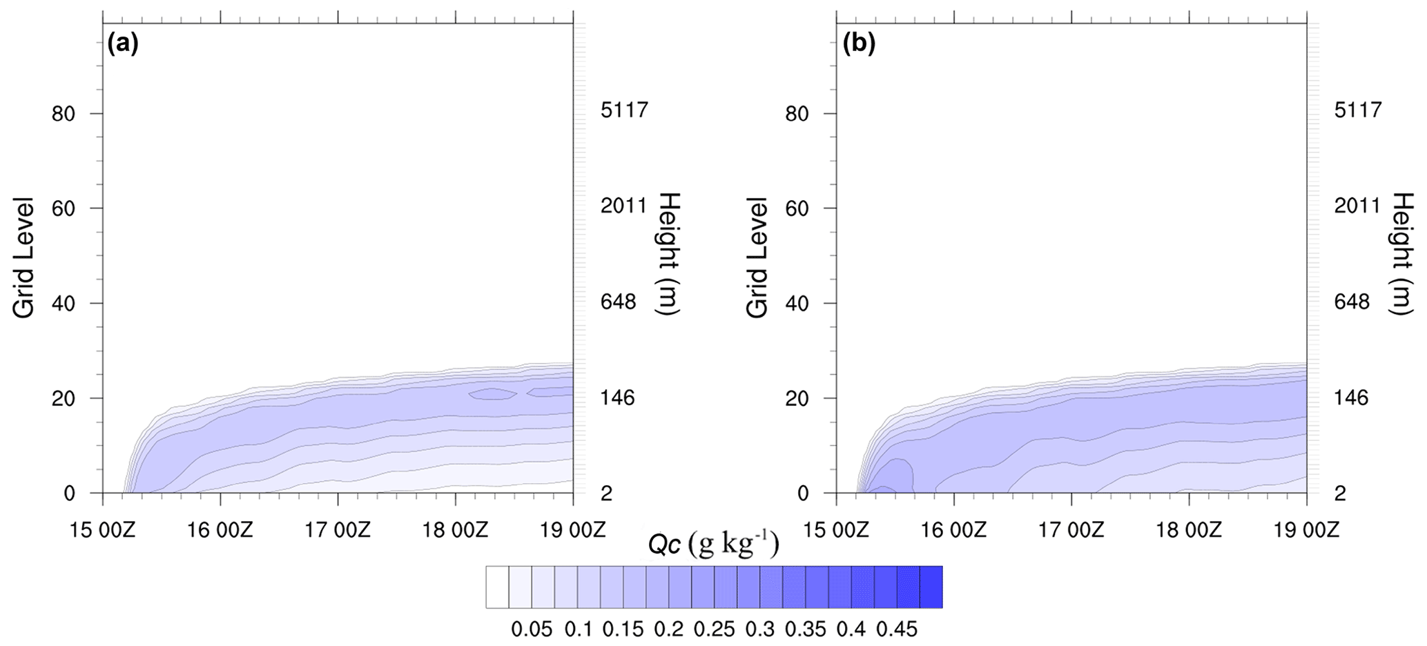
Figure 1 Contours of Q_c (g kg⁻¹) generated by WRF SCM, with 6 h of surface cooling at 3 K h⁻¹. (a) MYNN boundary layer, using the turbulence deposition scheme described with z_0c=0.01 m, plus Thompson microphysics with gravitational settling. (b) Original MYNN module with gravitational settling only in Thompson microphysics. The full vertical domain is shown to indicate that no upper-level cloud formed in these cases (it did with other input). Times on the x axis are in the format DD HHZ (day, hour in UCT(Z)), with small tick marks 4 h apart. The run start time was 15:00 Z.

Figure 1 shows contours of Q_c (g kg⁻¹) as it varies with (t; eta grid level) from the model calculations over 4 d starting, somewhat arbitrarily, at 00:00 Z on day 15 of a month (15:00 Z) so that cooling runs to 15:06 Z. Some height levels are marked to indicate the grid stretching in z. These runs are for latitude 44^∘ N (Sable Island), with 101 eta grid levels. The WRF model operates with a sigma-type vertical coordinate (η), decreasing from 1 at the lower boundary to 0 at the upper boundary, where p=p_t. It has a simple form over a flat surface. Details are in Skamarock et al. (2021). Our model grid points are not uniformly spaced in η, and the spacing increases smoothly with increasing height (decreasing η). We set p_t≈22 000 Pa to give a top boundary at about 12 km. The eta levels start at η=1 (the surface), decreasing to η=0 and p=p_t at eta level 101 (our SCM model top). In full 3-D runs, we take p_t=5000 Pa. The grid is staggered so that variables like θ, Q_v, Q_c, U and V, where θ is potential temperature, and Q_v is the water vapour mixing ratio, are at mid-levels, while the lower boundary (z=0) is at the base of the lowest grid cell. Our grid levels start with the center of the lowest cell (0) and increase upwards. In Fig. 1a, z_0c=0.01 m, while Fig. 1b is for results with the original MYNN scheme with no surface deposition, except for gravitational settling in the Thompson microphysics. Fog forms as a result of the surface cooling and extends from the surface to around eta level 20, which corresponds to z≈150 m. We were initially concerned by the wave-like features in the contour lines. These have a period of around 17 h and arise because of inertial oscillations (of period $\mathrm{2}\mathit{\pi }/f$) in the wind field, (U,V), as it adjusts to the cooling of the surface and changing turbulent momentum transfers. They decay slowly as the wind profile adjusts to the cooler surface. Values of Q_c are lower in Fig. 1a because of turbulent deposition to the surface. Figure 2 shows Q_c profiles with the MYNN boundary layer, at 16:00 Z, 24 h after the start of the model calculations and 18 h after the end of surface cooling. The additional turbulent deposition can play an important role in lowering Q_c levels in the boundary layer while, in this case, not having a significant impact above 100 m. The amount of the reduction depends on the value chosen for z_0c.

Figure 2 Q_c profiles, 24 h after the start of the integration and 18 h after the end of the surface cooling, by 18 K. Results are shown with the original MYNN (gravitational settling in Thompson microphysics only) and with a range of z_0c values (in meters). A time step, dt, of 60 s was used with 101 eta levels.

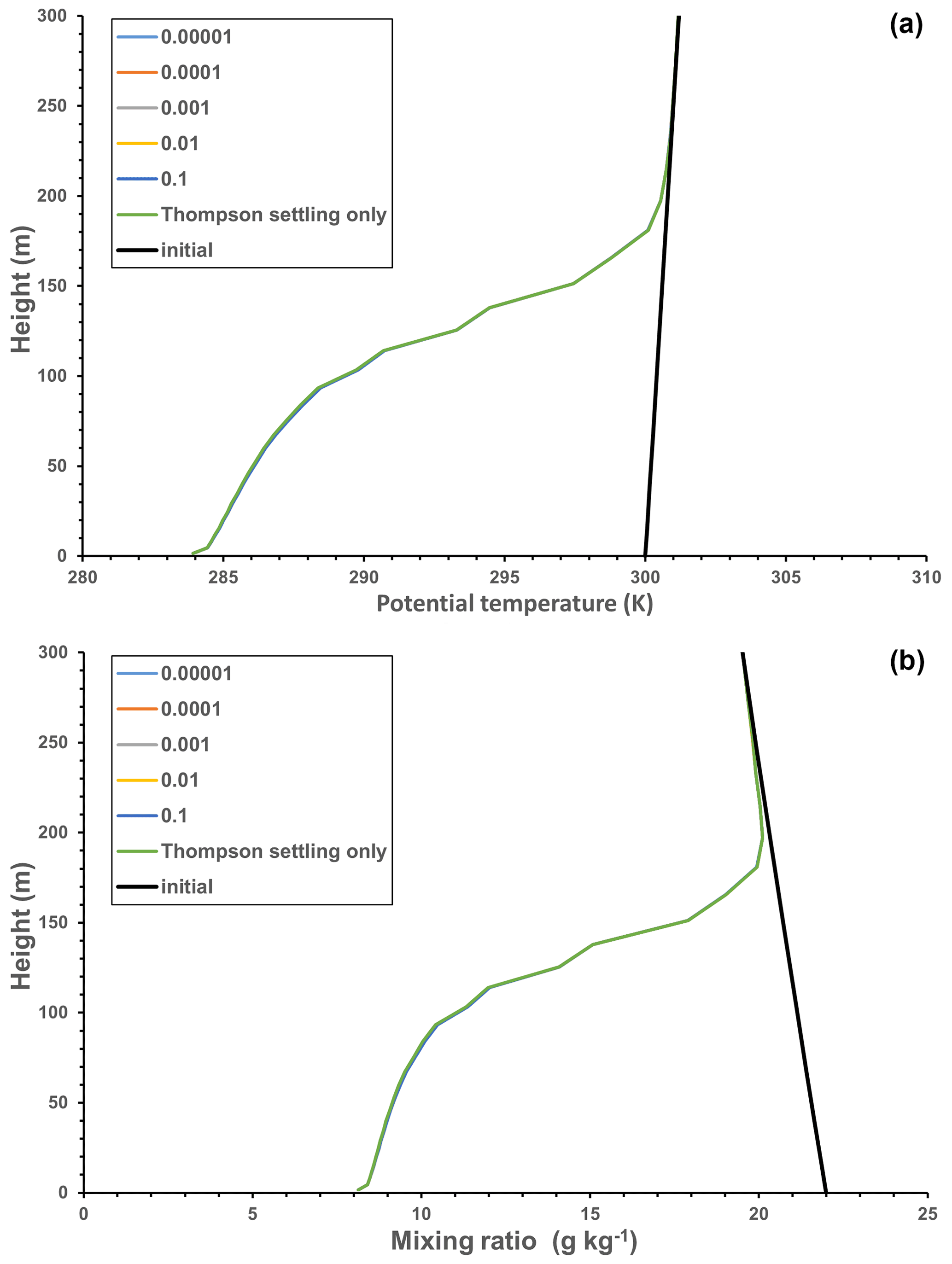
Figure 3 (a) Potential temperature (θ) and (b) Q_v profiles corresponding to Fig. 2, including the initial profiles. Note that the z_0c deposition of cloud droplets has minimal impact, and all curves are overlain.

It is interesting to note that the removal of Q_c at the lower boundary has minimal impact on the predicted temperature and water vapour, Q_v, profiles (Fig. 3). It could, however, be important when fog starts to evaporate if the air temperature rises. Note that, in generating these results, we have not included radiation (shortwave or longwave) effects in order to focus on the impacts of turbulent deposition at the water surface. Radiation can play a significant role once fog has formed, and in particular, longwave radiational cooling at the fog top (Yang and Gao, 2020) can add to the cooling rate and can enhance turbulent mixing in the upper part of the fog layer. The center of the lowest grid layer is at 1.7 m. Noting the kinks in the profiles at the lowest level in profiles of Q_c, Q_v and θ, we investigated possible causes and plotted them on an expanded height scale (not shown). They arise because in WRF modules sf_mynn and sf_fogdes the fluxes to the surface are computed with deposition velocities involving $\ln \left(\right(z+z_{\mathrm{0}})/z_{\mathrm{0}})$, while the eddy diffusivities used to compute fluxes at the top of the first level and levels above are based on length scales proportional to kz without the z₀ addition. This will not be significant for z≫z₀, but with the lowest computational levels close to the surface this could be modified. This is an internal WRF issue, noted in comments within the module_bl_mynn code.

A further point from Fig. 3b is that, with our near-saturated initial profile and strong cooling, there is a significant reduction in Q_v, of order 10 g kg⁻¹, throughout the lowest 100 m. This will be converted to Q_c, but after 24 h, most will have been deposited to surface through both gravitational settling, as in the original curves in Fig. 2, or by a combination of gravitational settling and turbulent deposition to the water surface, as in the other cases shown in Fig. 2. In runs with gravitational settling turned off in the microphysics and no turbulent deposition, the Q_c values increase significantly, to around 6 g kg⁻¹, near the surface after 12 h. This is not shown for this case, but see the 3-D case in Fig. 4b, although then there is less cooling. Gravitation settling generally prevents very high Q_c values from occurring, but additional turbulence-induced deposition further limits them.

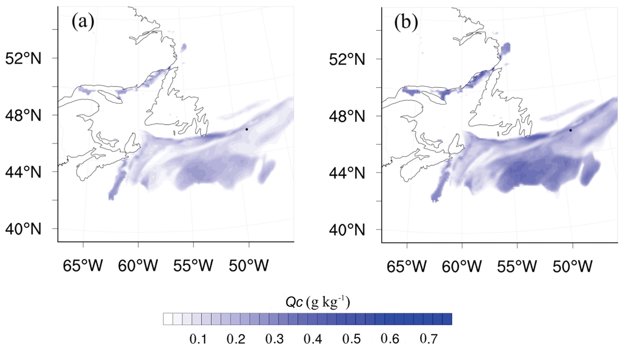
Figure 4 The 2-D fog plots at lowest model level on 1 July 2018, 18:00 Z, from WRF. Thompson microphysics with gravitational deposition (a) with z_0c=0.01 m and no turbulent deposition (b) is related to Fig. 5a. The black dot shows the point on the Grand Banks to which the profiles in Fig. 5 correspond.

7 3-D test cases

Turning to the 3-D WRF model, we have been running the model for North Atlantic simulations for summer 2018 on a domain extending from eastern Canada out beyond the Grand Banks and including Sable Island. A separate paper on comparisons with visibility measurements on Sable Island is in preparation, while some sample results are in Cheng et al. (2021). These 3-D runs have no additional surface cooling and are simply run as hindcasts of the actual situation with initial and boundary conditions taken from NCEP analyses. The sea surface temperatures are held fixed for daily 36 h runs, generally with a 12 h spin up. Note that the input initial and boundary fields had zero Q_c. They are run with hybrid_opt=0, and in the vertical direction we have a straight sigma coordinate as follows:

$$\begin{array}{}\text{(9)}& \mathit{\eta }=(p_{\mathrm{d}}-p_{\mathrm{s}})/(p_{\mathrm{t}}-p_{\mathrm{s}}),\end{array}$$

with p_t=5000 Pa. Runs were also made with hybrid opt = 2, and Q_c results were almost identical. Solar and longwave radiation can use either Goddard or RRTMG (Rapid Radiative Transfer Model for Global models) scheme, and we used the MYNN PBL (planetary boundary layer) scheme with either the Thompson or the WSM6 microphysics options. For details of these options, see Skamarock et al. (2021). Figures 4 and 5 show sample results from 6 h after the start of a run with the full 3-D model, using Thompson microphysics and Goddard radiation and long- and shortwave.

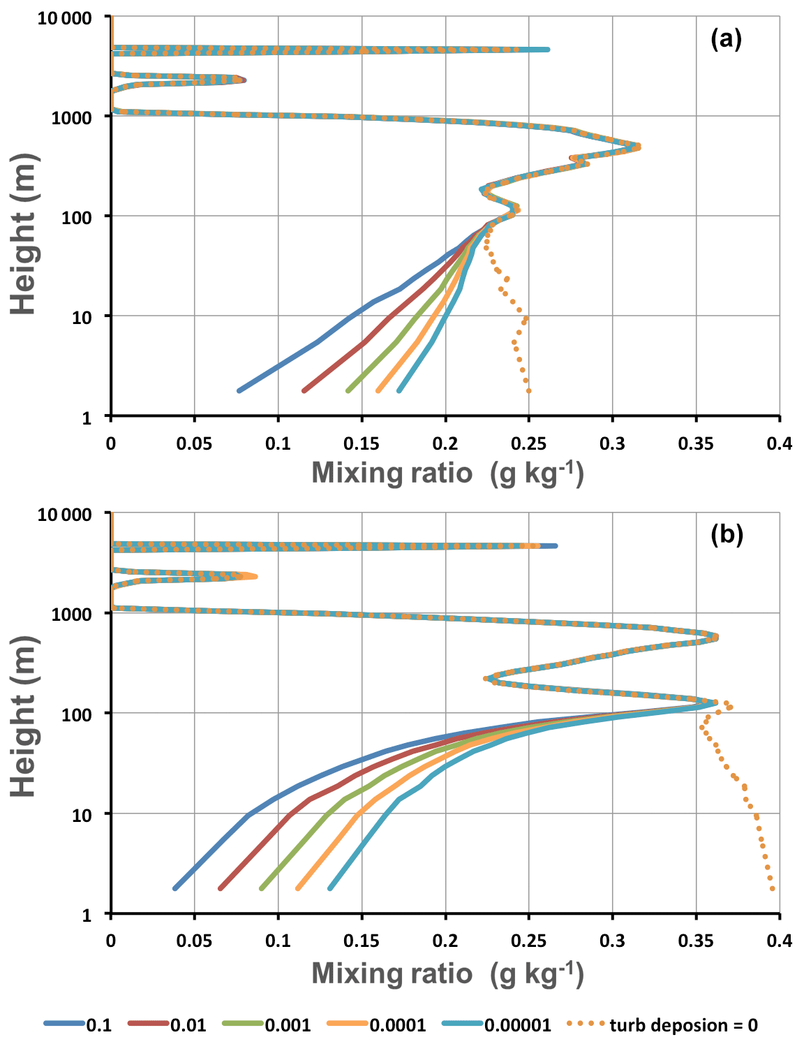
Figure 5 Sample 3-D WRF output at a fixed location over the Grand Banks, with different z_0c values (given in meters) in Q_c turbulent deposition, (a) with and (b) without gravitational settling. Start time (day, month, year, and hour) was 7 January 2018 12:00 Z, and results are for 7 January 2018, 18:00 Z. Results are with the MYNN boundary layer and Thompson microphysics.

With 3-D WRF simulations, we initially look at plots and animations over our d02 domain (see Supplement) at the lowest model level. Figure 4 is an example of 2-D plots of Q_c at the same time as in Fig. 5, with and without turbulent deposition. The black dot identifies the Grand Banks location (GB) used in Fig. 5. The value of z_0c was 0.01 m. In additional runs (not shown) with no gravitational settling, the spatial fog patterns are similar, but in the extreme case with no turbulent deposition, the Q_c values are up to 0.8 g kg⁻¹ in some areas, although it is only 0.4 g kg⁻¹ at our GB location.

In Fig. 5, the Q_c profiles show a similar response to the SCM (Fig. 2) when turbulent deposition of cloud water to the surface is introduced. Figure 5a shows a normal run, with the Thompson microphysics module accounting for gravitational settling effects. MYNN has turbulent deposition to the surface but no gravitational settling (grav_settling=0). In Fig. 5b, we removed gravitational settling from the Thompson microphysics scheme (av_c=0) and from MYNN. With no turbulent deposition to the surface, and in one special case with no gravitational settling either, there are higher Q_c values as expected. These 3-D runs used NCEP analyses as initial conditions, but the initial Q_c was set to zero everywhere. In fog, the analysis would give 100 % RH, and the model then generated Q_c within a few hours but without the strong temperature and Q_v drops that were simulated in our SCM tests. Gravitational settling (Fig. 5a) has reduced the peak Q_c values at around 100 and 900 m from the case with no settling, and the Q_c removed from those levels has settled and mixed downwards to increase the Q_c values near the ground.

Additional 3-D runs were made with the standard MYNN codes and the Katata scheme using modified deposition velocities in the other case. These matched our results obtained with a modified MYNN code. Also, in place of the Thompson microphysics scheme, we ran tests with WSM6 microphysics. In all cases, there was a large impact of turbulent surface deposition of Q_c in the lowest 100 m, even with very low values for z_0c. As an initial guide, we suggest using z_0c=0.01 m or 0.001 m as a modest value which has a solid impact. We should also emphasize that gravitational settling also has an impact on Q_c values near the surface, and both processes need to be included in models.

8 Visibility considerations

Models can predict liquid water mixing ratios, but the critical forecast issue is visibility, which will depend on the number and size distribution of the fog droplets. In dense marine fog (LWC>0.05 g m⁻³), Isaac et al. (2020; Fig. 12) show that the size distribution of marine fog droplets is generally broad and frequently bimodal, raising concerns about all simple diagnostic schemes. Despite such concerns, models such as the one proposed by Isaac et al. (2020) assume that visibility is proportional to ${\text{LWC}}^{-\mathrm{2}/\mathrm{3}}\times N^{-\mathrm{1}/\mathrm{3}}$, where N is the droplet number density (cubic meters; hereafter m⁻³). Some models include dynamic equations for N, while others assume prescribed values, typically N=10⁸ m⁻³. If the size distribution was well known and universal, then this could work, but as Isaac et al. (2020) note, the size distribution in fog over the ocean can be bimodal, and the number density can vary widely. In conditions with LWC>0.005 g m⁻³, the number density reported by Isaac et al. (2020) over a site in the Grand Banks area varies between 10⁷ and 3×10⁸ m⁻³. Medians were close to $N=\mathrm{0.8}\times {\mathrm{10}}^{\mathrm{8}}$ m⁻³. Note, however, that these measurements were at a height of 69 m above the ocean surface, and if the water surface is a sink for cloud droplets, then one would expect lower values, and maybe a different size distribution, at the World Meteorological Organization (WMO) standard visibility measurement height of 2.5 m (WMO, 2020). Chen et al. (2020) note problems with visibility that is too low from their WRF calculations coupled to the Kunkel (1984) visibility equation ($\text{vis}=-\ln \left(\mathit{\epsilon }\right)/\mathit{\beta }$ with the extinction coefficient (in kilometers; hereafter km⁻¹), β=144.7W^0.88, where W (or LWC) is in g m⁻³). The contrast threshold, ε was given as 0.02 by Kunkel (1984) but is set to 0.05, as recommended by the WMO (Boudala et al., 2012; Chen et al., 2020). In the NASA Global Systems Division (GSD) algorithm used in NCEP's Unified Post Processor version 2.2, the Kunkel (1984) result is used with ε=0.02 for visibility reductions in clouds, plus additional effects of aerosol, rainfall and humidity. The relationship between visibility and LWC can vary in these models between a power of $-\mathrm{2}/\mathrm{3}$, through −0.88 to −1 if N were proportional to LWC, but all show that too high a value of LWC or Q_c will lead to too much reduction in visibility. Running standard versions of WRF, one can compute visibilities with either the Isaac et al. (2020) equations or the GSD algorithm used in NCEP's Unified Post Processor version 2.2 (for details, see Lin et al., 2017). Both led to significantly lower values of visibility than were reported on Sable Island. Typical WRF values being of order one-tenth to one-fifth of the reported visibility, suggesting Q_c values that may be high by a factor between 5 and 30. Visibility–cloud water relationships are open to revision, with different values of ε and noting the scatter in Isaac et al.'s (2020) data, but there is a strong suggestion that WRF values of Q_c are too high without adding additional Q_c deposition.

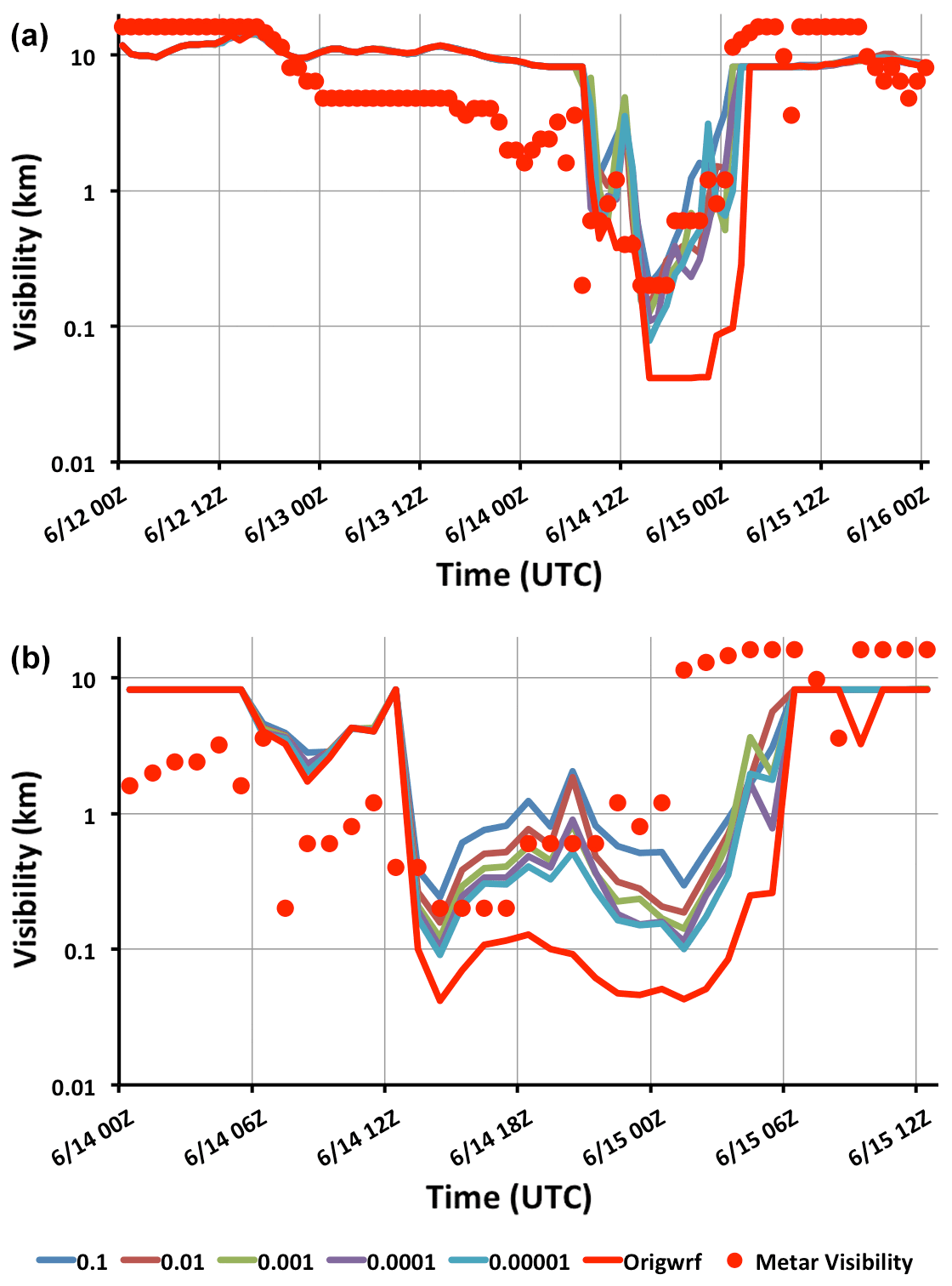
Figure 6 Sample June 2018 GSD visibility hindcasts for Sable Island at 2 m, using MYNN boundary layer and WSM6 microphysics, with different z_0c values (in meters).

Figure 6 shows sample visibility time series computed from 3-D WRF Q_c output for the Sable Island location, vertically interpolated to z=2 m, for two 36 h periods in 2018 when fog was reported at Sable Island. We should, however, note that these computations were made with a 10 km horizontal mesh, and there was no island. In reality, the presence of a land surface can modify the temperature, up or down, leading to relative humidity, LWC and visibility adjustments as air travels in from the shoreline (see, for example, Cheng, 2021). In these cases, the fog occurred in daytime, and Q_c could be lower at the weather station than offshore. Original WRF runs with just gravitational settling show seriously limited visibility (<100 m) on some occasions when METAR visibility was closer to 1 km, while, with added turbulent Q_c deposition and a range of z_0c values, the optical range was a better match to the observations. These are sample cases and a more extensive comparison is planned.

9 Conclusions

It has been known for many years that fog water can be deposited on vegetation, and this has been incorporated into some boundary layer fog models. It is also known that µm size aerosols can be removed from the atmosphere by turbulence at water, and other, surfaces (Farmer et al., 2021). It then seems surprising that, for marine fog, turbulence-induced cloud–fog droplet deposition to water surfaces has not been recognized by most modellers as a significant potential addition to the deposition associated with gravitational settling. Neglecting this can then lead to fog liquid water mixing ratios being too high and visibility forecasts being too low. This applies to specialized boundary layer models and to numerical weather prediction models. Many authors have noted the difficulties and complexity of modelling fog and accurately forecasting visibility. Making everything right will be extremely challenging, but, for marine fog, recognizing that a significant process is missing from many models could be a step in the right direction.

WRF-ARW is a major contribution to the atmospheric research endeavour, and the developers and maintainers of this huge, multifaceted, publicly available model deserve huge credit. As with anything of this size and complexity, developed and modified over many years by many individuals, it can be very hard for new users to trace through the source codes and understand just how they work. Some module codes are well documented and commented on; others are less so. Running the model is made relatively easy, and it is designed to be robust. We have done our best to understand some details and ensure that our modifications, briefly explained in the Supplement, do what we expect, but we make no guarantees.

Recent fog field programs, including LANFEX (Price et al., 2018) in the UK, SoFog 3-D (https://www.umr-cnrm.fr/spip.php?article1086&lang=fr{#}outil_sommaire_0, last access: 2 October 2021) in France and studies in India and China, have focused on fog over land but are providing valuable field data for model comparisons. The C-Fog campaign (Fernando et al., 2021) is providing valuable data on coastal fog, and the 2021–2026 Fatima (Fog and Turbulence Interactions in the Marine Atmosphere; https://efmlab.nd.edu/research/Fatima/, last access: 2 October 2021) project will be a major contribution to the understanding of marine fog.

Based on our modelling of marine fog with WRF, and reviews of the treatment of boundary layer fog in WRF and other models, it seems that a better understanding of fog droplet interaction with the ocean surface, and other surfaces, is needed. Laboratory studies might be possible, and numerical simulations may be done, but with some good in situ profile measurements through fog layers over land and water, one could start to better understand and parameterize this process. Any foggy location on land could work, but Sable Island would offer an ideal location for such a study in marine fog. It is a 43 km long, narrow (mostly <2 km wide) sand bar in the Atlantic Ocean about 175 km offshore from Nova Scotia, Canada, and will be field site during Fatima in summer 2022. Sable Island has some vegetation, cranberry bushes and grass, wild horses and many seals and is now a national park. Observations (https://climate.weather.gc.ca/climate_normals/index_e.html, last access: 3 October 2021) show more than 200 h (out of 720 h) of fog (visibility <1 km) on Sable Island in the months of June and July. An upper air station (CWSA, 71600) was operated there by Environment Canada until August 2019. Taylor et al. (1993) made winter storm measurements from the island as a part of the Canadian Atlantic Storms Program. The western tip of the island would be an ideal location for a tall mast or other profiling measurements with a variety of fog-related and standard meteorological research instrumentation at multiple levels.