the Creative Commons Attribution 4.0 License.
the Creative Commons Attribution 4.0 License.
 | 04 Oct 2021
Aerosol properties and aerosol–radiation interactions in clear-sky conditions over Germany
Anja Hünerbein
Florian Filipitsch
Stefan Wacker
Stefanie Meilinger
Hartwig Deneke
The clear-sky radiative effect of aerosol–radiation interactions is of relevance for our understanding of the climate system. The influence of aerosol on the surface energy budget is of high interest for the renewable energy sector. In this study, the radiative effect is investigated in particular with respect to seasonal and regional variations for the region of Germany and the year 2015 at the surface and top of atmosphere using two complementary approaches.
First, an ensemble of clear-sky models which explicitly consider aerosols is utilized to retrieve the aerosol optical depth and the surface direct radiative effect of aerosols by means of a clear-sky fitting technique. For this, short-wave broadband irradiance measurements in the absence of clouds are used as a basis. A clear-sky detection algorithm is used to identify cloud-free observations. Considered are measurements of the short-wave broadband global and diffuse horizontal irradiance with shaded and unshaded pyranometers at 25 stations across Germany within the observational network of the German Weather Service (DWD). The clear-sky models used are the Modified MAC model (MMAC), the Meteorological Radiation Model (MRM) v6.1, the Meteorological–Statistical solar radiation model (METSTAT), the European Solar Radiation Atlas (ESRA), Heliosat-1, the Center for Environment and Man solar radiation model (CEM), and the simplified Solis model. The definition of aerosol and atmospheric characteristics of the models are examined in detail for their suitability for this approach.
Second, the radiative effect is estimated using explicit radiative transfer simulations with inputs on the meteorological state of the atmosphere, trace gases and aerosol from the Copernicus Atmosphere Monitoring Service (CAMS) reanalysis. The aerosol optical properties (aerosol optical depth, Ångström exponent, single scattering albedo and asymmetry parameter) are first evaluated with AERONET direct sun and inversion products. The largest inconsistency is found for the aerosol absorption, which is overestimated by about 0.03 or about 30 % by the CAMS reanalysis. Compared to the DWD observational network, the simulated global, direct and diffuse irradiances show reasonable agreement within the measurement uncertainty. The radiative kernel method is used to estimate the resulting uncertainty and bias of the simulated direct radiative effect. The uncertainty is estimated to −1.5 ± 7.7 and 0.6 ± 3.5 W m−2 at the surface and top of atmosphere, respectively, while the annual-mean biases at the surface, top of atmosphere and total atmosphere are −10.6, −6.5 and 4.1 W m−2, respectively.
The retrieval of the aerosol radiative effect with the clear-sky models shows a high level of agreement with the radiative transfer simulations, with an RMSE of 5.8 W m−2 and a correlation of 0.75. The annual mean of the REari at the surface for the 25 DWD stations shows a value of −12.8 ± 5 W m−2 as the average over the clear-sky models, compared to −11 W m−2 from the radiative transfer simulations. Since all models assume a fixed aerosol characterization, the annual cycle of the aerosol radiation effect cannot be reproduced. Out of this set of clear-sky models, the largest level of agreement is shown by the ESRA and MRM v6.1 models.
- Article
(15067 KB) - Full-text XML
- BibTeX
- EndNote


Aerosols influence the earth's climate through their interaction with atmospheric radiation. A fundamental measure of the strength of this interaction is the radiative effect resulting from aerosol–radiation interactions (REari), which is also referred to as the direct radiative effect of aerosols (Boucher et al., 2014). This includes aerosols from natural and anthropogenic sources. The REari is computed as the hypothetical difference of the net irradiance with aerosols and in pristine conditions and can be considered at any vertical level of the atmosphere. Climatological studies are often focused on the REari on the total atmosphere to investigate the heating or cooling by aerosols. This requires the knowledge of the REari at the top of the atmosphere and surface. The best estimate of the global mean REari by anthropogenic aerosols, called the aerosol radiative forcing, is −0.45 ± 0.5 W m−2 at the top of the atmosphere according to the latest IPCC report and is one of the major uncertainties for estimating the total radiative forcing by anthropogenic aerosols of the climate system (Myhre et al., 2014). The REari is considered in terms of short-wave (solar) and long-wave (terrestrial) radiation, with solar and terrestrial radiation being defined as the electromagnetic radiation at wavelengths less and more than 4 µm, respectively. The REari at the surface is also of relevance for our understanding of the climate system due to its influence on the surface energy budget and thus its influence on latent and sensible heat fluxes (e.g. Chaibou et al., 2020). In addition, the effect of aerosols on the surface solar irradiance is of high interest for the renewable energy sector, e.g. the planning of photo-voltaic (PV) power plants (e.g. Schroedter-Homscheidt et al., 2013). Depending on their optical properties, aerosols reduce the global horizontal irradiance by changing both its diffuse and direct irradiance components. While the impact of REari on PV power depends mainly on changes in global irradiance, its effect on concentrating solar power is mainly caused by changes in direct irradiance. Several regional studies clearly show the impact of REari on solar power production (e.g. Gueymard and Jimenez, 2018; Neher et al., 2019), but none of them considers wavelength-dependent aerosol properties.
Considerable effort is spent over the last decades to quantify the clear-sky short-wave REari at the surface, referred to simply as REari in the following text unless indicated otherwise. The REari is studied at global (e.g. Yu et al., 2006; Bellouin et al., 2013; Kinne, 2019) and regional scales (e.g. Papadimas et al., 2012; Esteve et al., 2016; Bartók, 2016). Neher et al. (2019) found a median daily REari of 9.4 % to 14 % for six AERONET (AErosol RObotic NETwork) stations located in the region of the Economic Community of West African States (ECOWAS) using AOD retrieved from AERONET and radiative transfer calculations using libRadtran (Mayer and Kylling, 2005). For Europe, Nabat et al. (2014) quantified the REari by utilizing a coupled regional climate system model (CNRM–RCSM4). Bartók (2016) used the MAGIC radiation code with aerosols and water vapour climatology from Aerocom and ERA-Interim, respectively, for calculating REari. Esteve et al. (2016) utilized a different radiation scheme (ES96) along with aircraft measurements of aerosol optical properties during the EUCAARI-LONGREX campaign. These studies found annual-mean values of REari ranging from −7 to −15 W m−2, with uncertainties of about 5 W m−2. The discrepancies of the REari found in the literature are the result of the different methods and models used, as well as the use of a wide variety of measured data.
The present investigation is focused on REari in particular with respect to seasonal and regional variations across Germany. For this purpose, two sources of information are considered here.
First, high-quality broadband global and diffuse irradiance measurements carried out at 25 stations across Germany as part of the observational network of the German Weather Service (DWD). These observations represent the current state of the atmosphere, including aerosols. To calculate the REari, the observations are combined with different clear-sky models (CSMs) (e.g. Sun et al., 2019) to simulate the irradiance of the aerosol-free (pristine) atmosphere. A large variety of CSMs is available, ranging from simple to highly complex schemes developed for different applications. The accuracy of these models to simulate the clear-sky irradiance at the surface is intensively evaluated in numerous studies, most recently and detailed by Sun et al. (2019). CSMs are widely used to estimate the solar irradiance at the surface in cloud-free conditions. Applications range from the evaluation of power generation of photo-voltaic power plants (Bright et al., 2017) to the determination of the global radiation budget on a spatial resolution which is not possible with ground-based observations (Ruiz-Arias and Gueymard, 2018). These models can also be used in the quality control of observational data (e.g. Long and Ackerman, 2000; Ineichen, 2014; Reno and Hansen, 2016). In this study, the CSMs utilized are evaluated on their usability for REari quantification. The CSMs are namely the Modified MAC model (MMAC), the Meteorological Radiation Model (MRM) v6.1, the Meteorological–Statistical solar radiation model (METSTAT), the European Solar Radiation Atlas (ESRA), Heliosat-1, the Center for Environment and Man solar radiation model (CEM), and the simplified Solis model. With this approach, the REari is computed directly for the location of the measuring station. This makes this approach particularly suitable for case studies such as determining the influence of aerosol on the performance of photo-voltaic systems. On the other hand, the restricted temporal and spatial coverage are limitations for climate studies.
Secondly, the Copernicus Atmosphere Monitoring Service (CAMS) provides a global reanalysis (CAMS RA) dataset of atmospheric composition including aerosol properties (Inness et al., 2019a). The CAMS RA is based on the Integrated Forecast System (IFS) of the European Centre for Medium-Range Weather Forecasts (ECMWF) and the assimilation of satellite observations; the amounts of various atmospheric constituents are estimated by explicit modelling of their sources, atmospheric transport and their sinks. This dataset provides complete spatio-temporal coverage and also enables explicit radiative transfer simulation as all the required variables are included. The aerosol optical properties are highly dependent on the aerosol mixture, which in the underlying aerosol model of CAMS RA is described by a set of seven different aerosol types. Therefore, a lower accuracy of the aerosol representation can be assumed compared to locally measured reference values. Furthermore, the accurate representation of the REari at a specific location is limited by sub-grid scale effects (e.g. Gueymard and Yang, 2020). In this study, the CAMS RA aerosol representation is evaluated using the AERONET direct sun and inversion products as reference, including single scattering albedo and asymmetry parameter (e.g. Dubovik and King, 2000; Sinyuk et al., 2007). This provides insight into the possible shortcomings of the aerosol input from CAMS RA and the ability of a detailed uncertainty analysis on REari simulated using the CAMS RA data. The level of agreement between the CAMS RA aerosol optical depth (AOD) and Ångström exponent (AE) products compared to reference observations is promising and has already been extensively evaluated versus ground-based observations (e.g. Inness et al., 2019a; Witthuhn et al., 2020; Zhang et al., 2020; Gueymard and Yang, 2020). Bulk absorption properties (e.g. single scattering albedo) has, to our knowledge, not been evaluated yet, despite its major impact on REari calculation (Thorsen et al., 2020). The REari is simulated with the TROPOS (Leibniz Institute of Tropospheric Research) – Cloud and Aerosol Radiative effect Simulator (T–CARS) using the CAMS RA data as input to the offline version of the ECMWF radiation scheme (ecRad) (Hogan and Bozzo, 2018).
Given the fundamental differences of these two approaches, the consistency of the underlying aerosol properties and the resulting REari is of prime interest to us. The scheme presented in Fig. 1 outlines the analysis conducted in this study. Specific goals of the study are summarized as follows:
-
evaluation of the CAMS RA aerosol properties database versus AERONET version 3 direct sun and inversion products;
-
sensitivity analysis of REari on aerosol optical properties and atmospheric parameters;
-
investigation of the influence of aerosol and atmospheric definitions in the CSMs on the retrieval of irradiance and REari;
-
evaluation of irradiance and REari estimates, by intercomparing CSMs and the T–CARS approach and comparing with DWD irradiance observations as reference;
-
determination of aerosol conditions and best estimate of REari over Germany in the year 2015.
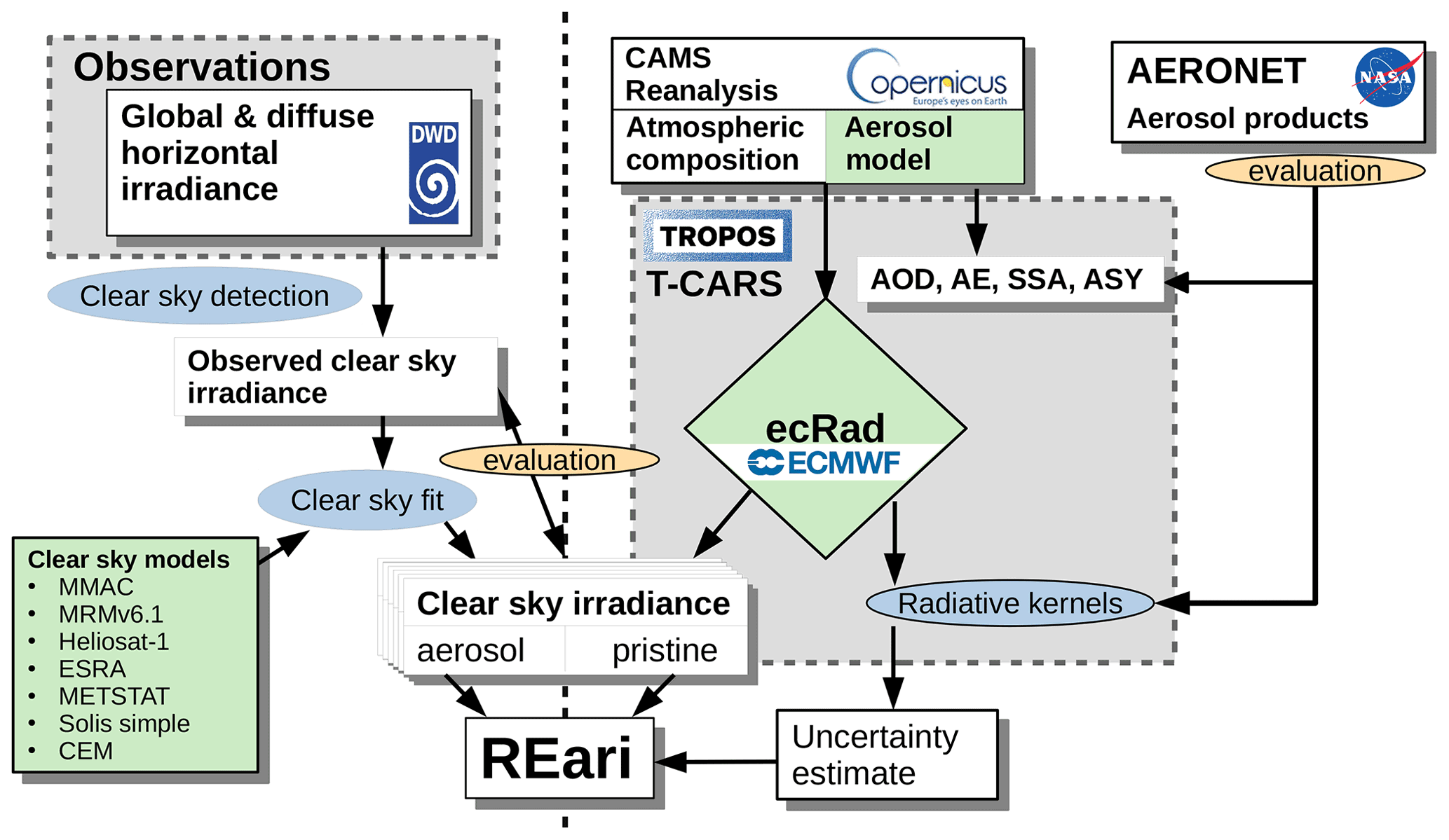
Figure 1Schematic view of the analysis conducted in this study. Datasets are shown as white boxes, methods as blue ellipses and models in green. The study involves clear-sky detection (see Sect. 3.1), clear-sky fitting (see Sect. 3.2), the T–CARS setup (see Sect. 3.3), and a method utilizing radiative kernels to analyse the sensitivity and estimate the uncertainty of the REari simulation (see Sect. 3.3.4).
This paper is structured as follows: first, the utilized datasets are described in Sect. 2. Methods and metrics used in this study are described in Sect. 3. The results and discussion are presented in Sect. 4, including uncertainty and sensitivity analysis of the T–CARS setup (Sect. 4.1), intercomparison of irradiance and REari estimates with the different setups and comparison to DWD observations (Sect. 4.2), and the best estimate of REari over Germany in 2015 (Sect. 4.3). Finally, the results are concluded in Sect. 5.
In this section, the datasets utilized for this study are described. Information on the data availability is given separately at the end of the article.
2.1 DWD radiation network
This study is based on a dataset of 1 min average values of the downwelling short-wave broadband global and diffuse horizontal irradiance observed at 25 stations in Germany during the year 2015 as part of the German Weather Service (DWD) observational network (Becker and Behrens, 2012). Global horizontal irradiance (GHI) and diffuse horizontal irradiance (DHI) is measured using secondary standard pyranometers of types CM11 and CM21 from the manufacturer Kipp & Zonen. To observe the diffuse horizontal irradiance, the pyranometers are equipped with a shadow ring to block the direct component of the incoming solar radiation. A correction is applied to the DHI to account for the diffuse radiation blocked by the shadow ring. All pyranometers are operated in a ventilation unit, which blows slightly preheated air over the radiometer dome to impede the formation and accumulation of dew, ice and snow. The direct normal irradiance (DNI) is calculated as the difference of GHI and DHI, scaled by the inverse of the cosine of the solar zenith angle. In addition, a fully automated quality control is applied to the dataset following the recommendation of the world radiation monitoring centre for BSRN data (Long and Shi, 2008; Schmithüsen et al., 2012).
The measurement uncertainty under clear-sky conditions for this class of pyranometers is about 2 % for GHI and about 4 % for DHI, due mostly to uncertainty of the shadow ring correction. Therefore, the uncertainty of DNI is estimated to be about 5 % under clear-sky conditions. The calibration of the instruments is conducted at a 2-year interval and is performed in the laboratory using a lamp and a reference pyranometer traceable to the World Radiation Reference (WRR). All stations are maintained by weather observers or technical staff to guarantee the regular cleaning of instruments and adjustment of the shadow ring manually at least once a week.
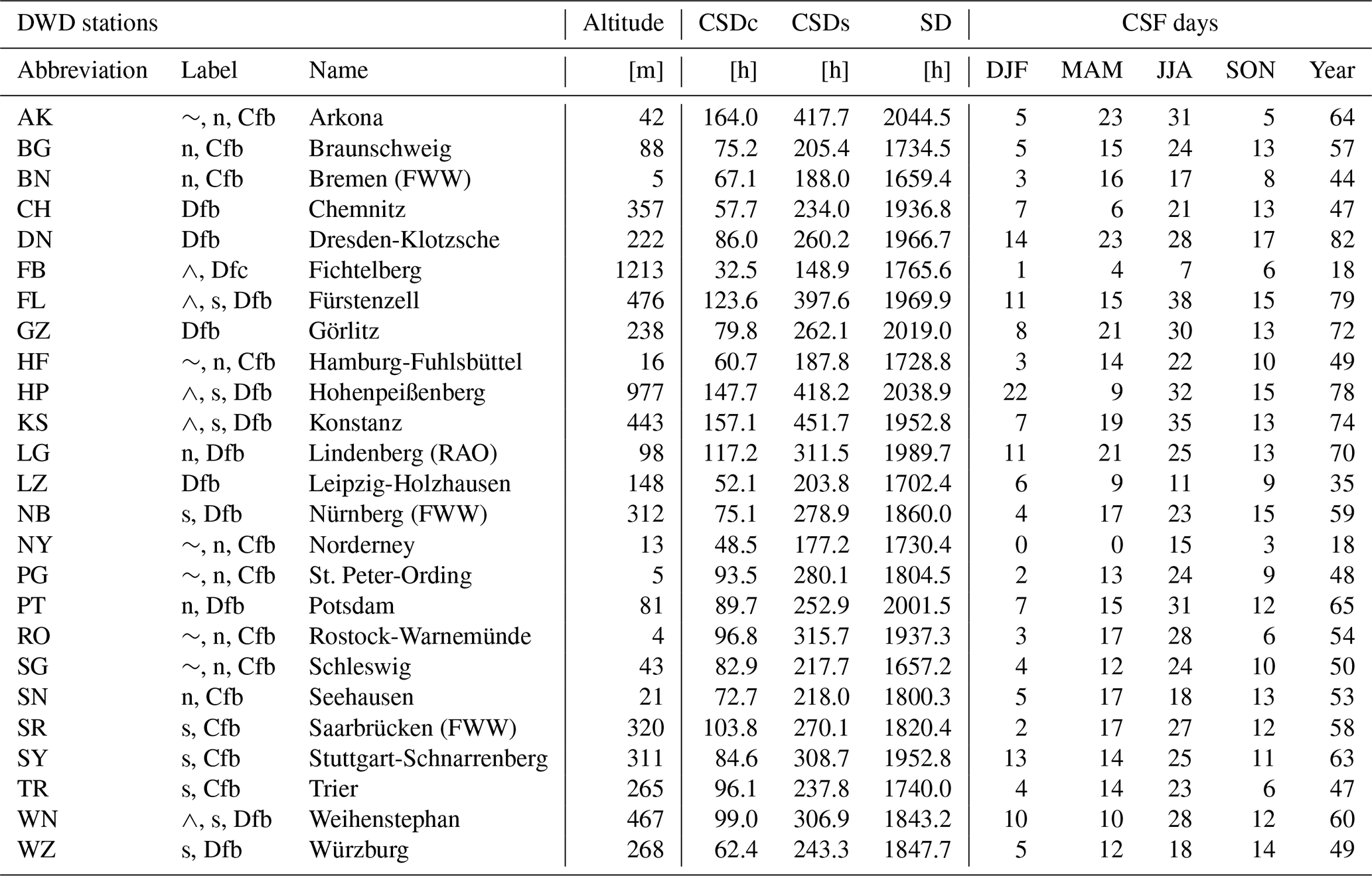
To study regional differences, the DWD stations are labelled based on their location, altitude and Köppen–Geiger climate classification (Beck et al., 2018). Measurements of stations with the same tag are aggregated in the analysis. The following classes are defined:
-
(coastal, ∼) stations in cities in coastal areas;
-
(mountain, ∧) stations with an altitude higher than 400 m;
-
(south) stations on latitudes smaller than 50∘ N;
-
(north) stations on latitudes larger than 52∘ N;
-
(Cfb) stations of temperate climate with no dry season and warm summer;
-
(Dfb) stations of cold climate with no dry season and warm summer;
-
(Dfc) stations of cold climate with no dry season and cold summer.
An overview of the station locations and labels is shown in Fig. 2 and Table 1.
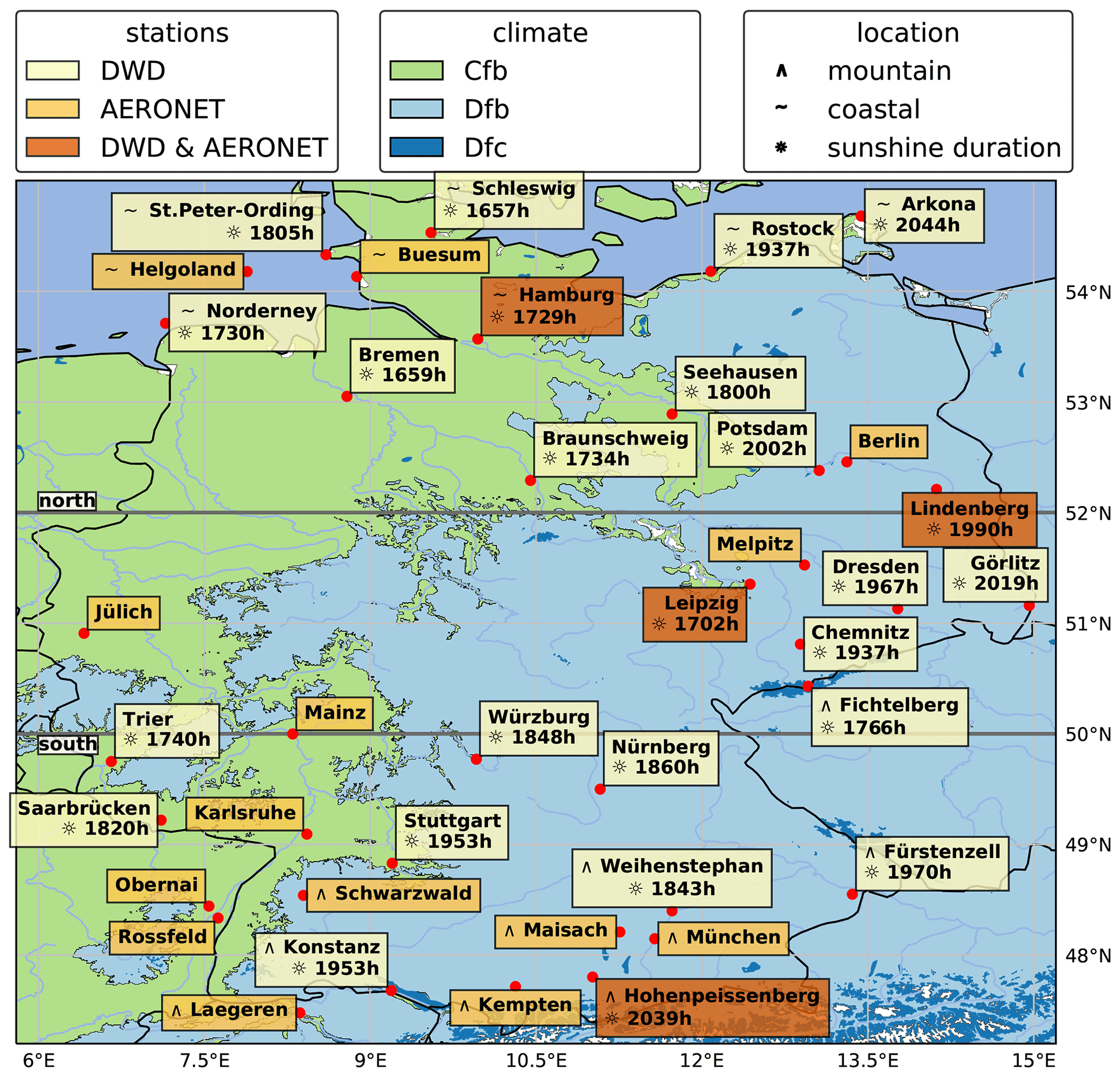
Figure 2Map of Germany showing the locations of DWD and AERONET stations. The sunshine duration is calculated from the measured irradiance data at the DWD stations and shown as accumulated hours for the year 2015. On the map, location labels are indicated for mountain, coastal, northern and southern stations. The underlying map shows the Köppen–Geiger climate classification (Beck et al., 2018).
Table 1Table of available DWD stations with corresponding altitude and selection labels. Hours of clear sky attributed to cloud-free (CSDc) and clear sun (CSDs) are shown in comparison to the WMO sunshine duration (SD). In addition, the number of days feasible for the CSF method are shown for every season and the year 2015.
2.2 CAMS reanalysis
The Copernicus Atmosphere Monitoring Service (CAMS) provides a reanalysis dataset (CAMS RA) of atmospheric composition (Inness et al., 2019a). CAMS RA is produced by the ECMWF with CY42R1 of the Integrated Forecast System (IFS) and provides global information on aerosol composition as well as various trace gases and meteorological parameters (e.g. pressure, temperature, humidity). It was developed based on the experiences gained with the former Monitoring Atmospheric Composition and Climate (MACC) reanalysis and the CAMS interim analysis (Inness et al., 2019a). Output parameters are provided at a temporal resolution of 3 h on a global grid of 0.75∘ (corresponding to a T255 spatial resolution) and for 60 vertical model levels. For a best estimate of the output parameters, CAMS RA relies on the assimilation of global satellite observations into the IFS.
Aerosol in the CAMS system is represented by five aerosol types, which are assumed to be externally mixed: sea salt, dust, organic matter, black carbon and sulfate aerosol. Hygroscopic effects are considered for organic matter, black carbon, sulfates and sea salt. Mineral dust and sea salt aerosol are described using three size bins each. The climatology used to describe the spectral aerosol optical properties in the ECMWF models is described in detail in Bozzo et al. (2020a). The spectral aerosol optical properties for each species are computed for the 30 radiative bands of the ECMWF radiative scheme (Hogan and Bozzo, 2018) as well as for 20 single spectral wavelengths in the range of 340 to 2130 nm.
In terms of aerosol properties, the AODs from the products of the MODIS C6 from both Terra and Aqua are assimilated, while the composition mixture is maintained as given from the IFS. Before its failure in March 2012, retrievals from the Advanced Along-Track Scanning Radiometer (AATSR; Popp et al., 2016) flown aboard the Envisat mission were also being assimilated. At the time of writing, the dataset covers the period 2003–2019 and will be extended into the future in the coming years.
2.3 AERONET
Global long-term ground-based measurements of aerosol optical properties are provided at numerous stations by the AERONET project (Holben et al., 1998, 2001). AERONET sites are equipped with a standardized multi-spectral sun-photometer manufactured by the company CIMEL. It measures the direct-beam irradiance at several spectral channels between 340 and 1640 nm. The AERONET direct sun algorithm provides spectral AOD and AE (Giles et al., 2019). The uncertainty of the resulting spectral AOD was intensively evaluated and is estimated to about ±0.02 for the AERONET version 3 products (Giles et al., 2019). In this study, the level 2.0 (quality assured) database is used. Furthermore, AERONET inversion products estimate spectral single scattering albedo (SSA) and the asymmetry parameter (ASY) using almucantar scans by the sun photometer (Sinyuk et al., 2007, 2020). For this study, SSA and ASY are taken from the level 1.5 (cloud-screened and quality-controlled) database. The uncertainty of these parameters has been estimated by perturbation of measurements and auxiliary inputs. For spectral SSA and for an urban or industrial area, the standard uncertainty has been estimated to about ±0.03 (Sinyuk et al., 2020), while in case of ASY and sites in Germany, the mean standard uncertainty is about ±0.01. The uncertainty estimates for SSA and ASY can be acquired from the AERONET website.
In Germany and close to the German border, a total of 25 AERONET stations are available, counting permanent and campaign-based datasets in the period from 2003 to 2019. The locations of the stations are shown in Fig. 2, except for stations of the HOPE campaign, which are located close to the permanent sites Jülich and Melpitz.
This section gives an overview of the methods and algorithms utilized in this study. The REari (ΔF) at the surface or top of the atmosphere (TOA) is computed by
where the net irradiances (down–up) are denoted as Fnet,aer (with aerosols) and Fnet,pri (without aerosols). For the total atmosphere, REari can be computed from the difference of TOA minus surface REari, indicating atmospheric heating if the result is a positive value.
Comparison analyses are focused mainly on the following metrics: standard deviation (SD), mean bias error (MBE), root-mean-square error (RMSE) and Pearson correlation coefficient (R, referred to simply as correlation in the following text).
The clear-sky detection and model algorithms as well as the offline version of the ecRad radiation scheme are publicly available; see the section on code and data availability at the end of the article.
3.1 Clear-sky detection
In this study, only clear-sky conditions are considered. Therefore, determination of the clear-sky state of the atmosphere is a critical aspect for the accuracy of our results. Here, it is determined by applying a clear-sky detection (CSD) method to the irradiance measurements of the DWD, the Bright–Sun CSD algorithm proposed by Bright et al. (2020). This method was developed based on a detailed analysis of the performance and shortcomings of numerous earlier methods in the study by Gueymard et al. (2019). The main goal of its development was to combine the best aspects of previous methods in a single, globally applicable algorithm.
Following the examples of Long and Ackerman (2000) and Reno and Hansen (2016), all three irradiance components are considered by the algorithm, and a multi-criteria approach is adopted to identify changes associated with cloudiness in the irradiance time series, respectively. Applying the unmodified Reno method (Reno and Hansen, 2016) initially to the GHI data to identify potential clear-sky periods, a first guess of GHI, DHI and DNI is subsequently optimized by scaling factors to match the observations as proposed by Alia-Martinez et al. (2016) and Ellis et al. (2018). A set of threshold tests is then applied in a tri-component analysis, based on the investigation by Gueymard et al. (2019) and as documented in Bright et al. (2020): a modified Reno method is applied to GHI and DHI, including threshold tests on the running mean, variance and extremes adapted for different solar zenith angles; for the DNI, clear-sky periods are identified by comparing the ratio of the observed DNI to the clear-sky DNI using a dynamic threshold depending on the sun elevation, inspired by Long and Ackerman (2000), Quesada-Ruiz et al. (2015), and Larrañeta et al. (2017).
Two types of situations can be differentiated: the “cloudless-sky” method involves duration criteria, which require prolonged periods of clear-sky condition within a cascade of two moving windows of 90 and 30 min length to ensure that the specific situation is not affected by cloud contamination, based on the filters defined in Shen et al. (2018). The less stringent “clear-sun” mode disables the duration filters, therefore only providing the information that the sun disk is free of clouds. Both methods have been applied to the observations in this study and are compared in Table 1.
The Bright–Sun algorithm thus requires the measured GHI and DHI as input, as well as first-guess estimates of the clear-sky GHI and DHI. From the GHI and DHI, the DNI is calculated internally. It is relatively insensitive to the accuracy of the CSM, which is used to provide the initial clear-sky irradiance estimate. Therefore, a simple CSM from Kasten (1983) (KASM) is used to calculate the clear-sky irradiance in this study. Besides the solar zenith angle, the KASM model only requires surface pressure and water vapour column as input and no information on aerosol properties. The surface pressure measured at each DWD station and the altitude-corrected water vapour column acquired from the closest station of the Global Navigation Satellite System (GNSS) meteorology product of the German Research Centre of Geoscience (GFZ) (Ning et al., 2016) are used here. Despite the limited set of inputs, the performance of the KASM model is ranked on place 16 in a comparison of 75 CSMs for observations in temperate climate in the study of Sun et al. (2019). According to Sun et al. (2019), clear-sky irradiance calculated with KASM shows an MBE below 3 %, RMSE below 5 % and a correlation of 0.98 compared to measurements at ground stations across all climates.
3.2 Retrieval of AOD and REari based on clear-sky models
To retrieve the surface REari from clear-sky broadband irradiance observations, an estimate of the clear-sky irradiance without aerosols is required. For this purpose, several CSMs are used. Furthermore, the CSMs are used to fill cloud-contaminated gaps in the observation data in order to calculate appropriate daily averages of REari. This is accomplished by inverting the CSM for a daily mean AOD using a fitting method to clear-sky irradiance observations (CSF).
The following CSMs are used: MMAC, MRM v.6.1, METSTAT, ESRA, Heliosat-1, CEM and the simplified Solis model (see Appendix A for a detailed description). The models have been selected based on the ranking established by Sun et al. (2019), as well as their input requirements. The design of this analysis requires that the CSM explicitly contains AOD as an input parameter. This AOD value can be a spectral or broadband value, but models which require additional aerosol parameters have also been excluded. For these CSMs, the clear-sky irradiance without the effect of aerosols can be estimated by setting the AOD to zero. The selected CSM-required input parameters and details about the definition of aerosols and the atmosphere are given in Table 2.
Table 2The table lists the CSMs used in this study and their definitions, assumptions and considered input parameters. Parameters considered as input are marked with (i). Listed parameters are the assumed solar constant (S0) and scaling for site altitude, which is usually applied in the definition of air mass (m). In addition, the surface albedo (asfc), transmittance from Rayleigh scattering (TR), considered ozone column (O3) and transmittance from absorption by mixed gases in the atmosphere (TG) are listed. The aerosol representation is listed for its extinction and scattering properties to calculate the direct normal and diffuse irradiance, respectively. Some aerosol scattering functions are based on a fixed SSA (ω) value. All models receive measured pressure (p) and water vapour column as input. In all models, a standard pressure (p0) of 1013.25 hPa is assumed.
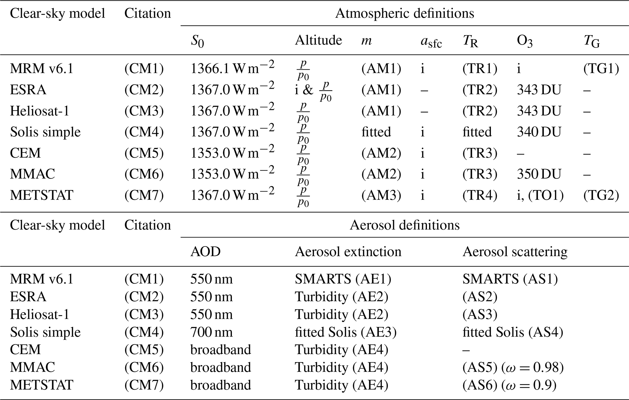
(CM1) Kambezidis et al. (2017); (CM2) Rigollier et al. (2000); (CM3) Hammer et al. (2003); (CM4) Ineichen (2008a); (CM5) Atwater and Ball (1978); (CM6) Gueymard (2003); (CM7) Maxwell (1998). (AM1) Kasten and Young (1989); (AM2) Hammer et al. (2003); (AM3) Kasten (1965). (TR1) Psiloglou et al. (1995); (TR2) Kasten (1996); (TR3) Hammer et al. (2003); (TR4) Bird and Hulstrom (1981). (TO1) Heuklon (1979). (TG1) Psiloglou and Kambezidis (2007); (TG2) Bird and Hulstrom (1981). (AE1) Kambezidis et al. (2017); (AE2) Ineichen (2008b); (AE3) Ineichen (2008a); (AE4) Unsworth and Monteith (1972). (AS1) Kambezidis et al. (2017); (AS2) Rigollier et al. (2000); (AS3) Dumortier (1995); (AS4) Ineichen (2008a); (AS5) Davies and McKay (1982); (AS6) Bird and Hulstrom (1981).
A mandatory step for the CSF is to determine the clear-sky state of the recent measurement. In this study, the CSF is used in combination with the cloudless-sky CSD. In the further text, a situation identified as cloudless sky is simply called clear sky (see Sect. 3.1).
An observation day is considered for CSF if the identified clear-sky situations are spread at least over 2 h during the day. This ensures different solar zenith angles as support centres for the fit. The number of days sufficient for CSF using our criterion are listed in Table 1. The threshold of 2 h is a somewhat arbitrary choice. Stricter thresholds lead to an increased fit performance but dramatically reduce the available amount of data. Analysis of simulated clear-sky irradiance accuracy fitted with different thresholds (not shown here) shows that this choice leads to a considerable balance of fit performance and data quantity.
Fulfilling this requirement, each of the selected CSM is compared to the irradiance observations at the identified clear-sky situations. The agreement between the CSM and observation is determined by a set of statistical metrics following Gueymard (2014). The following metrics are considered: standard deviation (SD), root-mean-square error (RMSE), the slope of the best-fit line, the uncertainty at 95 % and the t statistic. These metrics are indicators of dispersion between the observation and prediction. Each of the metrics indicates the best agreement if its value is zero. The free AOD variable is varied until the sum of all metrics is minimal. This approach implies a fixed AOD value through the day. The so inverted AOD value is limited to physical values in the range from 0 to 0.7 and then used to calculate the clear-sky irradiance with the CSM for the full day and fill the cloud-contaminated gaps in the irradiance observation.
For the retrieval of REari from this approach, the net flux with aerosol is fitted as described above. For the irradiance in pristine conditions, the AOD input value for the CSMs is zero. The utilized CSMs are developed and evaluated to represent the clear-sky irradiance in the presence of aerosols (Sun et al., 2019). Setting AOD to zero in these models may lead to large uncertainties. Furthermore, additional data of surface albedo are required to calculate the upwelling radiation. The surface albedo data are acquired from the EUMETSAT Satellite Application Facility on Land Surface Analysis (LSA SAF; Trigo et al., 2011). The 1 min temporal resolution of the observational approach is feasible for the calculation of the daily average of REari, without the need of an up-sampling process.
3.3 Radiative transfer simulations
The TROPOS – Cloud and Aerosol Radiative effect Simulator (T–CARS) is a Python-based framework for radiative transfer simulations, in particular for investigating the radiative effects of clouds and aerosols, which has been extended and used for the present study. T–CARS has been developed within the TROPOS Remote Sensing department (Barlakas et al., 2020).
Based on various supported input data sources describing the meteorological state of the atmosphere, aerosol and cloud properties, and trace gases, T–CARS can simulate the resulting vertical profiles of broadband irradiances and heating rates as output. For this study, the CAMS RA (Sect. 2.2) is used as input, and required input variables have been retrieved from the Copernicus Atmosphere Data Store. In the present study, the radiative transfer equation is solved using the ecRad radiation scheme (Hogan and Bozzo, 2018), and cloud effects are not considered.
As CAMS RA provides aerosol properties in the form of vertical profiles of the mass mixing ratio for each considered aerosol type, conversion routines for calculating the resulting aerosol optical properties have been created and are described here. In addition, the precise method used to simulate station time series for comparison purposes is explained, in particular the adjustment of inputs to account for the station elevation.
3.3.1 CAMS RA aerosol optical properties
In this study, four optical properties of aerosol are investigated and compared to AERONET observations. The aerosol optical depth (AOD), the Ångström exponent (AE), the single scattering albedo (SSA) and the asymmetry parameter (ASY). Each property describes a different aspect of the interaction of aerosols with radiation. The AOD is a measure of extinction of radiation by aerosols, the AE describes the spectral dependency of AOD, the SSA is the fraction of scattering to absorption of radiation by aerosols, and ASY describes in which direction radiation is mainly scattered.
The column-integrated values of AOD, AE, SSA and ASY are calculated from model level CAMS RA mass mixing ratios using the aerosol optical properties database described by Bozzo et al. (2020b) as shown in Appendix B. For better comparability with AERONET products, the column-integrated aerosol optical properties are calculated for a reference wavelength of 550 nm, using linear interpolation in wavelength. The AE(α) is calculated using the AOD at 440 and 870 nm with the Ångström relation:
To evaluate the method described above, the spectral AOD at wavelengths 469, 550, 670, 865 and 1240 nm is compared to the AOD product provided by CAMS RA. The comparison shows a high level of agreement as shown in Table D1. Therefore, the aerosol properties calculated with T–CARS are used to represent the CAMS RA aerosol properties database in the evaluation versus the AERONET direct sun and inversion products (Sect. 4.1.1).
3.3.2 Collocation to measurement stations
In order to evaluate the 3-hourly, gridded CAMS RA dataset to measurements conducted at a fixed location, we use the following collocation strategy:
For the evaluation of the CAMS RA aerosol properties (see Sect. 4.1.1), the AERONET dataset is interpolated in time with the nearest- neighbour method using a maximal distance of 90 min to ensure no interference by changing atmospheric and aerosol conditions and ensure comparability of the CAMS RA and AERONET dataset. Next, a subset of the CAMS RA data is calculated for each station coordinate by a bilinear interpolation in space. As the CAMS RA resolution is 0.75∘, the measurement from the observing station might not be representative for the whole grid cell, especially in the case of orographic inhomogeneity as aerosols tend to be concentrated near the surface. Therefore, the measured surface pressure or altitude at the station is used to scale the CAMS RA model level pressure instead of the surface pressure of the CAMS RA dataset. This ensures comparability to the measurement station and is especially needed in regions with highly variable orography (e.g. high-altitude sites). Note that this approach is different of using a scale-height correction for AOD only (e.g. Bright and Gueymard, 2019), as AOD, AE, SSA, ASY and the clear-sky irradiance are compared to ground-based observations in this study.
For the evaluation of REari quantification from the observational approach, an interpolation in time is not necessary as daily averages are used for the comparison (see Sect. 4.2.3). Instead, the temporal resolution of the CAMS RA input data is enhanced to 30 min by linear interpolation of each parameter. The original temporal resolution is 3 h, which is not sufficient for an accurate daily average. Analyses with further increased temporal resolution show that a resolution of 30 min is sufficient for REari daily average calculation (not shown here).
For the comparison of surface REari from CSM-based simulations, the REari simulated with the CAMS RA input is adjusted to avoid inconsistencies of different surface albedo used for the calculations. As Eq. (1) can be reformulated at surface level using the surface albedo (αsfc) by
the adjusted CAMS RA REari (ΔF′) is calculated as follows:
where denotes the requested surface albedo of either AERONET or LSA SAF as used for CSM simulations.
3.3.3 Radiation scheme ecRad
The radiation scheme ecRad (Hogan and Bozzo, 2018) is used in the T–CARS setup to simulate clear-sky irradiance with and without aerosols at the surface and top of the atmosphere. This radiation scheme was developed for the use in the ECMWF model but is also available as a detached offline version which is used in this study. Due to its modular structure, this radiation scheme is fully compatible with the aerosol properties database from CAMS RA (Bozzo et al., 2020a). As this study is entirely focused on the clear-sky REari, the short-wave homogeneous solver Cloudless is used to solve the radiative transfer equation in ecRad. The simulation conducted with ecRad provides the up- and downwelling irradiance at every model level. Further, the direct downwelling irradiance is provided. The ecRad scheme applies the δ-Eddington scaling to solve the radiative transfer equation (Joseph et al., 1976; Hogan and Bozzo, 2018). Therefore, the DNI simulated with ecRad is systematically overestimated depending on the atmospheric and aerosol scattering properties (Sun et al., 2016; Räisänen and Lindfors, 2019). Calculations are done twice – once with and once without aerosols. From this output, the REari is calculated for the surface and top of the atmosphere.
3.3.4 Irradiance and REari kernels
The sensitivity of simulated irradiance and REari on aerosol properties and atmospheric parameters is investigated in this study. Of particular interest are the aerosol optical properties such as AOD, AE, SSA and ASY, which affect the extinction of radiation by aerosols. In addition, the sensitivity on other atmospheric parameters such as surface albedo, ozone and water vapour is investigated, due to their strong effects on the radiation budget.
For this purpose, partial derivatives (e.g. Soden et al., 2008; Shell et al., 2008; Thorsen et al., 2020) on a function f(x,…) are approximated by imposing a small perturbation δx to the variable x as follows:
Similar to the analysis of Thorsen et al. (2020), the size of the perturbation is chosen as a 1 % increase to the base value (δx=0.01x). These approximated partial derivatives will be computed for GHI, DNI, and REari and referred to as irradiance kernels and the REari kernel, respectively. As not denoted here explicitly, all kernels and variables are vertically integrated and also a function of time, latitude, longitude, wavelength bands and altitude.
In T–CARS these kernels are calculated for the parameters AOD, AE, SSA, ASY, O3 mixing ratio, H2O mixing ratio and surface albedo. The perturbation of the aerosol optical properties is done on the aerosol specification input file for ecRad for all aerosol classifications and wavelength bands simultaneously. The O3 and H2O mixing ratios are directly scaled in the ecRad radiation scheme. The surface albedo is directly perturbed in the ecRad input file. Since AOD, SSA and ASY vary spectrally, a relative broadband kernel is calculated by the sum over all wavelength bands (λ) and then scaled to 550 nm (Thorsen et al., 2020):
This relative broadband kernel provides the sensitivity to a perturbation in AOD, SSA and ASY at 550 nm. As AE, O3, H2O and surface albedo are spectrally independent, these broadband kernels are directly calculated from Eq. (5) using broadband fluxes simulated with ecRad.
The kernels are used to determine the systematic and random errors of the simulated irradiance and REari. In this study, only the errors resulting from errors in the aerosol optical properties of the CAMS RA input dataset are considered. For this purpose, the kernels are scaled with the MBE (ε) and RMSE (σR) of parameters (j) AOD, AE, SSA and ASY:
In this section, the results of the following analyses are presented: in Sect. 4.1 the uncertainty of the clear-sky irradiance and REari simulated with T–CARS is estimated by an evaluation of the CAMS RA aerosol optical properties used as input and a sensitivity analysis using radiative kernels; in Sect. 4.2 the simulations of T–CARS and retrievals with the various CSMs are compared with each other and with observations from the DWD station network; Sect. 4.3 provides an overview of the aerosol optical properties and presents the best estimate of REari for Germany and the year 2015 using the T–CARS setup.
4.1 Sensitivity and uncertainty of T–CARS simulations
Aerosol mixing ratios from CAMS RA are used as input for the simulation of hypothetical irradiance and REari in T–CARS, in the absence of clouds. The accuracy of aerosol optical properties (AOD, AE, SSA and ASY) calculated from this dataset is an important aspect of the accuracy of these simulations and is evaluated in Sect. 4.1.1 by a comparison to reference data based on AERONET observations. In Sect. 4.1.2, the sensitivity of the simulations of irradiance and REari with the T–CARS setup to changes in aerosol optical properties (AOD, AE, SSA, ASY) and other input parameters (O3 and H2O mixing ratios, surface albedo) is investigated. The results of both analyses are combined in Sect. 4.1.3 to estimate the uncertainty of the T–CARS simulations of REari due to uncertainty of AOD, AE, SSA and ASY from CAMS RA.
4.1.1 Comparison of CAMS RA and AERONET aerosol optical properties
The aerosol optical properties AOD, AE, SSA and ASY calculated from CAMS RA are compared with the corresponding collocated reference values from the AERONET direct sun and inversion products. The calculation of optical properties and the collocation procedure applied to the CAMS RA dataset are described in Sect. 3.3.1 and 3.3.2, respectively. For the statistics presented here, AERONET data from 25 stations within and near the German border, and for the period from 2003 to 2019, are considered.
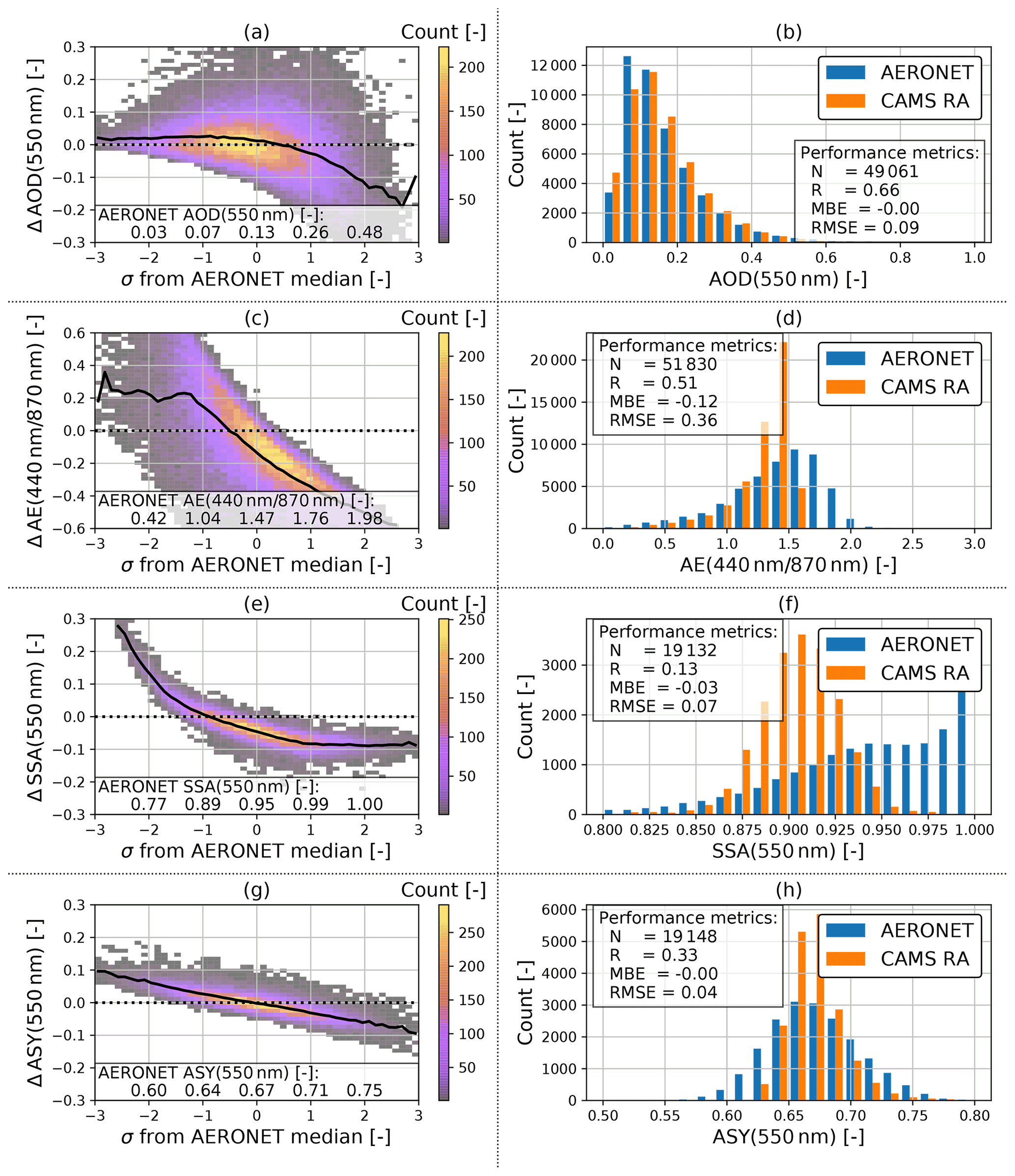
Figure 3Evaluation of the CAMS RA aerosol properties database versus AERONET aerosol products in Germany in the period from 2003 to 2019. Left panels show the deviation of a quantity (CAMS RA – AERONET) on the left y axis as a 2D histogram and the mean as a black line. The values on the left panels are plotted versus quantiles (number of standard deviations σ from median) of the AERONET distribution. The right panels show the dataset distribution of each quantity and calculated evaluation metrics.
Figure 3 shows the comparison and evaluation statistics for all considered aerosol parameters. The difference of the CAMS RA and the AERONET properties are shown on the left panels. In order to facilitate a better overview of in which part of the distributions an over- or underestimation occurs, the difference from the median value of the AERONET variable expressed in multiples of the SD is plotted on the x axis. In the panels on the side, the distributions of the aerosol optical properties from AERONET and CAMS RA are compared.
The CAMS RA AOD at 550 nm is on average in good agreement with the observations, as indicated by an MBE close to zero. Nevertheless, there is a slight overestimation of about 0.02 at AOD values below the median and an underestimation at higher AOD values. The instantaneous agreement shows a relatively wide dispersion, as indicated by a correlation of 0.66 and an RMSE of 0.09. This magnitude clearly exceeds the uncertainty estimate of the spectral AOD of AERONET of about ± 0.02 (Giles et al., 2019), which implies that the deviation is mainly due to the uncertainty of the aerosol properties in CAMS RA and possibly due to the collocation method used. Thus, a value of ± 0.09 is used here as an estimate of the CAMS RA AOD standard error.
For both datasets, the AE is calculated from the spectral AODs at 440 and 870 nm. According to AERONET, the AE varies around a mean value of about 1.5 over Germany, with about 95 % of the values lying between 0.4 and 2. In contrast, the AE values calculated from CAMS RA appear to be limited to values below 1.6 with a frequency peak at 1.5. This indicates that the limited set of aerosol classes used in CAMS RA cannot realistically represent aerosol mixtures with a strong spectral dependence of the AOD. The cases corresponding to AERONET AE values above 1.6 account for about 40 % of the total number of data points.
In consequence, spectral AOD values below and above 550 nm tend to be underestimated and overestimated, respectively. AE values below 1 are overestimated by CAMS RA, with a mean bias of about 0.2, which mainly affects aerosol with spectral flat properties (mineral dust).
The SSA values at 550 nm vary around a median value of 0.9 over Germany according to CAMS RA, with the shape of the distribution resembling that of a normal distribution with a full width at half maximum of about 0.05 and bounded between values of 0.8 and 0.98. On the other hand, the AERONET inversion product (Level 1.5) shows a much broader distribution of SSA values between 0.8 and 1, with a median value of 0.95. The SSA inferred by AERONET is clipped at a maximum value of 1 (no absorption), a value which is never reached by CAMS RA. In general, an overestimation of the amount of aerosol absorption in CAMS RA can be observed in comparison to AERONET (MBE = −0.03). This finding is important, because the SSA has a strong influence on the value of REari (see Sect. 4.1.2 and 4.1.3). Furthermore, the instantaneous comparison shows a wide scatter with an RMSE of 0.07. This indicates that the aerosol representation in CAMS RA has problems in reproducing the aerosol absorption based on the set of aerosol classes used in the underlying aerosol model. In comparison, the standard error of the AERONET SSA inversion is estimated to be about ± 0.03 (Dubovik and King, 2000; Sinyuk et al., 2020), with increasing uncertainty at lower AOD values (± 0.08 for AOD below 0.1 and ± 0.05 for AOD values between 0.1 and 0.2; Sinyuk et al., 2020). It should be noted that, for comparisons in this study, the AERONET SSA is calculated from the ratio of absorption and extinction AOD at 440 nm, which are transferred to 550 nm using the Ångström relation (Eq. 2). Therefore, the uncertainty for the AERONET SSA might be larger than the proposed values.
In agreement with CAMS RA and AERONET, the ASY at 550 nm is distributed around a median value of 0.67. However, the distribution of CAMS RA ASY values is more narrow, having a range from 0.62 to 0.76, while ASY values from AERONET span a range from 0.56 to 0.79. Besides this difference, the comparison shows an RMSE of 0.04, which, again, is well above the uncertainty estimate of ± 0.01 for the ASY retrieved by AERONET (Sinyuk et al., 2020). Therefore, the standard error of ASY from CAMS RA is estimated to be about ± 0.04.
A subset of the data for the year 2015 has been used to identify possible outliers or unique aerosol conditions during this year (see Fig. D1). The 2015 subset shows similar aerosol and comparison statistics to those for the complete period from 2003 to 2019. This indicates that the aerosol conditions over Germany during the year 2015 did not differ significantly from the long-term mean conditions. Thus, the year 2015 is considered to be representative and is used for the further analyses of this study.
The comparison results for AOD and AE from CAMS RA and AERONET reported here are consistent with several previous studies. Inness et al. (2019a) compared CAMS RA AOD at 550 nm and AE(440, 870 nm) against measurements from AERONET stations for the period from 2003 to 2016. Similar to our study, they found an insignificant underestimation of AOD (MBE = −0.003) compared to European AERONET stations. Compared to global AERONET stations, a correlation of 0.8 to 0.9 was reported for AOD. For AE, an overestimation of 5 %–20 % and a correlation of 0.6 to 0.7 was found. These results show a higher degree of agreement and a positive instead of the negative bias obtained in the present study. Our study is however limited to the region of Germany, which may explain a lower correlation, due to lower AOD values and a more narrow distribution of AE in comparison to global aerosol conditions. Furthermore, the global mean of AE values is about 1.2 (Inness et al., 2019a) versus the value of 1.5 over Germany, and a positive bias for smaller AE values is also observed for CAMS RA within the present study. Another long-term evaluation of CAMS RA AOD and AE for the period from 2003 to 2017 versus AERONET was performed by Gueymard and Yang (2020). For the European region, they found an MBE of 0.01 and an RMSE of 0.09 for AOD, which is consistent with the results of this study (0 and 0.09, respectively). While our study finds a slight underestimation of AOD, this result lies within their proposed uncertainty range. Furthermore, it is shown here that the bias between CAMS RA and AERONET AOD depends on the magnitude of AOD, which implies that the MBE strongly depends on the current aerosol conditions. Evaluating the AE over the European region, Gueymard and Yang (2020) found an MBE of −0.02 and an RMSE of 0.33, again similar to our results (−0.12 and 0.36, respectively). Other studies (e.g. Witthuhn et al., 2020; Zhang et al., 2020) assessing the AOD and AE of CAMS RA show that the AOD at 550 nm is well represented in CAMS RA. The level of agreement for AE, on the other hand, suffers from its restriction to values below 1.6 and, at the same time, from a positive bias for AE values below 1. When calculated from the Ångström relation, the spectral AOD at other wavelengths may be biased as a consequence of this behaviour.
The representation of the intrinsic aerosol optical properties SSA and ASY in the CAMS RA has not, to our knowledge, been evaluated in other studies. Our results show that the realistic representation of aerosol absorption as represented by the SSA is a weak point of CAMS RA in its current form. The SSA is generally underestimated compared to the AERONET inversion product, indicating a significant overestimation of aerosol absorption. This aspect is important because, when CAMS RA aerosol properties are used as input for radiative transfer calculations, it will lead to excessive atmospheric heating by aerosols, together with an underestimation of the DHI at the surface and the planetary albedo at the top of the atmosphere. This aspect is thus potentially of interest for studies of the impact of aerosols on the climate system using CAMS RA aerosol properties as basis and should therefore be further investigated and potentially corrected.
The overestimation of aerosol absorption will also have an impact on PV power potentials derived from CAMS RA. The PV power will be underestimated if CAMS RA aerosol properties are used as an input of radiative-transfer models with coupled PV power used for solar system planning. In addition to the positive bias in aerosol absorption, CAMS RA does not reproduce the full range of natural variability in either SSA or ASY, which can probably be attributed to the limitations of using a fixed set of aerosol types in the underlying aerosol representation. However, due to the wavelength-dependent spectral response of PV modules, uncertainties in wavelength-dependent aerosol properties will lead to uncertainties in PV power calculations. Nevertheless, in comparison to SSA, ASY is well represented in CAMS RA, as the MBE is close to zero and the RMSE has a value of 0.04. Therefore, the influence of the ASY uncertainty on simulations of solar irradiance and REari is expected to be minor.
4.1.2 Sensitivity of irradiance and REari
To analyse the sensitivity of T–CARS simulations to perturbations of the aerosol optical properties AOD, AE, SSA and ASY, the column amounts of O3 and H2O, and the surface albedo, radiative kernels are utilized using the approach of Thorsen et al. (2020) as basis (see Sect. 3.3.4).
The radiative kernels calculated for a 1 % increase in the corresponding parameter are shown in Fig. 4. They are displayed as vertically integrated annual-mean values over Germany for the year 2015 for both the GHI and DNI irradiance (panel a). The REari kernels at the surface and top of the atmosphere are shown in panel (b). An increase of 1 % in AOD(550 nm), for example, would lead to a change in annual REari by −84 mW m−2 at the surface and −42 mW m−2 at the TOA.
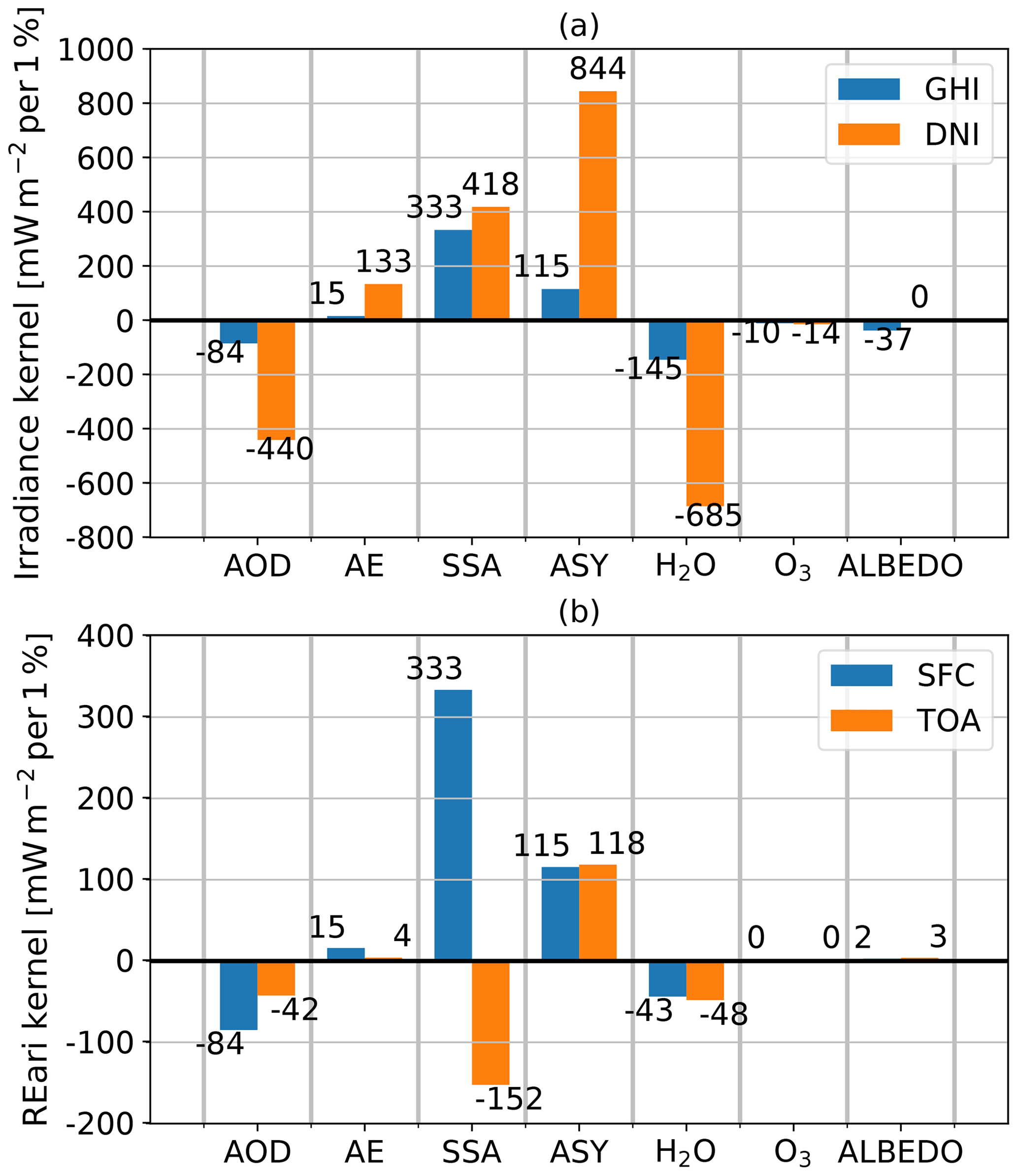
Figure 4Irradiance and REari kernel calculated for perturbations of 1 % of different variables in the ecRad radiation scheme. The calculations are conducted for the surface (blue) and top of the atmosphere (orange).
For the irradiance kernels, the DNI is always more sensitive to a change in a certain parameter, since the DNI is defined normal to the sun beam and thus has larger daily average values. An increase in AOD leads to decreasing values of GHI and DNI at the surface. The GHI is less sensitive to a change in AOD as, depending on the absorption properties of the present aerosols, a part of the scattered radiation is transferred from the direct beam into the DHI, leading to partial cancellation of the changes in GHI. In general, parameters increasing atmospheric absorption (AOD, water and ozone) decrease the surface irradiance. An increase in AE leads to a decrease in AOD at wavelengths longer than 550 nm and thus to an increase in surface irradiance, as this part of the spectrum makes up the largest contribution to broadband irradiance. Similar to AOD, the GHI is less affected by changes in AE. An increase in the amount of scattered radiation (increased SSA) will lead to an increase in GHI, as some fraction of this radiation will reach the surface. To solve the radiative transfer, the scattered fraction of radiation from the direct beam is reduced with the δ-Eddington scaling by a factor depending on ASY (Hogan and Bozzo, 2018). Therefore, the DNI is also sensitive to changes in SSA and ASY. An increase in SSA leads to more scattering and in turn increases the proportion of non-scattered radiation due to the scaling, which increases the DNI. This scaling factor is increased by an increase in ASY. Therefore, an increase in ASY will also affect the DNI. A change in surface albedo only affects the GHI, as a fraction of the irradiance reflected by the surface is back-scattered towards the surface, whose magnitude depends on the scattering properties of the atmosphere.
For the REari kernels, the sign of the response to perturbations is equal at the surface and top of the atmosphere, except for the SSA. The magnitude of the individual kernels is strongly dependent on the scattering properties of the aerosol mixture. For SSA, a changing sign at the surface and top of the atmosphere is found, as an increase in SSA reduces atmospheric absorption. Thus, the downward irradiance and net flux at the surface increase with SSA (shown in panel a), leading to a positive REari kernel. On the other hand, the upward irradiance at the TOA will also increase with increasing SSA, which reduces the value of the net flux at the TOA, leading to a negative sign of the REari kernel. For the REari kernels for aerosol perturbations at the surface, it has to be noted that they are equal to the GHI kernels, as a change in these properties only affects the irradiance simulated with aerosol radiative effects (see Eq. 1). The REari kernels for parameters which affect the irradiance with aerosol and in pristine conditions show generally lower values for pristine conditions, as the sensitivity is larger than in the presence of aerosols.
The different clear-sky radiative kernels show that the value of surface irradiance and REari is most sensitive to changes in SSA, followed by ASY and AOD, according to a 1 % change in each individual parameter. In addition, the surface irradiance also depends strongly on the amount of atmospheric water vapour. The difference between the surface and top-of-atmosphere REari kernels (surface − top of atmosphere) shows an increase in atmospheric heating by aerosols if it is negative and an atmospheric cooling if positive. Therefore, an increase in AOD leads to increased atmospheric heating, while increasing SSA leads to atmospheric cooling due to a reduction in aerosol absorption. Other parameters do not strongly affect atmospheric heating or cooling. The REari of the total atmosphere is most sensitive to variations in AOD and SSA, followed by ASY.
Since an increase of 1 % in all variables is unrealistic, the REari uncertainty is investigated by scaling these kernels by realistic uncertainty estimates of the observed parameters in Sect. 4.1.3.
4.1.3 Uncertainty of irradiance and REari
To estimate the systematic and random uncertainties of clear-sky irradiance and REari from T–CARS, the simulated radiative kernels are scaled with the values of MBE and RMSE, respectively, calculated for the optical properties of the aerosols from CAMS RA in Sect. 4.1.1. The results are shown in Figs. 5 and 6. Only the aerosol optical properties are shown, since the influence of the atmospheric parameters on REari uncertainty is negligible.
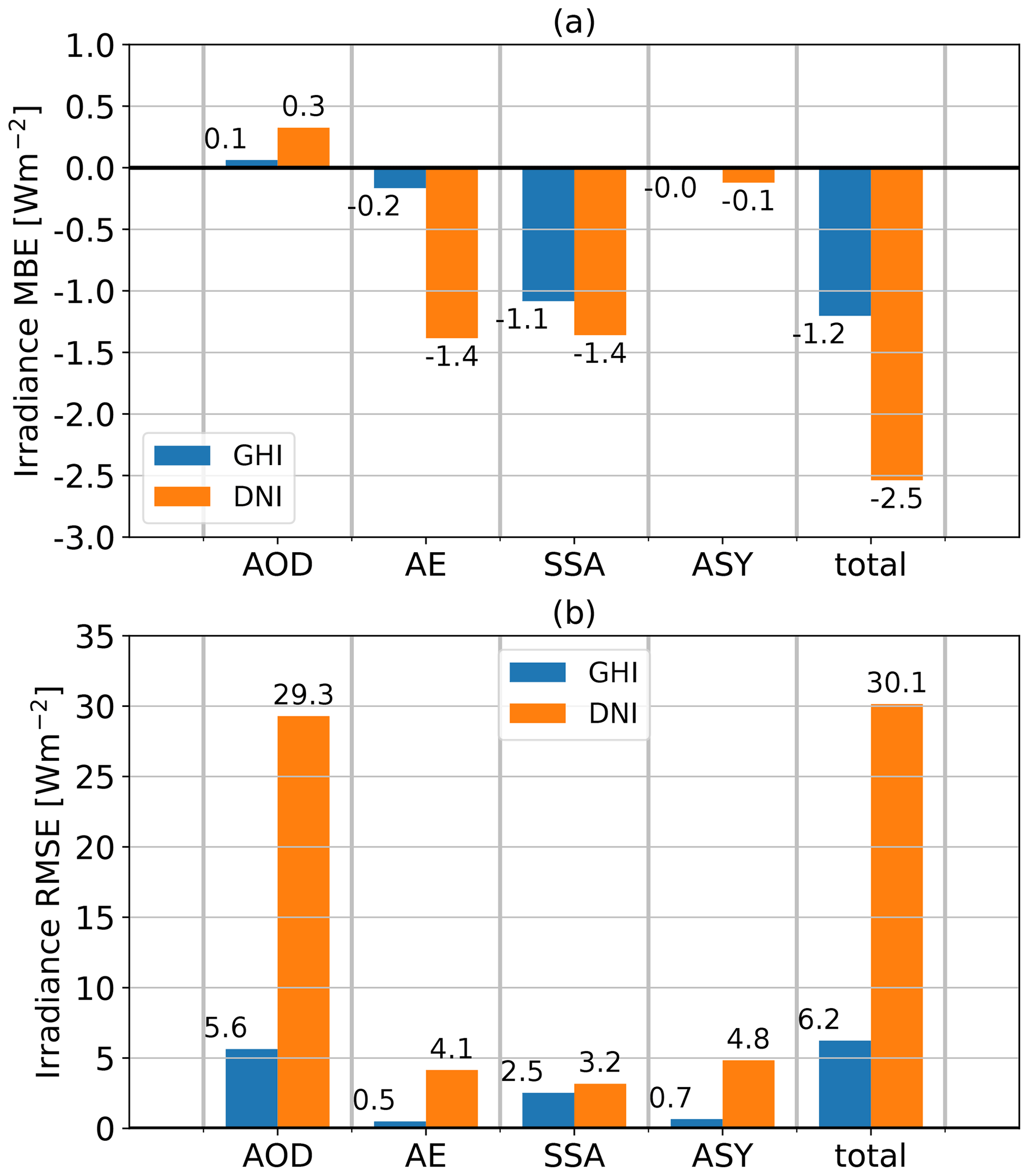
Figure 5Mean bias (a) and RMSE (b) estimates of simulated GHI (blue) and DNI (orange). The estimates are computed from irradiance kernels weighted by MBE and RMSE of the CAMS RA aerosol optical properties compared to the AERONET aerosol products.
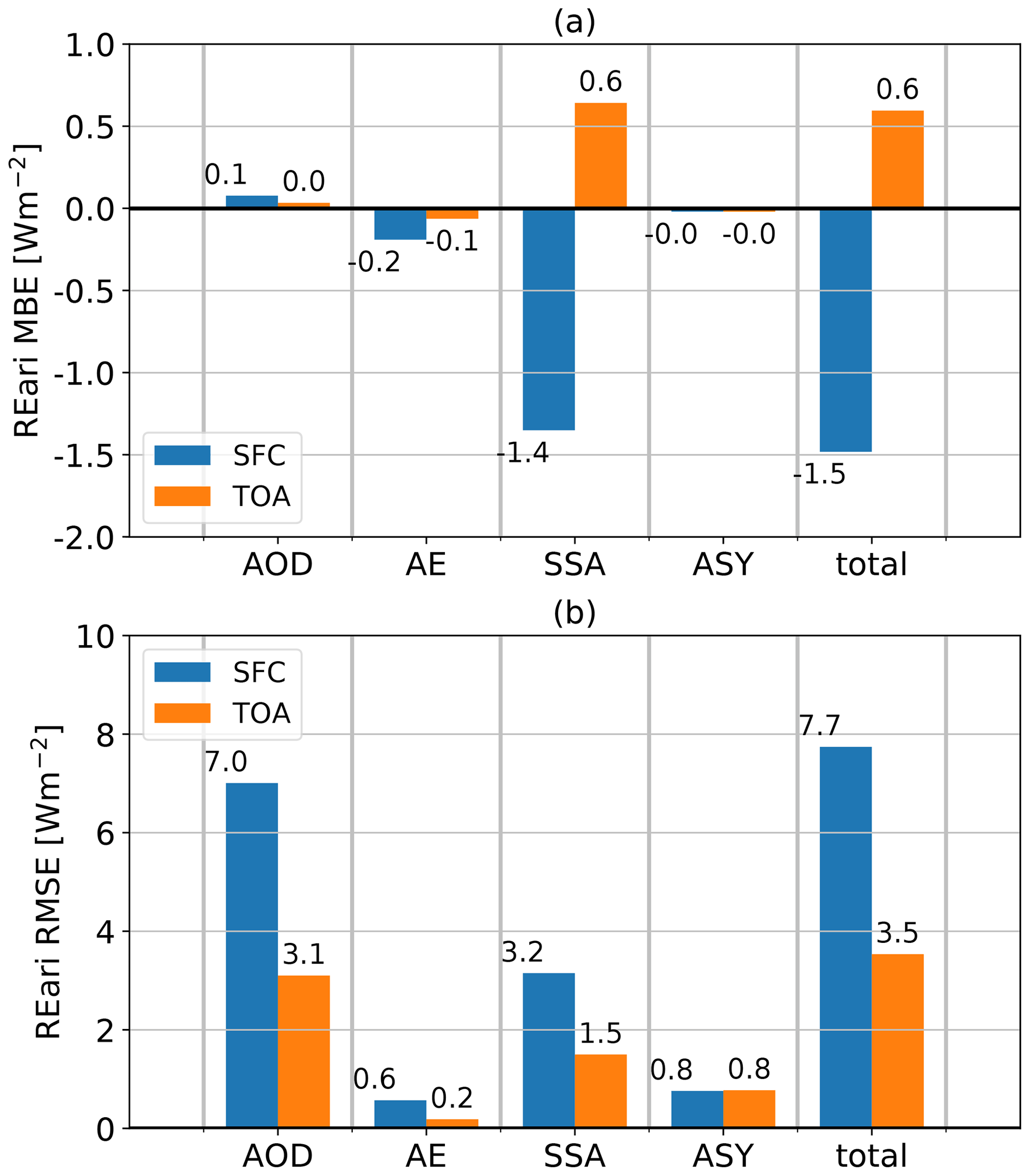
Figure 6Mean bias (a) and RMSE (b) estimates of simulated REari at the surface (blue) and top of the atmosphere (orange). The estimates are computed from REari kernels weighted by MBE and RMSE of the CAMS RA aerosol optical properties compared to the AERONET aerosol products.
For irradiance and REari, the major contribution to the MBE is the SSA uncertainty, and the major contribution to the RMSE is the AOD and SSA uncertainty of CAMS RA. As the ASY is represented well in CAMS RA, its contribution is almost negligible. The biases of the simulated variables are dominated by the overestimation of aerosol absorption in CAMS RA. In consequence, surface irradiance and REari are underestimated, and REari at the top of the atmosphere is overestimated. For DNI, AE is also a major contributor to deviations, as it determines the aerosol optical depth and thus the amount of scattering and absorption at longer wavelengths relevant for broadband solar irradiances.
Regionally, the REari MBE and RMSE do not show a large variance (see Fig. D2). The MBE ranges between −2 and −1 W m−2 at the surface, between 0 and 1 W m−2 at the TOA, and between 1.5 and 2.5 W m−2 for the total atmosphere. The RMSE values are about ± 7 W m−2 at the surface and ± 3 W m−2 at the TOA. The RMSE is largest in the southern part of Germany. This is the result of the combination of stronger incident radiation and lower AOD values, as AOD is the main contributor to REari RMSE.
For comparison, the REari kernels are also scaled with the AERONET uncertainties documented in Giles et al. (2019) and Sinyuk et al. (2020). The result is shown in Fig. D3. According to this approach, the REari is most sensitive to AOD followed by SSA and AE, which agrees well with the results obtained based on the uncertainty of the CAMS RA input data shown in Fig. 6.
4.2 Irradiance and REari simulations with T–CARS and CSM
In this section, the results of irradiance and REari retrieval using CSMs and simulations from T–CARS are intercompared and evaluated with reference observations. First, the consistency of the pristine irradiances calculated with the different CSMs is tested (Sect. 4.2.1) to investigate the influence of different assumptions for the atmosphere and aerosol on the accuracy of the predicted clear-sky irradiance and REari. Next, the clear-sky irradiances from the CSMs and T–CARS are compared to reference observations from the DWD station network (Sect. 4.2.2). Finally, the resulting REari values from the CSMs and T–CARS are intercompared in order to establish their accuracy and consistency (Sect. 4.2.3).
4.2.1 Intercomparison of pristine irradiance simulations
The pristine irradiance can be calculated with the CSMs selected for this study by setting their AOD input to zero. The assumptions made for atmospheric transmittance for atmospheric gases and other factors used by the CSMs then determines their accuracy. Since the CSMs were not originally designed to provide accurate estimates for a hypothetical pristine situation, non-physical results and large deviations are possible. The irradiance under pristine conditions is, however, required as reference for the calculation of the REari (see Eq. 1). Thus, the accuracy of the irradiances predicted by the CSM under pristine conditions is compared here to the T–CARS simulations to assess their consistency. The results of the comparison for GHIpri and DNIpri are shown in Table 3.
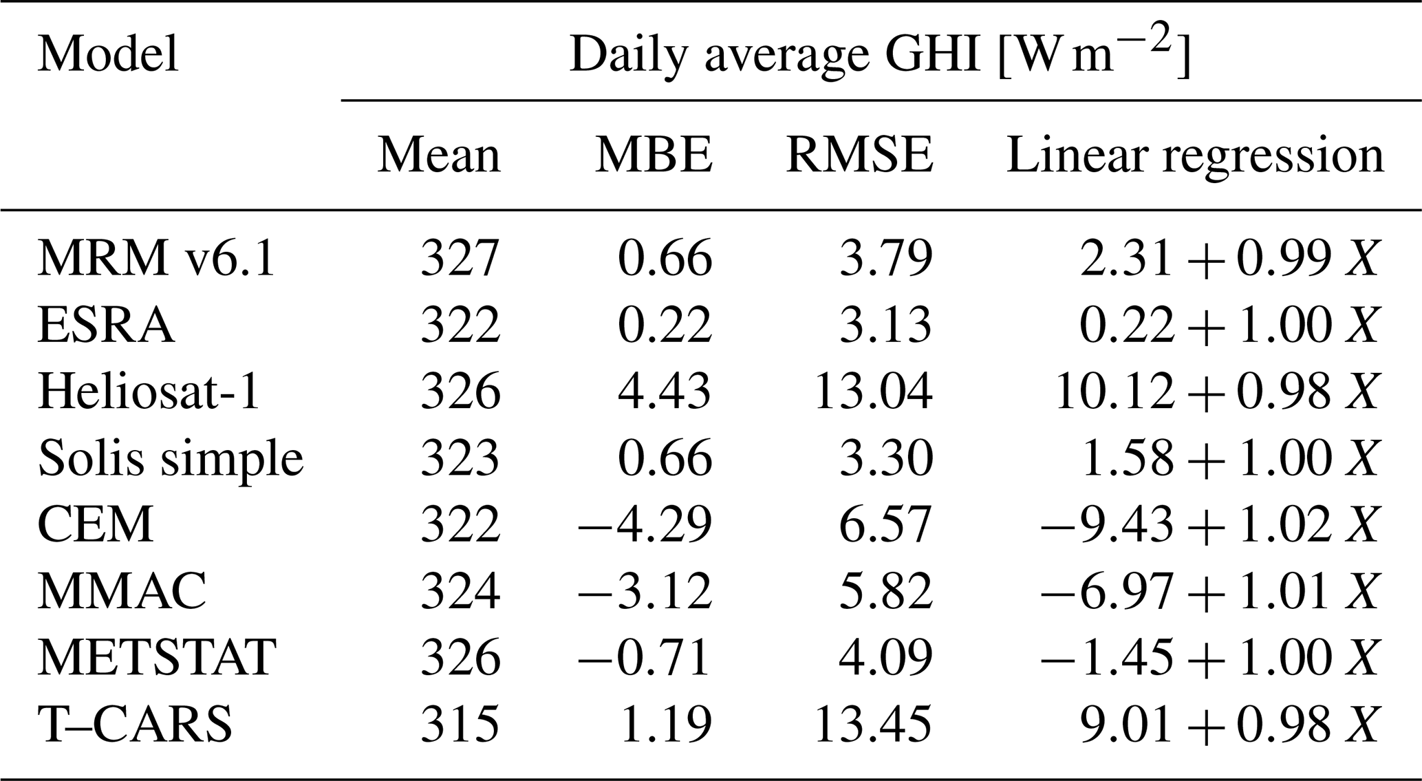
Table 3Comparison of the annual mean of daily average values of GHI and DNI in pristine (pri) conditions (AOD = 0) simulated with each CSM compared to T–CARS and daily mean GHI and DNI at the surface with aerosols comparing CSM and T–CARS to observations. Note that the number of days available for comparison varies between models. In addition to MBE and RMSE, the linear regression function is shown with reference irradiance simulated with T–CARS denoted as X. The correlation of CSM and T–CARS values are always larger than 0.99

In comparison to the T–CARS simulations, the best level of agreement for GHIpri is found for the models MMAC and Solis simple, with an MBE below 1 W m−2 and an RMSE below 3 W m−2. For the DNIpri, the best agreement is again shown by the Solis simple model. The Solis simple model is based on a large set of radiative transfer simulations, which include simulations with an AOD value of zero (see Sect. A4). Therefore, the good agreement between T–CARS and the Solis simple model is not surprising. Apart from Solis simple, the representation of a hypothetical pristine irradiance in other CSMs is less accurate, as they are mostly optimized to represent the measured irradiance under natural conditions, which of course always contain some aerosol content. The models Heliosat-1 and ESRA have similar formulations for the DNI, which is also reflected in the comparison results of Table 3. The GHI in these models is calculated from the DNI and DHI components. The DHI in Heliosat-1 and ESRA depends on the Linke turbidity at an air mass of 2 (see Sect. A2, Louche et al., 1986), but the models use different empirical relations from Dumortier (1995) and Rigollier et al. (2000), respectively. According to the results of Table 3, the Dumortier (1995) estimate of the DHI better reproduces the conditions over Germany. Nevertheless, all CSMs except the CEM model agree well with the T–CARS model used as reference here, having biases smaller than ± 10 W m−2. The CEM model shows a large overestimation of the pristine irradiance, which is likely due to the neglecting of ozone absorption.
The biases found here for the GHIpri will propagate directly into the REari retrieval of the CSMs. An overestimation of the pristine irradiance will lead to a stronger radiative effect. Therefore, it is expected that the magnitude of REari is overestimated by MRM v6.1, ESRA and most strongly by the CEM model, while an underestimation of the magnitude of REari inferred from the METSTAT model is expected.
4.2.2 Comparison of clear-sky irradiance simulations to DWD observations
In this section, the simulated irradiances from the CSMs and the T–CARS setup considering aerosol effects are evaluated by a comparison to reference observations in clear-sky conditions from the DWD station network.
In Table 4, the daily average values of GHI are compared. For the CSMs, the results are an indicator for the quality of the clear-sky fitting method (see Sect. 3.2), as results are fitted to the observations on a daily basis. The deviation of the CSMs from observations given in the table can be attributed to the underlying definition of the atmosphere and aerosols in the CSMs, which might not realistically reproduce the diurnal cycle of irradiance. Despite the use of similar definitions by the ESRA and Heliosat-1 models, the Heliosat-1 model shows the largest random deviations in this comparison, as solar refraction is not corrected in the air mass calculation. The highest level of accuracy is achieved by the models Solis simple, ESRA, METSTAT and MRM v6.1, which show lower values of MBE than the T–CARS results. Unlike the CSM results, the simulations of the T–CARS setup are not adjusted to the observations. Therefore, the deviations shown in Table 4 can be attributed to the uncertainty of the CAMS RA inputs, in combination with the collocation method and altitude correction for the station location.
Table 4Comparison of the annual mean of daily average values of GHI at the surface simulated with each CSM and T–CARS compared to DWD observations. Note that the number of days available for comparison varies between models. In addition to MBE, RMSE and correlation (R), the linear regression function is shown with reference irradiance measured by DWD denoted as X. The correlation of retrieval and observation is always larger than 0.99.
In the following, a detailed comparison of the T–CARS simulations and the DWD observations is presented. Here, the added value of the CAMS RA aerosol information for the simulation of solar irradiance is tested using the following equation:
where σ denotes the SD and F either one of GHI, DHI or DNI. The subscripts pri and aer indicate the simulated irradiances in pristine conditions and in the presence of aerosols, respectively. Observed irradiance is denoted by the subscript obs. For this metric, the SDs of two simulations for the same reference dataset are compared. Therefore, the SDs can be compared directly, and a positive difference, Δσ (Eq. 9), indicates a higher level of agreement of the simulation considering aerosols. A positive Δσ is expected, as long as the aerosol properties provided by CAMS RA as input to ecRad improve the simulation of the surface irradiance components. Applied to the DNI, this test shows the accuracy of the column-integrated aerosol extinction obtained from CAMS RA, given by AOD and AE. For GHI and DHI, the simulated irradiances also depend on the representation of aerosol scattering and absorption properties characterized by SSA and ASY.
The results of the comparison are presented in Tables 5, 6 and 7 for DNI, GHI and DHI, respectively. The RMSE and MBE of simulated and observed irradiance values are listed together with the mean value found for the entire observation period. Two correlation values are given: first, the correlation comparing the observed and simulated irradiance (R(Faer,Fobs)), and second the correlation of the simulated and observed aerosol radiative effect (). For the latter, a high value of correlation indicates a good representation of the aerosol radiative effect based on CAMS RA. The last metric presented in the tables is Δσ of Eq. (9). Positive values of Δσ indicate a positive impact of the aerosol inputs obtained from CAMS RA for the T–CARS simulation on the agreement between simulated and observed irradiance, due to aerosol information obtained from CAMS RA in ecRad. All metrics are also given for different station selections (e.g. coastal or mountain stations; see Fig. 2 and Table 1). Also, a comparison for different seasons is included.
Table 5T–CARS direct normal irradiance with aerosols (DNIaer) and in pristine conditions (DNIpri) compared to DWD observations (DNIobs). Annual average values are represented by an overline (e.g. ). The RMSE and MBE are shown for the comparison of DNIaer and DNIobs. Correlations are shown for R(DNIobs,DNIaer) and . The level of agreement is evaluated by the difference of the SD of simulations in pristine conditions and with aerosols using Eq. (9) (Δσall).

The results presented in Table 5 show a relatively good level of agreement between simulated and observed DNI, with a reduction of the RMSE by about 20 W m−2 (Δσ) for all stations. The simulation of the DNI is highly correlated with the observations, showing a correlation larger than 0.95 for all cases and selections. The best agreement is found for the spring and summer seasons, the coastal and northern stations, and for the more temperate maritime climate (Cfb). These results can be explained for several reasons. First, the stronger solar radiation and the more absorbing aerosol in spring and summer lead to a mitigation of the systematic errors in the simulations (e.g. overestimation of absorption by CAMS RA) and measurements. In addition, larger AOD values are observed in spring and summer and at more northerly stations, which reduces the deviations due to random errors. Furthermore, the input data of CAMS RA are collocated and altitude-corrected for this comparison, and the uncertainties of this method are larger over complex terrain and mountains towards the south. However, the differences in the various selection criteria are very small, so these are only hypotheses. In most cases, the DNI simulated with T–CARS is overestimated, especially in winter. The values of RMSE indicate an acceptable uncertainty of about 5 % to 10 % versus the reference observation, given that the uncertainty of DNI of the DWD observations is estimated to be about 5 %. Therefore, about half of the uncertainty may be attributed to the uncertainty of the irradiance observations. This is consistent with the results on the sensitivity analysis of the irradiance simulations (Sect. 4.1.3), which reported about 50 % smaller RMSE values. The RARE values show an acceptable correlation above 0.7 in most cases, except for the winter and fall seasons. This could be due to the lower absorption properties of aerosol in winter and fall and generally lower AOD values in these seasons. Reduced absorption by aerosols leads to increased deviations due to overestimation of absorption in CAMS RA. Lower AOD values also mean a weaker radiation effect, making the simulation more prone to random errors. The good agreement for DNI is expected, since the DNI is strongly influenced by the AOD, and the CAMS RA AOD agrees well with AERONET observations (see Sect. 4.1.1). The MBE suggests an overestimation of DNI by the T–CARS simulations, although a slight underestimation of about −2.5 W m−2 is expected from the sensitivity study. As the DNI from the DWD observations is inferred by use of a shadow ring, this bias may be caused by the shadow ring correction applied to the DWD observations.
Table 6Same as Table 5 but for global horizontal irradiance (GHI). In addition, the diffuse-to-direct-irradiance ratio is calculated for observations (DDRobs) and simulated irradiance (DDRaer).
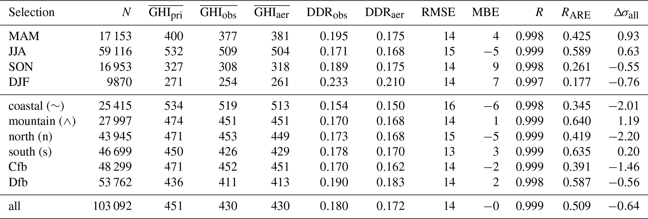
For GHI, a similar level of agreement as for DNI could be expected, as the GHI is usually dominated by the direct irradiance component in a cloud-free atmosphere. Table 6 shows, however, that this is only partly true. In general, the simulated GHI agrees well with the observation, as the correlation is never lower than 0.997, and the RMSE is always below 5 %. Also, the MBE shows smaller values than found for the DNI. However, regardless of location and season, all values of Δσ are distributed around zero, which indicates that there is little skill for the simulations of the instantaneous values of GHI. A plausible explanation is that the aerosol over Germany has only weak absorption, which will cause a redistribution of solar radiation from the DNI into the DHI based on the scattering properties of the aerosol. Hence, the aerosol effects on DNI and DHI partially cancel for the GHI, and thus differences are smaller between situations with and without aerosols. Therefore, no clear added value of the CAMS RA aerosol information is found for the T–CARS simulations. This is also reflected by the low values of correlation of RARE at northern and coastal stations, as well as in fall and winter. Additionally, Table 6 shows a comparison of observed and simulated diffuse-to-direct-irradiance ratio (, with μ0 being the cosine of the solar zenith angle) to investigate the distribution between the solar irradiance components. A lower value of the DDR is expected for stronger atmospheric absorption. The results show that the irradiances simulated by T–CARS always result in a negative bias of the DDR, regardless of the specific selection. This indicates an overestimation of atmospheric absorption in the model as long as the total extinction is well represented and is consistent with the overestimate of aerosol absorption reported before.
Table 7Same as Table 5 but for diffuse horizontal irradiance (DHI).
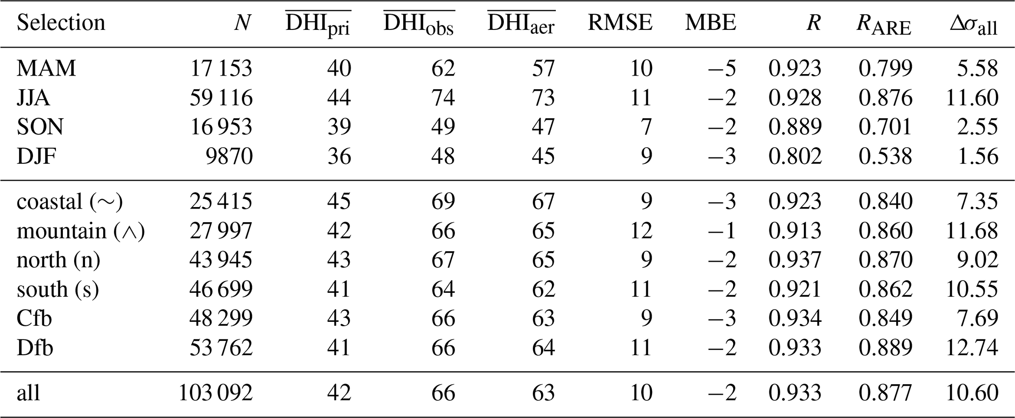
The hypothesis of an aerosol absorption that is too strong in CAMS RA is also supported by the DHI comparison shown in Table 7. Again, a good level of agreement similar to the metrics of the DNI evaluation is found. While the RMSE has a magnitude of 18 % relative to the observations, observations and simulations are strongly correlated, as indicated by R values of >0.88, except for winter (R=0.8). The lowest values of correlation RARE for DHI are found for the fall and winter seasons, with values of 0.7 and 0.5, respectively.
A larger bias and lower correlations during the winter are expected, since the lower sun elevation and amount of incident solar radiation increase the atmospheric path length and the measurement uncertainty. In general, the DNI simulated by T–CARS is overestimated by about 10 %, while GHI and DHI are both underestimated. Furthermore, the diffuse-to-direct-irradiance ratios presented in Table 6 show a negative bias by the model. This suggests an overestimation of aerosol absorption by CAMS RA and T–CARS, since the total aerosol extinction is represented well in CAMS RA (see Sect. 4.1.1).
A recent study by Marchand et al. (2020) evaluates the CAMS Radiation Service products and the HelioClim-3 database versus reference observations of all-sky and clear-sky irradiance at the DWD stations for the period from 2010 to 2018. The same DWD observations are utilized as reference in our study. The CAMS Radiation Service dataset provides broadband surface irradiance for clear-sky conditions based on the clear-sky model McClear. The input of atmospheric constituents and aerosol properties is also based on the CAMS RA as in this study. The comparison results under clear-sky conditions show an underestimation of about −101 to −55 W m−2 and a correlation above 0.85. These uncertainties are mainly attributed to the clear-sky identification of the Heliosat algorithm. This demonstrates the benefit of the clear-sky detection based on the Bright–Sun algorithm and ground-based observations used in this study, which significantly exceeds the performance of the satellite-based cloud detection.
4.2.3 Intercomparison of REari estimates
In this section, the daily average estimates of REari based on CSMs and T–CARS are intercompared. The simulation from the T–CARS setup is used as reference. To avoid inconsistencies due to the surface albedo data used, the T–CARS REari is adjusted to match the surface albedo (LSA SAF) used for the CSM simulations (see Sect. 3.3.2). Note that numerous days had to be interpolated in order to fill the gaps in the CSM simulations caused by cloudy days which do not meet the CSF criteria (see Tables 1 and D2).
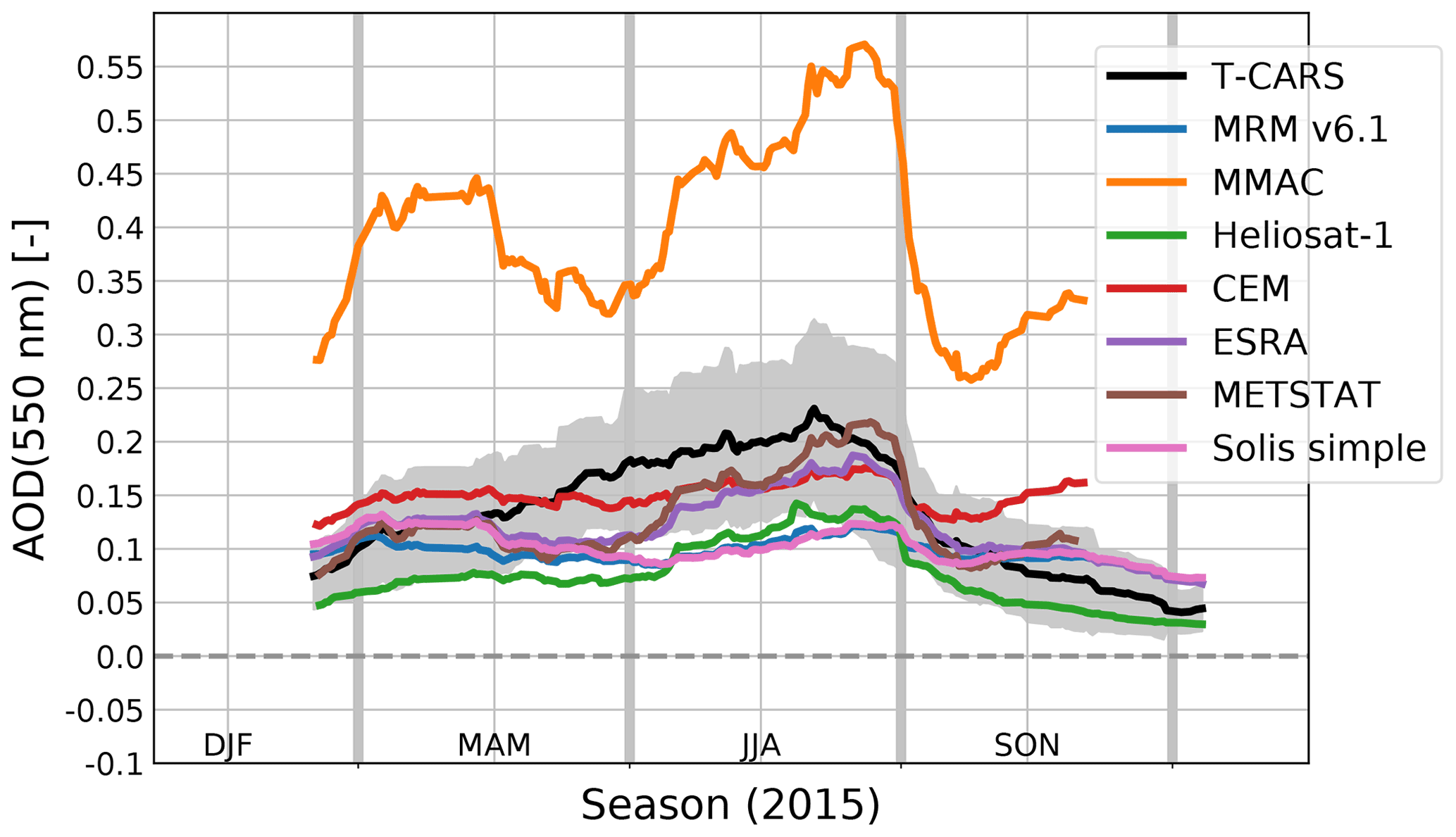
Figure 7Annual overview of average scaled AOD at 550 nm over all DWD measurement stations from CSF with different CSM compared to T–CARS. AOD values are shown as a 30 d rolling mean. For T–CARS the 30 d standard deviation is shown as a grey area.
Table 8Comparison of the annual mean of daily average AOD values, scaled to 550 nm. The values are averaged over all DWD stations and derived from CSF with different CSM. The reference AOD is calculated with T–CARS.
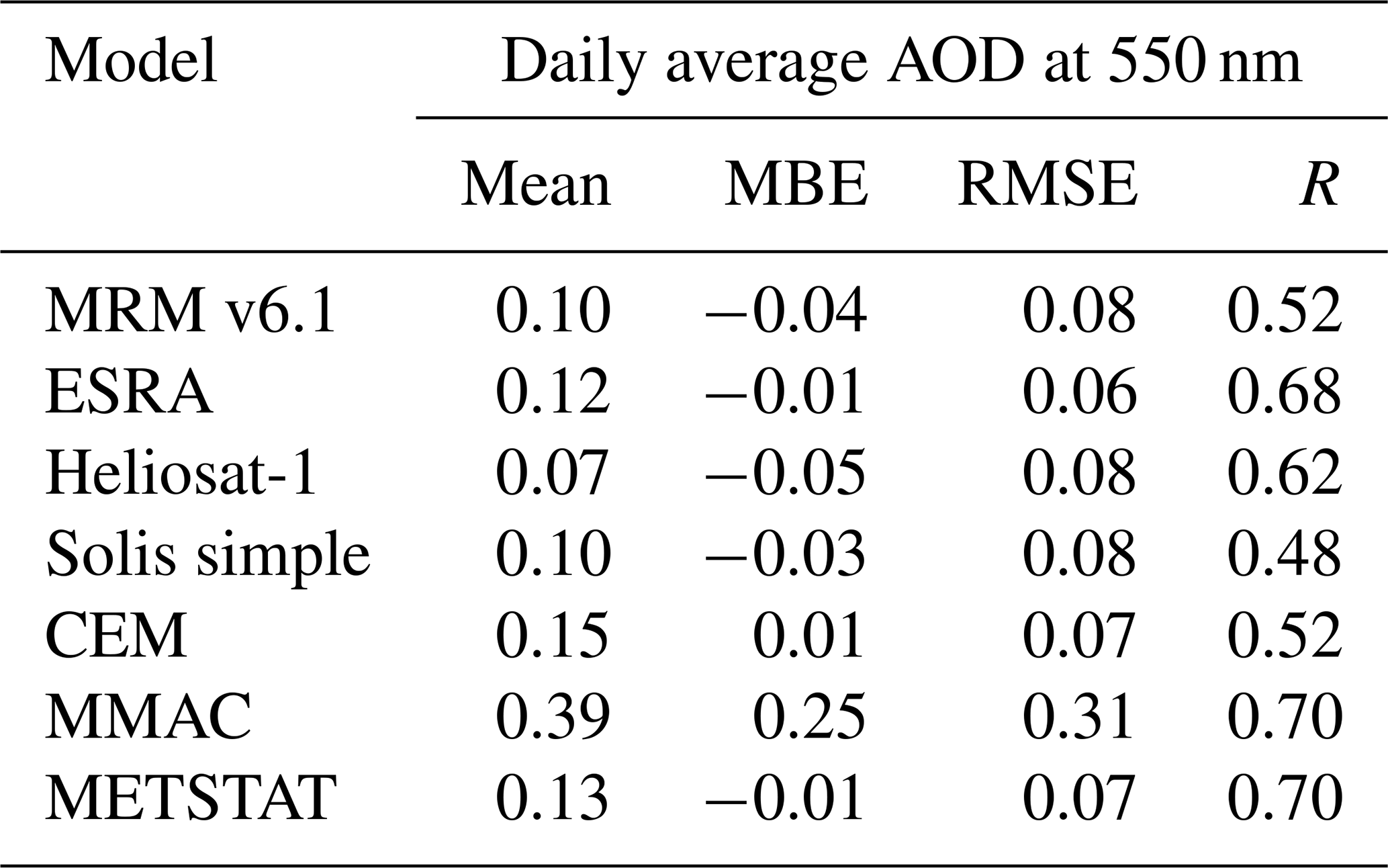
As the magnitude of the REari is mostly determined by the AOD, the AOD estimated with the CSMs is compared as a first step. The CSMs are based on the AOD at different spectral wavelengths: while the AOD at 550 nm is considered in the models MRM v6.1, ESRA and Heliosat-1, the AOD at 700 nm is considered in the simplified Solis model, and a broadband AOD is used in the models CEM, MMAC and METSTAT. These daily average AOD values are converted to a wavelength of 550 nm to increase the comparability of the CSM results. For the AOD at 700 nm, this is done using the AE(550, 700 nm) calculated with T–CARS. The broadband AOD is scaled to 550 nm using the ratio of the T–CARS broadband AOD and the AOD at 550 nm. These scaled values of AOD are compared to the T–CARS AOD in Fig. 7 and Table 8. Figure 7 shows the annual time series of AOD as the average over all DWD stations, comparing the AOD values used in T–CARS and retrieved by the CSMs. All values shown are smoothed by a 30 d rolling mean. This figure shows that in general the AOD can be reproduced by a CSM fit, especially for the winter and fall seasons with lower AOD values. During summer, having the largest AOD values, almost all CSMs underestimate the AOD. An exception is the AOD retrieved from the MMAC model, which is strongly overestimated throughout the whole year. These results are also reflected by Table 8, which shows absolute values of MBE below 0.05 for all models except MMAC, which has an MBE of 0.25. The best accuracy is shown by the ESRA, METSTAT and CEM models, with absolute MBEs of 0.01, RMSE values below 0.07 and correlations larger than 0.68. The strong overestimation by MMAC is likely the result of the assumptions on aerosol optical properties with a fixed value of 0.98 for the SSA, which nearly neglects absorption by aerosols. Since the scattering contribution of the aerosol extinction of radiation increases the diffuse irradiance, and thus also the global irradiance, a much higher AOD is needed to fit the MMAC global irradiance to the measurements. Due to the assumption of constant aerosol optical properties, the AOD values retrieved with the CSMs are not able to reproduce the annual variability shown by the T–CARS setup based on the CAMS RA data. It should be noted that this also applies to the MRM v6.1 model, which is designed to use four different aerosol types, which are selected based on the input AOD. The results indicate that this approach does not seem to improve the accuracy for retrieving the AOD as is done here.
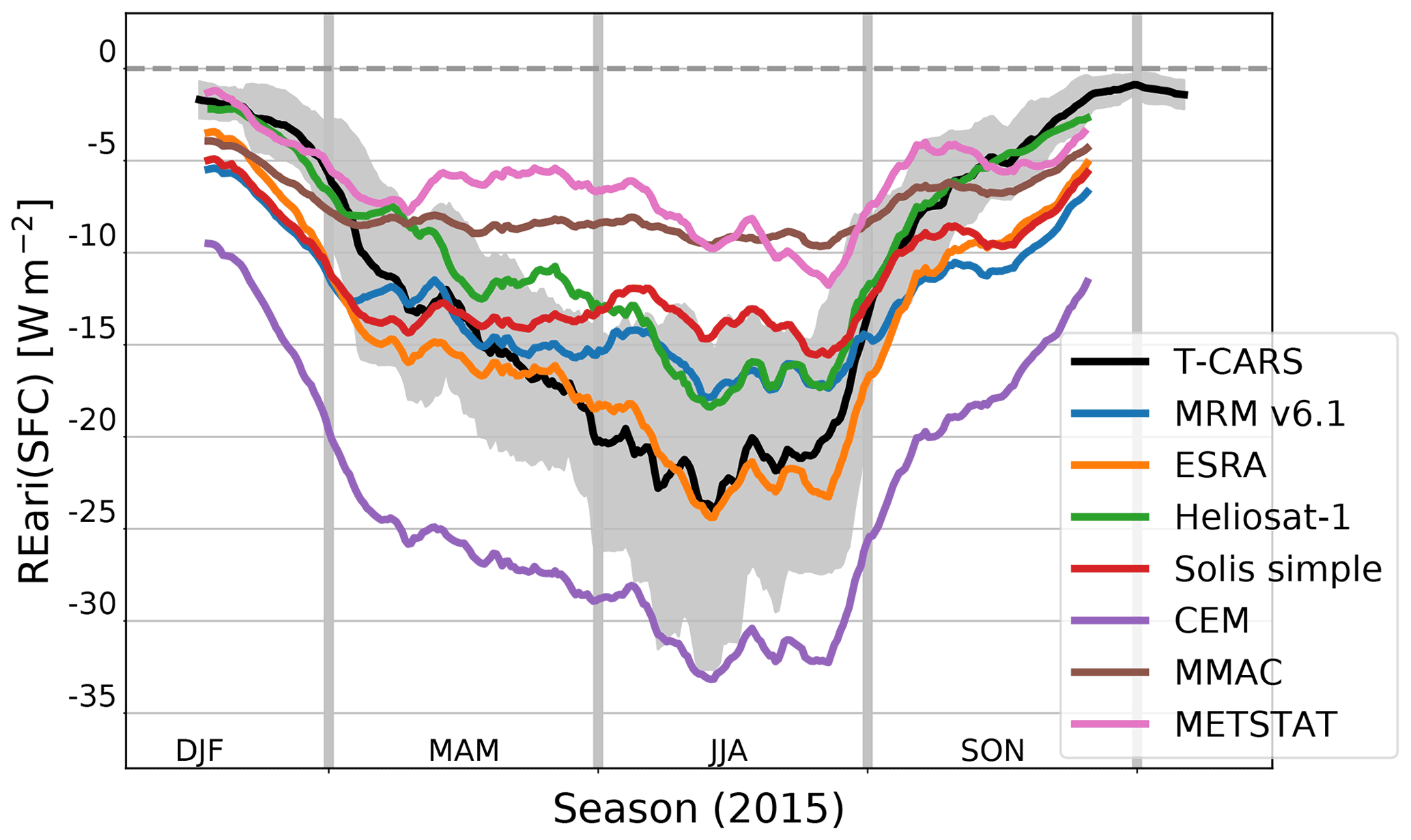
Figure 8The 30 d rolling mean of REari in the year 2015 utilizing different approaches. The shown REari values are computed as the mean over all DWD stations, while cloudy days are linearly interpolated over the year. The REari from T–CARS is simulated with collocated input to all DWD stations. In addition, for T–CARS, the 30 d rolling standard deviation (grey area) is shown.
Figure 8 shows the annual cycle of REari simulated by T–CARS (black line) in comparison to the values retrieved using the different CSMs (coloured lines). From day to day, the REari varies by up to ± 8 W m−2 around the rolling mean, as shown by the standard deviation (grey area) of the T–CARS REari. Figure 8 shows a pronounced annual cycle and large deviations between the different CSM-based estimates. Using the CEM model, the REari magnitude is strongly overestimated, which is caused by the overestimation of the pristine irradiance. However, the AOD inferred from the CEM model shows a reasonable accuracy. In the CEM model aerosol scattering is not considered; therefore, all aerosol extinction is attributed to absorption which drastically increases the attenuation of GHI with increased AOD values (see Table 2). On the other hand, the magnitude of the REari is strongly underestimated in summer, if the MMAC or METSTAT models are used. Oppositely to the CEM model, the MMAC-retrieved AOD is strongly overestimated in comparison to the CAMS RA-based AOD. On the other extreme, the SSA is fixed at 0.98, thus almost neglecting aerosol absorption and therefore strongly reducing the attenuating effect of aerosols for the global irradiance. The behaviour of the CEM and MMAC shows once again the importance of a realistic representation of the underlying aerosol optical properties in general and the influence of the SSA on REari in particular.
Table 9Annual mean of daily average values of the surface REari. The REari is simulated and averaged over all DWD measurement stations using CSM. The CSMs are sorted by performance of REari versus the T–CARS method indicated by the MBE, RMSE and correlation. In addition, the performance rankings of clear-sky irradiance estimates of the individual CSM are shown as proposed by Sun et al. (2019).
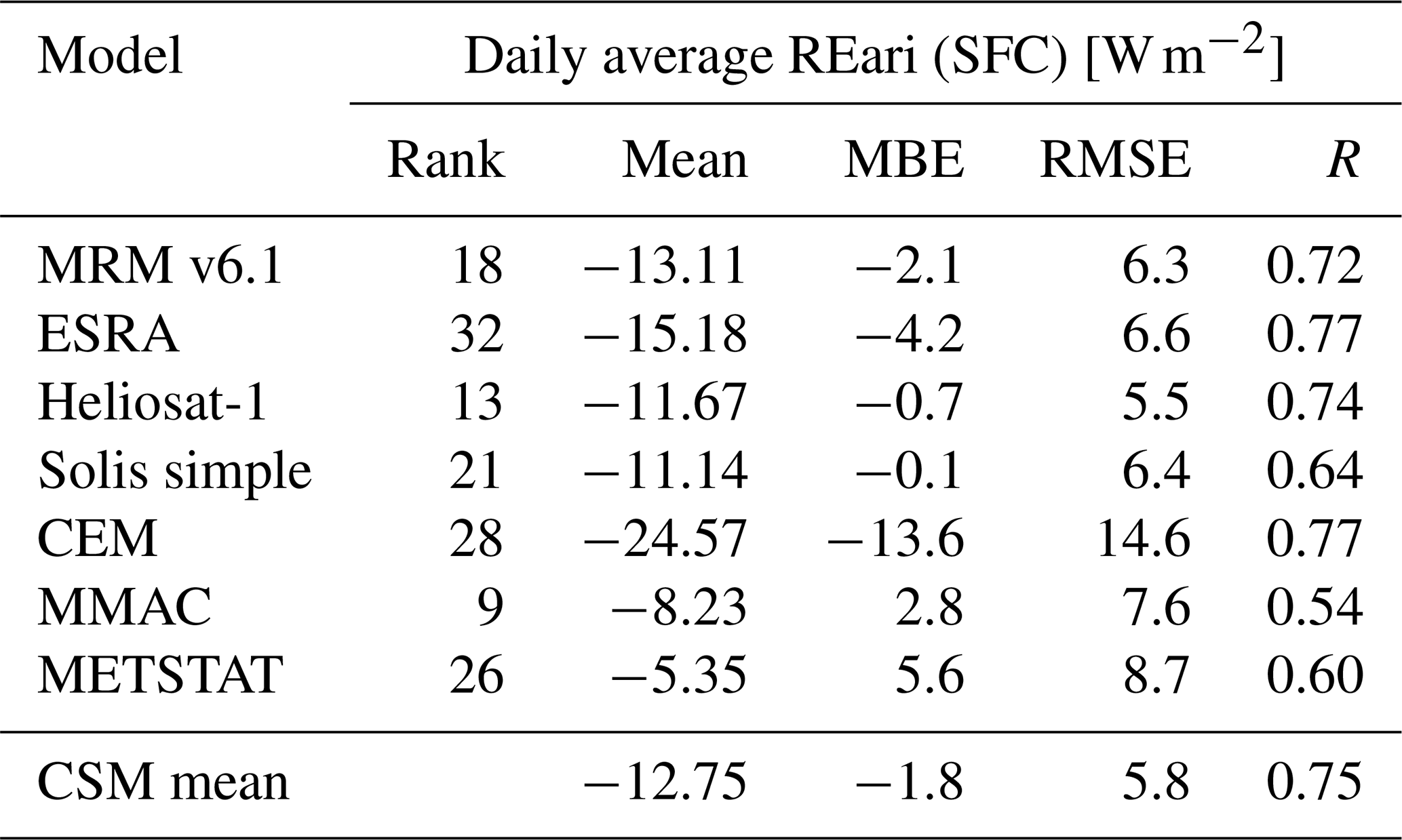
Most of the CSMs considered here are not able to reproduce the annual cycle of REari as simulated by T–CARS, due to the assumption of a fixed aerosol type by these models. Seasonal and annual-mean values of REari from the model- and observation-based approaches are presented in Table 9, along with comparison metrics versus the T–CARS simulations. The CSMs are sorted by performance, considering their individual MBE and RMSE values. The average annual value of REari from all observational approaches is −12.8 ± 5.5 W m−2 (± 2 W m−2 without CEM, METSTAT and MMAC), compared to −11 W m−2 simulated by the T–CARS. Therefore, this set of CSM seems to be able to reproduce the annual-mean results from T–CARS, despite the lack of an accurate annual cycle. For the individual CSMs, the highest level of agreement in the annual mean of REari is found for the MRM v6.1 model, with a deviation of −2 W m−2 and a correlation of 0.72. The ESRA model shows a larger MBE of −4 W m−2 but achieves the best correlation of 0.77. The ESRA model shows an overestimation of the absolute value of REari during the fall and winter seasons but is able to largely reproduce the annual cycle of REari as simulated by T–CARS.
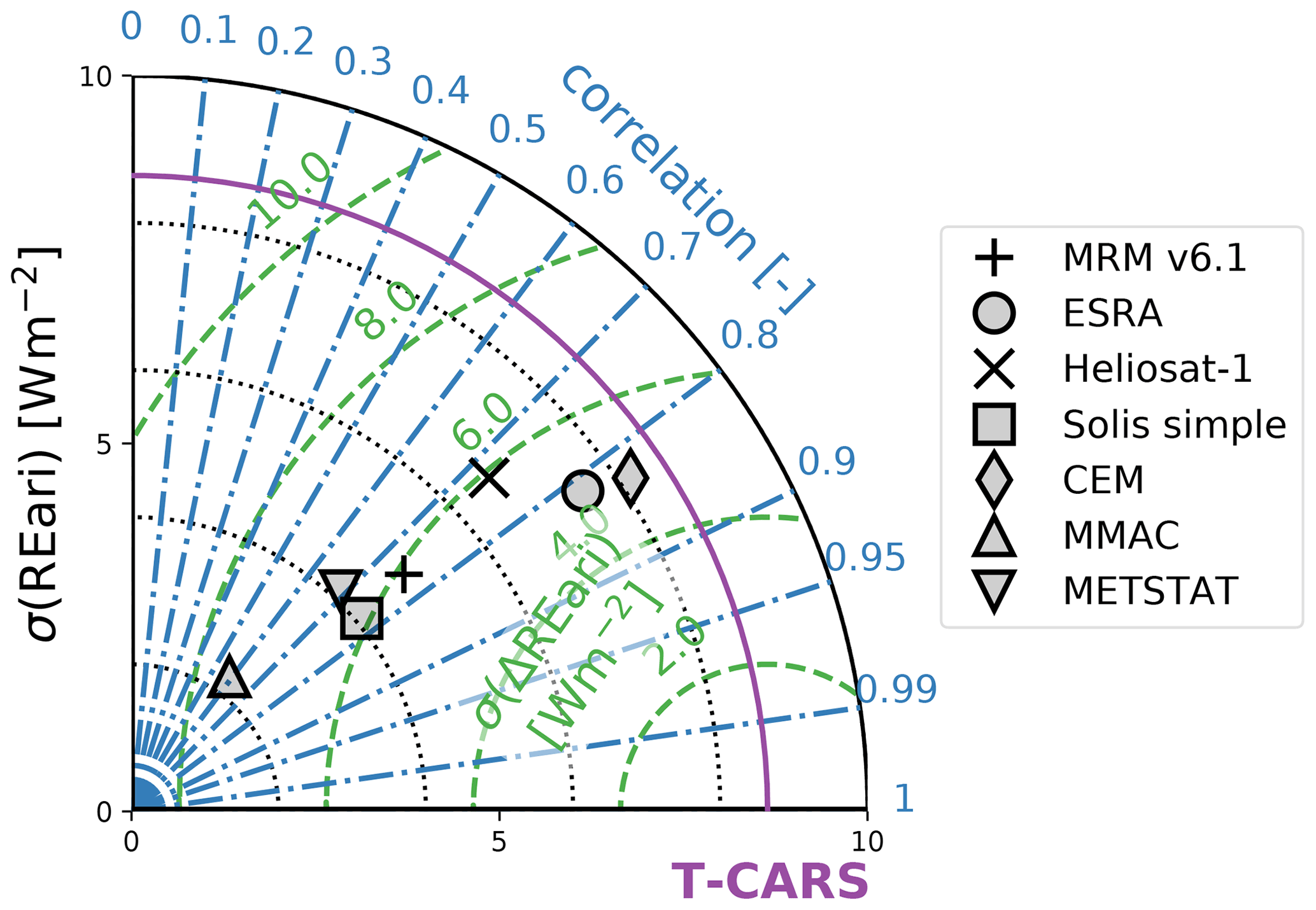
Figure 9The REari simulated with different CSMs as the average over all DWD observation stations is compared to the collocated T–CARS simulation. The annual variability is indicated by the SD (σ) of the individual dataset. The performance of the individual CSM is displayed by the SD of REari difference and correlation versus T–CARS.
Figure 9 presents the level of agreement between the individual CSMs and the T–CARS simulations in a Taylor diagram. The annual variability is expressed by the SD of the individual datasets and is shown as the radius in the diagram. For T–CARS, the annual variability value is about 8 W m−2. Further, the diagram shows the correlation (blue dashed lines) and the SD between the CSM and T–CARS values. Thus, the diagram expresses how well the annual cycle of REari is captured by the observational approach using the different CSMs. As the Taylor diagram does not account for biases of the compared values, the CEM model shows the best performance for reproducing the annual variability and correlation versus T–CARS, followed by the ESRA model.
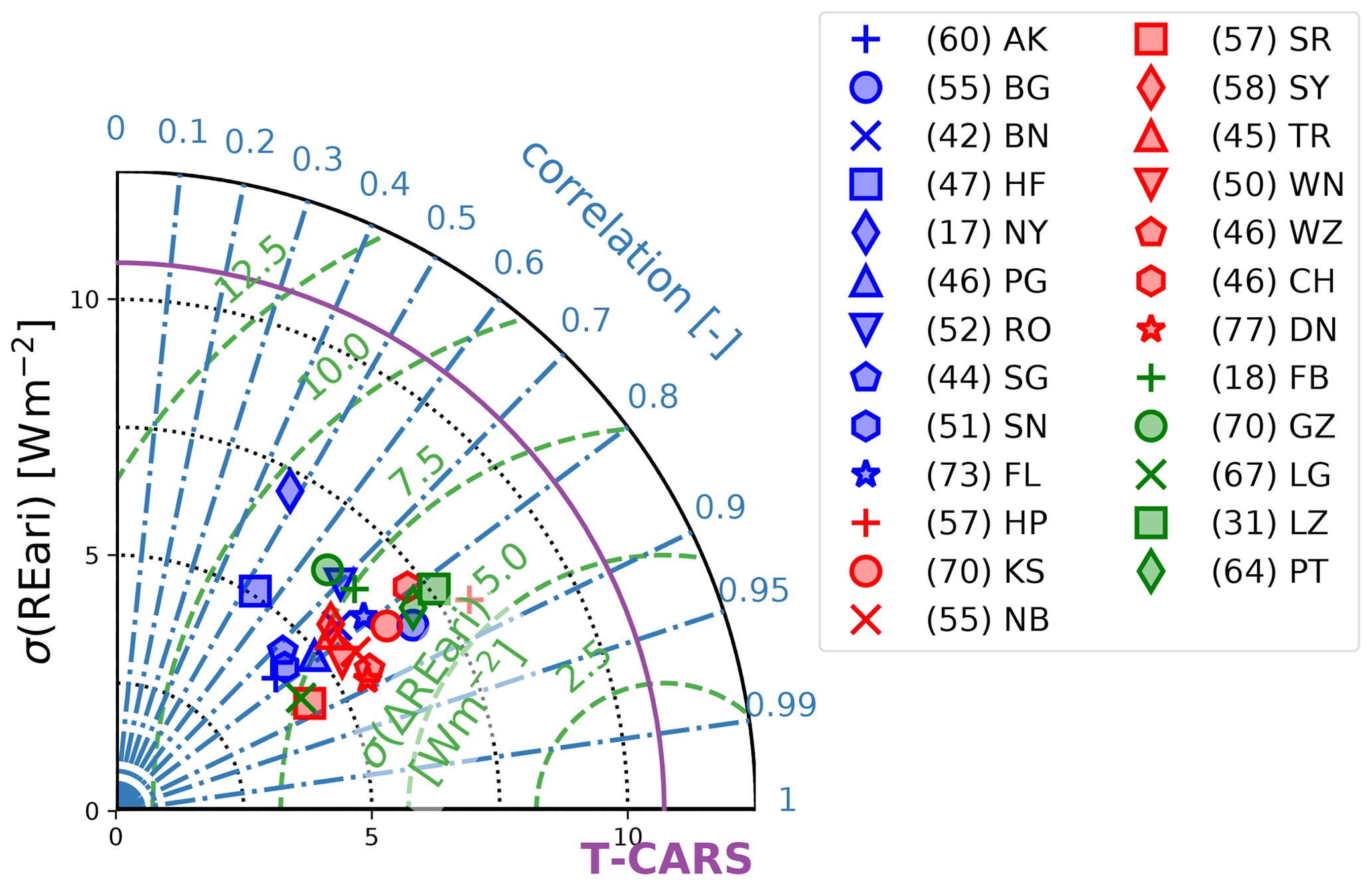
Figure 10The REari simulated at different DWD observation stations as the average over all CSM is compared to the collocated T–CARS simulation. The annual variability is indicated by the standard deviation (σ) of the individual dataset. The performance of REari calculated at a station is displayed by the SD of the REari difference and correlation versus T–CARS. The amount of days with a successful clear-sky fit are displayed in brackets in front of the station name in the legend. Station markers are colour coded based on their location labels (see Table 1): northern stations (blue), southern stations (red) and remaining stations (green).
Another Taylor diagram is shown in Fig. 10. Here, the average REari values retrieved from the CSMs are shown for each of the 25 DWD stations. This reveals regional performance differences of the observation-based approach versus T–CARS. The stations are separated in northern stations (blue), southern stations (red) and the remaining stations (green). At most stations, the REari values from CSM and T–CARS agree, having a correlation above 0.8. A correlation below 0.8 is mainly found for northern and coastal stations. This may have several reasons. On the one hand, T–CARS uncertainty in the northern region is increased due to lower incident radiation as shown by Fig. D2 and also due to lower aerosol absorption in this region, since CAMS RA tends to underestimate SSA (see Sect. 4.1.1). On the other hand, also the uncertainty of irradiance observations increases due to the lower sun elevation. The CSMs rely on their fixed empirical assumptions. Therefore, these models are limited in their representation of a pristine atmosphere. Especially for northern stations, the irradiance of a pristine atmosphere simulated by the CSM is close to the observed irradiance, leading to an underestimation of REari magnitude. The quality of the comparison statistics is also limited by the number of available measurements. The number of successful clear-sky fits used to estimate REari is shown in the legend of Fig. 10. This number varies between 17 and 75.
Based on the retrieval of REari from the irradiance observations using the different CSMs, the annual-mean value of REari for Germany and the year 2015 is quantified to be −13.2 ± 5.5 W m−2. This indicates that the set of CSM selected for this study enables an estimate of REari which is consistent with the collocated T–CARS simulations, which yield a value of REari of −11.4 W m−2. However, the annual variability of REari is underestimated, leading to an overestimation of REari in winter and an underestimation during summer. Only the ESRA and CEM models are able to reproduce a realistic annual cycle of REari, while the CEM largely overestimates the REari magnitude. From the set of chosen CSM, the ESRA, MRM v6.1, Heliosat-1 and Solis simple models show the highest level of agreement of the annual-mean REari, lying in the range of −11.1 to −15.2 W m−2. With the ESRA model, the annual cycle of REari was reproduced with a reasonable correlation of 0.77. The annual mean of REari retrieved with Heliosat-1 agrees best with T–CARS, with an MBE of −0.1.
Compared to the CSM performance ranking given by Sun et al. (2019) (see Table 9), the ESRA model which performs best in this study has the worst score in Sun et al. (2019). Since the CSMs were not designed to retrieve AOD or the REari, this performance discrepancy is not surprising. Since the analysis in this study is based on 1 year of data only, the representativity of our results may be limited.
In general, the retrieval of REari from observations is limited by the availability of clear-sky observations, and the number of suitable days is small in the mid-latitudes. Also, the retrieved REari strongly depends on the individual assumptions and definitions used by the CSM, which are also not tuned for the German region explicitly. The representation of the pristine irradiance in the CSMs directly influences the accuracy of the simulated REari. The constant aerosol properties in the models limit their ability to reproduce the REari variation during the annual cycle. Therefore, this approach cannot be recommended for climatological studies but may provide valuable information for case studies, e.g. for the evaluation of power generation and the influence of aerosols on photo-voltaic power plants.
4.3 Aerosol optical properties and REari over Germany
In this section, the hypothetical radiation budget, excluding clouds, and the REari over the region of Germany for the year 2015 are analysed. For this purpose, the clear-sky irradiance and REari as simulated with the T–CARS setup are used as basis, and a bias correction has been applied based on the results of the uncertainty analysis described in Sect. 4.1.3.
The considered region covers a domain from 47 to 55∘ N and from 6 to 15∘ E including parts of Central Europe (see Fig. 2). In the north, this domain includes parts of the coastal regions of the north and Baltic Sea. In the south, it covers the mountainous region of the northern Alps. The north-western part is dominated by a temperate oceanic climate (Cfb) and the south-eastern part by a humid continental climate with warm summers (Dfb) according to Beck et al. (2018). Some individual regions at higher altitudes are designated as colder subarctic climate (Dfc).
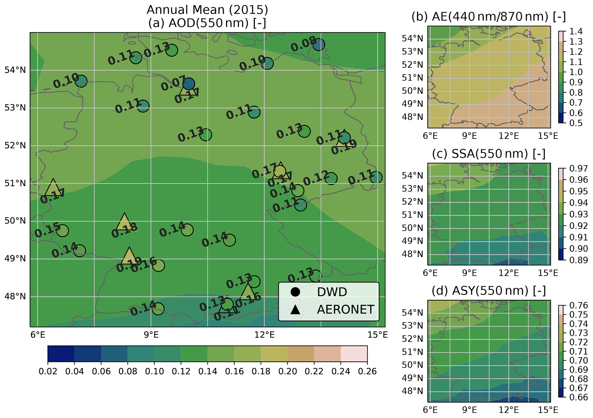
Figure 11Annual mean of aerosol properties at the surface over Germany. The calculation is conducted with the T–CARS setup. In addition for the AOD (a), annual-mean values as observed from measurement stations from AERONET (triangles) and DWD (circles) are shown. Note that considerable differences between T–CARS and measurement stations may be attributed due to sampling effects on the estimation of the annual mean, localized intense sources of aerosol (inner cities) and terrain inhomogeneity (e.g. Gueymard and Yang, 2020).
An overview of the annual-mean aerosol properties over Germany is shown in Fig. 11, considering AOD, AE, SSA and ASY. Low AOD values are found in the southern regions, especially at higher altitudes, while the AOD is largest in the northern and eastern parts of Germany. Aerosol absorption increases towards the south-east, as shown by lower SSA values. As expected, the south-eastern regions are also characterized by larger AE values, which indicate a more continental aerosol with a higher fine-mode fraction. Stronger forward scattering is indicated by larger values of the ASY in the north, which is attributable to the strong forward-scattering properties of sea salt (Bozzo et al., 2020a). These general patterns are similar for all seasons (see Appendix D, Figs. D4 to D7). The seasonal cycle is characterized by higher average values of AOD and AE in summer and lower values in winter.
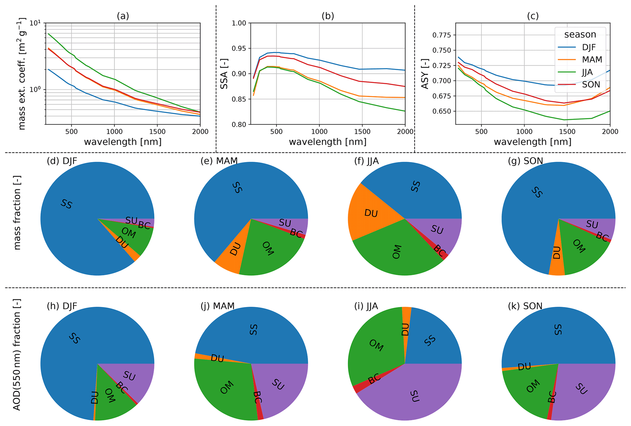
Figure 12Seasonal mean of the mass extinction coefficient, single scattering albedo (SSA) and asymmetry parameter (ASY) (a–c) of the aerosol mixture (d–g) and (h–k) from the CAMS RA aerosol properties database over Germany 2015. The aerosol mixture pie charts show the column-integrated mass fraction of each aerosol classification (d–g) (see Bozzo et al., 2020a) and the contribution to the extinction by fraction of AOD at 550 nm (h–k) (SS – sea salt; DU – mineral dust; OM – organic matter; BC – black carbon; SU – ammonium sulfate).
Figure 12 shows the seasonally averaged optical properties of the aerosol mixture from CAMS RA together with the mass fraction of each aerosol type contributing to the overall mixture. Sea salt is the dominant component, followed by organic matter, which becomes larger in summer. Except for summer, the fraction of mineral dust, sulfate and black carbon lies below 10 %, while these three aerosol classes make up 25 % of the aerosol mixture in summer. This causes an increased aerosol absorption in summer in combination with larger values of AOD. In winter, sea salt contributes more than 80 % to the aerosol mixture, which leads to lower values of absorption and AOD.
While the radiative transfer simulations made with the T–CARS scheme consider all 60 model layers available from CAMS RA, REari is only calculated and discussed for the surface and the TOA here.
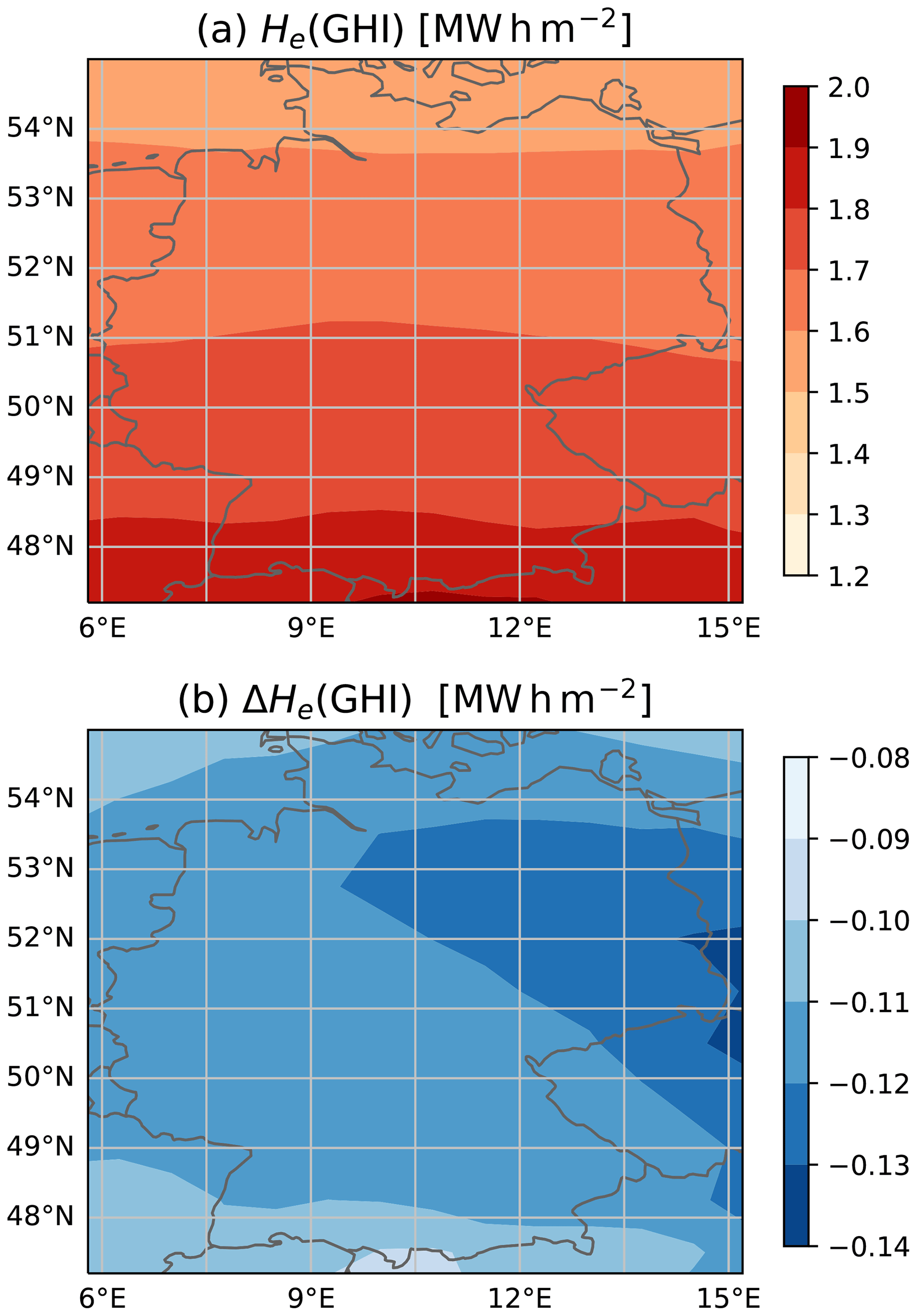
Figure 13Annual radiant exposure () computed from GHI assuming cloud-free conditions (a) and reduction due to aerosols (, b) at the surface over Germany in 2015. The calculation is conducted with the T–CARS setup.
The daily average surface irradiance increases towards the south due to the higher average sun elevation. Furthermore, a tendency of more frequent clear-sky situations towards the south exists. This is reflected in the accumulated hours of sunshine duration (see Fig. 2 and Table 1) and causes an increased average irradiance during the considered year in the south. The radiant exposure for Germany is shown in Fig. 13. It increases from north to south from 1 to 2 MW h m−2. Figure 13 also shows the reduction of the radiant exposure by aerosols. The reduction of GHI shows values in the range from −0.14 to −0.08 MW h m−2. The reduction of the radiant exposure calculated from GHI seems to be dominated by aerosol absorption. The strongest GHI reduction by aerosols is shown for the south-east, where aerosols are characterized by continental sources with larger absorption values. For comparison, the radiant exposure due to the contribution of the direct irradiance on a horizontal plane (μ0DNI) is also shown in Appendix D in Fig. D8. Similar patterns are evident here, despite the fact that the DNI is influenced more strongly by aerosols. The spatial pattern of the direct irradiance follows that of the AOD shown in Fig. 11 but is also increased by the larger incident radiation in the south.
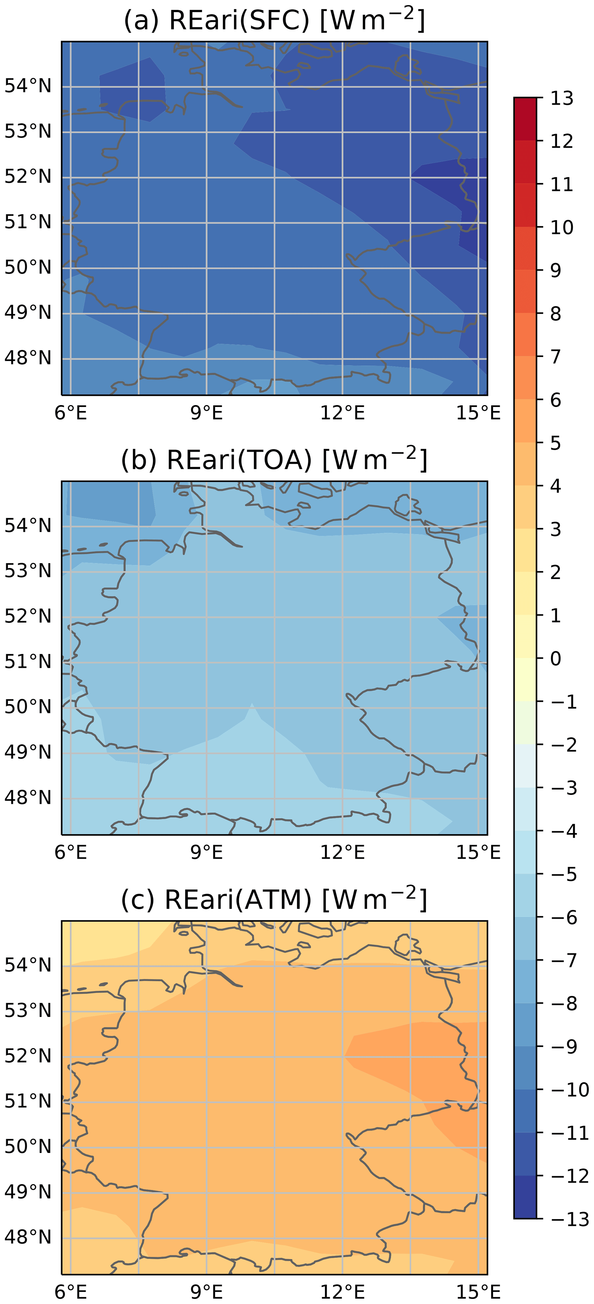
Figure 14Annual-mean REari at the surface (SFC), TOA and total atmosphere (ATM) over Germany. The simulation is conducted with the T–CARS setup.
The spatial distribution of the annual-mean REari in 2015 at the surface, TOA and for the total atmosphere simulated by T–CARS is presented in Fig. 14. The annual-mean values of REari over Germany 2015 vary regionally between −13 and −8 W m−2 at the surface and between −9 to −5 W m−2 at the TOA, where maximum absolute values are shown in the south-eastern region, following the spatial pattern of irradiance reduction shown in Fig. 13. Aerosols contribute to atmospheric heating in general over Germany, as the magnitude of the annual-mean REari at the TOA is always smaller than REari at the surface, and therefore the REari for the total atmosphere remains positive. The magnitude of REari at the surface and TOA is generally larger towards the east due to higher values of aerosol absorption (see Figs. 11 and 13). Stronger incident radiation increases the REari towards the south, but due to higher altitudes and reduced aerosol concentration, surface REari shows lower values in the southern region.
Table 10Annual and seasonal mean of the REari over Germany (47 to 55∘ N and 6 to 15∘ E) quantified by T–CARS.
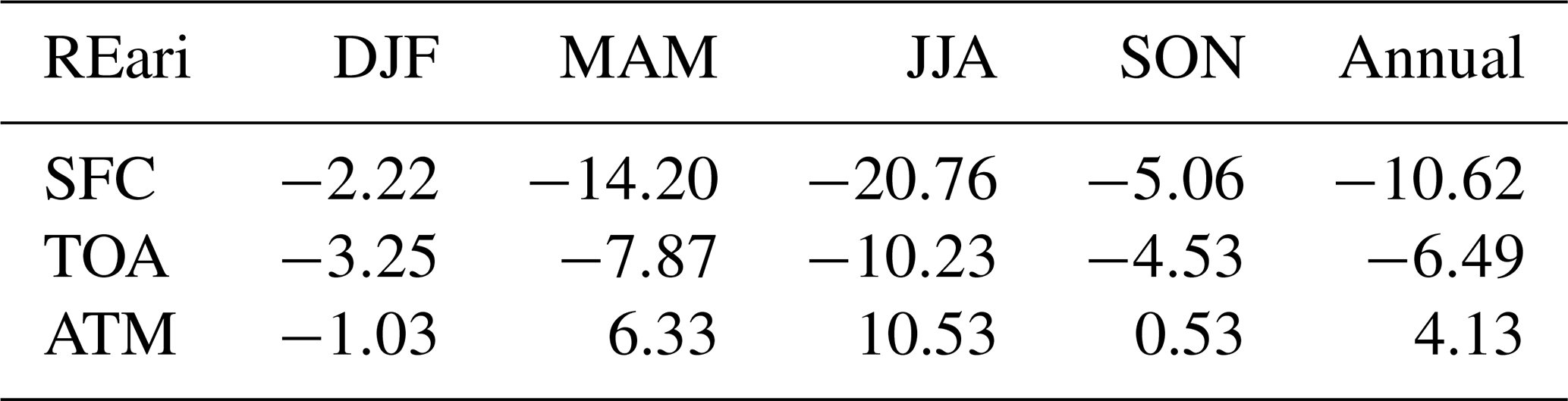
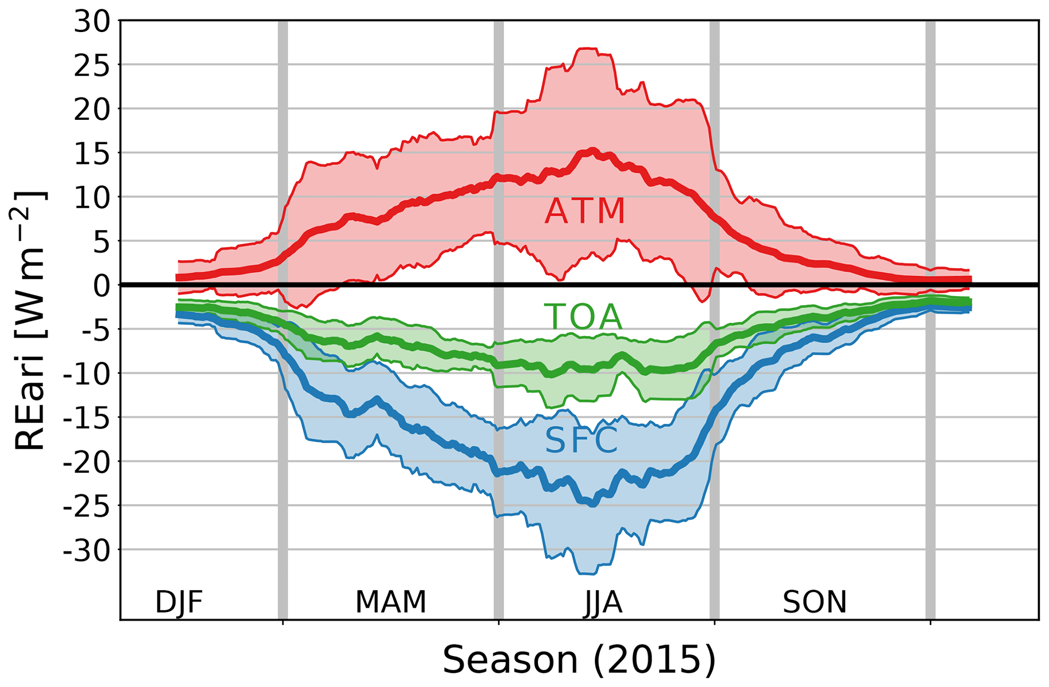
Figure 15The 30 d rolling mean of REari at the surface (SFC), top of the atmosphere (TOA) and total atmosphere (ATM) of the year 2015 simulated with T–CARS over Germany. The variability within 30 d is shown by the rolling SD as shaded areas.
Spatially averaged values of REari are summarized as seasonal and annual means in Table 10. The magnitude of all REari components increases from winter to summer. The annual cycle of REari is also shown in Fig. 15. As the REari values vary strongly on a daily basis due to changing weather and aerosol conditions, the REari values are smoothed by a 30 d rolling mean to highlight the general form of the annual cycle shown in this figure. Also shown is the variability of the REari expressed by the 30 d running standard deviation. The surface REari varies over the year from a value about −3 W m−2 in winter up to −25 W m−2 in summer. This increase in magnitude is expected due to the larger incident radiation and AOD values (see Fig. 12) during summer. During spring and summer, the REari magnitude at the TOA is always significantly smaller than at the surface, indicating significant atmospheric warming by aerosol. During fall and winter, REari values at the TOA and surface are nearly equal, which suggests that atmospheric warming due to aerosols is small or even zero.
The values of REari simulated with T–CARS for the German region are comparable to previous studies which have investigated the REari for the European region. Bartók (2016) quantified the annual-mean REari at the surface for the European region utilizing radiative transfer modelling (Mesoscale Atmospheric Global Irradiance Code, MAGIC) based on an aerosol (Kinne et al., 2006) and water vapour climatology (Dee et al., 2011). For the year 2005, Bartók (2016) found a similar pattern of the annual cycle of REari at the surface as shown in the present study (see Fig. 15). Values ranging from −14 W m−2 in summer to −3 W m−2 in winter and with an annual mean of −7.1 ± 2.9 W m−2 were given. Esteve et al. (2016) utilized a different radiation scheme (ES96) together with aircraft measurements of aerosol optical properties made during the EUCAARI-LONGREX campaign. The flights were conducted in May 2008 over Europe. Their results show values of −11 ± 5 W m−2 at the surface and −5 ± 3 W m−2 at the TOA. In the current study, higher values of REari at the surface and TOA of May 2015 are −17 ± 5 and −9 ± 3 W m−2, respectively.
Compared to Bartók (2016), the magnitude of the clear-sky REari calculated in this study is considerably larger (−10.6 W m−2). This might be a result of the different regions of interest. While Bartók (2016) quantified REari for the entire European region, spanning latitudes from 32 to 73∘ N and longitudes from −25 to about 35∘ E, the present study is focused only on the region over Germany (47 to 55∘ N and 6 to 15∘ E). For this subset, the values of REari at the surface from Bartók (2016) increase roughly to between −14 and −10 W m−2, in agreement with the present findings. Similar values over Germany have been found for the year 2005 by Kinne (2019) utilizing the Max Planck Aerosol Climatology version 2 (MACv2). Furthermore, Bartók (2016) proposed a trend of about −4.4 W m−2 per decade for the REari at the surface. Applying this trend to their results from the year 2005, an annual mean of −11.5 W m−2 is expected for the entire European region, which is slightly larger than the results obtained with T–CARS in this study.
In this study, the clear-sky REari at the surface has been investigated for the region of Germany (47 to 55∘ N and 6 to 15∘ E) and the year 2015 based on two different approaches.
First, clear-sky irradiance observations from the DWD station network have been utilized together with seven CSMs to retrieve the REari at 25 stations across Germany. This approach relies on a combination of a clear-sky detection and fitting technique and the subsequent use of the CSMs to quantify the aerosol effect on the solar surface irradiance components. Second, explicit radiative transfer simulations have been conducted with the T–CARS setup using aerosol and atmospheric properties from the CAMS RA as input to the ecRad radiation scheme. Given the fundamental differences of these two approaches, the consistency of the underlying aerosol properties and the resulting REari have been analysed and discussed.
The accuracy of the aerosol optical properties calculated from CAMS RA has been evaluated by a comparison to the version 3 direct sun and inversion products from AERONET observations as reference. The instantaneous values of CAMS RA AOD at 550 nm show a relatively large uncertainty of ± 0.09 and a correlation of 0.66, compared to the median value of 0.13. While the overall bias is nearly negligible, an increasing underestimation of larger AOD values and a slight overestimation of about 0.02 for AOD values below 0.1 have been observed. The level of agreement of the AE calculated from the CAMS RA AOD suffers from its limitation to values below 1.6 and a positive bias for AE values below 1. As a consequence, the representation of the spectral AOD is distorted depending on the aerosol type, which will mainly affect mineral dust (low AE) and aerosols with a strong spectral dependency of AOD (e.g. continental aerosol). The evaluation results for AOD and AE generally agree with previous studies (e.g. Inness et al., 2019a; Gueymard and Yang, 2020). To our knowledge, this is the first study to evaluate the intrinsic aerosol properties SSA and ASY calculated from CAMS RA. A large inconsistency between CAMS RA and AERONET inversions is found for the SSA and reflected by a significant bias of −0.03, leading to a strong overestimation of aerosol absorption. The distribution of values of the ASY agrees comparatively well with the AERONET product, with an MBE of zero and an RMSE of 0.04. It has to be emphasized, however, that the instantaneous agreement of all intrinsic aerosol properties shows potential for improvement, based on correlation coefficients of 0.51, 0.13 and 0.33 for AE, SSA and ASY, respectively.
In addition, the sensitivity of the REari has been studied utilizing the radiative kernel method (Thorsen et al., 2020). The results show that the REari is most sensitive to changes in SSA, ASY and AOD, while variations in AE and other atmospheric parameters (e.g. H2O and O3 column amounts or the surface albedo) do not significantly modify the magnitude of REari. AOD and SSA have been identified as the main contributors to the uncertainty of the REari. Correcting for the biases noted versus AERONET products, the REari calculated with T–CARS has a bias of −1.5 W m−2 at the surface and of 0.6 W m−2 at the top of the atmosphere. The SSA is the dominating source of this bias, caused by the underestimation of SSA in the CAMS RA aerosol properties. The main contribution to the random uncertainty of the daily-mean REari is the AOD uncertainty of ± 0.09. The resulting uncertainty of daily-mean REari has been calculated to have values of ± 7.7 W m−2 at the surface and ± 3.5 W m−2 at the top of the atmosphere. This yields an uncertainty of about ± 8.5 W m−2 for the REari within the atmosphere.
The clear-sky irradiance simulations from T–CARS have been evaluated versus reference observations from the DWD station network. The results show a high level of agreement for all three irradiance components (DNI, GHI and DHI), with a very high correlation for GHI (R>0.997) and values above 0.9 for DHI and DNI under most conditions. Furthermore, the level of agreement is within the expected range of the measurement uncertainty, with an RMSE of about 5 % to 10 % compared to the reference observations. The simulations of DNI and DHI improve through the consideration of aerosol properties obtained from the CAMS RA, as the SD of simulated and observed irradiance is substantially reduced by 5 to 30 W m−2. Furthermore, lower agreement has been found for the winter seasons due to lower incident radiation and longer atmospheric path lengths. It has been found that the level of agreement is reduced for northern or coastal stations with less absorbing aerosol, likely due to the overestimation of aerosol absorption by the CAMS RA aerosol properties mentioned before.
The results of the simulation of clear-sky irradiance and REari from the T–CARS setup are compared to the CSM-based retrieval results. This comparison provides insights into the level of detail required to estimate REari for climatology studies. The REari retrieved from the CSMs is strongly dependent on the assumptions of optical properties of aerosols and atmospheric gases used in the models. In general, the CSMs have not been tuned for our specific application, which requires a realistic representation of REari. Nevertheless, most models show a high level of agreement compared to the T–CARS reference simulations under pristine conditions, with absolute values of the bias below 10 W m−2 and RMSE values below 8 %. An exception is found for the CEM model, where the GHI in pristine conditions is overestimated by about 7 % as ozone absorption is not taken into account. A bias of pristine irradiance will introduce a bias of opposite sign in the retrieved REari. Therefore, the magnitude of REari is overestimated by MRM v6.1, ESRA and most strongly by the CEM model. An underestimation is noted for the METSTAT model. To retrieve the REari with the CSMs, the AOD was adjusted to fit the predicted GHI to observations under clear-sky conditions. The retrieved AOD was also compared to the CAMS RA-based values used in T–CARS in order to determine their consistency. The results show that the models are unable to reproduce the annual cycle of AOD, due to their reliance on a single aerosol type. The best level of agreement was found for the ESRA, CEM and METSTAT models.
For REari, the value retrieved from the CSMs is able to reproduce the annual mean (−12.8 ± 5.5 W m−2) of the T–CARS simulation (−11 W m−2). However, the CSM-based time series do not realistically reproduce the annual cycle due to their assumption of a fixed aerosol type. The best performance is shown by the ESRA and MRM v6.1 models. For annual averages of the REari, an approach based on CSMs leads to reasonably accurate results for the ESRA, MRM v6.1 and Heliosat-1 models. However, such an approach cannot be recommended for the estimation of the REari on a daily basis, since the random and systematic uncertainties vary throughout the year. A limitation which should be noted is that the present analysis is based only on 1 year of observations. Hence, representativeness of the results reported here should be confirmed based on a longer time period. The estimation of REari from clear-sky irradiance observations using CSMs may provide valuable information for the evaluation of the impact of aerosols on the power generation of photo-voltaic power plants. If atmospheric reanalysis data and aerosol properties data are available, the use of explicit radiative transfer simulations is recommended, since this approach provides a more realistic representation of clear-sky irradiance and REari and also offers height-resolved information independent of surface observations.
Finally, the best estimate of REari for Central Europe and Germany has been presented using the T–CARS simulations as basis. The dominating contribution to the aerosol mixture over Germany is sea salt aerosol, followed by organic matter, whose contribution increases during summer. This is accompanied by increased values of AOD and lower values of SSA during summer, which also increases the magnitude of REari. This tendency is reinforced by higher sun elevations during summer. Throughout the year, REari varies between −3 and −25, −2 and −10, and 1 and 15 W m−2 for the surface, top of the atmosphere and total atmosphere, respectively. Spatially, the aerosol mixture becomes increasingly continental towards the south-east, which is associated with an increased AE and stronger absorption. The AOD also follows this pattern, with an exception of lower AOD values in the south associated with higher altitudes in the mountain regions. A similar pattern is also observed for the REari. The bias-corrected annual-mean values of REari are −10.6 W m−2 at the surface, −6.5 W m−2 at the top of the atmosphere and 4.1 W m−2 for the total atmosphere. These results are consistent with previous studies quantifying the radiative effects of aerosols globally and for the European region (e.g. Bartók, 2016; Kinne, 2019).
The present study is limited to observations from a 1-year period. In the future, this analysis will be extended by the consideration of the full time series of long-term measurements available from the DWD station network to support the findings of this study with more robust statistics. In addition, an expanded database will allow a more accurate selection of the CSM that is best suited to estimate the REari over Germany, depending on its choice of atmospheric and aerosol parameterizations. Optimization of an existing CSM or implementation of a new CSM optimized for Germany based on those analysed here will be considered. For this purpose, simulations by the T–CARS setup can be used as basis, investigating the choice of a suitable set of climatological aerosol optical properties, and will provide additional insights into the level of detail required to estimate REari for climatological studies. A model optimized in this way will provide valuable information for case studies at specific locations.
Apart from case studies, the analysis of the REari will be extended utilizing the full temporal range of available CAMS RA data (2003–2020 at the time of writing). This provides the possibility to investigate REari trends in climatological studies. Furthermore, this study could be extended by using additional aerosol products that separate fine- and coarse-mode aerosol (e.g. MODIS, AERONET). This allows climatological studies on REari separately for aerosol from natural and anthropogenic sources.
Due to the modular structure of the ecRad radiation scheme, it is possible to extend the present T–CARS setup with inputs of atmospheric and aerosol properties, e.g. from active and passive remote sensing observations. This will improve the accuracy of the aerosol inputs and can help to account for sub-grid scale effects not resolved by the CAMS RA dataset, in particular for simulations at specific locations. This way, the T–CARS setup can also provide additional information about the REari for case studies with special aerosol conditions such as wildfire smoke (e.g. Baars et al., 2019; Ohneiser et al., 2020) or desert dust (e.g. Ansmann et al., 2017; Toledano et al., 2019), which might not be well represented in the CAMS RA.
A further interesting extension is the development of an optimum-estimation framework for adjusting the CAMS RA aerosol properties to yield solar irradiance components consistent with observations. If successful, such a framework might even open up the opportunity to assimilate broadband irradiance observations into CAMS RA in the future.
The clear-sky models (CSM) used in this study utilize different parameterizations for atmospheric components such as aerosols, trace gases and Rayleigh scattering to simulate the global horizontal irradiance (FGHI), the diffuse horizontal irradiance (FDHI) and the direct normal irradiance (FDNI). These irradiance components are related as follows:
where μ0 denotes the cosine of the solar zenith angle. Table 2 lists definitions, assumptions and required inputs of the CSM used to quantify REari from irradiance observations.
A1 MRM v6.1
The meteorological radiation model (MRM) was originally at the National Observatory of Athens (NOA) and has undergone continuous improvements. The version of MRM used in this study is 6.1 (Kambezidis et al., 2017). The direct normal FDNI and diffuse irradiance FDHI are calculated as follows:
Transmittance is considered in this model for aerosol extinction (A), Rayleigh scattering (R), water vapour (W) and ozone (O) absorption, depending on air mass m. Further, the absorption of mixed gases (CO2, CO, N2O, CH4 and O2) is considered (TMG). Each gas is considered with an individual fixed column amount. To estimate TA and TAS to account for aerosol extinction and scattering, a lookup table approach is used. The lookup table is based on four aerosol classifications taken from the SMARTS 2.9.5 models (Gueymard, 2005), which include urban, maritime, desert dust and continental aerosol. The AOD at 550 nm as input is used to select the appropriate aerosol classification. The lookup table provides the aerosol SSA (ω0) and the effective forward-scattering coefficient fa based on Brine and Iqbal (1983).
A2 ESRA
ESRA is used as the abbreviation for the clear-sky model in the framework of the digital European Solar Radiation Atlas (Rigollier et al., 2000). In ESRA, the FDNI is calculated by
with ϵ the correction from solar eccentricity for the solar constant S0, m the optical air mass and τR the Rayleigh optical depth. The influence of aerosols, ozone and water vapour in the atmosphere is described in this equation by the Linke turbidity at an air mass of 2 (TL), which is the ratio of optical depth of the atmosphere to the optical depth of the dry atmosphere in pristine conditions (Louche et al., 1986). The AOD at 550 nm and water vapour column amount are considered as input for the TL calculation, while the ozone amount is fixed at 343 DU. The altitude (z) of the point of interest is considered in m including refraction correction and TL with
where p and p0 are the pressure at altitude and surface (p0 equals 1023.25 hPa), and zh equal to 8434.5 m is the scale height of the Rayleigh atmosphere near the earth's surface. The pressure ratio is used in TL, while the exponent of the altitude ratio is utilized for the calculation of m.
The diffuse horizontal irradiance (FDHI) also depends on TL:
with Trd the diffuse transmission function and solar zenith scaled with the diffuse angular function fd:
with A1, A2 and A3 indicating unitless coefficients which depend on TL. These coefficients are described in Rigollier et al. (2000).
A3 Heliosat-1
The Heliosat method for clear-sky irradiance estimation was developed to estimate the surface clear-sky irradiance from satellite images. In this paper the name Heliosat-1 is used for the method described in Hammer et al. (2003) following the naming in Sun et al. (2019).
The representation of the direct normal irradiance FDNI is equal to the calculation in the ESRA method (Sect. A2) with the exception that m is not corrected for solar refraction. The diffuse irradiance component FDHI is calculated using an empirical relation by Dumortier (1995):
The global irradiance is then calculated from the diffuse and direct component using Eq. (A1).
A4 Solis simple
The Solis model was developed within the framework of the Heliosat-3 project. It is a spectrally resolved physical model, based on radiative transfer calculation (Mueller et al., 2004):
where τb, τg and τd are the direct normal, global and diffuse optical depths, and b, g and d are the parameters obtained from radiative transfer calculations. For the use in real-time processes, a simplified version is presented by Ineichen (2008a). Based on a large set of simulations for altitude in the range of sea level to 7000 m, AOD at 700 nm from 0 to 0.45 and water vapour column from 0.2 cm to 10 cm, τb, τg, τd, b, g and d are parameterized. Ozone was taken as constant for the simulations at 340 DU. Trace gases in the atmosphere or surface albedo are not explicitly considered in this model.
A5 CEM
The CEM model was developed by Atwater and Ball (1978). The direct and global irradiance components are both calculated by the following equation:
where aW denotes the water vapour absorption and TR denotes the definitions of the Rayleigh and atmospheric transmission with individual coefficients for FDNI and FGHI, which depend on pressure and the air mass m formulation of Atwater and Ball (1978):
The global irradiance is scaled by a factor f, which depends on surface albedo a.
Following Gueymard (2003), the original formulation of the aerosol transmission based on Mie theory as described in Atwater and Brown (1974) is replaced by the Unsworth–Monteith turbidity coefficient depending on the broadband AOD (τA):
Since aerosol is considered in FGHI with TA only, extinction by aerosols is related to absorption only. Ozone is not considered in the CEM model.
A6 MMAC
The MAC model was originally developed by Davies and McKay (1982) and used in various forms in the literature. The direct normal irradiance FDNI is calculated by
Similar to CEM, aW denotes the water vapour absorptance, and transmittance T is considered for aerosol extinction (A), Rayleigh scattering (R) and ozone absorption (O). All parameters are dependent on relative air mass, which is formulated as in the CEM model (Eq. A16). This model was reviewed by Gueymard (1993), who concluded that the definition of aerosol transmittance TA degrades the performance of the model. In the modified MAC model (MMAC), TA is expressed equally to the CEM model (Eq. A17), following Gueymard (2003). Although very similar to the expression of FDNI in the CEM model, the MMAC model is considered for a climatological value of ozone and has a different parameterization of TR.
For the diffuse horizontal irradiance, Rayleigh scattering and scattering by aerosols are considered:
with broadband aerosol SSA ω0 equal to 0.98 and the ratio of forward to total scattering by aerosol f equal to about 0.1, following Sun et al. (2019).
A7 METSTAT
The meteorological and statistical solar radiation model (METSTAT) was developed for the production of the national solar radiation database of the United States (Maxwell, 1998). The clear-sky FDNI is calculated based on Bird's model (Bird and Hulstrom, 1981):
where transmittance T is considered for broadband Rayleigh scattering (R), absorption by ozone (O), water vapour (W), uniformly mixed gases (UM) and extinction by aerosols (A). Each transmittance is a function of air mass. TA is calculated similar to CEM (Eq. A17) but with a different formulation of air mass.
An empirical function is used to calculate the diffuse irradiance component FDHI. This involves assumptions of broadband aerosol SSA, which in this study equals 0.9. Further, the surface albedo is used to estimate the diffuse radiation from ground reflectance (Badescu et al., 2013).
Table B1List of acquired CAMS RA parameters for this study. The table keyword specifies if the parameter is acquired for the surface (sfc) or model level vertical column (ml).
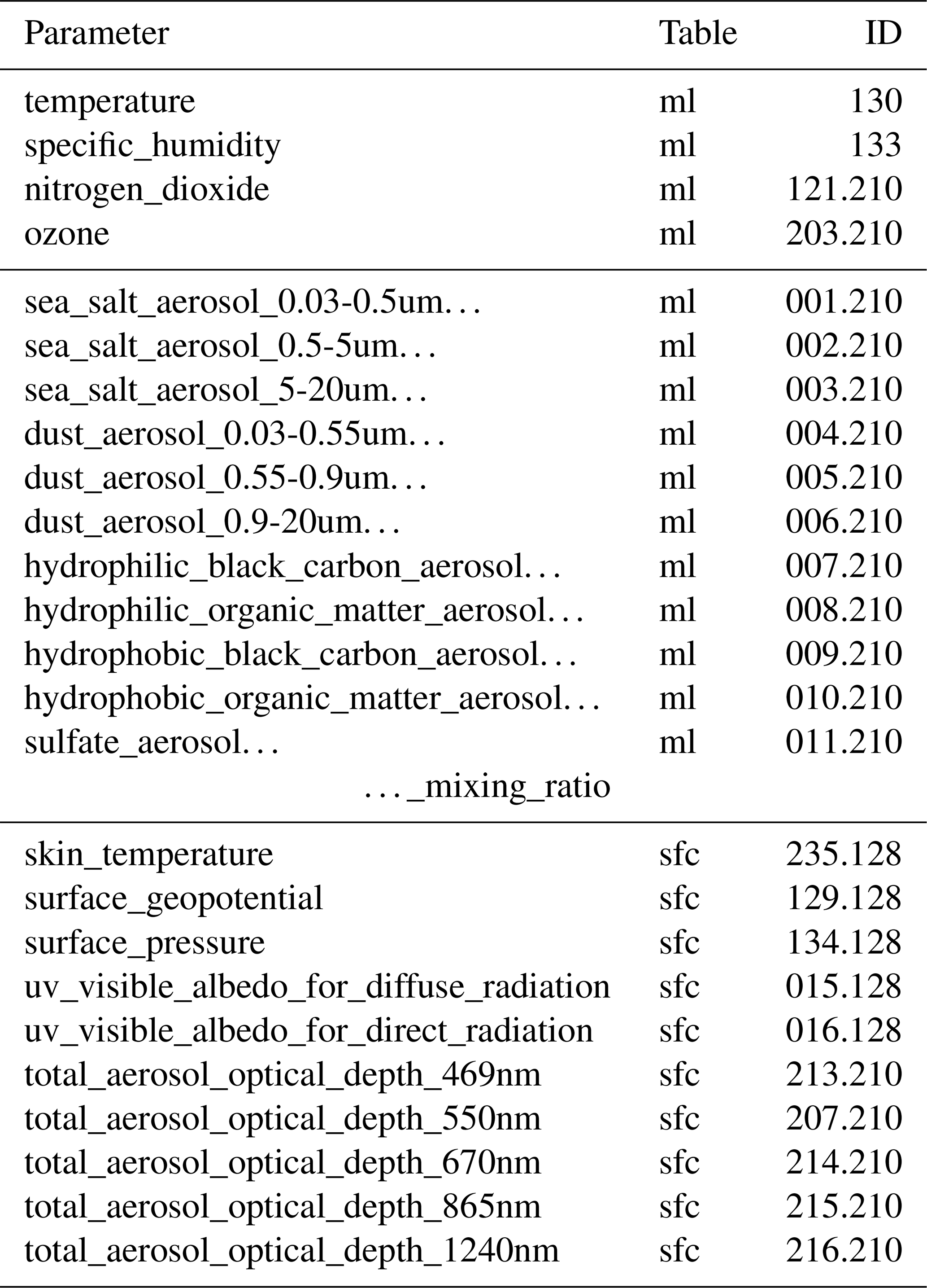
The aerosol properties in CAMS RA are given as mass mixing ratios (ri,l; see Table B1) for each of the 11 aerosol types (i) on 60 model levels (l). The aerosol optical properties' database described by Bozzo et al. (2020b) provides the mass extinction coefficient (aext,i), SSA and ASY for 20 monochromatic wavelengths in the range from 340 nm to 2130 nm as well as the ecRad bands and can be used for conversion to column-integrated values of AOD (τext,i), SSA (ωi) and ASY (gi) for a specific wavelength following Benedetti et al. (2009):
with Δpl denoting the pressure difference of bottom and top layer interfaces and g0 the standard gravity on earth of 9.80665 m s−2. A variation of g0 depending on latitude or altitude is not considered. Although not denoted here, all parameters except r, Δp and g0 are a function of spectral wavelength and humidity. In the database, the optical properties for hydrophilic aerosols are given in steps of 10 % humidity.
An REari estimate is provided by the AERONET inversion product, which is calculated from the downward fluxes only (oppositely to net fluxes as in this study); therefore, the surface albedo is neglected (Holben et al., 2006). As a consistency test, this REari product is compared with the T–CARS simulations. For this purpose, The T–CARS simulation collocated to the AERONET stations is calculated, setting the surface albedo to 0. Furthermore, as AERONET provides occasional observations during the day, the daily mean of observations are scaled to a daily average value using the ratio of collocated T–CARS simulations versus the daily average simulated by T–CARS. The comparison is shown in Fig. C1. In general, REari values calculated for both products agree with a correlation of 0.65 at the surface and 0.62 at the TOA. The MBE values indicate a stronger over- and underestimation of T–CARS REari as expected from the uncertainty estimate (Fig. 6), with values of −4.6 W m−2 at the surface and 5.6 W m−2 at the TOA. The MBE values found here are about 5 times larger than the theoretical uncertainty estimate based on the evaluation of the aerosol properties database (−1.5 W m−2 at the surface and 0.6 W m−2 at the TOA). The uncertainty estimate of REari shown above is based on the comparison to the aerosol properties products from AERONET. REari calculated by AERONET requires a set of assumptions about the state of the atmosphere (e.g. trace gases, vertical distribution, surface reflectance) which may be not consistent with the CAMS RA data. Therefore, these results deviate from the theoretical uncertainty estimate.
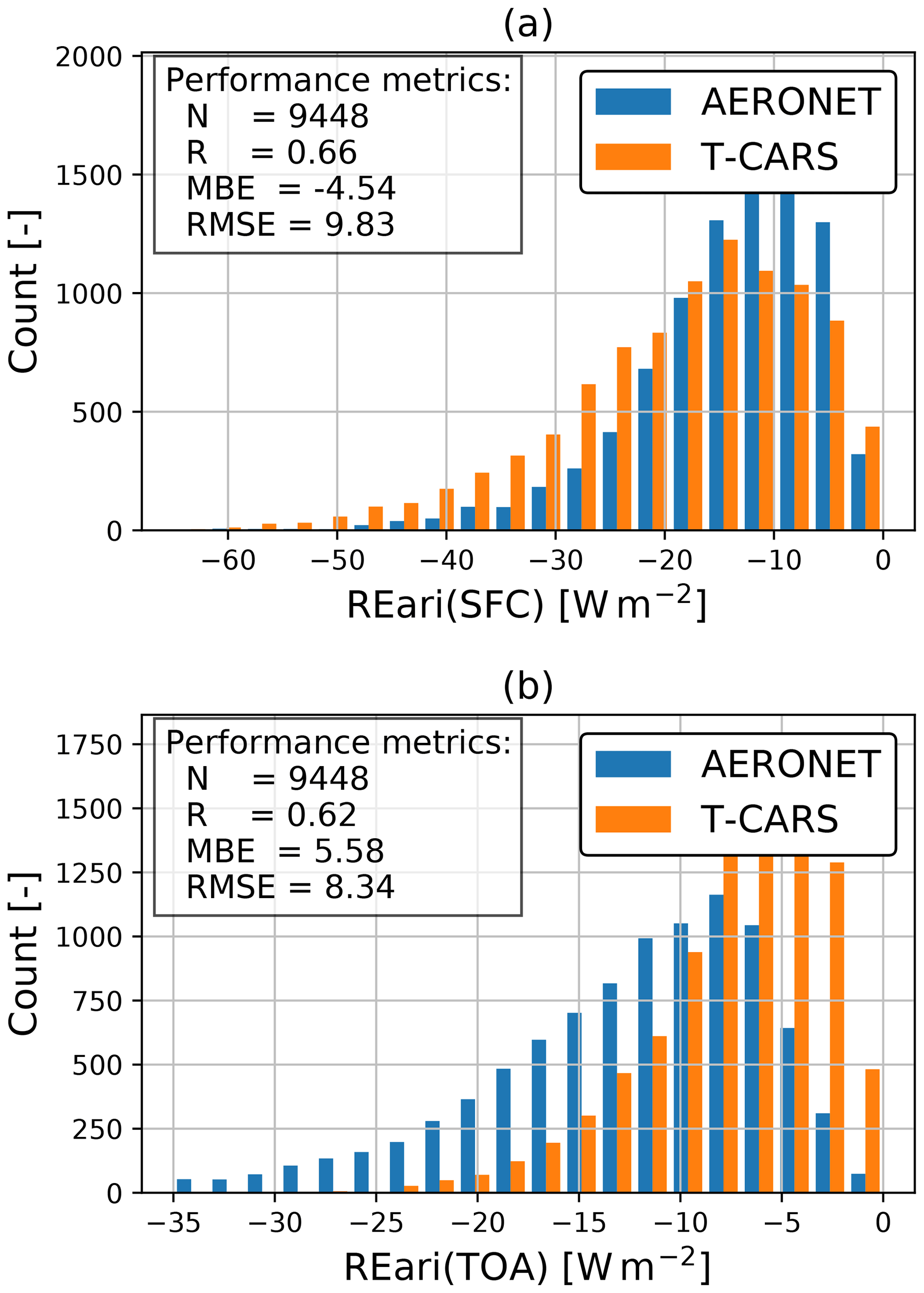
Figure C1Comparison of AERONET and T–CARS REari daily average products at the surface (SFC) and top of the atmosphere (TOA) for the period from 2003 to 2019. The metrics are calculated using the definition of REari (global instead of net irradiance at the surface) from AERONET and the AERONET data as reference.
Table D1Comparison of AOD provided by CAMS RA as reference and calculated with T–CARS from the CAMS RA model level aerosol mass mixing ratio. The data are acquired in the period from 2003 to 2019 for Germany.

Table D2As Table 1 but with the relative number of days for each season and the year 2015 to be interpolated for the results of Sect. 4.2.3 for each station (Figs. 7 and 8 Tables 8 and 9).
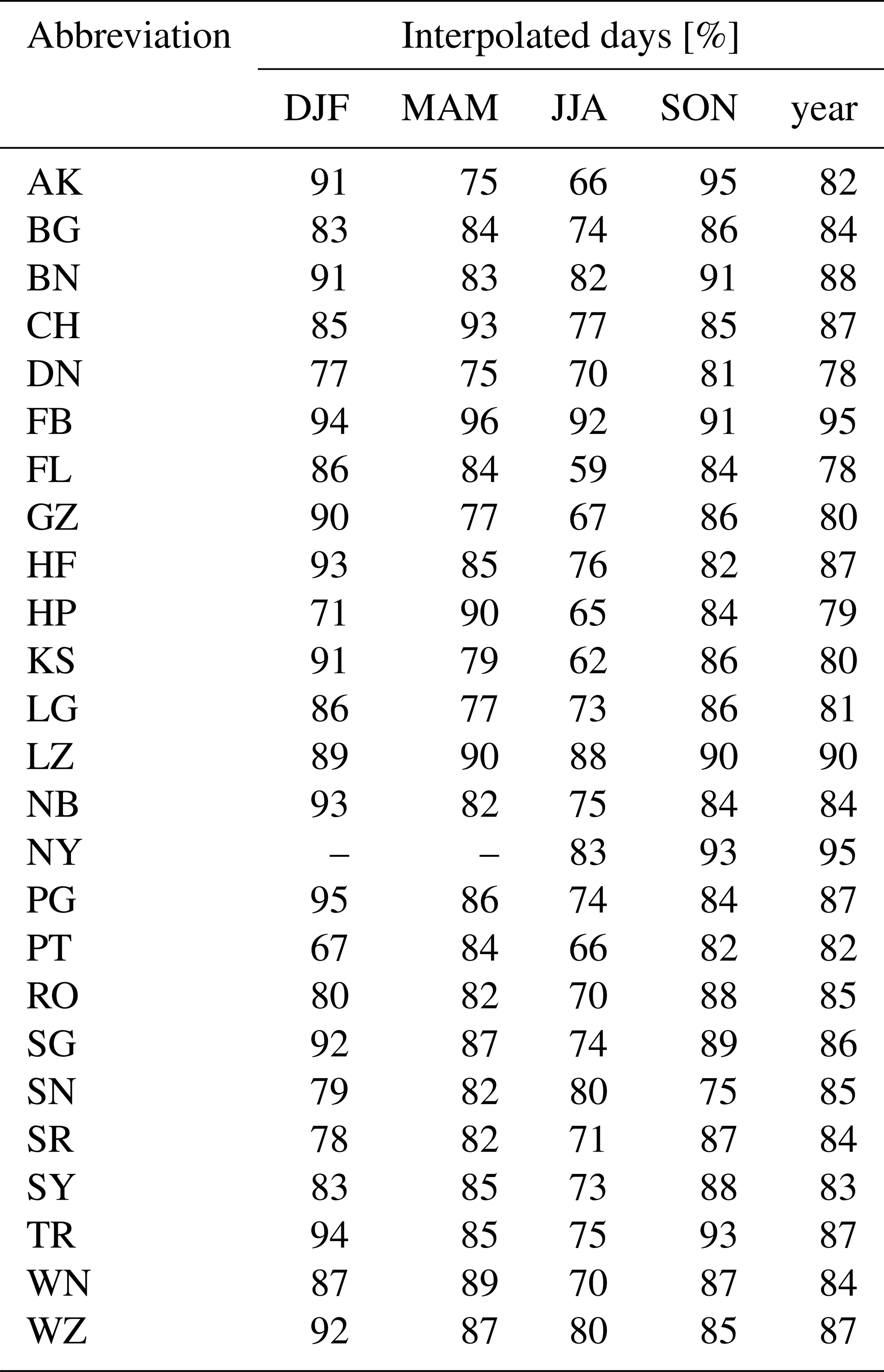
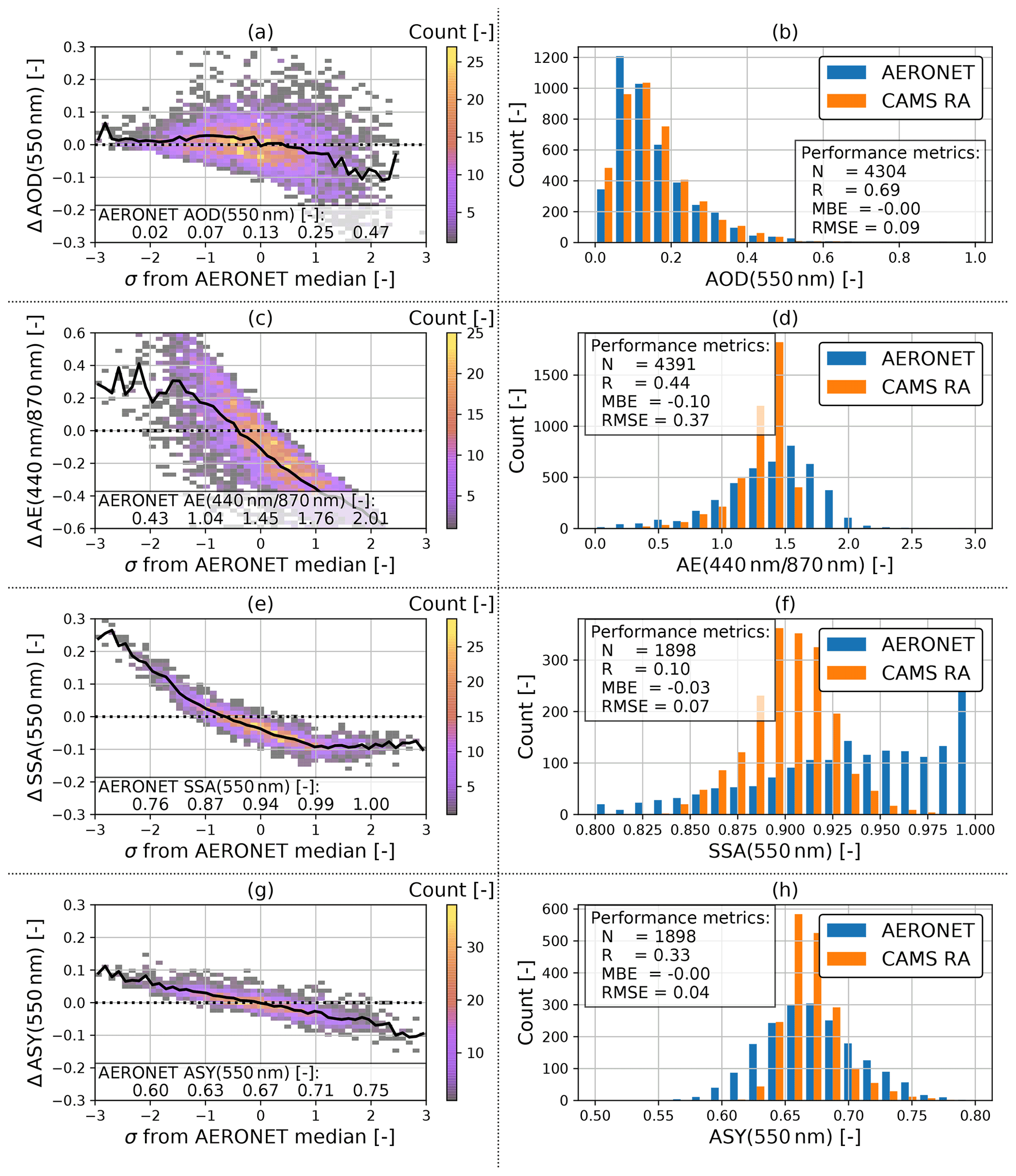
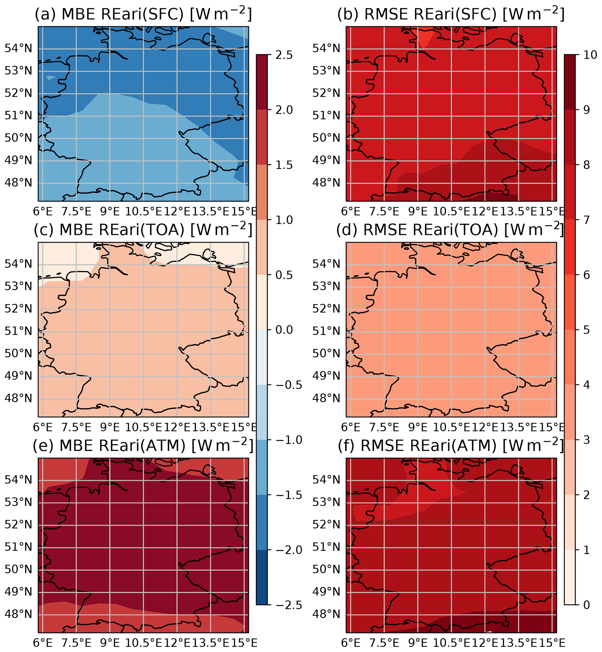
Figure D2Annual mean of REari MBE and RMSE of T–CARS over the region of Germany. The RMSE is calculated for daily average values of REari at the surface (SFC), top of the atmosphere (TOA) and for the total atmosphere (ATM).
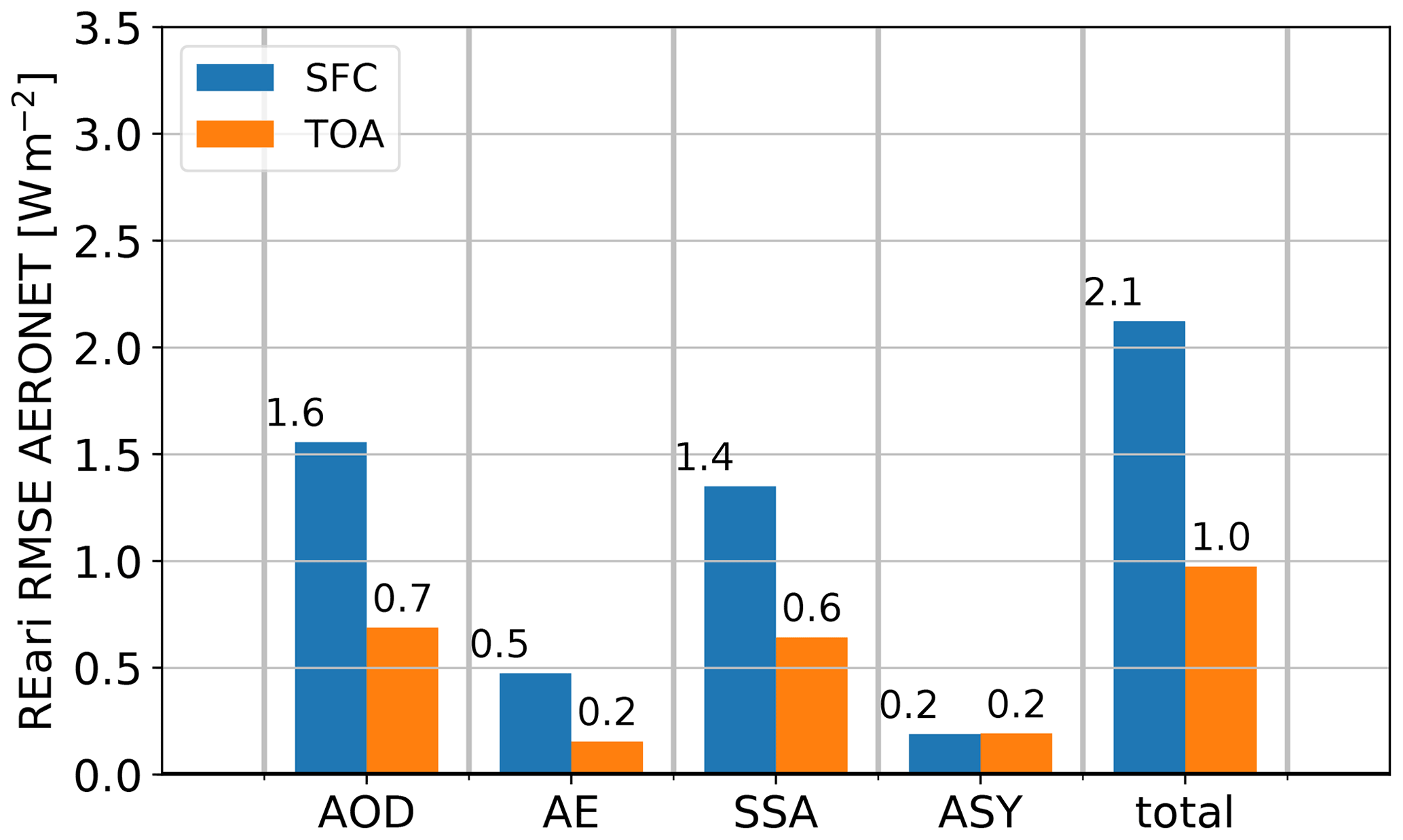
Figure D3REari kernels weighted by uncertainty estimates of AOD (± 0.02), AE (± 0.3), SSA (± 0.03) and ASY (± 0.01) from the AERONET direct and inversion products. The calculations are conducted for the surface (blue) and top of the atmosphere (orange).
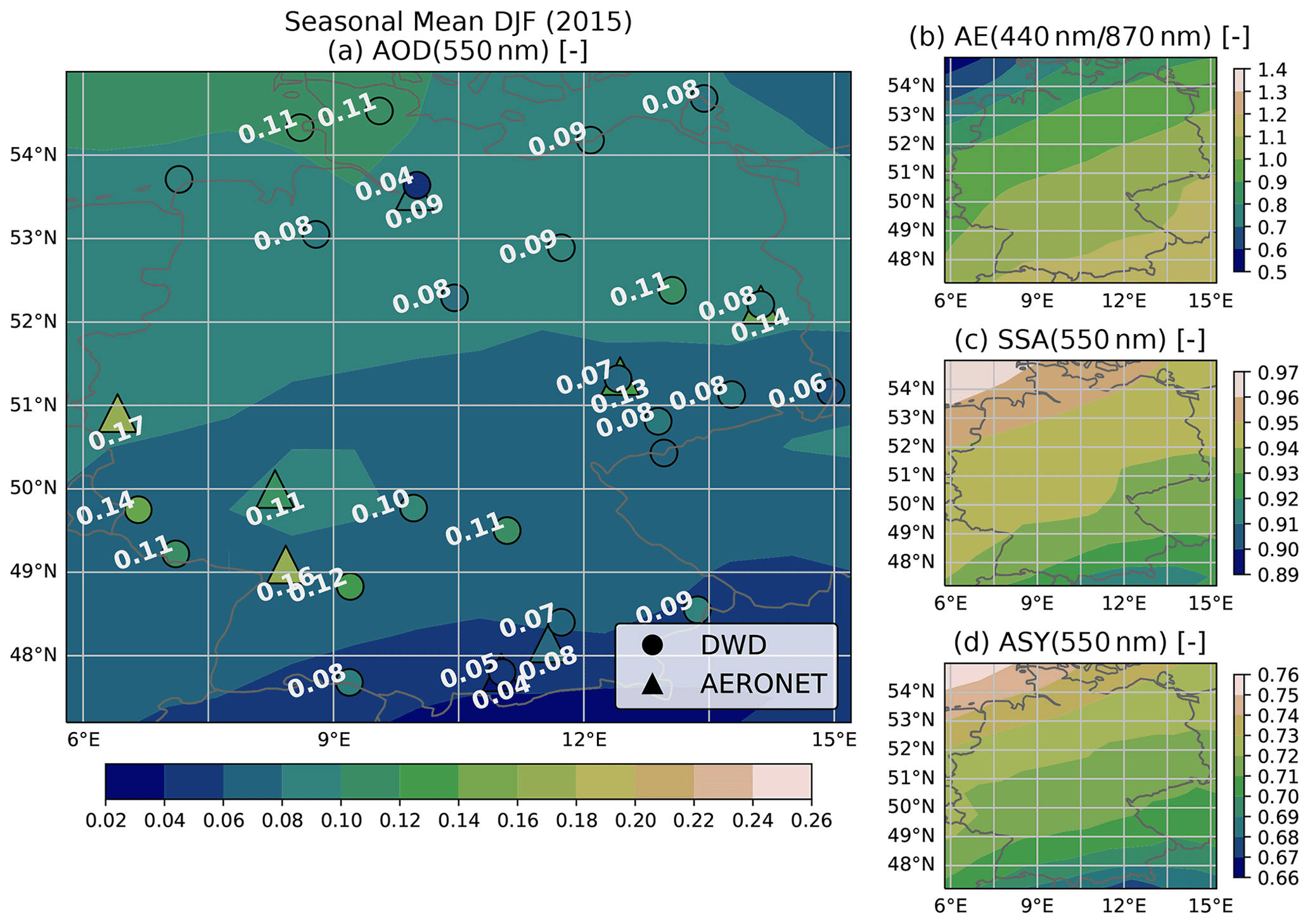
Figure D4As Fig. 11 but showing the average over winter 2015.
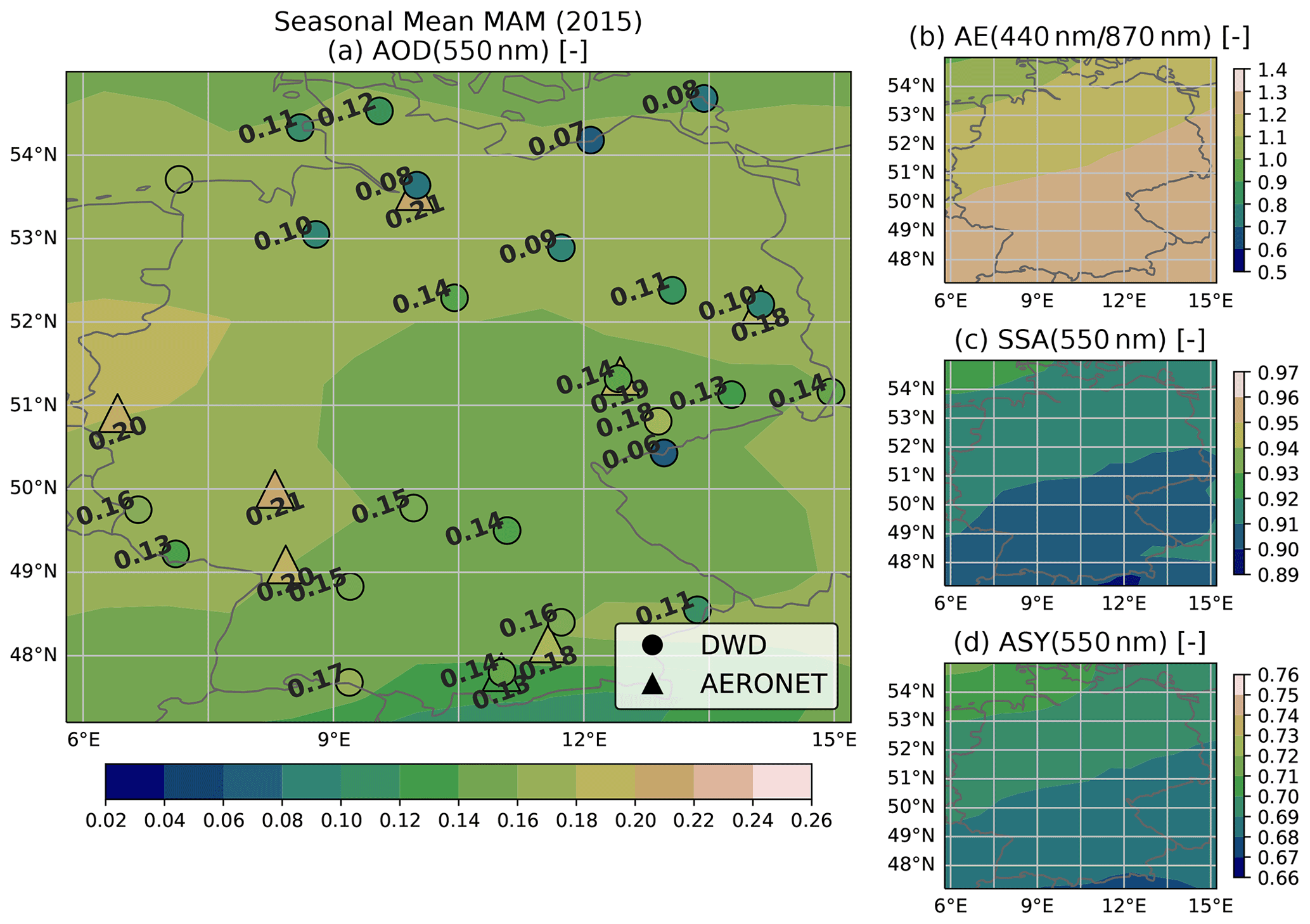
Figure D5As Fig. 11 but showing the average over spring 2015.
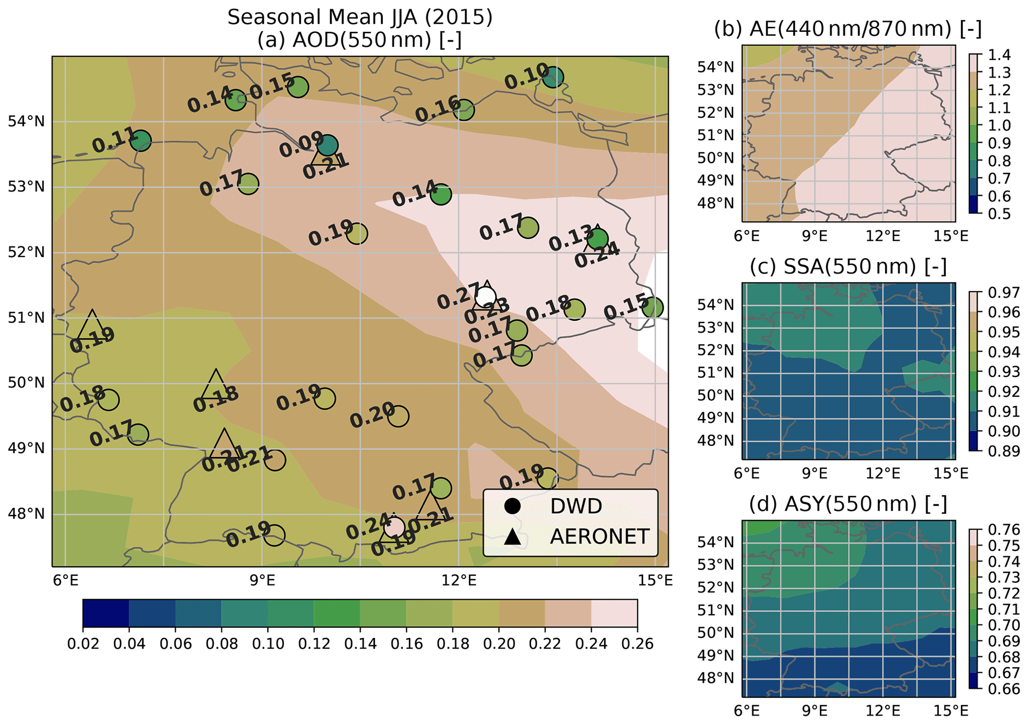
Figure D6As Fig. 11 but showing the average over summer 2015.
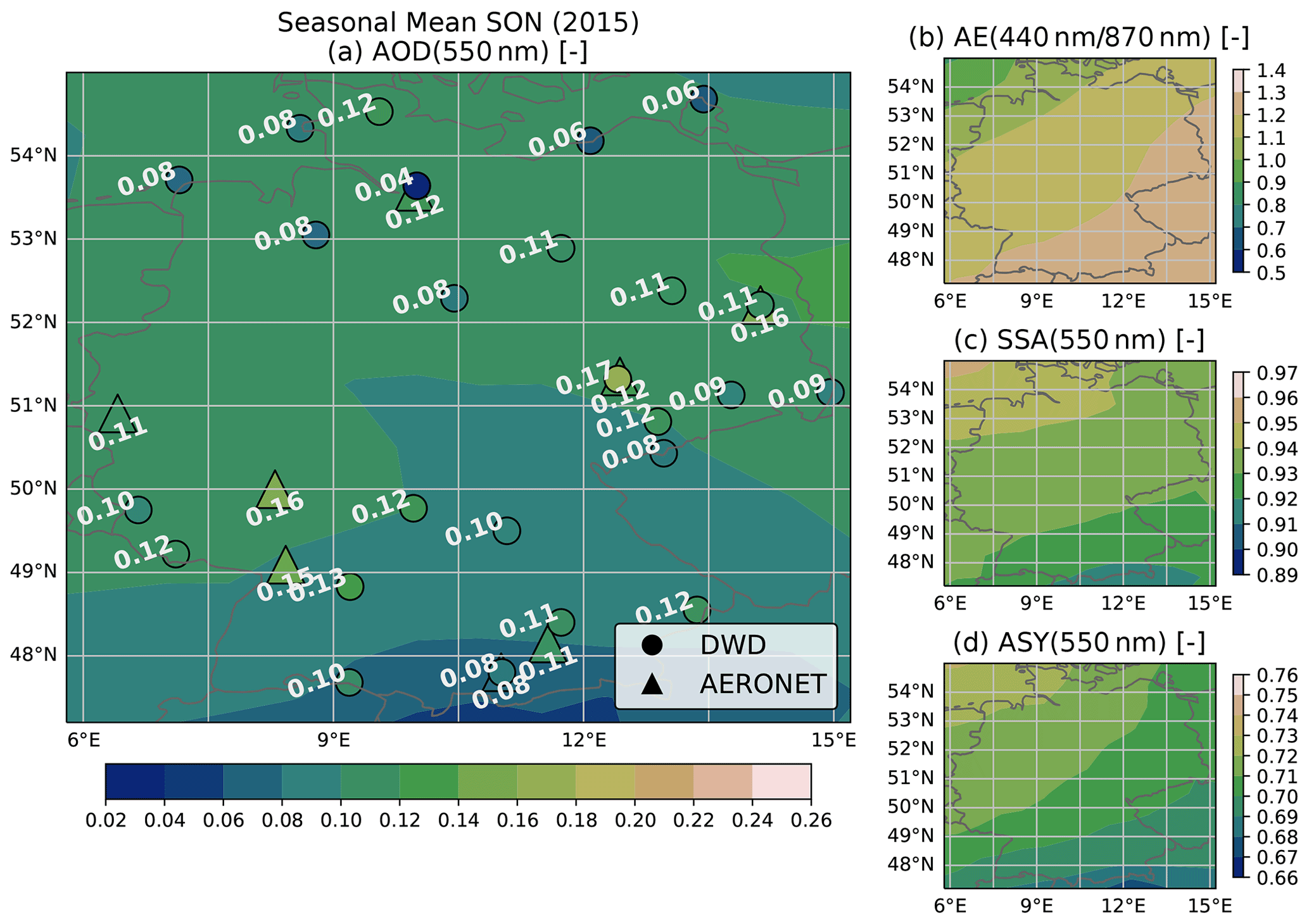
Figure D7As Fig. 11 but showing the average over fall 2015.
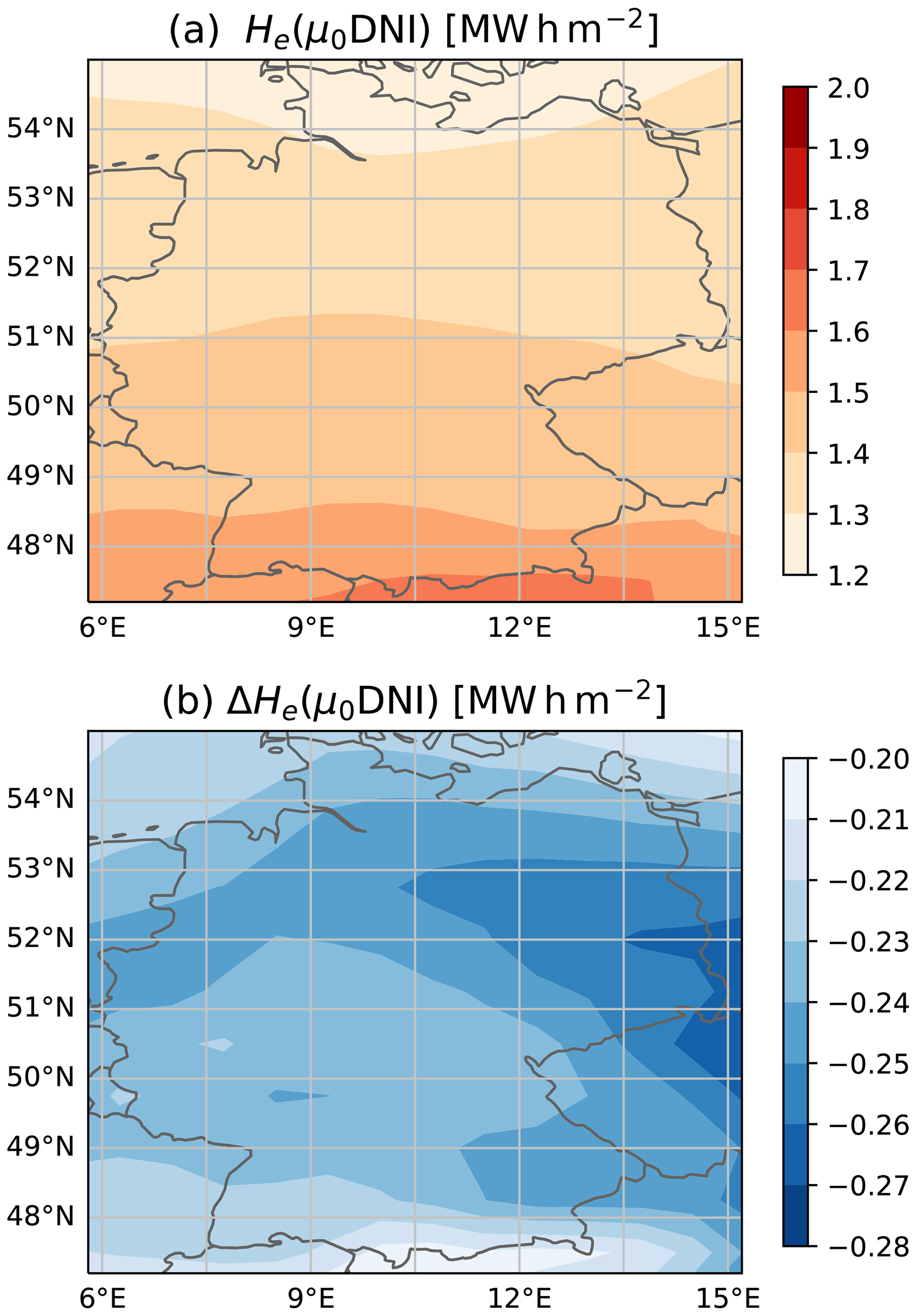
Figure D8Annual radiant exposure () from μ0DNI assuming cloud-free conditions (a) and reduction due to aerosols (, b) at the surface over Germany in 2015. The calculation is conducted with the T–CARS setup.
The code and data used are available from the repositories Witthuhn (2021) (https://doi.org/10.5281/zenodo.5347706) and Witthuhn et al. (2021) (https://doi.org/10.5281/ZENODO.4892729), respectively. With these, users can repeat the analysis presented in this study. Specific datasets and the source code were acquired from a variety of sources, listed as follows. The CAMS RA (CAMS global reanalysis EAC4) data can be downloaded from the Copernicus Atmosphere Monitoring Service (CAMS) Atmosphere Data Store (ADS) at https://ads.atmosphere.copernicus.eu (last access: 16 November 2020; Inness et al., 2019b). The data of the optical properties from CAMS RA, which is computed for each species for the 30 spectral band by the ECMWF radiation code and 20 single spectral wavelengths, are hosted on the CAMS data archive and available for download at https://doi.org/10.24380/jgs8-sc58 (Bozzo et al., 2020b). The AERONET version 3 direct sun and inversion products of aerosol optical properties are available at https://aeronet.gsfc.nasa.gov/ (Giles and Holben, 2021). The surface albedo utilized in the observational approach in this study was provided by the EUMETSAT Satellite Application Facility on Land Surface Analysis (LSA SAF; Trigo et al., 2011, http://lsa-saf.eumetsat.int). The offline version of the ecRad radiation scheme is available from ECMWF at https://github.com/ecmwf/ecrad (Hogan and Bozzo, 2018). The Bright–Sun clear-sky detection algorithm is available from GitHub at https://github.com/JamieMBright/csd-library (Bright et al., 2020). The algorithms of CSM utilized in this study are coded in the R language by Xixi Sun and collected by Jamie Bright in the GitHub repository at https://github.com/JamieMBright/clear-sky-models (Sun et al., 2019).
This work was conceptualized by JW and HD. The data were curated by JW, FF and SW. Formal analyses were conducted by JW and HD. Funding was acquired by HD and SM. JW led the research process and developed the methodology. The software for T–CARS was developed by JW. The work was supervised by HD and AH. JW prepared the manuscript with contributions from all co-authors.
The contact author has declared that neither they nor their co-authors have any competing interests.
Publisher’s note: Copernicus Publications remains neutral with regard to jurisdictional claims in published maps and institutional affiliations.
This paper contains modified Copernicus Atmosphere Monitoring Service information (2020); neither the European Commission nor ECMWF is responsible for any use that may be made of the information it contains.
For the aerosol product data from AERONET, we thank the principal investigators and co-investigators and their staff for establishing and maintaining the 25 sites used in this investigation.
Figures were plotted with the Python matplotlib package. Maps were plotted using the Cartopy library (Met Office, 2010–2015) and made with Natural Earth. Free vector and raster map data are available at https://naturalearthdata.com (last access: 30 September 2021). The labels on Fig. 2 were plotted using the Phlya/adjustText library for automatic text placement (Flyamer et al., 2018). Taylor diagrams were plotted utilizing the SkillMetrics package (Rochford, 2019).
The work presented in this paper has been conducted within the scope of the research project MetPVNet.
This research has been supported by the Bundesministerium für Wirtschaft und Energie (grant no. 0350009E).
This paper was edited by Stelios Kazadzis and reviewed by two anonymous referees.
Alia-Martinez, M., Antonanzas, J., Urraca, R., de Pison, F. J. M., and Antonanzas-Torres, F.: Benchmark of algorithms for solar clear-sky detection, J. Renew. Sustain. Ener., 8, 033703, https://doi.org/10.1063/1.4950948, 2016. a
Ansmann, A., Rittmeister, F., Engelmann, R., Basart, S., Jorba, O., Spyrou, C., Remy, S., Skupin, A., Baars, H., Seifert, P., Senf, F., and Kanitz, T.: Profiling of Saharan dust from the Caribbean to western Africa – Part 2: Shipborne lidar measurements versus forecasts, Atmos. Chem. Phys., 17, 14987–15006, https://doi.org/10.5194/acp-17-14987-2017, 2017. a
Atwater, M. A. and Ball, J. T.: A numerical solar radiation model based on standard meteorological observations, Sol. Energy, 21, 163–170, https://doi.org/10.1016/0038-092x(78)90018-x, 1978. a, b, c
Atwater, M. A. and Brown, P. S.: Numerical Computations of the Latitudinal Variation of Solar Radiation for an Atmosphere of Varying Opacity, J. Appl. Meteorol., 13, 289–297, https://doi.org/10.1175/1520-0450-13.2.289, 1974. a
Baars, H., Ansmann, A., Ohneiser, K., Haarig, M., Engelmann, R., Althausen, D., Hanssen, I., Gausa, M., Pietruczuk, A., Szkop, A., Stachlewska, I. S., Wang, D., Reichardt, J., Skupin, A., Mattis, I., Trickl, T., Vogelmann, H., Navas-Guzmán, F., Haefele, A., Acheson, K., Ruth, A. A., Tatarov, B., Müller, D., Hu, Q., Podvin, T., Goloub, P., Veselovskii, I., Pietras, C., Haeffelin, M., Fréville, P., Sicard, M., Comerón, A., Fernández García, A. J., Molero Menéndez, F., Córdoba-Jabonero, C., Guerrero-Rascado, J. L., Alados-Arboledas, L., Bortoli, D., Costa, M. J., Dionisi, D., Liberti, G. L., Wang, X., Sannino, A., Papagiannopoulos, N., Boselli, A., Mona, L., D'Amico, G., Romano, S., Perrone, M. R., Belegante, L., Nicolae, D., Grigorov, I., Gialitaki, A., Amiridis, V., Soupiona, O., Papayannis, A., Mamouri, R.-E., Nisantzi, A., Heese, B., Hofer, J., Schechner, Y. Y., Wandinger, U., and Pappalardo, G.: The unprecedented 2017–2018 stratospheric smoke event: decay phase and aerosol properties observed with the EARLINET, Atmos. Chem. Phys., 19, 15183–15198, https://doi.org/10.5194/acp-19-15183-2019, 2019. a
Badescu, V., Gueymard, C. A., Cheval, S., Oprea, C., Baciu, M., Dumitrescu, A., Iacobescu, F., Milos, I., and Rada, C.: Accuracy analysis for fifty-four clear-sky solar radiation models using routine hourly global irradiance measurements in Romania, Renew. Energ., 55, 85–103, https://doi.org/10.1016/j.renene.2012.11.037, 2013. a
Barlakas, V., Deneke, H., and Macke, A.: The sub-adiabatic model as a concept for evaluating the representation and radiative effects of low-level clouds in a high-resolution atmospheric model, Atmos. Chem. Phys., 20, 303–322, https://doi.org/10.5194/acp-20-303-2020, 2020. a
Bartók, B.: Aerosol radiative effects under clear skies over Europe and their changes in the period of 2001-2012, Int. J. Climatol., 37, 1901–1909, https://doi.org/10.1002/joc.4821, 2016. a, b, c, d, e, f, g, h, i
Beck, H. E., Zimmermann, N. E., McVicar, T. R., Vergopolan, N., Berg, A., and Wood, E. F.: Present and future Köppen-Geiger climate classification maps at 1-km resolution, Sci. Data, 5, 180214, https://doi.org/10.1038/sdata.2018.214, 2018. a, b, c
Becker, R. and Behrens, K.: Quality assessment of heterogeneous surface radiation network data, Adv. Sci. Res., 8, 93–97, https://doi.org/10.5194/asr-8-93-2012, 2012. a
Bellouin, N., Quaas, J., Morcrette, J.-J., and Boucher, O.: Estimates of aerosol radiative forcing from the MACC re-analysis, Atmos. Chem. Phys., 13, 2045–2062, https://doi.org/10.5194/acp-13-2045-2013, 2013. a
Benedetti, A., Morcrette, J.-J., Boucher, O., Dethof, A., Engelen, R. J., Fisher, M., Flentje, H., Huneeus, N., Jones, L., Kaiser, J. W., Kinne, S., Mangold, A., Razinger, M., Simmons, A. J., and Suttie, M.: Aerosol analysis and forecast in the European Centre for Medium-Range Weather Forecasts Integrated Forecast System: 2. Data assimilation, J. Geophys. Res., 114, D13205, https://doi.org/10.1029/2008jd011115, 2009. a
Bird, R. E. and Hulstrom, R. L.: Simplified Clear Sky Model for Direct and Diffuse Insolation on Horizontal Surfaces, techreport SERI/TR-642-761, Solar Energy Research Institute, available at: https://www.nrel.gov/grid/solar-resource/assets/data/tr-642-761.pdf (last access: 17 January 2021), 1981. a, b, c, d
Boucher, O., Randall, D., Artaxo, P., Bretherton, C., Feingold, G., Forster, P., Kerminen, V.-M., Kondo, Y., Liao, H., Lohmann, U., Rasch, P., Satheesh, S. K., Sherwood, S., Stevens, B., and Zhang, X. Y.: Clouds and Aerosols, in: Climate Change 2013 – The Physical Science Basis, edited by: Stocker, T. F., Qin, D., Plattner, G.-K., Tignor, M., Allen, S. K., Boschung, J., Nauels, A., Xia, Y., Bex, V., and Midgley, P. M., chap. 7, 571–658, Cambridge University Press, Cambridge, United Kingdom and New York, NY, USA, https://doi.org/10.1017/CBO9781107415324.016, 2014. a
Bozzo, A., Benedetti, A., Flemming, J., Kipling, Z., and Rémy, S.: An aerosol climatology for global models based on the tropospheric aerosol scheme in the Integrated Forecasting System of ECMWF, Geosci. Model Dev., 13, 1007–1034, https://doi.org/10.5194/gmd-13-1007-2020, 2020a. a, b, c, d
Bozzo, A., Benedetti, A., Flemming, J., Kipling, Z., and Rémy, S.: An aerosol climatology for global models based on the tropospheric aerosol scheme in the Integrated Forecasting System of ECMWF, CAMS data archive [data set], https://doi.org/10.24380/jgs8-sc58, 2020b. a, b, c
Bright, J. M. and Gueymard, C. A.: Climate-specific and global validation of MODIS Aqua and Terra aerosol optical depth at 452 AERONET stations, Sol. Energy, 183, 594–605, https://doi.org/10.1016/j.solener.2019.03.043, 2019. a
Bright, J. M., Babacan, O., Kleissl, J., Taylor, P. G., and Crook, R.: A synthetic, spatially decorrelating solar irradiance generator and application to a LV grid model with high PV penetration, Sol. Energy, 147, 83–98, https://doi.org/10.1016/j.solener.2017.03.018, 2017. a
Bright, J. M., Sun, X., Gueymard, C. A., Acord, B., Wang, P., and Engerer, N. A.: Bright-Sun: A globally applicable 1-min irradiance clear-sky detection model, Renew. Sustain. Energ. Rev., 121, 109706, https://doi.org/10.1016/j.rser.2020.109706, 2020 (code available at: https://github.com/JamieMBright/csd-library, last access: 10 June 2021). a, b, c
Brine, D. and Iqbal, M.: Diffuse and global solar spectral irradiance under cloudless skies, Sol. Energy, 30, 447–453, https://doi.org/10.1016/0038-092x(83)90115-9, 1983. a
Chaibou, A. A. S., Ma, X., and Sha, T.: Dust radiative forcing and its impact on surface energy budget over West Africa, Sci. Rep.-UK, 10, https://doi.org/10.1038/s41598-020-69223-4, 2020. a
Davies, J. A. and McKay, D. C.: Estimating solar irradiance and components, Sol. Energy, 29, 55–64, https://doi.org/10.1016/0038-092x(82)90280-8, 1982. a, b
Dee, D. P., Uppala, S. M., Simmons, A. J., Berrisford, P., Poli, P., Kobayashi, S., Andrae, U., Balmaseda, M. A., Balsamo, G., Bauer, P., Bechtold, P., Beljaars, A. C. M., van de Berg, L., Bidlot, J., Bormann, N., Delsol, C., Dragani, R., Fuentes, M., Geer, A. J., Haimberger, L., Healy, S. B., Hersbach, H., Hólm, E. V., Isaksen, L., Kållberg, P., Köhler, M., Matricardi, M., McNally, A. P., Monge-Sanz, B. M., Morcrette, J.-J., Park, B.-K., Peubey, C., de Rosnay, P., Tavolato, C., Thépaut, J.-N., and Vitart, F.: The ERA-Interim reanalysis: configuration and performance of the data assimilation system, Q. J. Roy. Meteor. Soc., 137, 553–597, https://doi.org/10.1002/qj.828, 2011. a
Dubovik, O. and King, M. D.: A flexible inversion algorithm for retrieval of aerosol optical properties from Sun and sky radiance measurements, J. Geophys. Res.-Atmos., 105, 20673–20696, https://doi.org/10.1029/2000jd900282, 2000. a, b
Dumortier, D.: Modelling global and diffuse horizontal irradiances under cloudless skies with different turbidities, Daylight II, jou2-ct92-0144, final report, 1995. a, b, c, d
Ellis, B. H., Deceglie, M., and Jain, A.: Automatic Detection of Clear-sky Periods Using Ground and Satellite Based Solar Resource Data, in: 2018 IEEE 7th World Conference on Photovoltaic Energy Conversion (WCPEC) (A Joint Conference of 45th IEEE PVSC, 28th PVSEC & 34th EU PVSEC), IEEE, https://doi.org/10.1109/pvsc.2018.8547877, 2018. a
Esteve, A. R., Highwood, E. J., and Ryder, C. L.: A case study of the radiative effect of aerosols over Europe: EUCAARI-LONGREX, Atmos. Chem. Phys., 16, 7639–7651, https://doi.org/10.5194/acp-16-7639-2016, 2016. a, b, c
Flyamer, I., Weber, S., Gwendal, D., Xue, Z., Colin, Li, A., Van Neste, C., Espinoza, J. L., Morshed, N., Vazquez, V., Neff, R., mski_iksm and scaine1: Phlya/adjustText – A small library for automatically adjustment of text position in matplotlib plots to minimize overlaps, Zenodo [code], https://doi.org/10.5281/zenodo.3924114, 2018. a
Giles, D. M. and Holben, B. N.: Aerosol Robotic Network (AERONET) Homepage, available at: https://aeronet.gsfc.nasa.gov/, last access: 17 September 2021. a
Giles, D. M., Sinyuk, A., Sorokin, M. G., Schafer, J. S., Smirnov, A., Slutsker, I., Eck, T. F., Holben, B. N., Lewis, J. R., Campbell, J. R., Welton, E. J., Korkin, S. V., and Lyapustin, A. I.: Advancements in the Aerosol Robotic Network (AERONET) Version 3 database – automated near-real-time quality control algorithm with improved cloud screening for Sun photometer aerosol optical depth (AOD) measurements, Atmos. Meas. Tech., 12, 169–209, https://doi.org/10.5194/amt-12-169-2019, 2019. a, b, c, d
Gueymard, C.: Critical analysis and performance assessment of clear sky solar irradiance models using theoretical and measured data, Sol. Energy, 51, 121–138, https://doi.org/10.1016/0038-092x(93)90074-x, 1993. a
Gueymard, C. and Jimenez, P.: Validation of Real-Time Solar Irradiance Simulations Over Kuwait Using WRF-Solar, in: Proceedings of EuroSun 2018, International Solar Energy Society, Freiburg, Germany, https://doi.org/10.18086/eurosun2018.09.14, 2018. a
Gueymard, C. A.: Direct solar transmittance and irradiance predictions with broadband models. Part I: detailed theoretical performance assessment, Sol. Energy, 74, 355–379, https://doi.org/10.1016/s0038-092x(03)00195-6, 2003. a, b, c
Gueymard, C. A.: Interdisciplinary applications of a versatile spectral solar irradiance model: A review, Energy, 30, 1551–1576, https://doi.org/10.1016/j.energy.2004.04.032, 2005. a
Gueymard, C. A.: A review of validation methodologies and statistical performance indicators for modeled solar radiation data: Towards a better bankability of solar projects, Renew. Sustain. Energ. Rev., 39, 1024–1034, https://doi.org/10.1016/j.rser.2014.07.117, 2014. a
Gueymard, C. A. and Yang, D.: Worldwide validation of CAMS and MERRA-2 reanalysis aerosol optical depth products using 15 years of AERONET observations, Atmos. Environ., 225, 117216, https://doi.org/10.1016/j.atmosenv.2019.117216, 2020. a, b, c, d, e, f
Gueymard, C. A., Bright, J. M., Lingfors, D., Habte, A., and Sengupta, M.: A posteriori clear-sky identification methods in solar irradiance time series: Review and preliminary validation using sky imagers, Renew. Sustain. Energ. Rev., 109, 412–427, https://doi.org/10.1016/j.rser.2019.04.027, 2019. a, b
Hammer, A., Heinemann, D., Hoyer, C., Kuhlemann, R., Lorenz, E., Müller, R., and Beyer, H. G.: Solar energy assessment using remote sensing technologies, Remote Sens. Environ., 86, 423–432, https://doi.org/10.1016/s0034-4257(03)00083-x, 2003. a, b, c, d
Heuklon, T. K. V.: Estimating atmospheric ozone for solar radiation models, Sol. Energy, 22, 63–68, https://doi.org/10.1016/0038-092x(79)90060-4, 1979. a
Hogan, R. J. and Bozzo, A.: A Flexible and Efficient Radiation Scheme for the ECMWF Model, J. Adv. Model. Earth Sy., 10, 1990–2008, https://doi.org/10.1029/2018MS001364, 2018 (code available at: https://github.com/ecmwf/ecrad, last access: 15 June 2021). a, b, c, d, e, f, g
Holben, B., Eck, T., Slutsker, I., Tanré, D., Buis, J., Setzer, A., Vermote, E., Reagan, J., Kaufman, Y., Nakajima, T., Lavenu, F., Jankowiak, I., and Smirnov, A.: AERONET – A Federated Instrument Network and Data Archive for Aerosol Characterization, Remote Sens. Environ., 66, 1–16, https://doi.org/10.1016/s0034-4257(98)00031-5, 1998. a
Holben, B. N., Tanré, D., Smirnov, A., Eck, T. F., Slutsker, I., Abuhassan, N., Newcomb, W. W., Schafer, J. S., Chatenet, B., Lavenu, F., Kaufman, Y. J., Castle, J. V., Setzer, A., Markham, B., Clark, D., Frouin, R., Halthore, R., Karneli, A., O'Neill, N. T., Pietras, C., Pinker, R. T., Voss, K., and Zibordi, G.: An emerging ground-based aerosol climatology: Aerosol optical depth from AERONET, J. Geophys. Res.-Atmos., 106, 12067–12097, https://doi.org/10.1029/2001jd900014, 2001. a
Holben, B. N., Eck, T. F., Slutsker, I., Smirnov, A., Sinyuk, A., Schafer, J., Giles, D., and Dubovik, O.: Aeronet's Version 2.0 quality assurance criteria, in: Remote Sensing of the Atmosphere and Clouds, edited by: Tsay, S.-C., Nakajima, T., Singh, R. P., and Sridharan, R., SPIE, Society of Photo-Optical Instrumentation Engineers (SPIE), Event: SPIE Asia-Pacific Remote Sensing, 2006, Goa, India, https://doi.org/10.1117/12.706524, 2006. a
Ineichen, P.: A broadband simplified version of the Solis clear sky model, Solar Energy, 82, 758–762, https://doi.org/10.1016/j.solener.2008.02.009, 2008a. a, b, c, d
Ineichen, P.: Conversion function between the Linke turbidity and the atmospheric water vapor and aerosol content, Sol. Energy, 82, 1095–1097, https://doi.org/10.1016/j.solener.2008.04.010, 2008b. a
Ineichen, P.: Long Term Satellite Global, Beam and Diffuse Irradiance Validation, Enrgy. Proced., 48, 1586–1596, https://doi.org/10.1016/j.egypro.2014.02.179, 2014. a
Inness, A., Ades, M., Agustí-Panareda, A., Barré, J., Benedictow, A., Blechschmidt, A.-M., Dominguez, J. J., Engelen, R., Eskes, H., Flemming, J., Huijnen, V., Jones, L., Kipling, Z., Massart, S., Parrington, M., Peuch, V.-H., Razinger, M., Remy, S., Schulz, M., and Suttie, M.: The CAMS reanalysis of atmospheric composition, Atmos. Chem. Phys., 19, 3515–3556, https://doi.org/10.5194/acp-19-3515-2019, 2019a. a, b, c, d, e, f, g
Inness, A., Ades, M., Agustí-Panareda, A., Barré, J., Benedictow, A., Blechschmidt, A.-M., Dominguez, J. J., Engelen, R., Eskes, H., Flemming, J., Huijnen, V., Jones, L., Kipling, Z., Massart, S., Parrington, M., Peuch, V.-H., Razinger, M., Remy, S., Schulz, M., and Suttie, M.: CAMS global reanalysis (EAC4), European Union, available at: https://ads.atmosphere.copernicus.eu/cdsapp#!/dataset/cams-global-reanalysis-eac4?tab=overview, (last access: 3 August 2020), 2019b. a
Joseph, J. H., Wiscombe, W. J., and Weinman, J. A.: The Delta-Eddington Approximation for Radiative Flux Transfer, J. Atmos. Sci., 33, 2452–2459, https://doi.org/10.1175/1520-0469(1976)033<2452:tdeafr>2.0.co;2, 1976. a
Kambezidis, H. D., Psiloglou, B. E., Karagiannis, D., Dumka, U. C., and Kaskaoutis, D. G.: Meteorological Radiation Model (MRM v6.1): Improvements in diffuse radiation estimates and a new approach for implementation of cloud products, Renew. Sustain. Energ. Rev., 74, 616–637, https://doi.org/10.1016/j.rser.2017.02.058, 2017. a, b, c, d
Kasten, F.: A new table and approximation formula for the relative optial air mass, Arch. Meteor. Geophy. B, 14, 206–223, https://doi.org/10.1007/bf02248840, 1965. a
Kasten, F.: Parametrisierung der Globalstrahlung durch Bedeckungsgrad und Trübungsfaktor, in: Annalen der Meteorologie (Neue Folge), vol. 20, 49–50, Deutscher Wetterdienst, available at: http://nbn-resolving.de/urn:nbn:de:101:1-201708172392 (last access: 30 September 2021), ISBN 978-3-88148-207-3, 1983. a
Kasten, F.: The linke turbidity factor based on improved values of the integral Rayleigh optical thickness, Sol. Energy, 56, 239–244, https://doi.org/10.1016/0038-092x(95)00114-7, 1996. a
Kasten, F. and Young, A. T.: Revised optical air mass tables and approximation formula, Appl. Optics, 28, 4735, https://doi.org/10.1364/ao.28.004735, 1989. a
Kinne, S.: Aerosol radiative effects with MACv2, Atmos. Chem. Phys., 19, 10919–10959, https://doi.org/10.5194/acp-19-10919-2019, 2019. a, b, c
Kinne, S., Schulz, M., Textor, C., Guibert, S., Balkanski, Y., Bauer, S. E., Berntsen, T., Berglen, T. F., Boucher, O., Chin, M., Collins, W., Dentener, F., Diehl, T., Easter, R., Feichter, J., Fillmore, D., Ghan, S., Ginoux, P., Gong, S., Grini, A., Hendricks, J., Herzog, M., Horowitz, L., Isaksen, I., Iversen, T., Kirkevåg, A., Kloster, S., Koch, D., Kristjansson, J. E., Krol, M., Lauer, A., Lamarque, J. F., Lesins, G., Liu, X., Lohmann, U., Montanaro, V., Myhre, G., Penner, J., Pitari, G., Reddy, S., Seland, O., Stier, P., Takemura, T., and Tie, X.: An AeroCom initial assessment – optical properties in aerosol component modules of global models, Atmos. Chem. Phys., 6, 1815–1834, https://doi.org/10.5194/acp-6-1815-2006, 2006. a
Larrañeta, M., Reno, M., Lillo-Bravo, I., and Silva-Pérez, M.: Identifying periods of clear sky direct normal irradiance, Renew. Energ., 113, 756–763, https://doi.org/10.1016/j.renene.2017.06.011, 2017. a
Long, C. N. and Ackerman, T. P.: Identification of clear skies from broadband pyranometer measurements and calculation of downwelling shortwave cloud effects, J. Geophys. Res.-Atmos., 105, 15609–15626, https://doi.org/10.1029/2000jd900077, 2000. a, b, c
Long, C. N. and Shi, Y.: An Automated Quality Assessment and Control Algorithm for Surface Radiation Measurements, Open Atmos. Sci. J., 2, 23–37, https://doi.org/10.2174/1874282300802010023, 2008. a
Louche, A., Peri, G., and Iqbal, M.: An analysis of linke turbidity factor, Sol. Energy, 37, 393–396, https://doi.org/10.1016/0038-092x(86)90028-9, 1986. a, b
Marchand, M., Saint-Drenan, Y.-M., Saboret, L., Wey, E., and Wald, L.: Performance of CAMS Radiation Service and HelioClim-3 databases of solar radiation at surface: evaluating the spatial variation in Germany, Adv. Sci. Res., 17, 143–152, https://doi.org/10.5194/asr-17-143-2020, 2020. a
Maxwell, E. L.: METSTAT – The solar radiation model used in the production of the National Solar Radiation Data Base (NSRDB), Sol. Energy, 62, 263–279, https://doi.org/10.1016/s0038-092x(98)00003-6, 1998. a, b
Mayer, B. and Kylling, A.: Technical note: The libRadtran software package for radiative transfer calculations – description and examples of use, Atmos. Chem. Phys., 5, 1855–1877, https://doi.org/10.5194/acp-5-1855-2005, 2005. a
Met Office: Cartopy: a cartographic python library with a matplotlib interface, Exeter, Devon, available at: https://scitools.org.uk/cartopy (last access: 30 September 2021), 2010–2015. a
Mueller, R. W., Dagestad, K. F., Ineichen, P., Schroedter-Homscheidt, M., Cros, S., Dumortier, D., Kuhlemann, R., Olseth, J. A., Piernavieja, G., Reise, C., Wald, L., and Heinemann, D.: Rethinking satellite-based solar irradiance modelling: The SOLIS clear-sky module, Remote Sens. Environ., 91, 160–174, https://doi.org/10.1016/j.rse.2004.02.009, 2004. a
Myhre, G., Shindell, D., Bréon, F.-M., Collins, W., Fuglestvedt, J., Huang, J., Koch, D., Lamarque, J.-F., Lee, D., Mendoza, B., Nakajima, T., Robock, A., Stephens, G., Takemura, T., and Zhang, H.: Anthropogenic and Natural Radiative Forcing, in: Climate Change 2013 – The Physical Science Basis. Contribution of Working Group I to the Fifth Assessment Report of the Intergovernmental Panel on Climate Change, edited by: Stocker, T. F., Qin, D., Plattner, G.-K., Tignor, M., Allen, S. K., Boschung, J., Nauels, A., Xia, Y., Bex, V., and Midgley, P. M., chap. 8, 659–740, Cambridge University Press, Cambridge, United Kingdom and New York, NY, USA, https://doi.org/10.1017/cbo9781107415324.018, 2014. a
Nabat, P., Somot, S., Mallet, M., Sevault, F., Chiacchio, M., and Wild, M.: Direct and semi-direct aerosol radiative effect on the Mediterranean climate variability using a coupled regional climate system model, Clim. Dynam., 44, 1127–1155, https://doi.org/10.1007/s00382-014-2205-6, 2014. a
Neher, I., Buchmann, T., Crewell, S., Pospichal, B., and Meilinger, S.: Impact of atmospheric aerosols on solar power, Meteorol. Z., 28, 305–321, https://doi.org/10.1127/metz/2019/0969, 2019. a, b
Ning, T., Wickert, J., Deng, Z., Heise, S., Dick, G., Vey, S., and Schöne, T.: Homogenized Time Series of the Atmospheric Water Vapor Content Obtained from the GNSS Reprocessed Data, J. Climate, 29, 2443–2456, https://doi.org/10.1175/jcli-d-15-0158.1, 2016. a
Ohneiser, K., Ansmann, A., Baars, H., Seifert, P., Barja, B., Jimenez, C., Radenz, M., Teisseire, A., Floutsi, A., Haarig, M., Foth, A., Chudnovsky, A., Engelmann, R., Zamorano, F., Bühl, J., and Wandinger, U.: Smoke of extreme Australian bushfires observed in the stratosphere over Punta Arenas, Chile, in January 2020: optical thickness, lidar ratios, and depolarization ratios at 355 and 532 nm, Atmos. Chem. Phys., 20, 8003–8015, https://doi.org/10.5194/acp-20-8003-2020, 2020. a
Papadimas, C. D., Hatzianastassiou, N., Matsoukas, C., Kanakidou, M., Mihalopoulos, N., and Vardavas, I.: The direct effect of aerosols on solar radiation over the broader Mediterranean basin, Atmos. Chem. Phys., 12, 7165–7185, https://doi.org/10.5194/acp-12-7165-2012, 2012. a
Popp, T., de Leeuw, G., Bingen, C., Brühl, C., Capelle, V., Chedin, A., Clarisse, L., Dubovik, O., Grainger, R., Griesfeller, J., Heckel, A., Kinne, S., Klüser, L., Kosmale, M., Kolmonen, P., Lelli, L., Litvinov, P., Mei, L., North, P., Pinnock, S., Povey, A., Robert, C., Schulz, M., Sogacheva, L., Stebel, K., Zweers, D. S., Thomas, G., Tilstra, L., Vandenbussche, S., Veefkind, P., Vountas, M., and Xue, Y.: Development, Production and Evaluation of Aerosol Climate Data Records from European Satellite Observations (Aerosol_cci), Remote Sensing, 8, 421, https://doi.org/10.3390/rs8050421, 2016. a
Psiloglou, B. E. and Kambezidis, H. D.: Performance of the meteorological radiation model during the solar eclipse of 29 March 2006, Atmos. Chem. Phys., 7, 6047–6059, https://doi.org/10.5194/acp-7-6047-2007, 2007. a
Psiloglou, B. E., Santamouris, M., and Asimakopoulos, D. N.: On broadband Rayleigh scattering in the atmosphere for solar radiation modelling, Renew. Energ., 6, 429–433, https://doi.org/10.1016/0960-1481(94)00084-j, 1995. a
Quesada-Ruiz, S., Linares-Rodríguez, A., Ruiz-Arias, J., Pozo-Vázquez, D., and Tovar-Pescador, J.: An advanced ANN-based method to estimate hourly solar radiation from multi-spectral MSG imagery, Sol. Energy, 115, 494–504, https://doi.org/10.1016/j.solener.2015.03.014, 2015. a
Räisänen, P. and Lindfors, A. V.: On the Computation of Apparent Direct Solar Radiation, J. Atmos. Sci., 76, 2761–2780, https://doi.org/10.1175/jas-d-19-0030.1, 2019. a
Reno, M. J. and Hansen, C. W.: Identification of periods of clear sky irradiance in time series of GHI measurements, Renew. Energ., 90, 520–531, https://doi.org/10.1016/j.renene.2015.12.031, 2016. a, b, c
Rigollier, C., Bauer, O., and Wald, L.: On the clear sky model of the ESRA – European Solar Radiation Atlas – with respect to the heliosat method, Sol. Energy, 68, 33–48, https://doi.org/10.1016/s0038-092x(99)00055-9, 2000. a, b, c, d, e
Rochford, P.: SkillMetrics Project – A Python library for calculating and displaying the skill of model predictions against observations, GitHub, available at: https://github.com/PeterRochford/SkillMetrics (last access: 13 October 2020), 2019. a
Ruiz-Arias, J. A. and Gueymard, C. A.: Worldwide inter-comparison of clear-sky solar radiation models: Consensus-based review of direct and global irradiance components simulated at the earth surface, Sol. Energy, 168, 10–29, https://doi.org/10.1016/j.solener.2018.02.008, 2018. a
Schmithüsen, H., Sieger, R., and König-Langlo, G.: BSRN Toolbox V2.0 – a tool to create quality checked output files from BSRN datasets and station-to-archive files, PANGAEA [code], https://doi.org/10.1594/PANGAEA.774827, 2012. a
Schroedter-Homscheidt, M., Oumbe, A., Benedetti, A., and Morcrette, J.-J.: Aerosols for concentrating solar electricity production forecasts: requirement quantification and ECMWF/MACC aerosol forecast assessment, B. Am. Meteorol. Soc., 94, 903–914, https://doi.org/10.1175/BAMS-D-11-00259.1, 2013. a
Shell, K. M., Kiehl, J. T., and Shields, C. A.: Using the Radiative Kernel Technique to Calculate Climate Feedbacks in NCAR's Community Atmospheric Model, J. Climate, 21, 2269–2282, https://doi.org/10.1175/2007jcli2044.1, 2008. a
Shen, Y., Wei, H., Zhu, T., Zhao, X., and Zhang, K.: A Data-driven Clear Sky Model for Direct Normal Irradiance, J. Phys. Conf. Ser., 1072, 012004, https://doi.org/10.1088/1742-6596/1072/1/012004, 2018. a
Sinyuk, A., Dubovik, O., Holben, B., Eck, T. F., Breon, F.-M., Martonchik, J., Kahn, R., Diner, D. J., Vermote, E. F., Roger, J.-C., Lapyonok, T., and Slutsker, I.: Simultaneous retrieval of aerosol and surface properties from a combination of AERONET and satellite data, Remote Sens. Environ., 107, 90–108, https://doi.org/10.1016/j.rse.2006.07.022, 2007. a, b
Sinyuk, A., Holben, B. N., Eck, T. F., Giles, D. M., Slutsker, I., Korkin, S., Schafer, J. S., Smirnov, A., Sorokin, M., and Lyapustin, A.: The AERONET Version 3 aerosol retrieval algorithm, associated uncertainties and comparisons to Version 2, Atmos. Meas. Tech., 13, 3375–3411, https://doi.org/10.5194/amt-13-3375-2020, 2020. a, b, c, d, e, f
Soden, B. J., Held, I. M., Colman, R., Shell, K. M., Kiehl, J. T., and Shields, C. A.: Quantifying Climate Feedbacks Using Radiative Kernels, J. Climate, 21, 3504–3520, https://doi.org/10.1175/2007jcli2110.1, 2008. a
Sun, X., Bright, J. M., Gueymard, C. A., Acord, B., Wang, P., and Engerer, N. A.: Worldwide performance assessment of 75 global clear-sky irradiance models using Principal Component Analysis, Renew. Sustain. Energ. Rev., 111, 550–570, https://doi.org/10.1016/j.rser.2019.04.006, 2019 (code available at: https://github.com/JamieMBright/clear-sky-models, last access: 10 June 2021). a, b, c, d, e, f, g, h, i, j, k, l
Sun, Z., Li, J., He, Y., Li, J., Liu, A., and Zhang, F.: Determination of direct normal irradiance including circumsolar radiation in climate/NWP models, Q. J. Roy. Meteor. Soc., 142, 2591–2598, https://doi.org/10.1002/qj.2848, 2016. a
Thorsen, T. J., Ferrare, R. A., Kato, S., and Winker, D. M.: Aerosol direct radiative effect sensitivity analysis, J. Climate, 33, 6119–6139, https://doi.org/10.1175/jcli-d-19-0669.1, 2020. a, b, c, d, e, f
Toledano, C., Torres, B., Velasco-Merino, C., Althausen, D., Groß, S., Wiegner, M., Weinzierl, B., Gasteiger, J., Ansmann, A., González, R., Mateos, D., Farrel, D., Müller, T., Haarig, M., and Cachorro, V. E.: Sun photometer retrievals of Saharan dust properties over Barbados during SALTRACE, Atmos. Chem. Phys., 19, 14571–14583, https://doi.org/10.5194/acp-19-14571-2019, 2019. a
Trigo, I. F., Dacamara, C. C., Viterbo, P., Roujean, J.-L., Olesen, F., Barroso, C., de Coca, F. C., Carrer, D., Freitas, S. C., García-Haro, J., Geiger, B., Gellens-Meulenberghs, F., Ghilain, N., Meliá, J., Pessanha, L., Siljamo, N., and Arboleda, A.: The Satellite Application Facility for Land Surface Analysis, Int. J. Remote Sens., 32, 2725–2744, https://doi.org/10.1080/01431161003743199, 2011 (data available at: http://lsa-saf.eumetsat.int, last access: 14 October 2020). a, b
Unsworth, M. H. and Monteith, J. L.: Aerosol and solar radiation in Britain, Q. J. Roy. Meteor. Soc., 98, 778–797, https://doi.org/10.1002/qj.49709841806, 1972. a
Witthuhn, J.: jonas-witthuhn/Aerosol-REari-Germany-2015: Source code for the publication: “Aerosol properties and aerosol-radiation interactions in clear sky conditions over Germany”, Zenodo [code], https://doi.org/10.5281/zenodo.5347706, 2021. a
Witthuhn, J., Hünerbein, A., and Deneke, H.: Evaluation of satellite-based aerosol datasets and the CAMS reanalysis over the ocean utilizing shipborne reference observations, Atmos. Meas. Tech., 13, 1387–1412, https://doi.org/10.5194/amt-13-1387-2020, 2020. a, b
Witthuhn, J., Hünerbein, A., Filipitsch, F., Wacker, S., Meilinger, S., and Deneke, H.: Dataset for the publication: “Aerosol properties and aerosol-radiation interactions in clear sky conditions over Germany”, Zenodo [data set], https://doi.org/10.5281/ZENODO.4892729, 2021. a
Yu, H., Kaufman, Y. J., Chin, M., Feingold, G., Remer, L. A., Anderson, T. L., Balkanski, Y., Bellouin, N., Boucher, O., Christopher, S., DeCola, P., Kahn, R., Koch, D., Loeb, N., Reddy, M. S., Schulz, M., Takemura, T., and Zhou, M.: A review of measurement-based assessments of the aerosol direct radiative effect and forcing, Atmos. Chem. Phys., 6, 613–666, https://doi.org/10.5194/acp-6-613-2006, 2006. a
Zhang, T., Zang, L., Mao, F., Wan, Y., and Zhu, Y.: Evaluation of Himawari-8/AHI, MERRA-2, and CAMS Aerosol Products over China, Remote Sensing, 12, 1684, https://doi.org/10.3390/rs12101684, 2020. a, b
- Abstract
- Introduction
- Datasets
- Methods
- Results and discussion
- Conclusions and outlook
- Appendix A: Clear-sky models in this study
- Appendix B: Calculation of aerosol optical properties from CAMS RA mass mixing ratios
- Appendix C: Intercomparison of T–CARS and AERONET REari products
- Appendix D: Additional figures and tables
- Code and data availability
- Author contributions
- Competing interests
- Disclaimer
- Acknowledgements
- Financial support
- Review statement
- References