the Creative Commons Attribution 4.0 License.
the Creative Commons Attribution 4.0 License.
 | 24 Sep 2021
Global distribution of methane emissions: a comparative inverse analysis of observations from the TROPOMI and GOSAT satellite instruments
Daniel J. Jacob
Lu Shen
Yuzhong Zhang
Tia R. Scarpelli
Hannah Nesser
Melissa P. Sulprizio
Joannes D. Maasakkers
A. Anthony Bloom
John R. Worden
Robert J. Parker
Alba L. Delgado
We evaluate the global atmospheric methane column retrievals from the new TROPOMI satellite instrument and apply them to a global inversion of methane sources for 2019 at 2∘ × 2.5∘ horizontal resolution. We compare the results to an inversion using the sparser but more mature GOSAT satellite retrievals and to a joint inversion using both TROPOMI and GOSAT. Validation of TROPOMI and GOSAT with TCCON ground-based measurements of methane columns, after correcting for retrieval differences in prior vertical profiles and averaging kernels using the GEOS-Chem chemical transport model, shows global biases of −2.7 ppbv for TROPOMI and −1.0 ppbv for GOSAT and regional biases of 6.7 ppbv for TROPOMI and 2.9 ppbv for GOSAT. Intercomparison of TROPOMI and GOSAT shows larger regional discrepancies exceeding 20 ppbv, mostly over regions with low surface albedo in the shortwave infrared where the TROPOMI retrieval may be biased. Our inversion uses an analytical solution to the Bayesian inference of methane sources, thus providing an explicit characterization of error statistics and information content together with the solution. TROPOMI has ∼ 100 times more observations than GOSAT, but error correlation on the 2∘ × 2.5∘ scale of the inversion and large spatial inhomogeneity in the number of observations make it less useful than GOSAT for quantifying emissions at that scale. Finer-scale regional inversions would take better advantage of the TROPOMI data density. The TROPOMI and GOSAT inversions show consistent downward adjustments of global oil–gas emissions relative to a prior estimate based on national inventory reports to the United Nations Framework Convention on Climate Change but consistent increases in the south-central US and in Venezuela. Global emissions from livestock (the largest anthropogenic source) are adjusted upward by TROPOMI and GOSAT relative to the EDGAR v4.3.2 prior estimate. We find large artifacts in the TROPOMI inversion over southeast China, where seasonal rice emissions are particularly high but in phase with extensive cloudiness and where coal emissions may be misallocated. Future advances in the TROPOMI retrieval together with finer-scale inversions and improved accounting of error correlations should enable improved exploitation of TROPOMI observations to quantify and attribute methane emissions on the global scale.
- Article
(6246 KB) - Full-text XML
-
Supplement
(1842 KB) - BibTeX
- EndNote


Methane (CH4) is the second most important anthropogenic greenhouse gas in the atmosphere after CO2. It is emitted to the atmosphere naturally, mainly from wetlands. Anthropogenic sources include the oil–gas industry, coal mining, livestock, rice agriculture, landfills, and wastewater treatment. Methane loss in the atmosphere is mainly by oxidation by the hydroxyl radical (OH). This oxidation leads to the production of other greenhouse gases (ozone, stratospheric water vapor, and CO2), which together with methane add up to a radiative forcing of 0.97 W m−2 since pre-industrial times (Myhre et al., 2013). Climate change action on methane requires quantification of its emissions, but current inventories are highly uncertain (Saunois et al., 2020). Satellite observations of atmospheric methane columns can evaluate and improve these inventories using inverse analyses (Jacob et al., 2016), and this has been extensively done with the Greenhouse Gases Observing Satellite (GOSAT) launched in 2009 (Monteil et al., 2013; Cressot et al., 2014; Alexe et al., 2015; Pandey et al., 2016; Maasakkers et al., 2019; Lu et al., 2021; Y. Zhang et al., 2021). The TROPOspheric Monitoring Instrument (TROPOMI) launched in October 2017 now provides a much higher observation density than GOSAT (Hu et al., 2018). Here we present a global inverse analysis of one year (2019) of these early TROPOMI observations to evaluate their capability for quantifying methane emissions, comparing to an inversion for that same year using the sparser but more mature observations from GOSAT.
Both TROPOMI and GOSAT measure atmospheric methane columns by backscatter of solar radiation in the shortwave infrared (SWIR). TROPOMI observes light intensity at the 2305–2385 nm wavelength and retrieves methane columns with a full-physics algorithm (Connor et al., 2008; Butz et al., 2011). GOSAT observes light intensity at 1630–1700 nm wavelengths, which enables retrieval by the CO2 proxy method taking advantage of CO2 absorption in that same band (Parker et al., 2020a). The full-physics approach does not depend on prior information on the CO2 column, but the retrieval is more vulnerable to scattering artifacts. Therefore, TROPOMI has very strict filtering, and its retrieval success rate is only 3 % (Hasekamp et al., 2021). GOSAT has a much higher retrieval success rate of 24 % limited mainly by cloud cover (Parker et al., 2020a). The reported precisions of TROPOMI and GOSAT retrievals are comparable, with a value of 0.7 % for GOSAT (Kuze et al., 2016; Parker et al., 2020a) and 0.6 % for TROPOMI (Butz et al., 2012). TROPOMI provides continuous daily global coverage with a nadir pixel resolution of 7 km × 7 km (5.5 km × 7 km after August 2019). GOSAT samples circular pixels of 10.5 km diameter separated by 250 km with a 3 d return time in its standard viewing mode.
Inferring emissions from methane satellite observations requires inversion with a chemical transport model (CTM) that relates emissions to atmospheric concentrations. This is generally done by Bayesian inference of a posterior emission estimate given the observations and a prior estimate (Jacob et al., 2016). Most inverse analyses use four-dimensional variational data assimilation (4D-Var) to solve the Bayesian problem numerically, which enables inference of emissions at any resolution but does not readily provide error statistics (Meirink et al., 2008; Monteil et al., 2013; Wecht et al., 2014; Stanevich et al., 2021). Analytical solution is possible if the CTM is linear, as is the case for methane, and has the advantage of including posterior error statistics and hence information content as part of the solution (Brasseur and Jacob, 2017). It requires explicit construction of the Jacobian matrix of the CTM, which is computationally expensive, but this is readily done with massively parallel computing. Once the Jacobian matrix has been constructed, it can be applied to conduct ensembles of inversions at no added cost, exploring the dependence of the solution on inversion parameters or observational data selection. The analytical method can be applied as a Kalman filter by updating methane emissions sequentially (e.g., Chen and Prinn, 2006; Fraser et al., 2013; Henne et al., 2016), but optimizing all emissions together over the period of interest makes the best use of the information content from the observations (Maasakkers et al., 2019; Lu et al., 2021; Y. Zhang et al., 2021). Analytically based inversions of GOSAT satellite data have been used to pinpoint areas where the inversion results are most informed by the observations (Turner et al., 2015; Maasakkers et al., 2019), to diagnose the ability of the inversion to separate contributions from different source sectors (Maasakkers et al., 2021; Y. Zhang et al., 2021) and from sources and sinks (Y. Zhang et al., 2018; Maasakkers et al., 2019), and to compare the information content from satellite and suborbital observations (Lu et al., 2021; Baray et al., 2021).
Here we present global analytical inversions of TROPOMI and GOSAT data for 2019 at 2∘ × 2.5∘ resolution to infer methane sources and sinks and to attribute emissions to different sectors. This involves evaluation and intercomparison of the TROPOMI and GOSAT retrievals prior to the inversion, as any biases in the observations will propagate to the inversion results. We compare inversion results for the two instruments separately and jointly. We diagnose the information content of the inversion for each instrument and for the joint system in different regions of the world. This enables us to assess the consistency and complementarity of the two data sets.

Figure 1Mean column-averaged dry methane mixing ratios () measured by TROPOMI and GOSAT in 2019 and number of observations from each instrument in that year on the GEOS-Chem 2∘ × 2.5∘ grid. The data have been filtered using “qa_value” ≥ 0.5 for TROPOMI and “xch4_quality_flag” = 0 for GOSAT and are shown on the GEOS-Chem 2∘ × 2.5∘ grid. Note the difference in scale for the number of observations by TROPOMI and GOSAT.
TROPOMI and GOSAT are in Sun-synchronous orbits with local overpass solar times of 13:30 and 13:00, respectively (Veefkind et al., 2012; Kuze et al., 2016). We use the version 1.03 TROPOMI methane retrieval from the Netherlands Institute for Space Research (Hu et al., 2016) (http://www.tropomi.eu/data-products/methane, last accessed: 8 August 2020) and the GOSAT methane retrieval version 9.0 of the University of Leicester obtained by the CO2 proxy method (Parker and Boesch, 2020) (https://catalogue.ceda.ac.uk/uuid/18ef8247f52a4cb6a14013f8235cc1eb, last accessed 29 December 2020). We use 1 year of data (January–December 2019) to optimize methane emissions for 2019. We only include high-quality retrievals with “qa_value” ≥ 0.5 for TROPOMI (S5P MPC, 2020) and “xch4_quality_flag” = 0 for GOSAT. The TROPOMI and GOSAT products are provided as column-averaged dry methane mixing ratios () along with the prior vertical profiles used in the retrieval procedures and the averaging kernel vectors describing the altitude-dependent sensitivity of the retrievals.
The left panels of Fig. 1 show the annual mean observations from TROPOMI and GOSAT in 2019. We excluded observations poleward of 60∘ where (1) persistent snow cover leads to low albedo (Hasekamp et al., 2021), (2) low Sun angles and extensive cloud cover make the retrieval more difficult, and (3) stratospheric CTM bias can affect the inversion (Turner et al., 2015). The TROPOMI retrieval is successful for only 2 % of scenes at 60∘ S–60∘ N, still producing 56 684 576 TROPOMI observations, which is 2 orders of magnitude higher than for GOSAT (544 911 observations after filtering with the quality flag). As shown in the right panel of Fig. 1, TROPOMI observations are relatively sparse over persistently cloudy regions such as the wet tropics. GOSAT has relatively more success over these regions because of the use of the CO2 proxy method. The GOSAT CH4 product also includes observations over the ocean for sunglint geometries, and these are not included in the current TROPOMI product.
We conducted a common evaluation of the TROPOMI and GOSAT observations with ground-based Total Carbon Column Observing Network (TCCON) measurements of (TCCON Team, 2017), using the GEOS-Chem CTM to resolve differences in prior estimates and averaging kernels between the TROPOMI, GOSAT, and TCCON retrievals (L. Zhang et al., 2010). TCCON is a network of ground-based, sun-viewing, near-infrared Fourier transform spectrometers to measure greenhouse gases (Wunch et al., 2011) and evaluate satellite retrievals (Parker et al., 2011; Butz et al., 2011; Houweling et al., 2014). Only nine TCCON sites have continuous observations for the whole year of 2019, but 21 sites (Białystok, Bremen, Burgos, California Institute of Technology, Darwin, Edwards, Garmisch, Izana, Jet Propulsion Laboratory, Sega, Karlsruhe, Lauder, Lamont, Orléans, Park Falls, Paris, Rikubetsu, Sodankylä, Tsukuba, Wollongong, and Zugspitze) have observations over the period of May 2018–April 2019 when TROPOMI observations started to be available. We therefore focus on the period from May 2018 to April 2019 for evaluation.
Following L. Zhang et al. (2010), we remove the discrepancy from the use of different prior profiles in the TROPOMI, GOSAT, and TCCON retrievals by substituting a common fixed prior profile, which we take as the annual averaged TROPOMI prior profile between 30∘ S and 30∘ N. This substitution is done only for the purpose of intercomparison; it is not used subsequently in the inversion. We average the individual retrievals over 2∘ × 2.5∘ GEOS-Chem grid cells and apply the averaging kernels of the individual retrievals to the GEOS-Chem simulated vertical profiles to produce a model simulation of the observations. We calculate the differences Δ between satellite and TCCON measurements with reference to the GEOS-Chem CTM using
and
where , , and are methane column mixing ratios from TROPOMI, GOSAT, and TCCON after substitution with the same prior profile. , , and are simulated methane column mixing ratios with the appropriate averaging kernels applied.

Figure 2Biases of TROPOMI and GOSAT methane () retrievals relative to TCCON. Values are averages for May 2018–April 2019 at each of the 21 sites of the TCCON network and have been corrected for differences in averaging kernels and prior vertical profiles on the 2∘ × 2.5∘ GEOS-Chem grid as described in the text. The large correlated biases at Zugspitze and Izana can be explained by the high altitude of these TCCON sites. Statistics for the other 19 sites are given in the inset including the mean bias (MB), the regional bias (RB) calculated as the standard deviation of the bias between satellite and individual TCCON stations, and the coefficient of determination (R2) between the TROPOMI and GOSAT biases.
Figure 2 shows the mean differences of TROPOMI and GOSAT with TCCON for the 21 TCCON sites. There are large and correlated differences at the Izana and Zugspitze mountaintop sites where we would not expect consistency with the satellite data averaged over the 2∘ × 2.5∘ grid. For the remaining 19 sites, the mean biases are −2.7 ppbv for TROPOMI and −1.0 ppbv for GOSAT. Of more interest for the inversion are systematic errors on regional scales (regional bias), which can be estimated by the standard deviations of Δ (TROPOMI − TCCON) and Δ (GOSAT − TCCON) across all TCCON sites (Buchwitz et al., 2015). The regional bias diagnoses the reliability of the observed methane gradients for inferring methane sources in the inversion. We find regional biases of 2.9 ppbv for GOSAT and 6.7 ppbv for TROPOMI. The regional bias for GOSAT is below the “breakthrough requirement” of 5 ppbv set by Buchwitz et al. (2015) as needing to be achieved for regional or global inversions of satellite observations, and the regional bias for TROPOMI is below their “threshold requirement” of 10 ppbv. This implies that GOSAT observations are of high quality for quantifying methane sources while TROPOMI observations are still useful. The regional bias of GOSAT compared to TCCON is smaller than the value of 3.9 ppbv reported by Parker et al. (2020a), which may reflect at least in part our accounting for differences in averaging kernels and prior vertical profiles. The larger regional biases in the TROPOMI data may reflect error correlations of retrieved and SWIR surface albedo (Hu et al., 2018; Hasekamp et al., 2021; Schneising et al., 2019).
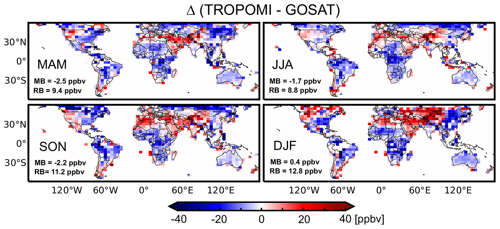
Figure 3Seasonally averaged differences (Δ) of between TROPOMI and GOSAT retrievals for May 2018–April 2019 on a 4∘ × 5∘ grid. The retrievals have been corrected for differences in averaging kernels and prior vertical profiles as described in the text. MB is the global mean bias of TROPOMI relative to GOSAT, and RB is the regional bias as defined by the standard deviation of Δ on the 4∘ × 5∘ grid.
We apply the same method for a more extensive analysis of regional differences between TROPOMI and GOSAT. Figure 3 shows the global distributions of the seasonal mean differences Δ between the two instruments, again correcting for differences in prior estimates and averaging kernels. The seasonal global mean biases for TROPOMI relative to GOSAT are consistent with the comparison to TCCON, but the regional biases are larger (8.8–12.8 ppbv), and some regions show differences of magnitude comparable to the regional enhancements of Fig. 1. The regional biases tend to be consistent across seasons, except for positive biases north of 40∘ N in DJF that could be associated with snow cover. These biases may affect TROPOMI's constraints on the seasonal variations in methane sources. We find particularly large differences between TROPOMI and GOSAT where the SWIR surface albedo is smaller than 0.1 as in Brazil, central Africa, and subarctic regions (see Fig. S1 in the Supplement). We may therefore expect large differences between TROPOMI and GOSAT inversions for these regions.
We assemble the 2019 TROPOMI and GOSAT observations of into an observation vector y, and we use the observations to optimize a state vector x consisting of methane sources and sinks. We use the GEOS-Chem global CTM version 12.5.0 (https://doi.org/10.5281/zenodo.3403111) at 2∘ × 2.5∘ grid resolution with 47 vertical layers as the forward model in the inversion. The model is essentially linear except for a small nonlinearity from the optimization of OH concentrations (Maasakkers et al., 2019). Prior estimates xa for methane sources are compiled from bottom-up inventories. We solve the Bayesian problem analytically to obtain both the posterior solution and its error covariance matrix . We conduct inversions using TROPOMI and GOSAT observations separately and together (joint inversion), and we also conduct additional inversions to examine the sensitivity of results to different parameters.
3.1 GEOS-Chem simulations and prior estimates
GEOS-Chem is driven by Modern-Era Retrospective analysis for Research and Applications, Version 2 (MERRA-2) meteorological fields from the NASA Global Modeling and Assimilation Office (GMAO). The original methane simulation is described by Wecht et al. (2014). Previous GEOS-Chem-based inversions at 4∘ × 5∘ horizontal resolution had excessive stratospheric methane poleward of 60∘ in winter–spring due to the inability to reproduce the polar vortex dynamical barrier, and this needed to be corrected in the inversion (Turner et al., 2015; Y. Zhang et al., 2021). The polar vortex dynamics are much better captured at 2∘ × 2.5∘ resolution (Stanevich et al., 2021; Y. Zhang et al., 2021), and we do not use satellite data poleward of 60∘ in our inversion anyway. There is therefore no need for stratospheric bias correction.
Table 1Global methane budget for 2019.
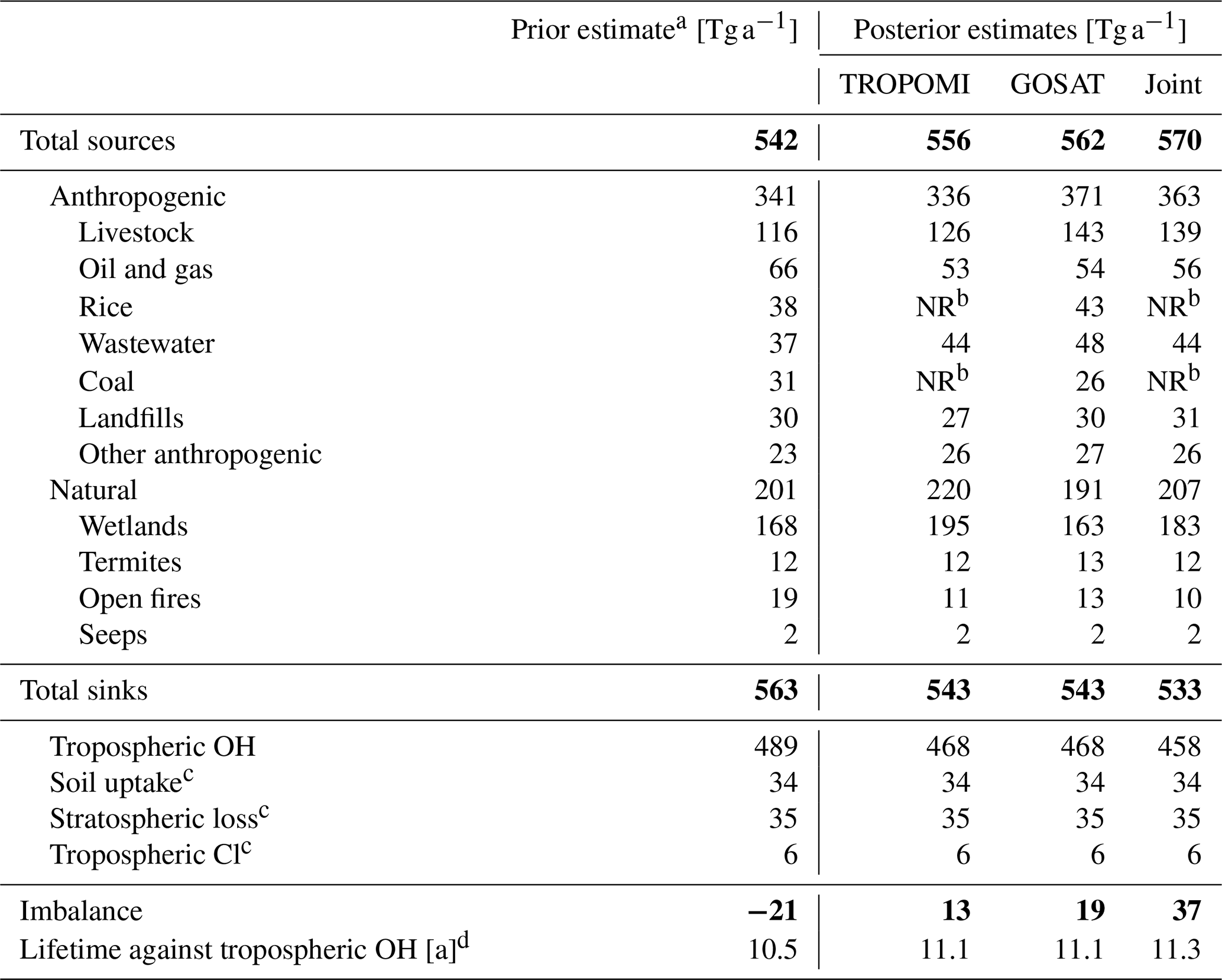
a Prior anthropogenic source estimates are from EDGAR v4.3.2 (Janssens-Maenhout et al., 2019) in 2012, superseded by oil, gas, and coal emissions from GFEI (Scarpelli et al., 2020) for 2016 and gridded EPA inventory data for the US (Maasakkers et al., 2016). Prior wetland emissions in 2019 are from WetCHARTs (Bloom et al., 2017). Open fire emissions are from the Global Fire Emissions Database version 4 (GFED4) in 2019 (van der Werf et al., 2017). Termite emissions are from Fung et al. (1991). Geological seepages are from Etiope et al. (2019) scaled to the global magnitude from Hmiel et al. (2020). b Not reported because of the potential for bias in the sectoral attribution of TROPOMI inversion results for China, which is a major global source of emissions from rice and coal. See text for details. c These minor sinks are not optimized by the inversion. d Lifetime of total atmospheric methane against oxidation by tropospheric OH.
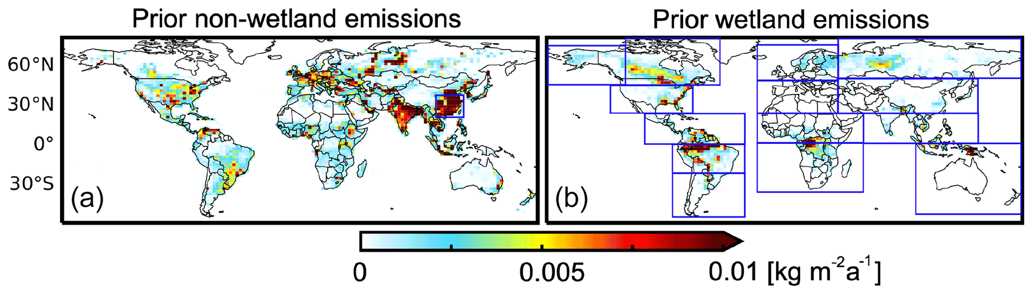
Figure 4Spatial distribution of prior methane emissions in 2019. The blue box over China in panel (a) indicates the region used for seasonality analysis in Fig. 8. The blue boxes in panel (b) indicate the 14 subcontinental regions of Y. Zhang et al. (2021) for which monthly wetland emissions are aggregated.
Table 1 summarizes the prior estimates of the sources and sinks of methane, and Fig. 4 shows the spatial distribution of the sources. The emissions from oil, gas, and coal exploitation are from the 2016 Global Fuel Exploitation Inventory (GFEI) version 1.0 (Scarpelli et al., 2020), which spatially allocates national emissions reported to the United Nations Framework Convention on Climate Change (UNFCCC). Other anthropogenic sources (livestock, landfills, wastewater, rice, etc.) are from the EDGAR v4.3.2 inventory in 2012 as global default (Janssens-Maenhout et al., 2019) and the gridded version of the US Environmental Protection Agency (EPA) greenhouse gas inventory in 2012 for the continental US (Maasakkers et al., 2016). Seasonalities of rice and manure emissions are based on B. Zhang et al. (2016) and Maasakkers et al. (2016), respectively.
We use monthly wetland methane emissions in 2019 from the 18-member ensemble mean of the WetCHARTs version 1.3.1 inventory (Bloom et al., 2017), which has good performance in reproducing the observed wetland methane seasonal cycle for most regions (Parker et al., 2020b). Other natural sources include open fire emissions in 2019 from the Global Fire Emissions Database version 4 (GFED4) (van der Werf et al., 2017), termite emissions from Fung et al. (1991), and geological seepage from Etiope et al. (2019) scaled to the global magnitude of 2 Tg a−1 from Hmiel et al. (2020). The total methane sources in the prior estimate add up to 542 Tg a−1, which is smaller than the bottom-up inventory estimate of 594–881 Tg a−1 from the Global Methane Budget 2020 (Saunois et al., 2020). The difference is mainly caused by the higher estimates of emissions from freshwater (117–212 Tg a−1), seeps (18–65 Tg a−1), oil and gas (72–97 Tg a−1), and coal (29–61 Tg a−1) in Saunois et al. (2020). The freshwater source in our prior estimate is included in the wetland sector as represented by WetCHARTs (Bloom et al., 2017).
The main sink of methane is oxidation by the hydroxyl radical (OH) in the troposphere (Ehhalt and Heidt, 1973), with a corresponding lifetime of 11.2 ± 1.3 years as constrained by the methyl chloroform proxy (Prather et al., 2012). Our prior estimate for the loss of methane from reaction with tropospheric OH is calculated using archived 3-D climatological monthly fields of OH concentrations from a GEOS-Chem full-chemistry simulation (Wecht et al., 2014), yielding a methane lifetime of 10.5 years due to oxidation by tropospheric OH. Additional minor losses include oxidation by tropospheric Cl atoms computed using archived Cl concentration fields from Wang et al. (2019), stratospheric oxidation computed with archived 2-D monthly loss frequencies from the NASA Global Modeling Initiative model (Murray et al., 2012), and soil uptake of methane specified following Murguia-Flores et al. (2018).
3.2 Analytical inversion
We apply Bayesian inference to optimize a state vector consisting of (1) annual mean non-wetland methane emissions for land-containing 2∘ × 2.5∘ grid cells (4020 state vector elements), (2) monthly wetland methane emissions for the 14 subcontinental regions of Fig. 4 (168 elements), and (3) annual hemispheric tropospheric OH concentrations (2 elements). Trade-off is needed between spatial and temporal resolution in the state vector to avoid smoothing error in the inversion (Wecht et al., 2014) and for computational tractability. For non-wetland emissions we use high spatial resolution but only optimize the annual mean values because seasonality is relatively small and predictable. For wetland emissions, we cannot assume that the prior seasonality is correct (Maasakkers et al., 2019) and instead optimize monthly emissions at coarse spatial resolution. This setup is the same as in Lu et al. (2021) and Y. Zhang et al. (2021) except for the higher horizontal resolution applied to non-wetland emissions. Together we have 4190 state vector elements, which require a total of 4190 perturbed GEOS-Chem simulations and a base simulation to construct the full Jacobian matrix. This is readily done on a high-performance computing platform as an embarrassingly parallel workload. Initial conditions on 1 January 2019 are obtained from a standard GEOS-Chem simulation using the prior emission estimates and a 10 year spin-up and are scaled by a globally uniform factor of 0.97 in order to match the global mean column mixing ratio retrieved from TROPOMI between 1 and 10 January 2019. This initialization efficiently reduces the normalized mean square error (NMSE) between GEOS-Chem and TROPOMI observations on 1 January 2019 from 0.37 to 0.02 and is used for both TROPOMI and GOSAT inversions.
The posterior estimate as defined by Bayesian inference assuming Gaussian error statistics is obtained by minimizing the scalar cost function J(x):
where K is the Jacobian matrix describing the sensitivity of the observations to the state vector as simulated by GEOS-Chem, Sa is the prior error covariance matrix, So is the observational error covariance matrix assumed to be diagonal, and γ is a regularization parameter that accounts for the effect of unresolved correlation in the observational error.
Sa is constructed by assuming 50 % prior error standard deviation for all non-wetland emissions on the 2∘ × 2.5∘ grid and 10 % prior error standard deviation for hemispheric annual mean OH concentrations, with no error correlations. Prior error variances and covariances for monthly wetland emissions in the 14 subcontinental regions are calculated using the WetCHARTs model ensemble (Bloom et al., 2017) following Y. Zhang et al. (2021).
Observational error variances (diagonal elements of So) are calculated using the residual error method (Heald et al., 2004) as the variance of the residual difference between observations and the GEOS-Chem prior simulation on the 2∘ × 2.5∘ grid after subtracting the mean difference. This method sums up errors from instrument retrieval, representation, and GEOS-Chem transport. We find a global annual mean error of 13 ppbv for TROPOMI and 14 ppbv for GOSAT. For cases where the calculated error is smaller than the instrument precision reported in the satellite retrieval, we use the latter instead (annual means of 9 ppbv for GOSAT and 2 ppbv for TROPOMI).
So is specified as diagonal but there is in fact some observational error covariance if only from the GEOS-Chem transport. For TROPOMI in particular, there may be many individual observations in a single GEOS-Chem grid cell for a given day, and the corresponding GEOS-Chem transport errors would be perfectly correlated. Although one could average all TROPOMI observations within a 2∘ × 2.5∘ grid cell before ingesting them in the inversion, this would lose the averaging kernel specificity for each observation. We therefore use a regularization parameter γ (Hansen et al., 1999; Y. Zhang et al., 2018, 2020; Maasakkers et al., 2019; Lu et al., 2021) to account for the off-diagonal structure missing in So. Based on the corner of the L-curve (Hansen et al., 1999) and the expected chi-square distribution of the cost function (Lu et al., 2021) (see Fig. S2 in the Supplement), we choose γ=0.002 for TROPOMI observations and γ=0.5 for GOSAT observations. The regularization parameter of 0.5 for GOSAT is larger than the values of 0.05–0.1 in Maasakkers et al. (2019), Y. Zhang et al. (2021), and Lu et al. (2021), because they used 4∘ × 5∘ resolution and several years of observations. The smaller value of γ for TROPOMI is due to its large number of collocated observations on the 2∘ × 2.5∘ model grid. Shen et al., (2021) conducted a regional inversion of TROPOMI data using GEOS-Chem at 0.25∘ × 0.3125∘ resolution and found that γ=0.25 provided the best fit to the L-curve, reflecting the much smaller number of collocated observations on the 0.25∘ × 0.3125∘ grid.
We further balance the prior terms in the cost function by weighing the wetland emission term by the number of elements in the state vector (4020/14). This step ensures that changes in non-wetland and wetland emissions are equally expensive from a cost-function perspective (Maasakkers et al., 2019). Similarly scaling the hemispheric OH terms in the cost function by the number of elements in the state vector (4020/2) would lead to excessively small posterior adjustments. We therefore choose weighting factors of the OH terms (400 for TROPOMI, 450 for GOSAT) that lead to a standard deviation of 5 % in the posterior OH adjustments.
There is some arbitrariness in the selection of regularization parameters γ and prior weighting factors in the inversion. In addition to the base inversion as described above, we examined the sensitivity to the choice of γ with sensitivity inversions using (1) γ=0.02 and (2) γ=0.5 for TROPOMI and (1) γ=0.02 and (2) γ=0.002 for GOSAT. We further examined the sensitivity to the choice of weighting factors with sensitivity inversions using (3) no weighting factors, (4) a weighting factor of 1 for wetland terms, and (5) a weighting factor of 2010 for the OH terms (i.e., the ratio of the number of state vector elements for non-wetland and OH terms). In this manner we performed six inversions using TROPOMI observations only (base inversion plus five sensitivity inversions), six inversions using GOSAT observations only, and 6 × 6 = 36 inversions using the joint TROPOMI and GOSAT observations.
The best posterior estimate obtained by minimization of the cost function J(x) is given by (Rodgers, 2000)
with posterior error covariance matrix :
The averaging kernel matrix A defines the sensitivity of the solution to the true state:
where I is the identity matrix. The trace of A represents the number of independent pieces of information on the state vector that is gained from the observations and is called the degrees of freedom for signal (DOFS) (Rodgers, 2000). Note that A here is different from the retrieval averaging kernel vectors in Sect. 2, which described the sensitivity of methane satellite retrievals to the vertical distribution of methane.
The posterior solution can also be presented in reduced dimensionality. For instance, posterior emissions on the 2∘ × 2.5∘ grid can be aggregated to national or global emissions from individual source sectors. This aggregation can be expressed with a summation matrix W to represent the linear transformation from the full state vector to the reduced state vector. The posterior estimate of the reduced state vector () is computed as
and its posterior error covariance and averaging kernel matrices are given by
where is the Moore–Penrose inverse (Calisesi et al., 2005).
Our discussion focuses principally on results from the base inversions of the TROPOMI-only, GOSAT-only, and joint TROPOMI+GOSAT observations and uses ranges from the inversion ensemble as a more conservative estimate of posterior errors than the posterior error covariance matrix . In this analysis we exclude ensemble members with unreasonable emission adjustments (e.g., negative emissions aggregated at regional scales) and OH adjustments larger than 40 % (see Tables S1 and S2 in the Supplement).

Figure 5Corrections to prior estimates of 2019 non-wetland methane emissions on the 2∘ × 2.5∘ grid (posterior prior ratios) and corresponding averaging kernel sensitivities. Results are shown for the TROPOMI, GOSAT, and joint TROPOMI + GOSAT inversions. Less than 3 % of grid cells have negative posterior prior ratios, which is allowed by the statistics but is likely unphysical. The averaging kernel sensitivities are the diagonal elements of the averaging kernel matrix for the inversion and measure the ability of the observations to constrain the emissions (1 = fully; 0 = not at all). The sum of averaging kernel sensitivities (trace of the averaging kernel matrix) defines the degrees of freedom for signal (DOFS) for the inversion, shown in the inset. DOFS including contributions from wetland emissions and OH concentrations are 155 for TROPOMI and 238 for GOSAT.
4.1 Information content from the inversions
Figure 5 shows the corrections to the prior estimates of non-wetland emissions (posterior prior ratios) on the 2∘ × 2.5∘ grid for the TROPOMI, GOSAT, and joint TROPOMI + GOSAT inversions. These corrections will be discussed in Sect. 4.3. Also shown are the averaging kernel sensitivities of the inversions, defined as the diagonal elements of the averaging kernel matrices and representing the ability of the observations to determine the posterior solution independently of the prior estimate (1 = fully; 0 = not at all). The averaging kernel sensitivities are highest over major anthropogenic source regions where the methane emissions are the largest.
The TROPOMI inversion has 155 DOFS, meaning that it contains 155 independent pieces of information on the distribution of methane emissions and OH concentrations. The GOSAT inversion has 238 DOFS, more than TROPOMI despite having much fewer observations. This reflects the large error correlation between individual TROPOMI observations on the 2∘ × 2.5∘ grid of the inversion, as expressed by the difference between the regularization parameters for GOSAT observations (γ=0.5) and TROPOMI observations (γ=0.002). GOSAT with precise individual observations spaced by 250 km is particularly well adapted to an inversion on a 2∘ × 2.5∘ grid. TROPOMI would be far more valuable in a regional inversion at higher spatial resolution (Shen et al., 2021), although the regional biases discussed in Sect. 2 would still be a concern.
Y. Zhang et al. (2021) previously reported an inversion of 2010–2018 GOSAT data using GEOS-Chem at 4∘ × 5∘ resolution. That inversion achieved 179 DOFS, compared to 238 DOFS in our inversion for just 1 year of GOSAT data at 2∘ × 2.5∘ resolution. The higher DOFS in our case reflects the higher dimension of our emission state vector (2∘ × 2.5∘ versus 4∘ × 5∘ grid cells), combined with higher weight per observation (γ=0.5 versus 0.05) because of lower error correlation on the 2∘ × 2.5∘ scale. As pointed out above, the GOSAT data are particularly well suited to a 2∘ × 2.5∘ resolution for the inversion. The finer 2∘ × 2.5∘ resolution allows for improved sectoral and national attribution of inversion results as will be done in Sect. 4.3.
In the joint inversion, TROPOMI observations add additional DOFS to the GOSAT posterior at 0∘ –30∘ N (mainly over India and the Middle East, Figs. 5 and S3 in the Supplement), where TROPOMI has more observations than in the rest of the world (Fig. 1). TROPOMI has lower averaging kernel sensitivities at 30–60∘ N and 0–60∘ S, and the information content over these two regions mostly comes from GOSAT. This could reflect the limitation of using a single global regularization parameter γ for the TROPOMI observations, because the observations should have more weight (larger γ) when they are less dense. Improving this aspect of the inversion is a target for future work.
The 155 DOFS for TROPOMI are partitioned as 151 for non-wetland emissions, 3 for wetlands, and 1 for OH. The 238 DOFS for GOSAT are partitioned as 232 for non-wetland emissions, 5 for wetlands, and 1 for OH. The wetland emissions are largely unchanged in both inversions because of error weighting in the cost function that penalizes departure from the prior estimate. Without this error weighting, the TROPOMI inversion would yield unrealistic wetland emissions and seasonalities (case 3 in Table S1). The problem may reflect systematic biases in the TROPOMI retrieval due to the low SWIR surface albedo over wetland surfaces (e.g., Brazil and central Africa (see Fig. S4 in the Supplement) and boreal wetlands in Canada and Russia), combined with seasonal imbalance in observations (cloudiness for tropical wetlands, sun angle and snow for boreal wetlands) and seasonal biases at high northern latitudes (Fig. 3). The GOSAT-only inversion without error weighting for wetlands shows no such problems, but we still apply error weighting in that base inversion for comparison to TROPOMI. Improvement in TROPOMI retrievals over wetlands is clearly needed. In the meantime, our further discussion of results in Sect. 4.3 will focus on the non-wetland emissions.
The posterior prior ratio of global OH concentrations is 0.96 for both the TROPOMI and GOSAT inversions and 0.91 for the joint inversion. Methane lifetimes against oxidation by tropospheric OH range from 10.7 to 11.0 years in the ensemble of TROPOMI inversions excluding case 3 (Table S1) and from 10.7 to 11.1 years in the GOSAT inversions (Table S2). These corrections improve agreement with the observationally constrained methane lifetime of 11.2 ± 1.3 years (Prather et al., 2012). The north–south interhemispheric OH ratio () is 1.03 in the prior estimate, 0.93 in the TROPOMI inversion, 1.15 in the GOSAT inversion, and 1.03 in the joint inversion, suggesting that the observations do not usefully constrain this ratio. Patra et al. (2014) estimated a ratio of 0.97 ± 0.12 from methyl chloroform observations.

Figure 6Comparison of GEOS-Chem to TROPOMI and GOSAT observations. Panels show annual mean differences for 2019 between the GEOS-Chem simulation and observations, with mean bias ± standard deviation given in the inset. The top panels show GEOS-Chem with prior emission and OH estimates. The middle panels show GEOS-Chem with posterior estimates from the TROPOMI inversion. The bottom panels show GEOS-Chem with posterior estimates from the GOSAT inversion.
4.2 Cross-fit to TROPOMI and GOSAT observations
Figure 6 shows the ability of the inversions to improve the fit between GEOS-Chem and the 2019 satellite observations when using posterior versus prior emissions and OH concentrations. This includes cross-evaluation of the TROPOMI inversion with independent GOSAT observations and vice versa. The simulation using prior emissions started on 1 January 2019 in an unbiased state compared to TROPOMI and a −1.7 ppbv global bias relative to GOSAT (Sect. 2). It underestimates 2019 GOSAT observations everywhere by an average of 14.6 ppbv (Fig. 6), implying the need to increase methane sources and/or decrease OH concentrations. It also underestimates TROPOMI over most of the world but overestimates in some regions (notably the subarctic) that may reflect TROPOMI retrieval biases as discussed in Sect. 2.
Both TROPOMI and GOSAT inversions reduce the negative differences between simulations and observations. The improvement can be measured by the value of the cost function J(x) in Eq. (3), which decreases by 35 % for the TROPOMI inversion and 54 % for the GOSAT inversion. GOSAT observations are still underestimated by an average of 5.3 ppbv in the GOSAT inversion because the information from the observations is not sufficient to fully correct the bias in the prior estimate. Cross-evaluation of the posterior simulation with the independent data set (TROPOMI or GOSAT) also shows improvement. The fit to the GOSAT data is improved everywhere even with the TROPOMI inversion. TROPOMI shows problematic regions where the inversion overcorrects the prior bias. This will be discussed further in Sect. 4.3.
4.3 Implications for methane emissions
4.3.1 Global distribution
Our posterior prior ratios for the 2019 GOSAT inversion in Fig. 5 show large upward adjustments of non-wetland emissions in the south-central US, Venezuela, and the Middle East, consistent in magnitude with the previous inversion of 2010–2018 GOSAT data by Y. Zhang et al. (2021), who used the same prior estimate. These two inversions also have consistent magnitude of downward adjustments in the western US, Europe, Russia, and North China Plain. We find larger upward adjustments than Y. Zhang et al. (2021) in India, East Africa, and Brazil, which they identified as regions with rapidly increasing emissions over the 2010–2018 period.
Figure 5 shows agreement between GOSAT and TROPOMI in the adjustments of methane emissions in several major source regions including western Russia, the North China Plain, the south-central US, East Africa, and Venezuela. A few regions have adjustments of different signs, notably Brazil and parts of central Africa where the TROPOMI retrievals are likely biased (Figs. 3 and S4).
We conducted a global sectoral breakdown of the posterior non-wetland emission fluxes on the 2∘ × 2.5∘ grid by using Eq. (7), where we assume the partitioning between sectors in a given grid cell to be correct in the prior inventory and the posterior prior ratio to apply equally to all sectors in the grid cell. This assumption is due to the lack of additional information (e.g., isotopic fractionation; Ghosh et al., 2015; G. Zhang et al., 2016; Zazzeri et al., 2017) to separate different sources. Our restricted adjustment of wetland emissions due to increased weight in the cost function means that errors in wetland emissions could be projected to non-wetland sectors. For example, for the TROPOMI-only inversion, global posterior non-wetland emissions are 361 Tg a−1 in the base inversion and 389 Tg a−1 in the sensitivity inversion without increased weight for wetland emissions (Table S1). For the GOSAT inversion the effect is much less, 399 versus 404 Tg a−1 (Table S2).
Table 1 compiles our sectoral attributions of inversion results. Of particular interest is the oil–gas sector, for which the global prior estimate (66 Tg a−1) is based on 2016 UNFCCC national inventory reports. We find global decreases in the joint TROPOMI + GOSAT inversion to 56 Tg a−1, largely driven by decreases in Russia. This is consistent with the correction in Russian oil–gas emissions reported to the UNFCCC, from 27 Tg a−1 in the communication used by the GFEI to 16 Tg a−1 in the latest communication (UNFCCC, 2020). Livestock emissions (the single largest anthropogenic methane source) are adjusted upward by the joint inversion from 116 Tg a−1 in the EDGAR v4.3.2 prior estimate to 139 Tg a−1.
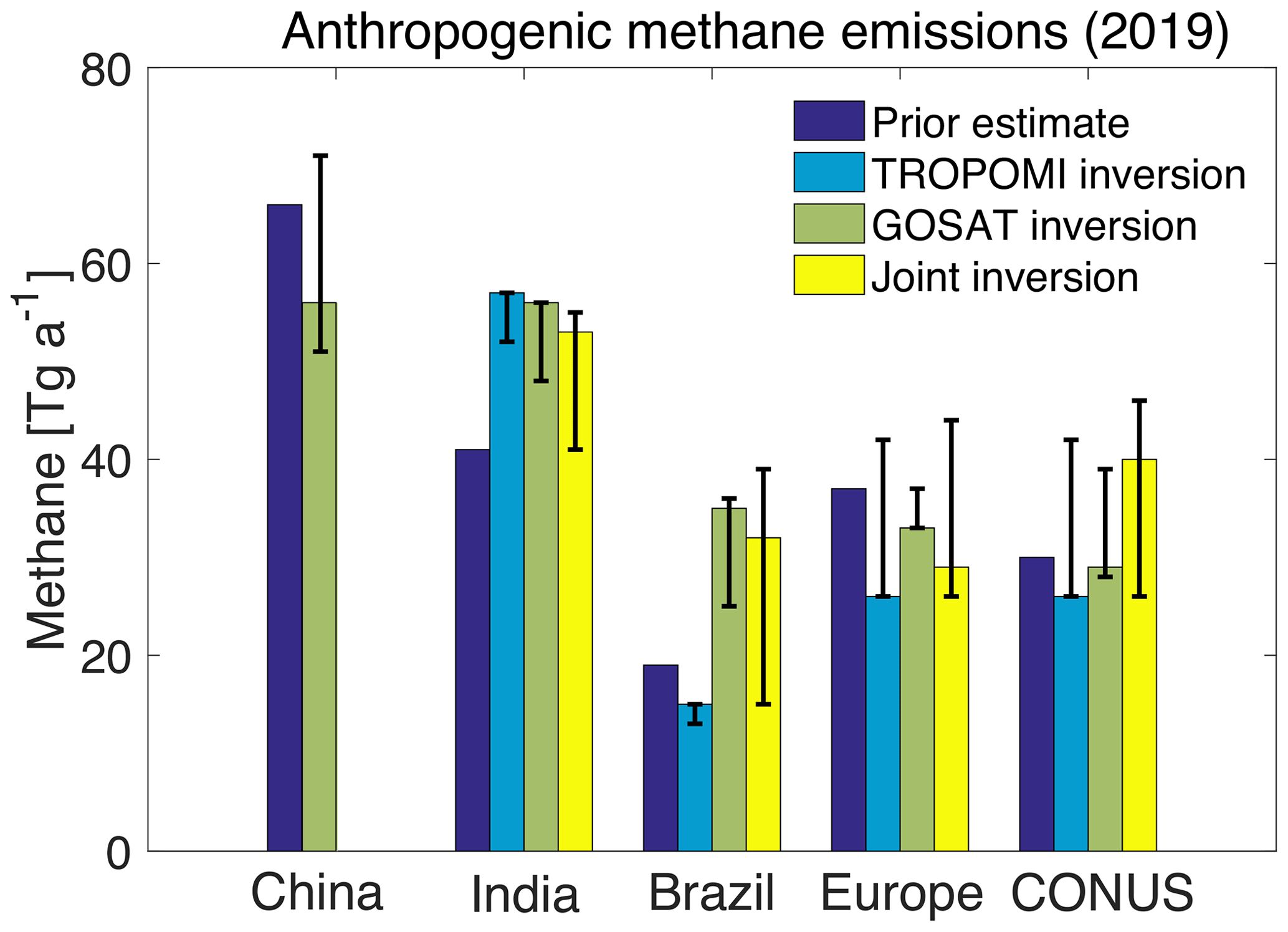
Figure 7Annual anthropogenic methane emissions in 2019 for five major source regions, accounting for 56 % of global anthropogenic emissions in the inversion of GOSAT data. The vertical bars represent the range of posterior emissions from the ensemble of inversions. Europe is defined as west of 37∘ E. The CONUS is the contiguous United States. TROPOMI and joint inversion results are not shown for China because of concern over biases resulting from seasonal cloudiness and prior errors in the spatial distribution of coal emissions (see text).
4.3.2 Major source regions
Figure 7 shows emissions in the top five anthropogenic methane source regions including China, India, Brazil, Europe, and the contiguous US (CONUS). These regions account for 56 % of global posterior anthropogenic emissions in the GOSAT inversion.

Figure 8Seasonality of methane emissions from rice cultivation and satellite observation frequency over southeast China (20–37∘ N, 103–123∘ E, shown in Fig. 4) in 2019. The number of TROPOMI observations increases after August 2019 due to change in pixel size from 2 km × 2.5 km to 5.5 km × 7 km. Seasonality of rice emissions is from B. Zhang et al. (2016). Note the difference in scale for the number of observations by TROPOMI and GOSAT.
In China, both GOSAT and TROPOMI inversions adjust non-wetland methane emissions downward in the North China Plain (Fig. 5). This has been a long-standing result of inversions of satellite data using EDGAR v4.1 and v4.2 as the prior estimate (Monteil et al., 2013; Thompson et al., 2015; Alexe et al., 2015; Turner et al., 2015) and has been attributed to an overestimate of emissions from the coal sector which dominates total EDGAR emissions in the region. More recent inversions using the UNFCCC-based GFEI as the prior estimate have found the same result (Lu et al., 2021; Y. Zhang et al., 2021), but GFEI takes its spatial allocation of coal emissions from EDGAR v4.3.2. A more detailed bottom-up analysis by Sheng et al. (2019) finds most of the Chinese coal emissions to be in south China, in contrast to EDGAR which places them in the North China Plain. Our TROPOMI inversion over southeast China shows spatially inconsistent results with the GOSAT inversion (Fig. 5) and overcorrects the fit to observations (Fig. 6), which may be due to aliasing between coal and rice emissions. Rice cultivation is the dominant source of methane in southeast China in our prior estimate, but the emissions have large seasonality and peak in summer when cloudiness is pervasive and TROPOMI observations are few, as shown in Fig. 8. GOSAT is less affected by cloudiness (Fig. 8), on account of its use of the CO2 proxy retrieval method. We therefore exclude posterior estimates from TROPOMI and the joint inversions from Fig. 7. Because China accounts for a large fraction of global rice (Chen et al., 2013) and coal emissions (Cheng et al., 2011; Miller et al., 2019), we also exclude these entries from Table 1. At national scale, the GOSAT inversion adjusts anthropogenic methane emissions downward from 67 to 56 Tg a−1 in China, very close to the value of 55 Tg a−1 in the latest report by China to the UNFCCC in 2014.
All three inversions adjust methane emissions upwards in India. The results from the base inversion are at the higher end of the range from the inversion ensemble, but the 41–57 Tg a−1 range of national emissions spanned by the ensemble is still much higher than previous inversions of GOSAT and in situ data including 33 Tg a−1 for 2010–2018 by Y. Zhang et al. (2021) and 22 Tg a−1 for 2010–2015 by Ganesan et al. (2017). This may reflect the rapid increase in Indian emissions over the 2010–2018 period previously identified by Y. Zhang et al. (2021) and attributed principally to livestock.
In Brazil, the large upward adjustments from 19 Tg a−1 (prior) to 35 Tg a−1 (GOSAT) and 32 Tg a−1 (joint) in the posterior estimates are consistent with previous top-down estimates (Maasakkers et al., 2019; Y. Zhang et al., 2021). TROPOMI shows adjustments in the opposite direction, likely reflecting observational bias associated with low SWIR surface albedo (Fig. 3) and limited number of observations. The joint inversion is dominated by results from GOSAT on account of the much higher averaging kernel sensitivities for the inversion (Fig. 5).
All inversions adjust emissions downwards in Europe (prior: 37 Tg a−1; TROPOMI: 26 Tg a−1; GOSAT: 33 Tg a−1; joint: 29 Tg a−1), consistent with the previous downward adjustments in the 2010–2018 mean in the GOSAT inversion and the small negative trend in methane emissions (Y. Zhang et al., 2021). The largest reductions of emissions in Europe are from coal and oil–gas emissions.
In the CONUS, the large upward adjustment in the south-central region reflects the well-known underestimate of oil–gas emissions by the US EPA inventory in that region (Kort et al., 2014; Smith et al., 2017; Peischl et al., 2018; Alvarez et al., 2018; Maasakkers et al., 2021; Gorchov Negron et al., 2020; Y. Zhang et al., 2021; Lyon et al., 2021). The posterior estimates from both TROPOMI and GOSAT adjust national methane emissions slightly downwards from 30 to 26 Tg a−1 (TROPOMI) and 29 Tg a−1 (GOSAT) over the CONUS, close to the posterior estimates of 31 Tg a−1 from the 0.5∘ × 0.625∘ inversion over 2010–2015 (Maasakkers et al., 2021). The joint inversion adjusts emissions upwards to 40 Tg a−1 due to the larger averaging kernel sensitivity over the south-central US, where emissions have large upward adjustments.
We used 1 year (2019) of atmospheric methane column observations from the new TROPOMI satellite instrument in a global inverse analysis of methane sources at 2∘ × 2.5∘ resolution, and we compared results to the same analysis using the more mature but sparser GOSAT instrument as well as the combination of the two instruments. By analytical solution to the inverse problem, we were able to quantitatively compare the information content from the two satellite data sets. This includes averaging kernel sensitivities and degrees of freedom for signal (DOFS) that quantify the number of independent pieces of information on the distribution of methane emissions.
We began by validating the global observations from TROPOMI and GOSAT by common reference to the ground-based TCCON methane column measurements, using the GEOS-Chem CTM to correct for the effects of different prior estimates and averaging kernels in the retrievals from each instrument. Results show that TROPOMI and GOSAT are globally biased by −2.7 and −1.0 ppbv, respectively. Their regional biases relative to TCCON are 7 and 3 ppbv, respectively, sufficiently small for inverse analyses of methane emissions on regional to global scales. Intercomparison between TROPOMI and GOSAT shows larger regional differences exceeding 20 ppbv, generally in places where the SWIR surface albedo is low and TROPOMI retrievals would be subject to biases (Lorente et al., 2021). GOSAT is less sensitive to albedo-driven biases because of its CO2 proxy retrieval method, compared to the full-physics retrieval in TROPOMI.
We find that the GOSAT inversion has a global DOFS of 232 for non-wetland methane emissions on the 2∘ × 2.5∘ grid, larger than the TROPOMI inversion (DOFS of 151) despite the TROPOMI data being much denser. This is because individual TROPOMI observations have large error correlations on the 2∘ × 2.5∘ grid of the inversion, whereas the GOSAT observations with their 250 km separation are ideally suited for our 2∘ × 2.5∘ inversion scale. Finer-scale inversions, as done for regional studies, would be far more effective at exploiting the information from TROPOMI. A better representation of error correlation, accounting for the relative sparsity of TROPOMI data in cloudy regions, would also increase the value of TROPOMI data in global inversions. Combining the TROPOMI and GOSAT data in a joint inversion increases the DOFS to 244, with most of the added information from TROPOMI in the 0–30∘ N latitudinal band including India and the Middle East.
The TROPOMI and GOSAT inversions for 2019 show consistent upward adjustments of anthropogenic methane emissions over Venezuela (oil–gas) and the south-central US (oil–gas) and downward adjustments over Europe (oil–gas and coal), Russia (oil–gas), and the North China Plain (coal). These adjustments are relative to the official national inventory reports to the UNFCCC in 2016 and used as prior estimates in our inversion. The TROPOMI and GOSAT inversions also show consistent upward adjustments over East Africa where livestock emissions are large. Global livestock emissions increase from 116 Tg a−1 in the EDGAR v4.3.2 prior estimate to 139 Tg a−1 in the joint GOSAT+TROPOMI inversion. Some regions show large inconsistencies between TROPOMI and GOSAT inversions, and we find that these generally reflect TROPOMI regional biases in low-albedo regions. The strict cloudiness filter used in TROPOMI observations is also problematic in methane source regions such as wetlands and rice agriculture that have extensive and sometimes seasonal cloud cover.
Our results demonstrate the potential of applying TROPOMI observations to constrain methane emissions on a global scale through inverse analyses but also stress the need for caution. The methane retrieval from TROPOMI is still in an early stage, and the current operational product appears to have systematic biases in low-albedo regions. Future generations of the retrieval may address these data quality flaws (Lorente et al., 2021). Improved accounting of model transport error correlations is also needed to fully exploit the inversion of TROPOMI observations on a global scale. In the meantime, GOSAT provides a high-quality record of methane observations going back to 2010, and we have shown that 1 year of GOSAT observations can usefully inform emissions on a 2∘ × 2.5∘ grid. GOSAT will be increasingly useful in the future to attribute methane trends and to validate future generations of the TROPOMI retrieval.
The TROPOMI methane observations are downloaded from http://www.tropomi.eu/data-products/methane (last access: 8 August 2020). The GOSAT methane retrieval is available at https://catalogue.ceda.ac.uk/uuid/18ef8247f52a4cb6a14013f8235cc1eb (last access: 29 December 2020). The TCCON measurements are downloaded from https://data.caltech.edu/records/293 (last access: 6 September 2020).
The supplement related to this article is available online at: https://doi.org/10.5194/acp-21-14159-2021-supplement.
ZQ and DJJ designed the study. ZQ conducted the modeling and data analyses with contributions from LS, XL, YZ, HN, MPS, JDM, and JRW. TRS contributed to the GFEI emission inventory and its interpretation. AAB contributed to the WetCHARTs wetland emission inventory and its interpretation. RJP provided the GOSAT methane retrievals. ALD contributed to the TROPOMI methane retrievals. ZQ and DJJ wrote the paper with input from all authors.
The authors declare that they have no conflict of interest.
Publisher's note: Copernicus Publications remains neutral with regard to jurisdictional claims in published maps and institutional affiliations.
This work was funded by the NASA Carbon Monitoring System under NASA award number 80NSSC18K0178 to Harvard University. Robert J. Parker is funded via the UK National Centre for Earth Observation (NE/N018079/1). We thank the Japanese Aerospace Exploration Agency, National Institute for Environmental Studies, and the Ministry of Environment for the GOSAT data and their continuous support as part of the Joint Research Agreement. This research used the ALICE High Performance Computing Facility at the University of Leicester for the GOSAT retrievals. Part of this research was carried out at the Jet Propulsion Laboratory, California Institute of Technology, under a contract with the National Aeronautics and Space Administration. Yuzhong Zhang acknowledges funding from NSFC (project 42007198) and Westlake University.
This research has been supported by NASA (grant no. 80NSSC18K0178), NSFC (grant no. 42007198), and the UK National Centre for Earth Observation (grant no. NE/N018079/1).
This paper was edited by Eduardo Landulfo and reviewed by two anonymous referees.
Alexe, M., Bergamaschi, P., Segers, A., Detmers, R., Butz, A., Hasekamp, O., Guerlet, S., Parker, R., Boesch, H., Frankenberg, C., Scheepmaker, R. A., Dlugokencky, E., Sweeney, C., Wofsy, S. C., and Kort, E. A.: Inverse modelling of CH4 emissions for 2010–2011 using different satellite retrieval products from GOSAT and SCIAMACHY, Atmos. Chem. Phys., 15, 113–133, https://doi.org/10.5194/acp-15-113-2015, 2015.
Alvarez, R. A., Zavala-Araiza, D., Lyon, D. R., Allen, D. T., Barkley, Z. R., Brandt, A. R., Davis, K. J., Herndon, S. C., Jacob, D. J., Karion, A., Kort, E. A., Lamb, B. K., Lauvaux, T., Maasakkers, J. D., Marchese, A. J., Omara, M., Pacala, S. W., Peischl, J., Robinson, A. L., Shepson, P. B., Sweeney, C., Townsend-Small, A., Wofsy, S. C., and Hamburg, S. P.: Assessment of methane emissions from the U. S. oil and gas supply chain, Science, 361, 186–188, https://doi.org/10.1126/science.aar7204, 2018.
Baray, S., Jacob, D. J., Massakkers, J. D., Sheng, J.-X., Sulprizio, M. P., Jones, D. B. A., Bloom, A. A., and McLaren, R.: Estimating 2010–2015 Anthropogenic and Natural Methane Emissions in Canada using ECCC Surface and GOSAT Satellite Observations, Atmos. Chem. Phys. Discuss. [preprint], https://doi.org/10.5194/acp-2020-1195, in review, 2021.
Bloom, A. A., Bowman, K. W., Lee, M., Turner, A. J., Schroeder, R., Worden, J. R., Weidner, R., McDonald, K. C., and Jacob, D. J.: A global wetland methane emissions and uncertainty dataset for atmospheric chemical transport models (WetCHARTs version 1.0), Geosci. Model Dev., 10, 2141–2156, https://doi.org/10.5194/gmd-10-2141-2017, 2017.
Brasseur, G. P. and Jacob, D. J.: Modeling of Atmospheric Chemistry, in: Modeling of Atmospheric Chemistry, Cambridge University Press, Cambridge, i-i, 2017.
Buchwitz, M., Reuter, M., Schneising, O., Boesch, H., Guerlet, S., Dils, B., Aben, I., Armante, R., Bergamaschi, P., Blumenstock, T., Bovensmann, H., Brunner, D., Buchmann, B., Burrows, J. P., Butz, A., Chédin, A., Chevallier, F., Crevoisier, C. D., Deutscher, N. M., Frankenberg, C., Hase, F., Hasekamp, O. P., Heymann, J., Kaminski, T., Laeng, A., Lichtenberg, G., De Mazière, M., Noël, S., Notholt, J., Orphal, J., Popp, C., Parker, R., Scholze, M., Sussmann, R., Stiller, G. P., Warneke, T., Zehner, C., Bril, A., Crisp, D., Griffith, D. W. T., Kuze, A., O'Dell, C., Oshchepkov, S., Sherlock, V., Suto, H., Wennberg, P., Wunch, D., Yokota, T., and Yoshida, Y.: The Greenhouse Gas Climate Change Initiative (GHG-CCI): Comparison and quality assessment of near-surface-sensitive satellite-derived CO2 and CH4 global data sets, Remote Sens. Environ., 162, 344–362, https://doi.org/10.1016/j.rse.2013.04.024, 2015.
Butz, A., Guerlet, S., Hasekamp, O., Schepers, D., Galli, A., Aben, I., Frankenberg, C., Hartmann, J.-M., Tran, H., Kuze, A., Keppel-Aleks, G., Toon, G., Wunch, D., Wennberg, P., Deutscher, N., Griffith, D., Macatangay, R., Messerschmidt, J., Notholt, J., and Warneke, T.: Toward accurate CO2 and CH4 observations from GOSAT, Geophys. Res. Lett., 38, L14812, https://doi.org/10.1029/2011gl047888, 2011.
Butz, A., Galli, A., Hasekamp, O., Landgraf, J., Tol, P., and Aben, I.: TROPOMI aboard Sentinel-5 Precursor: Prospective performance of CH4 retrievals for aerosol and cirrus loaded atmospheres, Remote Sens. Environ., 120, 267–276, https://doi.org/10.1016/j.rse.2011.05.030, 2012.
Calisesi, Y., Soebijanta, V. T., and van Oss, R.: Regridding of remote soundings: Formulation and application to ozone profile comparison, J. Geophys. Res.-Atmos., 110, D23306, https://doi.org/10.1029/2005JD006122, 2005.
Chen, H., Zhu, Q. A., Peng, C., Wu, N., Wang, Y., Fang, X., Jiang, H., Xiang, W., Chang, J., Deng, X., and Yu, G.: Methane emissions from rice paddies natural wetlands, lakes in China: synthesis new estimate, Glob. Change Biol., 19, 19–32, https://doi.org/10.1111/gcb.12034, 2013.
Chen, Y.-H. and Prinn, R. G.: Estimation of atmospheric methane emissions between 1996 and 2001 using a three-dimensional global chemical transport model, J. Geophys. Res.-Atmos., 111, D10307, https://doi.org/10.1029/2005JD006058, 2006.
Cheng, Y.-P., Wang, L., and Zhang, X.-L.: Environmental impact of coal mine methane emissions and responding strategies in China, Int. J. Greenh. Gas Con., 5, 157–166, https://doi.org/10.1016/j.ijggc.2010.07.007, 2011.
Connor, B. J., Boesch, H., Toon, G., Sen, B., Miller, C., and Crisp, D.: Orbiting Carbon Observatory: Inverse method and prospective error analysis, J. Geophys. Res.-Atmos., 113, D05305, https://doi.org/10.1029/2006jd008336, 2008.
Cressot, C., Chevallier, F., Bousquet, P., Crevoisier, C., Dlugokencky, E. J., Fortems-Cheiney, A., Frankenberg, C., Parker, R., Pison, I., Scheepmaker, R. A., Montzka, S. A., Krummel, P. B., Steele, L. P., and Langenfelds, R. L.: On the consistency between global and regional methane emissions inferred from SCIAMACHY, TANSO-FTS, IASI and surface measurements, Atmos. Chem. Phys., 14, 577–592, https://doi.org/10.5194/acp-14-577-2014, 2014.
Ehhalt, D. H., and Heidt, L. E.: The concentration of molecular H2 and CH4 in the stratosphere, Pure Appl. Geophys., 106, 1352–1360, https://doi.org/10.1007/BF00881090, 1973.
Etiope, G., Ciotoli, G., Schwietzke, S., and Schoell, M.: Gridded maps of geological methane emissions and their isotopic signature, Earth Syst. Sci. Data, 11, 1–22, https://doi.org/10.5194/essd-11-1-2019, 2019.
Fraser, A., Palmer, P. I., Feng, L., Boesch, H., Cogan, A., Parker, R., Dlugokencky, E. J., Fraser, P. J., Krummel, P. B., Langenfelds, R. L., O'Doherty, S., Prinn, R. G., Steele, L. P., van der Schoot, M., and Weiss, R. F.: Estimating regional methane surface fluxes: the relative importance of surface and GOSAT mole fraction measurements, Atmos. Chem. Phys., 13, 5697–5713, https://doi.org/10.5194/acp-13-5697-2013, 2013.
Fung, I., John, J., Lerner, J., Matthews, E., Prather, M., Steele, L. P., and Fraser, P. J.: Three-dimensional model synthesis of the global methane cycle, J. Geophys. Res.-Atmos., 96, 13033–13065, https://doi.org/10.1029/91JD01247, 1991.
Ganesan, A. L., Rigby, M., Lunt, M. F., Parker, R. J., Boesch, H., Goulding, N., Umezawa, T., Zahn, A., Chatterjee, A., Prinn, R. G., Tiwari, Y. K., van der Schoot, M., and Krummel, P. B.: Atmospheric observations show accurate reporting and little growth in India's methane emissions, Nat. Commun., 8, 836, https://doi.org/10.1038/s41467-017-00994-7, 2017.
Ghosh, A., Patra, P. K., Ishijima, K., Umezawa, T., Ito, A., Etheridge, D. M., Sugawara, S., Kawamura, K., Miller, J. B., Dlugokencky, E. J., Krummel, P. B., Fraser, P. J., Steele, L. P., Langenfelds, R. L., Trudinger, C. M., White, J. W. C., Vaughn, B., Saeki, T., Aoki, S., and Nakazawa, T.: Variations in global methane sources and sinks during 1910–2010, Atmos. Chem. Phys., 15, 2595–2612, https://doi.org/10.5194/acp-15-2595-2015, 2015.
Gorchov Negron, A. M., Kort, E. A., Conley, S. A., and Smith, M. L.: Airborne Assessment of Methane Emissions from Offshore Platforms in the U. S. Gulf of Mexico, Environ. Sci. Technol., 54, 5112–5120, https://doi.org/10.1021/acs.est.0c00179, 2020.
Hansen, P. C.: The L-curve and its use in the numerical treatment of inverse problems, IMM Tech. Rep. 15/1999, Kongens Lyngby, Denmark, 1999.
Hasekamp, O., Lorente, A., Hu, H., Butz, A., aan de Brugh, J., and Landgraf, J.: Algorithm Theoretical Baseline Document for Sentinel-5 Precursor Methane Retrieval, available at: https://sentinel.esa.int/documents/247904/2476257/Sentinel-5P-TROPOMI-ATBD-Methane-retrieval, last access: 14 March 2021.
Heald, C. L., Jacob, D. J., Jones, D. B. A., Palmer, P. I., Logan, J. A., Streets, D. G., Sachse, G. W., Gille, J. C., Hoffman, R. N., and Nehrkorn, T.: Comparative inverse analysis of satellite (MOPITT) and aircraft (TRACE-P) observations to estimate Asian sources of carbon monoxide, J. Geophys. Res.-Atmos., 109, D23306, https://doi.org/10.1029/2004JD005185, 2004.
Henne, S., Brunner, D., Oney, B., Leuenberger, M., Eugster, W., Bamberger, I., Meinhardt, F., Steinbacher, M., and Emmenegger, L.: Validation of the Swiss methane emission inventory by atmospheric observations and inverse modelling, Atmos. Chem. Phys., 16, 3683–3710, https://doi.org/10.5194/acp-16-3683-2016, 2016.
Hmiel, B., Petrenko, V. V., Dyonisius, M. N., Buizert, C., Smith, A. M., Place, P. F., Harth, C., Beaudette, R., Hua, Q., Yang, B., Vimont, I., Michel, S. E., Severinghaus, J. P., Etheridge, D., Bromley, T., Schmitt, J., Faïn, X., Weiss, R. F., and Dlugokencky, E.: Preindustrial 14CH4 indicates greater anthropogenic fossil CH4 emissions, Nature, 578, 409–412, https://doi.org/10.1038/s41586-020-1991-8, 2020.
Houweling, S., Krol, M., Bergamaschi, P., Frankenberg, C., Dlugokencky, E. J., Morino, I., Notholt, J., Sherlock, V., Wunch, D., Beck, V., Gerbig, C., Chen, H., Kort, E. A., Röckmann, T., and Aben, I.: A multi-year methane inversion using SCIAMACHY, accounting for systematic errors using TCCON measurements, Atmos. Chem. Phys., 14, 3991–4012, https://doi.org/10.5194/acp-14-3991-2014, 2014.
Hu, H., Hasekamp, O., Butz, A., Galli, A., Landgraf, J., Aan de Brugh, J., Borsdorff, T., Scheepmaker, R., and Aben, I.: The operational methane retrieval algorithm for TROPOMI, Atmos. Meas. Tech., 9, 5423–5440, https://doi.org/10.5194/amt-9-5423-2016, 2016.
Hu, H., Landgraf, J., Detmers, R., Borsdorff, T., Aan de Brugh, J., Aben, I., Butz, A., and Hasekamp, O.: Toward Global Mapping of Methane With TROPOMI: First Results and Intersatellite Comparison to GOSAT, Geophys. Res. Lett., 45, 3682–3689, https://doi.org/10.1002/2018gl077259, 2018.
Jacob, D. J., Turner, A. J., Maasakkers, J. D., Sheng, J., Sun, K., Liu, X., Chance, K., Aben, I., McKeever, J., and Frankenberg, C.: Satellite observations of atmospheric methane and their value for quantifying methane emissions, Atmos. Chem. Phys., 16, 14371–14396, https://doi.org/10.5194/acp-16-14371-2016, 2016.
Janssens-Maenhout, G., Crippa, M., Guizzardi, D., Muntean, M., Schaaf, E., Dentener, F., Bergamaschi, P., Pagliari, V., Olivier, J. G. J., Peters, J. A. H. W., van Aardenne, J. A., Monni, S., Doering, U., Petrescu, A. M. R., Solazzo, E., and Oreggioni, G. D.: EDGAR v4.3.2 Global Atlas of the three major greenhouse gas emissions for the period 1970–2012, Earth Syst. Sci. Data, 11, 959–1002, https://doi.org/10.5194/essd-11-959-2019, 2019.
Kort, E. A., Frankenberg, C., Costigan, K. R., Lindenmaier, R., Dubey, M. K., and Wunch, D.: Four corners: The largest US methane anomaly viewed from space, Geophys. Res. Lett., 41, 6898–6903, https://doi.org/10.1002/2014GL061503, 2014.
Kuze, A., Suto, H., Shiomi, K., Kawakami, S., Tanaka, M., Ueda, Y., Deguchi, A., Yoshida, J., Yamamoto, Y., Kataoka, F., Taylor, T. E., and Buijs, H. L.: Update on GOSAT TANSO-FTS performance, operations, and data products after more than 6 years in space, Atmos. Meas. Tech., 9, 2445–2461, https://doi.org/10.5194/amt-9-2445-2016, 2016.
Lorente, A., Borsdorff, T., Butz, A., Hasekamp, O., aan de Brugh, J., Schneider, A., Wu, L., Hase, F., Kivi, R., Wunch, D., Pollard, D. F., Shiomi, K., Deutscher, N. M., Velazco, V. A., Roehl, C. M., Wennberg, P. O., Warneke, T., and Landgraf, J.: Methane retrieved from TROPOMI: improvement of the data product and validation of the first 2 years of measurements, Atmos. Meas. Tech., 14, 665–684, https://doi.org/10.5194/amt-14-665-2021, 2021.
Lu, X., Jacob, D. J., Zhang, Y., Maasakkers, J. D., Sulprizio, M. P., Shen, L., Qu, Z., Scarpelli, T. R., Nesser, H., Yantosca, R. M., Sheng, J., Andrews, A., Parker, R. J., Boesch, H., Bloom, A. A., and Ma, S.: Global methane budget and trend, 2010–2017: complementarity of inverse analyses using in situ (GLOBALVIEWplus CH4 ObsPack) and satellite (GOSAT) observations, Atmos. Chem. Phys., 21, 4637–4657, https://doi.org/10.5194/acp-21-4637-2021, 2021.
Lyon, D. R., Hmiel, B., Gautam, R., Omara, M., Roberts, K. A., Barkley, Z. R., Davis, K. J., Miles, N. L., Monteiro, V. C., Richardson, S. J., Conley, S., Smith, M. L., Jacob, D. J., Shen, L., Varon, D. J., Deng, A., Rudelis, X., Sharma, N., Story, K. T., Brandt, A. R., Kang, M., Kort, E. A., Marchese, A. J., and Hamburg, S. P.: Concurrent variation in oil and gas methane emissions and oil price during the COVID-19 pandemic, Atmos. Chem. Phys., 21, 6605–6626, https://doi.org/10.5194/acp-21-6605-2021, 2021.
Maasakkers, J. D., Jacob, D. J., Sulprizio, M. P., Turner, A. J., Weitz, M., Wirth, T., Hight, C., DeFigueiredo, M., Desai, M., Schmeltz, R., Hockstad, L., Bloom, A. A., Bowman, K. W., Jeong, S., and Fischer, M. L.: Gridded National Inventory of U. S. Methane Emissions, Environ. Sci. Technol., 50, 13123–13133, https://doi.org/10.1021/acs.est.6b02878, 2016.
Maasakkers, J. D., Jacob, D. J., Sulprizio, M. P., Scarpelli, T. R., Nesser, H., Sheng, J.-X., Zhang, Y., Hersher, M., Bloom, A. A., Bowman, K. W., Worden, J. R., Janssens-Maenhout, G., and Parker, R. J.: Global distribution of methane emissions, emission trends, and OH concentrations and trends inferred from an inversion of GOSAT satellite data for 2010–2015, Atmos. Chem. Phys., 19, 7859–7881, https://doi.org/10.5194/acp-19-7859-2019, 2019.
Maasakkers, J. D., Jacob, D. J., Sulprizio, M. P., Scarpelli, T. R., Nesser, H., Sheng, J., Zhang, Y., Lu, X., Bloom, A. A., Bowman, K. W., Worden, J. R., and Parker, R. J.: 2010–2015 North American methane emissions, sectoral contributions, and trends: a high-resolution inversion of GOSAT observations of atmospheric methane, Atmos. Chem. Phys., 21, 4339–4356, https://doi.org/10.5194/acp-21-4339-2021, 2021.
Meirink, J. F., Bergamaschi, P., Frankenberg, C., d'Amelio, M. T. S., Dlugokencky, E. J., Gatti, L. V., Houweling, S., Miller, J. B., Röckmann, T., Villani, M. G., and Krol, M. C.: Four-dimensional variational data assimilation for inverse modeling of atmospheric methane emissions: Analysis of SCIAMACHY observations, J. Geophys. Res.-Atmos., 113, D17301, https://doi.org/10.1029/2007JD009740, 2008.
Miller, S. M., Michalak, A. M., Detmers, R. G., Hasekamp, O. P., Bruhwiler, L. M. P., and Schwietzke, S.: China's coal mine methane regulations have not curbed growing emissions, Nat. Commun., 10, 303, https://doi.org/10.1038/s41467-018-07891-7, 2019.
Monteil, G., Houweling, S., Butz, A., Guerlet, S., Schepers, D., Hasekamp, O., Frankenberg, C., Scheepmaker, R., Aben, I., and Röckmann, T.: Comparison of CH4 inversions based on 15 months of GOSAT and SCIAMACHY observations, J. Geophys. Res.-Atmos., 118, 11807–811823, https://doi.org/10.1002/2013JD019760, 2013.
Murguia-Flores, F., Arndt, S., Ganesan, A. L., Murray-Tortarolo, G., and Hornibrook, E. R. C.: Soil Methanotrophy Model (MeMo v1.0): a process-based model to quantify global uptake of atmospheric methane by soil, Geosci. Model Dev., 11, 2009–2032, https://doi.org/10.5194/gmd-11-2009-2018, 2018.
Murray, L. T., Jacob, D. J., Logan, J. A., Hudman, R. C., and Koshak, W. J.: Optimized regional and interannual variability of lightning in a global chemical transport model constrained by LIS/OTD satellite data, J. Geophys. Res.-Atmos., 117, D20307, https://doi.org/10.1029/2012JD017934, 2012.
Myhre, G., Shindell, D., Bréon, F.-M., Collins, W., Fuglestvedt, J., Huang, J., Koch, D., Lamarque, J.-F., Lee, D., Mendoza, B., Nakajima, T., Robock, A., Stephens, G., Takemura, T., and Zhang, H.: Anthropogenic and Natural Radiative Forcing, in: Climate Change 2013: The Physical Science Basis. Contribution of Working Group I to the Fifth Assessment Report of the Intergovernmental Panel on Climate Change, edited by: Stocker, T. F., Qin, D., Plattner, G.-K., Tignor, M., Allen, S. K., Boschung, J., Nauels, A., Xia, Y., Bex, V., and Midgley, P. M., Cambridge University Press, Cambridge, UK and New York, NY, USA, 2013.
Pandey, S., Houweling, S., Krol, M., Aben, I., Chevallier, F., Dlugokencky, E. J., Gatti, L. V., Gloor, E., Miller, J. B., Detmers, R., Machida, T., and Röckmann, T.: Inverse modeling of GOSAT-retrieved ratios of total column CH4 and CO2 for 2009 and 2010, Atmos. Chem. Phys., 16, 5043–5062, https://doi.org/10.5194/acp-16-5043-2016, 2016.
Parker, R. and Boesch, H.: University of Leicester GOSAT Proxy XCH4 v9.0, Centre for Environmental Data Analysis, 7 May 2020, https://doi.org/10.5285/18ef8247f52a4cb6a14013f8235cc1eb, 2020.
Parker, R., Boesch, H., Cogan, A., Fraser, A., Feng, L., Palmer, P. I., Messerschmidt, J., Deutscher, N., Griffith, D. W. T., Notholt, J., Wennberg, P. O., and Wunch, D.: Methane observations from the Greenhouse Gases Observing SATellite: Comparison to ground-based TCCON data and model calculations, Geophys. Res. Lett., 38, L15807, https://doi.org/10.1029/2011GL047871, 2011.
Parker, R. J., Webb, A., Boesch, H., Somkuti, P., Barrio Guillo, R., Di Noia, A., Kalaitzi, N., Anand, J. S., Bergamaschi, P., Chevallier, F., Palmer, P. I., Feng, L., Deutscher, N. M., Feist, D. G., Griffith, D. W. T., Hase, F., Kivi, R., Morino, I., Notholt, J., Oh, Y.-S., Ohyama, H., Petri, C., Pollard, D. F., Roehl, C., Sha, M. K., Shiomi, K., Strong, K., Sussmann, R., Té, Y., Velazco, V. A., Warneke, T., Wennberg, P. O., and Wunch, D.: A decade of GOSAT Proxy satellite CH4 observations, Earth Syst. Sci. Data, 12, 3383–3412, https://doi.org/10.5194/essd-12-3383-2020, 2020a.
Parker, R. J., Wilson, C., Bloom, A. A., Comyn-Platt, E., Hayman, G., McNorton, J., Boesch, H., and Chipperfield, M. P.: Exploring constraints on a wetland methane emission ensemble (WetCHARTs) using GOSAT observations, Biogeosciences, 17, 5669–5691, https://doi.org/10.5194/bg-17-5669-2020, 2020b.
Patra, P. K., Krol, M. C., Montzka, S. A., Arnold, T., Atlas, E. L., Lintner, B. R., Stephens, B. B., Xiang, B., Elkins, J. W., Fraser, P. J., Ghosh, A., Hintsa, E. J., Hurst, D. F., Ishijima, K., Krummel, P. B., Miller, B. R., Miyazaki, K., Moore, F. L., Mühle, J., O'Doherty, S., Prinn, R. G., Steele, L. P., Takigawa, M., Wang, H. J., Weiss, R. F., Wofsy, S. C., and Young, D.: Observational evidence for interhemispheric hydroxyl-radical parity, Nature, 513, 219–223, https://doi.org/10.1038/nature13721, 2014.
Peischl, J., Eilerman, S. J., Neuman, J. A., Aikin, K. C., de Gouw, J., Gilman, J. B., Herndon, S. C., Nadkarni, R., Trainer, M., Warneke, C., and Ryerson, T. B.: Quantifying Methane and Ethane Emissions to the Atmosphere From Central and Western U. S. Oil and Natural Gas Production Regions, J. Geophys. Res.-Atmos., 123, 7725–7740, https://doi.org/10.1029/2018JD028622, 2018.
Prather, M. J., Holmes, C. D., and Hsu, J.: Reactive greenhouse gas scenarios: Systematic exploration of uncertainties and the role of atmospheric chemistry, Geophys. Res. Lett., 39, L09803, https://doi.org/10.1029/2012GL051440, 2012.
Rodgers, C. D.: Inverse Methods for Atmospheric Sounding: Theory and Practice, World Scientific, River Edge, USA, 2000.
S5P Mission Performance Center: Methane Product Readme, available at: https://sentinel.esa.int/documents/247904/3541451/Sentinel-5P-Methane-Product-Readme-File (last access: 14 March 2021), 2020.
Saunois, M., Stavert, A. R., Poulter, B., Bousquet, P., Canadell, J. G., Jackson, R. B., Raymond, P. A., Dlugokencky, E. J., Houweling, S., Patra, P. K., Ciais, P., Arora, V. K., Bastviken, D., Bergamaschi, P., Blake, D. R., Brailsford, G., Bruhwiler, L., Carlson, K. M., Carrol, M., Castaldi, S., Chandra, N., Crevoisier, C., Crill, P. M., Covey, K., Curry, C. L., Etiope, G., Frankenberg, C., Gedney, N., Hegglin, M. I., Höglund-Isaksson, L., Hugelius, G., Ishizawa, M., Ito, A., Janssens-Maenhout, G., Jensen, K. M., Joos, F., Kleinen, T., Krummel, P. B., Langenfelds, R. L., Laruelle, G. G., Liu, L., Machida, T., Maksyutov, S., McDonald, K. C., McNorton, J., Miller, P. A., Melton, J. R., Morino, I., Müller, J., Murguia-Flores, F., Naik, V., Niwa, Y., Noce, S., O'Doherty, S., Parker, R. J., Peng, C., Peng, S., Peters, G. P., Prigent, C., Prinn, R., Ramonet, M., Regnier, P., Riley, W. J., Rosentreter, J. A., Segers, A., Simpson, I. J., Shi, H., Smith, S. J., Steele, L. P., Thornton, B. F., Tian, H., Tohjima, Y., Tubiello, F. N., Tsuruta, A., Viovy, N., Voulgarakis, A., Weber, T. S., van Weele, M., van der Werf, G. R., Weiss, R. F., Worthy, D., Wunch, D., Yin, Y., Yoshida, Y., Zhang, W., Zhang, Z., Zhao, Y., Zheng, B., Zhu, Q., Zhu, Q., and Zhuang, Q.: The Global Methane Budget 2000–2017, Earth Syst. Sci. Data, 12, 1561–1623, https://doi.org/10.5194/essd-12-1561-2020, 2020.
Scarpelli, T. R., Jacob, D. J., Maasakkers, J. D., Sulprizio, M. P., Sheng, J.-X., Rose, K., Romeo, L., Worden, J. R., and Janssens-Maenhout, G.: A global gridded (0.1∘ × 0.1∘) inventory of methane emissions from oil, gas, and coal exploitation based on national reports to the United Nations Framework Convention on Climate Change, Earth Syst. Sci. Data, 12, 563–575, https://doi.org/10.5194/essd-12-563-2020, 2020.
Schneising, O., Buchwitz, M., Reuter, M., Bovensmann, H., Burrows, J. P., Borsdorff, T., Deutscher, N. M., Feist, D. G., Griffith, D. W. T., Hase, F., Hermans, C., Iraci, L. T., Kivi, R., Landgraf, J., Morino, I., Notholt, J., Petri, C., Pollard, D. F., Roche, S., Shiomi, K., Strong, K., Sussmann, R., Velazco, V. A., Warneke, T., and Wunch, D.: A scientific algorithm to simultaneously retrieve carbon monoxide and methane from TROPOMI onboard Sentinel-5 Precursor, Atmos. Meas. Tech., 12, 6771–6802, https://doi.org/10.5194/amt-12-6771-2019, 2019.
Shen, L., Zavala-Araiza, D., Gautam, R., Omara, M., Scarpelli, T., Sheng, J., Sulprizio, M. P., Zhuang, J., Zhang, Y., Qu, Z., Lu, X., Hamburg, S. P., and Jacob, D. J.: Unravelling a large methane emission discrepancy in Mexico using satellite observations, Remote Sens. Environ., 260, 112461, https://doi.org/10.1016/j.rse.2021.112461, 2021.
Sheng, J., Song, S., Zhang, Y., Prinn, R. G., and Janssens-Maenhout, G.: Bottom-Up Estimates of Coal Mine Methane Emissions in China: A Gridded Inventory, Emission Factors, and Trends, Environ. Sci. Tech. Let., 6, 473–478, https://doi.org/10.1021/acs.estlett.9b00294, 2019.
Smith, M. L., Gvakharia, A., Kort, E. A., Sweeney, C., Conley, S. A., Faloona, I., Newberger, T., Schnell, R., Schwietzke, S., and Wolter, S.: Airborne Quantification of Methane Emissions over the Four Corners Region, Environ. Sci. Technol., 51, 5832–5837, https://doi.org/10.1021/acs.est.6b06107, 2017.
Stanevich, I., Jones, D. B. A., Strong, K., Keller, M., Henze, D. K., Parker, R. J., Boesch, H., Wunch, D., Notholt, J., Petri, C., Warneke, T., Sussmann, R., Schneider, M., Hase, F., Kivi, R., Deutscher, N. M., Velazco, V. A., Walker, K. A., and Deng, F.: Characterizing model errors in chemical transport modeling of methane: using GOSAT XCH4 data with weak-constraint four-dimensional variational data assimilation, Atmos. Chem. Phys., 21, 9545–9572, https://doi.org/10.5194/acp-21-9545-2021, 2021.
Thompson, R. L., Stohl, A., Zhou, L. X., Dlugokencky, E., Fukuyama, Y., Tohjima, Y., Kim, S.-Y., Lee, H., Nisbet, E. G., Fisher, R. E., Lowry, D., Weiss, R. F., Prinn, R. G., O'Doherty, S., Young, D., and White, J. W. C.: Methane emissions in East Asia for 2000–2011 estimated using an atmospheric Bayesian inversion, J. Geophys. Res.-Atmos., 120, 4352–4369, https://doi.org/10.1002/2014JD022394, 2015.
Total Carbon Column Observing Network (TCCON) Team: 2014 TCCON Data Release (Version GGG2014) (Data set). CaltechDATA, https://doi.org/10.14291/TCCON.GGG2014 (last access: 6 November 2020), 2017.
Turner, A. J., Jacob, D. J., Wecht, K. J., Maasakkers, J. D., Lundgren, E., Andrews, A. E., Biraud, S. C., Boesch, H., Bowman, K. W., Deutscher, N. M., Dubey, M. K., Griffith, D. W. T., Hase, F., Kuze, A., Notholt, J., Ohyama, H., Parker, R., Payne, V. H., Sussmann, R., Sweeney, C., Velazco, V. A., Warneke, T., Wennberg, P. O., and Wunch, D.: Estimating global and North American methane emissions with high spatial resolution using GOSAT satellite data, Atmos. Chem. Phys., 15, 7049–7069, https://doi.org/10.5194/acp-15-7049-2015, 2015.
UNFCCC: Methane bottom-up emissions, available at: http://di.unfccc.int (last access: 6 November 2020), 2020.
van der Werf, G. R., Randerson, J. T., Giglio, L., van Leeuwen, T. T., Chen, Y., Rogers, B. M., Mu, M., van Marle, M. J. E., Morton, D. C., Collatz, G. J., Yokelson, R. J., and Kasibhatla, P. S.: Global fire emissions estimates during 1997–2016, Earth Syst. Sci. Data, 9, 697–720, https://doi.org/10.5194/essd-9-697-2017, 2017.
Veefkind, J. P., Aben, I., McMullan, K., Förster, H., de Vries, J., Otter, G., Claas, J., Eskes, H. J., de Haan, J. F., Kleipool, Q., van Weele, M., Hasekamp, O., Hoogeveen, R., Landgraf, J., Snel, R., Tol, P., Ingmann, P., Voors, R., Kruizinga, B., Vink, R., Visser, H., and Levelt, P. F.: TROPOMI on the ESA Sentinel-5 Precursor: A GMES mission for global observations of the atmospheric composition for climate, air quality and ozone layer applications, Remote Sens. Environ., 120, 70–83, https://doi.org/10.1016/j.rse.2011.09.027, 2012.
Wang, X., Jacob, D. J., Eastham, S. D., Sulprizio, M. P., Zhu, L., Chen, Q., Alexander, B., Sherwen, T., Evans, M. J., Lee, B. H., Haskins, J. D., Lopez-Hilfiker, F. D., Thornton, J. A., Huey, G. L., and Liao, H.: The role of chlorine in global tropospheric chemistry, Atmos. Chem. Phys., 19, 3981–4003, https://doi.org/10.5194/acp-19-3981-2019, 2019.
Wecht, K. J., Jacob, D. J., Frankenberg, C., Jiang, Z., and Blake, D. R.: Mapping of North American methane emissions with high spatial resolution by inversion of SCIAMACHY satellite data, J. Geophys. Res.-Atmos., 119, 7741–7756, https://doi.org/10.1002/2014JD021551, 2014.
Wunch, D., Toon, G. C., Blavier, J.-F. L., Washenfelder, R. A., Notholt, J., Connor, B. J., Griffith, D. W. T., Sherlock, V., and Wennberg, P. O.: The Total Carbon Column Observing Network, Philos. T. R. Soc. A, 369, 2087–2112, https://doi.org/10.1098/rsta.2010.0240, 2011.
Zazzeri, G., Lowry, D., Fisher, R. E., France, J. L., Lanoisellé, M., Grimmond, C. S. B., and Nisbet, E. G.: Evaluating methane inventories by isotopic analysis in the London region, Sci. Rep.-UK, 7, 4854, https://doi.org/10.1038/s41598-017-04802-6, 2017.
Zhang, B., Tian, H., Ren, W., Tao, B., Lu, C., Yang, J., Banger, K., and Pan, S.: Methane emissions from global rice fields: Magnitude, spatiotemporal patterns, and environmental controls, Global Biogeochem. Cy., 30, 1246–1263, https://doi.org/10.1002/2016GB005381, 2016.
Zhang, G., Yu, H., Fan, X., Ma, J., and Xu, H.: Carbon isotope fractionation reveals distinct process of CH4 emission from different compartments of paddy ecosystem, Sci. Rep.-UK, 6, 27065, https://doi.org/10.1038/srep27065, 2016.
Zhang, L., Jacob, D. J., Liu, X., Logan, J. A., Chance, K., Eldering, A., and Bojkov, B. R.: Intercomparison methods for satellite measurements of atmospheric composition: application to tropospheric ozone from TES and OMI, Atmos. Chem. Phys., 10, 4725–4739, https://doi.org/10.5194/acp-10-4725-2010, 2010.
Zhang, Y., Jacob, D. J., Maasakkers, J. D., Sulprizio, M. P., Sheng, J.-X., Gautam, R., and Worden, J.: Monitoring global tropospheric OH concentrations using satellite observations of atmospheric methane, Atmos. Chem. Phys., 18, 15959–15973, https://doi.org/10.5194/acp-18-15959-2018, 2018.
Zhang, Y., Jacob, D. J., Lu, X., Maasakkers, J. D., Scarpelli, T. R., Sheng, J.-X., Shen, L., Qu, Z., Sulprizio, M. P., Chang, J., Bloom, A. A., Ma, S., Worden, J., Parker, R. J., and Boesch, H.: Attribution of the accelerating increase in atmospheric methane during 2010–2018 by inverse analysis of GOSAT observations, Atmos. Chem. Phys., 21, 3643–3666, https://doi.org/10.5194/acp-21-3643-2021, 2021.