the Creative Commons Attribution 4.0 License.
the Creative Commons Attribution 4.0 License.
 | 17 Sep 2021
Interhemispheric differences of mesosphere–lower thermosphere winds and tides investigated from three whole-atmosphere models and meteor radar observations
Ales Kuchar
Dimitry Pokhotelov
Huixin Liu
Han-Li Liu
Hauke Schmidt
Christoph Jacobi
Kathrin Baumgarten
Peter Brown
Diego Janches
Damian Murphy
Alexander Kozlovsky
Mark Lester
Evgenia Belova
Johan Kero
Nicholas Mitchell
Long-term and continuous observations of mesospheric–lower thermospheric winds are rare, but they are important to investigate climatological changes at these altitudes on timescales of several years, covering a solar cycle and longer. Such long time series are a natural heritage of the mesosphere–lower thermosphere climate, and they are valuable to compare climate models or long-term runs of general circulation models (GCMs). Here we present a climatological comparison of wind observations from six meteor radars at two conjugate latitudes to validate the corresponding mean winds and atmospheric diurnal and semidiurnal tides from three GCMs, namely the Ground-to-Topside Model of Atmosphere and Ionosphere for Aeronomy (GAIA), the Whole Atmosphere Community Climate Model Extension (Specified Dynamics) (WACCM-X(SD)), and the Upper Atmosphere ICOsahedral Non-hydrostatic (UA-ICON) model. Our results indicate that there are interhemispheric differences in the seasonal characteristics of the diurnal and semidiurnal tide. There are also some differences in the mean wind climatologies of the models and the observations. Our results indicate that GAIA shows reasonable agreement with the meteor radar observations during the winter season, whereas WACCM-X(SD) shows better agreement with the radars for the hemispheric zonal summer wind reversal, which is more consistent with the meteor radar observations. The free-running UA-ICON tends to show similar winds and tides compared to WACCM-X(SD).
- Article
(44976 KB) - Full-text XML
- BibTeX
- EndNote


For space weather applications, there is a growing need for climatological boundary conditions of winds and temperature at the mesosphere–lower thermosphere (MLT) for climatological means as well as to assess the day-to-day variability due to atmospheric waves (Liu, 2016). In particular, the MLT as the transition region between the middle atmosphere and upper atmosphere is still not well-understood, leaving some uncertainty in the forcing from below for the thermosphere and ionosphere. In the past decade, several general circulation models (GCMs) have been extended into the upper atmosphere such as GAIA (Jin et al., 2012) and WACCM-X(SD) (Liu et al., 2010a) to obtain an improved comprehensive understanding of the vertical coupling between the atmospheric layers. GAIA and WACCM-X have been cross-compared with other models (Pedatella et al., 2014) or satellite observations (Pedatella et al., 2016; Liu et al., 2013). Recently, Borchert et al. (2019) completed a first 15-year-long climatology run with UA-ICON with gravity wave parameterization. UA-ICON is the upper atmosphere extension of the non-hydrostatic ICON model of the German weather service and the Max Planck Institute for Meteorology (Zängl et al., 2015; Giorgetta et al., 2018).
GCMs can in general be run freely and develop their own meteorology or in “nudged” mode by forcing their troposphere and/or stratosphere to observed meteorology to constrain long-term climate simulations of the MLT to investigate potential long-term changes, e.g., due to the variable solar forcing within a solar cycle or other climate signals from below. In any case, an evaluation of the models with available information is required. In this study we present a climatological comparison of GAIA, WACCM-X(SD), and UA-ICON with ground-based meteor radar observations at middle and polar latitudes in the Northern and Southern Hemisphere. The study thus complements other studies investigating vertical coupling phenomena combining local ground-based observations with GCM data (Conte et al., 2017; Wu et al., 2019; Pancheva et al., 2020).
Long-term (over a solar cycle period) changes, or trends, observed in the thermosphere–ionosphere system are at least in part due to solar variability (e.g., Laštovička, 2017). The thermosphere trends could in part be attributed to the changes in lower atmosphere greenhouse gases (Emmert, 2015; Solomon et al., 2018). It is, however, under debate if the greenhouse effects are enough to explain the observed thermosphere–ionosphere trends in temperature and density or if direct thermodynamic effects from greenhouse gases also need to be considered (Oliver et al., 2013; Zhang et al., 2016).
Ground-based observations also provide valuable observations to compare winds to GCM outputs. In the past medium-frequency (MF) radars have been used to obtain MLT winds and to derive climatologies (Manson et al., 1989; Nakamura et al., 1993; Thorsen et al., 1997; Wilhelm et al., 2017). McCormack et al. (2017) validated the MLT winds of a meteorological analysis obtained with the Navy Global Environmental Model – High Altitude (NAVGEM-HA) and data from globally distributed meteor radars (MRs) for two winter seasons. They found remarkably good agreement of the NAVGEM-HA winds and the MR observations even for timescales of days as well as for the tidal variability. Later, Stober et al. (2020b) extended the comparison to a full season using a smaller number of MRs in the Northern Hemisphere and included a cross-validation to a lidar temperature climatology. NAVGEM-HA also assimilates satellite observations up to the MLT (Eckermann et al., 2018), and thus the agreement between the meteorological analysis and the MR winds provides confidence in both data sets. MRs are widely used to observe MLT winds over several decades, making these instruments valuable assets to monitor climate variability and change in the MLT (Stober et al., 2014; Jacobi and Fytterer, 2012; Jacobi et al., 2015; Lilienthal and Jacobi, 2015; Lukianova et al., 2018; Wilhelm et al., 2019).
In this study, we present a climatological comparison of MR winds and the corresponding GAIA, WACCM-X(SD), and UA-ICON fields for six meteor radars at conjugate middle and polar latitudes to investigate interhemispheric differences and to evaluate how well the observations and the GCM data show similar dynamics. Therefore, we analyze the GAIA, WACCM-X(SD), and UA-ICON climate model runs and compile mean wind and tidal climatologies for the same periods as the available MR measurements by applying an adaptive spectral filter (ASF). The ASF allows a harmonized and unified methodology to decompose time series into mean winds and tidal information for both data sets (Baumgarten and Stober, 2019; Stober et al., 2020b).
The paper is structured as follows. Section 2 contains a description of the six meteor radars and the GAIA, WACCM-X(SD), and UA-ICON data sets. In Sect. 3 we present a brief description of the data analysis. The conjugate latitude comparison for polar latitudes is given in Sect. 4 and for the midlatitudes in Sect. 5. Section 6 provides a comparison between high latitudes and midlatitudes in the Northern Hemisphere. The results are discussed in Sect. 7, and the conclusions are given in Sect. 8.
2.1 Meteor radar observations
In this study we present long-term observations of six globally distributed meteor radars located at Sodankylä (SOD) (67.9∘ N, 21.1∘ E), Kiruna (KIR) (67.4∘ N, 26.6∘ E), Collm (COL) (51.3∘ N, 13.0∘ E), Tavistock (CMOR) (43.3∘ N, 80.8∘ W), Tierra del Fuego (TDF) (53.7∘ S, 67.7∘ W), and Davis (DAV) (68.6∘ S, 78.0∘ E). A detailed summary of each system can be found in Table 1. The systems are well-known and have proven to provide reliable and continuous measurements for cross-validation (McCormack et al., 2017; Stober et al., 2020a) or long-term change studies (Iimura et al., 2011; Jacobi et al., 2015; Wilhelm et al., 2019; Pancheva et al., 2020). In Fig. 1, we present an overview of where each system is located. The meteor radar sites can be grouped into two conjugate geographic locations at middle and polar latitudes. COL and TDF represent the midlatitude conjugate observations, and SOD and DAV are for polar latitudes. KIR and CMOR are included as a further validation setup to investigate the northern hemispheric latitudinal dependence in more detail.
Table 1Technical parameters of the meteor radars and experiment settings.
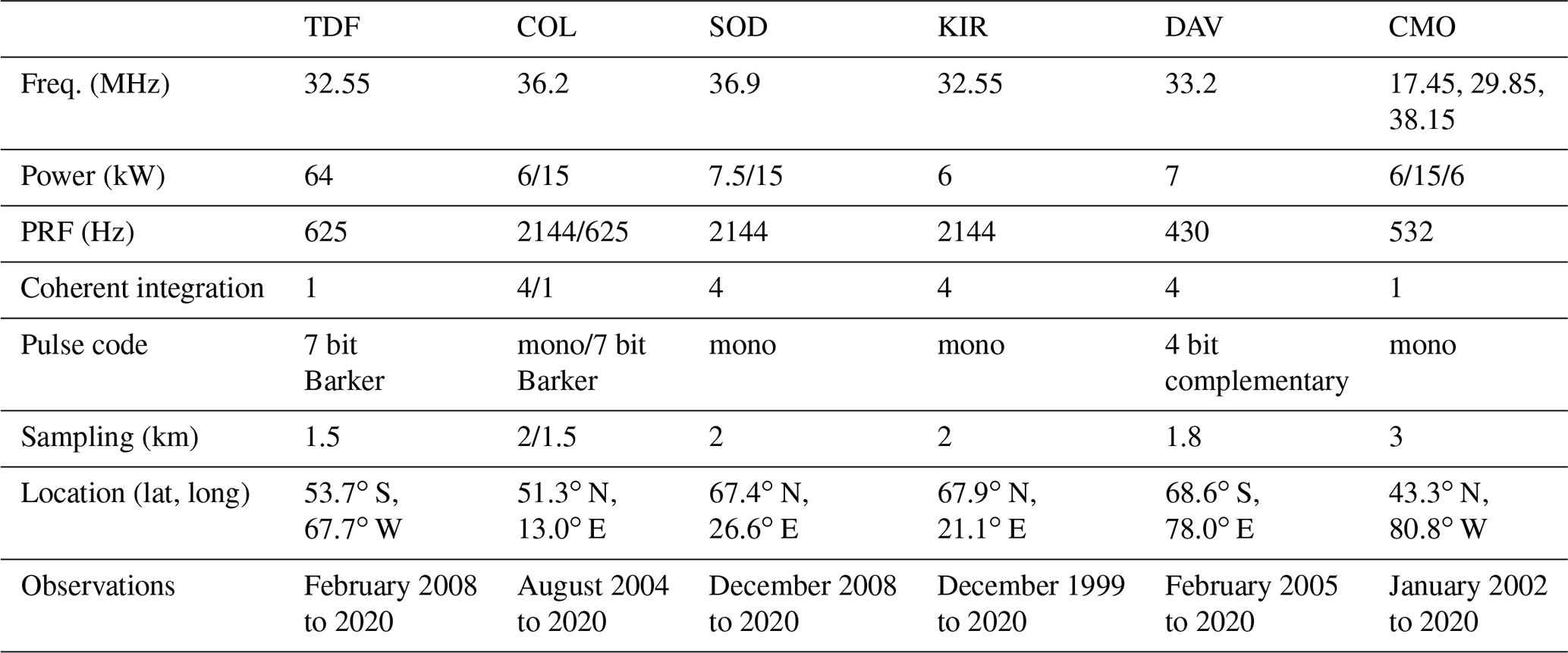
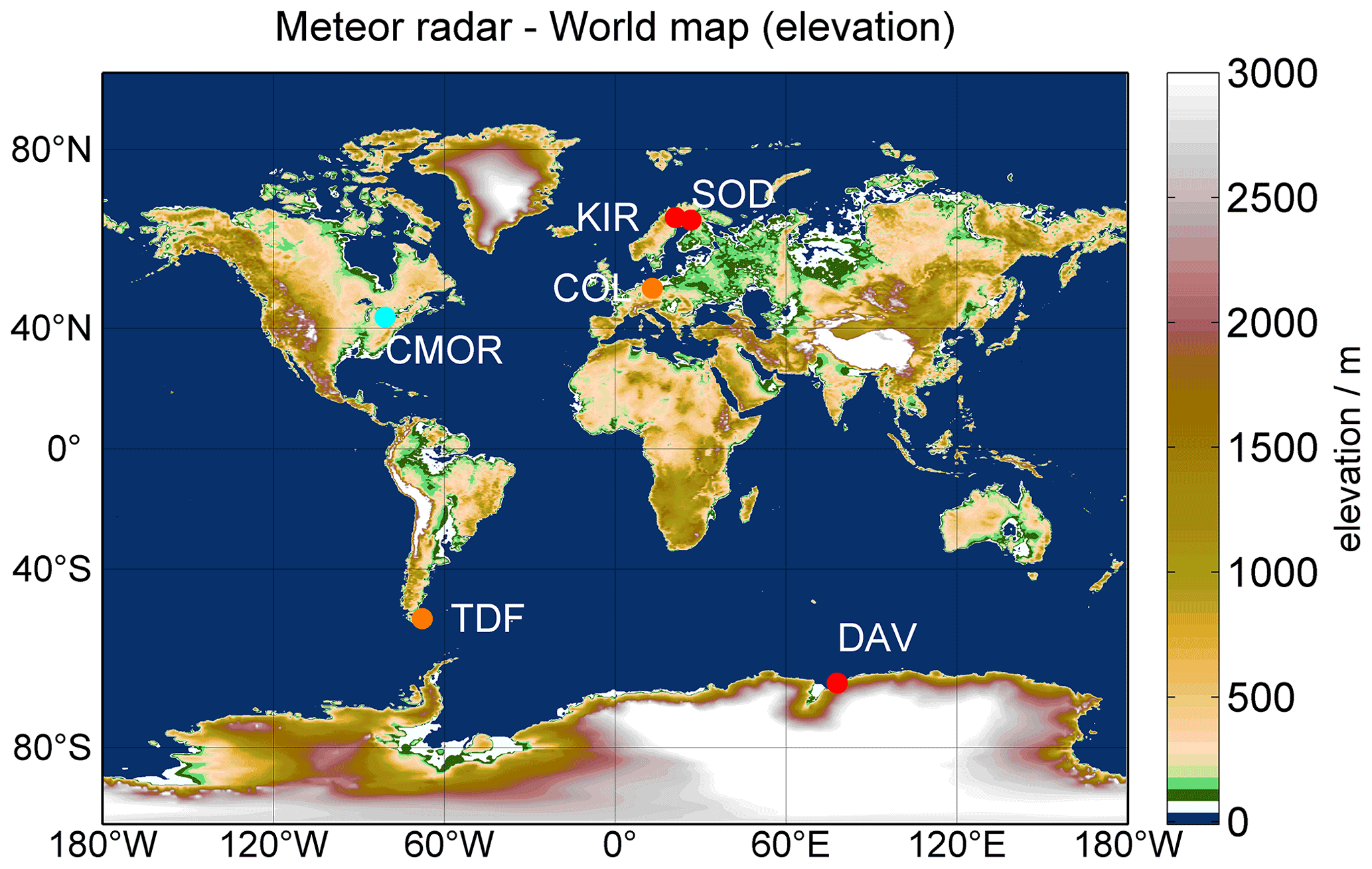
Figure 1World map with meteor radar locations and color-coded mean elevation. Conjugate latitude stations are indicated by the same colors. The plot was generated from etopo1 using the m_map package (Amante and Eakins, 2009).
Meteor winds are computed from so-called meteor position data (Hocking et al., 2001; Holdsworth et al., 2004). We applied harmonized data processing to generate homogeneous wind time series for all sites. The wind retrieval is described in more detail in Stober et al. (2018) and was validated against meteorological analysis NAVGEM-HA (Navy Global Environment Model – High Altitude) (McCormack et al., 2017; Stober et al., 2020a). NAVGEM-HA meteorological analysis utilizes a sophisticated 4D-Var data assimilation scheme, which assimilates observations including mesospheric data from MLS and SABER (Kuhl et al., 2013; McCormack et al., 2017; Eckermann et al., 2018). Given the remarkable agreement between NAVGEM-HA and the meteor radar winds for the general seasonal morphology and the short-term variability, we consider the meteor radar winds to be a proper validation reference for the WACCM-X, GAIA, and UA-ICON wind fields.
2.2 GAIA
GAIA is a 3D, self-consistent, fully coupled, whole-atmosphere model of the Earth's troposphere, stratosphere, mesosphere, thermosphere, and ionosphere covering the altitude range from the ground to ∼600 km for the neutrals and to 3000 km for the plasma (Jin et al., 2012). It has a horizontal resolution of (latitude × longitude) and a vertical resolution of 0.2 scale heights. The model uses parameterizations to account for gravity waves (GWs), with formulations by McFarlane (1987) for orographic GWs and by Lindzen (1981) for non-orographic GWs. In the troposphere, stratosphere, and mesosphere, a full radiation scheme developed by Nakajima et al. (2000) is used. The simulated atmosphere parameters (e.g., wind, temperature) are given in hourly values. GAIA has been demonstrated to be particularly good at capturing comprehensive coupling processes between the lower and upper atmosphere at different temporal and spatial scales, e.g., the wave-4 structure and the thermosphere cooling during sudden stratospheric warmings (SSWs) (H. Liu et al., 2009; Liu et al., 2014).
This study uses the same 21-year-long reanalysis data-driven simulation results as those used for the ENSO study in Liu et al. (2017). Briefly, A nudging technique is used to constrain the model output (e.g., pressure, temperature, wind) below 30 km of altitude to the reanalysis data JRA-25/55 by the Japan Meteorological Agency with a spatial resolution and a 6 h temporal resolution (Onogi et al., 2007; Kobayashi et al., 2015). Due to the update of JRA-25 to JRA-55 in 2014, the simulation uses JRA-55 for 2014–2016 and JRA-25 before that. The F10.7 index as a proxy for the EUV input was set to observed values, while a fixed cross-polar-cap potential of 30 kV and a quiet particle precipitation condition were held throughout the simulation period to exclude any geomagnetic activity effect.
2.3 WACCM-X(SD)
The Whole Atmosphere Community Climate Model Extension (WACCM-X) is one of the atmosphere configurations of the Community Earth System Model (CESM; Hurrell et al., 2013). WACCM-X models the whole atmosphere from the lower boundary (representing ocean, land, or ice) to the upper boundary in the thermosphere (500–700 km of altitude depending on solar activity). Representation of the atmospheric physics in WACCM-X up to the lower thermosphere (∼130 km of altitude) is similar to that of the conventional WACCM configuration (Marsh et al., 2013), while representation of the ionospheric electrodynamics is similar to the Thermosphere–Ionosphere Electrodynamics General Circulation Model (TIE-GCM; Richmond et al., 1992; Maute, 2017). Development and validation of the WACCM-X are described by Liu et al. (2018)1.
The Specified Dynamics (SD/WACCM-X) simulation run deployed here (Gasperini et al., 2020) constrains tropospheric and stratospheric dynamics up to ∼50 km of altitude using reanalysis based on the Modern-Era Retrospective Analysis for Research and Applications (MERRA; Rienecker et al., 2011). We refer to this run further on as WACCM-X(SD). A more detailed description of the nudging procedure is given in Smith et al. (2017). The simulated atmospheric dynamics including zonal and meridional winds with 3 h time resolution are given on the pressure levels with scale height vertical resolution above the upper stratosphere and uniform horizontal resolutions in latitude and longitude of 2.5 and 1.9∘, respectively. The effects of non-orographic gravity waves (GWs) are parameterized using the source-oriented parameterization approach (Richter et al., 2010; Garcia et al., 2017). Orographic GWs are parameterized according to McFarlane (1987). The external forcing due to varying geomagnetic activity is parameterized using the planetary Kp index with the high-latitude plasma convection specified according to Heelis et al. (1982).
2.4 UA-ICON
The Upper Atmosphere ICOsahedral Non-hydrostatic (UA-ICON; Borchert et al., 2019) GCM covers the atmosphere from the surface to 150 km and is a vertical extension of the standard ICON configurations, which usually have the lid at about 80 km. ICON is available with different physics packages to be used for numerical weather prediction (Zängl et al., 2015) and climate studies (Giorgetta et al., 2018; Crueger et al., 2018). The upper atmosphere extension can be run with both physics packages. Here we make use of the latter. The upper atmosphere configuration extends the dynamical core from shallow- to deep-atmosphere dynamics and includes an upper atmosphere physics package with parameterizations for molecular diffusion, radiation in the Schumann–Runge bands and continuum, extreme UV, non-LTE effects (LTE: local thermal equilibrium) and NO cooling, and chemical heating (see Borchert et al., 2019, for details). The latter is necessary as UA-ICON does not calculate air chemistry interactively but uses prescribed climatologies of radiatively active species. Furthermore, UA-ICON uses all physics parameterizations from the standard configuration as described by Giorgetta et al. (2018), including in particular parameterizations for effects from non-orographic gravity waves (Hines, 1997) and sub-grid-scale orography (Lott, 1999). ICON uses a triangular horizontal grid derived from a spherical icosahedron by subdivisions of triangular cells. Here we make use of a so-called R2B4 grid with a horizontal resolution of about 160 km. In the vertical, ICON uses a terrain-following hybrid sigma height grid with 120 layers in this case. Rayleigh damping of vertical winds is applied above 120 km. The simulation presented here uses the same model configuration as the climatological test case described by Borchert et al. (2019). It has been run with climatological present-day-like boundary conditions for 21 years with the first year discarded as spin-up. In contrast to the GAIA and WACCM-X(SD) experiments, the meteorology in the UA-ICON simulations has developed freely as no nudging technique has been applied.
Comparing model fields and observations is very often not as straightforward as expected as the model data usually have a different spatial and temporal resolution than the observations. Thus, in a first step we performed a data reduction for the WACCM-X(SD), GAIA, and UA-ICON global data sets by cutting out all grid points in the vicinity of the meteor radars using a 300 km radius, which is a bit more than the actual beam width used in the wind retrieval of about 220 km radius, but it ensures that at least five grid points are available from each model and for each site. We extracted for each meteor radar location the geopotential height, the zonal and meridional wind, temperature, and pressure for all grid points that fall within the abovementioned area around the meteor radars. These reduced data sets are now further analyzed to simulate meteor radar observation. Therefore, we converted the geopotential heights (Φ) into geometric altitudes (h) for each extracted profile using the expression by taking into consideration variable gravity.
Here, REarth(lat,long) corresponds to the Earth radius at a given latitude and longitude. In a next step, the converted height vectors for each profile are interpolated to a reference altitude vector, which has a vertical resolution of 2 km between 16 and 150 km, 5 km vertical resolution at altitudes from 155–200 km, 10 km vertical resolution between 210 and 300 km, and a 20 km vertical resolution at altitudes above 320 km to account for the decreased model resolutions due to the pressure level spacing in the models. Finally, we compute the median and variance for all profiles and obtain a mean zonal and meridional wind and temperature corresponding to the observation volume of each meteor radar. Furthermore, we derive the variance of these parameters, which provides a proxy for the statistical uncertainties similar to the meteor radar observations. The final result of our data reduction is time series of zonal and meridional winds with a temporal resolution of 1 h for GAIA and UA-ICON and 3 h for WACCM-X(SD), respectively, and a 2 km vertical resolution at the mesosphere–lower thermosphere, which is identical to the meteor radar observations.
MR winds are obtained using the retrieval algorithm described in Stober et al. (2018), which is basically a further evolution of Hocking et al. (2001) and Holdsworth et al. (2004). The retrieval includes a full Earth geometry based on the WGS84 reference ellipsoid, full nonlinear error propagation, and a spatiotemporal Laplace filter as a Tikhonov regularization constraint. Furthermore, the wind retrieval does not require w=0 and explicitly fits for the vertical component, which is considered to be remaining wind bias due to the lack of independent validation sources. However, these vertical winds have proven to provide a good quality control and show a Gaussian distribution with a width of w±0.25 to ±0.35 m s−1 around the zero wind line. The benefit of this retrieval is that we obtain for all systems a harmonized wind time series based on the same quality control criteria.
Atmospheric mean winds and tides are analyzed using the ASF, which is described in more detail in Baumgarten and Stober (2019) and Stober et al. (2020b) and was already applied in several studies (Stober et al., 2017, 2021a; Pokhotelov et al., 2018; Wilhelm et al., 2019) to decompose MR winds in daily mean winds as well as diurnal and semidiurnal tides for the zonal and meridional components, respectively. The technique is implemented based on least square fits with full error propagation, which permits us to apply the algorithm to unevenly sampled data with data gaps. Similar to wavelets the window length is adapted for each of the fitted wave periods (Torrence and Compo, 1998). Furthermore, we minimize the impact of inertia-scale gravity waves on the tidal analysis by applying a vertical regularization to the tidal phases. Stober et al. (2021a) show an example comparing the ASF2D with classical harmonic analysis for different window lengths. Due to the intermittent and nonstationary wave field generated by gravity waves and tides, long window lengths tend to produce artifacts and leak energy between the different wave scales. Furthermore, the meteor radar sampling is irregular in time, which additionally introduces spectral leakages that are significantly reduced by the ASF2D technique.
The GAIA, WACCM-X(SD), UA-ICON, and MR time series are analyzed with the same ASF2D algorithm to ensure the best possible comparability and to minimize differences, which might be introduced when different analysis procedures are applied. Thus, we obtain harmonized time series for daily mean winds, diurnal and semidiurnal tidal amplitudes and phases, and a gravity wave spectral residuum for each data set. The model data are available with different temporal resolutions, which refers to the cadence of the data output of the meteorological fields rather than the actual numerical temporal step size (e.g., WACCM-X(SD) is solved with 5 min resolution). Hence, the model data for each temporal step represent the numerical solution for this output period and not a temporal average as in the observation. Furthermore, we performed an additional test to ensure that the coarser temporal resolution of WACCM-X(SD) of 3 h has no impact on the harmonized time series. Thus, we used an earlier version WACCM-X (v.1.9) run with hourly data output for cross-validation and found no resolution-dependent issues.
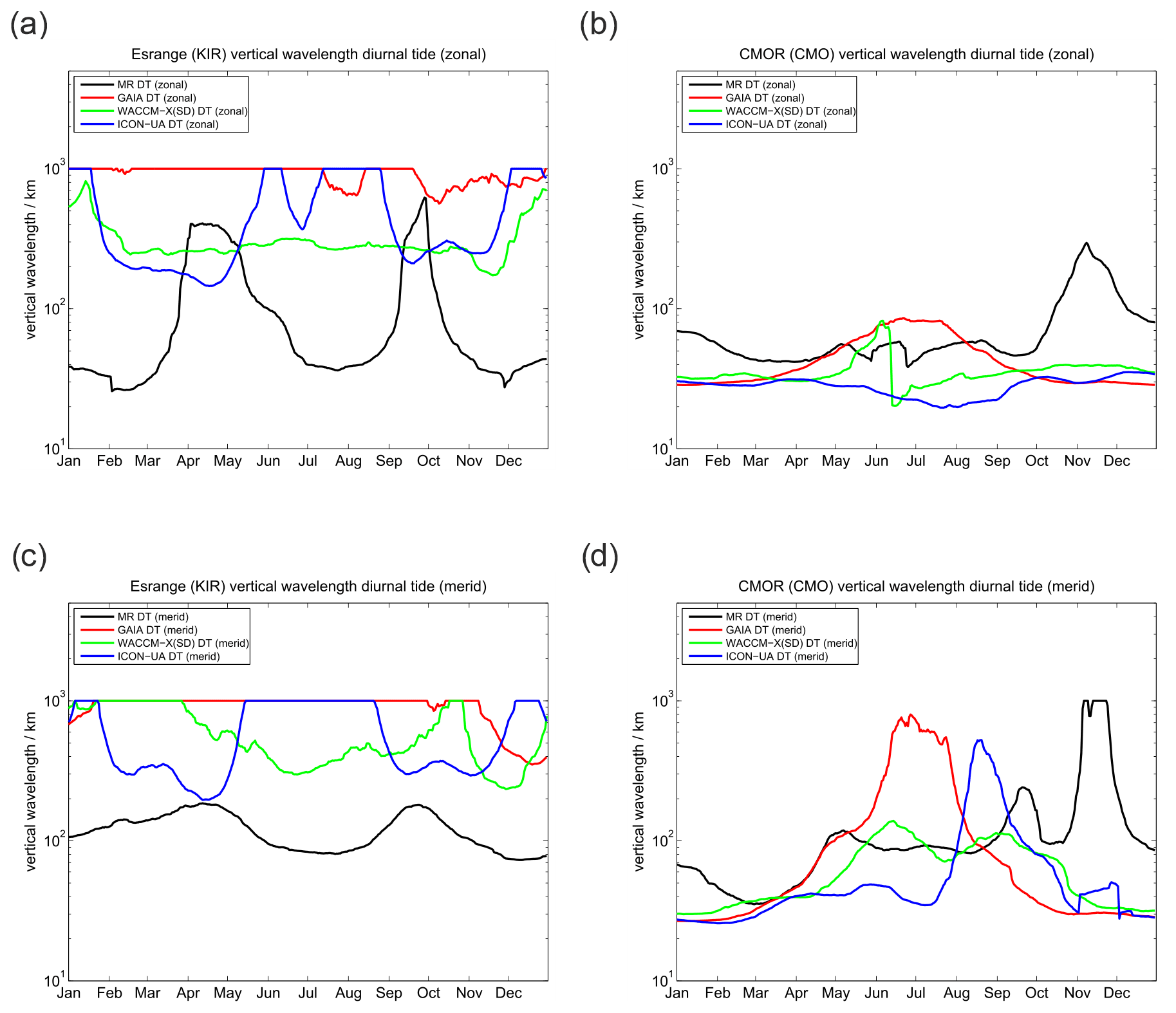
Vertical wavelengths of the diurnal and semidiurnal tides are also estimated from the vertical phase profiles. Therefore, we estimated the instantaneous vertical linear slope of the unwrapped phases in the altitude range between 80 and 100 km. The vertical wavelength is then estimated from the altitude difference between the −π and π phase transitions. This method allows us to derive vertical wavelengths that are much longer than the actual width of the meteor layer. Such long vertical wavelengths correspond to evanescent tidal modes. However, we did not define a certain threshold but consider vertical wavelengths that are much longer than 300 km to be evanescent or not vertically propagating. Vertical wavelengths of the diurnal tide were truncated at 1000 km for plotting reasons. Semidiurnal tides only occasionally showed such long wavelengths and are thus presented without truncation.
4.1 Mean winds
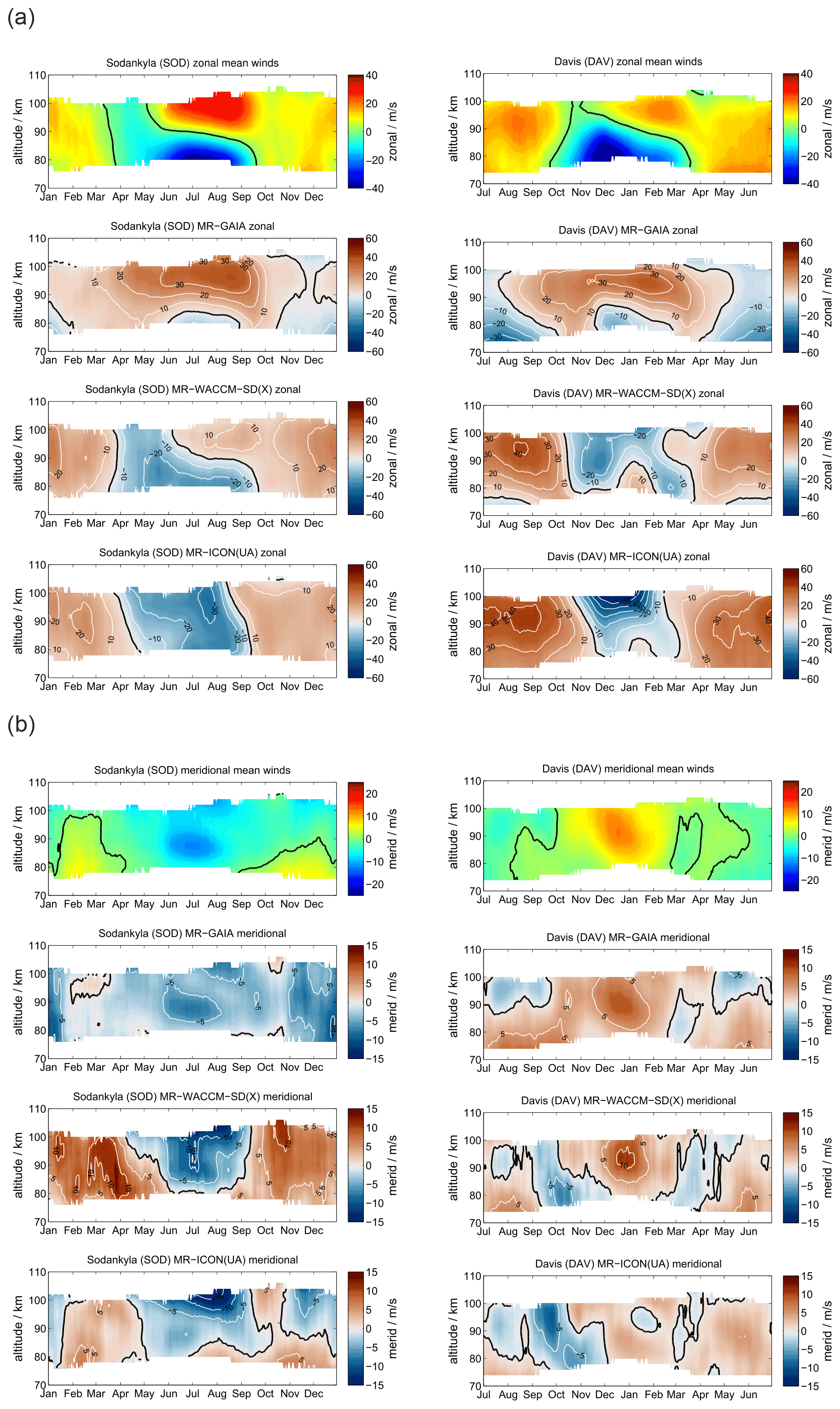
SOD and DAV are located at conjugate latitudes in Arctic and Antarctic sectors, respectively. Figure 2 shows a comparison of the meteor radar observations of zonal and meridional daily mean winds. Panel (a) presents the zonal component for SOD (left column) and DAV (right column). The upper row visualizes the meteor radar measurements, the second row shows GAIA, the third row shows WACCM-X(SD), and the lower row shows UA-ICON.
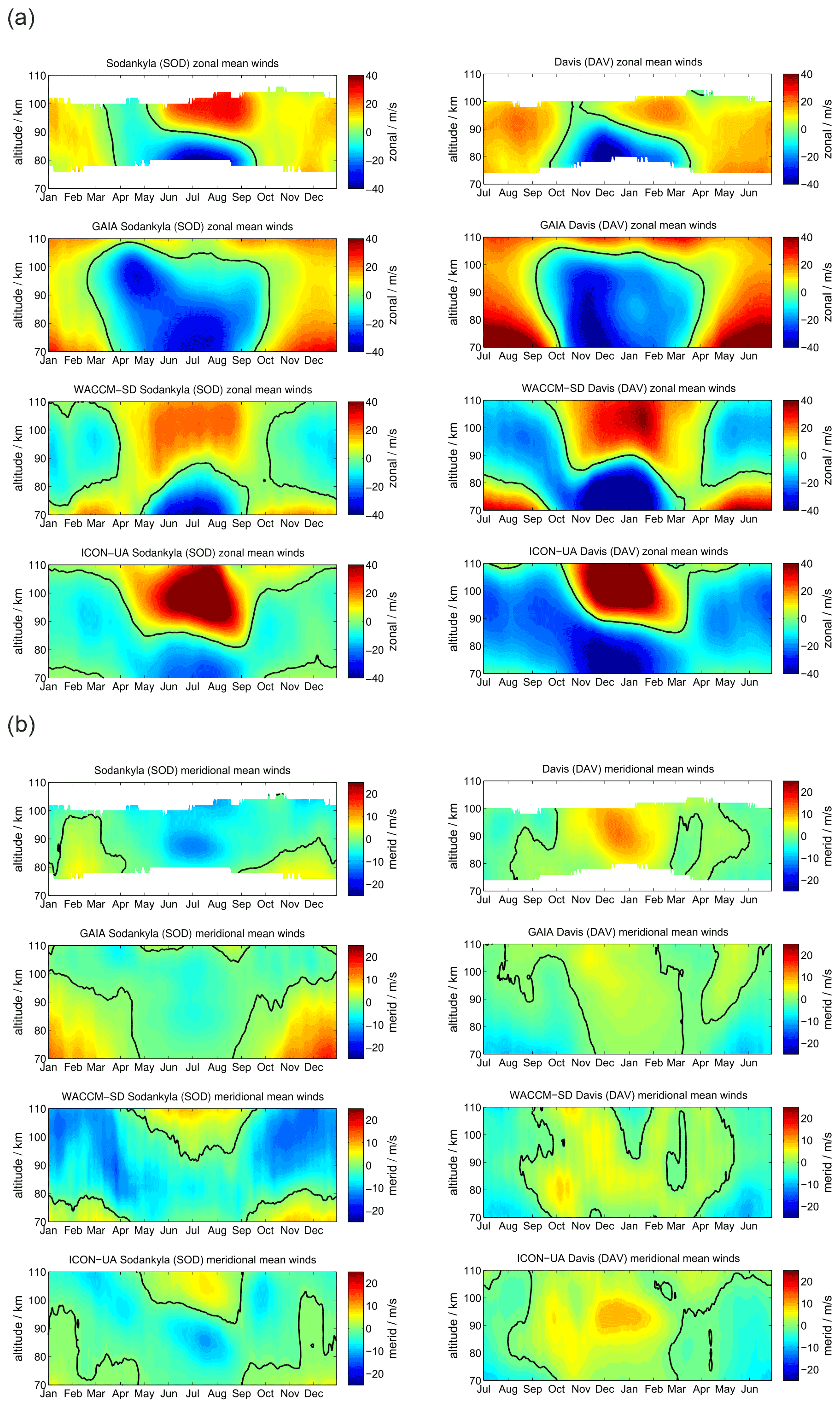
Figure 2Comparison of zonal (a) and meridional (b) daily mean winds for the MRs at SOD (left column) and DAV (right column). The winds for Davis are shifted by half a year.
Zonal winds exhibit a characteristic seasonal pattern with weak eastward winds during the hemispheric winter and a wind reversal from westward to eastward winds with a gradual change in the reversal altitude over the hemispheric summer months. Furthermore, there is a characteristic asymmetry of the spring transition compared to the fall. The SOD MR observes westward winds from mid-March to May at altitudes up to 100 km, whereas the corresponding structure at DAV shows near zero wind at 100 km in October–November and a much stronger westward wind enhancement at approximately 90 km of altitude. Another major difference between the Northern and Southern Hemisphere is the strength of the eastward winds above the summer mesopause, which are stronger in the Northern Hemisphere at SOD. On the other side, the eastward winds during the winter months exhibit higher velocities in the Southern Hemisphere.
GAIA reproduces some features of the seasonal morphology of the zonal wind. Mainly, the model shows eastward winds during the hemispheric winter season with a similar magnitude as the MR measurements at SOD and DAV. However, the summer wind reversal occurs at altitudes 10–15 km higher compared to the observations. Furthermore, GAIA does not indicate an eastward wind enhancement in the shown altitude range. Another interesting feature of GAIA is that the seasonal asymmetry of the spring and fall transition is visible in the model data. Interhemispheric differences are also shown by the model. The southern hemispheric wind speeds are increased by 5–8 m s−1 compared to their northern hemispheric counterparts.
The seasonal morphology in WACCM-X(SD) shows substantial differences from the MR measurements during the hemispheric winter months: the zonal wind changes from eastward to westward between 70 and 80 km and remains westward at most MLT heights, whereas observational data show no reversal and are eastward in this region. In terms of the summer wind reversal from westward to eastward, winds can be found in the model and in the observations. As such, the general seasonal morphology tends to be more symmetric in WACCM-X(SD). The spring and fall transitions look very similar. The summer mesospheric wind reversal does not exhibit the gradual descent of the reversal altitude. Southern hemispheric winds at DAV show increased magnitudes compared to the observations. The zonal wind pattern is thus not well-represented during winter months in both hemispheres for SOD and DAV in WACCM-X(SD). Similarly to WACCM-X(SD), UA-ICON does not reproduce westward winds during the winter months. It also indicates even stronger eastward winds in both hemispheres during the summer months. Furthermore, it is noticeable that UA-ICON tends to capture the seasonal asymmetry in the zonal winds and shows a gradual decrease in the summer wind reversal altitudes, as is seen in the observations. Meridional winds are compared in Fig. 2b. MRs at conjugate latitudes are supposed to have rather similar qualitative agreement of the seasonal pattern but with a 180∘ phase shift considering the residual circulation (Becker, 2012). SOD and DAV show northward winds during northern hemispheric winter and southward winds during the summer, reflecting the hemispheric upwelling above the summer pole and the downwelling during the winter months.
GAIA exhibits a very similar seasonal characteristic for both stations. However, the northward winds during the northern hemispheric winter have an increased magnitude compared to the observations at SOD and are less strong above DAV. Nevertheless, GAIA is capable of capturing the main seasonal features in the meridional component for both locations.
Comparing meridional winds in WACCM-X(SD) with the observations reveals distinct differences between the conjugate latitudes. In the Southern Hemisphere above DAV the seasonal morphology is well-reproduced in WACCM-X(SD) and shows the northward winds during the northern hemispheric winter and southward winds during May to August. This is not the case for SOD: WACCM-X(SD) shows an entirely different seasonal meridional wind throughout the year, which is southward at the altitude range between 80 and 100 km most of the time. Furthermore, the model exhibits a wind reversal from southward to northward during the summer months in May to September above 100 km, which is not indicated in the observations. Meridional winds in UA-ICON again show a seasonal characteristic similar to WACCM-X(SD). However, the magnitude of the meridional winds appears to be in better agreement with the observations. In particular, the meridional winds at DAV look similar compared to the observations.
A more qualitative comparison is estimated by computing absolute differences between the MR climatologies and the models. Therefore, we use the MR measurements as a reference and subtract the model output. Bluish colors indicate an overestimation of the model data, and reddish colors support an underestimation. Absolute differences between the daily zonal and meridional MR winds and the corresponding model fields are shown in Appendix B1. The zonal wind component exhibits winter differences of about 40 m s−1 and summer offsets of about 30 m s−1. There is a tendency for the absolute values to be larger in the Southern Hemisphere for SOD and DAV. Meridional winds indicate mean differences of for GAIA and ICON-UA. Only WACCM-X(SD) occasionally shows more than a 10 m s−1 offset.
4.2 Diurnal tides
At polar latitudes diurnal tides gain only moderate amplitudes, although they are still visible throughout the year, which is also predicted from the Laplace tidal equation and the corresponding Hough modes (Andrews et al., 1987; Wang et al., 2016). The amplitudes reach their largest values during the hemispheric summer months. Furthermore, the zonal and meridional amplitudes show consistent seasonal patterns. Typically, at middle and high latitudes the meridional amplitudes exceed the zonal amplitudes during the summer months as documented before (Portnyagin et al., 2004; Jacobi, 2012; She et al., 2016; Wilhelm et al., 2017; Baumgarten and Stober, 2019; Pancheva et al., 2020). Figure 3 presents the comparison between SOD and DAV with a similar arrangement of the panels as for the mean winds. The MR observations reveal a characteristic vertical structure of the diurnal tidal amplitude for the hemispheric summer months, which shows a first enhancement at altitudes below 80 km and a second maximum above 95–100 km. Furthermore, there is a second hemispheric winter maximum apparent at DAV during June and July at altitudes below 80 km, which is less obvious at SOD.
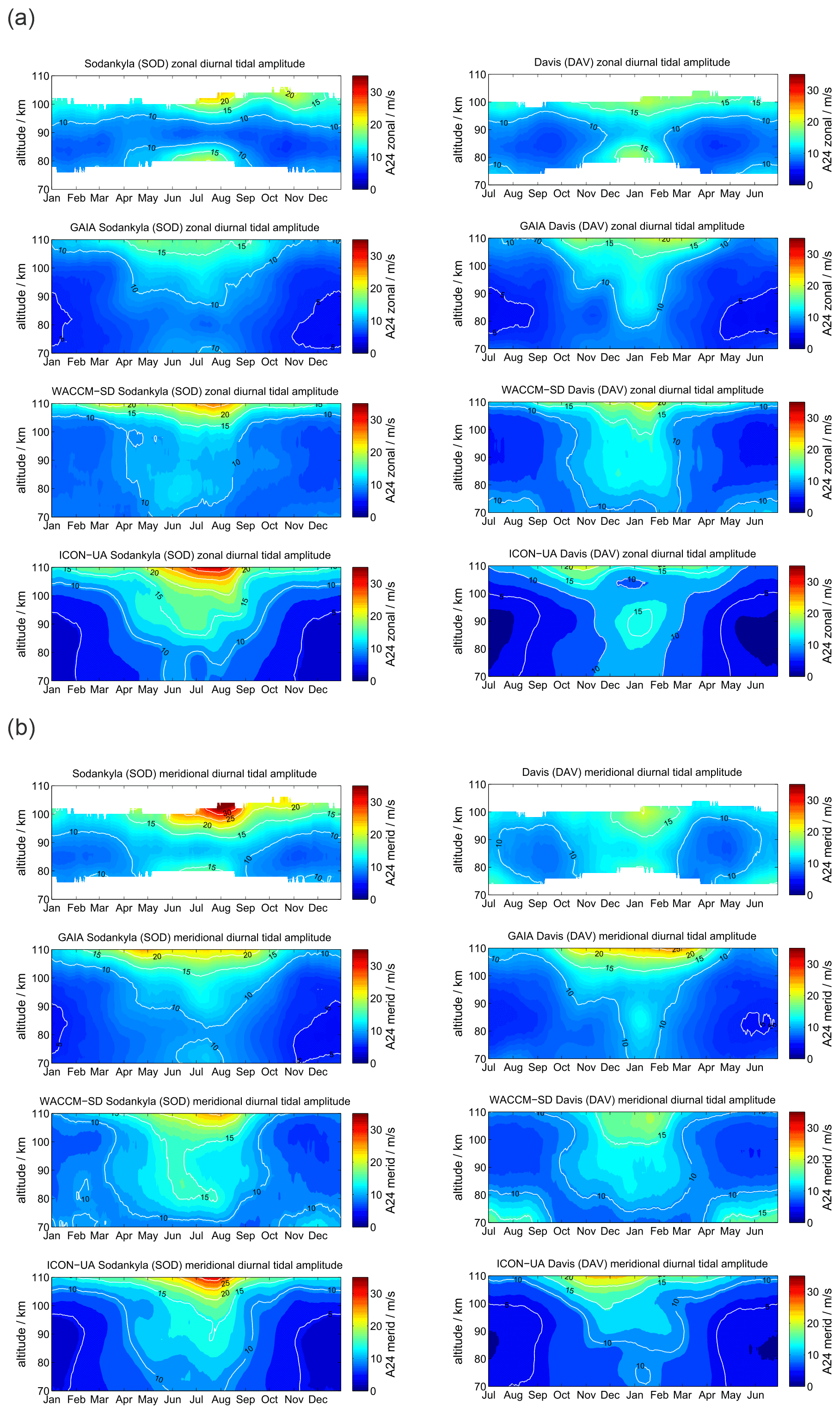
GAIA and UA-ICON capture most of the seasonal characteristic of the diurnal tidal amplitudes above 90 km but show no tidal enhancements below 80 km. The meridional amplitudes are also more amplified compared to the zonal component in both hemispheres, which is consistent with the observations. However, the vertical structure of diurnal amplitudes is less visible relative to the observations. This is also the case for WACCM-X(SD). WACCM-X(SD) also shows the diurnal tidal enhancement above DAV during the hemispheric winter below 80 km, which is not found in GAIA and UA-ICON. However, in WACCM-X(SD) this lower amplitude maximum is stronger than amplitudes above 100 km during the same period, which appears to be reversed compared to the observations. In general the amplitudes of the diurnal tide appear to be almost equal in the zonal and meridional component for DAV, which is also reflected by all three models. Only at SOD do the observations indicate enhanced amplitudes in the meridional component, which seems to be less pronounced in all three model outputs. One noticeable aspect of UA-ICON is the diurnal tidal seasonal climatology, which indicates much lower amplitudes during hemispheric winter compared to the observations and the other two models.
Comparing the diurnal tidal phase between SOD and DAV MR observations, we found remarkable differences in the seasonal pattern between the two hemispheres (see Fig. 4). The zonal and meridional diurnal phase at DAV remains more or less stable throughout the year, indicating only little annual variation with longer vertical wavelengths in the meridional component, whereas at SOD a pronounced semiannual structure is observed with distinguished phase changes in April–May and October.
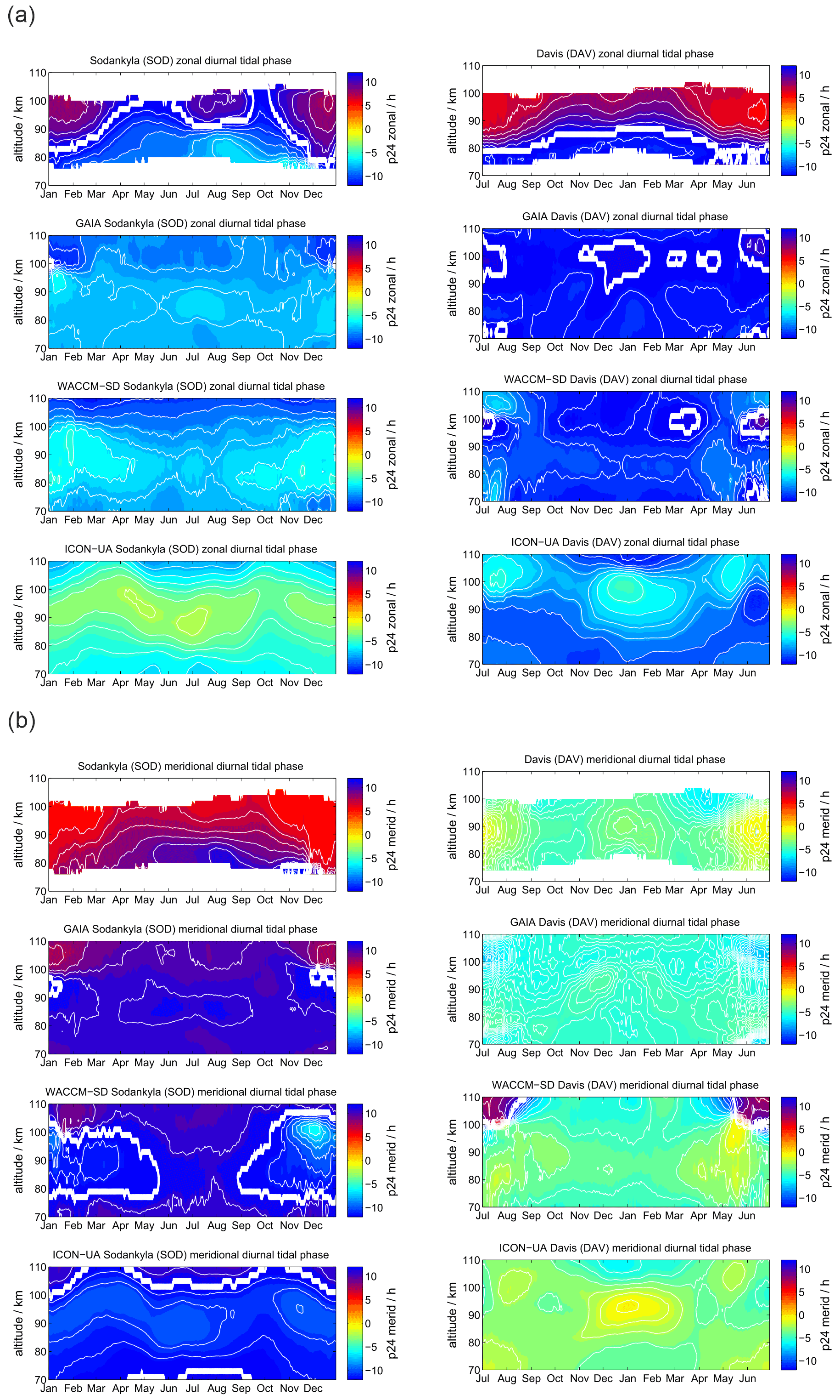
Figure 4The same as Fig. 3, but for the diurnal tidal phases. The white line indicates a phase jump or the zero phase transition.
WACCM-X(SD) and GAIA present a very similar seasonal diurnal tidal phase characteristic for both components, which deviates by several hours relative to the MR measurements at both locations. In this respect, there is less good agreement of the vertical diurnal tidal phase structure for both models in comparison to the observations. For the DAV location the WACCM-X(SD) meridional phase even shows a jump above 100 km, which is not seen in GAIA. UA-ICON diurnal tidal phases exhibit an offset compared to the observations, but the vertical structure appears to be similar to GAIA and WACCM-X(SD).
Vertical wavelengths for the diurnal tide are presented in Fig. 5. All three models tend to overestimate the vertical wavelength compared to the MR observations, which could already be seen in the phase plots. These very long vertical wavelengths reaching more than 1000 km in all models during certain periods practically indicate that the tidal modes are evanescent and not vertically propagating.

Figure 5Comparison of vertical wavelengths of the diurnal tide. The left column shows (a) the zonal and (c) meridional vertical wavelength for SOD. Panels (b) and (d) present the same but for DAV.
We also estimate the absolute difference of the diurnal tidal amplitudes, which are shown in Appendix C1. The models tend to overestimate the hemispheric summer amplitudes at 80–90 km of altitude. Typical differences are about 5 m s−1, and only above 100 km of altitude and for the meridional tidal component does the difference exceed 10–15 m s−1.
4.3 Semidiurnal tides
Semidiurnal tides are the dominating tides at middle and high latitudes at the MLT and reveal a characteristic seasonal structure (Portnyagin et al., 2004; Wilhelm et al., 2019; Pancheva et al., 2020; van Caspel et al., 2020), but they also show significant interhemispheric differences. Figure 6 compares the semidiurnal amplitudes. The panels are arranged as for the diurnal tides. At the location of SOD in the Northern Hemisphere the semidiurnal tidal amplitudes are largest during the winter and autumnal equinox in September. The tides already reach values of more than 20 m s−1 at 90 km of altitude and grow further with increasing altitude up to 35 m s−1. During spring and summer months the semidiurnal amplitudes are the smallest at SOD. In the Southern Hemisphere the seasonal characteristic is apparently different. DAV also shows a maximum of the semidiurnal tide at hemispheric autumnal equinox (April–May), but it remains rather weak during the hemispheric winter from June to August. In contrast to the Northern Hemisphere the semidiurnal tide is enhanced again during the hemispheric spring transition from September to December at altitudes above 90 km.
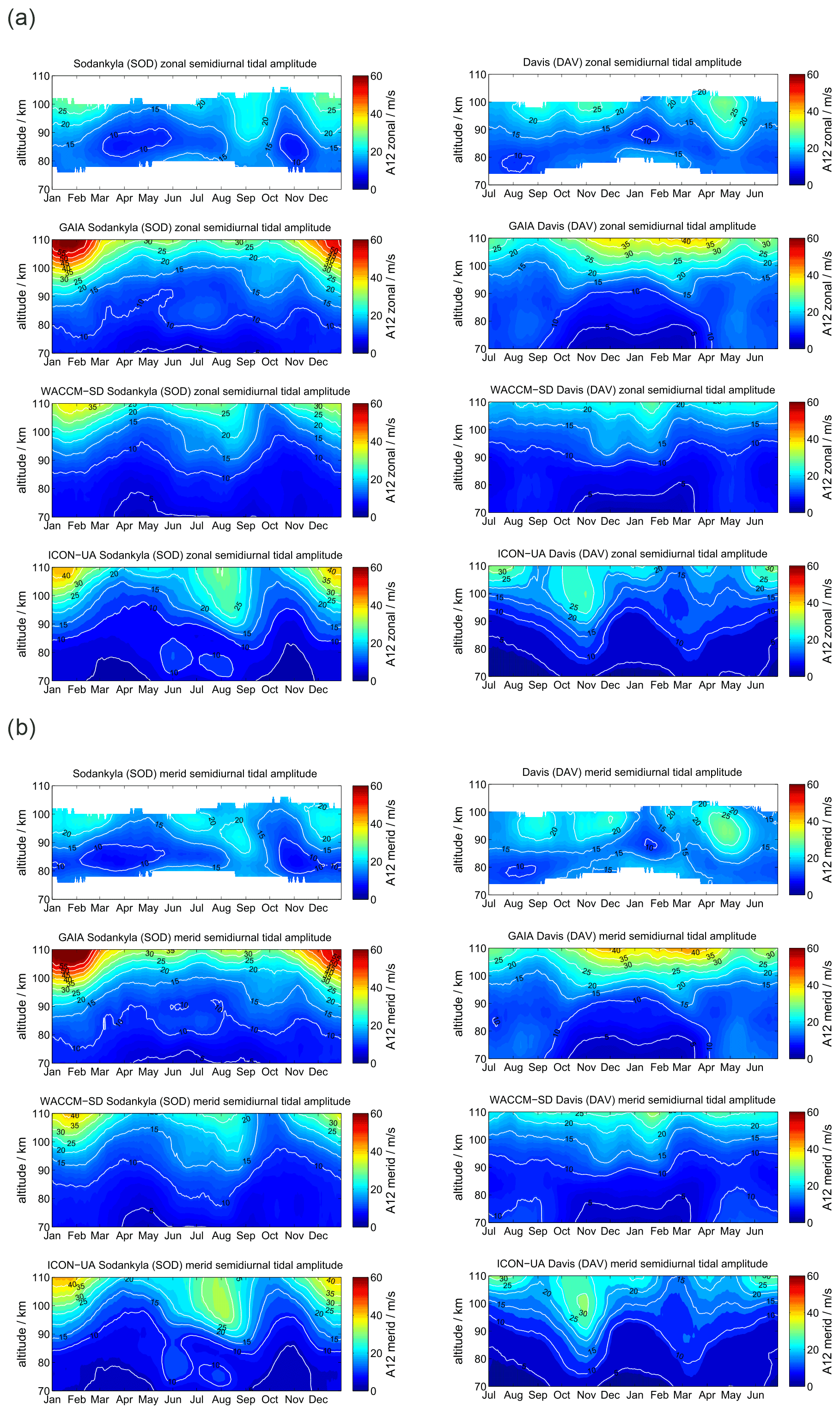
This much more complicated seasonal behavior is only partly reproduced in GAIA, WACCM-X(SD), and UA-ICON. The models show increased semidiurnal tidal amplitudes during the winter months at SOD and DAV, with the largest amplitudes reached in GAIA above 100 km of altitude. The semidiurnal enhancement during the autumnal equinox is basically not present in GAIA in either hemisphere. WACCM-X(SD) indicates an enhancement of the tide for the Northern Hemisphere in both components during August, which is about 1 month too early compared to the MR observations at SOD. UA-ICON indicates a similar seasonal characteristic as WACCM-X(SD) and the observations. The general seasonality of the semidiurnal tidal amplitudes is fairly consistent between the models but exhibits deviations from the observations, which are more significant in the Southern Hemisphere.
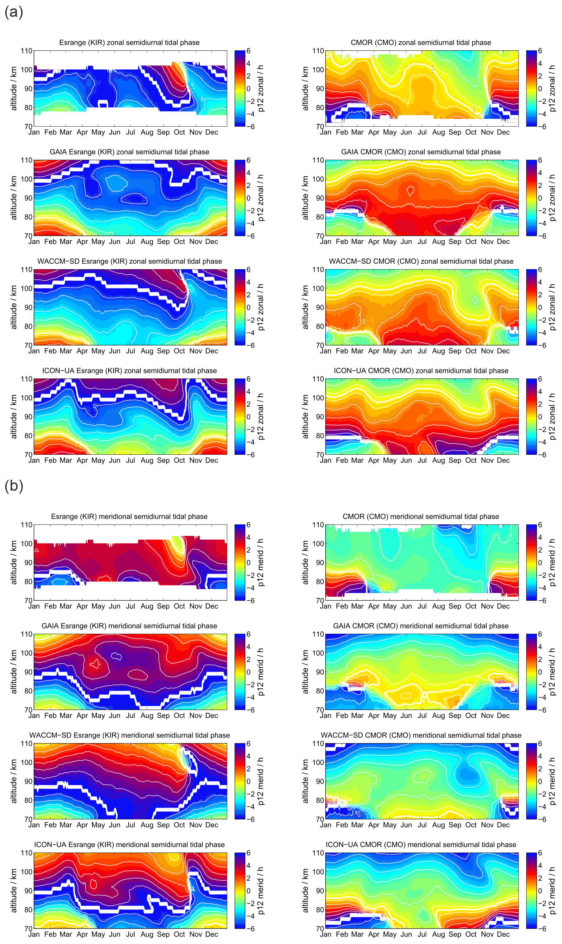
In Fig. 7 we present the semidiurnal tidal phases for SOD and DAV. As already shown for the amplitudes, there are significant interhemispheric differences at polar latitudes. The SOD MR observes a quasi-biannual tidal phase characteristic, whereas at DAV station the annual pattern is more evident. In the Northern Hemisphere the semidiurnal tidal phase basically drifts with season and shows phase variations of several hours through the course of the year. Southern polar latitudes exhibit a much smaller phase variability and more constant seasonal variation of the phase, which is still significant and exceeds several hours, but the changes are not as rapid as in the Northern Hemisphere.
As expected from the diurnal tidal phase analysis, the models have difficulties matching the phase variability and seasonal characteristics, especially in the Southern Hemisphere. GAIA appears to have slightly better agreement with the observations above DAV at altitudes between 80 and 100 km in both components. WACCM-X(SD) indicates a better performance for the Northern Hemisphere and, in particular, captures the phase variability during the fall transition in both components, which is only weakly present in the GAIA data. Surprisingly (taking into account that the model is free-running), UA-ICON semidiurnal tidal phases reproduce the observations for the Northern Hemisphere reasonably well and partly also in the Southern Hemisphere. Similar to WACCM-X(SD), UA-ICON exhibits the rapid phase changes during the northern hemispheric fall transition and shows a bit a more pronounced phase variability during the spring transition.
Semidiurnal tidal amplitude differences are presented in Appendix D1. The semidiurnal tides indicate differences of about 5 m s−1 throughout most of the year for both components and all three models. However, during the fall transition after the end of the hemispheric summer these differences reach up to 15 m s−1. Furthermore, the absolute tidal differences indicate a systematic underestimation of the tidal amplitudes in all three models.

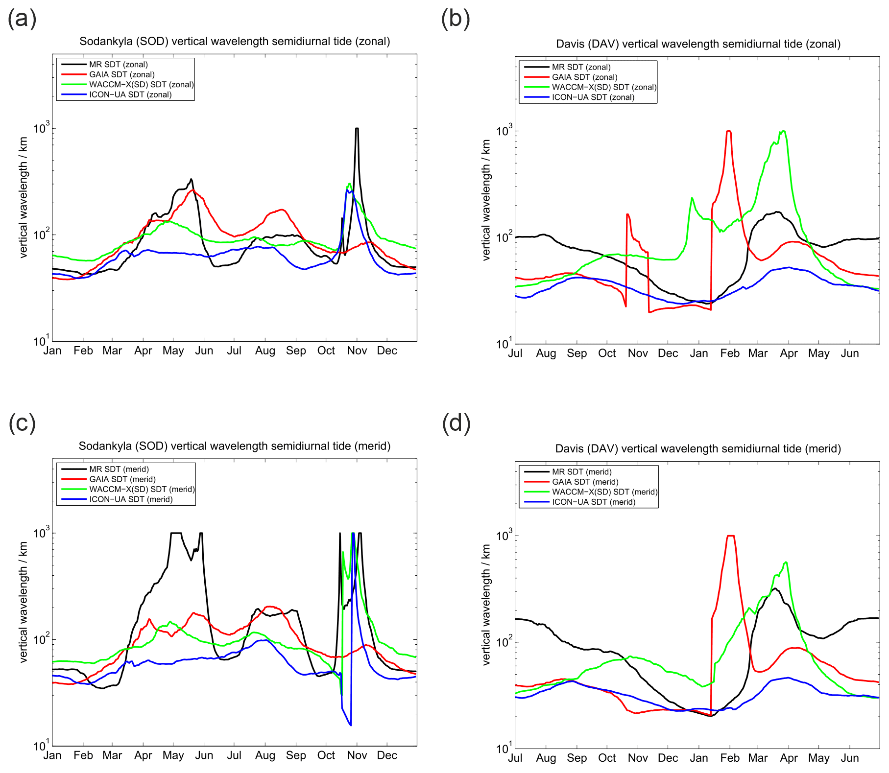
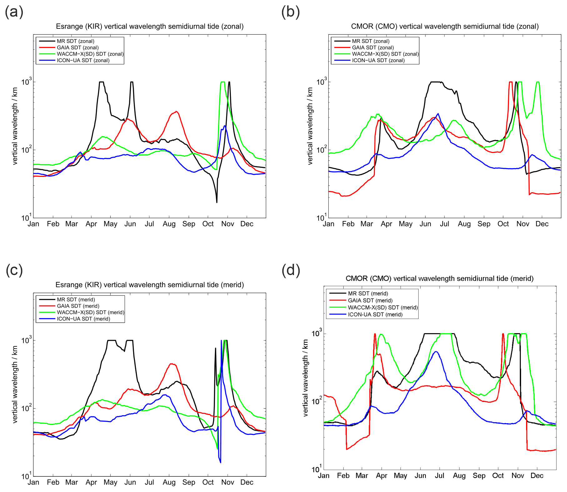
Finally, a comparison of vertical wavelengths of the semidiurnal tide at SOD and DAV is shown in Fig. 8. The first noticeable aspect is the interhemispheric difference of the vertical wavelength between SOD and DAV MR observations. The vertical wavelength appears to be much more variable in the course of the year in the Northern Hemisphere and takes values of about 50–60 km for the winter; there are prominent enhancements during April–June and October–November with values beyond 1000 km. Such large vertical wavelengths actually point to evanescent tidal modes, which essentially do not vertically propagate. From July to September vertical wavelengths of about 100–120 km are observed with the SOD MR. The behavior at the Southern Hemisphere is rather different. During hemispheric summer, short vertical wavelengths of about 25 km are seen above the DAV station, which increase to about 100–120 km during March–April and gradually decrease again afterwards. The very long vertical wavelengths that are found above SOD are missing in the Southern Hemisphere. Similar to the semidiurnal tidal phase, GAIA shows better agreement with the observations at the Southern Hemisphere during the hemispheric winter season from March to October. However, GAIA exhibits two distinct peaks in the vertical wavelength, taking values beyond 1000 km in February and October–November, which are not found in the MR observations at DAV. In the Northern Hemisphere the vertical wavelength seasonal climatology of GAIA is reasonably well-reproduced and the main features such as the triple peak structure are visible, but the model underestimates the vertical wavelengths. WACCM-X(SD) and UA-ICON show some interhemispheric differences and capture the fall transition in the Northern Hemisphere remarkably well, but they underestimate the vertical wavelengths during April–May and July–August. Vertical wavelengths at the DAV station also indicate some systematic deviations from the MR measurements. UA-ICON apparently underestimates the vertical wavelengths compared to the observations and other models during March–April in both hemispheres but otherwise indicates remarkable similarity to the observations and WACCM-X(SD).
5.1 Mean winds
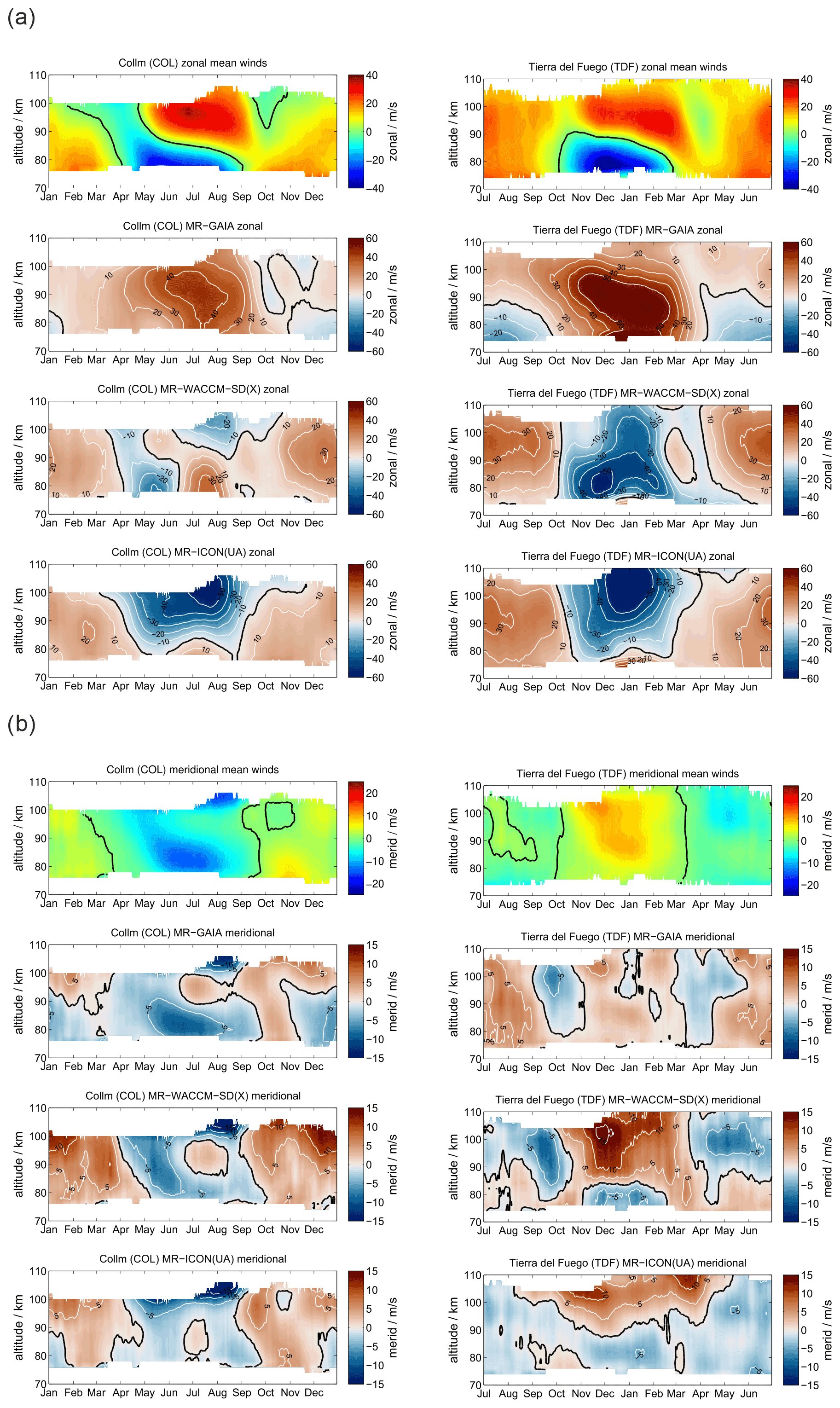
Now we compare the midlatitude stations COL and TDF. Although both stations are at almost conjugate latitudes, they are located in very different geographic regions, which have to be considered. The COL MR station is in the center of Europe and far away from significant orographic mountain wave sources. The Alps are more than 600 km to the southwest, and the Scandinavian mountains are almost 1000 km to the northwest. The TDF MR is much closer to the Andes mountains in Patagonia, which is one of the most relevant mountain wave hot spots on Earth, and thus the observations are directly affected by the mountain wave source and a potential secondary wave forcing up to the mesosphere (Becker and Vadas, 2018; Vadas and Becker, 2018; de Wit et al., 2017).
Figure 9 presents the zonal and meridional daily mean wind climatologies for COL and TDF. As already shown in previous studies (Pokhotelov et al., 2018; Wilhelm et al., 2019), the main difference to the polar latitudes is found at a lower altitude of the summer zonal wind reversal in both hemispheres and a corresponding altitude shift of the meridional southward and northward winds. However, there are some distinct interhemispheric differences between locations and wind components. During the spring and fall transitions zonal winds above 90 km show characteristic differences. TDF observations exhibit eastward winds throughout the year and indicate a weakening of them during the spring and fall period, whereas at COL from March–April until May and in October there is a wind reversal to weak westward winds. Meridional winds have a very similar seasonal characteristic due to the conjugate location of both stations. The meridional wind is always stronger above the stations in the summer hemisphere. Furthermore, the vertical structures are different. The COL MR shows a remarkable vertical structure of meridional southward wind magnitude for the summer months from June to August, which exhibits the highest magnitudes at altitudes corresponding to westward zonal wind. In the Southern Hemisphere, we observe a smoother vertical structure of the meridional wind, which even reverses to northward above 84 km in July and August.
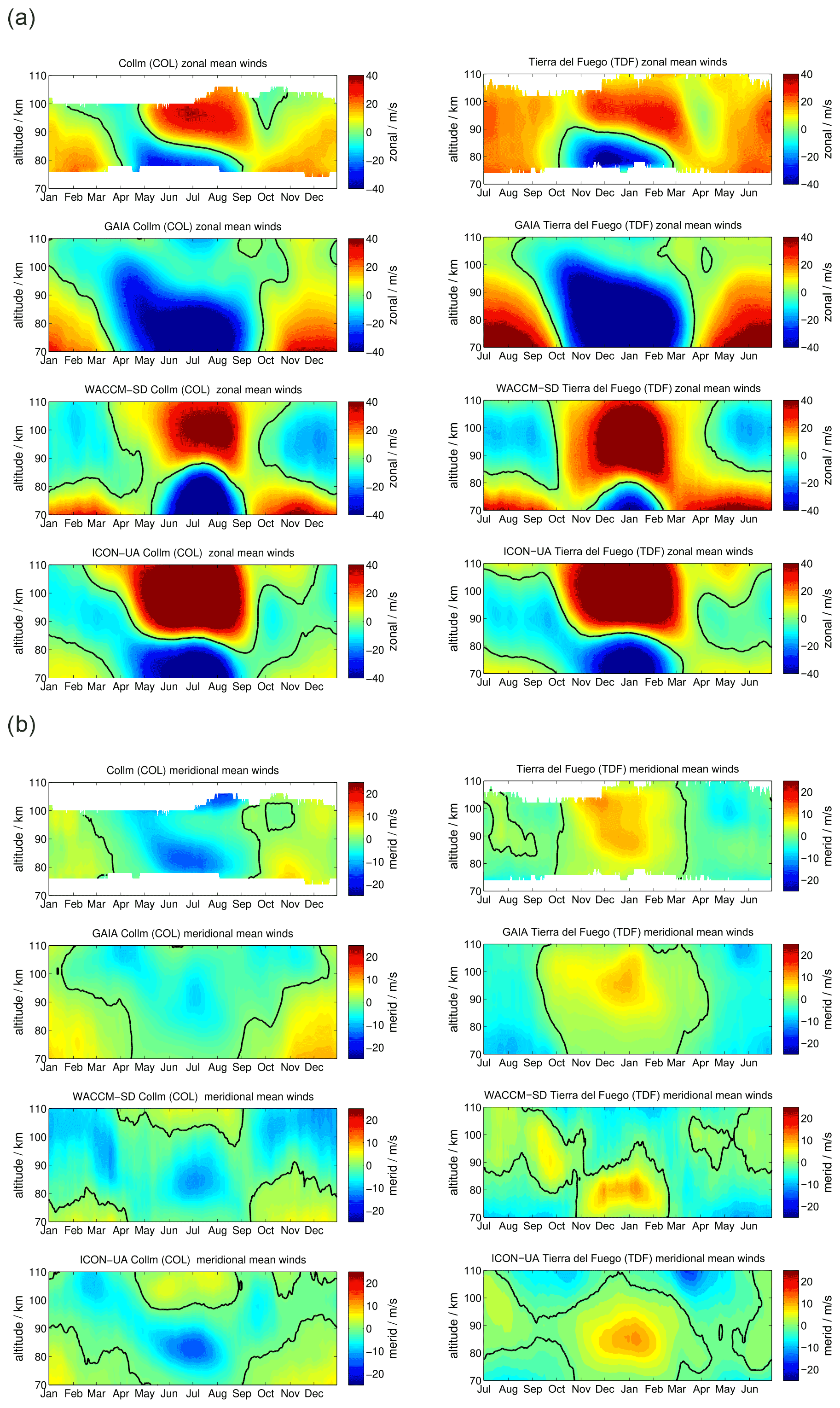
As already found for the polar latitudes, the zonal wind climatologies are only to a certain extent reproduced in the models. GAIA shows better agreement during the winter months, whereas WACCM-X(SD) and UA-ICON exhibit better agreement of the summer zonal wind reversal compared to the MR measurements. All three models tend to overestimate the strength of zonal summer wind systems. The westward winds are too strong and extend to altitudes that are too high in GAIA. WACCM-X(SD) and UA-ICON indicate strong zonal wind reversals at the altitude at which these are found in the observations, but the westward and eastward winds tend to be overestimated. Furthermore, UA-ICON indicates the seasonal asymmetry in the zonal wind, which is a less visible in WACCM-X(SD). GAIA meridional winds and the observations are in better agreement in the Southern Hemisphere compared to the northern midlatitudes concerning their strength and seasonal characteristic. Only the meridional wind reversal in July–August at TDF is not found in the GAIA data. At the northern midlatitudes GAIA shows a more pronounced seasonal structure and underestimates the strength of the meridional southward wind during the summer months, which is likely associated with the summer zonal wind reversal that is not visible in GAIA. In winter, WACCM-X(SD) and UA-ICON exhibit more remarkable differences relative to GAIA and the observations. In the Northern Hemisphere the meridional wind is southward at altitudes between 90 and 100 km throughout the year. Both models apparently only reproduce the seasonality that is found in the observations below 80 km of altitude. In the Southern Hemisphere WACCM-X(SD) and UA-ICON show better agreement during the hemispheric summer months (December–February) but tend to overestimate the wind reversal from southward to northward as well as the seasonal duration compared to the TDF observations.
A comparison of the absolute differences between the models and the meteor radar winds for COL and TDF is shown in Appendix B2. Similar to the polar latitudes, there are rather large differences of about 40 m s−1 in the zonal winds during the hemispheric summer months between the models and the MR observations. These differences are partly due to offsets in the altitude of the summer zonal wind reversal and differences in the strength of the westward and eastward jets. However, during the hemispheric winter months GAIA exhibits mean zonal wind differences of about 10 m s−1. WACCM-X(SD) and ICON-UA indicated offsets of up to 30 m s−1. Meridional winds show typical differences of ±10 m s−1 for GAIA and ICON-UA and occasionally exceed 10 m s−1 for WACCM-X(SD).
5.2 Diurnal tides
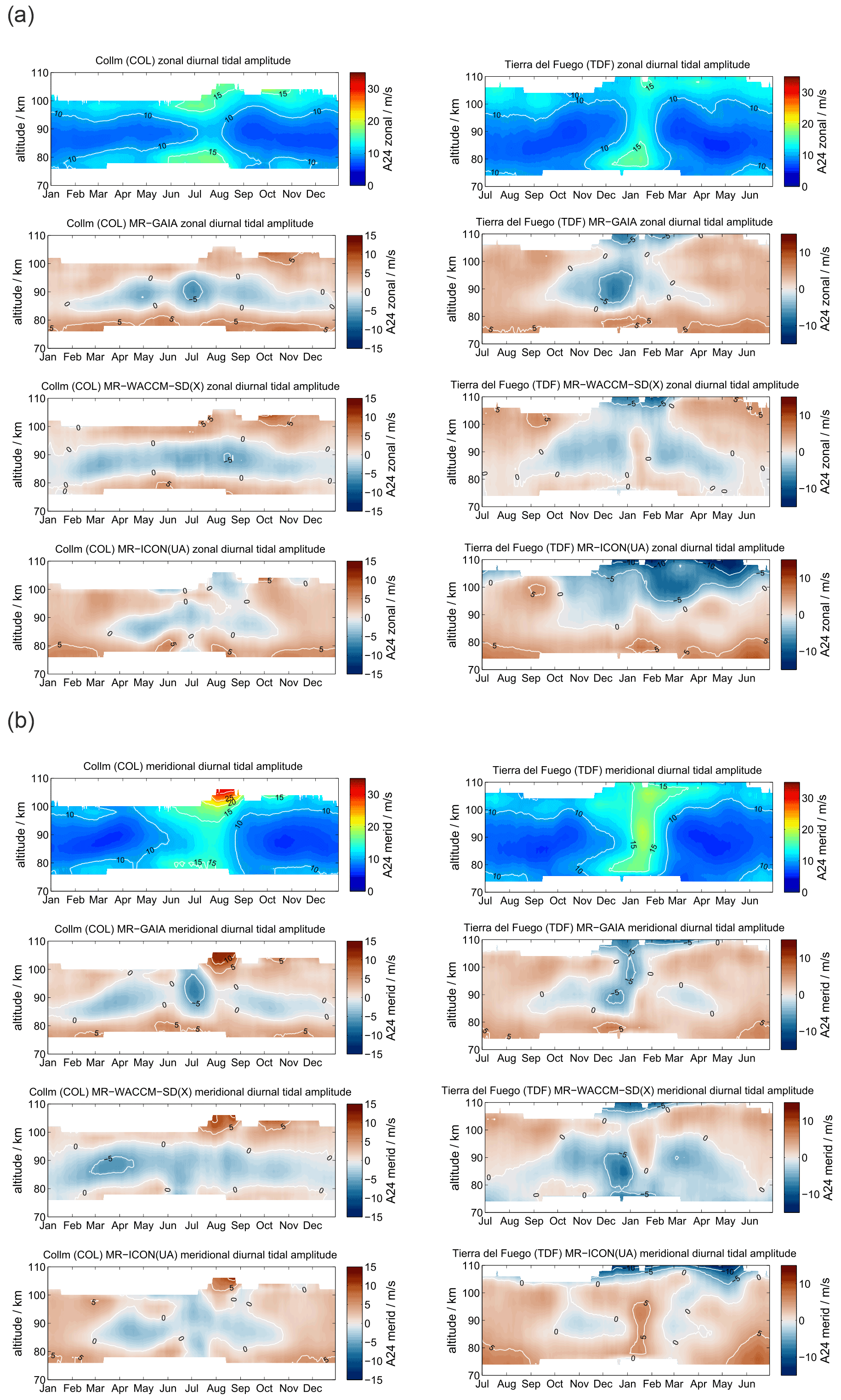
At midlatitudes diurnal tidal amplitudes have a similar seasonal characteristic as at the polar latitudes. During the hemispheric summer season the amplitudes are largest and remain rather small throughout the other months. Figure 10 shows a comparison of the diurnal tidal amplitudes between COL and TDF. Diurnal tidal amplitudes exhibit only small interhemispheric differences for the midlatitudes. The highest amplitudes are observed above 100 km and reach values of 15–20 m s−1 for the zonal component and about 25 m s−1 for the meridional component. There is good agreement between the observations in both hemispheres and GAIA, WACCM-X(SD), and UA-ICON. All three models reproduce the seasonality of the amplitudes and partly of their vertical structure.
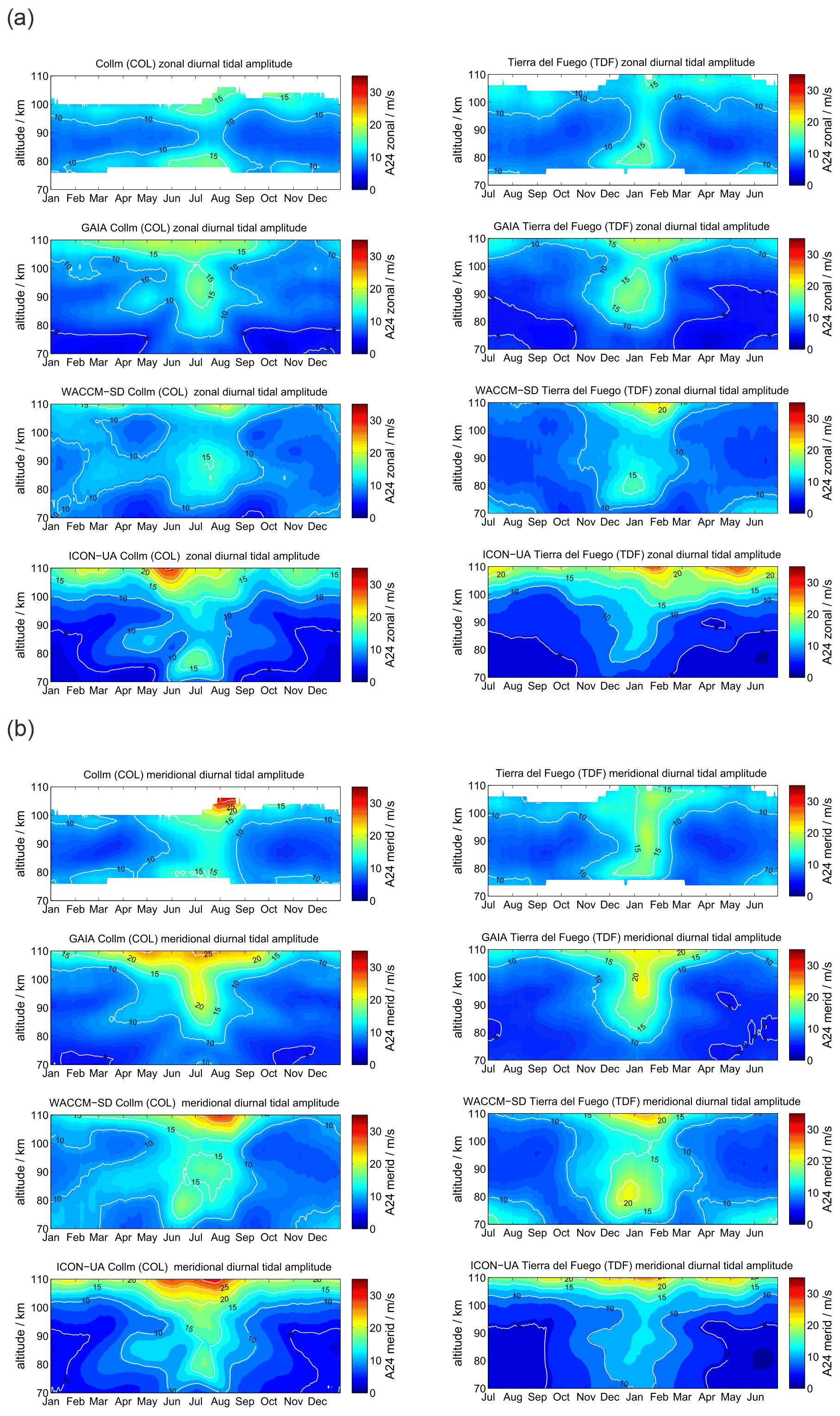
Diurnal tidal phases are presented in Fig. 11. Some of the features found at the polar latitudes are again visible at the midlatitudes. The seasonal characteristic of the diurnal tidal phases indicates some interhemispheric differences, which were already indicated for SOD and DAV. In the Northern Hemisphere the tidal phase shows a more pronounced biannual mode at altitudes above 84 km, whereas in the Southern Hemisphere an annual structure is more evident. All three models show dissimilarities in the seasonal vertical phase characteristic. Above 95 km GAIA and WACCM-X(SD) systematically deviate from the observations. UA-ICON exhibits an offset in the diurnal tidal phases compared to the observations as well as GAIA and WACCM-X(SD). In general, below 95 km, there is much better agreement between the observations and models.

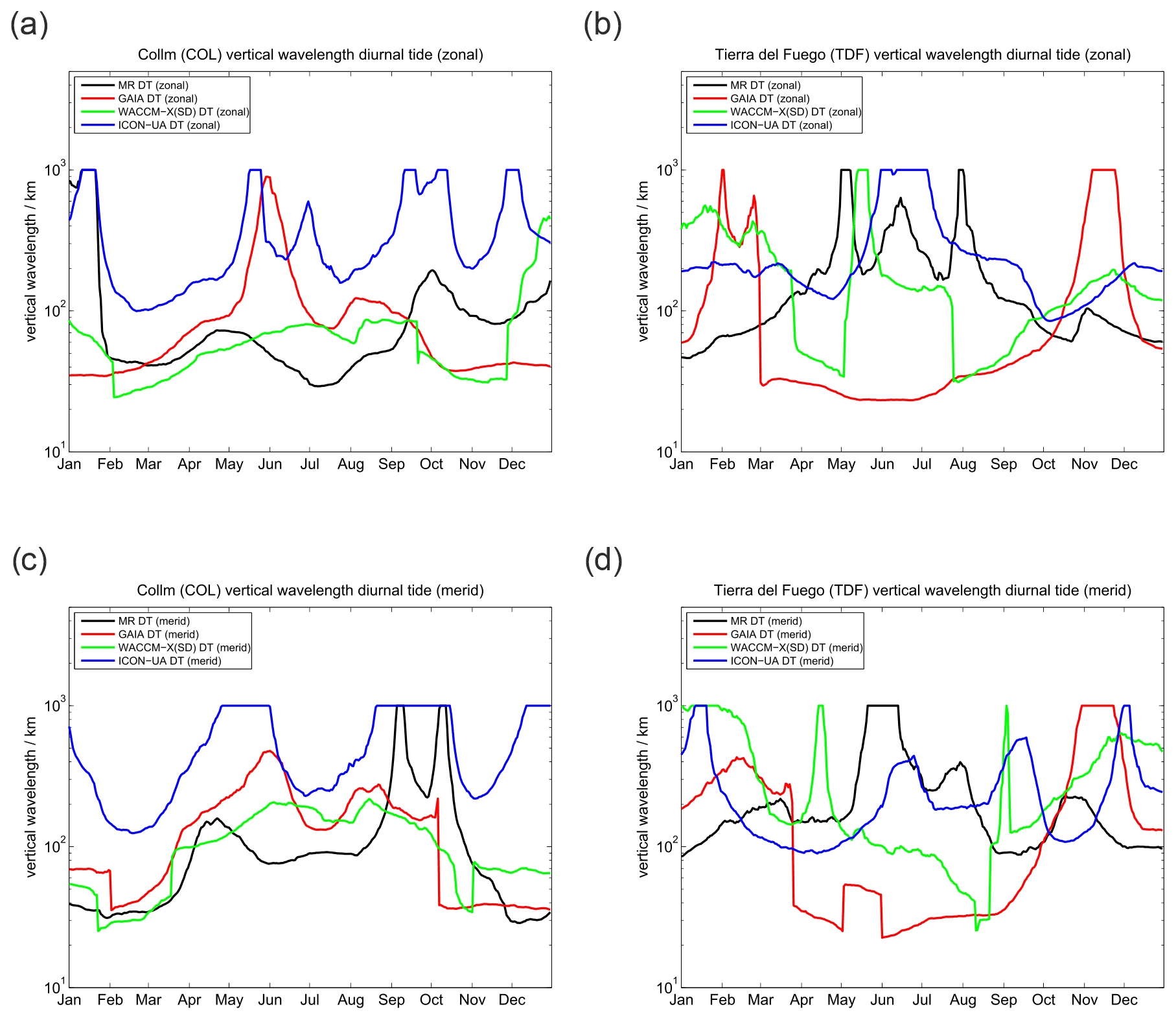
Figure 12 shows the vertical wavelength for the diurnal tide at the midlatitude locations above COL and TDF. All three models and the observations look dissimilar. Interestingly, an inter-model comparison also does not indicate substantial agreement for the vertical wavelengths between the different models. However, contrary to the polar latitudes UA-ICON now tends to overestimate the vertical wavelength a bit more compared to GAIA and WACCM-X(SD), which was opposite at polar latitudes.
We also estimated absolute amplitude differences for the diurnal tidal amplitudes for the COL and TDF MRs, which are shown in Appendix C2. During most times of the year the amplitudes are within ±5 m s−1, and only above 100 km can larger offsets of about 5–10 m s−1 be found. All three models tend to over estimate diurnal tidal amplitudes during the hemispheric summer months at altitudes between 80 and 95 km and to undervalue the diurnal tide during the winter months.
5.3 Semidiurnal tides
At midlatitudes the semidiurnal tide is the dominating atmospheric wave; it reaches amplitudes of about 50 m s−1 on average and occasionally up to 70 m s−1 above 90 km of altitude. The seasonal characteristic is presented in Fig. 13 and exhibits an inherent interhemispheric difference. The seasonal amplitude behavior at COL looks rather similar to that at SOD, but it reflects the much higher amplitudes during the winter months from November to February in the Northern Hemisphere. As expected (e.g., Jacobi, 2012), the zonal and meridional amplitudes are almost the same. Apparently, TDF in the Southern Hemisphere indicates a different seasonal amplitude characteristic. TDF still exhibits the largest amplitudes during the winter months from April to October, but with much weaker amplitudes compared to COL. Furthermore, at TDF the zonal component shows larger amplitudes than the meridional semidiurnal tide.
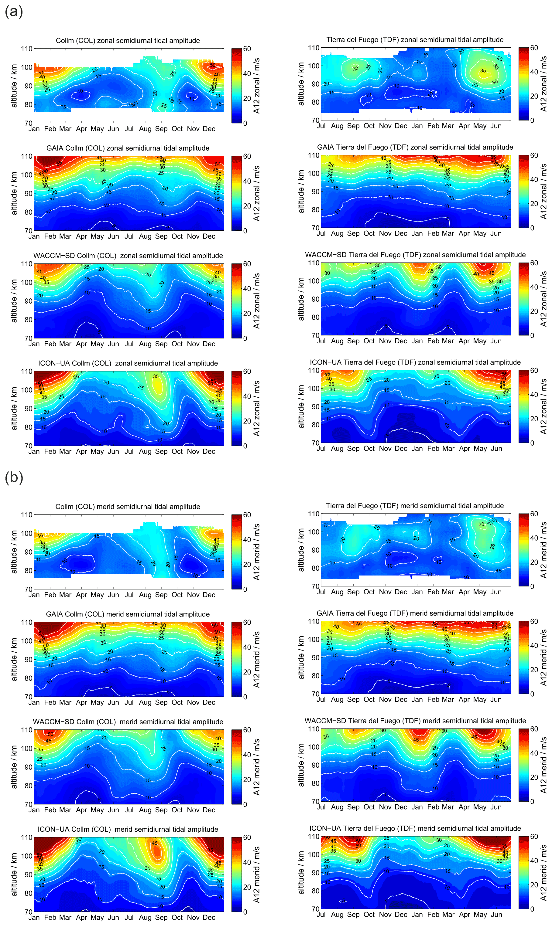
The GAIA model shows only a weak seasonality of the semidiurnal tidal amplitudes and even larger amplitudes above 100 km than the MR measurements. GAIA exhibits almost no interhemispheric differences of the tidal amplitudes. Only in the Northern Hemisphere does GAIA indicate a semidiurnal tidal enhancement for the winter months, as is found in the observations. WACCM-X(SD) and UA-ICON indicate a rather good representation of the semidiurnal tide in the Northern Hemisphere for the location of COL. The seasonality of the amplitudes is well-captured and exhibits remarkably good agreement compared with the observations. In the Southern Hemisphere the semidiurnal tides are less well-represented in WACCM-X(SD). The model shows a hemispheric summer tidal enhancement at altitudes above 90 km, which is missing in the observations. Furthermore, the amplitudes appear to be increased relative to the observations at TDF. For the hemispheric winter months above TDF, WACCM-X(SD) shows increased tidal amplitudes relative to the observations but captures the general hemispheric winter characteristic from May to July–August. Interestingly, UA-ICON indicates the best agreement with the observations for the seasonality of the semidiurnal tidal amplitudes in both hemispheres and even reproduces the interhemispheric differences quite well.
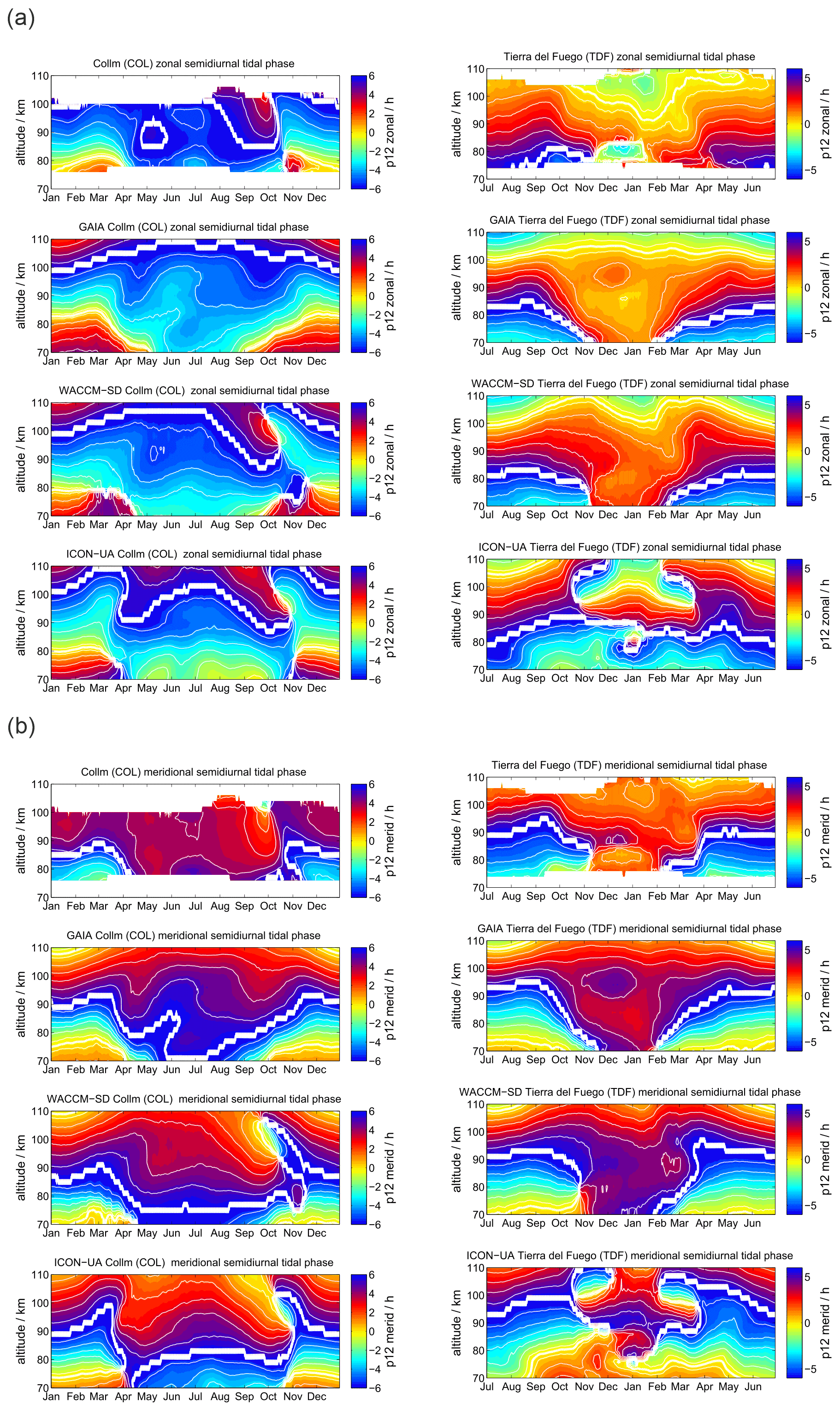
Semidiurnal tidal phases for the midlatitude conjugate comparison are shown in Fig. 14. The seasonal phase characteristic is rather similar compared to the polar latitudes. The measurements and the models indicate a significant interhemispheric difference that was already depicted in the amplitudes. In the Northern Hemisphere, we find a biannual seasonal phase characteristic in the observations that is well-reproduced in the WACCM-X(SD) and UA-ICON data. GAIA also shows reasonable agreement but does not reflect the quick phase change during the northern hemispheric fall transition in September–October. In the Southern Hemisphere the observations at TDF show a more smooth seasonal phase characteristic that appears to be only partially reproduced by the three models, which show distinguishable phase differences compared to the measurements.
Absolute semidiurnal tidal amplitude differences for COL and TDF are presented in Appendix D2. Semidiurnal tidal amplitudes appear to be systematically underestimated in the models by 5–10 m s−1 throughout the year at altitudes between 80 and 95 km. In the Southern Hemisphere above 95 km even larger differences emerge, but at these heights the models exceed the observed amplitudes by 15–20 m s−1 for both components.
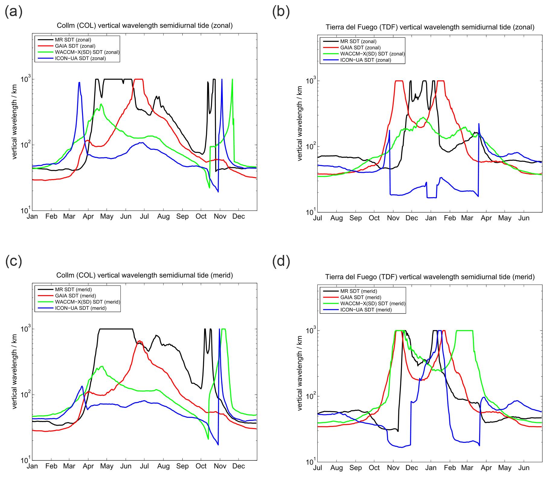
Vertical wavelengths are shown in Fig. 15. The observations indicate a clear seasonality of the vertical wavelengths, with much longer wavelengths during summer and during the fall and spring transitions. These long wavelengths seem to be associated with the seasonal characteristic of the westward zonal winds. Our observations indicate that during the hemispheric winter months vertical wavelengths of 40–90 km are common for the midlatitudes. As expected from the phases, GAIA shows the best agreement with the observations during the winter months and in the Southern Hemisphere. GAIA also shows the long wavelengths in the Northern Hemisphere summer. WACCM-X(SD) and UA-ICON tend to show reasonable agreement with the Northern Hemisphere and, in particular, show the rapid phase change during the fall transition. However, UA-ICON and WACCM-X(SD) also obtain similar wavelengths during the southern hemispheric winter months compared to the observations.
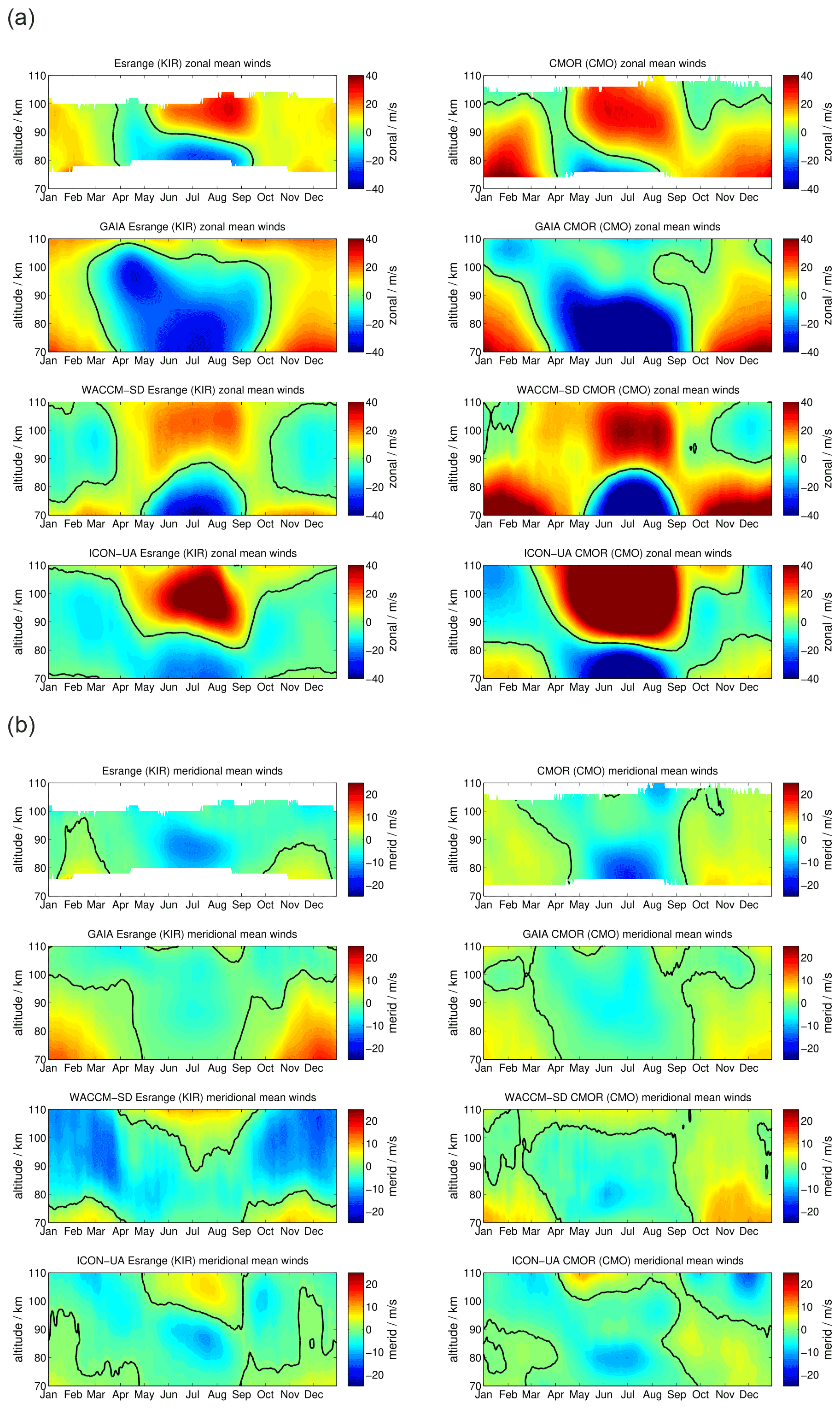
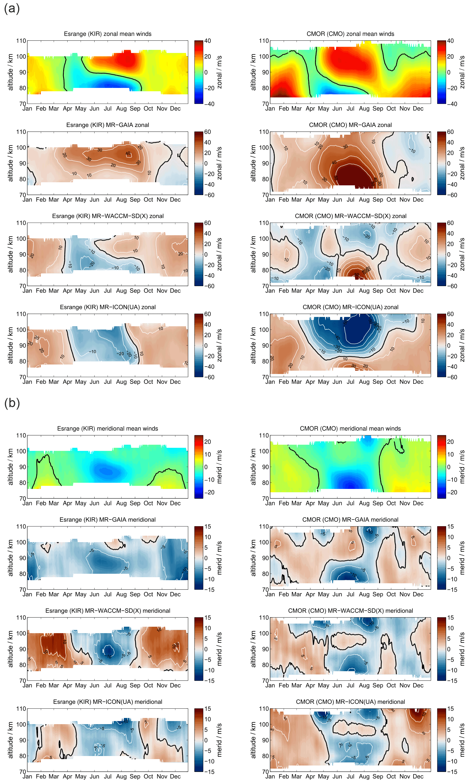
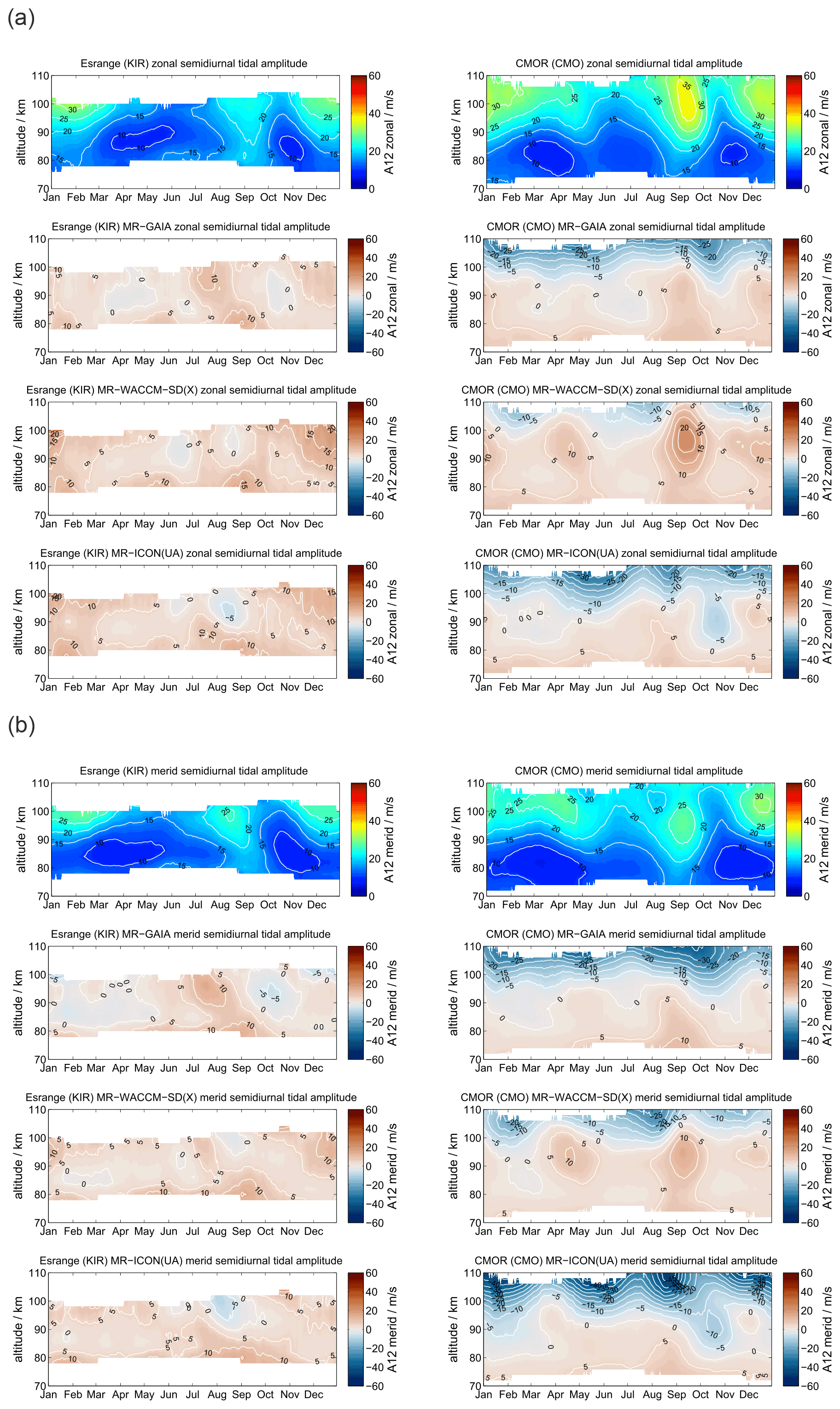
Finally, we investigate the KIR high-latitude meteor radar data and the CMOR observations in Canada, which is located at the lowest latitude used in this study. The KIR meteor radar is included as a sanity check for the robustness of the meteor radar observations as it is located in the proximity of SOD. In addition, these two stations provide a good comparison to show how the seasonal characteristic of mean winds as well as diurnal and semidiurnal tides change with latitude. The data are displayed in Figs. A1–A7.
The mean wind and tidal climatologies at SOD and KIR are almost identical and thus show similar agreement with GAIA, WACCM-X(SD), and UA-ICON. Comparing KIR and CMOR provides a more direct assessment of latitudinal differences. During the northern hemispheric winter CMOR observes an eastward zonal wind, which reaches higher magnitudes compared to KIR, but it also indicates a wind reversal above approximately 100 km to a weak westward wind. The summer wind reversal from westward to eastward occurs at an almost 5–8 km lower altitude relative to KIR. GAIA, WACCM-X(SD), and UA-ICON reproduce the increased strength of the eastward winds during the winter season but have difficulties reproducing the summer zonal wind reversal. GAIA underestimates the eastward acceleration above 90 km, whereas WACCM-X(SD) and UA-ICON overestimate the eastward zonal wind during the summer. Meridional winds exhibit a clear annual characteristic above CMOR. The general seasonal characteristic can also be found in GAIA, WACCM-X(SD), and UA-ICON.
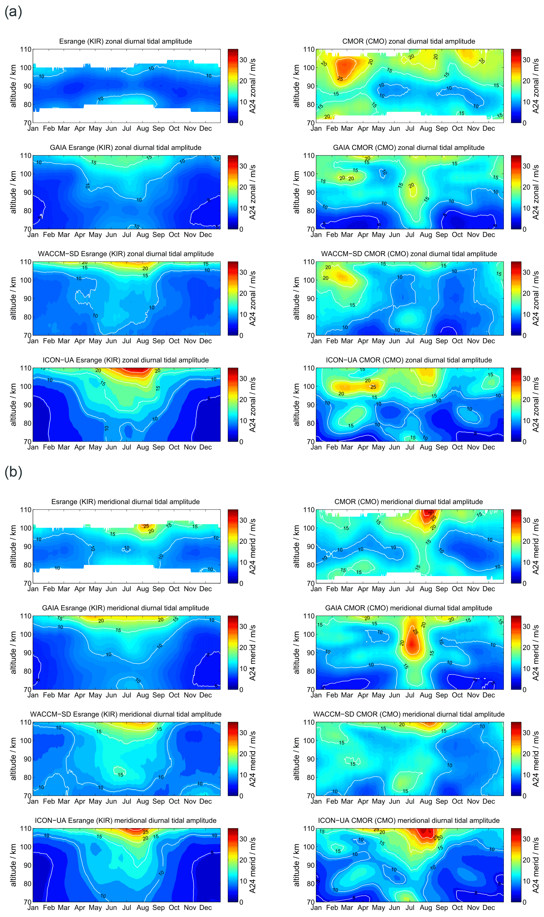
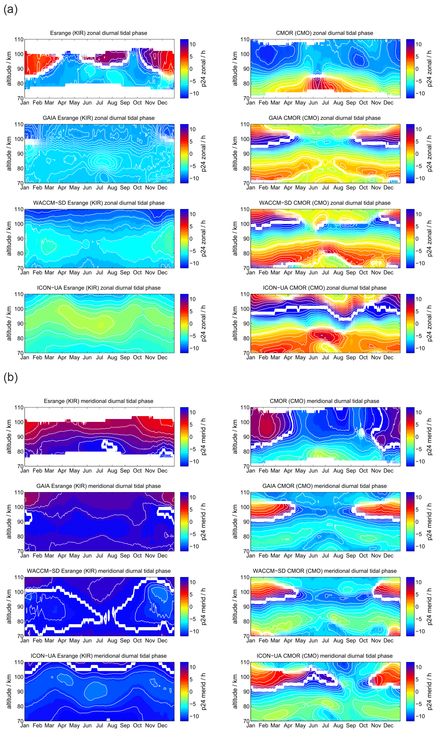
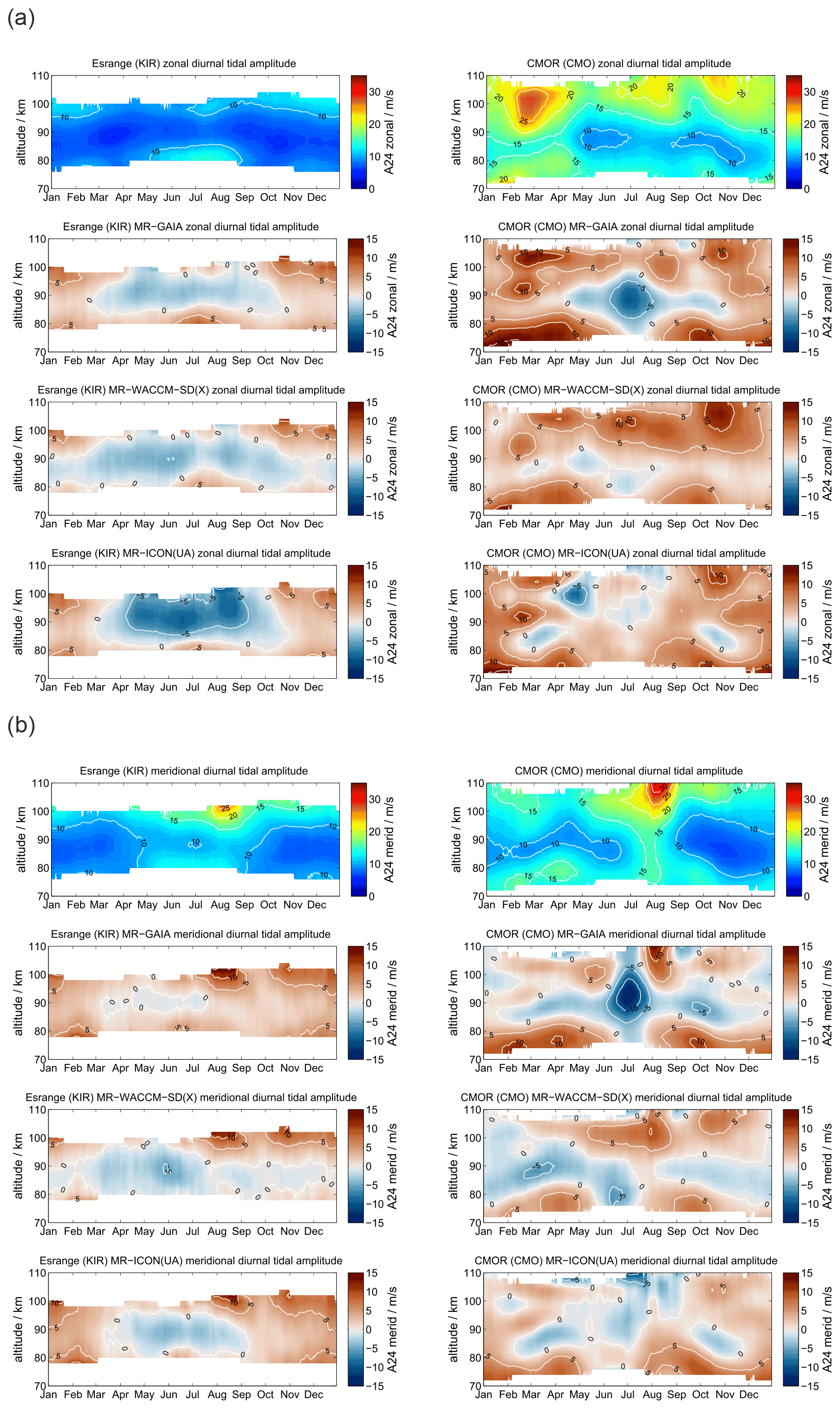
However, the diurnal tidal amplitudes and phases appear to be more difficult to be captured by the models for the CMOR location compared to the MR observations. WACCM-X(SD) and UA-ICON indicate better agreement of the diurnal tidal seasonal amplitude behavior relative to GAIA, but both models exhibit larger differences in the diurnal tidal phases above 90 km concerning the CMOR observation. This is also the case for the semidiurnal tidal amplitudes and phases. Both models indicate less good agreement with the observations of the seasonal characteristic of the semidiurnal tidal amplitude. However, the phases of the semidiurnal tide indicate better agreement with the observations. In particular, WACCM-X(SD) captures the seasonal variability during the fall transition remarkably well. UA-ICON tends to show larger dissimilarities compared to the observations and WACCM-X(SD) for the CMOR locations.
Absolute differences for mean winds as well as diurnal and semidiurnal tidal amplitudes for CMO and KIR are presented in Appendices B3, C3, and D3. The MR KIR reflects the same absolute differences for GAIA, WACCM-X(SD), and UA-ICON that we found for the SOD location. However, at the midlatitude station CMO the models exhibit differences of ±50 m s−1 for the zonal wind component during the hemispheric summer, which is mostly due to differences in the altitude of the summer wind reversal and substantial differences in the strength of the eastward summer jet above 90 km. Meridional winds indicate differences of ±5 m s−1 and only occasionally offsets of more than 10 m s−1.
The mean circulation at the MLT is substantially controlled by tides and gravity waves, carrying energy and momentum from their source regions to the altitude of their dissipation (e.g., Lindzen, 1981, and references therein). Gravity wave dissipation drives the hemispheric summer mesopause temperatures up to 100 K away from the radiative equilibrium (McLandress et al., 2006; Becker, 2012; Smith, 2012; Sato et al., 2018). However, GCMs often do not have the spatial and temporal resolution to resolve GWs and thus depend on GW parameterizations of the different primary GW sources such as orography (mountain waves), frontal systems, jet stream imbalances, deep convection, and shear instabilities (Fritts and Alexander, 2003; Plougonven and Zhang, 2014, also see for a review). Recently, there were studies suggesting that non-primary GWs also contribute to the momentum budget at the MLT (Vadas and Becker, 2018; Vadas et al., 2018; Becker and Vadas, 2018; Sato et al., 2018), resulting in an even more complex vertical coupling and posing new challenges not yet considered in available GW parameterizations.
GAIA and WACCM-X(SD) both incorporate similar GW parameterizations for orographic and non-orographic primary GWs based on McFarlane (1987) and Lindzen (1981). Although the applied schemes are supposed to be comparable, the resulting forcing is rather dissimilar concerning the magnitude of the parameterized GW drag. UA-ICON uses different GW parameterizations (Giorgetta et al., 2018; Hines, 1997; Lott, 1999), which are, however, structurally similar with typical simplifying assumptions like pure vertical and instantaneous propagation of GWs. Pedatella et al. (2014) estimated the mean zonal GW drag from GAIA and WACCM-X by applying the relation shown in H.-L. Liu et al. (2009). The net zonal mean GW drag was more than twice as large in WACCM-X(SD) compared to GAIA at middle and polar latitudes from the stratosphere up to the mesosphere. The comparison also indicated differences in the vertical structure of where the GW drag accelerates or decelerates the mean zonal wind and hence explains why the mean wind structures are different between GAIA and WACCM-X(SD). The GW parameterization of UA-ICON is similar to the HAMMONIA model, which has been shown by Pedatella et al. (2014) to produce mesospheric GW drag smaller than WACCM-X but larger than GAIA. Apparently, the parameterization in WACCM-X(SD) seems to be more suitable to reproduce the hemispheric summer mesopause zonal wind reversal, whereas the GAIA GW parameterization is more adequate for hemispheric winter conditions.
In the past, GCMs were often validated and cross-compared to other global data sets such as satellite observations using typical winter or summer conditions and comparing zonal means as vertical-latitude cross sections (McLandress et al., 1996; McLandress, 1997; Du et al., 2007; H.-L. Liu et al., 2009; Smith, 2012; Liu et al., 2013; Pedatella et al., 2014). Ground-based observations open the possibility to perform a better climatological comparison, but only for a given location. McCormack et al. (2017) conducted a cross-validation between the meteorological analysis with NAVGEM-HA and globally distributed MR wind measurements using altitude vs. time plots to access the temporal and short-term variability of mean winds and tides for two winter seasons. Later, Stober et al. (2020a) performed a cross-comparison of the seasonal climatology for three MR stations and a more detailed verification of the tidal variability of the tidal amplitude and phase behavior using NAVGEM-HA and MRs. These comparisons revealed remarkable agreement between the observations and the meteorological analysis on interday to seasonal timescales for mean winds as well as for atmospheric tides, providing confidence in both data sets to capture realistic atmospheric dynamics in the MLT.
In this study, we present the first systematic investigation of interhemispheric differences of mean winds and atmospheric tides at conjugate latitudes from observations and comprehensive models by applying a unified diagnostic. Although the results are in line with other studies using MR observations to evaluate mean winds and tides in the MLT, they reveal in more detail the latitudinal differences between the two hemispheres and present a more systematic evaluation of state-of-the-art models at the MLT. Pancheva et al. (2020) compared MR observations from Svalbard and Tromsø to WACCM-X and CMAM-DAS and found similar agreements and deviations concerning the seasonality of mean winds and tides. In particular, their results obtained from Tromsø are comparable to SOD and KIR. Sato et al. (2018) compared GAIA to Microwave Limb Sounder (MLS) temperatures and geostrophic winds for January conditions and found very good agreement from 12 km of altitude up to 80 km for the Southern Hemisphere, and up to 97 km for the Northern Hemisphere. This comparison also indicated a summer zonal wind reversal for the southern latitudes in GAIA that is too weak and high up, in contrast to Yasui et al. (2018), stating that the missing wind reversal may be due to the limitation of the representation of the parameterized gravity waves in the model. Some of the differences between GAIA, WACCM-X(SD), and the MR observations have their origin further down in the atmosphere. Both models are nudged to the reanalysis data. GAIA is nudged to the JRA-25 and from 2015 on to JRA-55 reanalysis data (Kobayashi et al., 2015) up to 30 km, whereas WACCM-X(SD) is driven by MERRA (Rienecker et al., 2011) up to 50 km. Harada et al. (2016) performed a cross-comparison among various reanalysis data sets to investigate potential differences and found that JRA-25, JRA-55, and MERRA already showed some differences in storm tracks and mean winds and temperatures. In particular, at the upper stratosphere the reanalysis data sets and observation from MLS indicated some differences among each other. Due to the nudging of GAIA and WACCM-X(SD), these differences also enter the model fields and partly explain differences among the models as well as concerning the MR observations. The nudging height may also play some role since the systematic differences have been found in the upper stratosphere (Sakazaki et al., 2018).
Furthermore, the reanalysis data used for the nudging of GAIA and WACCM-X(SD) seem to be less relevant for the representation of the diurnal and semidiurnal migrating tide climatologies. It is also worth considering that reanalysis data depend on the data assimilation cadence. MERRA2 updates the fields every 6 h using a 3D-Var scheme, although a 3-hourly output is provided (Gelaro et al., 2017), which limits a realistic forcing for the semidiurnal tide concerning the amplitude and phase. Ortland (2017) estimated the tidal forcing for the DW1 and SW2 due to absorption of solar radiation from ozone and water vapor. Therein it was found that the tidal correspondence between the Tide Mean Assimilation Model (TMAT) and observations at the MLT strongly depends on the forcing at the troposphere and stratosphere for both migrating tides. Thus, differences in the tides between the models are most likely the result of different implementations of the radiative transfer and distribution of tropospheric–stratospheric water vapor and ozone causing differences in the radiative forcing. This is further supported by the free-running UA-ICON, which shows very good agreement with the tides produced in WACCM-X(SD) but is not driven by any reanalysis data.
Another aspect worth discussing involves the tidal phases. Apparently, WACCM-X(SD), UA-ICON, and GAIA reach fairly good agreement with the semidiurnal tidal phases at middle and polar latitudes, capturing many of the seasonal characteristics that are found in the MR observations. It is also obvious that GAIA tends to agree better in the Southern Hemisphere and WACCM-X(SD) performs a bit better in the Northern Hemisphere. Only the diurnal tidal phases at polar latitudes are dissimilar in both models compared to the MR observations. The vertical wavelength of the diurnal tides in GAIA and WACCM-X(SD) suggest almost evanescent diurnal tidal modes, whereas the observations indicate much shorter wavelengths and a vertically propagating diurnal tide. Both models reduce the longitudinal grid resolution closer to the pole to avoid the singularity. This seems to favor a damped vertical propagation of the diurnal tide but has to be investigated in more detail.
Non-migrating tides are also worth discussing. In fact, our MR observations are local, and thus the observed diurnal and semidiurnal tides are a superposition of the migrating and non-migrating tidal modes. At the lower latitudes, the generation of non-migrating tides is well-understood due to the latent heat release in the tropics (Hagan and Forbes, 2002, 2003; Oberheide et al., 2011). At middle and polar latitudes non-migrating tides can be generated by various processes such as latent heat release, nonlinear interactions with stationary planetary waves (Yamashita et al., 2002; Smith et al., 2007; Murphy et al., 2009; Miyoshi et al., 2017) and other tidal modes, variations in the mean background wind and temperature field, and gravity wave breaking or dissipation regions (Fritts et al., 2006). Furthermore, there were some studies investigating SSW as a potential cause to excite the westward-propagating semidiurnal tides with wavenumbers 1 and 3 (Du et al., 2007; Liu et al., 2010b; Stober et al., 2020b).
There are only a few studies investigating the climatology of non-migrating tides available using ground-based networks. Murphy et al. (2006) presented a climatology of the diurnal and semidiurnal tides for the Southern Hemisphere combining several radars located in Antarctica. Their results indicate that the amplitudes of the non-migrating components are between 1 and 5 m s−1 and occasionally reach up to 10 m s−1. However, this study also confirmed that the migrating component is the dominating tide most times of the year, which was also found in Baumgarten and Stober (2019) during a campaign in the Northern Hemisphere. Recently, there were some studies in the Northern Hemisphere based on SuperDARN observations to derive climatologies of the migrating (van Caspel et al., 2020) and non-migrating tides (Hibbins et al., 2019). These studies revealed amplitudes of about 5 m s−1 throughout the year for the non-migrating components and amplitudes of about 15–20 m s−1 for the migrating tidal components at high polar latitudes. Considering the various non-migrating tidal generation mechanism it is obvious that there is only a weak coherence between the years due to phase variability of their source processes (e.g., SSWs occur at different dates from year to year in the Northern Hemisphere). Hence, the obtained tidal climatological comparison presented here is dominated by the migrating tidal components. The comparison of the free-running UA-ICON model with the nudged GAIA and WACCM-X(SD) indicates that the climatology of mean winds and tides at the MLT is driven by the model physics and does not strongly depend on the nudging at the troposphere–stratosphere. Apparently UA-ICON and WACCM-X(SD) employ GW parameterizations that yield a similar climatological wind at the MLT, although the detailed implementation is different. Furthermore, the good agreement of the tidal amplitude and phases between WACCM-X(SD) and UA-ICON suggests that the seasonal characteristics and the resultant tidal climatologies are also less dependent on the nudging. Recently, Dempsey et al. (2021) performed a cross-comparison of mean winds and tides in the Southern Hemisphere using the meteor radar at Rothera and WACCM as well as the Extended Canadian Middle Atmosphere Model (eCMAM). They postulated that non-primary waves play a role for the MLT winds. Theoretical studies with the Kuehlungsborn Mechanistic Circulation Model (KMCM) showed that secondary or non-primary wave generation provides an essential contribution to the MLT wind forcing above GW hot spots such as the southern Andes and the Antarctic Peninsula (Becker and Vadas, 2018; Vadas and Becker, 2018). The first observational evidence was obtained at McMurdo through an investigation of lidar observations (Vadas et al., 2018). More recently a detailed study of the MLT dynamics for the year 2019 using six meteor radars from Tierra del Fuego, South Georgia, Rothera, King Sejong Station, Davis, and McMurdo indicated a strong impact of non-primary waves above the Andes and Antarctic Peninsula on the daily mean zonal and meridional winds and momentum fluxes (Stober et al., 2021b). Including non-primary waves in the GW parameterizations for the hemispheric winter could add eastward momentum to the MLT, which is apparently too weak in WACCM-X(SD) and UA-ICON. The strong winter stratospheric eastward polar vortex efficiently removes all eastward GWs by critical level filtering, and thus only westward GWs propagate to the mesosphere and can deposit their momentum, resulting in an westward forcing and westward mean winds. Considering non-primary waves in the parameterization could essentially balance the total forcing at the MLT and may help to bring the mean winds into better agreement with the observations.
In this study we compared GAIA, UA-ICON, and WACCM-X(SD) predictions with local meteor radar observations by applying a unified diagnostic to decompose the wind field into mean winds as well as diurnal and semidiurnal tidal amplitudes and phases in the MLT. Therefore, we present observations from six meteor radars and derived climatologies from the continuous observations for the abovementioned meteorological parameters, which are cross-compared to nudged model simulations from GAIA and WACCM-X(SD) for the same periods that the measurements are available from each radar. In addition, a 21-year UA-ICON free-running GCM run was employed for comparison.
Although all models utilize similar gravity wave parameterization schemes but different implementations, the zonal and meridional winds exhibit seasonal and interhemispheric differences between GAIA, WACCM-X(SD), UA-ICON, and the MR observations. It is obvious that GAIA shows better agreement of mean winds during the winter season in both hemispheres compared to the meteor radar, whereas WACCM-X(SD) and UA-ICON indicate better agreement of the zonal wind reversal from westward to eastward in both hemispheres with the observations. However, one has to note that GAIA seems to produce a hemispheric summer zonal wind reversal that is too weak and too high up. WACCM-X(SD) and UA-ICON tend to show westward winds during the winter season, pointing towards too much westward wave drag at these altitudes. Furthermore, meridional winds appear to be in remarkable agreement between GAIA and the MR observations at middle and polar latitudes, while WACCM-X(SD) and UA-ICON indicate more dissimilarities in the meridional winds relative to the MR observations. UA-ICON, as a free-running model, nevertheless shows a remarkably good representation of MLT wind fields compared to the two nudged models.
The ASF decomposition of the time series from the models and the meteor radar observations ensures a harmonized tidal comparison of the amplitude and phases. Atmospheric tides provide an essential source of variability for the coupling of the middle atmosphere to the ionosphere. Daily tidal amplitudes and phase are obtained from the ASF and vector-averaged, which reduces the contamination of the amplitude and phase due to the tidal intermittency caused by nonlinear wave–wave interactions, changes in the mean winds, or source variabilities. There is good agreement of the GCMs for the diurnal tide amplitude and phase for the latitudes investigated herein. Diurnal tides indicate only weak interhemispheric differences and reach the largest amplitudes above 95–100 km during the hemispheric summer months. The seasonality of the diurnal tidal amplitudes is well-reproduced by GAIA, UA-ICON, and WACCM-X(SD). However, diurnal tidal phases show some differences between the observations and the GCMs. GAIA, UA-ICON, and WACCM-X(SD) tend to exhibit much longer vertical wavelengths compared to the MR measurements.
Semidiurnal tides are the dominating tidal mode at middle and high latitudes through the course of the year and at MLT altitudes. Some of the main results of this comparison are the distinct differences of this tide between the two hemispheres. It appears that for conjugate latitudes the semidiurnal tide reaches higher amplitudes in the Northern Hemisphere at middle and polar latitudes. In particular, the amplitude enhancement and phase variability in September in the Northern Hemisphere are not found at the southern latitudes during the transition from the hemispheric summer to the winter circulation. More detailed investigations are required to distinguish potential reasons, which are likely caused by a complex chain of interactions due to the differences in the land–sea distribution, GW sources, and planetary waves between the two hemispheres that alter the polar vortices and thus the ozone transport into the polar cap, which again provides a feedback on the excitation of tides. GAIA, UA-ICON, and WACCM-X(SD) indicate reasonable agreement of the semidiurnal tidal amplitude and phase. There is a tendency for WACCM-X(SD) and UA-ICON to have better agreement with the MR observations in the Northern Hemisphere, whereas GAIA seems to agree better in the Southern Hemisphere. However, all GCMs have a tendency to overestimate the summer hemisphere semidiurnal tidal amplitudes above 100 km.
The climatological comparisons of mean winds and diurnal and semidiurnal tides underline the value of continuous observations in the MLT to evaluate and assess GCMs. GAIA, WACCM-X(SD), and UA-ICON are state-of-the-art models, coupling the middle atmosphere with the upper atmosphere to study the forcing from below of the thermosphere–ionosphere system and a potential feedback to the middle atmosphere. Therefore, we assessed the climatological state of the mean winds and the tidal activity at the MLT. We identified systematic dissimilarities in the mean zonal and meridional winds and in the seasonal characteristic of tidal amplitudes and phases. However, there was remarkable agreement in both hemispheres of the semidiurnal tide between the observations and the free-running UA-ICON, which further underlines the fact that the climatological behavior at the MLT seems not to be driven and/or improved by the nudging of GCMs to reanalysis data for the semidiurnal tide.


The dataset used for this study is from the Ground-to-topside model of Atmosphere and Ionosphere for Aeronomy (GAIA) project carried out by the National Institute of Information and Communications Technology (NICT), Kyushu Universty, and Seikei University. The 3-hourly SD/WACCM-X v2.1 simulation output for 1980–2017 is archived on NCAR's CDG repository and can be accessed online (https://doi.org/10.26024/5b58-nc53, NOAA National Geophysical Data Center, 2009). The MR radar data can be obtained upon request from the instrument PIs.
The conceptual idea for the paper was developed by GS, DP, CJ, and HL. The data analysis and data reduction were performed by AlKu and DP. HL supported the data analysis and interpretation of GAIA and contributed to the discussion. HLL supported the interpretation of the WACCM-X(SD) results and the overall discussion. HS provided the UA-ICON data and helped with the interpretation of the results. KB provided an essential contribution to developing the ASF method. All authors contributed to the editing and writing of the paper. AlKo and ML provided SGO meteor radar data. EB and JK contributed the Esrange meteor radar observations. DJ shared the TDF meteor radar measurements, and DM supported this work by providing DAV data. PB provided the CMOR radar data.
The authors declare that they have no conflict of interest.
Publisher's note: Copernicus Publications remains neutral with regard to jurisdictional claims in published maps and institutional affiliations.
Gunter Stober is a member of the Oeschger Center for Climate Change Research (OCCR). The Esrange meteor radar operation, maintenance and data collection is provided by Esrange Space Center of Swedish Space Corporation. We thank Hidekatsu Jin for providing the long-term GAIA simulation data.
Ales Kuchar and Christoph Jacobi acknowledge support by the Deutsche Forschungsgemeinschaft through grant no. JA 836/43-1. Huixin Liu acknowledges support by JSPS KAKENHI grant nos. 18H01270, 18H04446, 17KK0095, and JRPs-LEAD with DFG. Han-Li Liu's effort is partially supported by NASA (grant nos. 80NSSC20K1323, 80NSSC20K0601, 80NSSC20K0633) and the NSF (grant no. OPP 1443726). The National Center for Atmospheric Research is a major facility sponsored by the National Science Foundation under cooperative agreement no. 1852977. Operation of the Davis meteor radar is supported through Australian Antarctic Science projects 2668, 4025, and 4445. Diego Janches was supported by the NASA Heliophysics ISFM program. TDF's operation is supported by NASA NESC assessment TI-17-01204. This work was supported in part by the NASA Meteoroid Environment Office under cooperative agreement no. 80NSSC18M0046. PGB's operation was supported in part by the NASA Meteoroid Environment Office under cooperative agreement no. 80NSSC21M0073. PGB also acknowledges funding support from the Natural Sciences and Engineering Research Council of Canada (RGPIN-2016-04433) and the Canada Research Chairs program (grant no. 950-231930).
This paper was edited by Bernd Funke and reviewed by Andreas Dörnbrack and one anonymous referee.
Amante, C. and Eakins, B.: ETOPO1 1 Arc-Minute Global Relief Model: Procedures, Data Sources and Analysis, NOAA Technical Memorandum NESDIS NGDC-24, National Geophysical Data Center, NOAA, https://doi.org/10.7289/V5C8276M, 2009. a
Andrews, D. G., Holton, J. R., and Leovy, C. B.: Middle Atmosphere Dynamics, Academic Press, San Diego, CA, 1987. a
Baumgarten, K. and Stober, G.: On the evaluation of the phase relation between temperature and wind tides based on ground-based measurements and reanalysis data in the middle atmosphere, Ann. Geophys., 37, 581–602, https://doi.org/10.5194/angeo-37-581-2019, 2019. a, b, c, d
Becker, E.: Dynamical Control of the Middle Atmosphere, Space Sci. Rev., 168, 283–314, https://doi.org/10.1007/s11214-011-9841-5, 2012. a, b
Becker, E. and Vadas, S. L.: Secondary Gravity Waves in the Winter Mesosphere: Results From a High-Resolution Global Circulation Model, J. Geophys. Res.-Atmos., 123, 2605–2627, https://doi.org/10.1002/2017JD027460, 2018. a, b, c
Borchert, S., Zhou, G., Baldauf, M., Schmidt, H., Zängl, G., and Reinert, D.: The upper-atmosphere extension of the ICON general circulation model (version: ua-icon-1.0), Geosci. Model Dev., 12, 3541–3569, https://doi.org/10.5194/gmd-12-3541-2019, 2019. a, b, c, d
Conte, J. F., Chau, J. L., Stober, G., Pedatella, N., Maute, A., Hoffmann, P., Janches, D., Fritts, D., and Murphy, D. J.: Climatology of semidiurnal lunar and solar tides at middle and high latitudes: Interhemispheric comparison, J. Geophys. Res.-Space, 122, 7750–7760, https://doi.org/10.1002/2017JA024396, 2017. a
Crueger, T., Giorgetta, M. A., Brokopf, R., Esch, M., Fiedler, S., Hohenegger, C., Kornblueh, L., Mauritsen, T., Nam, C., Naumann, A. K., Peters, K., Rast, S., Roeckner, E., Sakradzija, M., Schmidt, H., Vial, J., Vogel, R., and Stevens, B.: ICON-A, The atmosphere component of the ICON Earth system model: II. Model evaluation, J. Adv. Model. Earth Sy., 10, 1638–1662, https://doi.org/10.1029/2017MS001233, 2018. a
de Wit, R. J., Janches, D., Fritts, D. C., Stockwell, R. G., and Coy, L.: Unexpected climatological behavior of MLT gravity wave momentum flux in the lee of the Southern Andes hot spot, Geophys. Res. Lett., 44, 1182–1191, https://doi.org/10.1002/2016GL072311, 2017. a
Dempsey, S. M., Hindley, N. P., Moffat-Griffin, T., Wright, C. J., Smith, A. K., Du, J., and Mitchell, N. J.: Winds and tides of the Antarctic mesosphere and lower thermosphere: One year of meteor-radar observations over Rothera (68∘ S, 68∘ W) and comparisons with WACCM and eCMAM, J. Atmos. Sol.-Terr. Phy., 212, 105510, https://doi.org/10.1016/j.jastp.2020.105510, 2021. a
Du, J., Ward, W., Oberheide, J., Nakamura, T., and Tsuda, T.: Semidiurnal tides from the extended Canadian Middle Atmosphere Model (CMAM) and comparisons with TIMED Doppler interferometer (TIDI) and meteor radar observations, J. Atmos. Sol.-Terr. Phy., 69, 2159–2202, https://doi.org/10.1016/j.jastp.2007.07.014, 2007. a, b
Eckermann, S. D., Ma, J., Hoppel, K. W., Kuhl, D. D., Allen, D. R., Doyle, J. A., Viner, K. C., Ruston, B. C., Baker, N. L., Swadley, S. D., Whitcomb, T. R., Reynolds, C. A., Xu, L., Kaifler, N., Kaifler, B., Reid, I. M., Murphy, D. J., and Love, P. T.: High-Altitude (0-100 km) Global Atmospheric Reanalysis System: Description and Application to the 2014 Austral Winter of the Deep Propagating Gravity Wave Experiment (DEEPWAVE), Mon. Weather Rev., 146, 2639–2666, https://doi.org/10.1175/MWR-D-17-0386.1, 2018. a, b
Emmert, J.: Thermospheric mass density: A review, Adv. Space Res., 56, 773–824, https://doi.org/10.1016/j.asr.2015.05.038, 2015. a
Fritts, D. and Alexander, M. J.: Gravity wave dynamics and effects in the middle atmosphere, Rev. Geophys., 41, 1–64, https://doi.org/10.1029/2001RG000106, 2003. a
Fritts, D. C., Vadas, S. L., Wan, K., and Werne, J. A.: Mean and variable forcing of the middle atmosphere by gravity waves, J. Atmos. Sol.-Terr. Phy., 68, 247–265, https://doi.org/10.1016/j.jastp.2005.04.010, 2006. a
Garcia, R. R., Smith, A. K., Kinnison, D. E., Cámara, A. d. l., and Murphy, D. J.: Modification of the Gravity Wave Parameterization in the Whole Atmosphere Community Climate Model: Motivation and Results, J. Atmos. Sci., 74, 275–291, https://doi.org/10.1175/JAS-D-16-0104.1, 2017. a
Gasperini, F., Liu, H., and McInerney, J.: Preliminary Evidence of Madden-Julian Oscillation Effects on Ultrafast Tropical Waves in the Thermosphere, J. Geophys. Res.-Space, 125, e2019JA027649, https://doi.org/10.1029/2019JA027649, 2020. a
Gelaro, R., McCarty, W., Suárez, M. J., Todling, R., Molod, A., Takacs, L., Randles, C. A., Darmenov, A., Bosilovich, M. G., Reichle, R., Wargan, K., Coy, L., Cullather, R., Draper, C., Akella, S., Buchard, V., Conaty, A., da Silva, A. M., Gu, W., Kim, G.-K., Koster, R., Lucchesi, R., Merkova, D., Nielsen, J. E., Partyka, G., Pawson, S., Putman, W., Rienecker, M., Schubert, S. D., Sienkiewicz, M., and Zhao, B.: The Modern-Era Retrospective Analysis for Research and Applications, Version 2 (MERRA-2), J. Climate, 30, 5419–5454, https://doi.org/10.1175/JCLI-D-16-0758.1, 2017. a
Giorgetta, M. A., Brokopf, R., Crueger, T., Esch, M., Fiedler, S., Helmert, J., Hohenegger, C., Kornblueh, L., Köhler, M., Manzini, E., Mauritsen, T., Nam, C., Raddatz, T., Rast, S., Reinert, D., Sakradzija, M., Schmidt, H., Schneck, R., Schnur, R., Silvers, L., Wan, H., Zängl, G., and Stevens, B.: ICON-A, the atmosphere component of the ICON Earth System Model: I. Model description, J. Adv. Model. Earth Sy., 10, 1613–1637, https://doi.org/10.1029/2017MS001242, 2018. a, b, c, d
Hagan, M. E. and Forbes, J. M.: Migrating and nonmigrating diurnal tides in the middle and upper atmosphere excited by tropospheric latent heat release, J. Geophys. Res.-Atmos., 107, ACL 6-1–ACL 6-15, https://doi.org/10.1029/2001JD001236, 2002. a
Hagan, M. E. and Forbes, J. M.: Migrating and nonmigrating semidiurnal tides in the upper atmosphere excited by tropospheric latent heat release, J. Geophys. Res., 108, 1062, https://doi.org/10.1029/2002JA009466, 2003. a
Harada, Y., Kamahori, H., Kobayashi, C., Endo, H., Kobayashi, S., Ota, Y., Onoda, H., Onogi, K., Kengo, M., and Takahashi, K.: The JRA-55 Reanalysis: Representation of Atmospheric Circulation and Climate Variability, J. Meteorol. Soc. Jpn. Ser. II, 94, 269–302, https://doi.org/10.2151/jmsj.2016-015, 2016. a
Heelis, R. A., Lowell, J. K., and Spiro, R. W.: A model of the high-latitude ionospheric convection pattern, J. Geophys. Res.-Space, 87, 6339–6345, https://doi.org/10.1029/JA087iA08p06339, 1982. a
Hibbins, R. E., Espy, P. J., Orsolini, Y. J., Limpasuvan, V., and Barnes, R. J.: SuperDARN Observations of Semidiurnal Tidal Variability in the MLT and the Response to Sudden Stratospheric Warming Events, J. Geophys. Res.-Atmos., 124, 4862–4872, https://doi.org/10.1029/2018JD030157, 2019. a
Hines, C. O.: Doppler-spread parameterization of gravity-wave momentum deposition in the middle atmosphere. Part 1: Basic formulation, J. Atmos. Sol.-Terr. Phy., 59, 371–386, 1997. a, b
Hocking, W., Fuller, B., and Vandepeer, B.: Real-time determination of meteor-related parameters utilizing modern digital technology, J. Atmos. Sol.-Terr. Phy., 63, 155–169, https://doi.org/10.1016/S1364-6826(00)00138-3, 2001. a, b
Holdsworth, D. A., Reid, I. M., and Cervera, M. A.: Buckland Park all-sky interferometric meteor radar, Radio Science, 39, rS5009, https://doi.org/10.1029/2003RS003014, 2004. a, b
Hurrell, J. W., Holland, M. M., Gent, P. R., Ghan, S., Kay, J. E., Kushner, P. J., Lamarque, J. F., Large, W. G., Lawrence, D., Lindsay, K., Lipscomb, W. H., Long, M. C., Mahowald, N., Marsh, D. R., Neale, R. B., Rasch, P., Vavrus, S., Vertenstein, M., Bader, D., Collins, W. D., Hack, J. J., Kiehl, J., and Marshall, S.: The Community Earth System Model: A Framework for Collaborative Research, B. Am. Meteorol. Soc., 94, 1339–1360, https://doi.org/10.1175/BAMS-D-12-00121.1, 2013. a
Iimura, H., Fritts, D. C., Tsutsumi, M., Nakamura, T., Hoffmann, P., and Singer, W.: Long-term observations of the wind field in the Antarctic and Arctic mesosphere and lower-thermosphere at conjugate latitudes, J. Geophys. Res., 116, D20112, https://doi.org/10.1029/2011JD016003, 2011. a
Jacobi, C.: 6 year mean prevailing winds and tides measured by VHF meteor radar over Collm (51.3∘ N, 13.0∘ E), J. Atmos. Sol.-Terr. Phy., 78–79, 8–18, https://doi.org/10.1016/j.jastp.2011.04.010, 2012. a, b
Jacobi, C., Lilienthal, F., Geissler, C., and Krug, A.: Long-term variability of mid-latitude mesosphere-lower thermosphere winds over Collm (51∘ N, 13∘ E), J. Atmos. Sol.-Terr. Phy., 136, 174–186, https://doi.org/10.1016/j.jastp.2015.05.006, 2015. a, b
Jacobi, Ch. and Fytterer, T.: The 8-h tide in the mesosphere and lower thermosphere over Collm (51.3∘ N; 13.0∘ E), 2004–2011, Adv. Radio Sci., 10, 265–270, https://doi.org/10.5194/ars-10-265-2012, 2012. a
Jin, H., Miyoshi, Y., Pancheva, D., Mukhtarov, P., Fujiwara, H., and Shinagawa, H.: Response of migrating tides to the stratospheric sudden warming in 2009 and their effects on the ionosphere studied by a whole atmosphere-ionosphere model GAIA with COSMIC and TIMED/SABER observations, J. Geophys. Res., 117, A10323, https://doi.org/10.1029/2012JA017650, 2012. a, b
Kobayashi, S., Ota, Y., Harada, Y., Ebita, A., Moriya, M., Onoda, H., Onogi, K., Kamahori, H., Kobayashi, C., Endo, H., Miyaoka, K., and Takahashi, K.: The JRA-55 Reanalysis: General Specifications and Basic Characteristics, J. Meteorol. Soc. Jpn. Ser. II, 93, 5–48, https://doi.org/10.2151/jmsj.2015-001, 2015. a, b
Kuhl, D., Rosmond, T., Bishop, C., McLay, J., and Baker, N.: Comparison of hybrid ensemble/4DVar and 4DVar within the NAVDAS-AR data assimilation framework, Mon. Weather Rev., 141, 2740–2758, https://doi.org/10.1175/MWR-D-12-00182.1, 2013. a
Laštovička, J.: A review of recent progress in trends in the upper atmosphere, J. Atmos. Sol.-Terr. Phy., 163, 2–13, https://doi.org/10.1016/j.jastp.2017.03.009, 2017. a
Lilienthal, F. and Jacobi, Ch.: Meteor radar quasi 2-day wave observations over 10 years at Collm (51.3∘ N, 13.0∘ E), Atmos. Chem. Phys., 15, 9917–9927, https://doi.org/10.5194/acp-15-9917-2015, 2015. a
Lindzen, R. S.: Turbulence and stress owing to gravity wave and tidal breakdown, J. Geophys. Res.-Oceans, 86, 9707–9714, https://doi.org/10.1029/JC086iC10p09707, 1981. a, b, c
Liu, H., Yamamoto, M., and Lühr, H.: Wave-4 Pattern of the Equatorial Mass Density Anomaly – A thermospheric signature of tropical deep convection, Geophys. Res. Lett., 36, L18104, https://doi.org/10.1029/2009GL039865, 2009. a
Liu, H., Jin, H., Miyoshi, Y., Fujiwara, H., and Shinagawa, H.: Upper atmosphere response to stratosphere sudden warming: Local time and height dependence simulated by GAIA model, Geophys. Res. Lett., 40, 635–640, https://doi.org/10.1002/grl.50146, 2013. a, b
Liu, H., Miyoshi, Y., Miyahara, S., Jin, H., Fujiwara, H., and Shinagawa, H.: Thermal and dynamical changes of the zonal mean state of the thermosphere during the 2009 SSW: GAIA simulations, J. Geophys. Res., 119, 6784–6791, https://doi.org/10.1002/2014JA020222, 2014. a
Liu, H., Sun, Y., Miyoshi, Y., and Jin, H.: ENSO effects on MLT diurnal tides: a 21 year reanalysis data-driven GAIA model simulation, J. Geophys. Res., 122, 1–11, https://doi.org/10.1002/2017JA024011, 2017. a
Liu, H.-L.: Variability and predictability of the space environment as related to lower atmosphere forcing, Space Weather, 14, 634–658, https://doi.org/10.1002/2016SW001450, 2016. a
Liu, H.-L., Marsh, D. R., She, C.-Y., Wu, Q., and Xu, J.: Momentum balance and gravity wave forcing in the mesosphere and lower thermosphere, Geophys. Res. Lett., 36, L07805, https://doi.org/10.1029/2009GL037252, 2009. a, b
Liu, H.-L., Foster, B. T., Hagan, M. E., McInerney, J. M., Maute, A., Qian, L., Richmond, A. D., Roble, R. G., Solomon, S. C., Garcia, R. R., Kinnison, D., Marsh, D. R., Smith, A. K., Richter, J., Sassi, F., and Oberheide, J.: Thermosphere extension of the Whole Atmosphere Community Climate Model, J. Geophys. Res., 115, A12302, https://doi.org/10.1029/2010JA015586, 2010a. a
Liu, H.-L., Wang, W., Richmond, A. D., and Roble, R. G.: Ionospheric variability due to planetary waves and tides for solar minimum conditions, J. Geophys. Res., 115, A00G01, https://doi.org/10.1029/2009JA015188, 2010b. a
Liu, H.-L., Bardeen, C. G., Foster, B. T., Lauritzen, P., Liu, J., Lu, G., Marsh, D. R., Maute, A., McInerney, J. M., Pedatella, N. M., Qian, L., Richmond, A. D., Roble, R. G., Solomon, S. C., Vitt, F. M., and Wang, W.: Development and Validation of the Whole Atmosphere Community Climate Model with Thermosphere and Ionosphere Extension (WACCM-X 2.0), J. Adv. Model. Earth Sy., 10, 381–402, https://doi.org/10.1002/2017MS001232, 2018. a
Lott, F.: Alleviation of stationary biases in a GCM through a mountain drag parameterization scheme and a simple representation of mountain lift forces, Mon. Weather Rev., 127, 788–801, 1999. a, b
Lukianova, R., Kozlovsky, A., and Lester, M.: Climatology and inter-annual variability of the polar mesospheric winds inferred from meteor radar observations over Sodankylä (67N, 26E) during solar cycle 24, J. Atmos. Sol.-Terr. Phy., 171, 241–249, https://doi.org/10.1016/j.jastp.2017.06.005, 2018. a
Manson, A., Meek, C., Teitelbaum, H., Vial, F., Schminder, R., Kürschner, D., Smith, M., Fraser, G., and Clark, R.: Climatologies of semi-diurnal and diurnal tides in the middle atmosphere (70–110 km) at middle latitudes (40–55∘), J. Atmos. Terr. Phys., 51, 579–593, https://doi.org/10.1016/0021-9169(89)90056-1, 1989. a
Marsh, D. R., Mills, M. J., Kinnison, D. E., Lamarque, J.-F., Calvo, N., and Polvani, L. M.: Climate Change from 1850 to 2005 Simulated in CESM1 (WACCM), J. Climate, 26, 7372–7391, https://doi.org/10.1175/JCLI-D-12-00558.1, 2013. a
Maute, A.: Thermosphere-Ionosphere-Electrodynamics General Circulation Model for the Ionospheric Connection Explorer: TIEGCM-ICON, Space Sci. Rev., 212, 523–551, https://doi.org/10.1007/s11214-017-0330-3, 2017. a
McCormack, J., Hoppel, K., Kuhl, D., de Wit, R., Stober, G., Espy, P., Baker, N., Brown, P., Fritts, D., Jacobi, C., Janches, D., Mitchell, N., Ruston, B., Swadley, S., Viner, K., Whitcomb, T., and Hibbins, R.: Comparison of mesospheric winds from a high-altitude meteorological analysis system and meteor radar observations during the boreal winters of 2009–2010 and 2012–2013, J. Atmos. Sol.-Terr. Phy., 154, 132–166, https://doi.org/10.1016/j.jastp.2016.12.007, 2017. a, b, c, d, e
McFarlane, N. A.: The Effect of Orographically Excited Gravity Wave Drag on the General Circulation of the Lower Stratosphere and Troposphere, J. Atmos. Sci., 44, 1775–1800, https://doi.org/10.1175/1520-0469(1987)044<1775:TEOOEG>2.0.CO;2, 1987. a, b, c
McLandress, C.: Seasonal variability of the diurnal tide: Results from the Canadian middle atmosphere general circulation model, J. Geophys. Res.-Atmos., 102, 29747–29764, https://doi.org/10.1029/97JD02645, 1997. a
McLandress, C., Shepherd, G. G., and Solheim, B. H.: Satellite observations of thermospheric tides: Results from the Wind Imaging Interferometer on UARS, J. Geophys. Res.-Atmos., 101, 4093–4114, https://doi.org/10.1029/95JD03359, 1996. a
McLandress, C., Ward, W. E., Fomichev, V. I., Semeniuk, K., Beagley, S. R., McFarlane, N. A., and Shepherd, T. G.: Large-scale dynamics of the mesosphere and lower thermosphere: An analysis using the extended Canadian Middle Atmosphere Model, J. Geophys. Res., 111, D17111, https://doi.org/10.1029/2005JD006776, 2006. a
Miyoshi, Y., Pancheva, D., Mukhtarov, P., Jin, H., Fujiwara, H., and Shinagawa, H.: Excitation mechanism of non-migrating tides, J. Atmos. Sol.-Terr. Phy., 156, 24–36, https://doi.org/10.1016/j.jastp.2017.02.012, 2017. a
Murphy, D. J., Forbes, J. M., Walterscheid, R. L., Hagan, M. E., Avery, S. K., Aso, T., Fraser, G. J., Fritts, D. C., Jarvis, M. J., McDonald, A. J., Riggin, D. M., Tsutsumi, M., and Vincent, R. A.: A climatology of tides in the Antarctic mesosphere and lower thermosphere, J. Geophys. Res., 111, D23104, https://doi.org/10.1029/2005JD006803, 2006. a
Murphy, D. J., Aso, T., Fritts, D. C., Hibbins, R. E., McDonald, A. J., Riggin, D. M., Tsutsumi, M., and Vincent, R. A.: Source regions for Antarctic MLT non-migrating semidiurnal tides, Geophys. Res. Lett., 36, L09805, https://doi.org/10.1029/2008GL037064, 2009. a
Nakajima, T., Tsukamoto, M., Tsushima, Y., Numaguchi, M., and Kimura, T.: Modeling of the radiative process in an atmospheric general circulation model, Appl. Optics, 39, 4869–4878, 2000. a
Nakamura, T., Tsuda, T., Fukao, S., Kato, S., Manson, A. H., and Meek, C. E.: Comparative observations of short-period gravity waves (10–100 min) in the mesosphere in 1989 by Saskatoon MF radar (52∘ N), Canada and the MU radar (35∘ N), Japan, Radio Sci., 28, 729–746, https://doi.org/10.1029/93RS01513, 1993. a
NOAA National Geophysical Data Center: ETOPO1 1 Arc-Minute Global Relief Model, NOAA National Centers for Environmental Information [data set], https://doi.org/10.26024/5b58-nc53, 2009. a
Oberheide, J., Forbes, J. M., Zhang, X., and Bruinsma, S. L.: Climatology of upward propagating diurnal and semidiurnal tides in the thermosphere, J. Geophys. Res., 116, A11306, https://doi.org/10.1029/2011JA016784, 2011. a
Oliver, W. L., Zhang, S.-R., and Goncharenko, L. P.: Is thermospheric global cooling caused by gravity waves?, J. Geophys. Res.-Space, 118, 3898–3908, https://doi.org/10.1002/jgra.50370, 2013. a
Onogi, K., Tsutsui, J., Koide, H., Sakamoto, M., Kobayashi, S., Hatsushika, H., Matsumoto, T., Yamazaki, N., Kamahori, H., Takahashi, K., Kadokura, S., Wada, K., Kato, K., Oyama, R., Ose, T., Mannoji, N., and Taira, R.: The JRA-25 Reanalysis, J. Meteorol. Soc. Jpn., 85, 369–432, https://doi.org/10.2151/jmsj.85.369, 2007. a
Ortland, D. A.: Daily estimates of the migrating tide and zonal mean temperature in the mesosphere and lower thermosphere derived from SABER data, J. Geophys. Res.-Atmos., 122, 3754–3785, https://doi.org/10.1002/2016JD025573, 2017. a
Pancheva, D., Mukhtarov, P., Hall, C., Meek, C., Tsutsumi, M., Pedatella, N., Nozawa, S., and Manson, A.: Climatology of the main (24-h and 12-h) tides observed by meteor radars at Svalbard and Tromsø: Comparison with the models CMAM-DAS and WACCM-X, J. Atmos. Sol.-Terr. Phy., 207, 105339, https://doi.org/10.1016/j.jastp.2020.105339, 2020. a, b, c, d, e
Pedatella, N. M., Fuller-Rowell, T., Wang, H., Jin, H., Miyoshi, Y., Fujiwara, H., Shinagawa, H., Liu, H.-L., Sassi, F., Schmidt, H., Matthias, V., and Goncharenko, L.: The neutral dynamics during the 2009 sudden stratosphere warming simulated by different whole atmosphere models, J. Geophys. Res.-Space, 119, 1306–1324, https://doi.org/10.1002/2013JA019421, 2014. a, b, c, d
Pedatella, N. M., Oberheide, J., Sutton, E. K., Liu, H.-L., Anderson, J. L., and Raeder, K.: Short-term nonmigrating tide variability in the mesosphere, thermosphere, and ionosphere, J. Geophys. Res.-Space, 121, 3621–3633, https://doi.org/10.1002/2016JA022528, 2016. a
Plougonven, R. and Zhang, F.: Internal gravity waves from atmospheric jets and fronts, Rev. Geophys., 52, 33–76, https://doi.org/10.1002/2012RG000419, 2014. a
Pokhotelov, D., Becker, E., Stober, G., and Chau, J. L.: Seasonal variability of atmospheric tides in the mesosphere and lower thermosphere: meteor radar data and simulations, Ann. Geophys., 36, 825–830, https://doi.org/10.5194/angeo-36-825-2018, 2018. a, b
Portnyagin, Y. I., Solovjova, T. V., Makarov, N. A., Merzlyakov, E. G., Manson, A. H., Meek, C. E., Hocking, W., Mitchell, N., Pancheva, D., Hoffmann, P., Singer, W., Murayama, Y., Igarashi, K., Forbes, J. M., Palo, S., Hall, C., and Nozawa, S.: Monthly mean climatology of the prevailing winds and tides in the Arctic mesosphere/lower thermosphere, Ann. Geophys., 22, 3395–3410, https://doi.org/10.5194/angeo-22-3395-2004, 2004. a, b
Richmond, A. D., Ridley, E. C., and Roble, R. G.: A thermosphere/ionosphere general circulation model with coupled electrodynamics, Geophys. Res. Lett., 19, 601–604, https://doi.org/10.1029/92GL00401, 1992. a
Richter, J. H., Sassi, F., and Garcia, R. R.: Toward a Physically Based Gravity Wave Source Parameterization in a General Circulation Model, J. Atmos. Sci., 67, 136–156, https://doi.org/10.1175/2009JAS3112.1, 2010. a
Rienecker, M. M., Suarez, M. J., Gelaro, R., Todling, R., Bacmeister, J., Liu, E., Bosilovich, M. G., Schubert, S. D., Takacs, L., Kim, G.-K., Bloom, S., Chen, J., Collins, D., Conaty, A., da Silva, A., Gu, W., Joiner, J., Koster, R. D., Lucchesi, R., Molod, A., Owens, T., Pawson, S., Pegion, P., Redder, C. R., Reichle, R., Robertson, F. R., Ruddick, A. G., Sienkiewicz, M., and Woollen, J.: MERRA: NASA's Modern-Era Retrospective Analysis for Research and Applications, J. Climate, 24, 3624–3648, https://doi.org/10.1175/JCLI-D-11-00015.1, 2011. a, b
Sakazaki, T., Fujiwara, M., and Shiotani, M.: Representation of solar tides in the stratosphere and lower mesosphere in state-of-the-art reanalyses and in satellite observations, Atmos. Chem. Phys., 18, 1437–1456, https://doi.org/10.5194/acp-18-1437-2018, 2018. a
Sato, K., Yasui, R., and Miyoshi, Y.: The Momentum Budget in the Stratosphere, Mesosphere, and Lower Thermosphere. Part I: Contributions of Different Wave Types and In Situ Generation of Rossby Waves, J. Atmos. Sci., 75, 3613–3633, https://doi.org/10.1175/JAS-D-17-0336.1, 2018. a, b, c
She, C.-Y., Krueger, D. A., Yuan, T., and Oberheide, J.: On the polarization relations of diurnal and semidiurnal tide in the mesopause region, J. Atmos. Sol.-Terr. Phy., 142, 60–71, https://doi.org/10.1016/j.jastp.2016.02.024, 2016. a
Smith, A. K.: Global Dynamics of the MLT, Surv. Geophys., 33, 1177–1230, https://doi.org/10.1007/s10712-012-9196-9, 2012. a, b
Smith, A. K., Pancheva, D. V., Mitchell, N. J., Marsh, D. R., Russell III, J. M., and Mlynczak, M. G.: A link between variability of the semidiurnal tide and planetary waves in the opposite hemisphere, Geophys. Res. Lett., 34, L07809, https://doi.org/10.1029/2006GL028929, 2007. a
Smith, A. K., Pedatella, N. M., Marsh, D. R., and Matsuo, T.: On the Dynamical Control of the Mesosphere–Lower Thermosphere by the Lower and Middle Atmosphere, J. Atmos. Sci., 74, 933–947, https://doi.org/10.1175/JAS-D-16-0226.1, 2017. a
Solomon, S. C., Liu, H.-L., Marsh, D. R., McInerney, J. M., Qian, L., and Vitt, F. M.: Whole Atmosphere Simulation of Anthropogenic Climate Change, Geophys. Res. Lett., 45, 1567–1576, https://doi.org/10.1002/2017GL076950, 2018. a
Stober, G., Matthias, V., Brown, P., and Chau, J. L.: Neutral density variation from specular meteor echo observations spanning one solar cycle, Geophys. Res. Lett., 41, 6919–6925, https://doi.org/10.1002/2014GL061273, 2014. a
Stober, G., Matthias, V., Jacobi, C., Wilhelm, S., Höffner, J., and Chau, J. L.: Exceptionally strong summer-like zonal wind reversal in the upper mesosphere during winter 2015/16, Ann. Geophys., 35, 711–720, https://doi.org/10.5194/angeo-35-711-2017, 2017. a
Stober, G., Chau, J. L., Vierinen, J., Jacobi, C., and Wilhelm, S.: Retrieving horizontally resolved wind fields using multi-static meteor radar observations, Atmos. Meas. Tech., 11, 4891–4907, https://doi.org/10.5194/amt-11-4891-2018, 2018. a, b
Stober, G., Baumgarten, K., McCormack, J. P., Brown, P., and Czarnecki, J.: Comparative study between ground-based observations and NAVGEM-HA analysis data in the mesosphere and lower thermosphere region, Atmos. Chem. Phys., 20, 11979–12010, https://doi.org/10.5194/acp-20-11979-2020, 2020a. a, b, c
Stober, G., Baumgarten, K., McCormack, J. P., Brown, P., and Czarnecki, J.: Comparative study between ground-based observations and NAVGEM-HA analysis data in the mesosphere and lower thermosphere region, Atmos. Chem. Phys., 20, 11979–12010, https://doi.org/10.5194/acp-20-11979-2020, 2020b. a, b, c, d
Stober, G., Janches, D., Matthias, V., Fritts, D., Marino, J., Moffat-Griffin, T., Baumgarten, K., Lee, W., Murphy, D., Kim, Y. H., Mitchell, N., and Palo, S.: Seasonal evolution of winds, atmospheric tides, and Reynolds stress components in the Southern Hemisphere mesosphere–lower thermosphere in 2019, Ann. Geophys., 39, 1–29, https://doi.org/10.5194/angeo-39-1-2021, 2021a. a, b
Stober, G., Janches, D., Matthias, V., Fritts, D., Marino, J., Moffat-Griffin, T., Baumgarten, K., Lee, W., Murphy, D., Kim, Y. H., Mitchell, N., and Palo, S.: Seasonal evolution of winds, atmospheric tides, and Reynolds stress components in the Southern Hemisphere mesosphere–lower thermosphere in 2019, Ann. Geophys., 39, 1–29, https://doi.org/10.5194/angeo-39-1-2021, 2021b. a
Thorsen, D., Franke, S. J., and Kudeki, E.: A new approach to MF radar interferometry for estimating mean winds and momentum flux, Radio Sci., 32, 707–726, https://doi.org/10.1029/96RS03422, 1997. a
Torrence, C. and Compo, G. P.: A Practical Guide to Wavelet Analysis, B. Am. Meteorol. Soc., 79, 61–78, 1998. a
Vadas, S. L. and Becker, E.: Numerical Modeling of the Excitation, Propagation, and Dissipation of Primary and Secondary Gravity Waves during Wintertime at McMurdo Station in the Antarctic, J. Geophys. Res.-Atmos., 123, 9326–9369, https://doi.org/10.1029/2017JD027974, 2018. a, b, c
Vadas, S. L., Zhao, J., Chu, X., and Becker, E.: The Excitation of Secondary Gravity Waves From Local Body Forces: Theory and Observation, J. Geophys. Res.-Atmos., 123, 9296–9325, https://doi.org/10.1029/2017JD027970, 2018. a, b
van Caspel, W. E., Espy, P. J., Hibbins, R. E., and McCormack, J. P.: Migrating tide climatologies measured by a high-latitude array of SuperDARN HF radars, Ann. Geophys., 38, 1257–1265, https://doi.org/10.5194/angeo-38-1257-2020, 2020. a, b
Wang, H., Boyd, J. P., and Akmaev, R. A.: On computation of Hough functions, Geosci. Model Dev., 9, 1477–1488, https://doi.org/10.5194/gmd-9-1477-2016, 2016. a
Wilhelm, S., Stober, G., and Chau, J. L.: A comparison of 11-year mesospheric and lower thermospheric winds determined by meteor and MF radar at 69∘ N, Ann. Geophys., 35, 893–906, https://doi.org/10.5194/angeo-35-893-2017, 2017. a, b
Wilhelm, S., Stober, G., and Brown, P.: Climatologies and long-term changes in mesospheric wind and wave measurements based on radar observations at high and mid latitudes, Ann. Geophys., 37, 851–875, https://doi.org/10.5194/angeo-37-851-2019, 2019. a, b, c, d, e
Wu, Q., Ward, W., Kristoffersen, S., Maute, A., and Liu, J.: Simulation and Observation of Lunar Tide Effect on High-Latitude, Mesospheric and Lower Thermospheric Winds During the 2013 Sudden Stratospheric Warming Event, J. Geophys. Res.-Space, 124, 1283–1291, https://doi.org/10.1029/2018JA025476, 2019. a
Yamashita, K., Miyahara, S., Miyoshi, Y., Kawano, K., and Ninomiya, J.: Seasonal variation of non-migrating semidiurnal tide in the polar MLT region in a general circulation model, J. Atmos. Sol.-Terr. Phy., 64, 1083–1094, https://doi.org/10.1016/S1364-6826(02)00059-7, 2002. a
Yasui, R., Sato, K., and Miyoshi, Y.: The Momentum Budget in the Stratosphere, Mesosphere, and Lower Thermosphere. Part II: The In Situ Generation of Gravity Waves, J. Atmos. Sci., 75, 3635–3651, https://doi.org/10.1175/JAS-D-17-0337.1, 2018. a
Zängl, G., Reinert, D., Rípodas, P., and Baldauf, M.: The ICON (ICOsahedral Non-hydrostatic) modelling framework of DWD and MPI-M: Description of the non-hydrostatic dynamical core, Q. J. Roy. Meteor. Soc., 141, 563–579, 2015. a, b
Zhang, S.-R., Holt, J. M., Erickson, P. J., Goncharenko, L. P., Nicolls, M. J., McCready, M., and Kelly, J.: Ionospheric ion temperature climate and upper atmospheric long-term cooling, J. Geophys. Res.-Space, 121, 8951–8968, https://doi.org/10.1002/2016JA022971, 2016. a
Details of the most recent release, WACCM-X v2.1, can be found at https://www2.hao.ucar.edu/sites/default/files/users/whawkins/WxReleaseNotes2.1.pdf (last access: 5 May 2021).
- Abstract
- Introduction
- Observations and models
- Data analysis of mean winds and atmospheric tides
- Conjugate comparison at polar latitudes
- Conjugate comparison at midlatitudes
- Other stations
- Discussion
- Conclusions
- Appendix A: Mean winds and tides
- Appendix B: Difference plots for mean winds: meteor radar–models
- Appendix C: Difference plots for diurnal tides: meteor radar–models
- Appendix D: Difference plots for semidiurnal tides: meteor radar–models
- Data availability
- Author contributions
- Competing interests
- Disclaimer
- Acknowledgements
- Financial support
- Review statement
- References