A new inverse modeling approach for emission sources based on the DDM-3D and 3DVAR techniques: an application to air quality forecasts in the Beijing–Tianjin–Hebei region

We develop a new inversion method which is suitable for linear and nonlinear emission source (ES) modeling, based on the three-dimensional decoupled direct (DDM-3D) sensitivity analysis module in the Community Multiscale Air Quality (CMAQ) model and the three-dimensional variational (3DVAR) data assimilation technique. We established the explicit observation operator matrix between the ES and receptor concentrations and the background error covariance (BEC) matrix of the ES, which can reflect the impacts of uncertainties of the ES on assimilation. Then we constructed the inversion model of the ES by combining the sensitivity analysis with 3DVAR techniques. We performed the simulation experiment using the inversion model for a heavy haze case study in the Beijing–Tianjin–Hebei (BTH) region during 27–30 December 2016. Results show that the spatial distribution of sensitivities of SO₂ and NO_x ESs to their concentrations, as well as the BEC matrix of ES, is reasonable. Using an a posteriori inversed ES, underestimations of SO₂ and NO₂ during the heavy haze period are remarkably improved, especially for NO₂. Spatial distributions of SO₂ and NO₂ concentrations simulated by the constrained ES were more accurate compared with an a priori ES in the BTH region. The temporal variations in regionally averaged SO₂, NO₂, and O₃ modeled concentrations using an a posteriori inversed ES are consistent with in situ observations at 45 stations over the BTH region, and simulation errors decrease significantly. These results are of great significance for studies on the formation mechanism of heavy haze, the reduction of uncertainties of the ES and its dynamic updating, and the provision of accurate “virtual” emission inventories for air-quality forecasts and decision-making services for optimization control of air pollution.

1 Introduction

Since the implementation of the Air Pollution Prevention and Control Action Plan in September 2013, urban air quality in China has improved overall. However, heavy haze frequently occurs over Beijing–Tianjin–Hebei (BTH) and the surrounding region in winter. In recent years, many researchers have studied the formation mechanism of heavy haze in the BTH region (Huang et al., 2014; Cheng et al., 2016; Liu et al., 2016). These studies have shown that rapid conversion from primary gas pollutants to particulates is an internal triggering factor for the “explosive” and “persistent” heavy haze (Wang et al., 2014), and secondary particulate concentrations, such as sulfate and nitrate, account for a significant percentage of PM_2.5. Thus, effectively controlling the emissions of precursors of secondary aerosols (such as SO₂ and NO_x) is important for reducing environmental, economic, and human health problems caused by PM_2.5 concentrations (Huang et al., 2014).

Emission inventories provide important fundamental data are crucial input data for investigating the causes of air pollution and for atmospheric chemical transport models (ACTMs). Uncertainties in the emission source (ES) are a major factor in determining the simulated and forecast accuracy of ACTMs, and these uncertainties can greatly affect the design of ES control strategies (Tang et al., 2006). The methods for establishing an emission inventory include the bottom-up approach based on human activities, energy consumption statistics, and various emission factors, as well as top-down inversion modeling of the ES based on monitoring data of air pollutants using satellite remote sensing and ground observations. Many studies have established various ES inventories in China using the bottom-up approach (e.g., Bai and Zhou, 1996; Streets et al., 2003; Zhang et al., 2009, 2012; Cao et al., 2011; Zhao et al., 2012, 2015; Li et al., 2017). However, the ES estimated by this method differ greatly due to large uncertainties in the statistical data, emission factors, and spatiotemporal apportionment coefficients (Ma and Van Aardenne, 2004). Moreover, real-time updates of emission inventories are difficult to achieve because of their rapid spatiotemporal variations due to high-speed urbanization and a delay in the release of statistical data of approximately 1–2 years. The top-down approach is a useful supplement to bottom-up estimates, which are subject to uncertainties in emissions factors and activities (Streets et al., 2003). Inverse modeling, in which emissions are optimized to reduce the differences between simulated and observed data, is a powerful method that eliminates the problems of the bottom-up approach.

Over the past decade, many researchers have tried to find an ideal inversion modeling tool that improves the spatiotemporal distribution of ES. With the development of data assimilation technology and ACTMs, constraining the strength of the ES using ACTMs has become one of the main top-down inversion methods (Enting, 2002; Sportisse, 2007). Researchers have primarily constrained the ES of weak active chemical pollutants, such as NO_x, CO, CO₂, SO₂, CH₄, and CHOCHO using the following methods: mass balance (Martin et al., 2003; Wang et al., 2007; Yang et al., 2011), back-trajectory inverse modeling (Manning et al., 2011), adjoint modeling (Liu et al., 2005; Koohkan et al., 2013; L. Zhang et al., 2016; Wang et al., 2018), Bayes estimation theory (Kopacz et al., 2009; Lucas et al., 2017), ensemble Kalman filtering (EnKF; Zhu and Wang, 2006; Zhu et al., 2018; Barbu et al., 2009; Tang et al., 2011, 2016; Miyazaki et al., 2012; Mijling and van der A, 2012; Wang et al., 2016; Peng et al., 2017; Chen et al., 2019; Dai et al., 2021), the four-dimension variational (4DVAR) technique (Elbern et al., 2000, 2007; Gilliland et al., 2006; Napelenok et al., 2008; Henze et al., 2009; Stavrakou et al., 2009; Corazza et al., 2011; Jiang et al., 2011), and an adaptive nudging scheme in the Community Multiscale Air Quality (CMAQ) model (Xu et al., 2008; Cheng et al., 2010). Results show that using an inversion modeling approach to retrieve the spatial distribution of ES can greatly improve air quality simulations and forecasts by the ACTM. Many studies have achieved a certain amount of improvement using the EnKF and 4DVAR methods. The advantage of the EnKF method is that the observation operator is implicit in the assimilation process of ES, and it avoids developing the tangent linear and adjoint models. For example, the fully coupled online Weather Research and Forecasting model coupled with Chemistry (WRF-Chem) is used as the forward model to relate the SO₂ emissions to the simulated concentration and efficiently update the emissions based on routine surface SO₂ observations (Dai et al., 2021). However, this method has stricter requirements for error perturbations in ES and the construction of bias-correction models. In addition, the large number of ensemble members in the EnKF method leads to a huge computational cost. Some studies adopted the 4DVAR method to inverse the ES of NO_x and CO based on the Goddard Earth Observing System (GEOS)-Chem adjoint model. However, the GEOS-Chem model is often used to simulate large-scale physical and chemical processes and is rarely utilized in urban air quality forecasts because its spatial resolution is too coarse. This method also has high computational costs due to the gradient calculation of the objective function.

The 3DVAR method is a generalization of optimal interpolation methods. It has the advantages of conveniently adding dynamical constraints and directly assimilating unconventional observation data (Li et al., 2013). 3DVAR is widely used in the assimilation of meteorological and atmospheric chemical data due to its simplicity, ability to use complex observations operators, and low computational cost. However, this method has two requirements: assimilated variables must remain relatively stationary within the assimilation window, and the method must be coordinated between the assimilated initial field and the iterative integration of the model. To apply the 3DVAR method to inverse the ES, it is necessary to construct an inversion model that can satisfy the aforementioned requirements. Firstly, although the ES have monthly, seasonal, and annual variations, the variation of ES is constant within a short period (e.g., for an assimilation window of 1 h). Secondly, the assimilation effect of the ES depends on the quality of observation data and the consistency between observed and simulated values. To ensure consistency between observations and simulations, the sensitivity of the receptor's concentrations with respect to the ES should be accurately calculated (Hu et al., 2009). Using the three-dimensional decoupled direct (DDM-3D) sensitivity analysis method within the CMAQ model, reasonable sensitivity coefficients between the ES and the receptor's concentrations can be calculated. This coefficient matrix is then used in the 3DVAR assimilation process, which ensures consistency between the ES and the modeled results. Thus, the top-down 3DVAR constraint methods for the ES based on the first- or high-order DDM-3D sensitivity analysis techniques can maintain the coordination between the assimilated field of the ES and the simulated concentration of air pollutants.

The primary methods used to calculate the S–R (source–receptor) relationship include the brute force, the adjoint, and the DDM-3D method. Many studies have shown that these methods can improve ES inventories constructed by bottom-up methods for NO_x (Napelenok et al., 2008), CO (Bergamaschi et al., 2000; Heald et al., 2004), NH₃ (Gilliland et al., 2003), and elemental carbon (EC; Hu et al., 2009). The adjoint method is a backward-sensitivity calculation method, while brute force and DDM-3D are forward-sensitivity calculation methods. For the inverse modeling of pollution sources with a single receptor, the backward-sensitivity method is more suitable, with low computation costs for certain grid sizes in a given time period, but it is not suitable for ES with multiple receptors, which result in high computational costs (Hu et al., 2009; Wang et al., 2013). The forward-sensitivity calculation method is more suitable for inversing the ES based on observed data from satellites or multiple surface stations (Hu et al., 2009). Cohan et al. (2002) introduced the DDM-3D method to the CMAQ model and created the CMAQ-DDM-3D module for low-order sensitivity calculations in early 2010. In 2014, they added a high-order calculation module for particles (High-Order DDM-3D for Particular Matter; HDDM3D/PM) in the newly released version of the CMAQ model. Wang et al. (2013) claim that the sensitivity calculation results using the DDM-3D method are more reasonable than the brute force method. Some studies have used the DDM-3D method (Napelenok et al., 2008; Hu et al., 2009) or a combination of the DDM-3D and a discrete Kalman filter method (Wang et al., 2013) in conjunction with measurements from satellite and ground observations to inverse BC and NO_x ES in the United States. Because inverse modeling of ES based on discrete Kalman filtering is more suitable for linear systems, we use the DDM-3D method to calculate the S–R linear and nonlinear relationship.

The results of inverse modeling are very sensitive to uncertainties in the ESs of NO_x, NH₄, and inorganic aerosols (L. Zhang et al., 2016). The impact of uncertainties in the ES on the assimilation effects needs to be considered in the top-down inversion model. The top-down 3DVAR inversion methods developed in this study can include the impacts of ES uncertainties by the background error covariance (BEC) matrix of the ES based on multiple sets of ESs. We developed a new inverse modeling approach for the ES that combines the DDM-3D sensitivity analysis method with the 3DVAR assimilation technique and then applied it to a case study during a typical heavy haze episode. This paper is organized as follows: Sect. 2 describes the inversion model and presents results of the sensitivity analysis and the BEC; Sect. 3 provides details of the WRF-CMAQ model and configurations and experiments of the simulation; Sect. 4 presents the results of the control and experiment simulations with a priori and a constrained posteriori ES, respectively; finally, the discussions and conclusions are provided in Sect. 5.

2 Model and data

We used an offline modeling system that includes two components: the Weather Research and Forecasting (WRF) model (Michalakes et al., 2004) and the CMAQ model (Dennis et al., 1996; hereafter referred to as WRF-CMAQ). This study focuses on the BTH region with 5×5 km grid spacing, 32 vertical layers of varying thickness (between the surface and 50 hPa), and an output interval of 1 h. The WRF-CMAQ simulations are driven by the National Center for Environmental Prediction Final (NCEP FNL) analysis data every 6 h during 27–30 December 2016 and the Multi-resolution Emission Inventory for China (MEIC) data for 2012, with $\mathrm{1}{}^{\circ }\times \mathrm{1}{}^{\circ }$ and $\mathrm{0.25}{}^{\circ }\times \mathrm{0.25}{}^{\circ }$ grid spacing, respectively. The CMAQ model was configured to utilize all layers from the input meteorology. Emissions datasets for CMAQ were generated by the Sparse Matrix Operator Kernel Emissions (SMOKE) model developed by the University of North Carolina (UNC, 2014). Meteorological outputs from the WRF simulations were processed to create model-ready input to CMAQ using the Meteorology-Chemistry Interface Processor (MCIP; Otte and Pleim, 2010). The boundary conditions for chemical trace gases consisted of idealized, northern hemispheric, midlatitude profiles based upon output from the National Oceanic Atmospheric Administration (NOAA) Agronomy Lab Regional Oxidant model. The model simulation started on 27 December 2016. To assess the improved effects of inverse modeling of ES during the heavy haze episode in December 2016, we ran two simulations: a control run with a priori MEIC data for 2012 and an experiment run with constrained a posteriori ES.

Hourly measurements of SO₂, NO₂, and O₃ concentrations at 129 stations during 27–30 December 2016 were obtained from the China National Environmental Monitoring Centre. These data are used to validate simulations from the control and experiment runs. The simulation domains and the locations of the 129 stations are shown in Fig. 1.

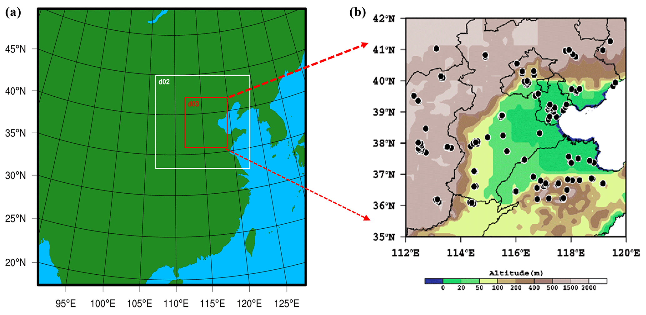
Figure 1 (a) Domain of the WRF-CMAQ model and (b) location of environmental monitoring stations in the innermost domain over the BTH region.

3 Inverse modeling method

3.1 Constructing the BEC matrix

To construct the BEC matrix for the inversion model, we combined the technique by the National Meteorological Center (NMC) (Parrish and Derber, 1992) with the SMOKE model based on uncertainty analysis of the ES inventories. We created the BEC matrix by four steps, as follows:

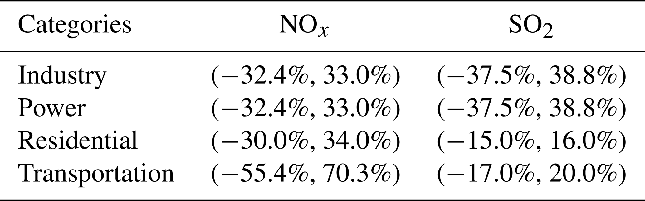
1. Determine the total errors of ES from an a priori bottom-up inventory. Uncertainty analyses of ESs require detailed information of activities and emission factors from an a priori MEIC emission inventory. The relevant data collected in the China Environmental Yearbook are limited and do not satisfy the requirements of uncertainty analysis. Therefore, we used the available research results relating to SO₂ and NO_x ESs and conducted uncertainty analysis for four types of major sources (industry, power plants, residents, and transportation) based on activities and emission factors from the references (Hong et al., 2017; Zheng et al., 2018; Peng et al., 2019) using the AuvTool software (Frey et al., 2002) and determined the error ranges in total emission rates of SO₂ and NO_x (Table 1). Uncertainties in SO₂ industry and power plant ESs are slightly greater than those for NO_x, while the opposite is true for emissions from the residential and traffic sectors.

2. Generate multiple sets of inventories using the random perturbation technique. Based on the aforementioned error ranges in total emission rates, we generated 30 sets of inventories for SO₂ and NO_x with the same resolution as MEIC for each month using a random perturbation method (Kerry et al., 2007). Firstly we obtain the probability distribution of errors of ESs based on uncertainty analysis for four sections, respectively. Then we conduct random perturbation on uncertainties of four sections of ES 30 times according to the probability distributions using the same perturbation coefficients for every perturbation. Lastly we calculate 30 total emission rates using random uncertainties of four sections for every set of inventories, respectively.

3. Process the 3D gridded ES as input to the CMAQ model. We used the SMOKE model, national population and road network distribution data in 2016, the temporal apportionment coefficients in the BTH region (Zhang et al., 2007; Wang et al., 2008), and the CB05-ae06-aq chemical species data in the CMAQ model, to process 30 sets of nationwide emission inventories into 3D gridded ES with a grid spacing of 5×5 km. Each grid has 124×130 points, with 12 vertical levels.

4. Calculate the BEC matrix of each 3D gridded ES. Finally, the NMC method was used to calculate the BEC matrix of the 3D gridded ES for each month, including horizontal and vertical correlation coefficients and standard deviations. The background error is defined as the difference between 30 sets of 3D gridded ESs generated by the random perturbation method and the 3D gridded background ES directly processed from the original MEIC emission inventory with the SMOKE model, at every hour (24 h diurnal variation of ES for every month).

Table 1 Uncertainty of NO_x and SO₂ values used in the SMOKE model and calculation of the BEC matrix.

According to the literature (Liu et al., 2011; Li et al., 2013; Zang et al., 2016), the approximate calculation of the BEC matrix is as follows:

$$\begin{array}{}\text{(1)}& \mathbf{B}\approx {\displaystyle \frac{\mathrm{1}}{\mathrm{2}}}\langle ({\mathit{e}}_t-{\mathit{e}}_{\mathrm{b}})({\mathit{e}}_t-e_{\mathrm{b}}{)}^{\mathrm{T}}\rangle ,\end{array}$$

where e_t is the perturbation field, and e_b is the background field of an a priori ES. Equation (1) can be written as follows:

$$\begin{array}{}\text{(2)}& \mathbf{B}={\mathbf{DC}}^{\mathrm{T}},\end{array}$$

where D is the standard deviation (SD) matrix, and C is the correlation coefficient matrix. With this factorization, D and C can be calculated separately. D is a diagonal matrix, whose elements are the SD of all state variables in the 3D grids. C is used to improve the ability of the 3DVAR in representing the impacts of local emissions at one grid on other grids; these impacts vary in the vertical direction, and they are heterogeneous in the horizontal direction.

Figure 2 shows the spatial distribution of averaged emission rates for 30 sets of 3D gridded ESs and the SD of the BEC matrix for SO₂ and NO_x ESs at 08:00 local time in December. SO₂ and NO_x ESs have different spatial distributions in terms of average strength and standard deviation. The NO_x emissions are mainly concentrated in cities and surrounding areas, and they are much greater in Beijing, Tianjin, and Shijiazhuang than other cities. The SO₂ emissions are mainly concentrated in Shijiazhuang, Jinan, the north and east of Shanxi Province, and their surrounding areas. Figure 3 shows variations in the horizontal correlation coefficients by grid distance and the vertical distributions of the SD in B for SO₂ and NO_x ESs in December 2012. The cross between the correlation curve and the $e^{-\mathrm{1}/\mathrm{2}}$ line (dashed line) represents the horizontal length scale (L_s), and the L_s of the two species falls between five and six grid distances. Namely, the horizontal scale felt is approximately 25–30 km. The correlation coefficient of SO₂ is slightly larger than that of NO₂. The difference in the correlation coefficients between SO₂ and NO_x ESsincreases with grid distance, and this is related to the regional pollution characteristics of SO₂. The vertical distributions of the SDs in B for SO₂ and NO_x ESs vary with height: the SDs of the SO₂ ES are larger on the fourth and eighth model levels than on other levels, while for the NO_x ES, the SD on the first level is the largest, that on the eighth level take the second place, and the SDs on all other levels are smaller.

Figure 2 Spatial distributions of (a) averaged emission rates of the SO₂ ES, (b) standard deviation in the BEC of the SO₂ ES, (c) averaged emission rates of the NO_x ES, and (d) standard deviation in the BEC of the NO_x ES at 08:00 local time in December 2012. Unit: mole/s.

Figure 3 (a) Horizontal correlation coefficients with increasing grid distance and (b) vertical profiles of standard deviations in the BEC of SO₂ and NO₂ ESs in December 2012. The dashed line is the baseline of the horizontal correlation scale.

3.2 Sensitivity analysis

The sensitivity analysis module (DDM-3D) in CMAQ solves a series of equations while simultaneously calculating pollutant concentrations. The local sensitivity of pollutant concentrations with respect to several specified parameters, such as the ES, initial and boundary conditions, and chemical reaction rates, can be calculated by the DDM-3D method. The sensitivity equations about the ES are solved using the governing equations of the model, as follows (Hu et al., 2009):

$$\begin{array}{}\text{(3)}& \mathbf{S}={\mathit{p}}_j{\displaystyle \frac{\partial \mathbf{C}}{\partial {\mathit{p}}_j}}={\mathit{p}}_j{\displaystyle \frac{\partial \mathbf{C}}{\partial \left({\mathit{\epsilon }}_j{\mathit{p}}_j\right)}}={\displaystyle \frac{\partial \mathbf{C}}{\partial {\mathit{\epsilon }}_j}},\end{array}$$

where S is the sensitivity of the pollutant j to the parameter p_j, p_j is an a priori ES of the pollutant j, C is the concentration of the pollutant j, and ε_j is the perturbation coefficient of the ES. Theoretically, the DDM-3D method truly captures the sensitivities of pollutant concentrations to ES, and results are more accurate than the brute force method, for the BTH region (Wang et al., 2013). In addition, the results of the DDM-3D method are more accurate and efficient for highly nonlinear pollutants (such as O₃ and PM_2.5) and small perturbations.

We used the WRFv3.7.1 and CMAQv5.0.2-DDM-3D models as well as 3D gridded a priori ES from MEIC in 2012 to calculate the sensitivity coefficients of SO₂ and NO₂ concentrations with respect to ESs during the heavy haze episode of 27–30 December 2016. Figure 4 shows the spatial distribution of 96 h averaged sensitivity coefficients for SO₂ and NO₂ concentrations with respect to ESs during 27–30 December 2016. The sensitivity coefficients of SO₂ and NO₂ concentrations all exhibit inhomogeneous distribution. The sensitivity coefficients are higher in Beijing, Shijiazhuang, Baoding, and surrounding regions; i.e., SO₂ and NO₂ concentrations in those areas are greatly affected by the SO₂ and NO_x ESs.

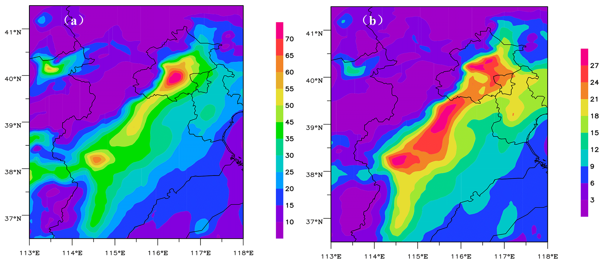
Figure 4 Spatial distributions of 96 h averaged sensitivity coefficients (µg m⁻³) of (a) SO₂ and (b) NO_x concentrations with respect to SO₂ and NO_x ESs during 27–30 December 2016.

3.3 Observation operators

The relationship between pollutant source and the receptor's concentration is established according to Eq. (3). Next, we create the observation operator matrix between the ES and receptor concentrations as follows:

$$\begin{array}{}\text{(4)}& \mathbf{H}={\displaystyle \frac{\partial \mathbf{C}}{\partial \mathbf{E}}}={\displaystyle \frac{\partial \mathbf{C}}{\partial \left({\mathit{\epsilon }}_j{\mathbf{E}}_{\mathrm{0}}\right)}}={\displaystyle \frac{\mathbf{S}}{{\mathbf{E}}_{\mathrm{0}}}},\end{array}$$

where H is the observation operator matrix, E denotes an a posteriori ES, which can be written as the product of the perturbation coefficient and an a priori ES during the assimilation window time, and E₀ denotes an a priori ES. For primary pollutants such as SO₂ and NO₂, S is a first-order sensitivity coefficient, and H is a linear observation operator between the ES and the receptor concentration. For secondary pollutants such as PM_2.5 and O₃, S is a high-order sensitivity coefficient, and H is a nonlinear observation operator. In this study, we use the first-order sensitivity coefficient to calculate H for SO₂ and NO_x ESs.

3.4 Observational error covariance

We firstly performed quality control on the observed SO₂ and NO₂ concentration data. This process involved three steps:

1. Redundant data were removed, and the density of observation data was matched to the model grid. For some grids with more than one observation station, we used the average of those stations.

2. Extrema were controlled; i.e., data exceeding 3 times the SD of observation data were filtered out.

3. Anomalies were removed; i.e., data that remained constant for 24 consecutive hours, as well as any negative data, were removed.

Data that passed quality control still contained observation or instrument errors. These errors are related to many factors such as instrument type, calibration design, and environmental conditions. In addition, in the variational assimilation process, representation errors caused by the forward-calculation and variational processes must be considered. Higher resolution models produce smaller representation errors. Representation error, ε_r, can be expressed as follows (Pagowski et al., 2010):

$$\begin{array}{}\text{(5)}& {\mathit{\epsilon }}_{\mathrm{r}}=\mathit{\gamma }{\mathit{\epsilon }}_{\mathrm{o}}\sqrt{{\displaystyle \frac{\mathrm{\Delta }x}{L_{\mathrm{s}}}}},\end{array}$$

where γ is the amplification factor, which is used to adjust the instrument error, ε_o is related to the SO₂ and NO₂ concentrations, and Δx is grid distance of the model. Note that L_s is usually smaller in urban areas and larger in suburban areas. The amplification parameters of the observing stations in cities, suburbs, and rural areas are 2.5, 5, and 10 km, respectively (Zang et al., 2016). Finally, the total observation error for the SO₂ and NO₂ concentrations, ε, is written as

$$\begin{array}{}\text{(6)}& \mathit{\epsilon }=\sqrt{{\mathit{\epsilon }}_{\mathrm{o}}^{\mathrm{2}}+{\mathit{\epsilon }}_{\mathrm{r}}^{\mathrm{2}}}.\end{array}$$

3.5 3DVAR inversion model

We introduce a cost function with respect to the ES in accordance with 3DVAR:

$$\begin{array}{}\text{(7)}& J\left(\mathit{e}\right)={\displaystyle \frac{\mathrm{1}}{\mathrm{2}}}{\left(\mathit{e}-{\mathit{e}}_{\mathrm{b}}\right)}^{\mathrm{T}}{\mathbf{B}}^{-\mathrm{1}}(\mathit{e}-{\mathit{e}}_{\mathrm{b}})+{\displaystyle \frac{\mathrm{1}}{\mathrm{2}}}{\left(\mathbf{H}\mathit{e}-\mathit{c}\right)}^{\mathrm{T}}{\mathbf{R}}^{-\mathrm{1}}\left(\mathbf{H}\mathit{e}-\mathit{c}\right),\end{array}$$

where c is the observation variable, R is the observation error matrix, and e is the inversing variable of an a posteriori ES. The optimal inversion of the ES for SO₂ and NO_x is obtained using Eq. (7). The 3DVAR solves for the minimum value of J(e) to determine the inversing variable e. This process typically employs a gradient propagation method, with the increment of an ES defined as follows:

$$\begin{array}{}\text{(8)}& \mathit{\delta }\mathit{e}=\mathit{e}-{\mathit{e}}_{\mathrm{b}}.\end{array}$$

Accordingly, the innovation vector of pollutant concentration is defined as

$$\begin{array}{}\text{(9)}& \mathit{\delta }\mathit{c}=\mathit{c}-\mathbf{H}{\mathit{e}}_{\mathrm{b}}.\end{array}$$

Therefore, Eq. (7) can be written in gradient form:

$$\begin{array}{}\text{(10)}& J\left(\mathit{\delta }\mathit{e}\right)={\displaystyle \frac{\mathrm{1}}{\mathrm{2}}}\mathit{\delta }{\mathit{e}}^T{\mathbf{B}}^{-\mathrm{1}}\mathit{\delta }\mathit{e}+{\displaystyle \frac{\mathrm{1}}{\mathrm{2}}}{\left(\mathbf{H}\mathit{\delta }\mathit{e}-\mathit{\delta }\mathit{c}\right)}^{\mathrm{T}}{\mathbf{R}}^{-\mathrm{1}}\left(\mathbf{H}\mathit{\delta }\mathit{e}-\mathit{\delta }\mathit{c}\right).\end{array}$$

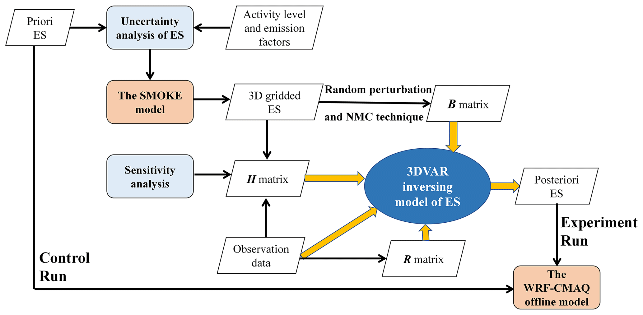
After conditionally processing the cost function, a finite-memory quasi-Newton method was used to conduct iterative minimization. The background field was set as the initial iteration values. The maximum number of steps at the end of the iteration and the minimum gradient for convergence were predetermined. The iteration was finished when one of these conditions was met, and the optimal analysis increment, δe, was obtained. Finally, the optimal assimilation analysis field of the ES, $\mathit{e}=\mathit{\delta }\mathit{e}+{\mathit{e}}_{\mathrm{b}}$, was obtained. The result was a three-dimensional variational inversion model of the ES, using the uncertainty analysis of the ES and sensitivity coefficients between the ES and the receptor's concentrations; the overall framework is shown in Fig. 5.

Figure 5 Flowchart of the 3DVAR inversion model of the ES and simulation experiments.

4 Results and discussion

A typical heavy haze event occurred in the BTH region at the end of December 2016. We applied the 3DVAR inversion model to constrain an hourly a posteriori ES of SO₂ and NO₂ using measurements from 45 and 129 stations, respectively, on 27 December 2016. We validated simulations from the control and experiment run using observational data during 28–30 December 2016.

Figure 6 shows time series of hourly, regional averaged SO₂ and NO₂ simulations from the control run, observations, and sensitivity coefficients at 45 stations in the BTH region during 27–30 December 2016. The trends in modeled concentrations and sensitivity coefficients of SO₂ and NO₂ concentrations with respect to the ES are consistent; therefore the sensitivity coefficients can reasonably reflect the impacts of the ES on concentrations. However, simulated SO₂ and NO₂ concentrations with an underestimated a priori ES are all significantly lower than observations during the heavy haze period. Thus, it is important to improve a priori ES using the inversion model.

Figure 6 Time series of hourly, regionally averaged (a) SO₂ and (b) NO₂ simulations with an a priori ES, observations, and the first-order sensitivity coefficients between the ES and the receptor's concentration at 45 stations over the BTH region during 27–30 December 2016.

Figures 7 and 8 show the spatial distributions of 24 h averaged emission rates from an a priori and a posteriori ES of SO₂ and NO₂ and their increments on 27 December 2016. Emission rates of a posteriori ES of SO₂ and NO₂ in the major cities and surrounding areas clearly increase. Compared with a priori ES, the maximum strengths of SO₂ and NO₂ ESs increase by approximately 17 % and 500 %, respectively. Therefore, the strengths of SO₂ and NO₂ in a priori ESs were greatly underestimated, especially for NO₂.

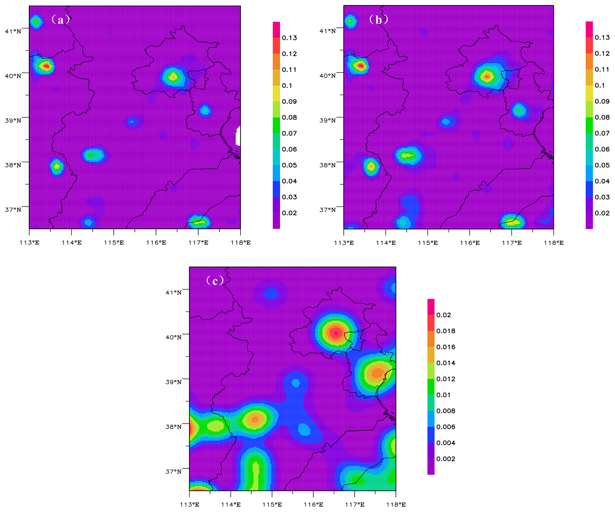
Figure 7 Spatial distributions of 24 h averaged emission rates for SO₂ (mole/s) from (a) a priori and (b) a posteriori ESs and (c) the increment on 27 December 2016.

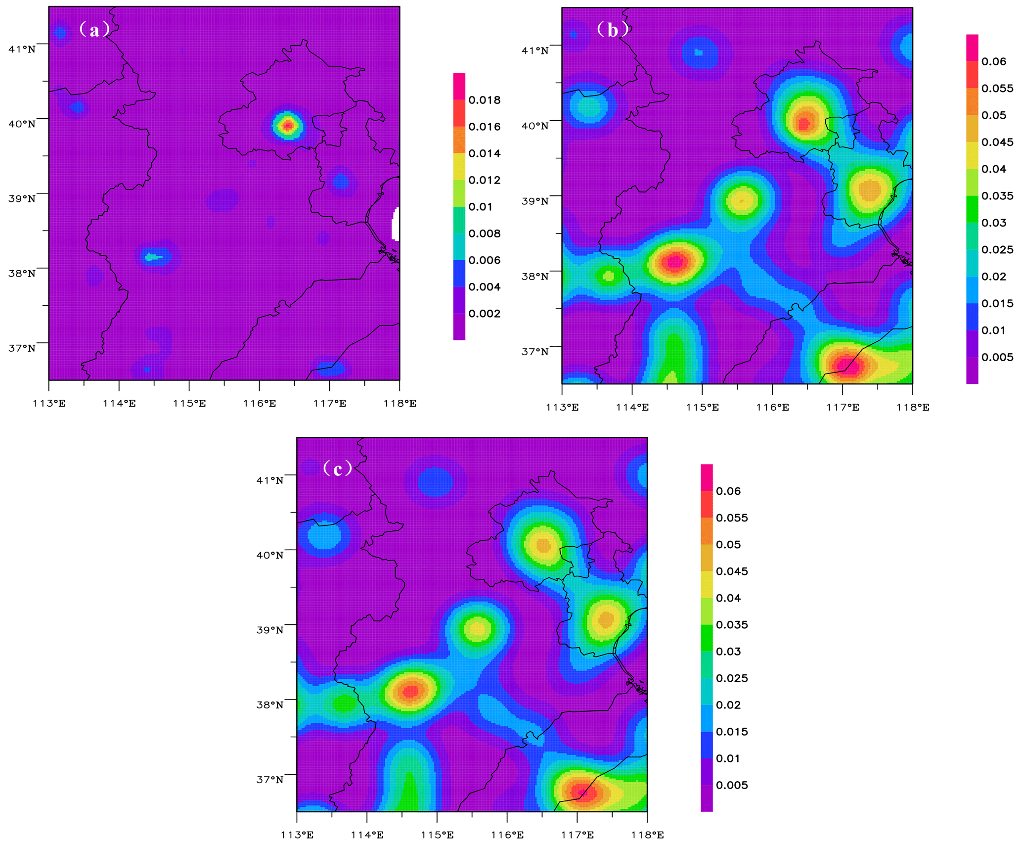
Figure 8 Same as Fig. 7 except for NO₂.

Using the WRF-CMAQ model and an a posteriori ES, we simulated concentrations of SO₂, NO₂, and O₃ in the BTH region during 28–30 December 2016 and validated these simulations with measurements from 45 stations. Figures 9 and 10 show the spatial distributions of 72 h averaged SO₂ and NO₂ concentrations simulated with a priori and a posteriori ESs, increments, and their observations. In general, SO₂ and NO₂ concentrations simulated using an a posteriori ES are closer to observations than an a priori ES, and regional differences in improvements for SO₂ and NO₂ exist. For SO₂, the improvement is noticeable in the BTH region. However, the simulated concentrations in Beijing with an a posteriori ES are overestimated. This may be related to greater uncertainties in SO₂ sources and the impacts of regional transport from surrounding areas. For NO₂, simulated differences with a priori and a posteriori ESs are significant in major cities such as Beijing, Tianjin, Shijiazhuang, Baoding, Xingtai, Handan, and Jinan. The simulated concentrations of NO₂ using a posteriori ES are more consistent with measurements, while those with a priori ES are significantly underestimated.

Figure 9 Spatial distribution of 72 h averaged SO₂ concentration simulated with (a) a priori and (b) a posteriori ESs and (c) the increment during 28–30 December 2016. Color solid dots denote the measurements.

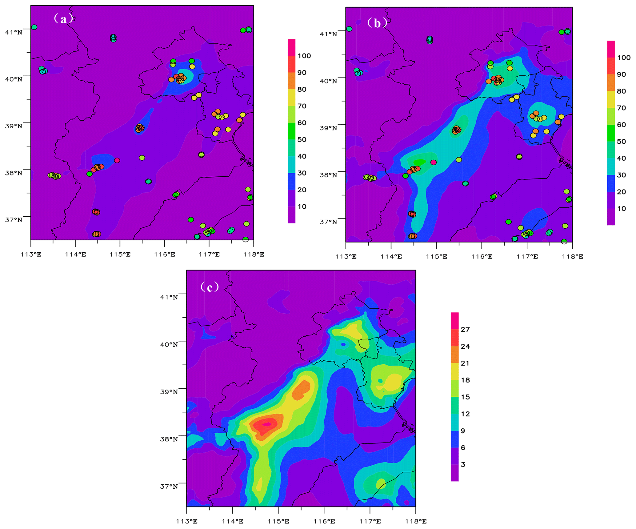
Figure 10 Same as Fig. 9 except for NO₂.

We also investigated temporal variations in regionally averaged SO₂, NO₂, and O₃ concentrations simulated using a priori and a posteriori ESs and observations from the 45 stations over the BTH region during 28–30 December 2016 (Fig. 11). In general, simulated SO₂, NO₂, and O₃ concentrations using an a posteriori ES are closer to measurements, while the SO₂ and NO₂ concentrations simulated by an a priori ES are significantly lower than observations, and the modeled O₃ concentrations are obviously higher than measurements. In addition, the peak of SO₂ simulations with an a posteriori ES is close to measurements, but the peak of NO₂ and valley of O₃ simulations are lower and higher than observations, respectively. This may be related to the absence of inverse modeling of a volatile organic compound (VOC) ES and the uncertainties of sensitivity coefficients calculation. In this study, we used only first-order sensitivity coefficients, but the relationship between the ES of precursors of O₃ such as VOCs and NO_x and their receptor's concentrations is nonlinear, and O₃ is generated from both the NO_x and VOC ES. Therefore, higher order sensitivity coefficients are necessary for the inverse modeling of the ES of NO_x and VOCs.

Figure 11 Time serial of regional averaged (a) SO₂, (b) NO₂, and (c) O₃ concentrations respectively simulated with a priori and a posteriori ESs, and measurements at 45 stations in the BTH region during 28–30 December 2016.

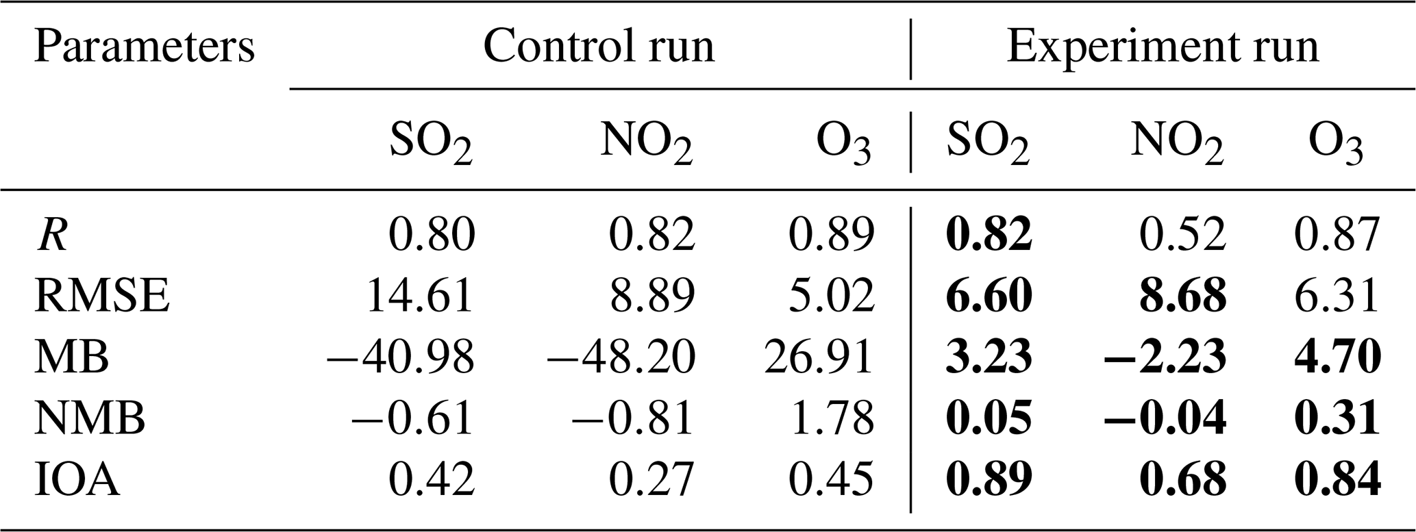
To further assess the simulated accuracy of SO₂, NO₂, and O₃ concentrations, we calculated the following statistics (Willmott et al., 2012): correlation coefficient (R), root-mean-squared error (RMSE), mean bias (MB), normalized mean bias (NMB), and index of agreement (IOA; see Table 2). Except the result that R values of NO₂ and O₃ decrease and the RMSE of O₃ increases using the constrained ES, other statistics show improvements. In particular, MB and NMB of three pollutants decline significantly, and IOA is closer to 1.0, which means that modeled results of the three pollutants are more consistent with observations. R between SO₂ simulation and observation shows a slight improvement when using an a posteriori ES, whereas R decreases for NO₂ and O₃, and it may be related with the absence of constraint of a VOC ES.

Table 2 Statistics for simulated SO₂, NO₂, and O₃ from control and experiment runs using a priori and a posteriori inversed ESs at 45 stations in the BTH region during 28–30 December 2016. Bold type indicates better statistical results.

5 Summary and conclusions

We developed a new inverse approach of ES by combining the sensitivity analysis technique between the ES and the receptor's concentration and the 3DVAR method. Our approach is suitable for solving the linear or nonlinear inversion problems for ESs It computes quickly and obtains relatively accurate real-time dynamic updates of ESs. First, we used the sensitivity analysis tool in the CMAQ model to construct the explicit observation operator matrix between the ES and the receptor's concentration. Next, we created the BEC matrix for ES based on uncertainty analysis and the NMC statistical method. Finally, we established a three-dimensional variational inverse method of ES based on the observation operator and BEC matrix.

The 3DVAR inversion model was applied to a heavy haze case study in the BTH region during 27–30 December 2016. Results show that the observation operators between SO₂ and NO₂ ESs and their concentrations, as well as spatial distributions of the BEC matrix, are both reasonable. Using the 3DVAR inversion model, a priori SO₂ and NO₂ ESs improved obviously during the heavy haze process, especially for the NO₂ ES. The spatial distributions of SO₂ and NO₂ concentrations simulated using an a posteriori ES are more consistent with measurements than an a priori ES, especially in major cities over the BTH region. Simulation errors of SO₂, NO₂, and O₃ concentrations with an a posteriori ES significantly decrease, whereas simulations of three pollutants using an a priori ES are underestimated.

Large discrepancies of the simulation and sensitivity coefficient over December 29 may be related with absent calculation of high-order sensitivity coefficient in this case. In the future, we will adopt high-order sensitivity coefficient to improve the constraint effect of SO₂ and NO_x emission sources. In addition, future studies will include the applicability and accuracy of this method for different seasons and regions and different chemical species such as other primary pollutants (e.g., CO) and precursors of secondary pollutants (e.g., PM_2.5, PM₁₀, and O₃). An emphasis may be placed on constructing the nonlinear explicit observation operator for precursors of secondary pollutants such as a VOC ES using the high-order sensitivity analysis technique and assessing improvement effects of an a posteriori ES with the 3DVAR inversion method and the CMAQ model.