Quantification of uncertainties in the assessment of an atmospheric release source applied to the autumn 2017 ¹⁰⁶Ru event

Using a Bayesian framework in the inverse problem of estimating the source of an atmospheric release of a pollutant has proven fruitful in recent years. Through Markov chain Monte Carlo (MCMC) algorithms, the statistical distribution of the release parameters such as the location, the duration, and the magnitude as well as error covariances can be sampled so as to get a complete characterisation of the source. In this study, several approaches are described and applied to better quantify these distributions, and therefore to get a better representation of the uncertainties. First, we propose a method based on ensemble forecasting: physical parameters of both the meteorological fields and the transport model are perturbed to create an enhanced ensemble. In order to account for physical model errors, the importance of ensemble members are represented by weights and sampled together with the other variables of the source. Second, once the choice of the statistical likelihood is shown to alter the nuclear source assessment, we suggest several suitable distributions for the errors. Finally, we propose two specific designs of the covariance matrix associated with the observation error. These methods are applied to the source term reconstruction of the ¹⁰⁶Ru of unknown origin in Europe in autumn 2017. A posteriori distributions meant to identify the origin of the release, to assess the source term, and to quantify the uncertainties associated with the observations and the model, as well as densities of the weights of the perturbed ensemble, are presented.

1 Introduction

1.1 Bayesian inverse modelling for source assessment

The inverse modelling of a nuclear release source is an issue fraught with uncertainties (Abida and Bocquet, 2009). Variational techniques (Saunier et al., 2013; Bocquet, 2012), which only provide a deterministic and thus unique solution to the problem, miss valuable information such as other potential sources. On the other hand, probabilistic methods develop stochastic solutions able to capture all information from the data. In particular, Bayesian methods have proven to be very efficient in source term estimation (STE) problems. Several techniques such as the iterative variational Bayes method (Tichý et al., 2016) tested using data from the European Tracer Experiment (ETEX), or an adaptive scheme based on importance sampling (Rajaona et al., 2015) and tested on the Fusion Field Trials 2007 experiment, have been developed. Sampling using Markov chain Monte Carlo (MCMC) methods is a very popular technique, since it allows the posterior distribution of the source to be directly assessed. It has been applied by Delle Monache et al. (2008) to estimate the Algeciras incident source location. Keats et al. (2007) sampled the source parameters of a complex urban environment with the help of the Metropolis–Hastings algorithm. The emissions of xenon-133 from the Chalk River Laboratories medical isotope production facility were reconstructed with their location by Yee et al. (2014). Various Bayesian methods including MCMC techniques are used by Liu et al. (2017) to assess the source term of the Chernobyl and Fukushima Daiichi accidents and their associated uncertainties.

1.2 Ensemble methods

A major source of uncertainties in the inverse modelling for source term estimation of nuclear accidents originates from the meteorological fields and the transport models (Sato et al., 2018) which are used to simulate the plume of the emission. Weather forecast uncertainties arise from errors in the initial conditions and approximations in the construction of the numerical model. They can be evaluated through the use of an ensemble forecast (Leith, 1974). Several realisations of the same forecast are considered, where for each realisation, the initial condition and the numerical model are perturbed. These forecasts can then be combined to generate a single forecast. More specifically, ensemble members can be linearly combined, where each member of the ensemble is given a weight. In a deterministic approach, weights can be computed using assorted methods such as machine learning (Mallet et al., 2009) or least squares algorithms (Mallet and Sportisse, 2006). For weather forecasting, these weights can depend on past observations or analyses (Mallet, 2010). As developed later in this paper in Sect. 2.3, the study of the weights provides access to the uncertainty in meteorological models. The uncertainty due to the transport model can also be studied through ensemble methods such as that of Delle Monache and Stull (2003), who use a mixture of diverse air quality models. We propose in this paper a new technique to estimate the weights associated with ensemble members.

1.3 Probabilistic description of the problem

We wish to parametrise the distribution of the variable vector x describing the source of a release. In the case of a point-wise source of unknown location, the most important variables describing the source are the coordinates longitude–latitude (x₁,x₂), the vector ln q (where each component corresponds to the logarithm of the release q on a given time interval, e.g. an hour or a day), and the covariance matrix R containing the model–measurement error variances defined below. The posterior probability distribution is written with the help of Bayes' theorem as

$$\begin{array}{}\text{(1)}& {\displaystyle }{\displaystyle }p\left(\mathit{x}\right|\mathit{y})={\displaystyle \frac{p\left(\mathit{y}\right|\mathit{x}\left)p\right(\mathit{x})}{p\left(\mathit{y}\right)}}\propto p(\mathit{y}\left|\mathit{x}\right)p\left(\mathit{x}\right),\end{array}$$

with y the observation vector, usually a set of air concentration measurements, and x the source variable vector. The first term p(y|x) of Eq. (1) corresponds to the likelihood distribution quantifying the fit of a statistical model (here the characterisation of the source x) with the data (the observation vector y). The second term, the prior p(x), describes the probability distribution of prior knowledge on the source vector before considering data. Once the posterior probability distribution is known up to a normalisation constant, several sampling techniques can be applied to it (Liu et al., 2017).

The shape of the posterior distribution strongly depends on the uncertainties related to the data and the modelling choices, which include the meteorological data and transport models definitions as well as the likelihood definition. The objective of this study is to investigate the various sources of uncertainties compounding the problem of source reconstruction, and to propose solutions to better evaluate them, i.e. to increase our confidence in the reconstructed posterior distribution. The quantification of the uncertainties largely depends on the definition of the likelihood and its components (for example, a corresponding covariance matrix). The choice of the likelihood is the concern of Sect. 2.1. As mentioned above, the likelihood term quantifies the fitness between the measurements y and a given transformation of the source x. To make these two quantities comparable, a set of modelled concentrations corresponding to the observations are computed. These concentrations, also called predictions, are the results of a simulation of the dispersion of the source x and depend on the parametrisation of the transport model and on the meteorological fields.

In this paper and in the case of a source of unknown location, the predictions are written as ${\mathit{y}}_S={\mathbf{H}}_{x_{\mathrm{1}},x_{\mathrm{2}}}\mathit{q}$ where H is the observation operator, the matrix representing the resolvent of the atmospheric transport model, and ${\mathbf{H}}_{x_{\mathrm{1}},x_{\mathrm{2}}}$ its definition for a source of coordinates x₁,x₂. Therefore, the observation operator does vary linearly with q. However, H is not linear in the coordinates. When the coordinates are unknown, they may be investigated in a continuous space. The computation of a matrix ${\mathbf{H}}_{x_{\mathrm{1}},x_{\mathrm{2}}}$ for a specific couple of coordinates being expensive, a set of observation operators linked to specific locations is computed on a regular mesh G prior to the Bayesian sampling presented in Sect. 3.2.3. The observation operators are therefore interpolated from the set of observation operators pre-computed on G.

Equation (1) can be expanded as

$$\begin{array}{ll}{\displaystyle }& {\displaystyle }p\left(\mathit{x}\right|\mathit{y})\propto \\ \text{(2)}& {\displaystyle }& {\displaystyle }{p}_{\text{likelihood}}\left(\mathit{y}\right|{\mathbf{H}}_{x_{\mathrm{1}},x_{\mathrm{2}}}\left(m\right)\mathit{q},\mathbf{R}\left)p_{\text{prior}}\right(x_{\mathrm{1}},x_{\mathrm{2}},\ln \mathit{q},\mathbf{R}),\end{array}$$

where uncertainties are embodied in

• the observations y;

• the physical models: the meteorological fields m and the dispersion H;

• the likelihood definition: its choice and the design of its associated error covariance matrix R;

• the representation error: the release rates q as a discrete vector (while the release is a continuous phenomenon), the observation operator ${\mathbf{H}}_{x_{\mathrm{1}},x_{\mathrm{2}}}$ as an interpolation, and the observations for which the corresponding predictions are calculated in a mesh containing them;

• the choice of the priors.

In this paper, we focus on the uncertainties emanating from the physical models and the definition of the likelihood.

1.4 Objectives of this study

This study is a continuation from a previous study from the authors (Dumont Le Brazidec et al., 2020). It aims to explore the various sources of uncertainty which are compounding the inverse problem and propose solutions to better evaluate them: three key issues are investigated. First, in Sect. 2.1, we investigate the design of the likelihood distribution, which is a key ingredient in the definition of the posterior distribution. Second, we propose two new designs of the likelihood covariance matrix to better evaluate errors in Sect. 2.2. Finally, in Sect. 2.3, we describe an ensemble-based method for taking into account the uncertainties related to the meteorological fields and atmospheric transport model: H is built as a weighted sum of observation operators created out of diverse physical parameters.

Subsequently, these three sources of uncertainty are explored in an application of source term estimation of the ¹⁰⁶Ru release in September 2017. First, a description of the context, the observation dataset, and the release event are provided in Sect. 3.1. Then the parametrisation of the physical model is presented in Sect. 3.2.1. Finally, the results of the successive applications of the assorted methods described in Sect. 2, combined or not, are presented in Sect. 3.3. A summary of the various configurations of each application is proposed in Sect. 3.3.1. Conclusions on the contribution of each method are finally proposed.

2 Evaluating uncertainties in the Bayesian inverse problem

2.1 Choice of the likelihood

In the field of source assessment, and more precisely radioactive material source assessment, the likelihoods are often defined as Gaussian (Yee, 2008; Winiarek et al., 2012; Saunier et al., 2013; Bardsley et al., 2014; Yee et al., 2014; Winiarek et al., 2014; Rajaona et al., 2015; Tichý et al., 2016), or adapted from a Gaussian to consider non-detections and false alarms (De Meutter and Hoffman, 2020), or more recently log-normal (Delle Monache et al., 2008; Liu et al., 2017; Saunier et al., 2019; Dumont Le Brazidec et al., 2020) or akin to a log-normal (Senocak et al., 2008). The multivariate Gaussian probability density function (pdf) of y, of mean Hx and covariance matrix R, is written as

$$\begin{array}{}\text{(3)}& {\displaystyle }{\displaystyle }p\left(\mathit{y}\right|\mathit{x})={\displaystyle \frac{\mathrm{1}}{\sqrt{\mathrm{2}\mathit{\pi }\left|\mathbf{R}\right|}}}\text{exp}\left(-{\displaystyle \frac{(\mathit{y}-\mathbf{H}\mathit{x}{)}^{\top }{\mathbf{R}}^{-\mathrm{1}}(\mathit{y}-\mathbf{H}\mathit{x})}{\mathrm{2}}}\right).\end{array}$$

In this section, we assume that the covariance matrix R is equal to rI, where r is a positive coefficient. The cost function, i.e. the negative of the log-likelihood, of the Gaussian probability density function (pdf) is written (up to a normalisation constant) as

$$\begin{array}{}\text{(4)}& {\displaystyle }{\displaystyle }{\mathcal{J}}_{\mathit{y}}\left(\mathit{x}\right)=-\ln p\left(\mathit{y}\right|\mathit{x})={\displaystyle \frac{N_{\text{obs}}\ln r}{\mathrm{2}}}+{\displaystyle \frac{(\mathit{y}-\mathbf{H}\mathit{x}{)}^{\top }(\mathit{y}-\mathbf{H}\mathit{x})}{\mathrm{2}r}},\end{array}$$

with N_obs the number of observations. The cost function is a matter of judgement; it measures how detrimental a difference between an observation and a prediction is. When the observations and the predictions are equal, the cost corresponding to the likelihood should be zero and it should increase when the difference between the observation and the prediction values grows.

With the assumption R=rI, choosing a Gaussian likelihood penalises the largest errors to an extent that smaller errors are negligible: the Gaussian cost function value of an observation–prediction couple ($y=\mathrm{100}\mathrm{mBq}{\mathrm{m}}^{-\mathrm{3}},y_S=\mathrm{120}\mathrm{mBq}{\mathrm{m}}^{-\mathrm{3}}$) is a hundred of times greater than of ($y=\mathrm{10}\mathrm{mBq}{\mathrm{m}}^{-\mathrm{3}},y_S=\mathrm{12}\mathrm{mBq}{\mathrm{m}}^{-\mathrm{3}}$). In other words, with a Gaussian likelihood and the assumption R=rI, inverse modelling is dominated by the most significant measurements in real-case studies.

The whole set of measurements should provide information: if the inversion is dominated by the few measurements with the largest errors (which may possibly be outliers), valuable information provided by the other measurements may be missed. More generally, the following inventory lists the criteria that a good likelihood choice under the assumption R=rI (or any important simplification of R) for nuclear source assessment should fulfil:

• positive domain of definition: should be defined for values on the semi-infinite interval $[\mathrm{0},+\mathrm{\infty })$ since the observations and predictions are all positive by nature;

• symmetry between the prediction vector and the observation vector, i.e. $p(\mathit{y};\mathbf{H}\mathit{x},\mathbf{R})=p(\mathbf{H}\mathit{x};\mathit{y},\mathbf{R})$. The couple $\left(y=\mathrm{20}\mathrm{mBq}{\mathrm{m}}^{-\mathrm{3}},y_S=\mathrm{40}\mathrm{mBq}{\mathrm{m}}^{-\mathrm{3}}\right)$ should have the same penalty as $\left(y=\mathrm{40}\mathrm{mBq}{\mathrm{m}}^{-\mathrm{3}},y_S=\mathrm{20}\mathrm{mBq}{\mathrm{m}}^{-\mathrm{3}}\right)$;

• close to proportionality: the ratio of the cost function value of a couple $(\mathrm{20}\mathrm{mBq}{\mathrm{m}}^{-\mathrm{3}},\mathrm{40}\mathrm{mBq}{\mathrm{m}}^{-\mathrm{3}})$ with a couple $(\mathrm{200}\mathrm{mBq}{\mathrm{m}}^{-\mathrm{3}},\mathrm{400}\mathrm{mBq}{\mathrm{m}}^{-\mathrm{3}})$ should be close to 1 as a general rule. This criterion is a simplification since the distribution of errors might be more complex than simply multiplicative;

• existence of a covariance matrix, and of a term able to play the role of the modelled predictions. Indeed, the likelihood measures the difference between the observations and the predictions, which should therefore appear as a parameter of the distribution. Distributions with a location parameter comply with this requirement.

In particular, three distributions were found to satisfy these diverse criteria: the log-normal distribution already used in several studies, the log-Laplace and the log-Cauchy distributions, which have for cost functions (up to a normalisation constant) (Satchell and Knight, 2000; McDonald, 2008).

$$\begin{array}{ll}{\displaystyle }& {\displaystyle }{\mathcal{J}}_{\text{log-normal}}(\mathit{y};\mathbf{H}\mathit{x},\mathbf{R},{\mathit{y}}_{\mathbf{t}})=\\ \text{(5a)}& {\displaystyle }& {\displaystyle \frac{\mathrm{1}}{\mathrm{2}}}\Vert \ln (\mathit{y}+{\mathit{y}}_{\mathbf{t}})-\ln (\mathbf{H}\mathit{x}+{\mathit{y}}_{\mathbf{t}}){\Vert }_{\mathrm{2},{\mathbf{R}}^{-\mathrm{1}}}^{\mathrm{2}}+{\displaystyle \frac{N_{\text{obs}}}{\mathrm{2}}}\ln \left(r\right),{\displaystyle }& {\displaystyle }{\mathcal{J}}_{\text{log-Laplace}}(\mathit{y};\mathbf{H}\mathit{x},\mathbf{R},{\mathit{y}}_{\mathbf{t}})=\\ \text{(5b)}& {\displaystyle }& {\displaystyle }\Vert \ln (\mathit{y}+{\mathit{y}}_{\mathbf{t}})-\ln (\mathbf{H}\mathit{x}+{\mathit{y}}_{\mathbf{t}}){\Vert }_{\mathrm{1},{\mathbf{R}}^{-\mathrm{1}}}+N_{\text{obs}}\ln \left(r\right),{\displaystyle }& {\displaystyle }{\mathcal{J}}_{\text{log-Cauchy}}(\mathit{y};\mathbf{H}\mathit{x},\mathbf{R},{\mathit{y}}_{\mathbf{t}})=\\ \text{(5c)}& {\displaystyle }& {\displaystyle }\sum _{i=\mathrm{1}}^{N_{\text{obs}}}\ln \left(r+{\left(\ln (y_i+y_{\mathrm{t}})-\ln \left(\right(\mathbf{H}\mathit{x}{)}_i+y_{\mathrm{t}})\right)}^{\mathrm{2}}\right)-{\displaystyle \frac{\mathrm{1}}{\mathrm{2}}}\ln \left(r\right),\end{array}$$

where y_t is a positive threshold vector to ensure that the logarithm function is defined for zero observations or predictions. The l₂ and l₁ norms are defined as $\Vert \mathit{v}{\Vert }_{\mathrm{2},{\mathbf{R}}^{-\mathrm{1}}}=\sqrt{{\mathit{v}}^{\top }{\mathbf{R}}^{-\mathrm{1}}\mathit{v}}$ and $\Vert \mathit{v}{\Vert }_{\mathrm{1},{\mathbf{R}}^{-\mathrm{1}}}={\sum }_i\frac{\left|v_i\right|}{r_i}$ with R diagonal, respectively. These three distributions are subsumed by the generalised beta prime (or GB2) (Satchell and Knight, 2000; McDonald, 2008) and share a common point; all three are shaped around the subtraction of the logarithm of the observation by the logarithm of the prediction. Due to the logarithmic property $\ln \frac{a}{b}=\ln \left(a\right)-\ln \left(b\right)$, several criteria previously defined are met. First, the cost is a function of the ratio of the observation to the prediction. Second, these functions are defined with a location parameter which plays the role of the modelled prediction ln ((Hx)_i+y_t). And finally, with the help of a square or an absolute value, a symmetry between the observation and the prediction is guaranteed. Each of these choices requires a threshold (and even two for the log-Cauchy case, discussed at the end of this section) whose value significantly impacts the results. The log-normal and log-Cauchy distributions are compared for Bayesian source estimation by Wang et al. (2017).

Their difference lies in the treatment of the relative quantity $\ln (y_i+y_{\mathrm{t}})-\ln \left(\right(\mathbf{H}\mathit{x}{)}_i+y_{\mathrm{t}})$. With the l₂ norm, the log-normal drives most of the penalty on the large (relative) differences and removes almost all penalty from the small differences. With the l₁ norm, the log-Laplace curve of the relative quantity is flatter in comparison. This translates in the fact that the inverse modelling will not be sensitive to one couple in particular, even if for this couple the difference between the observation and the prediction is large. The motive therefore for using log-Laplace is to avoid having outliers driving the entire sampling, i.e. driving the entire search of the source. The log-Cauchy distribution is the one with the most interesting behaviour and mixes log-normal and log-Laplace natures. The logarithm mitigates the penalty of large differences but also removes any penalty from the small differences. The rationale of using the log-Cauchy distribution is consequently to avoid outliers, but at the same time to avoid taking into account negligible differences.

For all choices, the value of y_t is crucial to evaluate the penalty on a couple involving a zero observation or prediction. In other words, it calculates how the cost of a zero observation and a non-zero prediction (or the contrary) should compare to a positive couple. We consider that the penalty on a couple $(\mathrm{20}\mathrm{mBq}{\mathrm{m}}^{-\mathrm{3}},\mathrm{0}\mathrm{mBq}{\mathrm{m}}^{-\mathrm{3}})$ should be a large multiple of the penalty on $(\mathrm{400}\mathrm{mBq}{\mathrm{m}}^{-\mathrm{3}},\mathrm{100}\mathrm{mBq}{\mathrm{m}}^{-\mathrm{3}})$. As a consequence, it can be deduced that a “good” threshold for the log-normal distribution in a case involving important quantities released should lie between 0.5 and 3 mBq m⁻³. Using the same principle, acceptable thresholds for the log-Laplace or the log-Cauchy distributions range between 0.1 and 0.5 mBq m⁻³.

We should also consider that the log-Cauchy distribution needs a second threshold j_t to be properly defined. Indeed, if for a couple both observation y_i and prediction (Hx)_i are equal (usually both equal to zero), then r will naturally tend towards 0 so that 𝒥_log-Cauchy tends to −∞ as can be seen in Eq. (6) with j_t equal to zero. To prevent that, we can define j_t=0.1 mBq m⁻³ and

$$\begin{array}{ll}{\displaystyle }& {\displaystyle }{\mathcal{J}}_{\text{log-Cauchy}}(\mathit{y};\mathbf{H}\mathit{x},r,y_{\mathrm{t}})=\\ \text{(6)}& {\displaystyle }& {\displaystyle }\sum _{i=\mathrm{1}}^{N_{\text{obs}}}\ln \left(r+{\displaystyle \frac{{\left(\ln (y_i+y_{\mathrm{t}})-\ln \left(\right(\mathbf{H}\mathit{x}{)}_i+y_{\mathrm{t}})\right)}^{\mathrm{2}}}{r}}+{\displaystyle \frac{j_t}{c_{\text{ref}}}}\right),\end{array}$$

with c_ref=1 mBq m⁻³.

As will be shown later, the choice of the likelihood has in practice a significant impact on the shape of the posterior distribution. Hence, to better describe the uncertainties of the problem, the approach proposed here is to combine and compare the distributions obtained with these three likelihoods.

2.2 Modelling of the errors

The likelihood definition, and therefore the posterior distribution shape, is also greatly impacted by the modelling choice of the error covariance matrix R. The matrix is of size N_obs×N_obs. In real nuclear case studies, the number of observations can be important, whereas Bayesian sampling methods can usually estimate efficiently only a limited number of variables. To limit the number of variables, most of the literature (Chow et al., 2008; Delle Monache et al., 2008; Winiarek et al., 2012; Saunier et al., 2013; Rajaona et al., 2015; Tichý et al., 2016; Liu et al., 2017) describes the error covariance matrix as a diagonal matrix with a unique and common diagonal coefficient. This variance accounts for the observation (built-in sensor noise and bias), models (uncertainty of the meteorological fields and transport model), and representation error between an observation and a modelled prediction (e.g. Rajaona et al., 2015). Saunier et al. (2019) analyse the impact of such a choice on the same case study as this paper. Indeed, the error is a function of time and space and is obviously not common for every observation–prediction couple.

This critical reduction can lead to paradoxes. With R=rI, the variance r captures an average of the observation–prediction couples error variances. As seen in Appendix A, some observations can tamper the set of measurements and artificially reduce the value of r, which prevents the densities of the variables being well spread. Specifically, let us consider the non-discriminant observations. These are observations for which, for any probable source x, the observation is almost equal to the prediction. In other words, a non-discriminant observation is an observation which never contributes to discriminating any probable source from another. It is an observation for which, if R was modelled as a diagonal matrix with N_obs independent terms, the variance r_i corresponding to this observation would be very small or zero. If we model R as rI, then r, capturing an average of the N_obs variances r_i, decreases artificially. To deal with the existence of these observations, we propose to use two variances r₁ and r_nd. The discriminant observations will be associated with the variance r₁ while the non-discriminant observations will be associated with the variance r_nd during the sampling process. Necessarily then, r_nd tends to a very small value.

In the following, we refer to this algorithm as the observation-sorting algorithm. A justification of the use of this clustering using the Akaike information criterion (AIC) is proposed in Appendix B.

We now propose a second approach to improve the design of the covariance matrix R and the estimation of the uncertainties. We propose to cluster observations according to their spatial position in k groups, where observations of the same cluster are assigned the same observation error variance. This proposal is based on the fact that the modelling part of the observation error is a spatially dependent function. With this clustering, we have $\mathit{x}=(x_{\mathrm{1}},x_{\mathrm{2}},\ln \mathit{q},r_{\mathrm{1}},\mathrm{\dots },r_k)$ the source variables of interest, and R as a diagonal matrix where the ith diagonal coefficient is assigned a r_j with $j\in \mathit{\{}\mathrm{1},..,k\mathit{\}}$ according to the cluster to which the observation y_i belongs.

Using both methods, the set of variable x to retrieve becomes $(x_{\mathrm{1}},x_{\mathrm{2}},\ln \mathit{q},r_{\mathrm{1}},\mathrm{\dots },r_k,r_{\text{nd}})$.

2.3 Modelling of the meteorology and transport

As explained in Sect. 1.3, the linear observation operator H is computed with an atmospheric transport model, which takes meteorological fields as inputs. More precisely, the Eulerian ldX model, a part of IRSN's C3X operational platform (Tombette et al., 2014), validated on the Algeciras incident and the ETEX campaign, as well as on the Chernobyl accident (Quélo et al., 2007) and the Fukushima accident (Saunier et al., 2013), is the transport model used to simulate the dispersion of the plume, and therefore to build the observation operators. To improve the accuracy of the predictions, and therefore reduce the uncertainties, several observation operators computed with various physical parameters configuring the transport model and meteorological fields can be linearly combined. This combination then produces a single prediction forecast, hopefully more skilful than any individual prediction forecast.

First, ensemble weather forecasts can be used to represent variability in the meteorological fields. The members of the ensemble are based on a set of N_m models, where each model can have its own physical formulation. Second, considering a meteorology with little rainfall, three parameters of the transport model in particular can have an important impact on the dispersion of a particle (Girard et al., 2014) and are subject to significant uncertainties: the dry deposition, the height of the release, and the value of the vertical turbulent diffusion coefficient (Kz).

Therefore, to create an ensemble of observation operators with both uncertainty in the meteorological fields and in the transport parametrisation, a collection of observation operators ${\mathbf{H}}_{\mathrm{1}},\mathrm{\dots },{\mathbf{H}}_{N_e}$ can be computed out of four parameters. More specifically, each H_i with $i\in \mathit{\{}\mathrm{1},N_e\mathit{\}}$ is the output of a transport model parametrised by

• choosing a member from an ensemble of meteorological fields and hence a discrete value in [1,N_m];

• a constant deposition velocity in $[v_{\mathrm{d},\text{min}}=\mathrm{0.5}\times {\mathrm{10}}^{-\mathrm{3}}\mathrm{m}{\mathrm{s}}^{-\mathrm{1}},v_{\mathrm{d},\text{max}}=\mathrm{5}\times {\mathrm{10}}^{-\mathrm{3}}\mathrm{m}{\mathrm{s}}^{-\mathrm{1}}]$;

• a distribution of the height of the release between two layers defined between 0 and 40 m, and between 40 and 120 m, the space being discretised vertically in layers of various heights as described in Table 1;

• a multiplicative constant on the Kz values chosen in [0.333,3],

where each parameter range has been set up based on the work of Girard et al. (2014), and deposition and Kz processes are described in Table 1. The ensemble of observation operators is therefore computed from a collection of parameters. This collection is obtained from sampling the values of the parameters inside the intervals.

Once the set of operators has been built, the idea is to combine them linearly to get a more accurate forecast. A weight w_i can be associated with each observation operator of the ensemble:

$$\begin{array}{}\text{(7)}& {\displaystyle }{\displaystyle }{\mathit{y}}_S=\mathbf{H}\mathit{x}=\sum _{i=\mathrm{1}}^{N_e}{w}_i{\mathbf{H}}_i\mathit{x}=\sum _{i=\mathrm{1}}^{N_e}{w}_i{\mathit{y}}_{S,i},\end{array}$$

which results in combining linearly the predictions of each member of the ensemble. Each weight w_i is a positive variable to be retrieved. The weights can be included in the set of variables sampled by the MCMC algorithm. They are dependent on each other through the necessary condition ${\sum }_{i=\mathrm{1}}^{N_e}{w}_i=\mathrm{1}$ so this means N_e−1 weight variables will be added to $\mathit{x}=\left(x_{\mathrm{1}},x_{\mathrm{2}},\ln \mathit{q},\mathbf{R},w_{\mathrm{1}},\mathrm{\dots },w_{N_e-\mathrm{1}}\right)$.

Several methods are used in Sect. 3.3.4 to explore reliability, accuracy (level of agreement between forecasts and observations), skill, discrimination (different observed outcomes can be discriminated by the forecasts), resolution (observed outcomes change as the forecast changes), and sharpness (tendency to forecast extreme values) of probabilistic forecasts (Delle Monache et al., 2006). Rank histograms are used to evaluate the spread of an ensemble. Reliability diagrams (graphs of the observed frequency of an event plotted against the forecast probability of an event) and ROC curves (which plot the false positive rate against the true positive rate using several probability thresholds) are used to measure the ability of the ensemble to discriminate (Anderson, 1996).

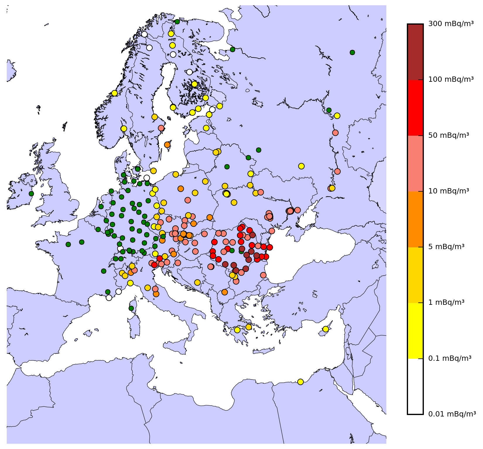
Figure 1 Maximum air concentrations of ¹⁰⁶Ru observed over Europe in mBq m⁻³. Green points measured concentrations below the detection limit.

Louis, 1979Troen and Mahrt, 1986Baklanov and Sørensen (2001)

Table 1 Main configuration features of the ldX dispersion simulations for the ¹⁰⁶Ru detection event, with the deterministic observation operator or the ensemble of observation operators. The nested domain is the domain where the origin of the release is assumed a priori.

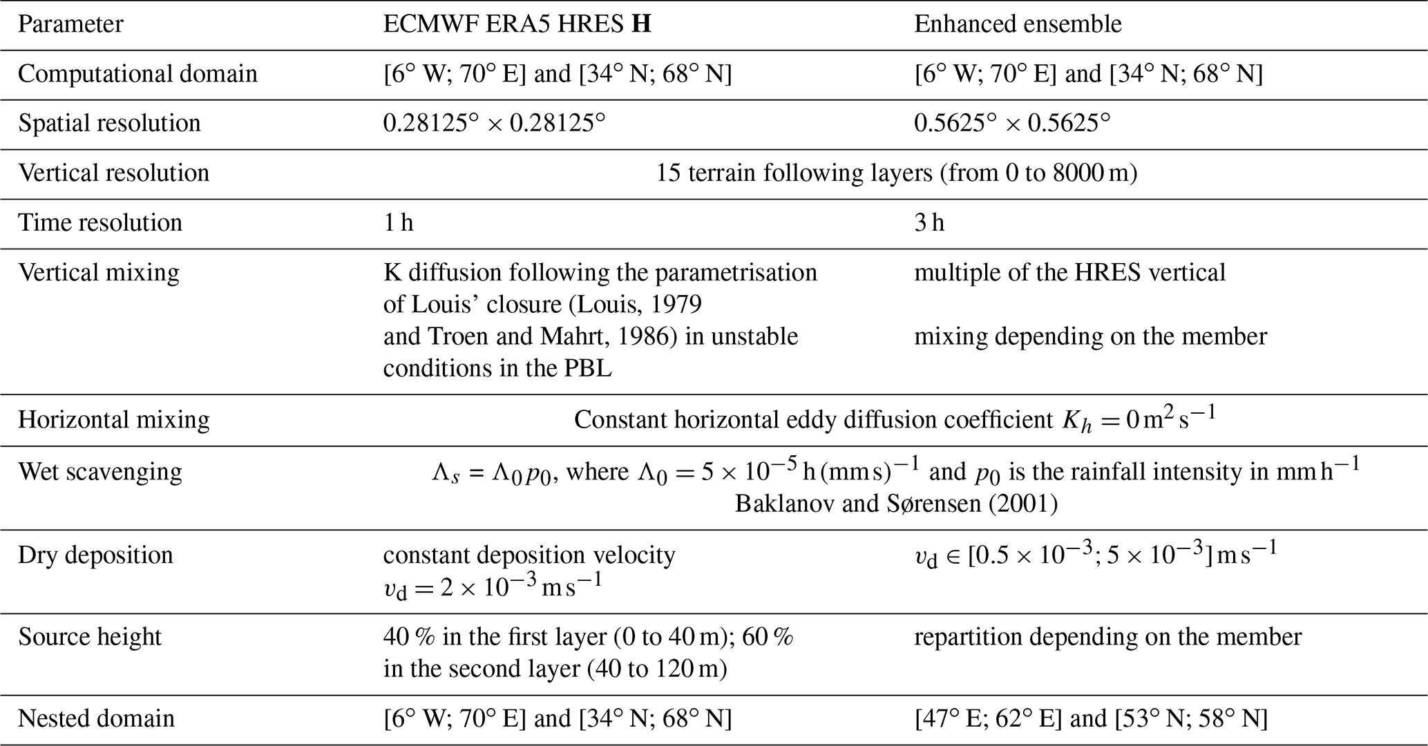
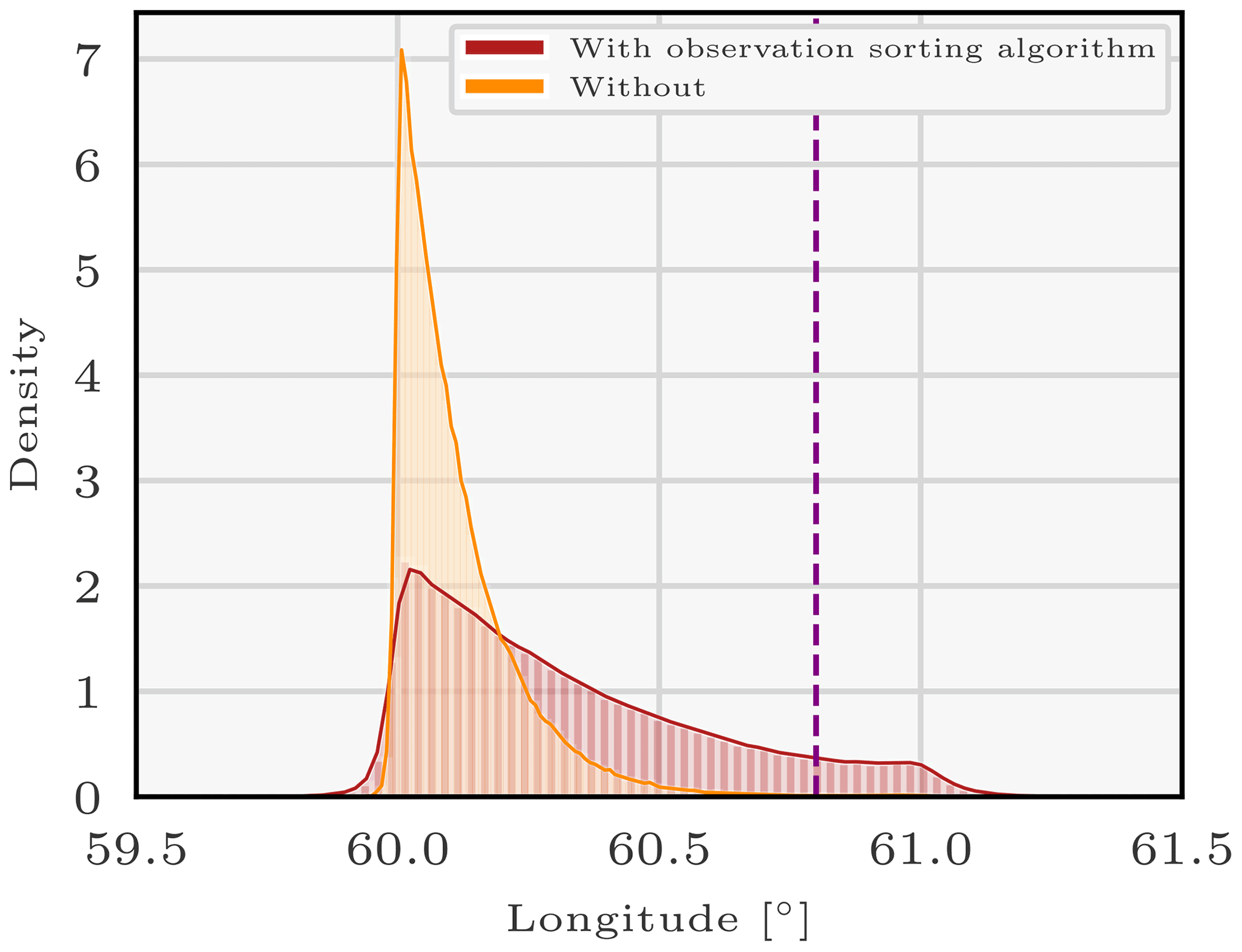
Figure 2 Density of the longitude for a log-Laplace likelihood with threshold 0.1 mBq m⁻³ of the ¹⁰⁶Ru source sampled with the 30 first members of the enhanced ensemble of observation operators using the parallel tempering method with or without the help of the observation-sorting algorithm. The purple vertical bar represents the longitude of the Mayak nuclear complex.

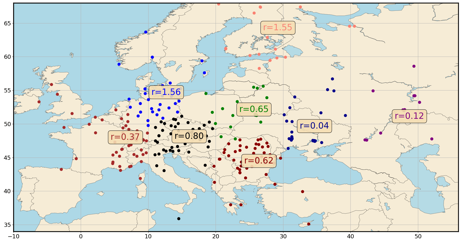
Figure 3 ¹⁰⁶Ru observations spatially clustered with a k means algorithm (k=9). The means of the corresponding nine variance distributions have been computed using a parallel tempering algorithm for a log-normal distribution with a threshold equal to 0.5 mBq m⁻³. The observation-sorting algorithm is applied and “eliminates” the low-uncertainty observations.

3 Airborne radioactivity increase in Europe in autumn 2017

3.1 Context

In this section, the methods are applied to the detection event of ¹⁰⁶Ru in Europe in autumn 2017. We first provide a brief context for the event and a review of earlier studies and describe the observation dataset and the model.

Small quantities of ¹⁰⁶Ru were measured by several European monitoring networks between the end of September and the beginning of October 2017. Inquiries to locate the source, the origin of the ¹⁰⁶Ru being unknown, have been carried out, based on the radionuclide measurements. Correlation methods are used by Kovalets et al. (2020) to retrieve the location of the source. Saunier et al. (2019) apply deterministic inverse modelling methods to reconstruct the most probable source and release: southern Ural is identified as the most likely geographical location, and the total release in the atmosphere is estimated to be 250 TBq. The location, release, and errors are also investigated by Dumont Le Brazidec et al. (2020), Tichý et al. (2021), and Western et al. (2020) using Bayesian methods. De Meutter et al. (2021) propose a methodology to retrieve the model error in the ¹⁰⁶Ru case.

The concentration measurements used in this study are available in Masson et al. (2019). The dataset has more than 1000 observations of ¹⁰⁶Ru with detection levels from a few µBq m⁻³ to more than 170 mBq m⁻³ in Romania. It is described in Fig. 1.

3.2 Modelling

3.2.1 Physical parametrisation

All simulations, described in Sect. 3.3, are driven using the ECMWF (European Centre for Medium-Range Weather Forecasts) ERA5 meteorological fields (Hersbach et al., 2020). A single observation operator H is built with the high-resolution forecast (HRES) reanalysis, in order to study the relevance of the methods presented in Sects. 2.1 and 2.2. An enhanced ensemble of 50 observation operators is built following the methodology of Sect. 2.3, where the ensemble of meteorological fields is the ERA5 EDA (Ensemble Data Assimilation) of 10 members. As explained in Sect. 2.3, each observation operator of this enhanced ensemble is the output of the transport model based on a random member of the ERA5 EDA and a random physical parametrisation. Table 1 refers to the parameters of the ldX dispersion simulations. The choice of parameters is based on the analysis carried out by Saunier et al. (2019) and Dumont Le Brazidec et al. (2020). As seen in Sect. 2.3 and Table 1, the vertical mixing of each member of the enhanced ensemble is a random multiple (between $\mathrm{1}/\mathrm{3}$ and 3) of the corresponding ECMWF EDA member vertical mixing. Furthermore, the constant dry deposition velocity and the distribution of the height of the release between the two first vertical layers of each member is unique and specific to this member. On most measurement stations, there was no rain event on the passage of the plume except for Scandinavia and Bulgaria. This suggests that wet deposition has a weak influence on the simulations, compared to the other processes.

Simulations are performed forward in time from 22 September 2017 at 00:00 UTC to 13 October 2017, which corresponds to the time of the last observation with resolutions defined in the Table 1. The HRES domain grid G of computation of the operators H corresponds to the nested domain of Table 1 and has been chosen based on previous works from the authors (Saunier et al., 2019; Dumont Le Brazidec et al., 2020). The enhanced ensemble domain grid where origin of the release is considered is of smaller extent due to computation power limitations and focuses on the most probable geographical domains of origin of the release, inferred from the HRES results presented in Sect. 3.3.3. The chosen mesh spatial resolution of G is 0.5^∘ for the simulations with the ECMWF ERA5 HRES observation operator and 1^∘ with the enhanced ensemble of observation operators. The logarithm of the release q is defined as a vector of size N_imp=9 daily release rates from 22 to 30 September, as explained in Dumont Le Brazidec et al. (2020). Therefore, ldX is run for each grid point of G and for each day between 22 and 30 September to build the observation operators.

3.2.2 Choice of the priors

In a Bayesian framework, the prior knowledge on the control variables for the ¹⁰⁶Ru source must be described. Following Dumont Le Brazidec et al. (2020), and because no prior information is available, longitude, latitude, observation error variance, and member weights prior probabilities are assumed to be uniform. Lower and upper bounds of the uniform distribution on the coordinates are defined by the nested domain of Table 1. The lower bound of the observation error variance is 0 and the upper bound is chosen as a very high and unrealistic value. Lower and upper bounds of members' weight probabilities are 0 and 1. The independent priors of the release rates are chosen as log-gamma distributions to prevent the values of the release increasing unrealistically: the scale term is chosen as e³⁰ and the shape parameter as 0 (Dumont Le Brazidec et al., 2020).

3.2.3 Parallel tempering algorithm

We rely on Markov chain Monte Carlo (MCMC) algorithms to sample from the target p(x|y). MCMC methods are asymptotically exact sampling methods not reliant on closed-form solutions. They are based on the use of Markov chains having as invariant distribution the posterior distribution of interest. A Markov chain is a stochastic model that describes a sequence of possible events that can converge to a distribution. Thus, after a sufficient time, the Markov chain samples values of this distribution. The convergence of a popular MCMC algorithm such as the Metropolis–Hastings (MH) algorithm can be hampered by the encounter of local minima and be delayed (Dumont Le Brazidec et al., 2020). To overcome this issue, the parallel tempering algorithm (Swendsen and Wang, 1986) is employed. Also called Metropolis-coupled Markov chain Monte Carlo (MCMCMC) or temperature swapping (Earl and Deem, 2005; Baragatti, 2011; Atchadé et al., 2011), it consists of combining several MCMC algorithms (such as MH) at different temperatures, where a temperature is a constant flattening out the posterior distribution. Chains with a flat target distribution avoids being trapped in local minima and provide probable source variable vectors to the “real” chain with no temperature. Details of the implementation applied to our problem can be found in Dumont Le Brazidec et al. (2020).

3.2.4 Parameters of the MCMC algorithm

The transition probabilities used for the random walk of the Markov chains are defined independently for each variable and based on the folded-normal distribution as described by Dumont Le Brazidec et al. (2020). The transition probability of the meteorological member weights is also defined as a folded-normal distribution. Weights are at first updated independently from each other, and then each proposal is updated by the sum of the weights, i.e.

$$\begin{array}{}\text{(8)}& \begin{array}{rl}& \forall i\in \mathit{\{}\mathrm{1},N_e\mathit{\}}{w}_i^k\sim \mathcal{F}\mathcal{N}(w_i^{k-\mathrm{1}},{\mathit{\sigma }}_w)\\ & \text{then }{w}_i^k={\displaystyle \frac{w_i^k}{{\sum }_{j=\mathrm{1}}^{N_e}{w}_j^k}},\end{array}\end{array}$$

where ℱ𝒩 is the folded-normal distribution, with σ_w the prior standard deviation of the weights and $w_i^{k-\mathrm{1}}$ the value of the weight of the member k before the walk.

The variances of the transition probabilities are chosen based on experimentations and are set to be ${\mathit{\sigma }}_{x_{\mathrm{1}}}={\mathit{\sigma }}_{x_{\mathrm{2}}}=\mathrm{0.3}{{}^{\circ }}^{\mathrm{2}}$, σ_ln q=0.03, σ_r=0.01, and σ_w=0.0005. All variables are always initialised randomly. Locations of the transition probabilities are the values of the variables at the current step. When the algorithm to discriminate observations presented in Sect. 2.2 is used, we consider that a prediction and an observation can be considered as equal if their difference is less than ϵ_d=0.1 mBq m⁻³, which is inferred from receptor detection limits described in Dumont Le Brazidec et al. (2020). Ten chains at temperatures t_i=cⁱ with c=1.5 are used in the parallel tempering algorithm.

3.3 Application of the methods

3.3.1 Overview

To see the impacts of the techniques proposed in Sect. 2 (i.e. using diverse likelihoods, new designs of the error covariance matrix, and an ensemble-based method), the pdfs of the variables describing the ¹⁰⁶Ru source are sampled from various configurations:

• Sect. 3.3.2 is an application of the observation-sorting algorithm presented in Sect. 2.2. It provides a comparison between the longitude pdf reconstructed with or without the observation-sorting algorithm to estimate its efficiency.

• Sect. 3.3.3 is an application of the use of different likelihood functions and strategies to spatially cluster observations in diverse groups. It presents results obtained using the HRES meteorology to analyse the impact of using several likelihood distributions. The observation-sorting algorithm is applied and two cases are explored: no spatial clustering of the observations, $\mathit{x}=(x_{\mathrm{1}},x_{\mathrm{2}},\ln \mathit{q},r_{\mathrm{1}},r_{\text{nd}})$, and spatial clustering of the observations with the corresponding modelling of the error covariance matrix R as described in the end of Sect. 2.2: $\mathit{x}=(x_{\mathrm{1}},x_{\mathrm{2}},\ln \mathit{q},r_{\mathrm{1}},\mathrm{\dots },r_k,r_{\text{nd}})$ where we use k=9.

• Sect. 3.3.4 is an application of the use of the ensemble-of-observation-operator strategy presented in Sect. 2.3. The enhanced ensemble with uncertainty on the dispersion parameters based on the ERA5 EDA of 10 members is analysed in Sect. 3.3.4. Afterwards, pdfs of the source variables x are sampled using the enhanced ensemble: $\mathit{x}=(x_{\mathrm{1}},x_{\mathrm{2}},\ln \mathit{q},r_{\mathrm{1}},r_{\text{nd}},w_{\mathrm{1}},\mathrm{\dots },w_{N_e})$. Results are reconstructed with the help of the observation-sorting algorithm and diverse likelihoods.

Note that, when the observation-sorting algorithm is used, in all cases, approximately half of the observations are sorted as non-discriminant.

3.3.2 Study of the interest of the observation-sorting algorithm

We present here an experiment supporting the observation-sorting method. A reconstruction of the source variables is proposed using the enhanced ensemble of observation operators, only on the first 30 members for the sake of computation time. The enhanced ensemble is studied later in Sect. 3.3.4. A log-Laplace likelihood with a threshold equal to 0.1 mBq m⁻³ is used in two cases: with or without applying the observation-sorting algorithm. The source variable vector is therefore ${\mathit{x}}_{\text{with}}=(x_{\mathrm{1}},x_{\mathrm{2}},\ln \mathit{q},r_{\mathrm{1}},r_{\text{nd}},w_{\mathrm{1}},\mathrm{\dots },w_{N_e})$ (with observation-sorting algorithm) or ${\mathit{x}}_{\text{without}}=(x_{\mathrm{1}},x_{\mathrm{2}},\ln \mathit{q},r,w_{\mathrm{1}},\mathrm{\dots },w_{N_e})$ (without).

Figure 2 represents the longitude variable pdf of the sources' variable vectors. The red histogram, which represents the longitude pdf in the case where the observation-sorting algorithm is applied, is far more spread out than the case without. It indeed ranges from 60 to 61.2^∘ while the orange longitude density (without applying the observation-sorting algorithm) ranges from 60 to 60.6; i.e. the pdf extent with sorting is the double of the spread without.

The mean of the observation error variance r samples in the case without the observation-sorting algorithm is 0.399. In the case with the observation-sorting algorithm, the discriminant observation error variance r₁ is equal to 0.63 and the non-discriminant observation error variance r_nd tends to a very low value. We denote x_with as the set of sources sampled (and therefore considered as probable) when using the observation-sorting algorithm and x_without as the set of sources sampled without. For example, a source x in x_with is of longitude x₁ in [60,61.2]. By definition of the log-Laplace pdf in Eq. (5), the fact that r_nd tends to a very low value confirms that non-discriminant observations are observations which are not able to discriminate between any of the sources in x_with.

What happens when the observation-sorting algorithm is not used (orange histogram), i.e. with the basic design R=rI, is that the observation error variance r is common for all observations. The resulting r=0.399 is therefore a compromise between r₁=0.63 and r_nd∼0, the variances sampled with the sorting algorithm. In other words, the uncertainty of the discriminant observations is reduced compared to the uncertainty found when applying the sorting algorithm. That is, the confidence in the discriminant observations is artificially high. This is why the extent of the resulting posterior pdfs is reduced compared to the case with the observation-sorting algorithm. More precisely, the probability of the most probable sources (here longitudes between 60 and 60.6) is increased and the probability of the least probable sources is decreased (longitudes between 60.6 and 61.2).

The observation-sorting algorithm is a clustering algorithm that avoids this compromise. Observations always equal to their predictions (i.e. associated with very small observation error variance, or with very high confidence for all probable sources) – the non discriminant observations – are assigned a specific observation error variable. In this way, the uncertainty variance associated with the other observations is far more appropriate. This clustering is totally valid as explained in Appendix B.

Finally, note that sampling the longitude posterior distribution using y_d the set of discriminant observations instead of y yields a pdf very similar to the red density in Fig. 2. In other words, considering observations which cannot discriminate between a source of longitude 60 and a source of longitude 60.8 actually decreases the probability of the source of longitude 60.8, which is not justifiable. The significant difference between the two pdfs makes the application of the algorithm necessary.

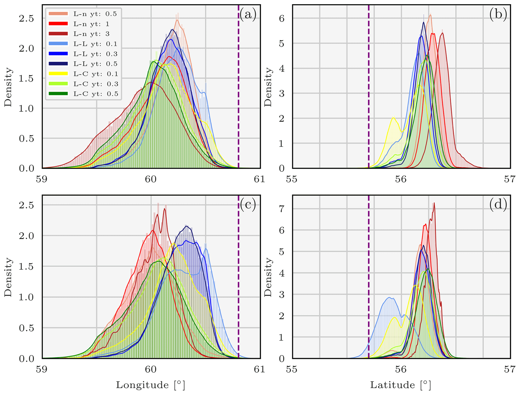
Figure 4 Pdfs of the coordinates describing the ¹⁰⁶Ru source sampled using the parallel tempering method and the observation-sorting algorithm and for various likelihoods in two scenarios: longitude without (a) and with observation spatial clustering in nine clusters (c) and latitude without (b) and with (d). L-L means log-Laplace, L-n means log-normal, L-C means log-Cauchy, and y_t is the likelihood threshold. The purple vertical bars represent the coordinates of the Mayak nuclear complex.

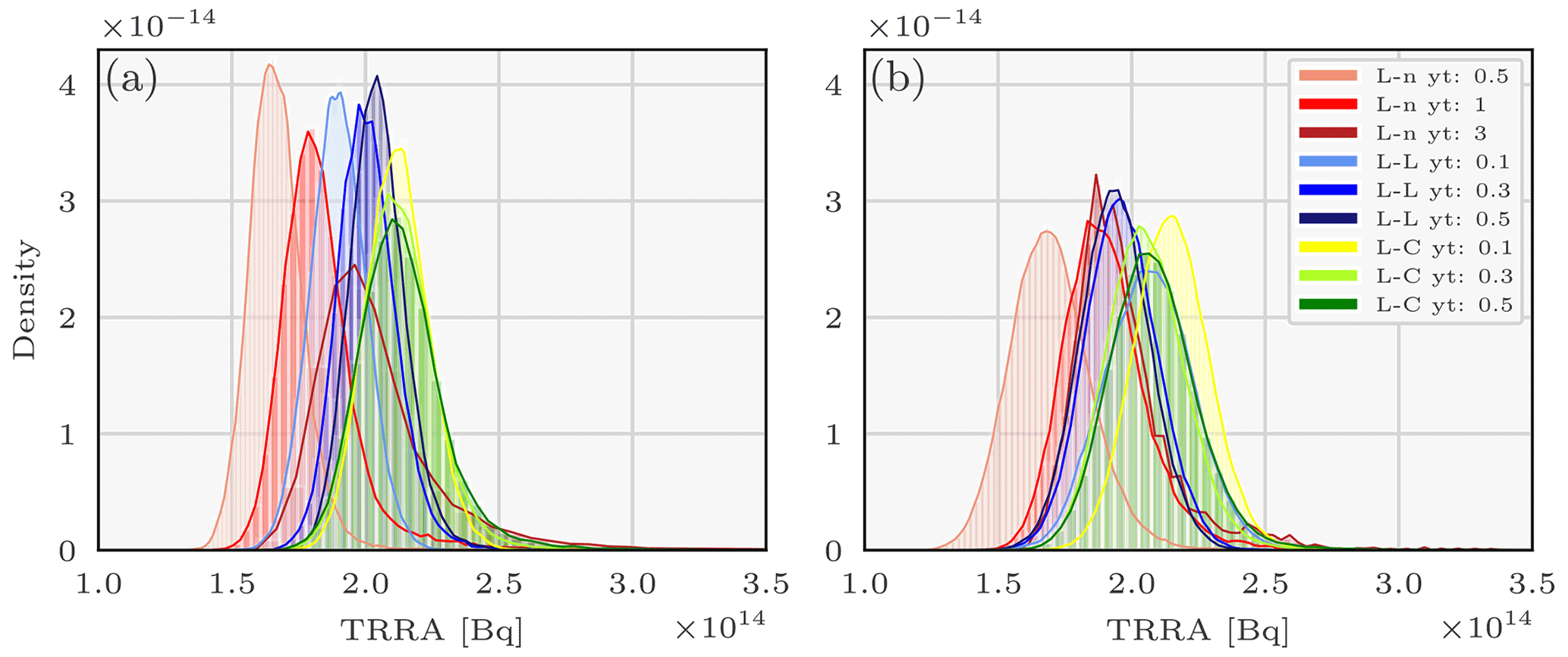
Figure 5 Pdfs of the total retrieved released activity (TRRA) describing the ¹⁰⁶Ru source sampled using the parallel tempering method and the observation-sorting algorithm and for various likelihoods in two scenarios: without (a) and with observation spatial clustering in nine clusters (b). L-L means log-Laplace, L-n means log-normal, L-C means log-Cauchy, and y_t is the likelihood threshold.

3.3.3 Sampling with the HRES data, several likelihoods, the observation-sorting algorithm, and with or without observation spatial clusters

In this section, we study two cases. First, we assess the impact of the choice of the likelihood on the reconstruction of the control variable pdfs ($\mathit{x}=(x_{\mathrm{1}},x_{\mathrm{2}},\ln \mathit{q},r_{\mathrm{1}},r_{\text{nd}})$), and second, we investigate how assigning diverse error variance terms to the observations according to a spatial clustering can affect the results ($\mathit{x}=(x_{\mathrm{1}},x_{\mathrm{2}},\ln \mathit{q},r_{\mathrm{1}},\mathrm{\dots },r_{\mathrm{9}},r_{\text{nd}})$). In this second case, clusters are computed with a k mean algorithm for k=9. Observation clusters are presented in the map below. As can be seen in Fig. 3, the nine variances sampled are diverse. We do not provide explanations of the values of these variances given that the observation-sorting algorithm is used and “eliminates” observations with low uncertainties. Therefore, the variances are only representative of observations with high uncertainties in their subset. However, the figure shows that the variances are very different: the use of a single parameter to represent them all is an important simplification. We now present the reconstruction of the pdfs in the two scenarios.

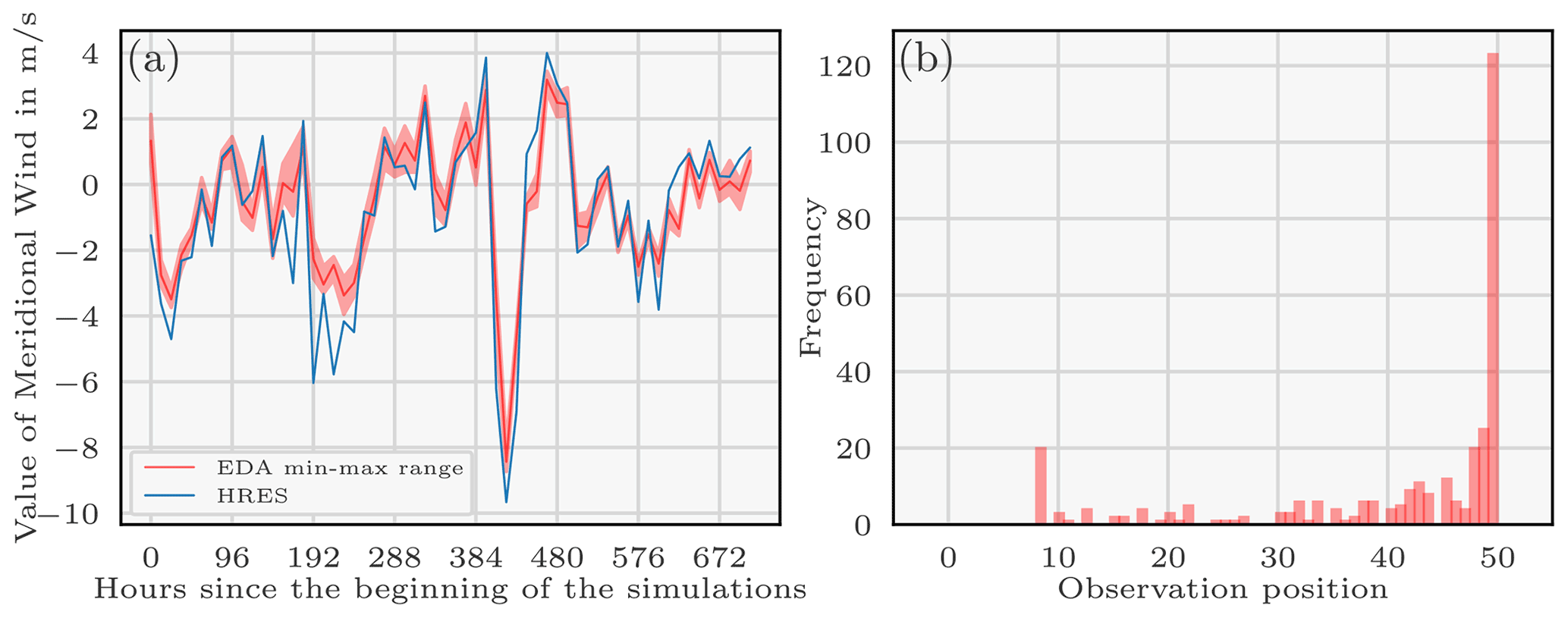
Figure 6 Evolution of the meridional wind of the HRES and EDA meteorologies for a random location in Europe since the beginning of the simulations. The red curve represents the mean of the meridional wind EDA members with the space between the minimum and maximum values (a). Rank histogram: comparison between the ¹⁰⁶Ru observations and the reference predictions of the enhanced ensemble (b).

Figures 4a, b and 5a show the marginal pdfs of the variables describing the source using the observation-sorting algorithm and for several likelihoods, using the HRES meteorology. The longitude pdf support ranges from 59 to 60.75^∘ E, and the latitude support from 55.75 to 56.75^∘ N. The extent of the joined coordinates pdfs is slightly greater than the extent of any coordinate pdf reconstructed using any likelihood distribution. Nevertheless, they are in general all consistent in the pointed area of ¹⁰⁶Ru release, especially given that the observation operators interpolation step is 0.5^∘.

The daily total retrieved released activity (TRRA) was mostly significant on 25 September. The extent of the release pdf overlap is smaller than the coordinates pdf overlap extent; probable TRRA values range from 140 to 300 TBq.

This shows that using a single likelihood is not enough to aggregate the whole uncertainty of the problem. Furthermore, we can see on these graphs that the threshold choice of the likelihood also has a moderate impact on the final coordinate pdfs and an important impact on the TRRA pdfs. More precisely, the daily TRRA pdfs obtained from the log-normal and the log-Laplace choices are moderately impacted by the threshold value choice.

Figures 4c, d and 5b show the marginal pdfs of the variables describing the source in the same configuration, except that nine error variances are used and assigned to the observations using the spatial clustering. The impact of this clustering is not significant: pdfs of the coordinates or the TRRA do not change meaningfully with the use of this representation of the R covariance matrix. Diverse trials for numbers of centroids between 3 and 9 have been carried out and all yield similar results.

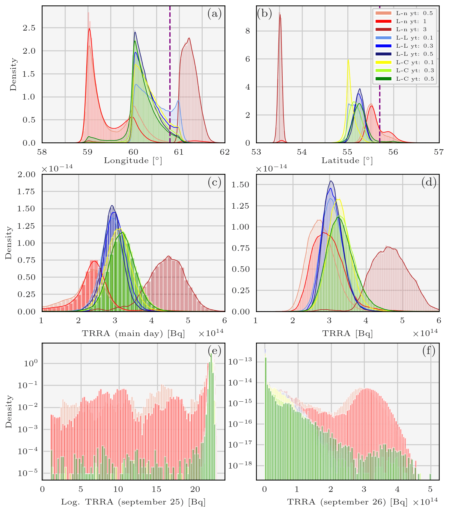
Figure 7 Pdfs of the variables describing the ¹⁰⁶Ru source sampled using the parallel tempering method and the enhanced ensemble of observation operators and the observation-sorting algorithm and for various likelihoods: longitude (a), latitude (b), TRRA on the main day (c), TRRA (d), log. TRRA on 25 September (e) and TRRA on 26 September (f). L-L means log-Laplace, L-n means log-normal, L-C means log-Cauchy, and y_t is the likelihood threshold.

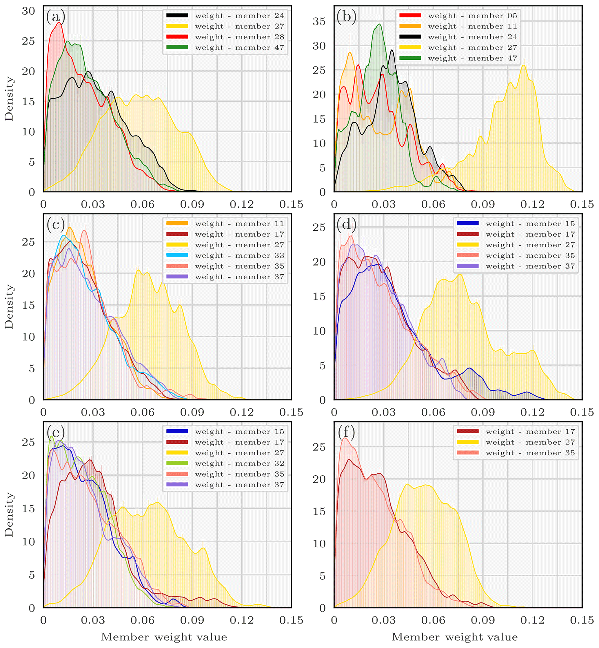
Figure 8 Densities of the weights of the members of the enhanced ensemble using the parallel tempering method and the observation-sorting algorithm for diverse likelihoods: log-normal with threshold 0.5 (a), log-normal with threshold 3 (b), log-Laplace with threshold 0.1 (c), log-Laplace with threshold 0.5 (d), log-Cauchy with threshold 0.1 (e), log-Cauchy with threshold 0.3 (f). L-L means log-Laplace, L-n means log-normal, L-C means log-Cauchy, and y_t is the likelihood threshold. Only densities with high medians are shown.

3.3.4 Sampling from the enhanced ensemble with weight interpolation

Before reconstructing the pdfs of the ¹⁰⁶Ru source using the observation operator ensemble, we study the dispersion of this enhanced ensemble, created by sampling on the transport model parameters and the ERA5 EDA. A number of 50 members are used to create the enhanced ensemble.

The original ERA5 EDA meteorology is under-dispersive as can be seen in Fig. 6a: in blue is drawn the HRES meridional wind predictions, and in red the EDA meridional wind mean prediction with the maximum and minimum values, for a random location in Europe. For most of the times, the ensemble values do not even recover the HRES value, which indicates that the ensemble has a small dispersion. ECMWF ensemble forecasts indeed tend to be under-dispersive in the boundary layer (especially in the short range) (Pinson and Hagedorn, 2011; Leadbetter et al., 2020). Furthermore, the release height parameter has low chances to be of significant impact. Therefore, with only two variables (Kz and dry deposition velocity) with high chances to be of significant impact to sample, we consider that 50 members is an adequate number.

To examine the spread of the ensemble of observation operators, we need to define a reference source x_ref for which predictions of the ensemble can be computed for each member and compared afterwards with the ¹⁰⁶Ru observations. Note that the reference source choice is necessarily an arbitrary choice which biases the results. We use the most probable source from Saunier et al. (2019) as the reference source: the reference source is located in [60,55] and with a release of 90 TBq on 25 September and of 166 TBq on 26 September. The corresponding rank diagram (Fig. 6b) shows that the predictions often underestimate the observation value. A ROC and a reliability diagram are provided in Appendix C to study more deeply the ensemble of observation operators.

We now study the impact of adding meteorological and transport uncertainties into the sampling process: $\mathit{x}=(x_{\mathrm{1}},x_{\mathrm{2}},\ln \mathit{q},r_{\mathrm{1}},r_{\text{nd}},w_{\mathrm{1}},\mathrm{\dots },w_{N_e})$. The integration of an enhanced ensemble to deal with the meteorological and dispersion uncertainties has a very interesting impact on the reconstruction of the source variables. In combination with the use of diverse likelihoods, pdfs of the longitude and latitude are significantly impacted as can be seen in Fig. 7a and b. The longitude pdf support ranges from 58.75 to 61.2^∘ E, and the latitude support ranges from 54.75 to 56.5^∘ N, not considering the results with the log-normal likelihood of threshold 3 mBq m⁻³. The “outlier” distribution reconstructed with the log-normal likelihood of threshold 3 mBq m⁻³ is indeed questionable, as it differs widely from all the others. The threshold of 3 mBq m⁻³ was chosen as an upper bound and does not seem to be the most appropriate choice. In Fig. 7d, the joint TRRA distribution (where joint means considering all likelihoods) ranges from 150–200 to 450–500 TBq, not considering the “outlier” reconstruction. The variance of the joint enhanced ensemble TRRA is therefore bigger than the variance of the joint HRES TRRA which ranged from 140 to 300 TBq. This means that the uncertainty emanating from meteorological data and the transport model is better quantified. Note also that with the log-normal likelihood and a threshold of 0.5 mBq m⁻³, or 1 mBq m⁻³, or log-Cauchy with a threshold of 0.3 or 0.5 mBq m⁻³, the release is split between the 25th and the 26th as can be noted in Fig. 7e and f. In other words, the integration of weights member interpolation adds uncertainty not only over the magnitude of the release but also over the timing of the release (here, the day).

The pdfs of the member weights are displayed in Fig. 8 for several likelihoods and thresholds. Only weight pdfs with high medians are included in the graphs for the sake of visibility. Member 27 is always included in the combination of weights which define the interpolated observation operator used to make the predictions and is often one of the most important or the most important part of this combination. Since the ERA5 EDA is not very dispersive, we can make the hypothesis that the weight density of a member mainly depends on the dispersion parameters which are used for creating this member (or observation operator). The height layer of the release for the operator member 27 is mainly the one between 40 and 120 m (>90 %), its deposition constant velocity is $\mathrm{0.6}\times {\mathrm{10}}^{-\mathrm{3}}\mathrm{m}{\mathrm{s}}^{-\mathrm{1}}$ which is very close to the lower bound (minimal possible deposit), and the Kz has been multiplied by 0.47. It also corresponds to member 6 of the ERA5 EDA.

Member 17 is present 4 times and corresponds to a deposition velocity of $\mathrm{1.2}\times {\mathrm{10}}^{-\mathrm{3}}\mathrm{m}{\mathrm{s}}^{-\mathrm{1}}$, a release mainly on the second layer (75 %), and a Kz multiplied by 1.32. Member 35 is present 4 times and corresponds to a deposition velocity of $\mathrm{3.3}\times {\mathrm{10}}^{-\mathrm{3}}\mathrm{m}{\mathrm{s}}^{-\mathrm{1}}$, a release mainly on the first layer (83 %), and a Kz multiplied by 0.45. Two hypotheses can be made: the weight of member 27 is large because it has a very small deposition velocity, and that deposition velocity is overestimated when using the standard choice. Second, Kz may be overestimated, since the members 27 and 35 are built out of a small multiplicator on the Kz.

These conclusions must, however, be largely qualified and are mainly proposed to present the interest and potential of the method.

4 Summary and conclusions

In this paper, we proposed several methods to quantify the uncertainties in the assessment of a radionuclide atmospheric source. In the first step, the impact of the choice of the likelihood which largely defines the a posteriori distribution when the chosen priors are non-informative was examined. Several likelihoods were selected from a list of criteria: log-normal, log-Laplace, and log-Cauchy distributions which quantify the fit between observations and predictions.

In the second step, we have focused on the likelihood covariance matrix R which measures the observation and modelling uncertainties. A method has been proposed to model this covariance matrix from a sorting of the observations into two groups, discriminant and non-discriminant, to avoid observations with low discrimination power to artificially decrease the spread of the posterior distributions.

Finally, in order to incorporate the uncertainties related to the meteorological fields and the transport model into the sampling process, ensemble methods have been implemented. An ensemble of observation operators, constructed from the ERA5 ECMWF EDA and a perturbation of the IRSN ldX transport model dry deposition, release height, and vertical turbulent diffusion coefficient parameters, was used in place of a deterministic observation operator. Following a Bayesian approach, each operator of the ensemble was given a weight which was sampled in the MCMC algorithm.

Thereafter, a full reconstruction of the variables describing the source of the ¹⁰⁶Ru in September 2017 and their uncertainty was provided, and the merits of these different methods have been demonstrated, improving each time the quantification of uncertainties.

First, the refinement of R according to the relevance criterion of the observations has been demonstrated following an application of parallel tempering. Due to the use of the sorting algorithm, the standard deviation of the density of the reconstructed longitude in a certain configuration was multiplied by two. In practice, the sorting algorithm avoids an underestimation of the observation error variance.

Second, independent MCMC samplings with the three likelihoods examined performed with the HRES meteorological fields showed that the support of the TRRA distribution was moderately impacted by the choice of the likelihood. This reveals that the uncertainties are not correctly estimated when using a single likelihood.

Finally, incorporating the uncertainties of the meteorological and transport fields using the observation operator set in combination with the use of multiple likelihoods had a significant impact on the conditional distribution of the TRRA, increasing the magnitude and timing of the release variances, but also on the conditional distribution of the release source coordinates. We have also shown that this method allows the reconstruction of transport model parameters such as dry deposition velocity or release height.

With the help of the three main methods proposed in this paper, the longitude spread of the ¹⁰⁶Ru source lies in between 59 and 61^∘ E, and the latitude spread between 55 and 56^∘ N. The total release is estimated to be between 200 and 450 TBq and peaked mainly on 25 September (although a release on 26 September cannot be neglected).

We recommend the use of all three methods when sampling sources of atmospheric releases: all three methods can have a moderate to large effect depending on the event modelling (e.g. the use of three likelihoods has a large effect only in combination with the inclusion of physical uncertainties). As far as the likelihood is concerned, we think that the log-Cauchy distribution is the most suitable while the choice of the associated threshold necessarily depends on the observations. We intend to apply the methods to the Fukushima–Daiichi accident.

Appendix A: False paradox of the discriminant and non-discriminant observations

Let us suppose that the cost function is computed from a Gaussian likelihood; then we have

$$\begin{array}{}\text{(A1)}& {\displaystyle }{\displaystyle }\mathcal{J}\left(\mathit{x}\right|\mathit{y})={\displaystyle \frac{\mathrm{1}}{\mathrm{2}}}\sum _{i=\mathrm{1}}^{N_{\text{obs}}}{\displaystyle \frac{(y_i-(\mathbf{H}\mathit{x}{)}_i{)}^{\mathrm{2}}}{r}}+{\displaystyle \frac{N_{\text{obs}}\ln \left(r\right)}{\mathrm{2}}}.\end{array}$$

Suppose we add to this set of observations y of size N_obs a second set of observations ${\mathit{y}}^{*}={\mathbf{0}}_{N_{\text{obs}}^{*}}$ of size $N_{\text{obs}}^{*}$ for which the corresponding predictions are also zero. This can happen for instance if we add observations preceding the accident.

If we take into account this new set of observations, the cost function becomes

$$\begin{array}{ll}{\displaystyle }\mathcal{J}\left(\mathit{x}\right|\mathit{y},{\mathit{y}}^{*})& {\displaystyle }={\displaystyle \frac{\mathrm{1}}{\mathrm{2}}}\sum _{i=\mathrm{1}}^{N_{\text{obs}}+N_{\text{obs}}^{*}}{\displaystyle \frac{(y_i-(\mathbf{H}\mathit{x}{)}_i{)}^{\mathrm{2}}}{r}}\\ {\displaystyle }& {\displaystyle }+{\displaystyle \frac{\mathrm{1}}{\mathrm{2}}}(N_{\text{obs}}+N_{\text{obs}}^{*})\ln \left(r\right)\\ \text{(A2)}& {\displaystyle }& {\displaystyle }={\displaystyle \frac{\mathrm{1}}{\mathrm{2}}}\sum _{i=\mathrm{1}}^{N_{\text{obs}}}{\displaystyle \frac{(y_i-(\mathbf{H}\mathit{x}{)}_i{)}^{\mathrm{2}}}{r}}+{\displaystyle \frac{\mathrm{1}}{\mathrm{2}}}(N_{\text{obs}}+N_{\text{obs}}^{*})\ln \left(r\right),\end{array}$$

since for each observation of the new set, $y_i=(\mathbf{H}\mathit{x}{)}_i=\mathrm{0}$. Suppose now that $N_{\text{obs}}^{*}$ goes to infinity; then the observation error variance r should tend to 0. As r→0, the distributions sampled are being more and more peaked.

Therefore in this configuration, adding a given number of observations anterior to the accident will degrade the distributions of the source variables. This problem is due to the homogeneous and hence inconsistent design of the observation error covariance matrix. Assigning a different r to this new set of observations would solve effectively this false paradox.

Appendix B: Study of the observation-sorting algorithm clustering with the Akaike information criterion (AIC)

We compare a first model (0) where only one variable r is used to describe the covariance matrix R and a second model (d) where two variables r₁ et r₂ are describing R with the AIC (Hastie et al., 2009). Therefore

$$\begin{array}{}\text{(B1)}& {\displaystyle }& {\displaystyle }\text{AIC}\left(\mathrm{0}\right)=\mathrm{2}-\mathrm{2}\ln \left(L\right(\mathrm{0}\left)\right),\text{(B2)}& {\displaystyle }& {\displaystyle }\text{AIC}\left(d\right)=\mathrm{4}-\mathrm{2}\ln \left(L\right(d\left)\right),\end{array}$$

where L(0) and L(d) are the maximum likelihoods when using the first and second model respectively. Using Gaussian likelihoods to facilitate calculations and out of normalisation constants,

$$\begin{array}{ll}\text{(B3)}& {\displaystyle \frac{\mathrm{1}}{\mathrm{2}}}\text{AIC}\left(\mathrm{0}\right)=& {\displaystyle }\mathrm{1}+{\displaystyle \frac{N}{\mathrm{2}}}\ln {\displaystyle \frac{S}{N}}+{\displaystyle \frac{N}{\mathrm{2}}},{\displaystyle \frac{\mathrm{1}}{\mathrm{2}}}\text{AIC}\left(d\right)=& {\displaystyle }\mathrm{2}+{\displaystyle \frac{N_{\mathrm{1}}}{\mathrm{2}}}\ln \left(r_{\mathrm{1}}\right)+{\displaystyle \frac{S_{\mathrm{1}}}{\mathrm{2}{r}_{\mathrm{1}}}}\\ \text{(B4)}& {\displaystyle }& {\displaystyle }+{\displaystyle \frac{N_{\mathrm{2}}}{\mathrm{2}}}\ln \left(r_{\mathrm{2}}\right)+{\displaystyle \frac{S_{\mathrm{2}}}{\mathrm{2}{r}_{\mathrm{2}}}},\end{array}$$

where $S_k={\sum }_{i=\mathrm{1}}^{N_k}{\left(y_i-(\mathbf{H}\mathit{x}{)}_i\right)}^{\mathrm{2}}$ and N₁ and N₂ are the number of observations assigned to the first and second model, respectively ($N_{\mathrm{1}}+N_{\mathrm{2}}=N_{\text{obs}}$). Therefore, comparing the max likelihoods of the two models,

$$\begin{array}{ll}{\displaystyle \frac{\mathrm{1}}{\mathrm{2}}}\left(\text{AIC}\left(\mathrm{0}\right)-\text{AIC}\left(d\right)\right)=& {\displaystyle }-\mathrm{1}+{\displaystyle \frac{N_{\mathrm{1}}}{\mathrm{2}}}\ln {\displaystyle \frac{(S_{\mathrm{1}}+S_{\mathrm{2}})N_{\mathrm{1}}}{(N_{\mathrm{1}}+N_{\mathrm{2}})S_{\mathrm{1}}}}\\ \text{(B5)}& {\displaystyle }& {\displaystyle }+{\displaystyle \frac{N_{\mathrm{2}}}{\mathrm{2}}}\ln {\displaystyle \frac{(S_{\mathrm{1}}+S_{\mathrm{2}})N_{\mathrm{2}}}{(N_{\mathrm{1}}+N_{\mathrm{2}})S_{\mathrm{2}}}}.\end{array}$$

We can note that the smaller S₂ (and therefore the bigger S₁), the better the model (d) compared to (0). The observation-sorting algorithm specifically aims at selecting a large set of observations (the non-discriminant observations y_nd) with a very small maximum likelihood S₂=S_nd.

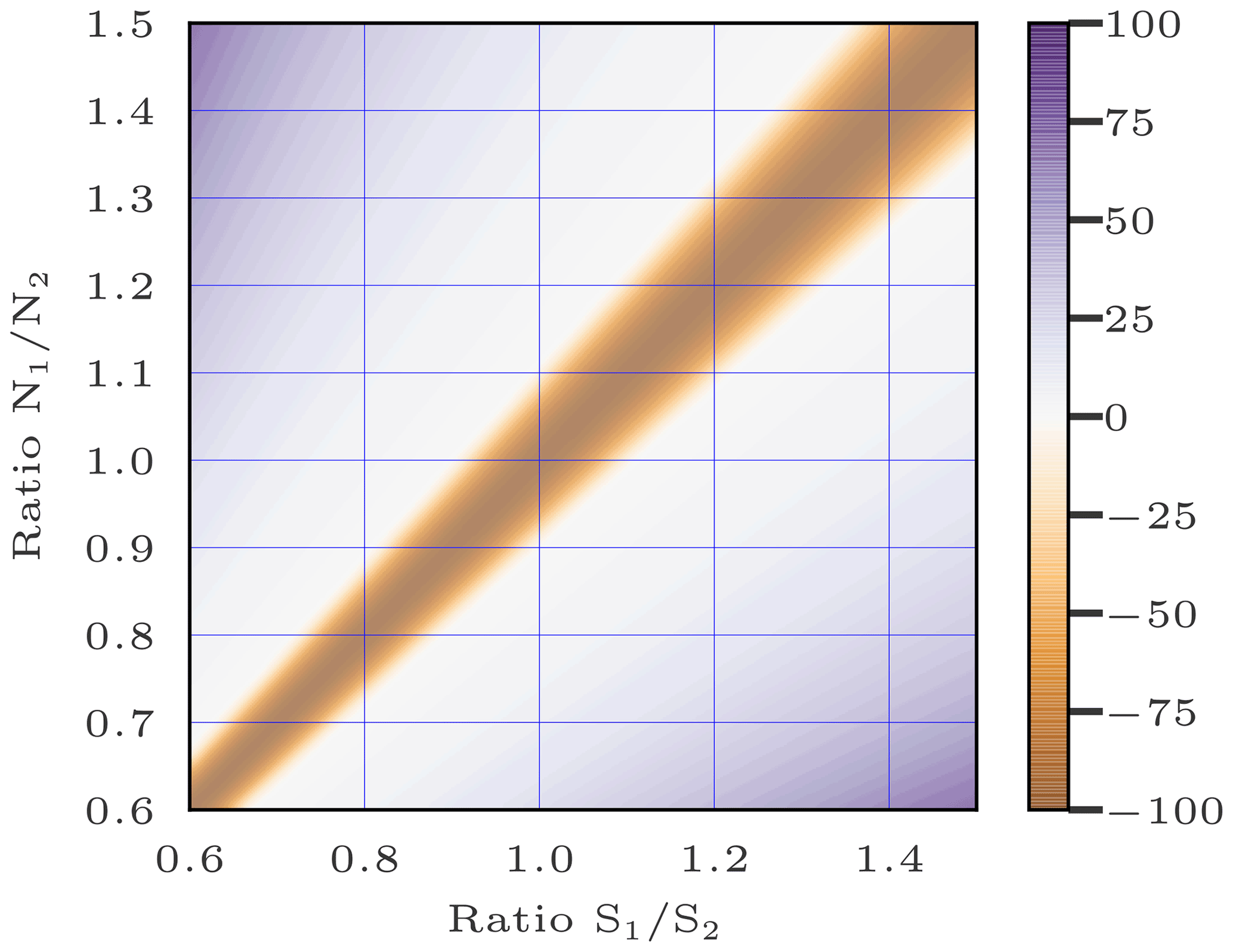
Figure B1 AIC(0) − AIC(d) with negative values multiplied by 100 to be more visible. Negative values indicate the cases where the model (0) with one variable is preferable. Positives values indicate the cases where the model (d) with two variables is preferable. On the x axis is the ratio between the likelihoods S₁ and S₂ linked to variables 1 and 2, respectively, of the model (d). On the y axis is the ratio between the numbers of observations N₁ and N₂ linked to variables 1 and 2, respectively, of the model (d).

We write $R=\frac{S_{\mathrm{1}}}{S_{\mathrm{2}}}$ and $M=\frac{N_{\mathrm{1}}}{N_{\mathrm{2}}}$ and use $N_{\mathrm{1}}+N_{\mathrm{2}}=N_{\text{obs}}$; then

$$\begin{array}{ll}{\displaystyle \frac{\mathrm{1}}{\mathrm{2}}}\left(\text{AIC}\left(\mathrm{0}\right)-\text{AIC}\left(d\right)\right)=& {\displaystyle }-\mathrm{1}+{\displaystyle \frac{N_{\text{obs}}M}{\mathrm{2}(\mathrm{1}+M)}}\ln \left({\displaystyle \frac{\mathrm{1}+\frac{\mathrm{1}}{R}}{\mathrm{1}+\frac{\mathrm{1}}{M}}}\right)\\ \text{(B6)}& {\displaystyle }& {\displaystyle }+{\displaystyle \frac{N_{\text{obs}}}{\mathrm{2}(\mathrm{1}+M)}}\ln \left({\displaystyle \frac{\mathrm{1}+R}{\mathrm{1}+M}}\right),\end{array}$$

and we can draw AIC(0) − AIC(d).

According to the AIC criterion, the model (d) with two variables is judged useless if the average likelihood of the observations y₁ linked to group 1 is close to the average likelihood of the observations y₂ linked to group 2. The observation-sorting algorithm specifically aims at creating two groups of observations: one where the average likelihood of the observations is close to 0 and another one where the average likelihood of the observations is high. In other words, the ratio ($S_{\mathrm{1}}/S_{\mathrm{2}}$) tends towards infinity (depending on the choice of ϵ_d) and the ratio ($N_{\mathrm{1}}/N_{\mathrm{2}}$), for example, is equal to 1. That is, the sorting algorithm creates two groups such that the corresponding coordinates ($S_{\mathrm{1}}/S_{\mathrm{2}}$) and ($N_{\mathrm{1}}/N_{\mathrm{2}}$) in Fig. B1 are as far away from negative values as possible. Therefore, the AIC criterion totally justifies the need for the clustering accomplished by the observation-sorting algorithm.

Appendix C: ROC and reliability diagram of the observation operators ensemble

A ROC and a reliability diagram are computed using the reference source defined in Sect. 3.3.4 to assess the ability of the forecast to discriminate between events and non-events and its reliability, respectively (Delle Monache et al., 2006). A good ROC curve is as close as possible to 1 in probability of a hit and to 0 in probability of a false occurrence. We recall that a hit for a certain threshold t is when the observation belongs to the considered interval and a number of corresponding predictions greater than the threshold t belong to the considered interval. A false occurrence is when the observation does not belong to the considered interval but a number of corresponding predictions greater than the threshold t belong to the considered interval. The ROC is plotted for a list of thresholds t.

Each curve of Fig. C1a and b corresponds to a dichotomous event: $y\in [y_{\text{min}};y_{\text{max}}]$ where y is an observation, and y_min and y_max are the values that define whether the event is true or false for y. These indicators are plotted for several ranges [y_min,y_max]. A reliable ensemble, for a given event, has a reliability curve as close as possible to the identity function.

From the ROC curves, the enhanced ensemble appears to be good for discriminating: curves always have a low rate of false occurrence and an acceptable hit rate. In the reliability diagrams, the forecast overestimates the probability that an observation is between 0 and 20 mBq m⁻³ which relates to predictions underestimating the observations in general. For the three other events, the diagrams show an acceptable reliability in the enhanced forecast.

Figure C1 ROC curve and reliability diagram of the enhanced ensemble created with sampling of EDA and the transport model parameters.