the Creative Commons Attribution 4.0 License.
the Creative Commons Attribution 4.0 License.
 | 06 Sep 2021
Forecasting and identifying the meteorological and hydrological conditions favoring the occurrence of severe hazes in Beijing and Shanghai using deep learning
Severe haze or low-visibility events caused by abundant atmospheric aerosols have become a serious environmental issue in many countries. A framework based on deep convolutional neural networks containing more than 20 million parameters called HazeNet has been developed to forecast the occurrence of such events in two Asian megacities: Beijing and Shanghai. Trained using time-sequential regional maps of up to 16 meteorological and hydrological variables alongside surface visibility data over the past 41 years, the machine has achieved a good overall performance in identifying haze versus non-haze events, and thus their respective favorable meteorological and hydrological conditions, with a validation accuracy of 80 % in both the Beijing and Shanghai cases, exceeding the frequency of non-haze events or no-skill forecasting accuracy, and an F1 score specifically for haze events of nearly 0.5. Its performance is clearly better during months with high haze frequency, i.e., all months except dusty April and May in Beijing and from late autumn through all of winter in Shanghai. Certain valuable knowledge has also obtained from the training, such as the sensitivity of the machine's performance to the spatial scale of feature patterns, that could benefit future applications using meteorological and hydrological data. Furthermore, an unsupervised cluster analysis using features with a greatly reduced dimensionality produced by the trained HazeNet has, arguably for the first time, successfully categorized typical regional meteorological–hydrological regimes alongside local quantities associated with haze and non-haze events in the two targeted cities, providing substantial insights to advance our understandings of this environmental extreme. Interesting similarities in associated weather and hydrological regimes between haze and false alarm clusters or differences between haze and missing forecasting clusters have also been revealed, implying that factors, such as energy-consumption variation and long-range aerosol transport, could also influence the occurrence of hazes, even under unfavorable weather conditions.
- Article
(17212 KB) - Full-text XML
-
Supplement
(6501 KB) - BibTeX
- EndNote


Frequent low-visibility or haze events caused by elevated abundance of atmospheric aerosols due to fossil fuel and biomass burning have become a serious environmental issue in many Asian countries in recent decades, interrupting economic and societal activities and causing human health issues (e.g., Chan and Yao, 2008; Silva et al., 2013; Lee et al., 2017). For example, rapid economic development and urbanization in China have caused various pollution-related health issues, particularly in populated metropolitan area such as the Beijing–Tianjin region and Yangtze River delta centered in Shanghai (e.g., Liu et al., 2017). In Singapore, the total economic cost caused by severe hazes in 2015 is estimated to be USD 510 million (0.17 % of the GDP) or USD 643.5 million based on a wiling-to-pay analysis (Lin et al., 2016). To ultimately prevent this detrimental environmental extreme from happening requires rigid emission control measures in place through significant changes in energy consumption and land and plantation management. Before all of these measures can finally take place, it would be more practical to develop skills to accurately predict the occurrence of hazes to allow for mitigation measures to be implemented ahead of time.
Severe haze events arise from the solar radiation extinction by aerosols in the atmosphere; this mechanism can be enhanced with the increase of relative humidity that enlarges the size of particles (e.g., Kiehl and Briegleb, 1993). Aerosols also need favorable atmospheric transport and mixing conditions to reach places away from their immediate source locations, while their lifetime in the atmosphere can be significantly reduced by rainfall removal. In addition, soil moisture is also a key to dust emissions. Therefore, meteorological and hydrological conditions are critical to the occurrence of haze events in addition to particulate emissions. To forecast the occurrence of such events using existing atmospheric numerical models developed based on fluid dynamics and explicit or parameterized representations of physical and chemical processes, first it is required for the models to accurately predict the concentration of aerosols at a given geographic location and a given time in order to correctly derive surface visibility (e.g., Lee et al., 2017, 2018). However, the propagation of numerical or parameterization errors through the model integration could easily drift the model away from the original track, not to mention that a lack of real-time emission data alone would also handicap such an attempt. Therefore, a more fundamental issue in practice is whether these models could reproduce the a posteriori distribution of the possible outcomes of the targeted low-probability extreme events. Ultimately, lack of knowledge about the extreme events would, in turn, hinder the effort to improve the forecasting skills.
Differing from the deterministic models, an alternative statistical prediction approach could be adopted if the predictors of a targeted event could be identified and a statistical correlation between them could be established with confidence. However, this is a rather difficult task for the traditional approaches, because it requires an analysis dealing with a very large quantity of high-dimensional data to establish and generalize a likely multi-variate and nonlinear correlation. Nevertheless, such attempts can obviously benefit now from the fast-growing sectors of machine learning (ML) and deep-learning (DL) algorithm development (e.g., LeCun et al., 2015). In addition, technological advancement and continuous investment from governments and other sectors across the world have led to a rapid increase in quantity and substantially improved quality of meteorological, oceanic, hydrological, land, and atmospheric composition data. These data might still not be sufficient for evaluating and improving certain detailed aspects of the deterministic forecasting models. However, rich information contained in these data about favored environmental conditions for the occurrence of extreme events such as hazes could already have great value for developing alternative forecasting skills.
Many Earth science applications dealing with meteorological or hydrological data need a trained machine not only to forecast values but also to recognize patterns or images. However, this can easily lead to a curse of dimensionality for many traditional ML algorithms. Fortunately, deep learning that directly links a large quantity of raw data with targeted outcomes through deep convolutional neural networks (CNNs) (Goodfellow et al., 2016) offers a clear advantage in sufficiently training deep networks suitable for solving highly nonlinear issues. In doing so, DL can also eliminate the possible mistakes in data derivation or selection introduced by subjective human opinion regarding a poorly understood phenomenon. Recently, DL algorithms have been explored in various applications in atmospheric, climate, and environmental sciences, ranging from recognizing specific weather patterns (e.g., Liu et al., 2016; Kurth et al., 2018; Lagerquist et al., 2019; Chattopadhyay et al., 2020), weather forecasting, including hailstorm detection (e.g., Grover et al., 2016; Shi et al., 2015; Gagne et al., 2019), deriving model parameterizations (e.g., Jiang et al., 2018), and beyond.
In certain applications, the targeted outcomes are the same features as the input but at a different time, e.g., a given weather feature(s) such as temperature or pressure at a given level. The forecasting can thus proceed by using pattern-to-pattern correlation from a sequential training dataset with spatial information preserving full CNNs such as U-net (Ronneberger et al., 2015; Weyn et al., 2020). However, this is certainly not the case for the applications where the environmental conditions associated with the targeted outcome are yet known. For such applications, a possible solution is to utilize a large quantity of raw data with minimized human intervention in data selection to train a deep CNN to associate targeted outcomes with favored environmental conditions. This study represents such an attempt, where a DL forecast framework is trained to identify the meteorological and hydrological conditions associated with the occurrences of severe hazes. The DL framework has been developed to be initially targeted at the severe hazes in Singapore (Wang, 2020) and now hazes in two megacities of China, Beijing and Shanghai. In terms of particulate pollutant emissions, all of these cities share certain sources, including fossil fuel combustion from transportation, domestic, and industries. On the other hand, each city also has its own unique sources, for instance, desert and perhaps anthropogenic dust for Beijing and massive biomass burning in Singapore (Liu et al., 2017; Lee et al., 2017, 2018, 2019). It is obvious that in addition to meteorological and hydrological conditions, dynamical patterns of anthropogenic activities leading to the emissions of particulate matters are also important factors behind the occurrence of severe hazes. Nevertheless, the major purpose of this study is to advance our fundamental knowledge about the weather conditions favoring the occurrence of hazes and, through an in-depth analysis on the forecasting results, to identify the limit of such a machine and thus to provide useful information for establishing a more complete forecasting platform for the task.
In the paper, the architecture involved, as well as the method and data used for training, are described after this introduction, followed by a discussion of training and validation results. Following this, an unsupervised cluster analysis that benefited from the trained machine is introduced along with its results, which further the understanding of the CNN's performance and summarize, for the first time, the various typical meteorological and hydrological regimes associated with haze versus non-haze situations in the two cities. The last section concludes the effort and provides its major findings.
2.1 Network architecture
The convolutional neural network used in this study, the HazeNet (Wang, 2020), has been developed by adopting the general architecture of the CNN developed by the Oxford University's Visual Geometry Group (VGG-Net) (Simonyan and Zisserman, 2015). The actual structure and hyper-parameters of HazeNet have been adjusted and fine-tuned based on numerous test training runs. In addition, certain techniques that were not available when the original VGG net was developed, e.g., batch normalization (Ioffe and Szegedy, 2015), have been included as well. The current version for haze applications of Beijing and Shanghai, though trained separately, contains the same number of parameters, 20 507 161 (11 376 non-trainable), owing to it having the same optimized kernel sizes. Figure 1 shows the general architecture of a HazeNet version with 12 convolutional and 4 dense layers (in total 57 layers).
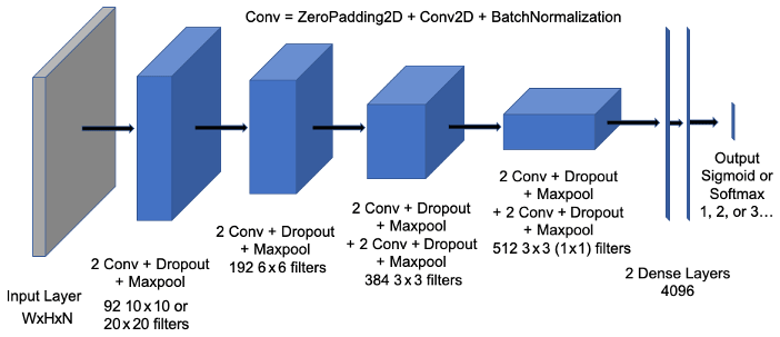
Figure 1Architecture of the 12 convolutional plus 4 dense layers of HazeNet. Here “Conv” represents a unit containing zero padding and then a 2D convolutional layer, followed by a batch normalization layer. There is a flattened layer before the two dense layers. W stands for width, H stands for height, and N stands for the number of features of the input fields (i.e., 64, 96, and 16 for Beijing and 64, 64, and 16 for Shanghai.
The network has been trained in a standard supervised learning procedure for classification, where the network takes input features to produce classification output that are then compared with known results or labels based on observations. The coefficients of the network are thereafter optimized in order to minimize the error between the prediction and the observation or label. The loss function used in optimization is cross-entropy (e.g., Goodfellow et al., 2017). Such a procedure is repeated until the performance of the network can no longer be improved. In practice, the training usually lasts about 2000 epochs (each epoch is a training cycle that uses up the entire training dataset). This procedure is intended to train a deep CNN to recognize and then associate input features (bundled meteorological and hydrological conditions in this case) with a corresponding class, i.e., severe haze events or non-haze events. As a result, the specific knowledge about the favored meteorological and hydrological conditions of severe hazes can thus be advanced.
2.2 Training data and methodology
The labels for the training are derived using the observed daily surface visibility (hereafter referred to as “VIS”) obtained from the Global Surface Summary Of the Day (GSOD) dataset consisting of daily observations of meteorological conditions from tens of thousands of airports around the globe (Smith et al., 2011). In the cases of Beijing and Shanghai, data are from observations in the corresponding airports of these two cities during the time from 1979 to 2019, containing 14 975 samples. For simplicity, the discussions will be mainly about the two-class training, where events with VIS ≤ the long-term mean value of the 25th percentile or p25 of VIS (6.27 km in Beijing, 5.95 km in Shanghai; Fig. 2b; see also Fig. S1 in the Supplement) are defined as class 1 or severe haze and events are otherwise classified as class 0 or non-haze cases. Although p25 values vary interannually, their long-term means represent a substantial reduction of VIS due to high particulate pollution (e.g., Lee et al., 2017). Note that unlike in the case of Singapore (Wang, 2020), fog and mist are more common low-visibility events in Beijing and Shanghai and thus have been excluded from the labels of severe hazes by following GSOD fog marks. The number of severe haze events that occurred during 1979–2019 defined in the above procedure is 3099 and 2999 for Beijing and Shanghai, indicating a frequency of 20.7 % and 20.0 %, respectively.
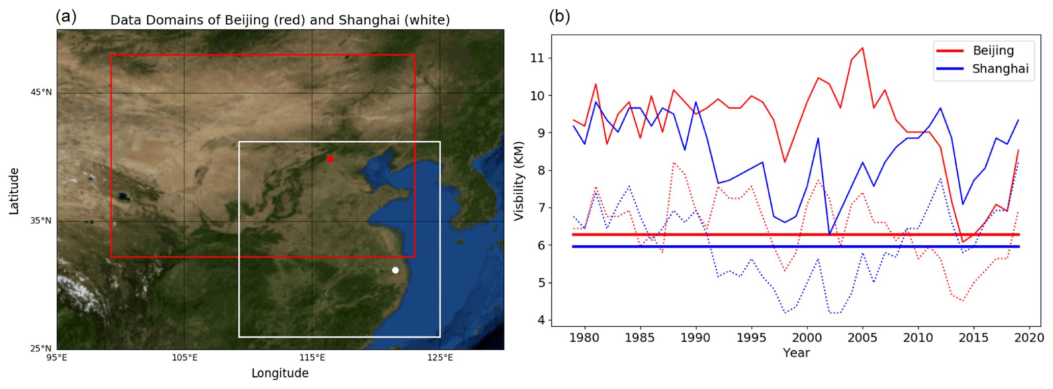
Figure 2(a) The input feature defining domains for Beijing (red box and dot, 32.25–48∘ N, 99.25–123∘ E; 64×96 grids with ERA5 data) and Shanghai (white box and dot, 26–41.25∘ N, 109.25–125∘ E; 64×64 grids), made using the Basemap library (a Matplotlib extension). (b) Annual means (solid curves), 25th percentiles (dashed curves), and 25th percentile means (solid straight lines) of surface visibility in Beijing (red) and Shanghai (blue) between 1979 and 2019.
The training and validation of HazeNet also need the input features with the same sample dimension of the labels. These input data are derived from hourly maps of meteorological and hydrological variables covering the data collection domain (Fig. 2a), obtained from ERA5 reanalysis data produced by the European Centre for Medium-range Weather Forecasts or ECMWF (Hersbach et al., 2020). These data are distributed in a grid system with a horizontal spatial interval of 0.25∘. Up to 16 features are derived from the original hourly data fields covering the analysis domain for Beijing (64×96 grids) and Shanghai (64×64 grids), including daily mean of surface relative humidity (REL), daytime change and daily standard deviation of 2 m temperature (DT2M and T2MS, respectively), daily mean of 10 m zonal and meridional wind speed (U10 and V10, respectively), daily mean of total column water (TCW), daily mean (TCV) and daytime change (DTCV) of total column water vapor, daily mean of planetary boundary layer height (BLH), daily mean soil water volume in soil layer 1 and 2 (SW1 and SW2, respectively), daily mean of total cloud cover (TCC), daily mean geopotential heights at 500 (Z500) and 850 (Z850) hPa pressure levels and their daytime changes (D500 and D850, respectively). All input features have been normalized into a range of [−1, +1] (Fig. S2 in the Supplement).
Before the training, the entire samples of labels alongside corresponding input features were randomly shuffled first then split in the following way: two-thirds of the samples went to the training set, and one-third of the samples went to the validation set, each is duly used for its designated purpose throughout the entire training process without switching. The above procedure treats each event as an independent sample. For the convenience of being able to compare performance or restart training based on a saved machine, a saved training dataset and a holdout validation dataset that has never been used in training were produced following the above procedure and used for the purpose.
The number of samples used in training HazeNet is rather limited compared to deep-learning standards. However, to associate 16 joint two-dimensional maps with targeted labels even with the current number of samples is still a demanding task that requires a deep CCN to accomplish. Furthermore, the targeted severe hazes are low-probability events. Their frequency of appearance is about 20 % in the Beijing and Shanghai cases. Therefore, a trained machine would easily bias toward the overwhelming non-haze events. To resolve these issues, a combination of class weight and batch normalization has been implemented in HazeNet, which both use corresponding Keras functions. The class weight is used to change the weight of training loss of each class, normally by increasing the weight of the low-frequency class. The class weight coefficient was calculated based on the ratio of class 0 to class 1 frequency. Batch normalization (Ioffe and Szegedy, 2015) is an algorithm to renormalize the input distribution at certain step (e.g., for each mini batch) to eliminate the shift of such distributions during optimization. The above approaches have effectively reduced the overfitting while overcoming the data imbalance issue, making the long training of a deep CNN possible (Wang, 2020). Entire training events have been conducted using a NVIDIA Tesla V100-SXM2 GPU cluster, costing 25 and 17 s per epoch for the machines in Beijing and Shanghai, respectively.
2.3 Kernel size optimization
As in the cases of other CNNs, there are many hyperparameters of HazeNet that need to be determined or optimized. These have been done through numerous testing training events. In practice, the deep architecture of HazeNet and the long training procedure have actually made the performance less sensitive to many hyperparameters of the network. One hyperparameter, however, is specifically interesting to explore in its application using a large quantity of meteorological maps, i.e., the kernel size of the first convolutional layer, where the input data (meteorological and hydrological maps) are convoluted and then propagated into the subsequent layers.
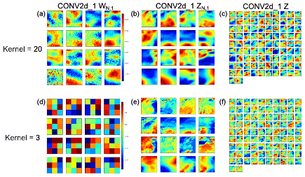
Figure 3(a, d) Weight coefficients of the first filter set (WN,1), (b, e) partial output for each feature (ZN,1), and (c, f) the output (Z) of the first convolution layer (CONV2d_1) with two selected kernel sizes (ks): (a–c) 20×20 and (d–f) 3×3. Here W represents the filters and Z the output of convolution; the subsets of Z before the feature dimension is merged can be expressed as , with the order of input features N=1, … 16 and i representing the convolutional layer index, i.e., 1 is the first layer or CONV2d_1. For the first layer, input feature size is , the set of filters is 92, and thus the final output Z has a dimension of (, , 92). Shown are the results from the training for Shanghai haze cases.
Meteorological maps or images often contain characteristic patterns with different spatial scales. Intuitively, preserving these patterns could be important in predicting the targeted extremes. Apparently, a larger kernel size produces smoother output images from the first convolutional layer, while a smaller kernel size can preserve many spatial details of the meteorological maps, as demonstrated by the layer output shown in Fig. 3. In practice, however, the patterns produced by the latter configuration might be too complicated for the networks to recognize and to perform classification, whereas patterns resulting from a relatively larger kernel size for the first convolutional layer might be more suitable for the task. The actual result suggests that HazeNet configured with a first-layer kernel size of 20 to 26 or close to 5–6∘ in spatial resolution consistently produces a better performance (about a 10 % improvement in F1 score) than that using a smaller kernel size of 3 or 6. As a result, a kernel size of 20 has been adopted as the default configuration for the first two convolutional layers in this study.
Currently, it is still difficult to find any practical score for forecasting the occurrence of severe hazes for comparison. Therefore, the performance of HazeNet has mainly been measured by using certain commonly adopted metrics for classification that are largely derived from the concept of the so-called confusion matrix (e.g., Swets, 1988; Table A1), including accuracy, precision, recall, F1 score, equitable threat score (ETS), and Heidke skill score (HSS) (Appendix A). Unless otherwise indicated, the discussions on the performance scores are hereafter referring to the severe haze class (or class 1) and are obtained from validation rather than training. In all the cases, the performance metrics referring to non-haze or class 0 have much better scores. Also note that, unless otherwise indicated, results shown in this Section are obtained using 16 features.
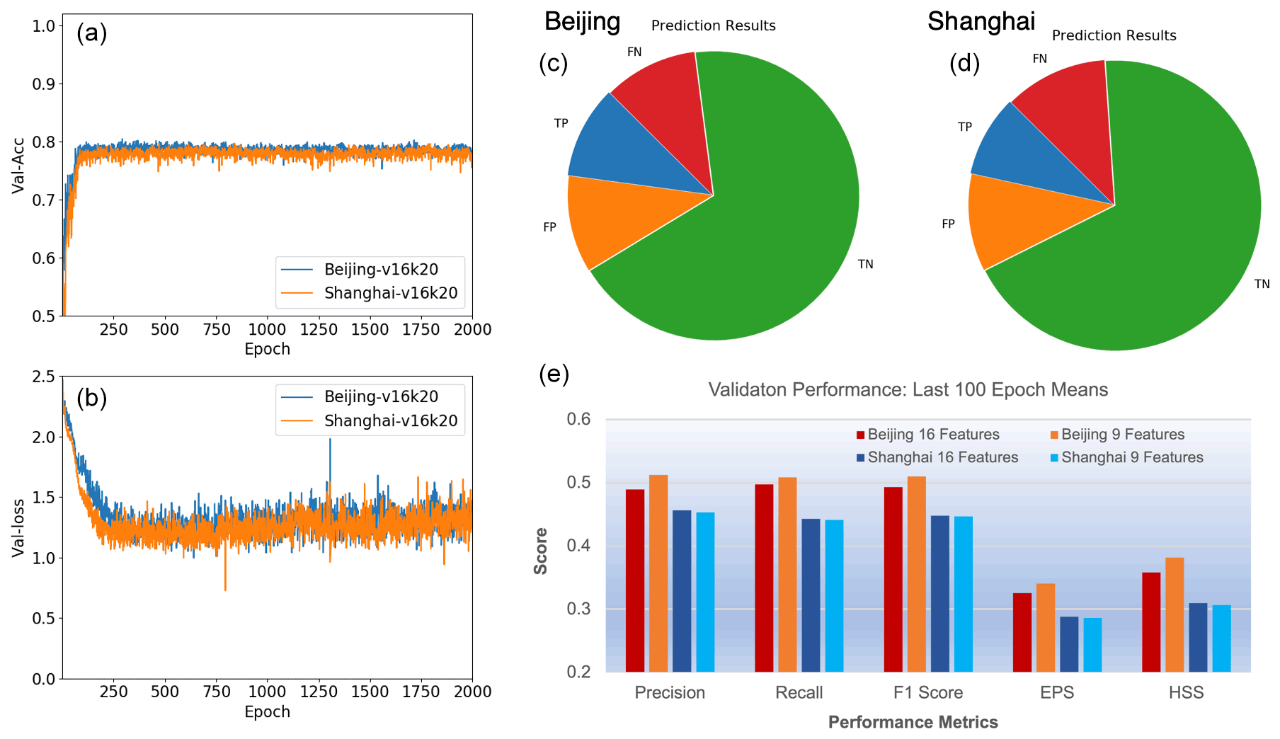
Figure 4(a, b) Validation accuracy (a) and loss (b) of HazeNet with 16 features for the Beijing and Shanghai cases; kernel size for the first filter is 20×20. (c, d) Prediction outcomes in reference to haze events (or class 1) of Beijing and Shanghai with 16 features. TP stands for true positive, TN stands for true negative, FP stands for false positive, and FN stands for false negative prediction outcomes. (e) Scores of performance metrics shown as means over the last 100 epochs for Beijing and Shanghai with 16 and 9 features, respectively.
In order to train a stable machine, training events with 2000 epochs or longer have been conducted instead of using certain commonly adopted skills such as early stop. As a result, the validation performance metrics of the trained machines all appeared to be stabilized by approaching the end of training (Fig. 4). These scores were consistent with the results of ensemble training with the same configuration but different randomly selected training and validation datasets and were also comparable among training events with different configurations. Overfitting has been clearly overcome due to such a long training procedure and the adoption of class weight and batch normalization. In a two-class classification (haze versus non-haze), trained deep HazeNet can always reach an almost perfect training accuracy (e.g., 0.9956 for Beijing cases) and a validation accuracy of 80 % (frequency of non-haze events or no-skill forecasting accuracy) in both Beijing and Shanghai cases (Fig. 4a). At the same time, the performance scores for predicting specifically severe hazes are also very reasonable, e.g., for Beijing cases either precision or recall exceeds 0.5 (they normally evolve in opposite directions), leading to a nearly 0.5 F1 score (Fig. 4c–e). The corresponding scores in training are obviously much higher, e.g., with precision, recall, and F1 as 0.9804, 0.9980, and 0.9880, respectively for Beijing cases, owing to the deep and thus powerful CNNs. HazeNet performed slightly better than several known deep CNNs, such as Inception Net V3 (Szegedy et al., 2015), ResNet50 (He et al., 2015), and VGG-19 (Simonyan and Zisserman, 2015), for the same haze forecasting task (Wang, 2020). Nevertheless, as indicated previously, a nearly perfect validation performance is not realistic since meteorological and hydrological conditions are not the only factors behind the occurrence of haze events.

Figure 5(a) Monthly counts of predicted TP, FP, and FN outcomes and (b) performance scores for each month. All results are taken from validation of Beijing cases with 16 features.
Looking into the specific prediction outcomes in reference to severe haze, the trained machine has produced a considerably higher ratio of true positive (TP) outcomes than in the Southeast Asian cases (Wang, 2020) despite a number of outcomes of false positive (FP, i.e., false alarm) and false negative (FN, i.e., missing forecast). In forecasting the severe hazes in Beijing, the trained machine performs reasonably well throughout all months except for April and May (the major dusty season), producing an F1 score, ETS, and HSS that all exceed or are near 0.5, as well as the number of TP outcomes higher than that of FN outcomes (Fig. 5). HazeNet actually performs better in months with more observed haze events. For Beijing, the lowest haze season is during the dusty April and May when all the major performance metrics are lower than 0.4, and the machine produces more missing forecasts than true positive outcomes. The relatively poor performance in spring suggests that the weather and hydrological features associated with dust-dominated haze events during this period might differ from the situations in the other seasons when hazes are mainly caused by local particulate pollution. For Shanghai cases, HazeNet performs better during late autumn and all of winter (from November to February) when haze occurs most frequently (not shown). The worst performance comes from the monsoon season (July to October), the season with the fewest haze cases.
Reducing the number of input features
One recognized advantage of deep CNN in practice is its capacity to directly link the targeted outcome with a large quantity of raw data and thus avoid human misjudgment in selecting and abstracting input features due to a lack of knowledge about the application task. Nevertheless, for an application such as this one that uses a large number of meteorological and hydrological variables (or channels in machine learning terms), reducing the number of input features with a minimal influence on the performance can still benefit the efforts to establishing physical or dynamical causal relations and other features.
There are certain available methods to rank features and then reduce those found to be unimportant. These do not work straightforwardly for deep CNNs (e.g., McGovern et al., 2019). In previous efforts, this has been done by testing the sensitivity of the full network performance in real training with either a single feature only or all but one feature (Wang, 2020), which apparently is also a demanding task. Here, another attempt has been made to use a trained (then saved) machine to examine the sensitivity of the network to various features (Appendix B).
The sensitivity analyses using trained machines for Beijing and Shanghai have obtained largely consistent results, indicating that the network is more sensitive to the same nine features compared to the other seven (Fig. S3). However, the highest-ranking features differ, with daytime change of column vapor (DTCV) and soil water content in the second soil layer (SW2) as the most sensitive features for Beijing, while relative humidity (REL) and planetary boundary layer height (BLH) are the most sensitive for Shanghai. Most importantly, training events using only the top nine most sensitive features have produced a performance equivalent to or even better than the same training event with 16 features (Fig. 4e). With a reduced number of features, many further analyses can be conducted with lower workload that produce results that are easily understood.
A major purpose of this study is to identify the meteorological and hydrological conditions favoring the occurrence of severe hazes in the targeted cities. When using a dataset with a large number of samples, this type of analyses could be better accomplished by applying, e.g., cluster analysis (e.g., Steinhaus, 1957), a standard unsupervised ML algorithm that groups data samples into various clusters in such a way that samples in the same cluster are more similar to each other than to those in other clusters. Specifically for this study, the derived clusters would likely represent various regimes in terms of combined meteorological and hydrological conditions for associated events. However, applying cluster analysis directly to a large number of samples, each with a feature volume of ∼50 000, is not an easy task. A dimensionality reduction is apparently needed to reduce the feature volume of data.
In practice, a trained CNN is actually an excellent tool for this purpose. It encodes (downscales) the input with large feature volume into data with a much smaller size in the so-called latent space (i.e., the output of the layer before the output layer of the CNN) but equal predictability for the targeted events. This functionality of CNN has been used in developing various generative DL algorithms from variational autoencoders (VAEs) to different generative adversarial networks (GANs) (e.g., Forest, 2019). Therefore, the trained HazeNet for Beijing and Shanghai using 9 instead of 16 features, which benefited from the effort of reducing the number of input features as described at the end of Sect. 3, have been used here to produce data with reduced size suitable for clustering (Fig. 6; see also Appendix C). The new sample feature set with a size of 14 975×512 produced from this procedure was then used in cluster analysis.
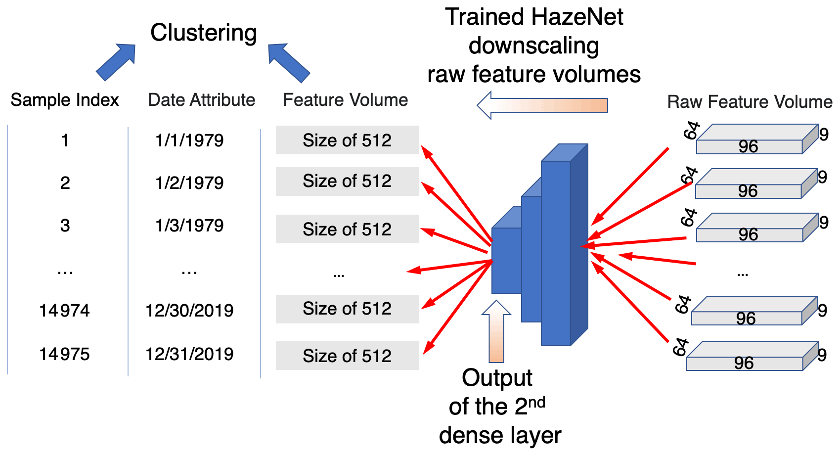
Figure 6A diagram of the cluster analysis procedure. Here 96, 64, and 9 represent the number of longitudinal grids, latitudinal grids, and features (variables) or the size of the input feature volume of a trained HazeNet for Beijing cases, respectively, while 512 is the size of the output from the dense layer before the output layer of HazeNet or the size of new feature volume.
In order to provide useful information for understanding the performance of the trained networks, the clustering has been performed for each of the prediction outcomes rather than just haze versus non-haze events (Appendix C). In this configuration, haze-associated regimes are represented by derived clusters of TP plus FN outcomes, while non-haze regimes are represented by clusters of TN plus FP outcomes. Since the clusters were derived using the indices of samples as the record for members, the actual feature maps of the members in any cluster can thus be conveniently retrieved and used to identify the representative regimes in terms of combined nine meteorological and hydrological features. Here the clustering results have been analyzed using the feature maps in both normalized (machine native) and unnormalized (original reanalysis data) format. The characteristics of various regimes can be easily identified from the former as they represent anomalies to climatological means. An added benefit is to advance the understanding of the performance of the trained networks. The analysis using the latter maps aims to better appreciate the conventional regional and local meteorological and hydrological patterns associated with various regimes. The feature maps used in both analyses have been averaged across each cluster for clarity.
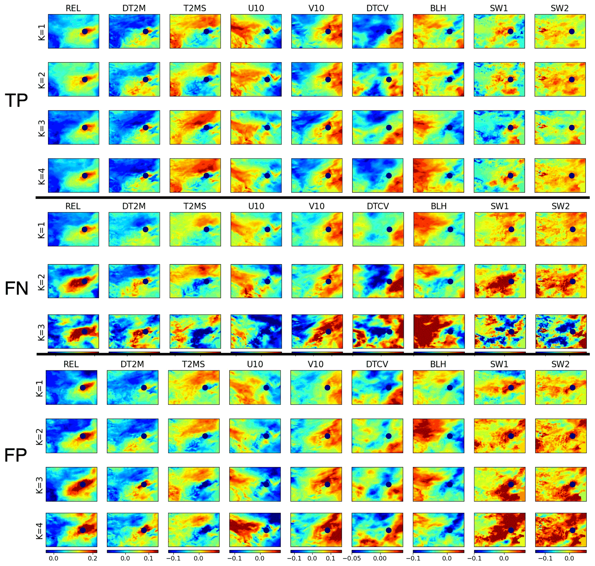
Figure 7Maps of the nine features in a normalized format for four clusters of true positive (TP) outcomes, three clusters of false negative (FN) outcomes, and four clusters of false positive (FP) outcomes. Here, TP plus FN covers haze events. Results shown are cluster averages for Beijing cases (location marked by navy dot).
4.1 Results based on normalized feature maps
As shown in Fig. 7, the four clusters of true positive (TP) cases in Beijing exhibit a clear similarity in general feature patterns closely surrounding Beijing (marked by a navy dot in the Fig. 7). These common patterns include an isolated small positive relative humidity (REL) center covering Beijing, associated with mild daytime change (DT2M) and standard deviation (T2MS) of surface temperature and zonal wind (U10) and a lower boundary layer height (BLH). Weatherwise, Beijing and its immediate surrounding area appear to be located between two sharply different air masses occupying the northwestern and southeastern part of the domain, respectively (weather systems usually progress from northwest to southeast in this region). When relating this to the other feature characteristics, it is likely that Beijing and its nearby area do not experience a drastic weather system change such as a front when haze occurs; hence, the high REL – a critical condition for aerosol to effectively scatter sunlight – can be easily formed, aided by a stable boundary layer with mild surface wind to allow aerosols to be well mixed vertically near the ground without being significantly reduced through advection diffusion. In addition, relatively high soil water content could fuel the humidity in the air, and thin while stable low clouds, if present (judged based on temperature change), could signal a lack of persistent precipitation. Altogether, these conditions apparently allow the haze to easily form, persist, and effectively scatter sunlight, thus reducing visibility. These conditions are also noticeably contrast with those associated with non-haze events represented by TN outcomes (Fig. S4).
Note that as each cluster consists of a collection of 3D data volumes or images, any two clusters could be sufficiently differentiated should only one of their images differ based on the clustering derivation algorithm, even though statistically speaking, they very likely belong to the same population (i.e., should be tested statistically). As shown in Fig. 7, the distinctions between TP clusters are largely reflected by the two different air masses distant from Beijing in both strength and spatial extent, particularly from DTCV patterns, likely representing different types of systems or background regimes. Specifically, a strong DTCV anomalous center seen in the cluster 1 and 4 patterns occupies most of the domain west of Beijing and directly influences Beijing and its nearby area. In contrast, DTCV distributions in cluster 2 and 3 are much weaker, where Beijing and its immediate neighboring area even appear to be more influenced by the southeastern system. In addition, surface wind distributions of the first two clusters clearly differ from those of cluster 3 and 4, and the patterns of BLH alongside SW1 and SW2 over Beijing and its immediate neighboring area of cluster 3 also suggest a land–atmosphere exchange condition differing from that of others. The combinations of these differences across various TP clusters apparently clearly define the various regimes of surrounding weather systems and their influence on Beijing. For the TP clusters of Shanghai, the above similarities and differences among various clusters also exist, except that clusters 1, 2, and 4 maintain more similarities in their feature patterns of distant air masses from Shanghai, while cluster 3 offers certain evident diversity in many feature patterns compared to other clusters (Fig. S5). Even more interestingly, the distribution of the number of members within various TP clusters evidently does not differ in different months (Table S1) (note that the number of haze events itself differs seasonally; see Fig. 5). Therefore, it is very likely that the characteristic weather conditions favoring haze occurrence and being captured by HazeNet cannot be simply differentiated by location (Beijing versus Shanghai) and season.
On the other hand, among three FN clusters (also associated with haze events but missed in prediction), only the first cluster (the major cluster of FN) displays certain similarity to TP clusters across various features. Even for this cluster, the characters of the air masses distantly surrounding Beijing differ substantially from those of TP clusters, as seen from the patterns of temperature (DT2M, T2SM), wind (particularly V10), and column water (DTCV) that reflect a much weaker weather system to the west. The patterns of BLH, SW1, and SW2 also differ from those of TP, indicating a different near-site boundary layer and hydrological condition. Such differences appear to be even more evident in the two other (minor) clusters, e.g., the size and strength of high relative humidity center covering Beijing are even more different. This result suggests a possible reason for HazeNet's inaccurate forecasting of these haze events, i.e., that haze might occur under unfavorable weather and hydrological conditions owing to, e.g., certain energy-consumption scenarios. Again, the distribution of members of these latter two clusters does not exhibit clear seasonality (Table S1). Interestingly, first two of the four FP clusters display more a clear similarity in their normalized feature patterns to those of TP than FN in Beijing and its immediate surrounding area (Fig. 7). As in FN cases, however, two other clusters differ more evidently. All of these could explain the false alarms reported by the machine, i.e., the machine could have simply been confused by such similarities between certain TP and FP members. Nevertheless, these could also suggest an alternative reason behind the incorrect forecasts, i.e., that certain pollution mitigation measures could have been in place. The results of FP clusters and the last FN cluster reported alongside a TP for Shanghai cases also share some similar characteristics as analyzed here (Figs. S5 and S6).
Therefore, it is worth indicating again that meteorological or hydrological conditions are not the only factors determining the occurrence of hazes. Other factors such as abnormal energy-consumption events or long-range transport of aerosols could all cause haze to occur even under unfavorable weather and hydrological conditions. This could well be the reason for some of the missing forecasts (FN outcomes) when haze occurred under unfavorable conditions, as suggested above, or for false alarms (FP outcomes) when low-aerosol events occurred even under a weather condition favorable to haze. Future improvement of the measurement skill could benefit from this knowledge.
4.2 Results based on original unnormalized feature maps
Utilizing feature maps in their original unnormalized format represented by actual physical quantities could provide a convenient way to appreciate the conventional regional and local meteorological and hydrological patterns and implement additional analysis, if necessary, of the possible impact of seasonality or trends associated with various events. Note that the visual differences between unnormalized feature maps, particularly in cluster mean format, might be too subtle for the naked eye to recognize.

Figure 8Feature maps associated with severe haze events in Beijing represented by four clusters of TP-predicted outcomes (four top rows) and three clusters of FN-predicted outcomes (three lower rows). Shown are cluster means of unnormalized data of relative humidity (REL) (ratio), daytime change (DT2M), and daily standard deviation (T2MS) of 2 m temperature (degrees), 10 m winds U10 and V10 (m/s), daytime change of column water vapor or DTCV (kg/m2), planetary boundary height (BLH) (m), and soil water content in soil level 1 (SW1) and level 2 (SW2) (kg/m2).
For haze events in Beijing (i.e., TP and FN outcomes; Fig. 8), the associated cluster mean regional meteorological and hydrological patterns of most features except DTCV contain two regions with sharply contrasting quantities, roughly separated by a line linking the southwest and northeast corner of the domain, likely due to the typical progression direction of weather systems in this region aside from a meridional variation of general climate. In comparison, the as same as is shown in the previous analysis using normalized feature maps, the patterns of the first FN cluster share many characteristics with those of TP clusters. The differences among TP and FN clusters are more evident in DTCV (specifically cluster 1 and 4 versus cluster 2 and 3), SW1, SW2, and surface winds, particularly for the second and third FN clusters. FP clusters also display a similarity to those of TP clusters (Fig. S7), whereas TN clusters show more visible differences, particularly in patterns of meridional wind (V10) and daily change of column water vapor or DTCV (Fig. S8).
The general regional meteorological and hydrological conditions during haze events in the southeastern portion, in contrast to the northwestern portion of the domain, include a higher relative humidity, lower variation of surface temperature, largely northward or northwestward wind, lower planetary boundary layer height, and higher soil water content, and quantity wise these are all in sharp contrast to the situation in the other half of the domain. Based on the surface wind direction, Beijing and its immediate surrounding area is clearly located between two air masses that both feature anticyclonic surface winds. The strengths of these two centers differ, particularly in the last two FN clusters, implying regimes with systems that have different strengths or that are in different development phases. Such a difference is also clearly related to the visually recognizable cross-cluster difference in DTCV patterns, represented by a strong negative center in the middle of the domain with varying extent and strength across different clusters. Consistent with the analysis result using normalized feature maps, all of these indicate a stable weather condition over Beijing and its neighboring area during haze events while surrounded by two (or more) different weather systems. It is known that dust can cause low-visibility events in Beijing. During dust seasons, the condition of the northwestern half of the domain, represented by a dominant eastward wind and lower soil water content, likely favors dust transport from desert to Beijing. However, the details would need an in-depth analysis since most clusters have members that are rather well distributed through different months (Table S1).
Table 1Cluster means of features associated with haze events (TP and FN) in Beijing and Shanghai versus means of all clusters of non-haze events of TN and FP. The number of cluster members in each cluster is listed in parentheses.
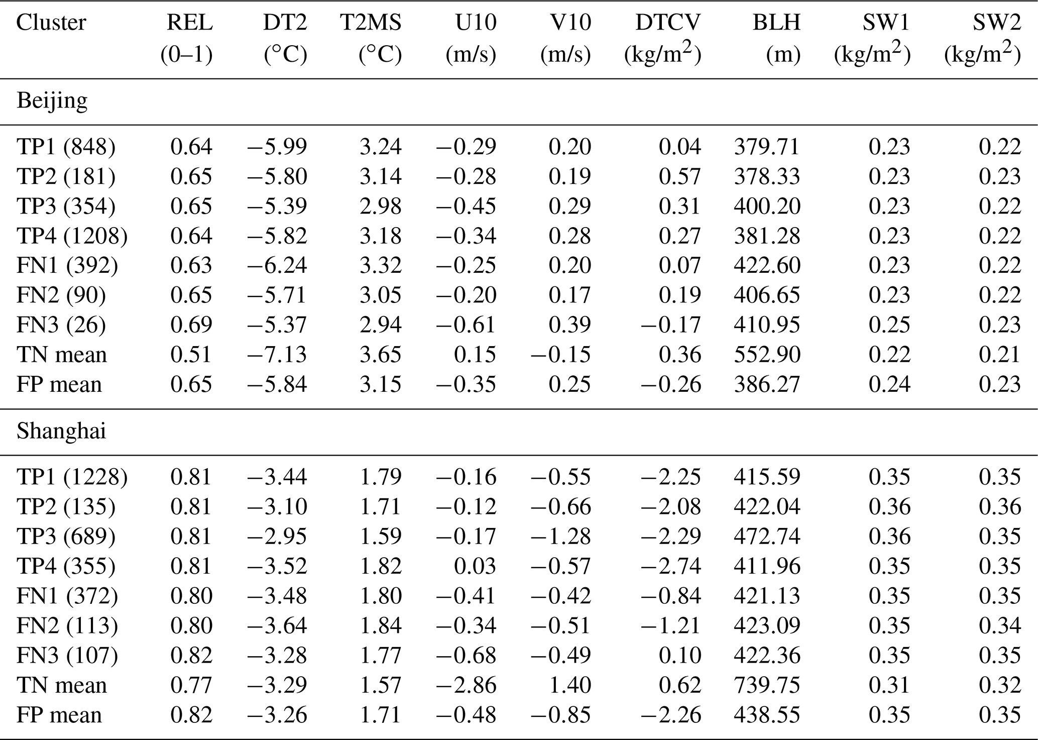
The cluster means of nine features for haze events (TP plus FN) versus non-haze (TN plus FP) at the grid point of Beijing are also derived and listed in Table 1 for reference. Specifically, the common local conditions associated with hazes in Beijing in comparison to those with non-haze events include a higher humidity, less drastic variations in surface temperature, a northwestward rather than southeastward wind, a lower planetary boundary layer height, and higher soil water content. Again, the most recognizable cross-cluster differences appear in DTCV (i.e., cluster 1 versus others), followed by surface wind (cluster 1 and 2 versus 3 and 4). In most of the local features, variabilities of FN clusters tend to be larger than those of TP clusters. Notably, such differences in local feature quantities for FN clusters are not necessarily more evident than in the regional maps over distant air masses. One interesting result of the local weather conditions shown in Table 1 is that the cluster means of TN are sharply different to those of TP and FN, while the cluster means of FP and those of TP + FN are likely to be statistically indifferent outside of DTCV, providing evidence to support the assumption that FP outcomes might simply represent the non-haze events caused by reasons other than weather and hydrological conditions.

Figure 9The same as Fig. 8 except for Shanghai with four clusters for TP outcomes and three clusters for FN outcomes.
For the case of Shanghai, the general weather conditions associated with haze events are likely stable, with characters similar to the cases of Beijing, except that Shanghai appears to be located between a northwest air mass with anticyclonic surface wind and a southeast air mass with cyclonic wind (Fig. 9). Quantities of most feature patterns display a sharply southeast versus northwest contrast. DTCV maps display a negative center over a large area, its distribution and extent vary significantly among different clusters in particular for the first two FN clusters. The patterns of soil water content in both soil layers exhibit a sharp meridional contrast that is much higher in the southern part of the domain than in the northern part, areas largely separated by the Yellow River. Local quantities of all the features associated with haze events (TP plus FN) in Shanghai display clear differences with those of non-haze prediction outcomes (TN) (Table 1). The most recognizable cross-cluster differences for TP appear in U10 of cluster 4 and V10 of cluster 3, differing from the cases of Beijing, and DTCV (particularly for cluster 3) for FN. Like the cases of Beijing, the cluster mean of the FP outcomes is not statistically different to that of haze (TP and FN) when compared to predicted non-haze (TN) events. Again, this result implies that even when a weather pattern favoring haze appeared and was correctly recognized by HazeNet, haze still could not to occur due to other factors such as energy-consumption variations.
It is worth indicating that the current analysis discussed here is only applied to the included features of clustering, and the presented figures in cluster-wise averaging format might have effectively smoothed out certain variability among members. A full-scale analysis would necessarily go beyond this to provide further synoptical or large-scale hydrological insights and better define different regimes.
Following an earlier preliminary attempt at forecasting haze in Singapore, a deep convolutional neural network containing more than 20 million parameters, HazeNet, has been further developed to test forecasting of the occurrence of severe haze events during 1979–2019 in two metropolitan areas in Asia, Beijing and Shanghai. By training the machine to recognize regional patterns of meteorological and hydrological features associated with haze events, the study advances our knowledge about this still poorly known environmental extreme. The deep CNN has been trained in a supervised learning procedure using time-sequential maps of up to 16 meteorological and hydrological variables or features as inputs and surface visibility observations as the labels.
Even with a rather limited sample size (14 975), the trained machine has displayed a reasonable performance measured by commonly adopted validation metrics. Its performance is clearly better during months with high haze frequency, i.e., all months except dusty April and May in Beijing and from late autumn through all of winter in Shanghai. Relatively large spatial patterns appear to be more effective than the smaller ones for influencing the performance of forecasting. On the other hand, in-depth analysis of performance results has also indicated certain limitations of the current approach of solely using meteorological and hydrological data in performing forecasts.
The trained machine has also been used to examine the sensitivity of the CNN to various input features and thus to identify and then remove features ineffective to the performance of the machine. In addition, to further categorize typical regional weather and hydrological patterns associated with severe haze versus non-haze events, an unsupervised cluster analysis has been subsequently conducted and has benefited from using features with greatly reduced dimensionality produced by using the trained machine.
The cluster analysis has, arguably for the first time, successfully categorized major regional meteorological and hydrological patterns associated with severe haze and non-haze events in Beijing and Shanghai into a limited number of representative groups, with the typical feature patterns of these clustered groups derived. It has been found that the typical weather and hydrological regimes of haze events in Beijing and Shanghai are rather stable conditions represented by anomalously high relative humidity, low planetary boundary layer height, and mild daily temperature change that are likely associated with a thin low cloud cover over the haze-occurring regions. The result has further revealed rather strong similarities in associated meteorological and hydrological regimes between haze and false alarm clusters and differences between haze and missing forecasting clusters, implying that factors such as energy-consumption variations, long-range transport of aerosols could influence the occurrence of hazes even under unfavorable weather conditions.
Due to the exploratory nature of this specific effort, several aspects could be further optimized, including the rather arbitrary though statistically meaningful labeling. In addition, an in-depth analysis of weather regimes would necessarily involve the use of certain features that are not included in the current clustering; however, this exceeds the extent of this paper and can only be discussed properly in a future work. Nevertheless, this study has demonstrated the potential of applying deep CNNs with extensive multi-dimensional and time-sequential environmental images to advance our understanding of poorly known environmental and weather extremes. Using this methodology, the results and experience obtained from this study could benefit future improvement efforts regarding these skills. Aside from this use, the trained machines can be used in many other types of machine learning and deep-learning applications, as has been partially demonstrated here.
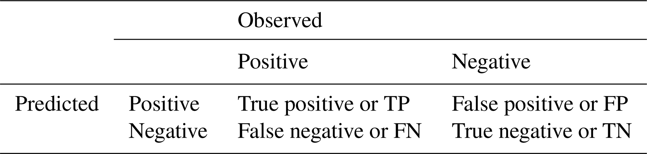
Several commonly used performance metrics have been used in this study. They are largely derived based on the so-called confusion matrix (Swets, 1988) as defined in the following Table A1.
Here, “positive” or “negative” is referring to the outcome of a given event or class in the classification, e.g., severe haze or non-haze events. Hence, the prediction outcome TP is a correct forecast of a severe haze, while TN is a correct forecast of a non-haze event, FP represents a false alarm, and FN represents a missing forecast. The context of outcomes changes when the designated class is switched. The major performance metrics used in this paper include
where
Here, F1 score is the F score with β=1 (van Rijsbergen, 1974), ETS represents equitable threat score (or Gilbert skill score; Gilbert, 1884; range ), HSS represents Heidke skill score (Heidke, 1926; range ), and N is the number of total outcomes. Note that “accuracy” has the same value for all the classes and thus is a good metric for the overall classification. The values of all the other metrics differ depending on the referred class.
Table A1Confusion matrix for measuring the prediction outcomes of a given class.
A method has been adopted in this study to use a trained machine to examine the sensitivity of the network to a random perturbation applied to the values of different features. The saved machine contains all the coefficients in different network layers and can be used to predict output from any of these layers using the same input features for training or validation. The sensitivity of the network to a given feature is determined by comparing the prediction using input feature maps containing random perturbation applied to the map of this feature with the prediction using original input feature maps. The sensitivity is measured by the content loss between these two predictions, with img1 with M×N pixels as the unperturbed and img2 as perturbed network output:
The perturbation is applied as random patches with the addition of −0.2 or 0.2 to 10 % of the pixels of the input map of the targeted feature in each sample, while maps of all the other features remain unperturbed. To reduce the workload, only the validation input set corresponding to the class 1 events (about 1020 samples) is used. Therefore, the sensitivity tested here is actually the sensitivity of the network to a given feature in predicting class 1 events. To preserve the spatial information of the perturbed field, the output of the 9th layer, or the “MaxPooling” layer following the second convolutional layer (Fig. 1), is used as the prediction. It has a size of (15, 31, 92) for Beijing cases and (15, 15, 92) for Shanghai cases when a kernel size of 20×20 is adopted. A higher content loss resulting from Eq. (B1) represents a higher sensitivity.
The cluster analysis of this study was conducted in the following three steps (see also Fig. 6).
- i.
Firstly, the trained and saved HazeNet for both the Beijing and Shanghai cases with nine input features have been used to perform prediction using the entire 14 975 input samples in the original raw data format, i.e., with a feature volume size of for Beijing and for Shanghai for each sample. The prediction results were then summarized into various outcomes, i.e., as true positive (TP), true negative (TN), false positive (FP), or false negative (FN), in referring to the haze class. In the meantime, the output of the second dense layer just before the output layer or the latent space (see Figs. 1 and 6) was further used to form a new data of each sample with a reduced feature volume of 512. This new dataset, with a size of 14 975 by 512, was then ready for clustering.
- ii.
The second step is to perform clustering using the new dataset with reduced size resulting from the previous step. For this purpose, it should be conducted separately for different types of samples or events, e.g., categorizing all the samples for haze into characteristic groups with similarities and identical features, and the same for all samples of non-haze events. In order to provide additional information to further the understanding of the network's performance, the clustering was actually conducted for different prediction outcomes, by taking corresponding samples from the new dataset. In this case, TP plus FN would lead to haze events, and TN plus FP would lead to non-haze events. The clustering calculations were done by directly using the k-mean (Steinhaus, 1957) function of the scikit-learn library (https://scikit-learn.org/stable/modules/clustering.html#clustering, last access: 2 September 2021). For Beijing cases, the trained machine with nine features produced 2591 TP, 11368 TN, 508 FP, and 508 FN outcomes, and it produced 2407 TP, 11 484 TN, 492 FP, and 592 FN outcomes for Shanghai. The cluster analysis was performed separately for each of these outcomes in an unsupervised learning procedure to let the machine categorize corresponding samples into groups based on similarities among them. In practice, similarity is judged by the so-called inertia for a cluster with members of xi and mean of μ:
The clustering is to seek a grouping with minimized inertia within each cluster. The overall measure is the summation inertia that decreases almost exponentially with the increase of number of clusters. In practice, the cluster analysis was first tested with various given number of clusters ranging from 1 to 100 to examine the values alongside decay of the inertia. This provided a base to identify the smallest possible number of cluster centers with reasonably low inertia in actual cluster analysis. This has actually been decided by using square root of the inertia weighted by the number of samples to put the varying number of samples across various outcomes in consideration. An optimized number of clusters was chosen with a weighted inertia lower than of that of the single-cluster case. For TN, due to the large sample number, this criterion was set to be half of . As a result, the optimized number of clusters for TP, FN, FP, and TN outcomes is 4, 3, 4, and 15 for Beijing and 4, 3 3, and 10 for Shanghai, respectively.
- iii.
The members of each cluster derived from step (ii) were recorded by the actual sample indices with the date included. Therefore, actual samples of input data grouped into various clusters can be conveniently identified with corresponding feature maps retrieved, either in a normalized or unnormalized format (i.e., in original quantity as in reanalysis dataset), and used for further analyses. In practice, cluster-averaged maps for various features were performed beforehand.
The Python script for network architecture, training, and validation is rather straightforward and simple, basically consisting of directly adopted function calls from Keras interface library (https://github.com/keras-team/keras, last access: 2 September 2021) with a TensorFlow-GPU (https://www.tensorflow.org, last access: 2 September 2021) as the backend or from scikit-learn library (https://scikit-learn.org/, last access: 2 September 2021). All the data used here for the analyses are publicly available: GSOD data from https://www.ncei.noaa.gov/access/metadata/landing-page/bin/iso?id=gov.noaa.ncdc:C00516, last access: 2 September 2021; ERA5 reanalysis data from https://climate.copernicus.eu/climate-reanalysis, last access: 2 September 2021.
The supplement related to this article is available online at: https://doi.org/10.5194/acp-21-13149-2021-supplement.
The author declares that there are no conflicts of interest.
Publisher's note: Copernicus Publications remains neutral with regard to jurisdictional claims in published maps and institutional affiliations.
This study is supported by L'Agence National de la Recherche (ANR) of France under “Programme d'Investissements d'Avenir” (ANR-18-MPGA-003 EUROACE). The author thanks the European Centre for Medium-range Weather Forecasts for making the ERA5 data publicly available under a license generated (and service offered) by the Copernicus Climate Change Service and the National Center for Environmental Information of the US NOAA for making the GSOD data available. All of the related computations have been accomplished using the GPU clusters of French Grand Equipment National de Calcul Intensif (GENCI) (project 101056) and the CNRS Mesocenter of Computing of CALMIP (project p18025). Constructive comments and suggestions from two anonymous reviewers led to the improvement of the manuscript.
This research has been supported by the Agence Nationale de la Recherche (grant no. ANR-18-MPGA-003 EUROACE).
This paper was edited by Yun Qian and reviewed by two anonymous referees.
Chan, C. K. and Yao, X.: Air pollution in mega cities in China, Atmos. Environ., 42, 1–42, 2008.
Chattopadhyay, A., Nabizadeh, E., and Hassanzadeh, P.: Analog forecasting of extreme-causing weather patterns using deep learning, J. Adv. Model. Earth Sy., 12, e2019MS001958, https://doi.org/10.1029/2019MS001958, 2020.
Forest, D.: Generative Deep Learning, O'Reilly Media, Inc., Sebastopol, CA, 2019.
Gagne, D., Haupt, S., and Nychka, D.: Interpretable deep learning for spatial analysis of severe hailstorms, Mon. Weather Rev., 147, 2827–2845, https://doi.org/10.1175/MWR-D-18-0316.1, 2019.
Gilbert, G. K.: Finley's tornado predictions, Amer. Meteor. J., 1, 166–172, 1884.
Goodfellow, I., Bengio, Y. and Courville, A.: Deep Learning, MIT Press, Cambridge, MA, 800 pp., 2017.
Grover, A. Kapoor, A., and Horvitz, E.: A deep hybrid model for weather forecasting, Proc. 21st ACM SIGKDD Intern'l Conf. KDD, 10 August 2015, Sydney, Australia, ACM, 379–386, https://doi.org/10.1145/2783258.2783275, 2016.
He, K., Zhang, X., Ren, S., and Sun, J.: Deep residual learning for image recognition, arXiv:1512.03385, 2015.
Heidke, P.: Calculation of the success and goodness of strong wind forecasts in the storm warning service, Geogr. Ann. Stockholm, 8, 301–349, 1926.
Hersbach, H., Bell, B., Berrisford, P., Hirahara, S., Horányi, A., Muñoz-Sabater, J., Nicolas, J., Peubey, C., Radu, R., Schepers, D., Simmons, A., Soci, C., Abdalla, S., Abellan, X., Balsamo, G., Bechtold, P., Biavati, G., Bidlot, J., Bonavita, M., De Chiara, G., Dahlgren, P., Dee, D., Diamantakis, M., Dragani, R., Flemming, J., Forbes, R., Fuentes, M., Geer, A., Haimberger, L., Healy, S., Hogan, R. J., Hólm, E., Janisková, M., Keeley, S., Laloyaux, P., Lopez, P., Lupu, C., Radnoti, G., de Rosnay, P., Rozum, I., Vamborg, F., Villaume, S., and Thépaut, J.-N.: The ERA5 global reanalysis, Q. J. Roy. Meteor. Soc., 146, 1999–2049, 2020.
Ioffe, S. and Szegedy, C.: Batch normalization: Accelerating deep network training by reducing internal covariate shift, arXiv:1502.03167, 2015.
Jiang, G.-Q., Xu, J., and Wei, J.: A deep learning algorithm of neural network for the parameterization o typhoon-ocean feedback in typhoon forecast models, Geophys. Res. Lett., 45, https://doi.org/10.1002/2018GL077004, 2018.
Kiehl, J. T. and Briegleb, B. P.: The relative roles of sulfate aerosols and greenhouse gases in climate forcing, Science, 260, 311–314, 1993.
Kurth, T., Treichler, S., Romero, J., Mudigonda, M., Luehr, N., Phillips, E., Mahesh, A., Matheson, M., Deslippe, J., Fatica, M., Prabhat, and Houston, M.: Exascale deep learning for climate analytics, arXiv:1810.01993, 2018.
Lagerquist, R., McGovern, A., and Gagne II, D.: Deep learning for spatially explicit prediction of synoptic-scale fronts, Weather Forecast., 34, 1137–1160, https://doi.org/10.1175/WAF-D-18-0183.1, 2019.
LeCun, Y., Bengio, Y., and Hinton, G.: Depp learning, Nature, 521, 436–444, https://doi.org/10.1038/nature14539, 2015.
Lee, H.-H., Bar-Or, R. Z., and Wang, C.: Biomass burning aerosols and the low-visibility events in Southeast Asia, Atmos. Chem. Phys., 17, 965–980, https://doi.org/10.5194/acp-17-965-2017, 2017.
Lee, H.-H., Iraqui, O., Gu, Y., Yim, S. H.-L., Chulakadabba, A., Tonks, A. Y.-M., Yang, Z., and Wang, C.: Impacts of air pollutants from fire and non-fire emissions on the regional air quality in Southeast Asia, Atmos. Chem. Phys., 18, 6141–6156, https://doi.org/10.5194/acp-18-6141-2018, 2018.
Lee, H.-H., Iraqui, O., and Wang, C.: The impacts of future fuel consumption on regional air quality in Southeast Asia, Sci. Rep.-UK, 9, 2648, https://doi.org/10.1038/s41598-019-39131-3, 2019.
Lin, Y., Wijedasa, L. S., and Chisholm, R. A.: Singapore's willingness to pay for mitigation of transboundary forest-fire haze from Indonesia, Environ. Res. Lett., 12, 024017, https://doi.org/10.1088/1748-9326/aa5cf6, 2016.
Liu, M., Huang, Y., Ma, Z., Jin, Z., Liu, X., Wang, H., Liu, Y., Wang, J., Jantunen, M., Bi, J., and Kinney, P. L.: Spatial and temporal trends in the mortality burden of air pollution in China: 2004–2012, Environ. Int., 98, 75–81, 2017.
Liu, Y., Racah, E., Prabhat, Correa, J., Khosrowshahi, A., Lavers, D., Kunkel, K., Wehner, M., and Collins, W.: Application of deep convolutional neural networks for detecting extreme weather in climate datasets, arXiv:1605.01156, 2016.
McGovern, A., Lagerquist, R., Gagne II, D. J., Jergensen, G. E., ElmLMore, K. L., Homeyer, C. R., and Smith, T.: Making the black box more transparent: Understanding the physical implications of machine learning, B. Am. Meteorol. Soc., 100, 2175–2199, 2019.
Ronneberger, O., Fischer, P., and Brox, T.: U-Net: Convolutional networks for biomedical image segmentation, arXiv:1505.04597, 2015.
Shi, X., Chen, Z., Wang, H., and Yeung, D.-Y.: Convolutional LSTM network: A machine learning approach for precipitation nowcasting, arXiv:1506.04214, 2015.
Silva, R. A., West, J. J., Zhang, Y., Anenberg, S. C., Lamarque, J.-F., Shindell, D. T., Collins, W. J., Dalsoren, S., Faluvegi, G., Folberth, G., Horowitz, L. W., Nagashima, T., Naik, V., Rumbold, S., Skeie, R., Sudo, K., Takemura, T., Bergmann, D., Cameron-Smith, P., Cionni, I., Doherty, R. M., Eyring, V., Josse, B., MacKenzie, I. A., Plummer, D., Righi, M., Stevenson, D. S., Strode, S., Szopa, S., and Zeng, G.: Global premature mortality due to anthropogenic outdoor air pollution and the contribution of past climate change, Environ. Res. Lett., 8, 034005, https://doi.org/10.1088/1748-9326/8/3/034005, 2013.
Simonyan, K. and Zisserman, A.: Very deep convolutional networks for large-scale image recognition, arXiv:1409.1556, 2015.
Smith, A., Lott, N., and Vose, R.: The integrated surface database: Recent developments and partnerships, B. Am. Meteorol. Soc., 92, 704–708, https://doi.org/10.1175/2011BAMS3015.1, 2011.
Steinhaus, H.: Sur la division des corps matériels en parties, Bull. Acad. Polon. Sci., 4, 801–804, 1957.
Swets, J.: Measuring the accuracy of diagnostic systems, Science, 240, 1285–1293, 1988.
Szegedy, C., Vanhoucke, V., Ioffe, S., Shlens, J., and Wojna, Z.: Rethinking the inception architecture for computer vision, arXiv:1512.00567, 2015.
van Rijsbergen, C.: Foundation of evaluation, J. Documentation, 30, 365–373, 1974.
Wang, C.: Exploiting deep learning in forecasting the occurrence of severe haze in Southeast Asia, arXiv:2003.05763, 2020.
Weyn, J. A., Durran, D. R., and Caruana, R.: Improving data-driven global weather prediction using deep convolutional neural networks on a cubed sphere, J. Adv. Model. Earth Sy., e2020MS002109, https://doi.org/10.1029/2020MS002109, 2020.
- Abstract
- Introduction
- Network architecture, training methodology, and data
- Training and validation results of haze forecasting
- Identifying and categorizing the typical regional meteorological and hydrological regimes associated with haze events
- Summary and conclusions
- Appendix A: Performance metrics
- Appendix B: Examining the network's sensitivity to features using trained machine
- Appendix C: Cluster analysis
- Code and data availability
- Competing interests
- Disclaimer
- Acknowledgements
- Financial support
- Review statement
- References
- Supplement