the Creative Commons Attribution 4.0 License.
the Creative Commons Attribution 4.0 License.
 | 18 Aug 2021
Fifty years of balloon-borne ozone profile measurements at Uccle, Belgium: a short history, the scientific relevance, and the achievements in understanding the vertical ozone distribution
Roeland Van Malderen
Dirk De Muer
Hugo De Backer
Deniz Poyraz
Willem W. Verstraeten
Veerle De Bock
Andy W. Delcloo
Alexander Mangold
Quentin Laffineur
Marc Allaart
Frans Fierens
Valérie Thouret
Starting in 1969 and comprising three launches a week, the Uccle (Brussels, Belgium) ozonesonde dataset is one of longest and densest in the world. Moreover, as the only major change was the switch from Brewer-Mast (BM) to electrochemical concentration cell (ECC) ozonesonde types in 1997 (when the emissions of ozone-depleting substances peaked), the Uccle time series is very homogenous. In this paper, we briefly describe the efforts that were undertaken during the first 3 decades of the 50 years of ozonesonde observations to guarantee the homogeneity between ascent and descent profiles, under changing environmental conditions (e.g. SO2), and between the different ozonesonde types. This paper focuses on the 50-year-long Uccle ozonesonde dataset and aims to demonstrate its past, present, and future relevance to ozone research in two application areas: (i) the assessment of the temporal evolution of ozone from the surface to the (middle) stratosphere, and (ii) as the backbone for validation and stability analysis of both stratospheric and tropospheric satellite ozone retrievals. Using the Long-term Ozone Trends and Uncertainties in the Stratosphere (LOTUS) multiple linear regression model (SPARC/IO3C/GAW, 2019), we found that the stratospheric ozone concentrations at Uccle have declined at a significant rate of around 2 % per decade since 1969, which is also rather consistent over the different stratospheric levels. This overall decrease can mainly be assigned to the 1969–1996 period with a rather consistent rate of decrease of around −4 % per decade. Since 2000, a recovery of between +1 % per decade and +3 % per decade of the stratospheric ozone levels above Uccle has been observed, although it is not significant and is not seen for the upper stratospheric levels measured by ozonesondes. Throughout the entire free troposphere, a very consistent increase in the ozone concentrations of 2 % per decade to 3 % per decade has been measured since both 1969 and 1995, with the trend since 1995 being in almost perfect agreement with the trends derived from the In-service Aircraft for a Global Observing System (IAGOS) ascent/descent profiles at Frankfurt. As the number of tropopause folding events in the Uccle time series has increased significantly over time, increased stratosphere-to-troposphere transport of recovering stratospheric ozone might partly explain these increasing tropospheric ozone concentrations, despite the levelling-off of (tropospheric) ozone precursor emissions and notwithstanding the continued increase in mean surface ozone concentrations. Furthermore, we illustrate the crucial role of ozonesonde measurements for the validation of satellite ozone profile retrievals. With the operational validation of the Global Ozone Monitoring Experiment-2 (GOME-2), we show how the Uccle dataset can be used to evaluate the performance of a degradation correction for the MetOp-A/GOME-2 UV (ultraviolet) sensors. In another example, we illustrate that the Microwave Limb Sounder (MLS) overpass ozone profiles in the stratosphere agree within ±5 % with the Uccle ozone profiles between 10 and 70 hPa. Another instrument on the same Aura satellite platform, the Tropospheric Emission Spectrometer (TES), is generally positively biased with respect to the Uccle ozonesondes in the troposphere by up to ∼ 10 ppbv, corresponding to relative differences of up to ∼ 15 %. Using the Uccle ozonesonde time series as a reference, we also demonstrate that the temporal stability of those last two satellite retrievals is excellent.
- Article
(4934 KB) - Full-text XML
-
Supplement
(1378 KB) - BibTeX
- EndNote


Ozone (O3) is a key trace gas in the Earth's atmosphere, where it mainly resides between the surface and the top of the stratosphere (about 50 km), with the highest concentrations in the lower to middle stratosphere (90 % of total column ozone amount). Ozone is mainly produced in the tropical stratosphere and transported to the lower stratosphere at high latitudes. Depending on its altitude, ozone is involved in different chemical reactions and, therefore, has a different impact on life on Earth. Stratospheric ozone absorbs the harmful solar ultraviolet (UV) radiation, thereby protecting life on Earth and warming the stratosphere. This protective shield has been in danger due to anthropogenic emissions of ozone-depleting substances (ODSs – such as chlorofluorocarbons, CFCs) since the 1970s, with the Antarctic springtime ozone hole as the most striking signature. Thanks to the Montreal Protocol (1987, and subsequent amendments and adjustments), positive trends in the ozone concentrations in the upper stratosphere have been observed since 2000 (WMO, 2018, chaps. 3 and 4; SPARC/IO3C/GAW, 2019). Ozone is also an important absorber of infrared (terrestrial) radiation, mainly in the tropopause region and can, therefore, act as a greenhouse gas at certain altitudes: it is estimated to have contributed ∼ 20 % as much positive radiative forcing as CO2 since 1750 (IPCC, 2013). Tropospheric ozone is also the main source of the OH free radical, the primary oxidant in the atmosphere, which is responsible for removing many compounds (including atmospheric pollutants) from tropospheric air. At the surface, ozone is an air pollutant that adversely affects human health, natural vegetation, and crop yield and quality (e.g. Cooper et al., 2014).
Because of the many roles of ozone, the knowledge and measurement of the vertical distribution of the ozone concentration in the atmosphere – and its variability in time – is crucial. Vertical ozone profiles can be obtained from ground-based instruments (Dobson/Brewer Umkehr, lidar, Fourier transform infrared spectrometer, and microwave radiometer), balloon-borne techniques (ozonesondes), and satellite-based measurements (using solar/stellar occultation, limb emission/scattering, and nadir-viewing techniques) (see e.g. Hassler et al., 2014, for details). In this research, we focus on ozonesondes, which are lightweight and compact balloon-borne instruments measuring the ozone concentration from the surface through the mid-stratosphere (about 10 hPa or 30 km). In electrochemical ozonesondes, atmospheric ozone is measured via an electrochemical reaction of ambient air bubbling in a solution of potassium iodide (KI), by means of a stable miniature pump. In a Brewer-Mast (BM) sonde, two electrodes of different metal are immersed in a buffered KI solution (Brewer and Milford, 1960), whereas electrochemical concentration cell (ECC) sondes consists of two half-cells with different solutions of KI as electrodes (Komhyr, 1969). The ozonesonde is launched in tandem with a radiosonde that also transmits air pressure, temperature, humidity, and wind data to a ground station. With a 20–30 s response time of the ozone cells and an ascent rate of about 6 m s−1, the effective vertical resolution of the ozone signal currently lies around 150 m. Before the digital sounding systems era, the vertical resolution was coarser due to the manual sampling technique by the operator, only providing measurements at significant levels.
Regular measurements with ozonesondes started in the second half of the 1960s at a few sites: in 1965 at Aspendale (Australia, but moved to other suburbs of Melbourne thereafter, i.e. Laverton and Broadmeadows), in 1966 at Resolute Bay (Canada), in 1967 at Hohenpeissenberg (Germany), in 1968 at Payerne (Switzerland) and at Tateno (Tsukuba, Japan), in 1969 at Uccle (Belgium) and Sapporo (Japan), and in 1970 at Wallops Island (USA). These ozone sounding stations provide the longest time series of vertical ozone distribution. Up to an altitude of about 30 km, ozonesondes constitute the most important data source with long-term data coverage for the derivation of ozone trends with sufficient vertical resolution, particularly in the climate-sensitive altitudinal region around the tropopause. Furthermore, ozonesondes are widely used to study photochemical and dynamical processes in the atmosphere or to validate and evaluate satellite observations and their long-term stability (Smit and ASOPOS panel, 2014, and references therein).
In this paper, we focus on the ozonesonde measurements at Uccle, covering 50 years, demonstrating the time series' scientific relevance and the major achievements. Ozonesondes are still the only technique able to measure the ozone concentration from the surface all the way up to the middle stratosphere with very high (absolute) accuracy and vertical resolution. Therefore, there are many application areas in which they are crucial, such as (i) quantifying the long-term variability in stratospheric and tropospheric ozone; (ii) as the backbone for satellite validation, with satellites mostly measuring ozone only in stratosphere or upper troposphere; and (iii) for process studies in stratospheric–tropospheric exchange and chemical production/destruction of ozone. The strength and uniqueness of the ozonesonde measurements, in particular of the long-term and very dense Uccle dataset, lie in combining all of these different aspects of ozone research. In this paper, we will first give a description of the ozonesonde measurements at Uccle from a historical point of view (Sect. 2) and briefly describe the data processing that has been applied to the ozonesonde measurements used in this paper (Sect. 3). In Sect. 4, we assess the time evolution of ozone at Uccle at different vertical layers against the background of recent findings in ozone variability. Section 5 illustrates the important role of the Uccle data for the validation of satellite ozone retrievals. Finally, in Sect. 6, concluding remarks and perspectives are given.
In this section, we give a brief overview of the history of the ozone measurements at Uccle (Brussels, Belgium: 50∘48′ N, 4∘21′ E; 100 m a.s.l.). We explain why the ozone-sounding programme was initiated more than 50 years ago and discuss the presence of a period of gaps in the time series (Sect. 2.1). We also describe which efforts have been undertaken during this time period to guarantee the homogeneity of the time series of ozonesondes between ascent and descent profiles (Sect. 2.2.1), with changing environmental conditions (Sect. 2.2.2), and between different ozonesonde types (Sect. 2.2.3). We only give a brief description here and refer the reader to the relevant earlier publications for more details.
2.1 The start of the ozone observations
The ozone-sounding programme at the Royal Meteorological Institute of Belgium (RMI) at Uccle was initiated by Jacques Van Mieghem, director of RMI from 1962 to 1970. Initially, the ozone soundings were not performed out of concern for possible anthropogenic influence on the ozone layer but rather to use ozone as a tracer to study the general air circulation in the troposphere and the lower stratosphere. Therefore, from the beginning, it was planned to perform regular ozone soundings three times per week (on Monday, Wednesday, and Friday).
In 1965 and 1966, the first few soundings were performed with Regener chemiluminescent ozonesondes, and these data are still available at the World Ozone and Ultraviolet Radiation Data Centre (WOUDC). A well-known effect of this sonde type is that it shows changes in sensitivity during the ascent trajectory (see e.g. Hering and Dütsch, 1965). For that reason, it was decided to switch to Brewer-Mast electrochemical ozonesondes (developed by Brewer and Milford, 1960, and commercially produced by the Mast Development Company at Iowa, USA) at RMI from November 1966 onwards. Based on a number of criteria, such as continuity of the measurements and how well the preparation of the sondes was documented, it was decided to use the ozone soundings for scientific studies only from 1969 onwards, when Dirk De Muer took over the ozone research at RMI (in July 1969).
In the period from February 1983 to January 1985, there were only a few ozone soundings. This gap in our time series was due to funding reductions. Later on, when the Uccle time series of ozone soundings had proved its scientific value and with the growing concern regarding the anthropogenic influence on the ozone layer, the continuation of the soundings became less an issue. In the course of time, different radio sounding systems have been used. A major change occurred in 1990 when digital data transmission at a high sampling rate was introduced, which allowed a higher vertical resolution of the profiles (not only at significant and standard pressure levels).
To normalize the integrated ozone amount of the ozone soundings (essential for BM ozonesondes; see Sect. 2.2.3), the Dobson spectrophotometer (no. 40, D40) at Uccle has been used since July 1971; before that date, an interpolation of values from other Dobson stations in the European network was employed. In 1984, the Uccle site was equipped with a single-Brewer UV spectrophotometer (no. 16), and in September 2001, it was equipped with a double-Brewer instrument (no. 178), to provide total ozone column measurements.
2.2 Challenges
2.2.1 Frequency response of the electrochemical ozonesonde
In 1970, the ozone-sounding programme was adapted to also gather data during the descent of the sonde after balloon burst. De Muer (1981) found that the measured ozone concentrations in the lower stratosphere and the troposphere were systematically higher during descent than during ascent (see Fig. 1, left panel). Two possible explanations were mentioned: (i) contamination of the ozonesonde during ascent (e.g. by reducing constituents in the atmospheric boundary layer; see Sect. 2.2.2) and/or (ii) the response time of the sensor. To investigate the latter, De Muer and Malcorps (1984) analysed the frequency response of the combined ozone sensor and air sampling system of Brewer-Mast ozonesondes by means of a Fourier analysis. They found three different time constants: (i) a first-order process with a time constant of about 17 to 25 s (depending on the solution temperature) caused by the formation of iodine in the solution; (ii) a time constant of 7 s, likely to be caused by the diffusion of iodine molecules to the platinum cathode; and (iii) a time constant of about 2.8 min that was explained by another diffusion process (i.e. an adsorption and subsequent desorption process of ozone at the surface of the air sampling system). The slow first-order process with a time constant of about 20–25 min (found by Salzman and Gilbert, 1959, and taken up by Vömel et al., 2020, and Tarasick et al., 2021) could not be identified, probably because the impact of this process for a 0.1 % KI solution would be too small (being 10 % of the fast process for a 1 % KI solution), as noted in De Muer and Malcorps (1984). With these findings and time constants, a method for deconvolution of the ozone profiles through a process of fast Fourier transform was developed, and an example of an ozone profile before and after deconvolution is also shown in Fig. 1 (right panel). After deconvolution, the observed ozone values during descent are still larger than the ascent values in the troposphere and the lowest layers in the stratosphere, which was then attributed to the effect of SO2 on the ozonesonde measurements in the boundary layer.
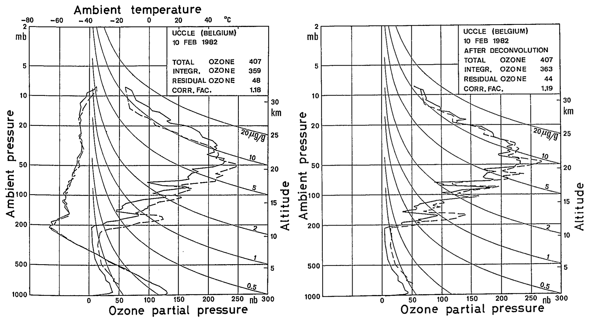
Figure 1Ozone sounding at Uccle on 10 February 1982 with a Brewer-Mast ozonesonde before (left) and after (right) deconvolution of the ozone profile for both ascent (solid line) and descent (dashed line) of the sonde. In the left panel, the vertical profile of the air temperature is also shown (figure taken from De Muer and Malcorps, 1984).
2.2.2 The impact of the boundary layer SO2 concentrations on the ozone measurements
Ozonesonde measurements by the KI method are sensitive to interference by oxidizing or reducing agents (e.g. Tarasick et al., 2021, and references therein). In particular, one SO2 molecule cause a reverse current of two electrons, reducing the electrochemical cell response on a 1 : 1 basis, and excess SO2 can accumulate in the cathode solution, affecting ozonesonde measurements well above the polluted boundary layer (Fig. 1 and Fig. S1 in the Supplement; Komhyr, 1969; De Muer and De Backer, 1993) or near volcanic sites (Morris et al., 2010). Furthermore, in the case of a considerable total vertical SO2 column amount, the Dobson total ozone amounts might be overestimated, as SO2 has even stronger absorption bands than ozone in the UV 305–340 nm wavelength range used for the total ozone determination (Komhyr and Evans, 1980). As a matter of fact, in the suburban area of Uccle, the SO2 densities near the ground were quite elevated at the start of the ozone measurements but showed a steep decrease from the late 1960s to the early 1990s (Fig. S2).
As a consequence, the variation in SO2 density near the ground has a twofold effect on ozone soundings with electrochemical sondes: (i) the integrated ozone amount of the (BM) soundings is normalized by means of spectrophotometer data, so that a trend in the latter data will lead to an effect on ozone trends from soundings; and (ii) due to the SO2 interference with the ozonesonde cell reactions, any trend in SO2 causes a distortion of ozone profile trends as a function of altitude.
To minimize this twofold impact of SO2 on the ozonesonde ozone measurements, two corrections were developed. Based on the comparison between quasi-simultaneous total ozone observations at Uccle with a Dobson and a Brewer spectrophotometer (De Backer and De Muer, 1991), a model connecting SO2 column readings with long-term surface SO2 monitoring measurements was able to subtract a fictitious trend in the Dobson. Applying this correction made the Dobson total ozone trend consistent with both the Brewer trend and the one derived from reprocessed Total Ozone Mapping Spectrometer (TOMS) satellite data for the sub-periods in which both datasets were available (De Muer and De Backer, 1992). Furthermore, a method to calculate the vertical SO2 distribution associated with each ozone sounding was developed based on two assumptions: (i) a constant SO2 mixing ratio from the ground to the mixing layer height and (ii) an exponentially decreasing mixing ratio above the mixing layer balancing the integrated SO2 amount to the reduced thickness of the SO2 layer (De Muer and De Backer, 1993). The effect of those two corrections for SO2 interference on the vertical ozone trends in the 1969–1996 Brewer-Mast period is illustrated in Fig. S3. It shows that these corrections are essential in assessing the trends in tropospheric ozone at Uccle until the mid-1990s.
2.2.3 The transition from BM to ECC sondes
As mentioned before, at the start of the operational ozone-sounding series, the Brewer-Mast sensor type was used. This type of ozonesonde had several issues at that time: (i) a strong reduction of the efficiency of the pump at low pressure (De Backer et al., 1998a); (ii) the loss of ozone in the sensor itself, causing a relatively high (up to 20 %) underestimation of the integrated ozone from a sounding profile with respect to the total ozone measured with a Dobson or a Brewer spectrophotometer; and (iii) a variable response in the troposphere, depending on preparation (Tarasick et al., 2002).
Therefore, in the middle of the 1990s, RMI investigated the switch from the BM sondes to the ECC (En-Sci) sensors (Komhyr, 1969), which seemed to perform better and were easier to prepare before launch. To document this transition, dual soundings were launched about twice a month during 1 year. The comparison between both sensor types on those dual soundings is shown in Fig. S4. If standard correction methods for both sensors are used, large statistically significant differences appear: Brewer-Mast sensors overestimate tropospheric ozone and underestimate stratospheric ozone, mainly due to the standard normalization by linear scaling of the vertical ozone profile for BM sondes. Therefore, De Backer et al. (1998a, b) developed one “PRESsure- and Temperature-dependent Total Ozone normalization” (now called PRESTO; see Van Malderen et al., 2016) correction method for both ozonesonde types based on (i) measurements of the pump efficiencies of both ozonesonde types in a pressure chamber at Uccle, (ii) a preflight comparison of every ozonesonde with a calibrated ozone source in the lab, and (iii) the comparison with the total ozone column measured with the co-located ozone spectrophotometer (full practical details are available in De Backer, 1999). This method is still the operational approach at Uccle and has been used to process all of the ozonesonde data used in this work (see Sect. 3). By applying this method, the differences between the dual ozone-sounding profiles are reduced below 3 % throughout almost the whole profile and below the statistical significance level (Fig. S4). The impact of this new pump correction method on the vertical ozone trends is also significant, especially for the 1969–1996 BM period (see Fig. S3; for other periods, see Van Malderen et al., 2016).
Further validation of the method was undertaken by comparing the profiles with measurements from the SAGE II satellite instrument (Lemoine and De Backer, 2001). This study showed that the PRESTO correction removed the jump, caused by the BM to ECC transition, in the difference time series with SAGE II at low pressures (cf. Figs. 1 and 2 in Lemoine and De Backer, 2001).
In this paper, the PRESTO correction has been applied to the entire ozonesonde dataset (i.e. to both the BM and ECC (En-Sci) ozonesonde types) with the appropriate different measured pump efficiency coefficients at Uccle for both ozonesonde types in order to ensure consistency over the entire data record of 50 years. Although a total ozone normalization is not required for the ECC sonde measurements (Smit and ASOPOS panel, 2014), it is applied for the entire Uccle time series within the PRESTO correction. To calculate the residual ozone above the balloon burst level, we use a combination of the constant mixing ratio approach and the climatological mean obtained from satellite ozone retrievals (McPeters and Labow, 2012). An alternative, homogenized, corrected ozonesonde dataset for Uccle is available upon request from the authors for the ECC time series since 1997 (Van Malderen et al., 2016), following the principles of the Ozonesonde Data Quality Assessment (O3S-DQA) activity (Smit et al., 2012), but it is not used here to maintain consistency over the entire time series. Differences between both versions of corrected Uccle ECC ozonesonde data, in comparison with the nearby De Bilt (the Netherlands, 175 km north of Uccle) ozonesonde site, are highlighted in Van Malderen et al. (2016).
For the BM ozonesondes, the applied PRESTO corrections include (i) a correction for SO2 interference on the ozone soundings (imperative for reliable lower tropospheric ozone trend estimates for the 1969–1996 period; see Fig. S3), (ii) a correction for a negative background current caused by impurities in the sensor before October 1981, (iii) a correction for box temperatures depending on the insulating capacity of the Styrofoam boxes (a short discussion of those additional corrections and the proper references are given in the Appendix A of Van Malderen et al., 2016), and (iv) an altitude correction for VIZ/Sippican radiosonde pressure measurements based on comparisons with wind-finding radar. Without this altitude correction, sonde altitudes were too low up to 1000 m at an altitude of 30km, so that the calculated ozone concentrations with VIZ radiosondes were too low by 7.5 % to 14 %, depending on the manufacturing series of radiosondes (De Muer and De Backer, 1994). Since 1990, the ozonesondes at Uccle have been combined with Vaisala RS80 radiosondes, which showed a much smaller difference in the calculated altitude with respect to wind-finding radar data. Therefore, for the digital era period since 1990, no radiosonde pressure sensor bias corrections have been applied, although biases have been identified in different studies (e.g. De Backer, 1999; Steinbrecht et al., 2008; Stauffer et al., 2014; Inai et al., 2015).
As ozonesondes are the only devices that are able to measure ozone concentrations from the surface up to the middle stratosphere with high vertical resolution, they are very suitable to study and relate the temporal variability of ozone in different atmospheric layers. The evaluation of the temporal variability of the ozone measurements at Uccle is, therefore, organized into different sections. We first describe the stratospheric (Sect. 4.1) and tropospheric (Sect. 4.2) ozone trends. The relation to other co-located ozone measurements is described in the appendices. Total ozone trends are treated in Appendix A, and the temporal behaviour of surface ozone and several ozone-depleting substances is discussed in Appendix B.
4.1 Stratospheric ozone trends
To calculate the vertical distribution of trends in the stratospheric ozone concentrations from the Uccle ozonesonde data, we use the altitude relative to the tropopause height as the vertical coordinate. The tropopause applied here is the standard (first) thermal tropopause (WMO, 1957) and is derived from the vertical temperature profiles measured by the Uccle radiosondes, as described in Van Malderen and De Backer (2010). The implemented statistical model to calculate trends is the Long-term Ozone Trends and Uncertainties in the Stratosphere (LOTUS) multiple linear regression (MLR) model (SPARC/IO3C/GAW, 2019). This model uses an independent linear trend (ILT) method as trend term, which is based on two different, independent, trends to describe the ozone decrease until 1997 (ODS increase) and the slow ozone increase since the early 2000s (after the turnaround in ODS concentrations). These two periods have been used since WMO (2014), and their use avoids end-point anomalies near the turnaround in 1997 for the two independent linear trend terms in the ILT method. Additionally, the LOTUS regression includes two orthogonal components of the Quasi-biennial Oscillation (QBO), the 10.7 cm solar radio flux, the El Niño–Southern Oscillation (ENSO) without any lag applied, and the aerosol optical depth (AOD, extended past 2012 by repeating the final available value from 2012 as the background AOD, which should be a valid assumption for Uccle). Four Fourier components representing the seasonal cycle are also included, unless (relative) monthly anomaly series are used as input ozone data. The output of the LOTUS MLR model and the different contributing terms (or proxies) for the monthly anomaly ozone concentrations at the layer 10 km above the tropopause (close to the ozone peak) are shown in Fig. S5. The final choice of those proxies (and possible lags) in LOTUS was based on retaining the optimal regression for the global analysis of satellite data and broad latitude band analyses. Therefore, proxies describing rather local or small-scale phenomena might not have been included in the general “LOTUS regression” model. In particular, using an alternative stepwise multiple linear regression model for the Uccle stratospheric ozone amounts, we found that the Uccle tropopause pressure and the Arctic Oscillation are significant proxies as well (contributing statistically significant, i.e. at the 95 % significance level of the t test, to the regression coefficient). However, here, the analysis is limited to the LOTUS model, and the sensitivity of the estimated trends on the chosen (M)LR model is rather limited for the Uccle time series.
The vertical profile of stratospheric ozone trends is shown in Fig. 2. From 1969 to 1997, stratospheric ozone concentrations decrease almost uniformly (and significantly) at a rate of around −4 % per decade, except at the layers just above the tropopause. Since 2000, the stratospheric ozone concentrations have increased by about +2 % per decade but only significantly at the layers below and at the ozone maximum (from 6 to 13 km above the tropopause, or 17 to 24 km for an average tropopause height of 11 km at Uccle). The insignificant negative trend in the Uccle ozone concentrations at the upper levels of Fig. 2 should be treated with caution, as the reliability of the ozonesonde instrument at those levels (above 30 km) is reduced. This is due to the increasing uncertainty in the pump efficiency at low pressures, the different stoichiometry of the chemical reaction due to a reduced amount of sensing solutions by evaporation, and frozen solutions. Additionally, an increase in the burst altitude in the Uccle ozonesonde time series in recent years and inhomogeneities due to changing pressure sensors with different radiosonde types might have had an impact on the ozone trends at these very low pressures. In fact, the negative ozone trends are also less pronounced if calculated for absolute altitude levels. However, for these altitudes, we also prefer to calculate the vertical ozone trends in altitudes relative to the tropopause in order to cancel out the seasonal variation of the ozone peak altitude, which roughly follows the tropopause height variation at Uccle: the ozone maximum peak is at its highest altitudes in summer (when the tropopause is also located higher) and is located at lower altitudes in winter (with the lowest tropopause). This approach generally gives vertical ozone trends that vary less over the different altitude levels. When we compare the post-2000 trends with those from the ozonesondes launched at De Bilt, the overall stratospheric positive insignificant trends apply for both stations, also at the higher altitude levels at De Bilt. The larger trend uncertainties for the De Bilt time series can be explained by the lower frequency of launches (once a week versus three times a week at Uccle). The statistically insignificant offset between the Uccle and De Bilt trend estimates depends on the correction methods used at both sites, but differences in the vertical ozone distribution (up to 5 % in the stratosphere), of both geophysical and instrumental origin, also have an impact on the trend values (see e.g. Figs. 10a and 12 in Van Malderen et al., 2016, in which a more detailed explanation of the differences in vertical ozone distribution and trends between Uccle and De Bilt is given).
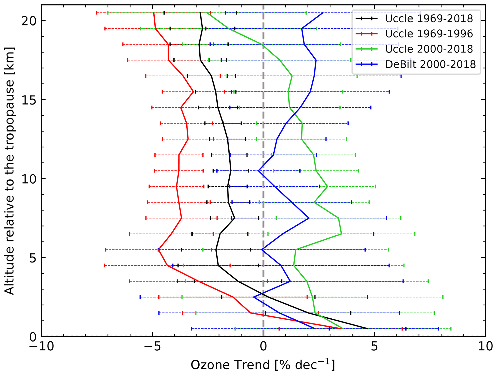
Figure 2Vertical distribution of trends in stratospheric ozone concentrations at Uccle for different periods (see text) and at De Bilt (2000–2018). The trends and their uncertainties are calculated with the LOTUS multiple linear regression model (see text and SPARC/IO3C/GAW, 2019), including an independent linear trend term. The 2σ error bars represent the trend uncertainty estimated by the regression model (using the fit residuals). For the Uccle 1969–2018 time series only, one linear trend term is included in the model instead. The output of the LOTUS MLR model and the different contributing terms for the monthly anomaly ozone concentrations at the layer 10 km above the tropopause are shown in Fig. S5.
The lower stratospheric ozone trends deserve more discussion here, as Ball et al. (2018, 2019) reported a significant decline in lower stratospheric (13–24 km) ozone amounts for the respective 1998–2016 and 1998–2018 periods from multiple (merged) satellite measurements in the lower stratosphere between 60∘ N and 60∘ S. Moreover, the latest Scientific Assessment of Ozone Depletion (WMO, 2018), largely based on the LOTUS final report (SPARC/IO3C/GAW, 2019), concluded that “there is some evidence for a decrease in lower stratospheric ozone from 2000 to 2016”, although not statistically significant in most analyses. This decline, contradictory to the decline in ozone-depleting substances since 1997, is surprising, and the current state-of-the-art chemistry climate models (CCMs) used in Ball et al. (2020) and Dietmüller et al. (2021) do not show a decrease but rather an increase in the lower stratospheric mid-latitude ozone, although they confirm the lower stratospheric ozone decline in the tropics in the observations. Using the Modern-Era Retrospective Analysis for Research and Applications Version 2 (MERRA-2) ozone output fields, Wargan et al. (2018) found a discernible negative trend of −1.67 ± 0.54 Dobson units per decade in the 10 km layer above the tropopause between 20 and 60∘ N, and they attributed the trend to changes driven by dynamical variations (as in Chipperfield et al., 2018), in the form of enhanced isentropic mixing between the tropical (20∘ S–20∘ N) and extratropical lower stratosphere over the past 2 decades. In a follow-up study, Orbe et al. (2020) demonstrated that in the Northern Hemisphere (NH), this mid-latitude ozone decrease is primarily associated with changes in the advective circulation rather than changes in mixing. In this study, both the Uccle and De Bilt time series do not show a significant decline in lower stratospheric (13–24 km) ozone amounts. On the contrary, although never significant, we found that the positive Uccle ozone trends in the lower stratosphere are rather robust, independent of the starting date (1997/1998/2000), the vertical coordinate system used (absolute or relative to the tropopause), and the trend model used (LOTUS MLR or simple linear fit). The lower stratospheric ozone trends derived from the De Bilt time series show a larger variability between positive and negative statistically insignificant values, especially in the lowest 10 km.
Ball et al. (2020) investigated if the aforementioned changes in ozone and transport are also found in other stratospheric variables like the temperature. Globally, a reduction in lower stratospheric ozone should lead to reduced radiative heating and a decrease in observed temperature (see references in Ball et al., 2020). Quasi-global lower stratospheric temperatures from observations and in CCMs indeed decreased, with the post-2000 negative temperature trend being smaller compared with pre-1998, mimicking the observed lower stratospheric ozone trends (Ball et al., 2020; but also Maycock et al., 2018), although not the modelled ozone increase after 2000. On a smaller (European) scale, Philipona et al. (2018) found very similar seasonal and annual changes for temperature and ozone when averaging the Payerne, Hohenpeissenberg, and Uccle ozonesonde measurements. With the exception of the fall season, annual and seasonal profiles switch from negative to positive trends before and after the turn of the century for both ozone and temperature (see Fig. 4 in Philipona et al., 2018). Here, on the local scale of Uccle and De Bilt, we also investigated the link between the lower stratospheric ozone and temperature trends (see Fig. S6). Before 1997, the entire stratosphere above Uccle cooled significantly by −0.9 to −0.5 ∘C per decade, in line with the decreasing stratospheric ozone concentrations. After 2000, the stratospheric cooling at both Uccle and De Bilt ceased at the altitudes where ozone concentrations peak (see Fig. S6) and where their radiative impact on stratospheric temperatures is largest. Above and below the ozone maximum, the sign of the post-2000 temperature trends at Uccle (positive and negative respectively) and De Bilt (negative and positive respectively) are reversed. As such, there is no direct imprint of the slightly positive lower stratospheric ozone trends since 2000 in the temperature variability, in particular for Uccle. However, this might not be expected on a local scale, and in addition to ozone, stratospheric temperatures are affected by radiative effects from CO2, N2O, and CH4 as well as stratospheric water vapour and chemical changes in these gases (Ball et al., 2020). These authors point to the increasing stratospheric water vapour amounts in the CCMs since 1996 in the mid-latitudes, cooling the lower stratospheric, to reconcile the increasing lower stratospheric ozone concentrations in the models with their stratospheric cooling over the same period and latitudes.
Finally, as we use the altitude relative to the tropopause as vertical coordinate, we should also mention the time variability of the tropopause height, which might impact the lower stratospheric ozone trends. The tropopause height is increasing at both Uccle and De Bilt for all considered periods, although with different magnitudes: for Uccle, these are 6.98 ± 1.12 m per decade (1969–2018), 13.81 ± 3.00 m per decade (1969–1996), and 11.62 ± 79.42 m per decade (2000–2018), whereas for De Bilt the post-2000 trend magnitude is 25.73 ± 19.23 m per decade. These increases in tropopause altitudes are consistent with results from the global study in Xian and Homeyer (2019) based on radiosondes and reanalyses, although with smaller magnitudes (they found increases of 40–120 m per decade for the 1981–2015 period). The thermal expansion of the troposphere and the associated increase in tropopause height have been proposed as robust fingerprints of anthropogenic climate change based on multiple pieces of observational and model evidence (Santer et al., 2003; Seidel and Randel, 2006; Lorenz and DeWeaver, 2007).
We can conclude here that the Uccle stratospheric ozone trends before 1997 are well understood but that the behaviour after 2000 is harder to explain, especially for the lower stratosphere, because of the lack of a clear link with stratospheric temperature variability and the impact of the tropopause variability. The link between the Uccle stratospheric ozone trends and those from the total ozone column measured with co-located spectrophotometers is discussed in Appendix A.
4.2 Tropospheric ozone trends
Ozone in the troposphere is affected by many processes. Stratosphere–troposphere inflow and photochemical formation by interaction with sun light and ozone precursors (NOx, CO, and volatile organic compounds) increase the ozone levels, whereas photochemical destruction of ozone under low-NOx conditions (e.g. marine boundary layer and free troposphere, via the OH–HO2 cycle) or at high NOx concentrations (urban regions under titration, i.e. via reaction with NO) and dry deposition on the ground removes ozone from the troposphere. Its short lifetime causes highly variable ozone concentrations in space and time, which complicates the understanding of the processes at play at all relevant spatio-temporal scales (Young et al., 2018). Moreover, the production of ozone in the troposphere is sensitive to variations in air temperature, radiation, and other climatic factors (Monks et al., 2015).
Tropospheric ozone is measured with ozonesondes, by commercial aircraft, with different types of ground-based remote sensing instruments, and with satellite instruments. Besides clear regional differences, the distribution and trends in ozone in the troposphere are not always consistent between these different datasets or even not between different retrieval methods of the same satellite (e.g. Cooper et al., 2014; Gaudel et al., 2018). In fact, measuring the vertical profile of tropospheric ozone concentrations from satellites remains very challenging and relies on ground-based retrievals of ozone for validation (see Sect. 5).
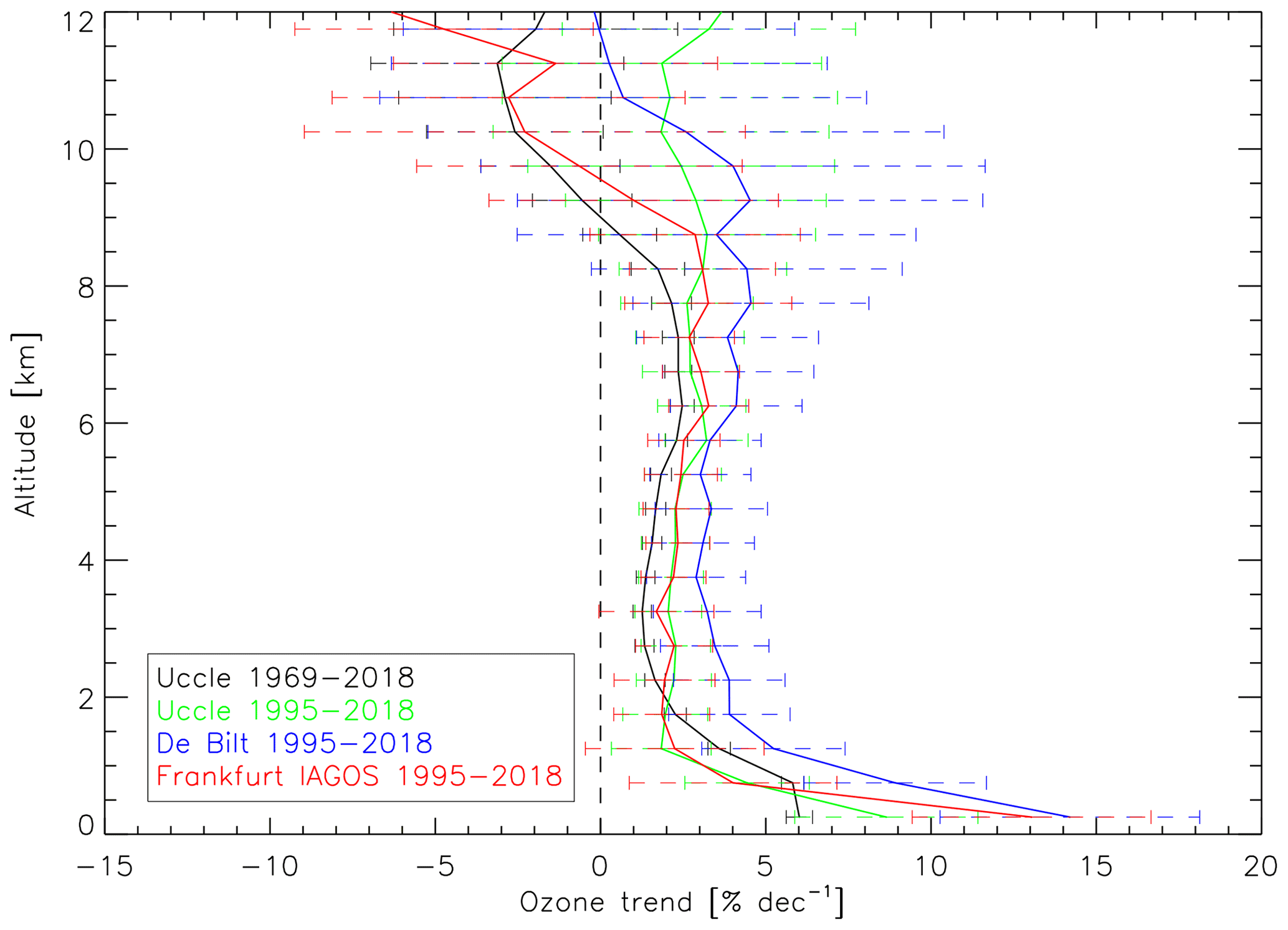
Figure 3Vertical distribution of trends in tropospheric ozone concentrations at Uccle for different periods, and at De Bilt (ozonesonde data) and Frankfurt (IAGOS data) for 1995–2018. Simple linear trends are calculated for monthly ozone anomalies in 1 km altitude ranges, and the error bars are 2σ standard deviations. The same colour coding is used as in Fig. 2: trends for the most recent Uccle sub-period (here 1995–2018) are in green; for the entire Uccle time series trends, we use black; and the De Bilt trends are shown in blue. The red line denotes the Frankfurt IAGOS trends in this figure.
Here, we calculated the tropospheric ozone trends from the Uccle and De Bilt ozonesonde time series and the MOZAIC (Measurement of Ozone and Water Vapour by Airbus in-service Aircraft) and IAGOS (In-service Aircraft for a Global Observing System) ascent and descent profiles at Frankfurt airport, about 320 km from Uccle. This MOZAIC-IAGOS dataset consists of more than 27 600 profiles, starting in August 1994, and is combined with the data from Munich airport, approximately 300 km southeast of Frankfurt, between 2002 and 2005 (about 4200 flights), to fill a large data gap in 2005 (also done in e.g. Petetin et al., 2016). With typical horizontal ozone correlation lengths of about 500 km in the troposphere (Liu et al., 2013), some correlation of especially free-tropospheric ozone trends between Uccle and Frankfurt and between Uccle and De Bilt is expected. We used simple linear trends based on the monthly anomalies at different altitude levels (see Fig. 3), as there is no consensus regarding which proxies should be used to account for natural variability. First, for the 1995–2018 period, the extremely good agreement between the Uccle (in green in Fig. 3) and IAGOS (in red) vertical ozone trends in the free troposphere (3–8 km) is striking. Although the integrated tropospheric ozone amounts for this altitude range are lower for the region above Frankfurt (14.9 DU) than above Uccle (16.2 DU), the overall relative trends are similar (2.09 ± 1.01 % per decade and 2.47 ± 1.01 % per decade respectively; see Fig. S7). The De Bilt trends (in blue in Fig. 3) are larger in the free troposphere and also have larger uncertainties due to the lower launch frequency. In this context, we mention the sensitivity analysis of IAGOS profiles above Europe by Chang et al. (2020), which concluded that an optimal sample frequency of 14 profiles per month is required to calculate trends with their integrated fit method (and about 18 profiles a month when this method is not used). Near the surface, the De Bilt trend is in better agreement with the Frankfurt trend, but the local surface ozone production and destruction and the boundary layer dynamics can vary substantially between the three sites considered here, so that the boundary ozone distribution and trends at the three sites are likely to be uncorrelated. However, comparing the lower tropospheric IAGOS measurements at Frankfurt with nearby (within 50–80 km) and more distant (within 500 km) surface stations, Petetin et al. (2018) showed that the IAGOS observations in the first few hundred metres above the surface at Frankfurt airport have a representativeness typical of suburban background stations (such as Uccle and De Bilt), and as one moves higher in altitude, the IAGOS observations shift towards a regional representativeness. A detailed description of the surface ozone trend at Uccle and its relation with ozone precursor trends is provided in Appendix B.
In the upper troposphere, the ozone concentration trends deviate more between the different datasets, both in magnitude and sign, with larger trend uncertainties. At these altitudes, the aircraft could be very distant from Frankfurt (or Munich) airport, as the ascent/descent profiles stop/start at about 400 to 500 km from the airport. Hence, the measurements at these altitudes represent large areas. Therefore, the closer agreement between the Uccle and De Bilt trends above 8 km compared with the IAGOS trend might also be attributed to a similar source region. Moreover, at these altitudes, the trends do not represent the tropospheric ozone temporal variability only, as the mean tropopause height ranges between 10.5 km (winter time) and 11.5 km (summer time), with standard deviations between 1 and 1.5 km, at both Uccle and De Bilt. As a consequence, lower stratospheric ozone concentrations will contribute to the estimated trends in the upper altitudinal levels of Fig. 3.
The Uccle tropospheric ozone concentrations have been increasing at about the same rate since 1969 (in black in Fig. 3) as they have since 1995 (in green in Fig. 3), and the post-2000 increase rate is also very similar (not shown here, but it is also suggested in the tropospheric ozone column time series shown in Fig. S7). The increase in (free) tropospheric ozone concentrations above Uccle until the early 2000s is consistent with the findings reported above (western) Europe in the literature review of Cooper et al. (2014). Over the 2000-2014 period, the emissions of the key ozone precursor, nitrogen oxides (NOx), declined in North America and Europe due to transportation and energy transformation (Hoesly et al., 2018). Therefore, the overall increase in ozone concentrations has flattened but has resulted in spatially and seasonally varying tropospheric ozone trends over North America and Europe, without consistency in even the sign of the ozone trends (Gaudel et al., 2018, and references therein). However, Cooper et al. (2020) concluded, based on the IAGOS observations, that the western Europe free-tropospheric trends since 1995 are predominantly positive. Using a different statistical approach, i.e. a nonlinear regression fit of a quadratic polynomial to normalized, deseasonalized monthly mean ozonesonde (merged data from Uccle, Hohenpeissenberg, and Payerne) and MOZAIC/IAGOS data (Frankfurt) between 3 and 4 km altitude, Parrish et al. (2020) indicated that those ozone concentrations increased through the 1990s, reached a maximum in the years 2001 (merged ozonesonde) and 2007 (IAGOS), and have since decreased.
To explain the tropospheric ozone concentration trends, Griffiths et al. (2020) used a chemistry climate model employing a stratosphere–troposphere chemistry scheme and found that, for the 1994–2010 period, despite a levelling-off of emissions, increased stratosphere-to-troposphere transport of recovering stratospheric ozone drives a small increase in the tropospheric ozone burden. Taking advantage of the high vertical resolution of the ozone profiles and the high frequency of launches at Uccle, we focus on the time variability of specific cases of deep intrusions of stratospheric air into the troposphere (i.e. tropopause folds). Akritidis et al. (2019) stressed the role of tropopause folding in stratosphere-to-troposphere transport (STT) processes under a changing climate, suggesting that tropopause folds will be associated with both the degree of ozone STT and inter-annual variability in ozone STT. Tropopause folds occur because of the ageostrophic circulation at the jet entrance and coincide with the frontal zone beneath the jet. The automatic algorithm applied in this work detects tropopause folds in the Uccle ozone-sounding profiles as ozone-rich (two criteria), stable (one criterion), and dry (one criterion) air mass layers located in an upper-level front in the vicinity of an upper-tropospheric jet stream (two criteria), and it is described in Van Haver et al. (1996). This identification by means of the above-mentioned six criteria is also illustrated in an example of an ozone sounding containing a tropopause fold in Fig. S8.

Figure 4(a) Relative frequency of detected tropopause folding events per year in the ozone soundings at Uccle. (b) Relative frequency of tropopause folding events per month.
Tropopause folds are rather rare events at Uccle: out of the 6526 soundings analysed for the 50-year period (1969–2018), only 290 soundings (or 4.4 %) showed evidence of a tropopause folding. However, similar occurrence rates (between 3 % and 10 %) have been found over Europe at French ozonesonde sites (Beekmann et al., 1997) and using other techniques (Rao et al., 2008; Antonescu et al., 2013). On a monthly scale, most folding events occur in March, June, July, and August (occurrence > 5 %), whereas in January, April, May, and December, the amount is lower (Fig. 4). Most important here within the context of the tropospheric ozone trends is the dramatic increase in the amount of tropopause folding events over time with a rate of 0.14 ± 0.02 % yr−1 (see also Fig. 4). Van Haver et al. (1996) detected a smaller and insignificant trend of 0.07 ± 0.11 % yr−1 at Uccle for the 1969–1994 period. On the one hand, the large increase over the entire time period might be explained by some technical aspects. Firstly, the higher vertical resolution of the sounding data in the more recent digital era (since 1990) might have an impact on the larger detected number of tropopause folds (thinner layers might be detected), although the number of events has continuously increased since then, at a slightly smaller annual rate of 0.12 ± 0.05 %. Secondly, a visual inspection of all profiles fulfilling at least five of the tropopause fold detection criteria led to a higher number of (manually) identified events (around 50 more), especially at the beginning of the time series. This is explained by the fact that the low humidity criterion was often not met in the automatic detection because there were no humidity data or the humidity sensor was iced (following the icing recognition algorithm of Leiterer et al., 2005). More recent types of radiosonde humidity sensors (in use since 2007 at Uccle) prevent ice contamination by heating the sensors during flight. However, this manual (and hence more subjective) mode of the algorithm still gives a 0.09 ± 0.02 % annual increase in the frequency of tropopause fold events since 1969. Therefore, we believe that the significant increase, although possibly overestimated by the automatic procedure, is nevertheless a robust feature of the analysis. Additionally, a higher rate of tropopause folding events is expected due to climate change (Tarasick et al., 2019, and references therein): climate change is projected to increase planetary wave activity inducing an accelerated Brewer–Dobson circulation. This acceleration, along with stratospheric ozone recovery, will lead to the increased transport of ozone from the stratosphere into the troposphere and, hence, more tropopause folding events. Akritidis et al. (2019) elaborated that the degree of increase in the downward transport of stratospheric ozone is partially driven by the long-term changes in tropopause fold activity.
To conclude, we found very consistent positive vertical tropospheric ozone trends between Uccle, De Bilt, and Frankfurt (IAGOS) since 1995, which are consistent with other studies, both observational studies and those using a modelling approach, but different processing and statistical methodologies can result in different European trend patterns for the last 2 decades.
Ozonesondes are virtually all-weather instruments (i.e. unaffected by clouds and precipitation) in contrast to most spectroscopic techniques, and they provide high vertical resolution ozone profiles from the ground to about 30 km. Therefore, satellite algorithms are based on ozonesonde climatologies and, in turn, satellites are validated by the sondes. Since the start of the ozone-measuring satellite era, ozone profiles from soundings at Uccle have been used for the validation of satellite ozone retrievals, e.g. the Stratospheric Aerosol and Gas Experiment (SAGE) II satellite profiles (Attmannspacher et al., 1989; De Muer et al., 1990). In this section, we give some recent examples of the application of the Uccle ozone profile data for operational satellite validation (Sect. 5.1) and for the scientific evaluation of both stratospheric (Sect. 5.2) and tropospheric (Sect. 5.3) ozone profile retrievals by satellite instruments. In these latter two sections, we also illustrate that a consistent and homogenous ozonesonde dataset, such as that from Uccle, is crucial to determine the long-term stability of (merged) satellite ozone retrievals.
5.1 Operational validation within EUMETSAT AC SAF
As partner of the European Organisation for the Exploitation of Meteorological Satellites (EUMETSAT) Atmospheric Composition Satellite Application Facilities (AC SAF), RMI is responsible for the validation of different ozone products (ozone profiles and (tropical) tropospheric ozone columns; see Hassinen et al., 2016; Valks et al., 2014; van Peet et al., 2014) from the Global Ozone Monitoring Experiment-2 (GOME-2) and Infrared Atmospheric Sounder Interferometer (IASI) instruments on board the MetOp A, B, and C satellite platforms. These different instruments give the opportunity to obtain a unique dataset, retrieved with an identical technique, from the beginning of the MetOp-A/GOME-2 instrument in 2007 until the phase-out of the third instrument (MetOp-C/GOME-2), which is officially foreseen in 2022. GOME-2 ozone profiles are given as partial ozone columns, expressed in Dobson units, on 40 varying pressure levels between the surface level and 0.001 hPa and are calculated by the Ozone Profile Retrieval Algorithm (OPERA; van Peet et al., 2014). The a priori information used for the retrieval is obtained from McPeters and Labow (2012).
For the validation of GOME-2 ozone profiles within the AC SAF, ozonesonde measurements are extensively used. However, for a meaningful comparison, the ozonesonde profiles need to be integrated first between the GOME-2 pressure levels. When comparing a single ozonesonde profile with different GOME-2 profiles, the actual reference ozone values are not identical due to the fact that the GOME-2 vertical levels vary from one measurement to another. GOME-2 has a nominal spatial resolution of 80 km × 40 km, but for the shortest UV wavelengths, the integration time takes 8 times longer because of the lower number of photons arriving on the detector pixels. Furthermore, as the ozonesondes and the satellite do not have the same vertical resolution, it is necessary to consider the averaging kernels (AVK) in order to “smooth” the ozone soundings towards the resolution of the satellite (Rodgers, 2000).
In Fig. 5, the relative differences between the MetOp-A operational ozone profile product and the Uccle ozonesonde profiles are shown for the year 2018 (in red). The following co-location criteria were applied: a geographic distance of less than 100 km between the GOME-2 pixel centre and the sounding station location, and a time difference of less than 10 h between the pixel sensing and the sounding launch time. The figure highlights two different aspects of the operational validation. Firstly, it can be noted that applying the averaging kernels to the sounding profiles improves the comparison with the GOME-2 ozone product significantly (i.e. by 15 %), in particular in the lower stratosphere (compare the full lines with dashed lines in Fig. 5). The lower stratosphere is the region with the highest ozone variability, so smoothing the high-resolution ozonesonde profiles to the GOME-2 vertical resolution will have the largest effect here by removing details of the differences. Secondly, as the GOME-2 ozone profile product is based on UV measurements, it is sensitive to degradation of the UV sensor (van Peet et al., 2014; Munro et al., 2016). For example, the measured values of the GOME-2A irradiance in the UV (below 300 nm) had decreased by roughly 80 % in 2016 (since its launch in 2007). As the vertical ozone profile retrieval algorithm depends on an absolute calibrated reflectance (sun-normalized radiance), there is a need to correct for this temporal change of the (joint) radiance and irradiance. This method depends on the assumption that, taken as an average across the globe, the atmospheric constituents (mainly ozone) will be close to the multi-year climatological value from McPeters and Labow (2012). The climatological ozone profile is then scaled with the assimilated total ozone columns to get the overall ozone absorption correct (Tuinder et al., 2019). This degradation correction has been applied to the data for the relative differences with the Uccle data in Fig. 5 (in grey). From this figure, it should be clear that this degradation correction significantly improves the agreement with the Uccle ozonesonde data compared with the operational product (in red), resulting in relative differences between GOME-2 ozone profiles and the Uccle data within the target error range of 15 % (marked by the vertical red lines). The improvement after degradation correction is a promising result, showing the challenge for UV–VIS sounders to obtain a stable ozone profile product on different sensors (GOME-2A, 2B, and 2C) for different periods using the same type of optical instrument. More feedback on the status of the operational EUMETSAT product can be obtained in the validation reports, which are available on the AC SAF website (https://acsaf.org, last access: 29 May 2020; e.g. Delcloo and Kreher, 2013).

Figure 5Relative mean differences and standard deviations between ozone profiles retrieved from MetOp-A/GOME-2 and Uccle ozone profiles for the time period from January to December 2018. The red graph represents the mean differences when using the operational MetOp-A/GOME-2 product, and the grey graph represents the mean differences when the UV sensor degradation correction has been applied in the MetOp-A/GOME-2 ozone retrieval. The relative mean differences denoted by dashed lines are obtained after applying the averaging kernel to the Uccle sounding data. Finally, the thin red vertical lines mark the ±15 % target error range of the MetOp-A/GOME-2 ozone profile product.
5.2 Validation of Aura-MLS stratospheric ozone profiles
The Microwave Limb Sounder (MLS; Froidevaux et al., 2008) is one of the four instruments on the Earth Observing System (EOS) Aura satellite. MLS has been measuring vertical profiles of atmospheric trace gases (including ozone), temperature, geopotential height, relative humidity, cloud ice water content, and cloud ice water path, since its launch in 2004. Global measurements (from 82∘ S to 82∘ N), in a near-polar, sun-synchronous orbit, at two fixed solar times, noon–night, at around 01:30/13:30 LST (local solar time) are achieved, with the number of profiles over, for example, ozonesonde sites varying between zero and six daily. MLS products have been validated to be very accurate and stable (Jiang et al., 2007; Froidevaux et al., 2008) and have been used in many studies involving ozonesonde measurements (e.g. Witte et al., 2017; Stauffer et al., 2020). Here, we have implemented the MLS v4.2 data, screened according to the v4.2 Level 2 MLS Data Quality document (Livesey et al., 2020), and have compared the satellite overpass measurements with coincident ozonesonde profiles at Uccle. Because there are multiple profiles crossing over Uccle at a fixed time, the profile closest in distance is used for the validation. Both the noon and night overpasses have been used, as we did not find significant differences between them. As a result, ∼ 3000 profiles were included into the validation. Thanks to the relatively dense and regular MLS vertical resolution of around 2.5 km in the 10–200 hPa pressure range, it is feasible to interpolate the Uccle ozonesonde data to the MLS pressure levels on a fine pressure grid of 2.5 km. Applying the time invariant MLS averaging kernel on the latitude of Uccle on the ozonesonde data did not have a large effect on the smoothing of the vertical ozonesonde profile, compared with applying the identify matrix to the ozonesonde vertical profile (< 1 %). This contrasts strongly with the GOME-2 and TES retrievals (see Sect. 5.3), where the spatio-temporal varying averaging kernels affect the vertical ozone profiles substantially and, as such, should be used on the sonde data for pairwise comparison. The mean annual relative differences between MLS and Uccle ozonesondes are shown in Fig. 6. Different conclusions can be drawn from this figure. First, MLS and the Uccle ozonesondes compare very well, within ±5 % between 10 and 70 hPa (grey shading in Fig. 6). At pressures lower than 10 hPa, ozonesonde measurements systematically underestimate ozone due to the evaporation or freezing of the sensing solutions (see also the composite ECC-MLS in Fig. 3 in Stauffer et al., 2020), and they have a larger uncertainty due to increased pump efficiency uncertainty at low pressures. On the other hand, at pressures larger than 70 hPa, the MLS ozone retrieval is more challenging because of the longer atmospheric path and the lower ozone volume mixing ratios increasing the relative differences. Another important finding from this figure is that the mean annual relative differences are very consistent over the different years, which means that both the MLS instrument and the Uccle ozonesonde time series are very stable with respect to one another. In addition to this, we also want to mention that the relative differences between the MLS and Uccle ozonesondes are very similar for the different seasons (see Fig. S9).
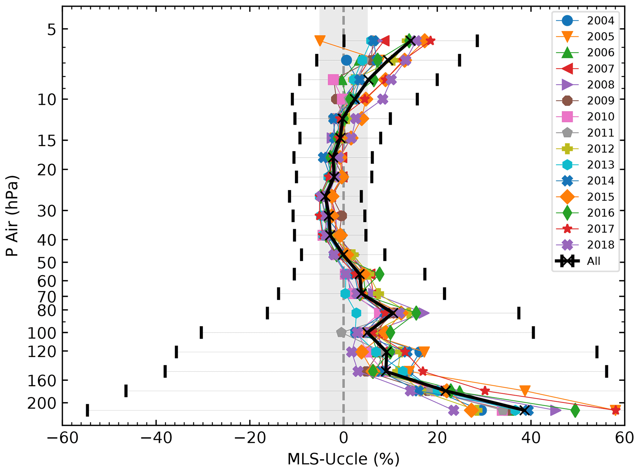
Figure 6Relative ozone profile differences between the MLS and Uccle ozonesondes. The different colours correspond to the different yearly averages, illustrating the large consistency among them. The black line represents the overall mean relative difference, and the error bars show ±1 standard deviation due to the individual differences. Note that individual differences are relatively large at some pressure levels, but they are cancelled out in the yearly mean.
5.3 Validation of Aura-TES tropospheric ozone profiles
Here, we compare the tropospheric vertical ozone profiles of the Uccle sondes coinciding with the observations from the Tropospheric Emission Spectrometer (TES) sensor on-board the Aura satellite for the period from late 2004 to early 2018, when the instrument was decommissioned. TES is an infrared Fourier transform spectrometer (Beer et al., 2001; Beer, 2006) that measures radiance spectra of Earth's atmosphere, predominantly nadir-viewing, at wavelengths between 3.3 and 15.4 µm. The nadir vertical profiles are spaced 1.6∘ apart along the orbit track and have a footprint of approximately 5 × 8 km2 (Beer et al., 2001; Beer, 2006).
The vertical sensitivity of the TES-retrieved ozone is the largest for the troposphere, with a vertical resolution for ozone profiles of 6–7 km, corresponding to 1–2 degrees of freedom in the troposphere (Jourdain et al., 2007). Prior to applying TES ozone data, they are subject to screening, using the TES ozone master quality flag that accounts for clouds and an overly large difference between observed and simulated radiances (Osterman et al., 2008).
As in Nassar et al. (2008) and Verstraeten et al. (2013), we apply temporal and spatial coincidence criteria of ±9 h and ±300 km respectively between the sonde and TES observations. These criteria can provide enough profiles for a statistically meaningful comparison while also being strict enough to ensure a high probability that both instruments sample similar air masses. A mapping matrix is used to interpolate the sonde data to the 67-level pressure grid (from 1212 to 0.1 hPa) used in the TES retrievals. The TES averaging kernel was then applied to the 67-level pressure grid of the Uccle sonde data to ensure a consistent comparison between TES and ozonesonde data, excluding the influence of the a priori ozone profile needed to regulate the TES retrieval (Verstraeten et al., 2013).
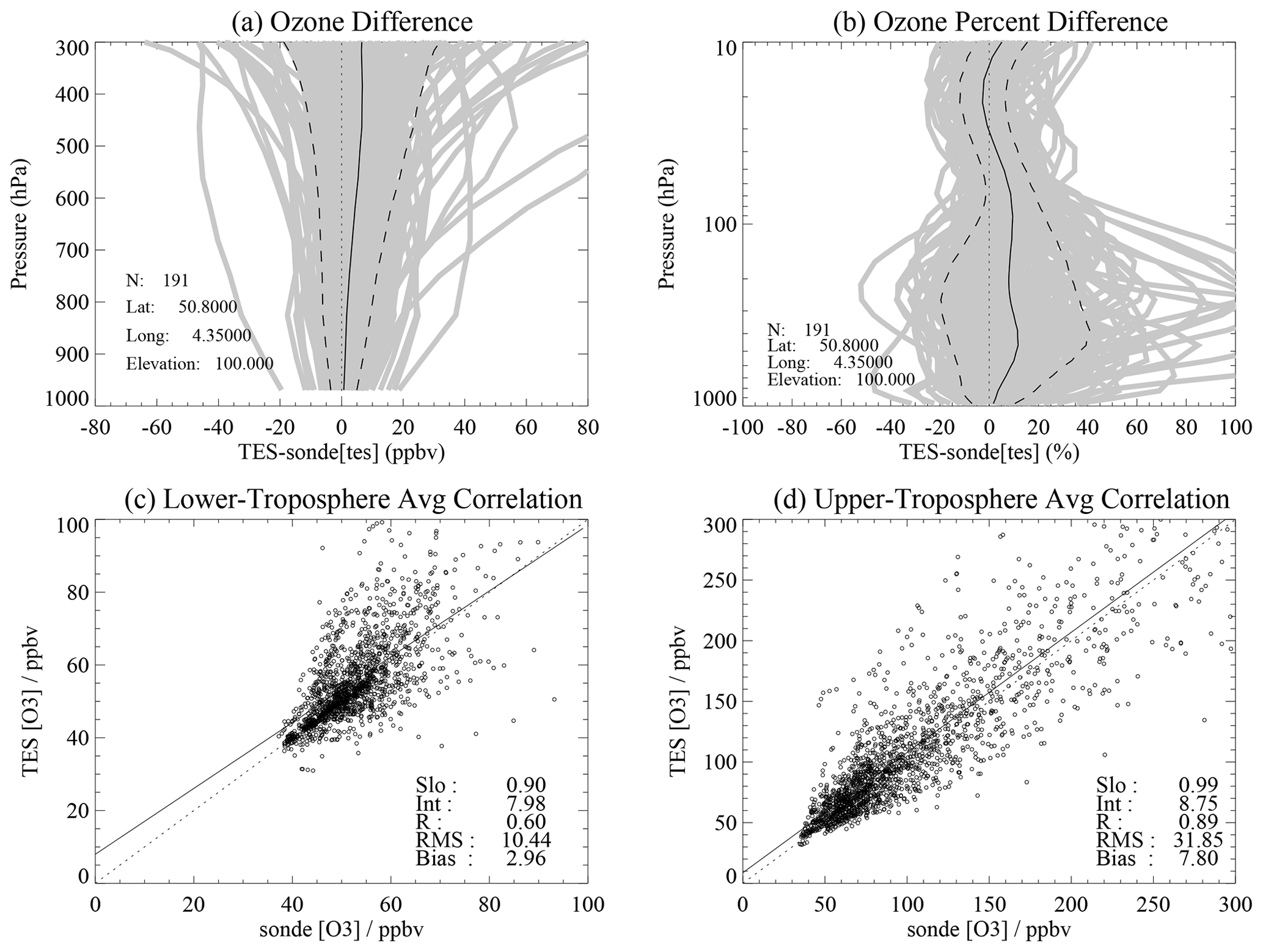
Figure 7Absolute TES–sonde tropospheric ozone vertical differences (a) and relative differences (b) for the whole profile of Uccle. Individual difference profiles are shown in grey; the mean difference and 1 standard deviation profiles are shown in black. N is the number of valid profiles after flagging TES data and using the maximum 300 km and 9 h coinciding criteria. Panel (c) illustrates the correlation between TES and sonde O3 for the lower troposphere (1000 to 500 hPa), including the slope (Slo), intercept (Int), and correlation (R) of the linear regression; the root mean square error (RMS); and the bias. Panel (d) is the same as panel (c) but for the upper troposphere (500 hPa to the tropopause).
By applying all these constraints (coinciding criteria and the TES ozone master flag), 191 suitable coincidences or data pairs for the full time range from 2004 to 2018 were collected. Figure 7a and b present TES–sonde tropospheric ozone profile differences for the Uccle sondes. Figure 7a shows the absolute ozone vertical profile differences (TES–sonde) in the troposphere (1000–300 hPa), and Fig. 7b shows the relative differences ((TES − sonde) × 100 sonde) for the full vertical ozone profile (1000–1 hPa).
Figure 7 indicates that TES is generally positively biased within the troposphere by up to ∼ 10 ppbv, corresponding to relative differences of up to ∼ 15 %. The TES bias varies slightly as a function of pressure. TES appears to be almost unbiased with respect to the sondes in the lower troposphere, but this actually reflects the insensitivity of TES to ozone in the lower atmosphere for situations with a lower brightness temperature, as encountered at higher latitudes. As the TES signal in the troposphere has typically 1–2 degrees of freedom, analysing the TES bias for two vertical regimes – the lower troposphere (LT; 1000 to 500 hPa) and the upper troposphere (UT; 500 hPa to tropopause) – might be meaningful (Nassar et al., 2008). From a linear regression of all TES versus sonde ozone data pairs for Uccle in the lower troposphere (Fig. 7c), we find a slope of 0.90 with an intercept of 7.98 (R = 0.60) and a bias of +2.96 ppbv. For the upper troposphere (Fig. 7d), the bias is a bit higher (7.80 ppbv), the correlation (R) is 0.89, and the slope and intercept are 0.99 and 8.75 respectively. These values are in line with reported values for data pairs collected for the whole northern mid-latitude region (Verstraeten et al., 2013).
The temporal stability of the TES sensor for tropospheric ozone can be assessed by applying the Theil–Sen trend statistics (Theil 1950a, b, c; Sen, 1968) on the time series of the TES–sonde data pairs for each pressure level in the troposphere (surface to 300 hPa). Analysis shows that all p values are larger than 0.05, indicating that all slopes of the linear regression are not statistically different from zero in the troposphere. All R2 values are smaller than 0.01. Thus, there is no reason to assume any temporal trend for data pairs in the troposphere. This is in line with the same analysis for the 464 hPa level by Verstraeten et al. (2013).
Having started operationally in 1969 with the aim of using ozone as a tracer to study the general air circulation in the troposphere and the lower stratosphere, the high-frequency (three times a week) mid-latitude Uccle ozone-sounding time series now extends over more than 50 years, covering over 7000 profiles. Over this entire period, attention has always been paid to the consistency of the time series, resulting in only one major change: the switch from BM to En-Sci ECC sondes in 1997. However, this change was well documented with dual launches and pump efficiency laboratory measurements of both pump types, so that a unique correction method for both sonde types, a PRESsure and Temperature dependent total Ozone normalization (PRESTO; Van Malderen et al., 2016), has been developed (De Backer et al., 1998a, b) to guarantee the data homogeneity. Another distinct feature of the Uccle ozonesonde dataset is the correction for urban SO2 interference with the chemical reactions in the ozone cells in the first half of the period.
Although satellites provide global routine measurements of ozone profiles with increasing accuracy and spatial resolution, ozonesondes are the only technique that has been able to provide (for the last 50 years) accurate (around 5 %–10 %), vertically resolved observations from the surface up to the lower stratosphere, unaffected by clouds or precipitation. Furthermore, they can resolve strong gradients in the UTLS (upper troposphere–lower stratosphere) while precisely locating the thermal tropopause (Thompson et al., 2011). In this paper, we illustrated the importance of the Uccle ozonesonde dataset in two specific application areas: for the assessment of the long-term vertical ozone trends and for the validation of satellite retrievals of ozone profiles. The strength of the ozonesonde measurements (and the Uccle time series in particular) specifically lies in the combination of these two aspects of ozone research, along with their applicability in process studies. The major conclusions are summarized in the following.
Making use of the LOTUS multiple linear regression model including the QBO, the solar radio flux, ENSO, and AOD as explanatory variables, we found that the stratospheric ozone concentrations at Uccle have declined at a significant rate of around 2 % per decade since 1969. This overall decline can mainly be attributed to the increasing ODS emissions, with a rather consistent rate of decline of around −4 % per decade for the 1969–1996 period. Since 2000, a recovery of between +1 % per decade and 3 % per decade of the stratospheric ozone levels above Uccle has been observed, although this is not significant and is not for the upper stratospheric levels measured by ozonesondes. Hence, the significant decline in lower stratospheric ozone amounts since 1998, as reported by Ball et al. (2018, 2019), is not present in the Uccle and nearby De Bilt time series. For the considered periods, we found an overall agreement between the sign of the stratospheric temperature trends and those ozone concentration trends (i.e. a cooling of the stratosphere in 1969–2018 and 1969–1996 and an insignificant warming for all but the lower stratospheric layers since 2000), underlining the possible mutual interaction between the stratospheric ozone concentration and temperature changes.
In Appendix A, we show that the total column ozone loss at Uccle between 1971 and 1996 (at a rate of −1.6 % per decade) has nearly fully recovered due to the +1.9 % per decade gain since 2000. In the light of the discussion on the stratospheric ozone trends in the previous paragraph, this would mean that the tropospheric ozone amounts at Uccle should increase from the mid-1990s. We indeed confirmed a very consistent increase in the ozone concentrations of 2 % per decade to 3 % per decade throughout the entire free troposphere, a number which is in almost perfect agreement with the trends derived from the IAGOS ascent/descent profiles at Frankfurt and is 1 % per decade lower than the De Bilt tropospheric ozone trends. The Uccle 1995–2019 trend is even 0.5 % per decade to 1 % per decade higher than the 1969–2019 trend. Despite the levelling-off of tropospheric ozone precursor emissions, the tropospheric ozone amounts in Uccle are still increasing. Based on chemistry climate model calculations, Griffiths et al. (2020) found that an increase in the tropospheric ozone burden might be driven by increased stratosphere-to-troposphere transport of recovering stratospheric ozone. It should also be noted that the number of tropopause folding events in the Uccle time series increased significantly over time, which might be an indicator of increased transport of ozone from the stratosphere into the troposphere. However, in line with the free-tropospheric ozone, the surface ozone concentrations at Uccle have continued to increase since the beginning of those measurements in the 1980s, despite the decreasing on-site concentrations of precursor trace gases such as CO, NO, and NO2 (see Appendix B).
For the operational validation of the GOME-2 and IASI ozone profiles within the EUMETSAT AC SAF, the role of ozonesonde profiles is crucial. We showed how the Uccle dataset can be used to evaluate the performance of a degradation correction for the GOME-2 UV sensors. The Uccle ozonesondes are also used to assess the accuracy and stability of satellite ozone retrievals. Here, we showed that the Aura-MLS overpass ozone profiles agree very well with the ozonesonde profiles, within ±5 % between 10 and 70 hPa. Another instrument on the same Aura satellite platform, TES, has its largest vertical sensitivity for ozone in the troposphere, and it is generally positively biased with respect to the Uccle ozonesondes in the troposphere by up to ∼ 10 ppbv, corresponding to relative differences of up to ∼ 15 %. Using the Uccle ozonesonde data series as a reference, we also found that the temporal stability of both satellite retrievals is excellent. Inversely, satellite total ozone retrievals and MLS have enabled the detection of a post-2013 drop-off in total ozone at a third of global ozonesonde stations (Stauffer et al., 2020), a number now reduced to about 20 % (12 of 60 global stations; Ryan Stauffer, personal communication, 2021). Our analysis with MLS confirmed the above-mentioned previous finding that Uccle is not affected by any total column drop-off of more than 3 % in its time series.
A higher flexibility of ozonesonde launch times toward satellite overpass times is an emerging issue that needs to be considered against the preference for a fixed launch time for, for example, the assessment of tropospheric ozone trends. Moreover, for over a decade, weather prediction centres have been incorporating chemistry into operational forecasts that assimilate satellite ozone retrievals, and ozonesondes have been used for the external evaluation of those model forecasts (e.g. for tropospheric ozone; Flemming et al., 2015), analyses (e.g. for stratospheric ozone; Lefever et al., 2015), and reanalyses (e.g. Inness et al., 2019). Those services require near-real-time delivery of the ozonesonde measurements, with an operational quality assessment/quality control tool. These are the challenges facing operational applications of ozonesondes. For the assessment of the long-term variability of ozone concentrations at different atmospheric altitudes and the interaction between climate change and ozone (also studied in coupled chemistry climate and chemistry transport models; see e.g. Morgenstern et al., 2017), the availability of a long-term homogeneous dataset is crucial. Homogenization efforts of ozonesonde networks and/or datasets (Tarasick et al., 2016; Van Malderen et al., 2016; Thompson et al., 2017; Witte et al., 2017, 2018, 2019; Sterling et al., 2018) should, therefore, be continued and extended. With these developments in mind, we aim at continuing the pioneering role that the Uccle time series has had in some research areas during its 50-year lifetime.
The total column ozone amounts at Uccle, which have been available since 1971, are retrieved with a Dobson UV spectrophotometer (no. 40, 1971–1989), a single-Brewer UV spectrophotometer (no. 16, 1990–current, but used in the time series until the end of 2001), and a double-Brewer UV spectrophotometer (no. 178, 2002–current). The calibration history of the Dobson instrument is documented in De Muer and De Backer (1992), and the transition to the Brewer instrument is described in De Backer and De Muer (1991). Both Brewer instruments were recalibrated against the travelling standard Brewer instrument no. 17 in 1994 (no. 16 only), 2003, 2006, 2008, and against the travelling reference Brewer no. 158 since 2010 every second year. The stability of the instruments is also continuously checked against the co-located instruments (with the Dobson no. 40 from 1991 until May 2009 and between both Brewers since 2001). Internal lamp tests are performed on a regular basis to check whether a Brewer instrument is drifting. When instrumental drift is detected, it is corrected for.
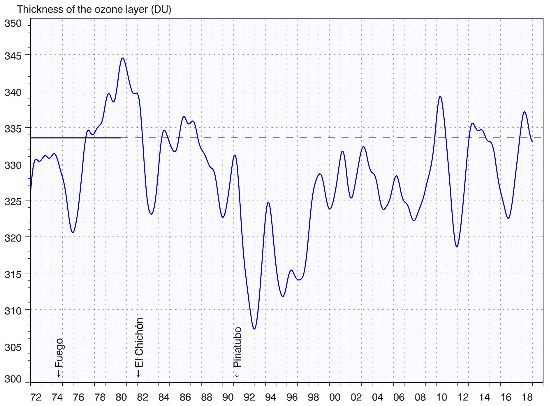
Figure A1Evolution of the total ozone column at Uccle as observed with Dobson D40 (1972–1989), Brewer no. 16 (1990–2001), and Brewer no. 178 (2002–present). The solid horizontal black line marks the 1972–1980 total ozone average (period before catalytic ozone loss), extended until the end of the time series by the dashed horizontal line. The periods of major volcanic eruptions affecting the ozone layer are indicated on the time axis as well.
The time series of total ozone measurements is shown in Fig. A1 but has been smoothed by applying a low-pass Gaussian filter with a width at half height of 12 months in order to filter out variations with frequencies higher than 1 year. With this representation, the impact of the major (strato)volcanic eruptions of Fuego (Guatemala, October 1974), El Chichón (Mexico, March/April 1982), and Pinatubo (the Philippines, June 1991) is shown in the significant dips in Uccle total ozone. Indeed, the episodes of enhanced stratospheric aerosol-related ozone loss after those major volcanic eruptions are confirmed by model results (see e.g. Tie and Brasseur, 1995; Solomon, 1999; and Aquila et al., 2013, for a description of the mechanism behind this) and can clearly be identified in the time series. Also the other inter-annual variability in Fig. A1 is very similar to the Northern Hemisphere (NH) annual mean total ozone time series of five bias-corrected merged datasets in the 35–60∘ N latitude band in Weber et al. (2018; their Fig. 2). In 2010, the Uccle ozone levels were unusually high, which was the case over the entire NH extratropics. An unusually pronounced and persistent negative phase of the Arctic Oscillation and North Atlantic Oscillation in 2010 with the coincidence of the northern winter 2009/2010 and the easterly wind-shear phase of the QBO have been identified as major contributors (Steinbrecht et al., 2011) of this excess ozone. The 2011 ozone low anomaly cannot be fully explained by including this Arctic Oscillation and other dynamical proxies (e.g. for the Brewer–Dobson circulation) in the multiple linear regression model used in Weber et al. (2018), but it might be linked to the strong Arctic ozone loss in 2011 (Manney et al., 2011). The below-average annual mean Uccle and NH total ozone in 2016 is partly ascribed to the severe Arctic ozone depletion in the same year and is related to the anomalous meridional circulation changes induced by the Quasi-biennial Oscillation (QBO) (see references in Weber et al., 2018).
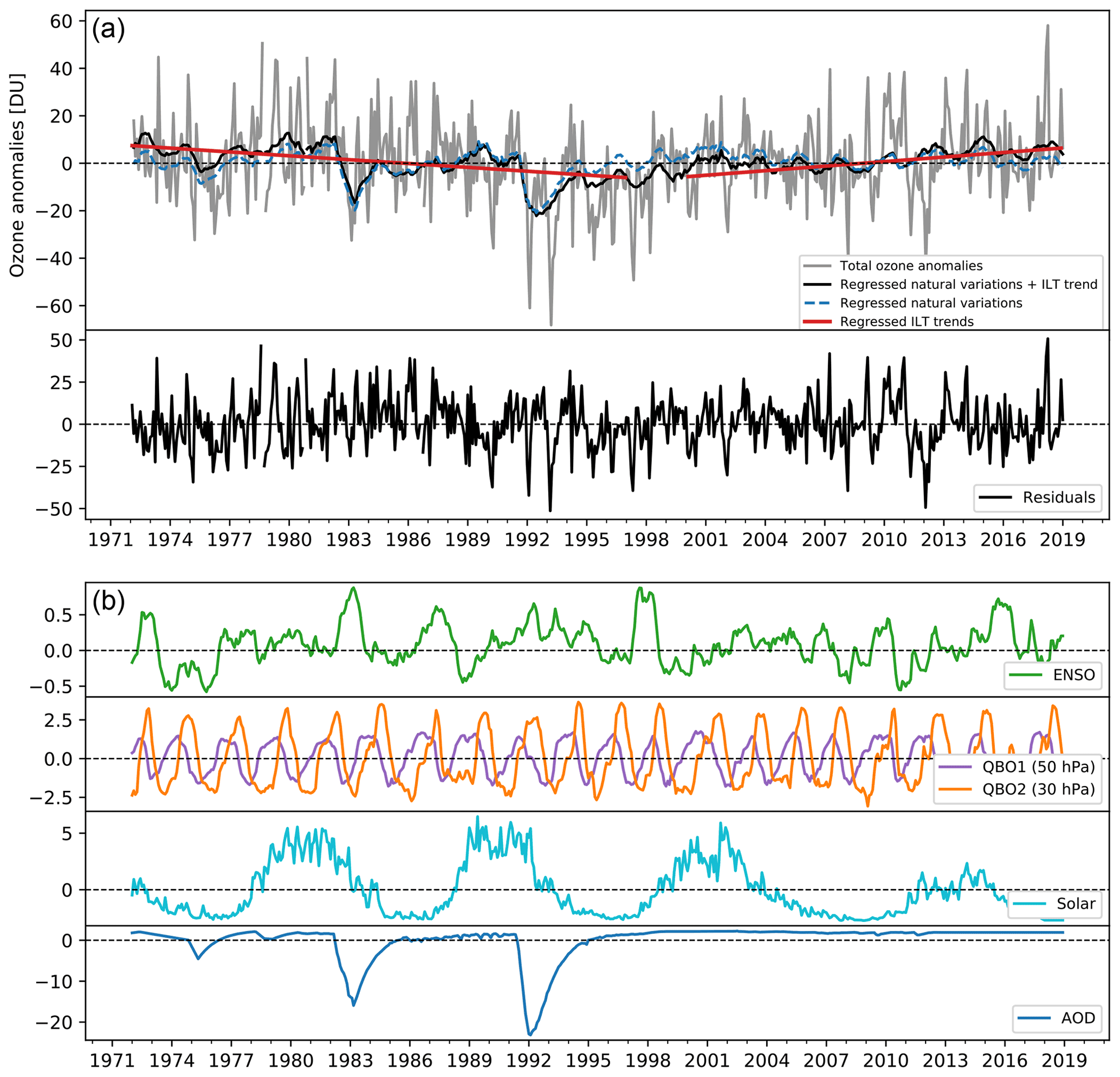
Figure A2Terms in the LOTUS multiple linear regression model for the Uccle total ozone amounts. Panel (a) shows the observed total ozone monthly anomalies in grey. The black line is the result of the full LOTUS regression model including the independent linear trends (ILTs, thick red lines). The pre-1997 trend equals −1.6 ± 0.5 % per decade, and the post-2000 trend equals +1.9 ± 0.8 % per decade. The dashed blue line shows the sum of the terms of the LOTUS model without the ILTs included. The bottom of panel (a) shows the residuals in the observed ozone concentrations with the full LOTUS model subtracted. Panel (b) shows the contributions (from top to bottom) of ENSO, QBO, the solar cycle, and aerosols to the reconstructed time series (blue dashed line) in panel (a).
To study the long-term temporal variability of the total ozone amounts at Uccle, we make use of the LOTUS MLR regression model that we also applied to estimate the stratospheric vertical ozone trends in Sect. 4.1. The model fit and the different contributors are shown in Fig. A2. The inter-annual variability is reasonably captured by this model, although this MLR is not able to model the large excursions in some years (e.g. 2011–2012) without the use of some additional terms accounting for the Arctic Oscillation or the Brewer–Dobson circulation (Weber et al., 2018). As can be noted from the observation-model residuals, the long-term temporal variability is well described by the two independent linear trends. Before 1997, ozone declined at Uccle at a rate of −1.6 ± 0.5 % per decade due to the anthropogenic production of ozone-depleting substances (ODS), transported into the stratosphere, with peak concentrations in 1997. This decline rate is comparable to the NH mid-latitude value of −2 % per decade to −3 % per decade (Weber et al., 2018; WMO, 2018), especially considering that the Uccle total ozone time series starts earlier than the satellite total ozone time series used in those assessments (from 1979). Subsequently, from 2000 onwards, the total ozone increased again at a rate of +1.9 ± 0.8 % per decade at Uccle. This ozone recovery estimate is significantly larger than the NH mid-latitude trend of +0.2 % per decade to +0.5 % per decade (Weber et al., 2018; WMO, 2018) and even larger than the expected NH trends from equivalent effective stratospheric chlorine (EESC) changes, which are about +1 % per decade (WMO, 2018). At Uccle, the total ozone amount seems to have almost fully recovered, as could also be noted by looking at the monthly anomaly time series in Fig. A2. Because the Dobson and Brewer spectrometers are calibrated regularly (see above), we have no doubts regarding the homogeneity of the time series. In general, according to Weber et al. (2018), the ozone increase after 2000 is not only due to the (slow) decrease in ODSs in the stratosphere but also because of atmospheric dynamics, notably ozone transport via the strengthening Brewer–Dobson circulation. At Uccle, the strongest ozone increase since the beginning of this century has taken place in late winter–early spring (February–April), at a rate of 3 % per decade to 4 % per decade, while the ozone transport by the Brewer–Dobson circulation from its tropical source region poleward and downward into the lower stratosphere has been strongest during wintertime (e.g. Butchart, 2014; Langematz, 2019).
While total ozone seems to have nearly fully recovered at Uccle, the stratospheric ozone amounts have not (see Figs. 2 and S5 for the monthly anomaly time series of the ozone concentrations in a layer 10 km above the tropopause height). The stratospheric ozone concentrations decreased between 1969 and 1996 at a rather consistent rate of around −4 % per decade (between 5 and 20 km above the tropopause), which was, therefore, larger than the total rate of ozone decline. Since 2000, a recovery of between +1 % per decade and +3 % per decade of the stratospheric ozone levels above Uccle has been observed, although it has not been significant and has not been for the upper stratospheric levels measured by ozonesondes. This value is comparable to the total ozone recovery rate at Uccle. To reconcile the stratospheric ozone trends from the ozonesondes with the total ozone trends at Uccle1, it should also be noted that, throughout the entire free troposphere (contributing for about 10 % to the total ozone amount), a very consistent increase in the ozone concentrations of +2 % per decade to +3 % per decade is measured since both 1969 and 1995 (see Fig. 3).
In this appendix, we elaborate more on how representative and complementary the surface ozone trend derived from the ozonesonde data at Uccle is compared with that from a surface monitoring station at the same site. The ground network of (air quality) stations provides surface ozone measurements at higher temporal and horizontal resolution and with higher accuracy than ozonesonde measurements, but these latter measurements also provide vertical ozone profiles in the lower troposphere and sometimes even over a longer time span. As a matter of fact, the ozonesonde launch site at the urban background site Uccle has also hosted surface measurements of ozone since 1986, performed by the Brussels Environment Agency. From the surface measurements, we consider the (30 min averaged) values at 11:30 UT, closest to the ozonesonde launch time. The monthly mean time series of those surface measurements are shown in Fig. B1, along with the lowest 1 km mean ozone measurements derived from the ozonesondes. The agreement between the surface ozone measurements from both devices is, in terms of monthly means, excellent, apart from a more or less constant offset. This offset might be explained by the difference in air masses for which the ozone concentrations are measured (surface versus surface to 1 km above the ground) as well as by the Uccle pre-launch procedure of testing the ozonesonde–interface–radiosonde configuration by exposing the ozonesonde to (stratospheric) ozone concentrations for a short time (< 30s) between 15 and 30 min prior to launch. Because of the slow time constant of 20–25 min in the chemical reactions in the cell, this pre-launch ozone exposure might still contribute to the measured cell current immediately after launch, resulting in a positive bias in the boundary layer ozone measurements with the ozonesondes.
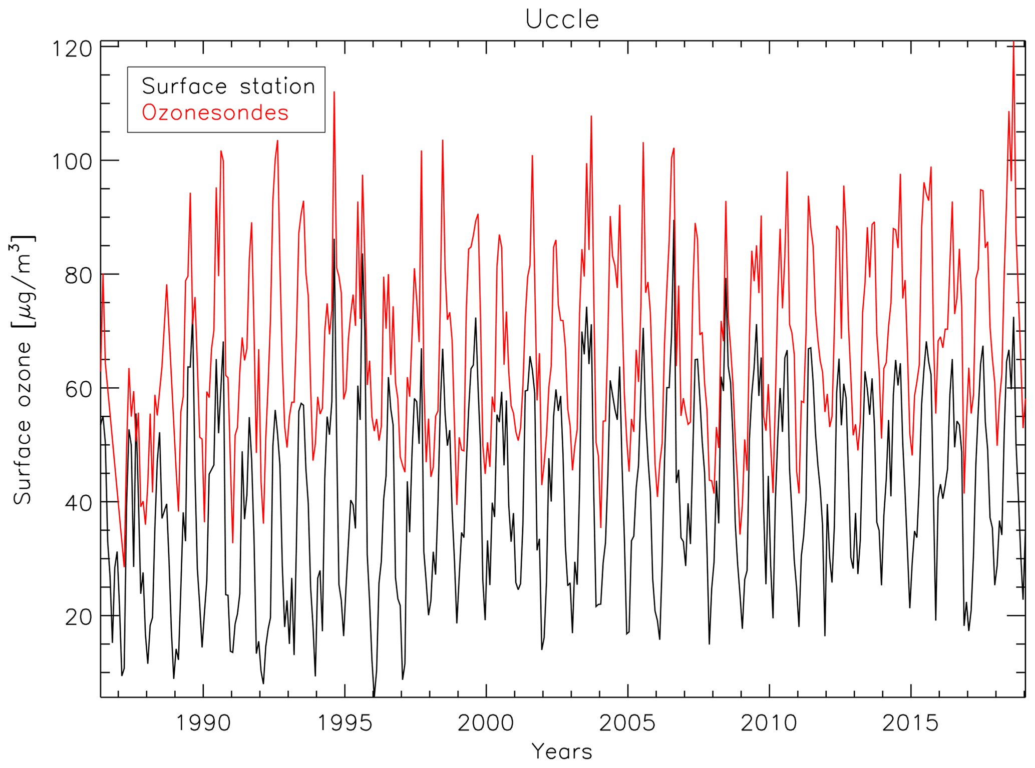
Figure B1Monthly mean time series of Uccle surface ozone (black) from the air quality monitoring station and mean ozone in the lowest 1 km above Uccle from the ozonesonde launches (red).
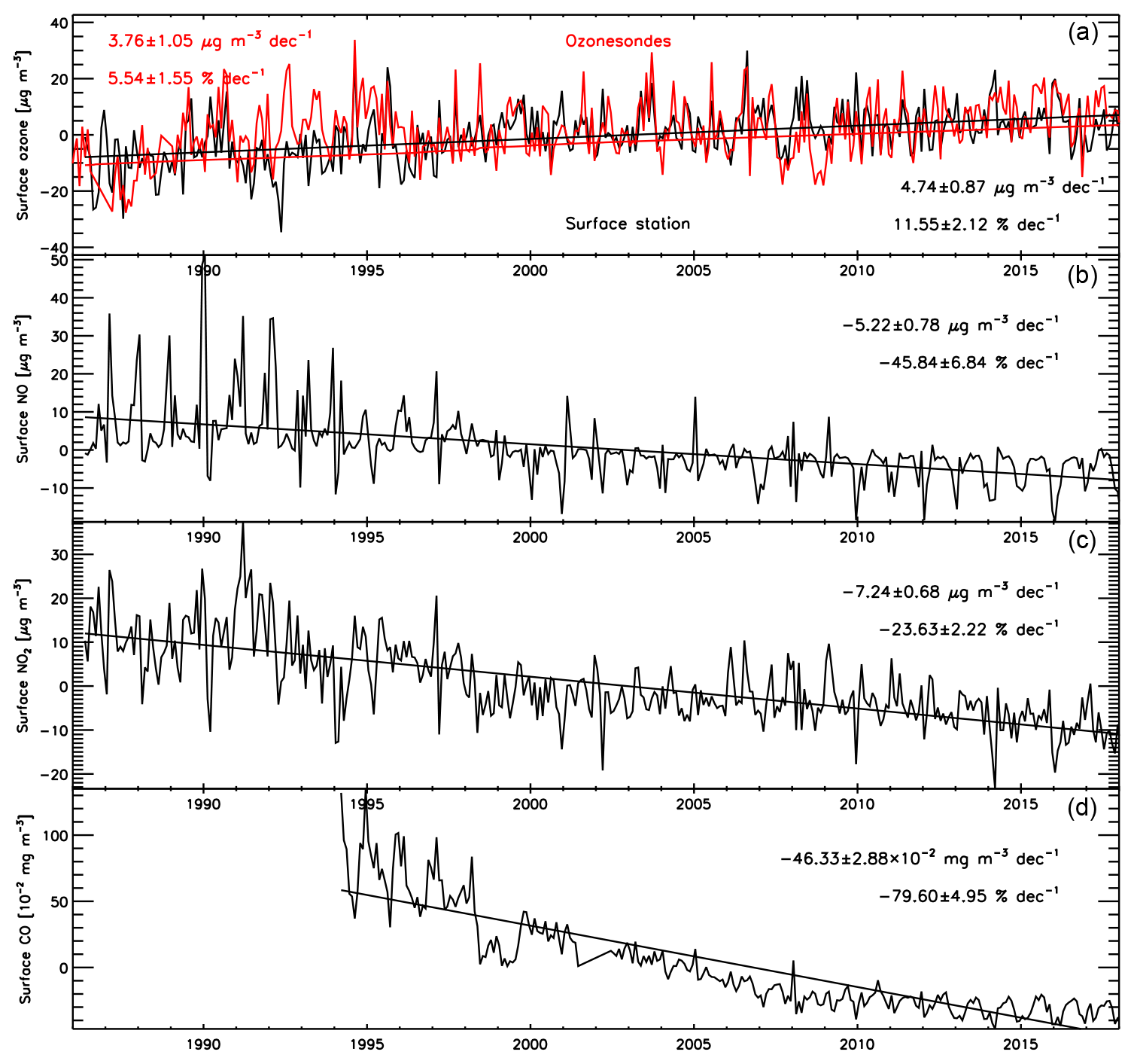
Figure B2Monthly anomaly time series of Uccle surface ozone (a, black) and mean ozone in the lowest 1 km above Uccle from the ozonesonde launches (a, red) and ozone precursor measurements at Uccle (NO, NO2) and Elsene (CO, 5 km from Uccle). Linear trends are shown along with the absolute and relative trend estimates and their 2σ uncertainties.
Both time series reveal a statistically significant (according to a Spearman test; see e.g. Lanzante, 1996) increase in surface ozone concentrations since 1986 (see Fig. B2), with a trend value 25 % higher for the surface ozone measurements compared with the sonde's measurements from the lowest 1 km (0.47 versus 0.38 µg m−3 yr−1 in absolute terms). Uccle is a suburban site; thus, its increase in the mean surface ozone concentrations is in line with the findings from Yan et al. (2018) over European suburban and urban stations during the 1995–2012 period2, with trends between 0.20 and 0.59 µg m−3 yr−1. For the 1995–2018 time period, the ozonesonde trend (0.41 µg m−3 yr−1; see also the green curve in Fig. 3 for the relative trend) is more elevated than the surface ozone trend (0.28 µg m−3 yr−1 or 6.4 ± 2.9 % per decade) and both are statistically significant. This former ozonesonde trend estimate equals the value for the entire ozonesonde time series for 1969–2018 (0.39 ± 0.07 µg m−3 yr−1), as was the case for the entire tropospheric ozone trends (see Fig. 3).
In general, trends in surface ozone measurements are ascribed to changes in local and regional anthropogenic precursor emissions, in natural ozone precursors and/or their sources, in meteorology and weather regimes, or in long-range transport patterns due to factors such as climate change (Monks et al., 2015; Lefohn et al., 2018). As ozone precursor concentrations are measured at (NO and NO2) or near the Uccle site (CO measurements are available from a nearby urban traffic location at Elsene, < 5 km), we concentrate on a possible link between the changes in the mean concentrations of these precursors (see Fig. B2) and the positive surface ozone trend. Apparently, there seems to be a mismatch between the increase in ozone concentrations and the strong decreases in all available measured ozone precursor concentrations, which has also reported in other studies (e.g. Tørseth et al., 2012; Lefohn et al., 2018). However, it should be noted that the photochemical production of tropospheric ozone also involves reactions implying volatile organic compounds (VOCs) and hydroxyl radical oxidation of methane and non-methane hydrocarbons, in the presence of nitrogen oxides (Monks et al., 2015). Unfortunately, those components are not measured at the Uccle site. Moreover, the observed NOx decreases in Fig. B2 at the Uccle site can have inverse impacts on the surface ozone trends, depending on the NOx (and VOC) concentrations. In NOx-limited conditions (i.e. rural locations and at times of high photochemical activity on hot sunny summer days), a long-term reduction in NOx emissions can lead to a surface ozone decrease. In polluted or urban areas with large NOx emissions (VOC or radical-limited conditions) or under conditions with lower photochemical activity like night-time hours, cloudy days, or in wintertime, decreasing NOx concentrations can increase ozone, as ozone titration by NO is also reduced (Lefohn et al., 2018, and references therein). Furthermore, the ozone trends also depend heavily on the chosen ozone metric (Lefohn et al., 2018). Here, we used the monthly means of the 11:30 UTC values, because the ozonesondes are launched around this time, which is a very limited frequency for surface ozone measurements. Making use of the full frequency (at least hourly) of surface ozone measurements, studies such as Tørseth et al. (2012) and Lefohn et al. (2018) have reported that the large NOx emission reductions that have occurred over the past several decades in the European Union (EU) have led to a compression of the ozone distribution, where the high levels shift downward (reduced ozone peak concentrations) and the low levels shift upward. These trends are actually observed for sites in Brussels (Paoletti et al., 2014) and for the Uccle site (see Fig. S10), although there seems to have been a levelling-off in those opposite trends for low and high ozone concentrations since 2000 compared with the decade before (see Fig. S10).
To conclude, explaining the increasing mean surface ozone amounts in combination with the decreasing ozone precursor emissions at Uccle is less straightforward than the (opposing) trends in high- and low-level ozone concentrations due to the compression of the surface ozone distribution. The interpretation of the increasing mean surface ozone concentrations is hampered by the interplay of many factors, such as meteorology and transport, the non-linear dependence of the ozone concentrations on the emissions of VOC and NOx, the dual role of NOx as an ozone source or sink depending on the season, and the amount of NOx emissions.
The ozonesonde and total column ozone data used in this paper are publicly available through the World Ozone and Ultraviolet Radiation Data Centre (https://doi.org/10.17616/R32C87; WOUDC, 2013; http://www.woudc.org, last access: 29 September 2019) and the Network for the Detection of Atmospheric Composition Change (https://doi.org/10.17616/R3ZD10; NDACC, 2016; http://www.ndacc.org, last access: 29 September 2019). The MOZAIC/CARIBIC/IAGOS data are available at https://doi.org/10.25326/20 (IAGOS, 2018; http://www.iagos-data.fr, last access: 14 February 2020), and the surface ozone and ozone precursor data from Uccle can be found at http://www.irceline.be (Belgian Interregional Environment Agency, 2020). The Aura MLS v4.2 Uccle overpass data were obtained from https://avdc.gsfc.nasa.gov/pub/data/satellite/Aura/MLS/V04/L2GPOVP_Prof/O3/Uccle/ (AVDC, 2021), and the TES data were obtained from https://doi.org/10.5067/AURA/TES/TL2O3N_L2.007 (NASA/LARC/SD/ASDC, 2017). The source code of the LOTUS regression model is publicly available at https://arg.usask.ca/docs/LOTUS_regression (USask ARG/LOTUS, 2021).
The supplement related to this article is available online at: https://doi.org/10.5194/acp-21-12385-2021-supplement.
RVM prepared the paper with contributions from all co-authors. DDM drafted Sect. 2, and HDB wrote Sect. 2.2.3 and made Fig. A1. DDM and HDB developed the ozonesonde data processing method and tools. DP performed the analysis presented in Sects. 4.1 and 5.2, and wrote Sect. 5.2. WWV wrote Sect. 5.3 and carried out the analysis in the subsection as well as helping with the preparation of Sects. 4.2, 5.2, and Appendix B. VDB performed part of the analysis in Sect. 4.2 and wrote the subsection. AWD wrote Sect. 5.1 and carried out the analysis presented in the subsection. MA provided the De Bilt ozonesonde dataset. FF provided the surface ozone and ozone precursor data at Uccle, prepared Fig. S10, and helped with preparing Sect. 4.2 and Appendix B. VT gave guidance on the use of the IAGOS data at Frankfurt airport. AM and QL edited the text. All authors provided comments on the paper.
The authors declare that they have no conflict of interest.
Publisher’s note: Copernicus Publications remains neutral with regard to jurisdictional claims in published maps and institutional affiliations.
The Uccle ozone-sounding time series could only be constructed due to the efforts and dedication of the ozone-sounding operators over the past 50 years (Martin Lebrun, Jean-Claude Grymonpont, André Massy, Jozef Bartholomees, Daniel Wattez, Eli Weerts, Kevin Knockaert, and Roger Ameloot) and the technical support from Geert Desadelaer. We are grateful to WOUDC and the NDACC for archiving the (Uccle) ozone data and making them publicly available. The MOZAIC/CARIBIC/IAGOS data were created with support from the European Commission, national agencies in Germany (BMBF), France (MESR), and the UK (NERC), and the IAGOS member institutions (https://www.iagos.org/organisation/members/, last access: 10 August 2021). The participating airlines (Lufthansa, Air France, Austrian Airlines, China Airlines, Iberia Airlines, Cathay Pacific, Air Namibia, and Sabena) have supported IAGOS by carrying the measurement equipment free of charge since 1994. The data are available at http://www.iagos.fr (last access: 14 February 2020) thanks to additional support from AERIS. We would like to thank our colleagues from the panel for Assessment of Standard Operating Procedures for Ozonesondes (ASOPOS) for many constructive discussions about the functioning and exploitation of ozonesonde data, in particular Herman Smit, the chair of this panel. We are indebted to Daniel Zawada at the University of Saskatchewan, Canada, for his help with implementing the LOTUS regression model. We also thank Daan Hubert from the Royal Belgian Institute for Space Aeronomy for some comments and feedback on an earlier version of the paper. We are grateful to the two anonymous reviewers for their critical and helpful comments, which improved the paper considerably!
This research has been supported by the Belgian Federal Science Policy Office (Solar-Terrestrial Centre of Excellence).
This paper was edited by Min Shao and reviewed by three anonymous referees.
Akritidis, D., Pozzer, A., and Zanis, P.: On the impact of future climate change on tropopause folds and tropospheric ozone, Atmos. Chem. Phys., 19, 14387–14401, https://doi.org/10.5194/acp-19-14387-2019, 2019.
Antonescu, B., Vaughan, G., and Schultz, D. M.: A Five-Year Radar-Based Climatology of Tropopause Folds and Deep Convection over Wales, United Kingdom, Mon. Weather Rev., 141, 1693–1707, https://doi.org/10.1175/MWR-D-12-00246.1, 2013.
Aquila, V., Oman, L. D., Stolarski, R., Douglass, A. R., and Newman, P. A.: The Response of Ozone and Nitrogen Dioxide to the Eruption of Mt. Pinatubo at Southern and Northern Midlatitudes. J. Atmos. Sci., 70, 894–900, https://doi.org/10.1175/JAS-D-12-0143.1, 2013.
Attmannspacher, W., de la Noé, J., de Muer, D., Lenoble, J., Mégie, G., Pelon, J., Pruvost, P., and Reiter, R.: European validation of SAGE II ozone profiles, J. Geophys. Res., 94, 8461– 8466, https://doi.org/10.1029/JD094iD06p08461, 1989.
AVCD: Aura Validation Data Center [data set], Atmospheric Chemistry and Dynamics Branch, National Aeronautics and Space Administration (NASA) Goddard Space Flight Center (GSFC), available at: https://avdc.gsfc.nasa.gov/pub/data/satellite/Aura/MLS/V04/L2GPOVP_Prof/O3/Uccle/, last access: 21 May 2021.
Ball, W. T., Alsing, J., Mortlock, D. J., Staehelin, J., Haigh, J. D., Peter, T., Tummon, F., Stübi, R., Stenke, A., Anderson, J., Bourassa, A., Davis, S. M., Degenstein, D., Frith, S., Froidevaux, L., Roth, C., Sofieva, V., Wang, R., Wild, J., Yu, P., Ziemke, J. R., and Rozanov, E. V.: Evidence for a continuous decline in lower stratospheric ozone offsetting ozone layer recovery, Atmos. Chem. Phys., 18, 1379–1394, https://doi.org/10.5194/acp-18-1379-2018, 2018.
Ball, W. T., Alsing, J., Staehelin, J., Davis, S. M., Froidevaux, L., and Peter, T.: Stratospheric ozone trends for 1985–2018: sensitivity to recent large variability, Atmos. Chem. Phys., 19, 12731–12748, https://doi.org/10.5194/acp-19-12731-2019, 2019.
Ball, W. T., Chiodo, G., Abalos, M., Alsing, J., and Stenke, A.: Inconsistencies between chemistry–climate models and observed lower stratospheric ozone trends since 1998, Atmos. Chem. Phys., 20, 9737–9752, https://doi.org/10.5194/acp-20-9737-2020, 2020.
Beekmann, M., Ancellet, G., Blonsky, S., De Muer, D., Ebel, A., Elbern, H., Hendricks, J., Kowol, J., Mancier, C., Sladkovic, R., Smit, H. G. J., Speth, P., Trickl, T., and Van Haver, P.: Regional and Global Tropopause Fold Occurrence and Related Ozone Flux Across the Tropopause, J. Atmos. Chem., 28, 29–44, https://doi.org/10.1023/A:1005897314623, 1997.
Beer, R.: TES on the Aura Mission: Scientific Objectives, Measurements and Analysis Overview, IEEE T. Geosci. Remote Sens., 44, 1102–1105, 2006.
Beer, R., Glavich, T. A., and Rider, D. M.: Tropospheric Emission Spectrometer for the Earth Observing System's Aura satellite, Appl. Optics, 40, 2356–2367, 2001.
Belgian Interregional Environment Agency: IRCELINE [data set], available at: http://www.irceline.be, last access: 8 February 2019.
Brewer, A. W. and Milford, J. R.:The Oxford-Kew ozone sonde, Proc. R. Soc. London, Ser. A, 256, 470–495, 1960.
Butchart, N.: The Brewer-Dobson circulation, Rev. Geophys., 52, 157–184, https://doi.org/10.1002/2013RG000448, 2014.
Chang, K.-L., Cooper, O. R., Gaudel, A., Petropavlovskikh, I., and Thouret, V.: Statistical regularization for trend detection: an integrated approach for detecting long-term trends from sparse tropospheric ozone profiles, Atmos. Chem. Phys., 20, 9915–9938, https://doi.org/10.5194/acp-20-9915-2020, 2020.
Chipperfield, M. P., Dhomse, S., Hossaini, R., Feng, W., Santee, M. L., Weber, M., Burrows, J. P, Wild, J. D., Loyola, D., and Coldewey-Egbers, M.: On the cause of recent variations in lower stratospheric ozone, Geophys. Res. Lett., 45, 5718–5726, https://doi.org/10.1029/2018GL078071, 2018.
Cooper, O. R., Parrish, D. D., Ziemke, J., Balashov, N. V., Cupeiro, M., Galbally, I. E., Gilge, S., Horowitz, L., Jensen, N. R., Lamarque, J.-F., Naik, V., Oltmans, S. J., Schwab, J., Shindell, D. T., Thompson, A. M., Thouret, V., Wang, Y., and Zbinden, R. M.: Global distribution and trends of tropospheric ozone: An observation-based review, Elem. Sci. Anth., 2, 000029, https://doi.org/10.12952/journal.elementa.000029, 2014.
Cooper, O. R., Schultz, M. G., Schroeder, S., Chang, K.-L., Gaudel, A., Benítez, G. C., Cuevas, E., Fröhlich, M., Galbally, I. E., Molloy, S., Kubistin, D., Lu, X., McClure-Begley, A., Nédélec, P., O'Brien, J., Oltmans, S. J., Petropavlovskikh, I., Ries, L., Senik, I., Sjöberg, K., Solberg, S., Spain, G. T., Spangl, W., Steinbacher, M., Tarasick, D., Thouret, V., and Xu, X.: Multi-decadal surface ozone trends at globally distributed remote locations, Elem. Sci. Anth., 8, 23, https://doi.org/10.1525/elementa.420, 2020.
De Backer, H.: Homogenisation of ozone vertical profile measurements at Uccle, Wetenschappelijke en technische publicaties van het K.M.I. no 7, K.M.I., 26 pp., Ukkel, ISSN D1999/0224/007, available at: https://ozone.meteo.be/instruments-and-observation-techniques/ozonesondes (last access: 18 April 2021), 1999.
De Backer H. and De Muer, D.: Intercomparison of total ozone data with Dobson and Brewer ozone spectrophotometers at Uccle (Belgium) from January 1984 to March 1991, including zenith sky observations, J. Geophys. Res., 96, 20711–20719, 1991.
De Backer, H., De Muer, D., Schoubs, E., and Allaart, M.: A new pump correction profile for Brewer-Mast ozonesondes, in: Proceedings of the 18th Quadrennial Ozone Symposium, edited by: Bojkov, R. and Visconti, G., Parco Scientifico e Tecnologico d'Abruzzo, L'Aquila, Italy, 891–894, 1998a.
De Backer, H., De Muer, D., and De Sadelaer, G.: Comparison of ozone profiles obtained with Brewer-Mast and Z-ECC sensors during simultaneous ascents, J. Geophys. Res. 103, 19641–19648, 1998b.
Delcloo, A. and Kreher K.: Validation report on GOME-2 near real-time and offline high-resolution ozone profiles, available at: https://acsaf.org/docs/vr/Validation_Report_NOP_NHP_OOP_OHP_Jun_2013.pdf (last access: 29 May 2020), 2013.
De Muer, D.: A correction procedure for electrochemical ozone soundings and its implication for the tropospheric ozone budget, Proc. of the Quadrennial International Ozone Symposium, 4–9 August 1980, Boulder, Colorado, USA, Vol. I, 88–95, 1981.
De Muer, D. and De Backer, H.: Revision of 20 years of Dobson total ozone data at Uccle (Belgium): Fictitious Dobson total ozone trends induced by sulfur dioxide trends, J. Geophys. Res., 97, 5921–5937, 1992.
De Muer, D. and De Backer, H.: Influence of sulfur dioxide trends on Dobson measurements and on electrochemical ozone soundings, SPIE, 2047, 18–26, 1993.
De Muer, D. and De Backer, H.: The discrepancy between stratospheric ozone profiles from balloon soundings and from other techniques: a possible explanation, Proc. of the Quadrennial Ozone Symposium, 4–13 June 1992, Charlottesville, USA, 815–818, 1994.
De Muer, D. and Malcorps, H.: The frequency response of an electrochemical ozone sonde and its application to the deconvolution of ozone profiles, J. Geophys. Res. 89, 1361–1372, 1984.
De Muer, D., De Backer, H., Veiga, R., and Zawodny, J.: Comparison of SAGE II ozone measurements and ozone soundings at Uccle (Belgium) during the period February 1985 to January 1986, J. Geophys. Res., 95, 11903–11911, 1990.
Dietmüller, S., Garny, H., Eichinger, R., and Ball, W. T.: Analysis of recent lower-stratospheric ozone trends in chemistry climate models, Atmos. Chem. Phys., 21, 6811–6837, https://doi.org/10.5194/acp-21-6811-2021, 2021.
Flemming, J., Huijnen, V., Arteta, J., Bechtold, P., Beljaars, A., Blechschmidt, A.-M., Diamantakis, M., Engelen, R. J., Gaudel, A., Inness, A., Jones, L., Josse, B., Katragkou, E., Marecal, V., Peuch, V.-H., Richter, A., Schultz, M. G., Stein, O., and Tsikerdekis, A.: Tropospheric chemistry in the Integrated Forecasting System of ECMWF, Geosci. Model Dev., 8, 975–1003, https://doi.org/10.5194/gmd-8-975-2015, 2015.
Froidevaux, L., Jiang, Y. B., Lambert, A., Livesey, N. J., Read, W. G., Waters, J. W., Browell, E. V., Hair, J. W., Avery, M. A., McGee, T. J., Twigg, L. W., Sumnicht, G. K., Jucks, K. W., Margitan, J. J., Sen, B., Stachnik, R. A., Toon, G. C., Bernath, P. F., Boone, C. D., Walker, K. A., Filipiak, M. J., Harwood, R. S., Fuller, R. A., Manney, G. L., Schwartz, M. J., Daffer, W. H., Drouin, B. J., Cofield, R. E., Cuddy, D. T., Jarnot, R. F., Knosp, B. W., Perun, V. S., Snyder, W. V., Stek, P. C., Thurstans, R. P., and Wagner, P. A.: Validation of Aura Microwave Limb Sounder stratospheric ozone measurements, J. Geophys. Res., 113, D15S20, https://doi.org/10.1029/2007JD008771, 2008.
Gaudel, A., Cooper, O. R., Ancellet, G., Barret, B., Boynard, A., Burrows, J. P., Clerbaux, C., Coheur, P.-F., Cuesta, J., Cuevas, E., Doniki, S., Dufour, G., Ebojie, F., Foret, G., Garcia, O., Granados Muños, M. J., Hannigan, J. W., Hase, F., Huang, G., Hassler, B., Hurtmans, D., Jaffe, D., Jones, N., Kalabokas, P., Kerridge, B., Kulawik, S. S., Latter, B., Leblanc, T., Le Flochmoën, E., Lin, W., Liu, J., Liu, X., Mahieu, E., McClure-Begley, A., Neu, J. L., Osman, M., Palm, M., Petetin, H., Petropavlovskikh, I., Querel, R., Rahpoe, N., Rozanov, A., Schultz, M. G., Schwab, J., Siddans, R., Smale, D., Steinbacher, M., Tanimoto, H., Tarasick, D. W., Thouret, V., Thompson, A. M., Trickl, T., Weatherhead, E., Wespes, C., Worden, H. M., Vigouroux, C., Xu, X., Zeng, G., and Ziemke, J.: Tropospheric Ozone Assessment Report: Present-day distribution and trends of tropospheric ozone relevant to climate and global atmospheric chemistry model evaluation, Elem. Sci. Anth., 6, 39, https://doi.org/10.1525/elementa.291, 2018.
Griffiths, P. T., Keeble, J., Shin, Y. M., Abraham, N. L., Archibald, A. T., and Pyle, J. A.: On the changing role of the stratosphere on the tropospheric ozone budget: 1979–2010, Geophys. Res. Lett., 47, e2019GL086901, https://doi.org/10.1029/2019GL086901, 2020.
Hassinen, S., Balis, D., Bauer, H., Begoin, M., Delcloo, A., Eleftheratos, K., Gimeno Garcia, S., Granville, J., Grossi, M., Hao, N., Hedelt, P., Hendrick, F., Hess, M., Heue, K.-P., Hovila, J., Jønch-Sørensen, H., Kalakoski, N., Kauppi, A., Kiemle, S., Kins, L., Koukouli, M. E., Kujanpää, J., Lambert, J.-C., Lang, R., Lerot, C., Loyola, D., Pedergnana, M., Pinardi, G., Romahn, F., van Roozendael, M., Lutz, R., De Smedt, I., Stammes, P., Steinbrecht, W., Tamminen, J., Theys, N., Tilstra, L. G., Tuinder, O. N. E., Valks, P., Zerefos, C., Zimmer, W., and Zyrichidou, I.: Overview of the O3M SAF GOME-2 operational atmospheric composition and UV radiation data products and data availability, Atmos. Meas. Tech., 9, 383–407, https://doi.org/10.5194/amt-9-383-2016, 2016.
Hassler, B., Petropavlovskikh, I., Staehelin, J., August, T., Bhartia, P. K., Clerbaux, C., Degenstein, D., Mazière, M. D., Dinelli, B. M., Dudhia, A., Dufour, G., Frith, S. M., Froidevaux, L., Godin-Beekmann, S., Granville, J., Harris, N. R. P., Hoppel, K., Hubert, D., Kasai, Y., Kurylo, M. J., Kyrölä, E., Lambert, J.-C., Levelt, P. F., McElroy, C. T., McPeters, R. D., Munro, R., Nakajima, H., Parrish, A., Raspollini, P., Remsberg, E. E., Rosenlof, K. H., Rozanov, A., Sano, T., Sasano, Y., Shiotani, M., Smit, H. G. J., Stiller, G., Tamminen, J., Tarasick, D. W., Urban, J., van der A, R. J., Veefkind, J. P., Vigouroux, C., von Clarmann, T., von Savigny, C., Walker, K. A., Weber, M., Wild, J., and Zawodny, J. M.: Past changes in the vertical distribution of ozone – Part 1: Measurement techniques, uncertainties and availability, Atmos. Meas. Tech., 7, 1395–1427, https://doi.org/10.5194/amt-7-1395-2014, 2014.
Hering, W. S. and Dütsch, H. U.: Comparison of chemiluminescent and electrochemical ozonesonde observations, J. Geophys. Res., 70, 5483–5490, 1965.
Hoesly, R. M., Smith, S. J., Feng, L., Klimont, Z., Janssens-Maenhout, G., Pitkanen, T., Seibert, J. J., Vu, L., Andres, R. J., Bolt, R. M., Bond, T. C., Dawidowski, L., Kholod, N., Kurokawa, J.-I., Li, M., Liu, L., Lu, Z., Moura, M. C. P., O'Rourke, P. R., and Zhang, Q.: Historical (1750–2014) anthropogenic emissions of reactive gases and aerosols from the Community Emissions Data System (CEDS), Geosci. Model Dev., 11, 369–408, https://doi.org/10.5194/gmd-11-369-2018, 2018.
IAGOS: MOZAIC/CARIBIC/IAGOS data, In-service Aircraft for a Global Observing System data portal [data set], https://doi.org/10.25326/20, 2018.
Inai, Y., Shiotani, M., Fujiwara, M., Hasebe, F., and Vömel, H.: Altitude misestimation caused by the Vaisala RS80 pressure bias and its impact on meteorological profiles, Atmos. Meas. Tech., 8, 4043–4054, https://doi.org/10.5194/amt-8-4043-2015, 2015.
Inness, A., Ades, M., Agustí-Panareda, A., Barré, J., Benedictow, A., Blechschmidt, A.-M., Dominguez, J. J., Engelen, R., Eskes, H., Flemming, J., Huijnen, V., Jones, L., Kipling, Z., Massart, S., Parrington, M., Peuch, V.-H., Razinger, M., Remy, S., Schulz, M., and Suttie, M.: The CAMS reanalysis of atmospheric composition, Atmos. Chem. Phys., 19, 3515–3556, https://doi.org/10.5194/acp-19-3515-2019, 2019.
IPCC: Climate Change 2013: The Physical Science Basis, Contribution of Working Group I to the Fifth Assessment Report of the Intergovernmental Panel on Climate Change, edited by: Stocker, T. F., Qin, D., Plattner, G.-K., Tignor, M., Allen, S. K., Boschung, J., Nauels, A., Xia, Y., Bex, V., and Midgley, P. M., Cambridge University Press, Cambridge, UK and New York, NY, USA, 1535 pp., 2013.
Jiang, Y. B., Froidevaux, L., Lambert, A., Livesey, N. J., Read, W. G., Waters, J. W., Bojkov, B., Leblanc, T., McDermid, I. S., Godin-Beekmann, S., Filipiak, M. J., Harwood, R. S., Fuller, R. A., Daffer, W. H., Drouin, B. J., Cofield, R. E., Cuddy, D. T., Jarnot, R. F., Knosp, B. W., Perun, V. S., Schwartz, M. J., Snyder, W. V., Stek, P. C., Thurstans, R. P., Wagner, P. A., Allaart, M., Andersen, S. B., Bodeker, G., Calpini, B., Claude, H., Coetzee, G.,Davies, J., De Backer, H., Dier, H., Fujiwara, M., Johnson, B., Kelder, H., Leme, N. P., König-Langlo, G., Kyro, E., Laneve, G., Fook, L. S., Merrill, J., Morris, G., Newchurch, M., Oltmans, S., Parrondos, M. C., Posny, F., Schmidlin, F., Skrivankova, P., Stubi, R., Tarasick, D., Thompson, A., Thouret, V., Viatte, P., Vömel, H., von Der Gathen, P., Yela, M., and Zablocki, G.: Validation of Aura Microwave Limb Sounder Ozone by ozonesonde and lidar measurements, J. Geophys. Res., 112, D24S34, https://doi.org/10.1029/2007JD008776, 2007.
Jourdain, L., Worden, H. M., Bowman, K., Li, Q. B., Eldering, A., Kulawik, S. S., Osterman, G., Boersma, K. F., Fisher, B., Rinsland, C. P., Beer, R., and Gunson, M.: Tropospheric vertical distribution of tropical Atlantic ozone observed by TES during the northern African biomass burning season, Geophys. Res. Lett., 34, L04810, https://doi.org/10.1029/2006GL028284, 2007.
Komhyr, W. D.: Electrochemical concentration cells for gas analysis, Ann. Geophys., 25, 203–210, 1969.
Komhyr, W. D. and Evans, R. D.: Dobson spectrophotometer total ozone measurement errors caused by interfering absorbing species such as SO2, NO2 and photochemically produced O3 in polluted air, Geophys. Res. Lett., 7, 157–160, 1980.
Langematz, U.: Stratospheric ozone: down and up through the Anthropocene, ChemTexts 5, 8, https://doi.org/10.1007/s40828-019-0082-7, 2019.
Lanzante, J. R.: Resistant, robust and non-parametric techniques for the analysis of climate data: Theory and examples, including applications to historical radiosonde station data, Int. J. Climatol., 16, 1197–1226, https://doi.org/10.1002/(SICI)1097-0088(199611)16:11<1197::AID-JOC89>3.0.CO;2-L, 1996.
Lefever, K., van der A, R., Baier, F., Christophe, Y., Errera, Q., Eskes, H., Flemming, J., Inness, A., Jones, L., Lambert, J.-C., Langerock, B., Schultz, M. G., Stein, O., Wagner, A., and Chabrillat, S.: Copernicus stratospheric ozone service, 2009–2012: validation, system intercomparison and roles of input data sets, Atmos. Chem. Phys., 15, 2269–2293, https://doi.org/10.5194/acp-15-2269-2015, 2015.
Lefohn, A. S., Malley, C. S., Smith, L., Wells, B., Hazucha, M., Simon, H., Naik, V., Mills, G., Schultz, M. G., Paoletti, E., De Marco, A., Xu, X., Zhang, L., Wang, T., Neufeld, H. S., Musselman, R. C., Tarasick, D., Brauer, M., Feng, Z., Tang, H., Kobayashi, K., Sicard, P., Solberg, S., and Gerosa, G.: Tropospheric ozone assessment report: Global ozone metrics for climate change, human health, and crop/ecosystem research, Elem. Sci. Anth., 6, 28, https://doi.org/10.1525/elementa.279, 2018.
Leiterer, U., Dier, H., Nagel, D., Naebert, T., Althausen, D., Franke, K., Kats, A., and Wagner, F.: Correction method for RS80-A Humicap humidity profiles and their validation by lidar backscattering profiles in tropical cirrus clouds, J. Atmos. Oceanic Technol., 22, 18–29, https://doi.org/10.1175/JTECH-1684.1, 2005.
Lemoine, R. and De Backer, H.: Assessment of the Uccle ozone sounding time series quality using SAGE II data, J. Geophys. Res., 106, 14515–14523, 2001.
Liu, G., Liu, J., Tarasick, D. W., Fioletov, V. E., Jin, J. J., Moeini, O., Liu, X., Sioris, C. E., and Osman, M.: A global tropospheric ozone climatology from trajectory-mapped ozone soundings, Atmos. Chem. Phys., 13, 10659–10675, https://doi.org/10.5194/acp-13-10659-2013, 2013.
Livesey, N. J., Read, W. G., Wagner, P. A., Froidevaux, L., Lambert, A., Manney, G. L., Millán Valle, L. F., Pumphrey, H. C., Santee, M. L, Schwartz, M. J., Wang, S., Fuller, R. A., Jarnot, R. F., Knosp, B. W., Martinez, E., and Lay, R. R.: EOS MLS Version 4.2x Level 2 and 3 data quality and description document, JPL D-33509 Rev. E, available at: https://mls.jpl.nasa.gov/data/v4-2_data_quality_document.pdf (last access: 26 November 2020), 2020.
Lorenz, D. J. and DeWeaver, E. T.: Tropopause height and zonal wind response to global warming in the IPCC scenario integrations, J. Geophys. Res., 112, D10119, https://doi.org/10.1029/2006JD008087, 2007.
Manney, G. L., Santee, M. L., Rex, M., Livesey, N. J., Pitts, M. C., Veefkind, P., Nash, E. R., Wohltmann, I., Lehmann, R., Froidevaux, L., Poole, L. R., Schoeberl, M. R., Haffner, D. P., Davies, J., Dorokhov, V., Gernandt, H., Johnson, B., Kivi, R., Kyrö, E., Larsen, N., Levelt, P. F., Makshtas, A., McElroy, C. T., Nakajima, H., Parrondo, M. C., Tarasick, D. W., von der Gathen, P., Walker, K. A., and Zinoviev, N. S.: Unprecedented Arctic ozone loss in 2011, Nature, 478, 469–475, https://doi.org/10.1038/nature10556, 2011.
Maycock, A. C., Randel, W. J., Steiner, A. K., Karpechko, A. Y., Christy, J., Saunders, R., Thompson, D. W. J., Zou, C.-Z., Chrysanthou, A., Luke Abraham, N., Akiyoshi, H., Archibald, A. T., Butchart, N., Chipperfield, M., Dameris, M., Deushi, M., Dhomse, S., Di Genova, G., Jöckel, P., Kinnison, D. E., Kirner, O., Ladstädter, F., Michou, M., Morgenstern, O., O'Connor, F., Oman, L., Pitari, G., Plummer, D. A., Revell, L. E., Rozanov, E., Stenke, A., Visioni, D., Yamashita, Y., and Zeng, G.: Revisiting the Mystery of Recent Stratospheric Temperature Trends, Geophys. Res. Lett., 45, 9919–9933, https://doi.org/10.1029/2018GL078035, 2018.
McPeters, R. D. and Labow, G. J.: Climatology 2011: An MLS and sonde derived ozone climatology for satellite retrieval algorithms, J. Geophys. Res.-Atmos., 117, D10303, https://doi.org/10.1029/2011JD017006, 2012.
Monks, P. S., Archibald, A. T., Colette, A., Cooper, O., Coyle, M., Derwent, R., Fowler, D., Granier, C., Law, K. S., Mills, G. E., Stevenson, D. S., Tarasova, O., Thouret, V., von Schneidemesser, E., Sommariva, R., Wild, O., and Williams, M. L.: Tropospheric ozone and its precursors from the urban to the global scale from air quality to short-lived climate forcer, Atmos. Chem. Phys., 15, 8889–8973, https://doi.org/10.5194/acp-15-8889-2015, 2015.
Morgenstern, O., Hegglin, M. I., Rozanov, E., O'Connor, F. M., Abraham, N. L., Akiyoshi, H., Archibald, A. T., Bekki, S., Butchart, N., Chipperfield, M. P., Deushi, M., Dhomse, S. S., Garcia, R. R., Hardiman, S. C., Horowitz, L. W., Jöckel, P., Josse, B., Kinnison, D., Lin, M., Mancini, E., Manyin, M. E., Marchand, M., Marécal, V., Michou, M., Oman, L. D., Pitari, G., Plummer, D. A., Revell, L. E., Saint-Martin, D., Schofield, R., Stenke, A., Stone, K., Sudo, K., Tanaka, T. Y., Tilmes, S., Yamashita, Y., Yoshida, K., and Zeng, G.: Review of the global models used within phase 1 of the Chemistry–Climate Model Initiative (CCMI), Geosci. Model Dev., 10, 639–671, https://doi.org/10.5194/gmd-10-639-2017, 2017.
Morris, G. A., Komhyr, W. D., Hirokawa, J., Flynn, J., Lefer, B., Krotkov, N., and Ngan, F.: A Balloon Sounding Technique for Measuring SO2 Plumes. J. Atmos. Ocean. Technol., 27, 1318–1330, https://doi.org/10.1175/2010JTECHA1436.1, 2010.
Munro, R., Lang, R., Klaes, D., Poli, G., Retscher, C., Lindstrot, R., Huckle, R., Lacan, A., Grzegorski, M., Holdak, A., Kokhanovsky, A., Livschitz, J., and Eisinger, M.: The GOME-2 instrument on the Metop series of satellites: instrument design, calibration, and level 1 data processing – an overview, Atmos. Meas. Tech., 9, 1279–1301, https://doi.org/10.5194/amt-9-1279-2016, 2016.
NASA/LARC/SD/ASDC: TES/Aura L2 Ozone Nadir V007, NASA Langley Atmospheric Science Data Center DAAC [data set], https://doi.org/10.5067/AURA/TES/TL2O3N_L2.007, 2017.
Nassar, R., Logan, J. A., Worden, H. M., Megretskaia, I. A., Bowman, K. W., Osterman, G. B., Thompson, A. M., Tarasick, D. W., Austin, S., Claude, H., Dubey, M. K., Hocking, W. K., Johnson, B. J., Joseph, E., Merrill, J., Morris, G. A., Newchurch, M., Oltmans, S. J., Posny, F., Schmidlin, F., Vömel, H., Whiteman, D. N., and Witte, J. C.: Validation of tropospheric emission spectrometer (TES) nadir ozone profiles using ozonesonde measurements, J. Geophys. Res., 113, D15S17, https://doi.org/10.1029/2007JD008819, 2008.
NDACC: Network for the Detection of Atmospheric Composition Change [data set], https://doi.org/10.17616/R3ZD10, 2016.
Orbe, C., Wargan, K., Pawson, S., and Oman, L. D.: Mechanisms linked to recent ozone decreases in the Northern Hemisphere lower stratosphere, J. Geophys. Res.-Atmos., 125, e2019JD031631, https://doi.org/10.1029/2019JD031631, 2020.
Osterman, G., Kulawik, S. S., Worden, H. M., Richards, N. A. D., Fisher, B. M., Eldering, A., Shephard, M. W., Froidevaux, L., Labow, G., Luo, M., Herman, R. L., Bowman, K. W., and Thompson, A. M.: Validation of Tropospheric Emission Spectrometer (TES) measurements of the total, stratospheric and tropospheric column abundance of ozone, J. Geophys. Res., 113, D15S16, https://doi.org/10.1029/2007JD008801, 2008.
Paoletti, E., De Marco, A., Beddows, D. C. S., Harrison, R. M., and Manning, W. J.: Ozone levels in European and USA cities are increasing more than at rural sites, while peak values are decreasing, Environ. Pollut., 192, 295–299, https://doi.org/10.1016/j.envpol.2014.04.040, 2014.
Parrish, D. D., Derwent, R. G., Steinbrecht, W., Stübi, R., Van Malderen, R., Steinbacher, M., Trickl, T., Ries, L., and Xu, X.: Zonal Similarity of Long-term Changes and Seasonal Cycles of Baseline Ozone at Northern Mid-latitudes, J. Geophys. Res.-Atmos., 125, e2019JD031908, https://doi.org/10.1029/2019JD031908, 2020.
Petetin, H., Thouret, V., Fontaine, A., Sauvage, B., Athier, G., Blot, R., Boulanger, D., Cousin, J.-M., and Nédélec, P.: Characterising tropospheric O3 and CO around Frankfurt over the period 1994–2012 based on MOZAIC–IAGOS aircraft measurements, Atmos. Chem. Phys., 16, 15147–15163, https://doi.org/10.5194/acp-16-15147-2016, 2016.
Petetin, H., Jeoffrion, M., Sauvage, B., Athier, G., Blot, R., Boulanger, D., Clark, H., Cousin, J.-M., Gheusi, F., Nedelec, P., Steinbacher, M., and Thouret, V.: Representativeness of the IAGOS airborne measurements in the lower troposphere, Elem. Sci. Anth., 6, 23, https://doi.org/10.1525/elementa.280, 2018.
Philipona, R., Mears, C., Fujiwara, M., Jeannet, P., Thorne, P., Bodeker, G., Haimberger, L., Hervo, M., Popp, C., Romanens, G., Steinbrecht, W., Stübi, R., and Van Malderen, R.: Radiosondes show that after decades of cooling, the lower stratosphere is now warming, J. Geophys. Res.-Atmos., 123, 12509–12522, https://doi.org/10.1029/2018JD028901, 2018.
Rao, T. N., Arvelius, J., and Kirkwood, S.: Climatology of tropopause folds over a European Arctic station (Esrange), J. Geophys. Res., 113, D00B03, https://doi.org/10.1029/2007JD009638, 2008.
Rodgers, C. D.: Inverse methods for atmospheric sounding – theory and practice, Series on Atmospheric, Oceanic and Planetary Physics, World Scientific Publishing, London, UK, 2000.
Saltzman, B. E. and Gilbert, N.: Iodometric microdetermination of organic oxidants and ozone, resolution of mixtures by kinetic colorometry, Anal. Chem., 31, 1914–1920, 1959.
Santer, B. D., Wehner, M. F., Wigley, T. M. L., Sausen, R., Meehl, G. A., Taylor, K. E., Ammann, C., Arblaster, J., Washington, W. M., Boyle, J. S., and Brüggemann, W.: Contributions of Anthropogenic and Natural Forcing to Recent Tropopause Height Changes, Science, 301, 479–483, https://doi.org/10.1126/science.1084123, 2003.
Seidel, D. J. and Randel, W. J.: Variability and trends in the global tropopause estimated from radiosonde data, J. Geophys. Res., 111, D21101, https://doi.org/10.1029/2006JD007363, 2006.
Sen, P. K.: Estimates of the regression coefficient based on Kendall's tau, J. Amer. Statist. Ass., 63, 1379–1389, https://doi.org/10.1080/01621459.1968.10480934, 1968.
Smit, H. G. J. and ASOPOS panel: Quality assurance and quality control for ozonesonde measurements in GAW, WMO Global Atmosphere Watch report series, No. 121, 100 pp., World Meteorological Organization, GAW Report No. 201 (2014), 100 pp., Geneva, available at: https://library.wmo.int/doc_num.php?explnum_id=7167 (last access: 31 May 2021), 2014.
Smit, H. G. J., Oltmans, S., Deshler, T., Tarasick, D., Johnson, B., Schmidlin, F., Stübi, R., and Davies, J.: SI2N/O3S-DQA Activity: Guide Lines for Homogenization of Ozone Sonde Data, version 19 November 2012, available at: http://www-das.uwyo.edu/~deshler/NDACC_O3Sondes/O3s_DQA/O3S-DQA-Guidelines Homogenization-V2-19November2012.pdf (last access: 31 May 2021), 2012.
Solomon, S.: Stratospheric ozone depletion: A review of concepts and history, Rev. Geophys., 37, 275–316, https://doi.org/10.1029/1999RG900008, 1999.
SPARC/IO3C/GAW: Report on Long-term Ozone Trends and Uncertainties in the Stratosphere, edited by: Petropavlovskikh, I., Godin-Beekmann, S., Hubert, D., Damadeo, R., Hassler, B., and Sofieva, V., SPARC Report No. 9, GAW Report No. 241, WCRP-17/2018, https://doi.org/10.17874/f899e57a20b, 2019.
Stauffer, R. M., Morris, G. A., Thompson, A. M., Joseph, E., Coetzee, G. J. R., and Nalli, N. R.: Propagation of radiosonde pressure sensor errors to ozonesonde measurements, Atmos. Meas. Tech., 7, 65–79, https://doi.org/10.5194/amt-7-65-2014, 2014.
Stauffer, R. M., Thompson, A. M., Kollonige, D. E., Witte, J. C., Tarasick, D. W., Davies, J., Vömel, H., Morris, G. A., Van Malderen, R., Johnson, B. J., Querel, R. R., Selkirk, H. B., Stübi, R., and Smit, H. G. J.: A Post-2013 Drop-off in Total Ozone at a Third of Global Ozonesonde Stations: ECC Instrument Artifacts?, Geophys. Res. Lett., 47, e2019GL086791, https://doi.org/10.1029/2019GL086791, 2020.
Steinbrecht, W., Claude, H., Schönenborn, F., Leiterer, U., Dier, H., and Lanzinger, E.: Pressure and temperature differences between Vaisala RS80 and RS92 radiosonde systems, J. Atmos. Ocean. Tech., 25, 909–927, 2008.
Steinbrecht, W., Köhler, U., Claude, H., Weber, M., Burrows, J. P., and van der A, R. J.: Very high ozone columns at northern mid-latitudes in 2010, Geophys. Res. Lett., 38, L06803, https://doi.org/10.1029/2010GL046634, 2011.
Sterling, C. W., Johnson, B. J., Oltmans, S. J., Smit, H. G. J., Jordan, A. F., Cullis, P. D., Hall, E. G., Thompson, A. M., and Witte, J. C.: Homogenizing and estimating the uncertainty in NOAA's long-term vertical ozone profile records measured with the electrochemical concentration cell ozonesonde, Atmos. Meas. Tech., 11, 3661–3687, https://doi.org/10.5194/amt-11-3661-2018, 2018.
Tarasick, D. W., Davies, J., Anlauf, K., Watt, M., Steinbrecht, W., and Claude, H. J.: Laboratory investigations of the response of Brewer-Mast ozonesondes to tropospheric ozone, J. Geophys. Res., 107, 4308, https://doi.org/10.1029/2001JD001167, 2002.
Tarasick, D. W., Davies, J., Smit, H. G. J., and Oltmans, S. J.: A re-evaluated Canadian ozonesonde record: measurements of the vertical distribution of ozone over Canada from 1966 to 2013, Atmos. Meas. Tech., 9, 195–214, https://doi.org/10.5194/amt-9-195-2016, 2016.
Tarasick, D. W., Carey-Smith, T. K., Hocking, W. K., Moeini, O., He, H., Liu, J., Osman, M. K., Thompson, A. M., Johnson, B. J., Oltmans, S. J., and Merrill, J. T.: Quantifying stratosphere-troposphere transport of ozone using balloon-borne ozonesondes, radar windprofilers and trajectory models, Atmos. Environ., 198, 496–509, https://doi.org/10.1016/j.atmosenv.2018.10.040, 2019.
Tarasick, D. W., Smit, H. G. J., Thompson, A. M., Morris, G. A., Witte, J. C., Davies, J., Nakano, T., Van Malderen, R., Stauffer, R. M., Johnson, B. J., Stübi, R., Oltmans, S. J., and Vömel, H.: Improving ECC Ozonesonde Data Quality: Assessment of Current Methods and Outstanding Issues, Earth and Space Science, 8, e2019EA000914, https://doi.org/10.1029/2019EA000914, 2021.
Theil, H.: A rank-invariant method of linear and polynomial regression analysis, I. Proc. Kon. Ned. Akad. v. Wetensch. A., 53, 386–392, 1950a.
Theil, H.: A rank-invariant method of linear and polynomial regression analysis, II. Proc. Kon. Ned. Akad. v. Wetensch. A., 53, 521–525, 1950b.
Theil, H.: A rank-invariant method of linear and polynomial regression analysis, III. Proc. Kon. Ned. Akad. v. Wetensch. A., 53, 1397–1412, 1950c.
Thompson, A. M., Oltmans, S. J., Tarasick, D. W., von der Gathen, P., Smit, H. G. J., and Witte, J. C.: Strategic ozone sounding networks: Review of design and accomplishments, Atmos. Environ., 45, 2145–2163, https://doi.org/10.1016/j.atmosenv.2010.05.002, 2011.
Thompson, A. M., Witte, J. C., Sterling, C., Jordan, A., Johnson, B. J., Oltmans, S. J., Fujiwara, M., Vömel, H., Allaart, M., Piters, A., Coetzee, G. J. R., Posny, F., Corrales, E., Diaz, J. A., Félix, C., Komala, N., Lai, N., Hoang Ahn, N. T., Maata, M., Mani, F., Zainal, Z., Ogino, S., Paredes, F., Penha, T. L. B, da Silva, F. R., Sallons-Mitro, S., Selkirk, H. B., Schmidlin, F. J., Stübi, R., and Thiong'o, K.: First reprocessing of Southern Hemisphere Additional Ozonesondes (SHADOZ) ozone profiles (1998–2016): 2. Comparisons with satellites and ground-based instruments, J. Geophys. Res.-Atmos., 122, 13000–13025, https://doi.org/10.1002/2017JD027406, 2017.
Tie, X. and Brasseur, G.: The response of stratospheric ozone to volcanic eruptions: Sensitivity to atmospheric chlorine loading. Geophys. Res. Lett., 22, 3035–3038, https://doi.org/10.1029/95GL03057, 1995.
Tørseth, K., Aas, W., Breivik, K., Fjæraa, A. M., Fiebig, M., Hjellbrekke, A. G., Lund Myhre, C., Solberg, S., and Yttri, K. E.: Introduction to the European Monitoring and Evaluation Programme (EMEP) and observed atmospheric composition change during 1972–2009, Atmos. Chem. Phys., 12, 5447–5481, https://doi.org/10.5194/acp-12-5447-2012, 2012.
Tuinder, O., van Oss, R., de Haan, J., and Delcloo, A.: Algorithm Theoretical Basis Document for NRT, Offline and Data Record Vertical Ozone Profile and Tropospheric Ozone Column Products, ACSAF/KNMI/ATBD/001, Issue 2.0.2, available at: https://acsaf.org/docs/atbd/Algorithm_Theoretical_Basis_Document_NHP_OHP_O3Tropo_Jun_2019.pdf (last access: 27 April 2021), 2019.
USask ARG/LOTUS: University of Saskatchewan, Atmospheric Research Group & Long-term Ozone Trends and Uncertainties in the Stratosphere (LOTUS) Group regression model [code], available at: https://arg.usask.ca/docs/LOTUS_regression, last access: 20 May 2021.
Valks, P., Hao, N., Gimeno Garcia, S., Loyola, D., Dameris, M., Jöckel, P., and Delcloo, A.: Tropical tropospheric ozone column retrieval for GOME-2, Atmos. Meas. Tech., 7, 2513–2530, https://doi.org/10.5194/amt-7-2513-2014, 2014.
Van Haver, P., De Muer, D., Beeckmann, M., and Mancier,C.: Climatology of tropopause folds at midlatitudes, Geophys. Res. Lett., 23, 1033–1036, https://doi.org/10.1029/96GL00956, 1996.
Van Malderen, R. and De Backer, H.: A drop in upper tropospheric humidity in autumn 2001, as derived from radiosonde measurements at Uccle, Belgium, J. Geophys. Res.-Atmos., 115, D20114, https://doi.org/10.1029/2009JD013587, 2010.
Van Malderen, R., Allaart, M. A. F., De Backer, H., Smit, H. G. J., and De Muer, D.: On instrumental errors and related correction strategies of ozonesondes: possible effect on calculated ozone trends for the nearby sites Uccle and De Bilt, Atmos. Meas. Tech., 9, 3793–3816, https://doi.org/10.5194/amt-9-3793-2016, 2016.
van Peet, J. C. A., van der A, R. J., Tuinder, O. N. E., Wolfram, E., Salvador, J., Levelt, P. F., and Kelder, H. M.: Ozone ProfilE Retrieval Algorithm (OPERA) for nadir-looking satellite instruments in the UV–VIS, Atmos. Meas. Tech., 7, 859–876, https://doi.org/10.5194/amt-7-859-2014, 2014.
Verstraeten, W. W., Boersma, K. F., Zörner, J., Allaart, M. A. F., Bowman, K. W., and Worden, J. R.: Validation of six years of TES tropospheric ozone retrievals with ozonesonde measurements: implications for spatial patterns and temporal stability in the bias, Atmos. Meas. Tech., 6, 1413–1423, https://doi.org/10.5194/amt-6-1413-2013, 2013.
Vömel, H., Smit, H. G. J., Tarasick, D., Johnson, B., Oltmans, S. J., Selkirk, H., Thompson, A. M., Stauffer, R. M., Witte, J. C., Davies, J., van Malderen, R., Morris, G. A., Nakano, T., and Stübi, R.: A new method to correct the electrochemical concentration cell (ECC) ozonesonde time response and its implications for “background current” and pump efficiency, Atmos. Meas. Tech., 13, 5667–5680, https://doi.org/10.5194/amt-13-5667-2020, 2020.
Wargan, K., Orbe, C., Pawson, S., Ziemke, J. R., Oman, L. D., Olsen, M. A., Coy, L., and Emma Knowland, K.: Recent Decline in Extratropical Lower Stratospheric Ozone Attributed to Circulation Changes, Geophys. Res. Lett., 45, 5166–5176, https://doi.org/10.1029/2018GL077406, 2018.
Weber, M., Coldewey-Egbers, M., Fioletov, V. E., Frith, S. M., Wild, J. D., Burrows, J. P., Long, C. S., and Loyola, D.: Total ozone trends from 1979 to 2016 derived from five merged observational datasets – the emergence into ozone recovery, Atmos. Chem. Phys., 18, 2097–2117, https://doi.org/10.5194/acp-18-2097-2018, 2018.
Witte, J. C., Thompson, A. M., Smit, H. G. J., Fujiwara, M., Posny, F., Coetzee, G. J. R., Northam, E. T., Johnson, B. J., Sterling, C. W., and Mohamad, M.: First reprocessing of Southern Hemisphere Additional OZonesondes (SHADOZ) profile records (1998–2015): 1. Methodology and evaluation, J. Geophys. Res.-Atmos., 122, 6611–6636, https://doi.org/10.1002/2016JD026403, 2017.
Witte, J. C., Thompson, A. M., Smit, H. G. J., Vömel, H., Posny, F., and Stübi, R.: First reprocessing of Southern Hemisphere ADditional OZonesondes profile records: 3. Uncertainty in ozone profile and total column, J. Geophys. Res.-Atmos., 123, 3243–3268, https://doi.org/10.1002/2017JD027791, 2018.
Witte, J. C., Thompson, A. M., Schmidlin, F. J., Northam, E. T., Wolff, K. R., and Brothers, G. B.: The NASA Wallops Flight Facility digital ozonesonde record: Reprocessing, uncertainties, and dual launches, J. Geophys. Res.-Atmos., 124, 3565–3582, https://doi.org/10.1029/2018JD030098, 2019.
World Meteorological Organization (WMO): Meteorology – A three dimensional science: Second session of the Commission for Aerology, World Meteorol. Organ. Bull., IV, 134–138, 1957.
World Meteorological Organization (WMO): Scientific Assessment of Ozone Depletion: 2014, Global Ozone Research and Monitoring Project – Report No. 55, 416 pp., Geneva, Switzerland, 2014.
World Meteorological Organization (WMO): Scientific Assessment of Ozone Depletion: 2018, Global Ozone Research and Monitoring Project – Report No. 58, 588 pp., Geneva, Switzerland, 2018.
WOUDC: World Ozone and Ultraviolet Radiation Data Centre [data set], https://doi.org/10.17616/R32C87, 2013.
Xian, T. and Homeyer, C. R.: Global tropopause altitudes in radiosondes and reanalyses, Atmos. Chem. Phys., 19, 5661–5678, https://doi.org/10.5194/acp-19-5661-2019, 2019.
Yan, Y., Pozzer, A., Ojha, N., Lin, J., and Lelieveld, J.: Analysis of European ozone trends in the period 1995–2014, Atmos. Chem. Phys., 18, 5589–5605, https://doi.org/10.5194/acp-18-5589-2018, 2018.
Young, P. J., Naik, V., Fiore, A. M., Gaudel, A., Guo, J., Lin, M. Y., Neu, J. L., Parrish, D. D., Rieder, H. E., Schnell, J. L., Tilmes, S., Wild, O., Zhang, L., Ziemke, J. R., Brandt, J., Delcloo, A., Doherty, R. M., Geels, C., Hegglin, M. I., Hu, L., Im, U., Kumar, R., Luhar, A., Murray, L., Plummer, D., Rodriguez, J., Saiz-Lopez, A., Schultz, M. G., Woodhouse, M. T., and Zeng, G.: Tropospheric Ozone Assessment Report: Assessment of global-scale model performance for global and regional ozone distributions, variability, and trends, Elem. Sci. Anth., 6, 10, https://doi.org/10.1525/elementa.265, 2018.
Note that the ozone measurements with the ozonesondes at Uccle are normalized (dependent on the pressure and temperature) to the total ozone measurements from the co-located spectrophotometers.
For comparison, over the same period, the Uccle surface ozone trend is 0.37 ± 0.20 µg m−3 yr−1, although it is only 0.07 ± 0.23 µg m−3 yr−1 for the ozonesonde measurements.
- Abstract
- Introduction
- The Uccle ozone measurements: a historical overview
- The Uccle ozonesonde dataset
- Temporal evolution of the vertical ozone concentrations at Uccle
- Validation of satellite ozone retrievals with Uccle ozonesonde data
- Conclusions and outlook
- Appendix A: The Uccle total ozone trends
- Appendix B: Surface ozone trends at Uccle
- Code and data availability
- Author contributions
- Competing interests
- Disclaimer
- Acknowledgements
- Financial support
- Review statement
- References
- Supplement