Assessment of pre-industrial to present-day anthropogenic climate forcing in UKESM1

Quantifying forcings from anthropogenic perturbations to the Earth system (ES) is important for understanding changes in climate since the pre-industrial (PI) period. Here, we quantify and analyse a wide range of present-day (PD) anthropogenic effective radiative forcings (ERFs) with the UK's Earth System Model (ESM), UKESM1, following the protocols defined by the Radiative Forcing Model Intercomparison Project (RFMIP) and the Aerosol and Chemistry Model Intercomparison Project (AerChemMIP). In particular, quantifying ERFs that include rapid adjustments within a full ESM enables the role of various chemistry–aerosol–cloud interactions to be investigated.

Global mean ERFs for the PD (year 2014) relative to the PI (year 1850) period for carbon dioxide (CO₂), nitrous oxide (N₂O), ozone-depleting substances (ODSs), and methane (CH₄) are 1.89 ± 0.04, 0.25 ± 0.04, −0.18 ± 0.04, and 0.97 ±  0.04 W m⁻², respectively. The total greenhouse gas (GHG) ERF is 2.92 ± 0.04 W m⁻².

UKESM1 has an aerosol ERF of −1.09 ± 0.04 W m⁻². A relatively strong negative forcing from aerosol–cloud interactions (ACI) and a small negative instantaneous forcing from aerosol–radiation interactions (ARI) from sulfate and organic carbon (OC) are partially offset by a substantial forcing from black carbon (BC) absorption. Internal mixing and chemical interactions imply that neither the forcing from ARI nor ACI is linear, making the aerosol ERF less than the sum of the individual speciated aerosol ERFs.

Ozone (O₃) precursor gases consisting of volatile organic compounds (VOCs), carbon monoxide (CO), and nitrogen oxides (NO_x), but excluding CH₄, exert a positive radiative forcing due to increases in O₃. However, they also lead to oxidant changes, which in turn cause an indirect aerosol ERF. The net effect is that the ERF from PD–PI changes in NO_x emissions is negligible at 0.03 ± 0.04 W m⁻², while the ERF from changes in VOC and CO emissions is 0.33 ± 0.04 W m⁻². Together, aerosol and O₃ precursors (called near-term climate forcers (NTCFs) in the context of AerChemMIP) exert an ERF of −1.03 ± 0.04 W m⁻², mainly due to changes in the cloud radiative effect (CRE). There is also a negative ERF from land use change (−0.17 ± 0.04 W m⁻²). When adjusted from year 1850 to 1700, it is more negative than the range of previous estimates, and is most likely due to too strong an albedo response. In combination, the net anthropogenic ERF (1.76 ± 0.04 W m⁻²) is consistent with other estimates.

By including interactions between GHGs, stratospheric and tropospheric O₃, aerosols, and clouds, this work demonstrates the importance of ES interactions when quantifying ERFs. It also suggests that rapid adjustments need to include chemical as well as physical adjustments to fully account for complex ES interactions.

1 Introduction

In order to have a quantitative understanding of past and future climate change, and attribute climate change and its impacts to different anthropogenic and natural drivers, it is important to have a process-based understanding of critical aspects of the pathway from anthropogenic (or natural) activity through to climate response and its impacts. A recent international effort for understanding climate change is the Coupled Model Intercomparison Project Phase 6 (CMIP6; Eyring et al., 2016), which designs experiments and distributes data from multi-model simulations. These simulations, with state-of-the-art climate models or Earth system models (ESMs), are aimed at addressing climate science questions directly or via dedicated CMIP6-endorsed model intercomparison projects (MIPs) such as the Aerosol and Chemistry Model Intercomparison Project (AerChemMIP; Collins et al., 2017). An important part of this cause–effect chain from activity to climate response, mediated through the atmosphere and the land surface, is quantifying changes to the Earth's radiation budget, often termed radiative forcing (RF). RF is a direct measure of the response in the Earth's radiation budget by changes in anthropogenic (or natural) activities.

Successive assessment reports of the Intergovernmental Panel on Climate Change (IPCC) have used the concept of RF as a metric to quantify the effects of different anthropogenic and natural drivers on the Earth's radiation balance. For this purpose, RF, or more precisely, the stratospherically adjusted RF (SARF) is defined at the tropopause (Myhre et al., 2013a) as

$$\begin{array}{}\text{(1)}& \mathrm{RF}=\mathrm{IRF}+A_{\mathrm{strattemp}},\end{array}$$

where IRF is the instantaneous radiative forcing and A_strattemp is the additional change in the net downward radiative fluxes at the tropopause solely due to stratospheric temperature adjustment (Hansen et al., 1997), while holding all other variables fixed. Including the stratospheric temperature adjustment can significantly affect the magnitude of a forcing (e.g. Smith et al., 2018) and even change the sign of the forcing in the case of ozone (O₃) depletion (Shine et al., 1995). As a result, RF rather than IRF is a better predictor of the drivers of global mean temperature response. RF is a concept, based around energy budget analyses, that has split perturbations to the Earth's radiative balance from climate response (Boucher et al., 2013; Myhre et al., 2013a; Sherwood et al., 2015). It has been used extensively to evaluate and compare the strength of various forcings, both anthropogenic and natural, affecting the Earth's radiation balance and hence their contribution to climate change (e.g. Hansen et al., 1997; Shine and Forster, 1999). However, despite the extensive use of RF as a metric for climate change, it is often calculated inconsistently between the different drivers of climate change (e.g. Myhre et al., 2013a). Participating models in the 5th Coupled Model Intercomparison Project (CMIP5; Taylor et al., 2012) can show large differences in CO₂ forcing (Andrews et al., 2012a; Forster et al., 2013) due to model diversity and/or calculation method. For example, the RF attributed to long-lived greenhouse gases (LLGHGs) is typically based on changes in observed concentrations between the pre-industrial (PI) and the present-day (PD) periods and uses line-by-line radiative transfer calculations and/or simple, yet justified, expressions for RF based on, e.g. Myhre et al. (1998) and Ramaswamy et al. (2001). These expressions have been recently updated for some LLGHGs (Etminan et al., 2016). However, the observed concentrations themselves may be subject to biogeochemical feedbacks (e.g. Arneth et al., 2010; O'Connor et al., 2010).

In contrast to the quantification of the LLGHG RF, the RF from PD–PI changes in tropospheric O₃ (Stevenson et al., 2013) is based solely on models. It has been calculated using an ensemble of models (Young et al., 2013) participating in the Atmospheric Chemistry and Climate Model Intercomparison Project (ACCMIP; Lamarque et al., 2013), providing input to offline radiative transfer models (e.g. Edwards and Slingo, 1996). The simulations used the corresponding sea surface temperatures (SSTs) and sea ice (SI) conditions for the time periods of interest (PI and PD), therefore allowing some climate response and feedbacks at the PD, implying that the resulting estimate is not consistent with the RF definition. It does not fit into the simple forcing–feedback concept, whereby feedbacks are related to global mean temperature change and forcings are not (Sherwood et al., 2015). There are also additional uncertainties associated with the estimate of tropospheric O₃ RF due to the lack of robust and reliable observational constraints for PI O₃ concentrations (e.g. Stevenson et al., 2013), the diversity in modelled PD tropospheric O₃ burden across models (e.g. Young et al., 2013, 2018), uncertainties in historical emissions of O₃ precursors, and the apparent inability of current state-of-the-art chemistry–climate models to replicate near-recent observed trends in tropospheric O₃ (Parrish et al., 2014; Young et al., 2018) although recently, isotopic measurements seem to corroborate the modelled trends (Yeung et al., 2019). Other uncertainties in Stevenson et al. (2013) arise from neglecting the change in O₃ in the lower stratosphere attributable to changes in O₃ precursors and the contribution from stratospheric O₃ depletion on the modelled changes in tropospheric O₃ (e.g. Søvde et al., 2011, 2012). Despite these difficulties in estimating tropospheric O₃ RF, the even larger uncertainty in aerosol forcing (Myhre et al., 2013a; Bellouin et al., 2020) accounts for the majority of the uncertainty in the total anthropogenic forcing.

Aerosol forcing involves a wide range of physical processes. These include (i) direct changes to the radiation budget through scattering and absorption of both shortwave (SW) and longwave (LW) radiation (e.g. Haywood and Boucher, 2000), (ii) indirect impacts on the radiation budget by changing the microphysical properties of clouds (Twomey et al., 1977), and (iii) changes in the distribution of cloud cover or condensate that follow from perturbations in cloud microphysics (Albrecht, 1989) or radiative heating by aerosols (Hansen et al., 1997). Direct aerosol RF can be calculated using offline radiative transfer models in a similar manner to greenhouse gas (GHG) and O₃ forcing, whereas assessing impacts of aerosols on clouds requires simulations in atmospheric models. The Fifth Assessment Report (AR5) of the IPCC recommended the effective radiative forcing (ERF) framework as a suitable metric for assessing the overall aerosol forcing as it enables the more complex cloud impacts to be evaluated as part of the climate's rapid adjustments (RAs) (Myhre et al., 2013a). To simplify the terminology, AR5 also made a clear distinction between components of the forcing driven by aerosol–radiation interactions (ARI; i.e. the direct or IRF) and aerosol–cloud interactions (ACI) (that include all indirect or semi-direct cloud-related forcings). Despite wide-ranging and ongoing research, the role of aerosols remains the leading source of uncertainty in estimates of climate forcing, due to the difficulty in constraining the sensitivity of clouds to changing microphysical processes (Bellouin et al., 2020).

In the case of land use, RF estimates have been made using single general circulation model (GCM) simulations with a double call to the radiation scheme (e.g. Betts et al., 2007) or by comparing paired simulations that include RAs (e.g. Andrews et al., 2017). However, the choice of RF calculation is not the major source of differences in RF estimates. Similar to O₃, uncertainty in PI land cover is a major source of uncertainty in land use (LU) RF (e.g. de Noblet-Ducoudré et al., 2012). Historically, deforestation has been the dominant type of LU change, and this causes a positive RF due to increased carbon dioxide (CO₂) emissions and a negative RF due to increased surface albedo. Here, we include the effects of LU CO₂ emissions in the CO₂ ERF estimates and the LU ERF is due to biophysical changes, predominately albedo. Deforestation has a much larger effect on albedo in snowy regions and model biases in snow cover also contribute to uncertainty in LU RF (Pitman et al., 2011). Land use RF estimates also vary due to different time periods being considered (Myhre et al., 2013a), because unlike many other forcing agents, there was substantial LU change before the industrial revolution.

As indicated previously, the IPCC AR5 recommended an extension to the definition of RF to include RAs other than the stratospheric temperature adjustment. This updated definition, the ERF, is defined at the top of the atmosphere (TOA), following Chung and Soden (2015), as

$$\begin{array}{}\text{(2)}& \mathrm{ERF}=\mathrm{IRF}+{\sum }_i{A}_i,\end{array}$$

where IRF is now defined at the TOA and A_i is an RA in the atmosphere or over the land surface that alters the net downward radiative flux at the TOA either positively or negatively. These RAs include changes in stratospheric temperatures (as included in the definition of RF or SARF above; Eq. 1) as well as changes in tropospheric temperatures, water vapour, clouds, land surface temperature, and land surface albedo, as examples, but global ocean conditions remain unchanged. When comparing the ERF and IRF for black carbon (BC), as an example, RAs lead to the ERF being half that of its IRF (Stjern et al., 2017; Smith et al., 2018). On the other hand, Xia et al. (2016) found in their model that cloud and sea ice adjustments driven by stratospheric O₃ recovery included in the ERF definition lead to the ERF being different in both sign and magnitude from the SARF. And when comparing different forcing metrics, Hansen et al. (2005) found that the efficacy of a climate forcing (i.e. the change in global mean temperature relative to that from CO₂ for an equivalent forcing at the TOA or the tropopause) is less sensitive to the forcing agent and closer to 1 for ERFs than for IRFs or SARFs. Although the uncertainty associated with an ERF tends to be larger than that of an RF, it is more representative of the climate response than the traditional RF (Hansen et al., 2005; Forster et al., 2016). As a result, it is now the preferred metric of choice for ranking the drivers of climate change (Boucher et al., 2013; Forster et al., 2016).

The SARF and ERF differ in where the change in radiative fluxes is diagnosed. The SARF, diagnosed at the tropopause, requires the tropopause to be defined but the ERF has the advantage of being diagnosed at the TOA, with no need for a tropopause. While the SARF at the tropopause and TOA are, by definition, identical, this is not the case for the ERF; climate forcings can lead to adjustments in stratospheric circulation and therefore changes to dynamical heating above the tropopause. Changes in dynamical heating are thus balanced by radiative divergence across the stratosphere, explaining the change in net fluxes between the tropopause and TOA.

The use of ERF as a metric also offers the advantage that it can be readily calculated using a pair of parallel simulations with standard model TOA radiative flux diagnostics (Forster et al., 2016) albeit with a requirement to run for relatively long periods (∼ 30 years) to reduce the uncertainty associated with meteorological variability (e.g. Shindell et al., 2013a). Figure 1 illustrates the various definitions of RF: IRF, SARF, and ERF. An overview of the historical evolution of the RF concept, its quantification for different forcing agents, and applications of RF can be found in Ramaswamy et al. (2019).

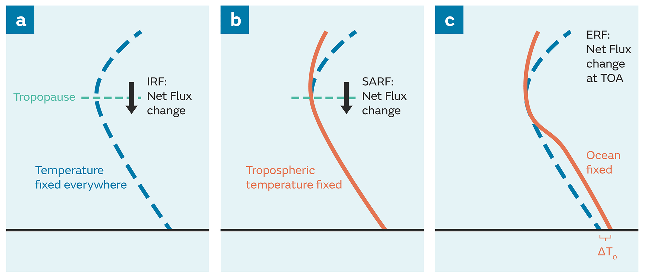
Figure 1 Vertical profiles of temperature showing the different definitions of radiative forcing: (a) instantaneous radiative forcing (IRF), (b) stratospherically adjusted radiative forcing (SARF), and (c) effective radiative forcing (ERF). IRF and SARF are defined at the tropopause whereas ERF is defined at the top of atmosphere (TOA). Adapted from Fig. 8.1 of the IPCC AR5 (Myhre et al., 2013a), which in turn was updated from Hansen et al. (2005).

The aim of the current study is to quantify PD (year 2014) ERFs from anthropogenic drivers of climate change with an atmosphere-only configuration of an ESM. Using the experimental protocol recommended for the Radiative Forcing Model Intercomparison Project (RFMIP; Pincus et al., 2016), PD ERFs will be quantified relative to the PI period from PD–PI changes in emissions, concentrations, and/or land use due to anthropogenic activities. This approach offers a consistent methodology for diagnosing the ERFs of all forcing agents or Earth system (ES) perturbations and, if applied consistently across all models as part of CMIP6 (Eyring et al., 2016), should help to address some of the deficiencies and uncertainties associated with previous estimates of forcing (e.g. Myhre et al., 2013a) and improve our understanding of how the ES responds to forcing (Pincus et al., 2016). The paper is organized as follows. Section 2 provides a brief description of the UK's ESM, UKESM1, used in this study. Section 3 outlines the experimental setup and the simulations carried out. Anthropogenic ERFs are presented in Sect. 4, while conclusions can be found in Sect. 5.

2 Model description

The model used in this study consists of the atmospheric and land components of UKESM1 (Sellar et al., 2019). UKESM1 is based on the Global Atmosphere 7.1/Global Land 7.0 (GA7.1/GL7.0; Walters et al., 2019) configuration of the Hadley Centre Global Environment Model version 3 (HadGEM3; Hewitt et al., 2011), herein referred to as HadGEM3-GA7.1, to which terrestrial carbon/nitrogen cycles (Sellar et al., 2019) and interactive stratosphere–troposphere chemistry (Archibald et al., 2020) from the UK Chemistry and Aerosol (UKCA; Morgenstern et al., 2009; O'Connor et al., 2014) model have been coupled. The model resolution is N96L85; this is equivalent to a horizontal resolution of roughly 135 km and the 85 terrain-following model levels cover an altitude range up to 85 km above sea level. The physical atmosphere model, HadGEM3-GA7.1, already includes the UKCA prognostic aerosol scheme called GLOMAP-mode (Mann et al., 2010; Mulcahy et al., 2018), in which secondary aerosol formation makes use of prescribed oxidant fields. Here, the UKCA chemistry and aerosol schemes are coupled, with oxidants from the stratosphere–troposphere chemistry scheme (Archibald et al., 2020) influencing secondary aerosol formation rates. A full description and evaluation of the UKCA chemistry and aerosol schemes in UKESM1 can be found in Archibald et al. (2020) and Mulcahy et al. (2020), respectively. Mulcahy et al. (2018) also implemented a number of aerosol process improvements in HadGEM3-GA7.1, which helped reduce the aerosol ERF at the present day (year 2000) from −2.75 ± 0.06 W m⁻² in its predecessor model (i.e. HadGEM3-GA7.0; Walters et al., 2019) to −1.45 ± 0.04 W m⁻²; the aerosol ERF in HadGEM3-GA7.0 previously led to an unrealistic negative total anthropogenic ERF of −0.60 W m⁻².

Differences between HadGEM3-GA7.1 and the atmosphere-only configuration of UKESM1 can be found in Table A1 in the Appendix.

3 Model setup and experiments

To calculate the PD (year 2014) ERFs relative to the PI (year 1850) period due to a PD–PI perturbation (e.g. change in emissions), time slice experiments with fixed SSTs and SI were carried out, following the protocol defined by RFMIP (Pincus et al., 2016). The experimental setup was also consistent with recommendations from Forster et al. (2016) and the protocol for time slice ERF experiments defined in AerChemMIP (Collins et al., 2017).

Effectively, this involves running a PI time slice experiment, called piClim-control here, in which SSTs, SI and all other boundary conditions were fixed at year-1850 levels. The SSTs and SI used in piClim-control were monthly mean climatologies derived from 30 years (i.e. years 2156–2185 inclusive) of output from the UKESM1 PI coupled control experiment (piControl) characterized in Sellar et al. (2019) and one of an underpinning set of coupled experiments for CMIP6 (Eyring et al., 2016). It also used 30-year monthly mean climatologies for the vegetation distribution, canopy height, leaf area index (LAI), and surface seawater dimethyl sulfide (DMS) and chlorophyll concentrations derived from the same period of piControl. Fixing the vegetation distribution was not part of the RFMIP protocol and any potential vegetation RAs will be somewhat constrained. This is due to the simulations being based on the configuration of UKESM1 used for the Atmosphere Model Intercomparison Project (AMIP) simulation (which prescribed vegetation characteristics). Although the AerChemMIP protocol (Collins et al., 2017) requested use of the maximum capability possible, interactive vegetation was not a model requirement. The extra RFMIP experiments carried out here were only done as a late addition and the same experimental setup was kept for internal consistency.

The model was initialized using output from the start of the 30-year period used to produce the PI climatologies (i.e. January 2156 of piControl). All the other experiments are perturbation experiments, parallel to piClim-control, in which selected emissions, concentrations, and/or land use were changed from year-1850 to year-2014 values. Although AerChemMIP and RFMIP recommend 30 years for fixed SST (fSST) time slice ERF experiments, the perturbations to the LLGHGs took up to 15 years to propagate fully into the stratosphere due to the turnover timescale associated with the Brewer–Dobson circulation (e.g. Butchart, 2014). Therefore, all simulations were 45 years in length. Using the latter 30 years of the paired simulations, the ERFs were diagnosed as the time-mean global-mean PD–PI difference in the TOA net radiative fluxes. Running for 30 years when the model has reached steady state reduces the uncertainty associated with meteorological variability (e.g. Shindell et al., 2013a) and improves the estimate of the ERF. Details on how the ERF was further decomposed can be found in Sect. 4.

In all cases, the GHG concentrations for 1850 and/or 2014 were taken from Meinhausen et al. (2017). However, the recommended concentrations for the different GHGs in UKESM1 are implemented differently. In the case of CO₂, the prescribed concentration is uniform in mass mixing ratio throughout the model domain. For methane (CH₄) and nitrous oxide (N₂O), the recommended concentrations are treated as lower boundary conditions (LBCs); their 3D distributions are modelled interactively by the UKCA chemistry scheme (Archibald et al., 2020) and coupled to radiation. For O₃-depleting substances (ODSs) or halocarbons (HCs) in piClim-HC, their concentrations are prescribed separately (and consistently) in UKCA and in the radiation scheme. For the UKCA chemistry scheme, LBCs are prescribed for trichlorofluoromethane (CFC11), dichlorodifluoromethane (CFC12), and methyl bromide (CH₃Br), all of which include contributions from other chlorine- and bromine-containing source gases not explicitly treated in UKCA. This approach ensures that the correct stratospheric chlorine and bromine loadings are used for the PD period. Further details on the species included in the CFC11, CFC12, and CH₃Br LBCs can be found in Archibald et al. (2020). For the radiation scheme, the radiative effects of ODSs are handled by prescribing the mass mixing ratio of a lumped species (CFC12-eq) uniformly throughout the atmosphere, consistent with the UKCA LBCs. Finally, the piClim-GHG experiment collectively perturbs all the GHGs from PI to PD levels, including non-O₃-depleting HCs. For these latter GHGs, a uniform mass mixing ratio of a lumped species (HFC134a-eq), provided by Meinhausen et al. (2017), is prescribed in the radiation scheme.

Table 1 List of all the atmosphere-only experiments carried out with the UK's Earth System Model, UKESM1, to quantify PD ERFs from PD–PI changes in emissions, concentrations, and/or land use. Each simulation was 45 years in length, with analysis based on the last 30 years.

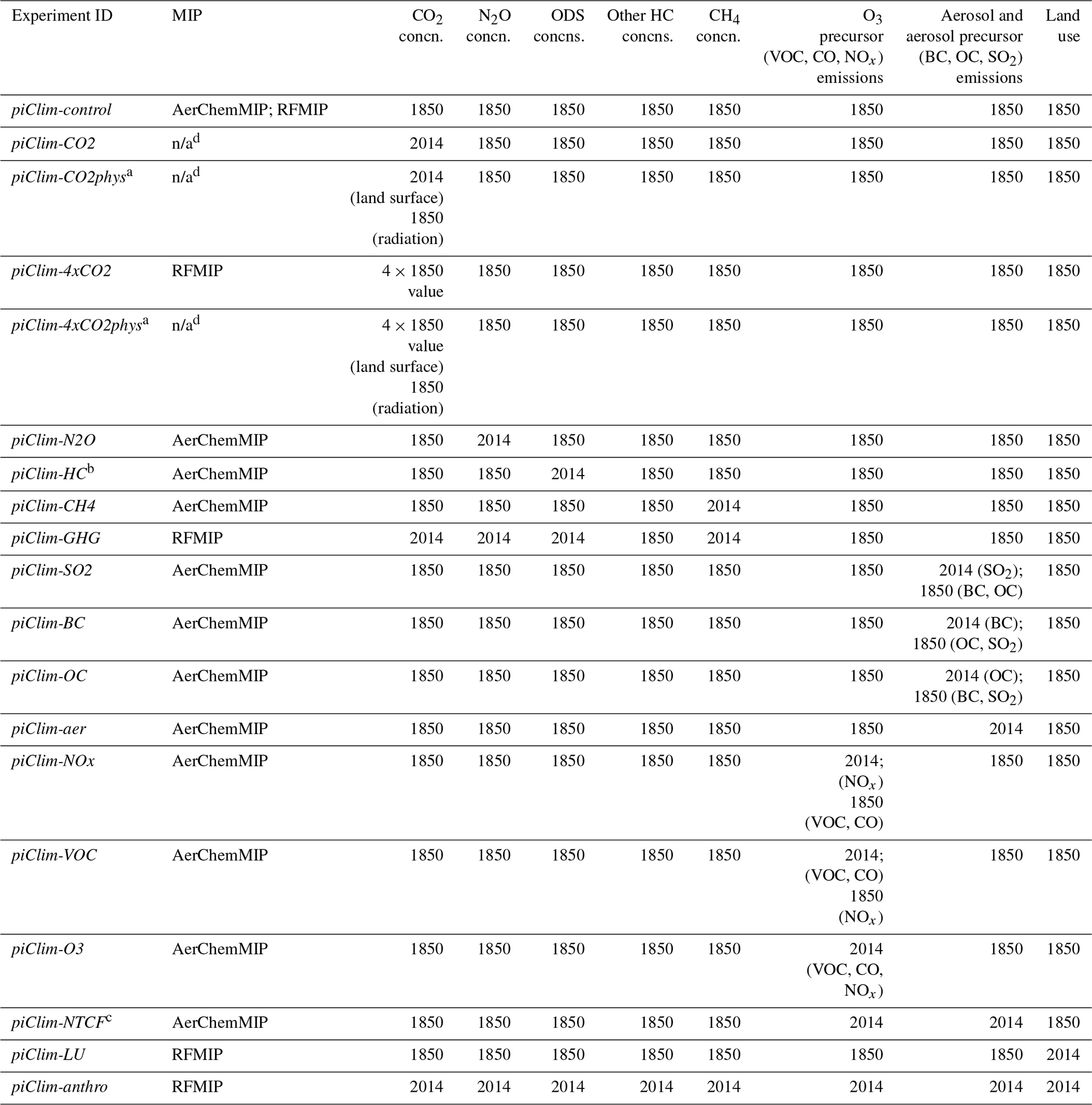
^a In the piClim-CO2phys and piClim-4xCO2phys simulations, only the land surface sees the perturbation in CO₂; the radiation scheme still sees the PI concentration. ^b The AerChemMIP experiment piClim-HC changes concentrations of ODSs or O₃-depleting halocarbons (HCs) from PI to PD levels. ^c The AerChemMIP experiment piClim-NTCF is also known as piClim-aerO3 in RFMIP. ^d n/a: not applicable.

In all the experiments in Table 1, anthropogenic and biomass burning emissions of primary aerosol and aerosol precursors (BC, organic carbon (OC), and sulfur dioxide (SO₂)) and O₃ precursors (volatile organic compounds (VOCs), carbon monoxide (CO), and nitrogen oxides (NO_x)) excluding CH₄ for 1850 and/or 2014 were taken from Hoesly et al. (2018) and van Marle et al. (2017). In the case of the NO_x emissions perturbation experiment (piClim-NOx), both aircraft and surface anthropogenic and biomass burning emissions were changed to PD levels. In piClim-VOC, both VOC and CO anthropogenic and biomass burning emissions were changed to PD levels, while the experiment piClim-O3 perturbs emissions of VOC, CO, and NO_x only, with the CH₄ concentration remaining at PI levels. Finally, although near-term climate forcers (NTCFs) include CH₄ and short-lived HCs (e.g. Myhre et al., 2013a), in the context of the AerChemMIP protocol (Collins et al., 2017), the experiment piClim-NTCF does not perturb concentrations of CH₄ or other short-lived GHGs. It only changes anthropogenic and biomass burning emissions of aerosol and aerosol precursors (BC, OC, and SO₂) and O₃ precursors (VOC, CO, NO_x) to PD levels; it is also referred to as piClim-aerO3 in the RFMIP protocol (Table 1).

For prescribing the anthropogenic LU change at 2014, the difference in vegetation between 1850 and 2014 was taken from a UKESM1 coupled historical simulation, in which the only transient forcing was anthropogenic LU change. Natural volcanic and solar forcings were fixed in all simulations at 1850 levels (Arfeuille et al., 2014; Thomason et al., 2018; Matthes et al., 2017) using those specified for CMIP6 (Eyring et al., 2016). Table 1 gives a full list of the fSST ERF experiments carried out with UKESM1 for this study. The only experiment omitted from the fSST ERF experiments specified in the RFMIP and AerChemMIP protocols is piClim-NH3; this is because UKESM1's aerosol scheme, GLOMAP-mode (Mann et al., 2010; Mulcahy et al., 2018, 2020), does not include any treatment for nitrate aerosol.

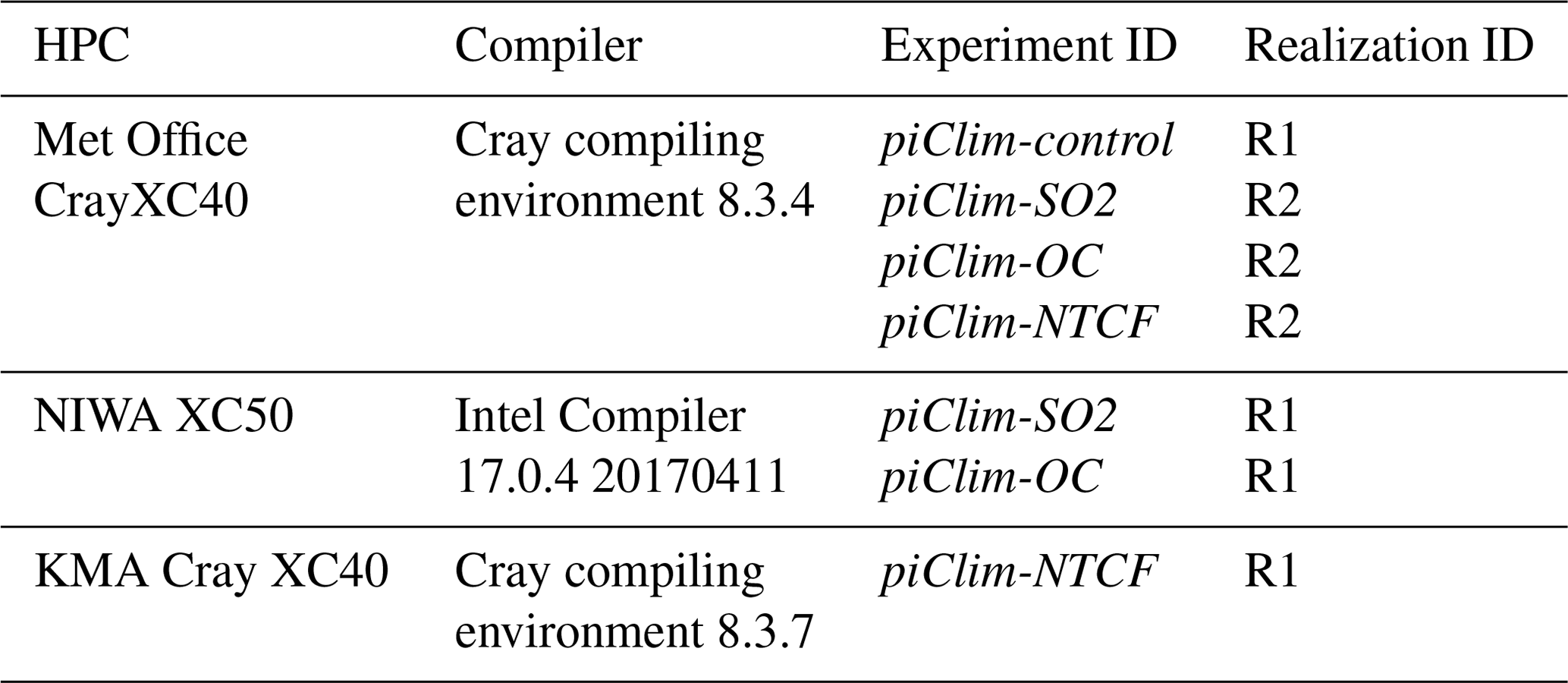
Through a partnership between the Met Office Hadley Centre (MOHC; https://www.metoffice.gov.uk/climate-guide/science/science-behind-climate-change/hadley, last access: 15 January 2021), the UK's National Centre for Atmospheric Science (NCAS; https://www.ncas.ac.uk/en/, last access: 15 January 2021), New Zealand's National Institute for Water and Atmospheric Research (NIWA; https://www.niwa.co.nz/, last access: 15 January 2021), and the National Institute of Meteorological Science/Korean Meteorological Administration (NIMS-KMA; http://www.nimr.go.kr/AE/?sub_num=130, last access: 15 January 2021), the fSST experiments carried out with UKESM1 were spread across multiple high-performance computing (HPC) platforms. Due to the non-linearity of the equations being solved, ESMs are sensitive to the propagation of small perturbations, resulting in a lack of bit reproducibility. As a result, we aimed to verify that the differences in model output were not statistically significant from each other.

To test this, we created an ensemble of short runs on each machine by perturbing selected variables in their initial conditions, using a perturbation with a numerical value comparable to the machine's precision. The spread of results (at each point in time and space) on each platform was then used to determine whether they could each have been sampled from the same ensemble of results generated on either machine. A permutation method was used to ensure statistical independence between neighbouring points according to the work described by Wilks (1997). A paper describing this protocol in more detail is in preparation (Teixeira, 2020). In addition to this, a number of perturbation experiments were carried out in duplicate to test the sensitivity of the ERFs to differences in the HPC platforms. These duplicate experiments are listed in Table 2 and will be available through the Earth System Grid Federation (ESGF; https://esgf.llnl.gov/, last access: 15 January 2021) archive as different realizations of the same experiment.

Table 2 List of atmosphere-only PI control (piClim-control) and duplicate perturbation experiments (piClim-X) carried out with UKESM1 on different HPC platforms.

4 Anthropogenic effective radiative forcings (ERFs)

The ERF has been calculated from the difference (Δ) in the net TOA radiative flux (F) between the perturbed simulation (e.g. piClim-CH4; Table 1) and the piClim-control simulation as follows:

$$\begin{array}{}\text{(3)}& \mathrm{ERF}=\mathrm{\Delta }F,\end{array}$$

where ΔF is in response to whole-atmosphere PD–PI changes in composition and/or other RAs; no masking of the response is applied. For example, the ERF quantified from piClim-HC minus piClim-control includes the direct radiative effect from the increase in ODS concentrations, the indirect radiative effect of the whole-atmosphere O₃ response, as well as other changes to the TOA radiative fluxes due to whole-atmosphere and land surface RAs. The ERF can be decomposed into the clear-sky (CS) ERF (ERF_cs) and the change in the cloud radiative effect (ΔCRE) using the diagnosed CS radiative flux (F_cs):

$$\begin{array}{}\text{(4)}& {\displaystyle }\mathrm{ERF}=\mathrm{\Delta }{F}_{\mathrm{cs}}+\mathrm{\Delta }\left(F-F_{\mathrm{cs}}\right)\text{(5)}& {\displaystyle }={\mathrm{ERF}}_{\mathrm{cs}}+\mathrm{\Delta }\mathrm{CRE}.\end{array}$$

However, many of the experiments in this study either directly perturb aerosol emissions and/or alter aerosol concentrations via chemical and dynamical interactions. Changes in aerosol can bias the diagnosed CRE as aerosol scattering and absorption typically reduce the contrast in SW reflection between cloudy and CS scenes; this process is termed “cloud masking” (e.g. Zelinka et al., 2014). In consideration of this, we have calculated the change in the CRE from “clean” radiation calls that exclude ARI, as recommended in Ghan (2013):

$$\begin{array}{}\text{(6)}& {\displaystyle }\begin{array}{rl}\mathrm{ERF}=& \mathrm{\Delta }\left(F-F_{\mathrm{clean}}\right)+\mathrm{\Delta }{F}_{\mathrm{cs},\mathrm{clean}}\\ & +\mathrm{\Delta }\left(F_{\mathrm{clean}}-F_{\mathrm{cs},\mathrm{clean}}\right)\end{array}\text{(7)}& {\displaystyle }=\mathrm{Aerosol}\mathrm{IRF}+{\mathrm{ERF}}_{\mathrm{cs},\mathrm{clean}}+\mathrm{\Delta }{\mathrm{CRE}}^{\prime }\text{(8)}& {\displaystyle }={\mathrm{ERF}}_{\mathrm{cs}}^{\prime }+\mathrm{\Delta }{\mathrm{CRE}}^{\prime }.\end{array}$$

The ERF is, thus, separated into a component due to cloud property changes (ΔCRE^′) and the non-cloud forcing (${{\mathrm{ERF}}_{\mathrm{cs}}}^{\prime }$). Here, ${{\mathrm{ERF}}_{\mathrm{cs}}}^{\prime }$ is the sum of the aerosol IRF and any non-aerosol-driven changes in CS fluxes and differs slightly from ERF_cs in Eq. (5), in that it can include the impact of aerosol scattering and absorption in the clear-air above or below clouds. One acknowledged limitation is that variations in gaseous absorption and emission between clear and cloudy scenes also lead to cloud masking effects (e.g. Soden et al., 2008). Although Ghan's method removes the very prominent influence of aerosols, cloud masking from O₃ and other GHGs may still affect the separation of ERF into its CS and CRE components.

4.1 Overview of ERFs

The ERF, and its CS (${{\mathrm{ERF}}_{\mathrm{cs}}}^{\prime }$) and ΔCRE^′ contributions, following Eq. (8), are listed in Table 3 for all perturbation experiments relative to piClim-control and are further decomposed into the SW (solar), LW (terrestrial), and net (SW + LW) components. Table 3 also includes estimates of the model-derived uncertainty in the different components by calculating the standard error based on Forster et al. (2016). Although the errors quoted are small (i.e. less than 0.04 W m⁻²), they do not represent the true uncertainty in the quantified ERFs; uncertainties due to emissions (e.g. Hoesly et al., 2018), model biases (e.g. Archibald et al., 2020), incorrect sensitivity to changing emissions (e.g. Archibald et al., 2010; Wild et al., 2020), radiative transfer schemes (e.g. Pincus et al., 2020), and/or missing or unresolved processes are not taken into account.

Table 3 Present-day (year 2014) ERFs relative to the pre-industrial (year 1850) period derived from Eq. (8) and including an estimate of the standard error. Where duplicate experiments exist (e.g. piClim-SO2; Table 2), the quoted ERFs are based on Realization IDs R2. Units in W m⁻².

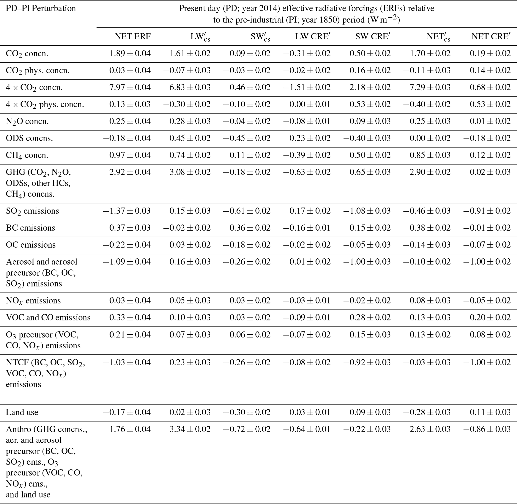
The ERFs are also plotted in Fig. 2. Together, they show that the ERF from GHGs is 2.92 ± 0.04 W m⁻², which is offset by an aerosol ERF of −1.09 ± 0.04 W m⁻². The GHG ERF estimate is lower and the aerosol ERF is consistent with estimates of 3.09 and −1.10 W m⁻², respectively (Andrews et al., 2019), from the HadGEM3 GC3.1 (Williams et al., 2017) physical model (herein referred to as HadGEM3-GC3.1) upon which UKESM1 is based but are consistent with the range of previous estimates (e.g. Myhre et al., 2013a). The net anthropogenic ERF is 1.76 ± 0.04 W m⁻², again consistent with the range of estimates from AR5 (Myhre et al., 2013a) and the estimate from HadGEM3-GC3.1 (1.81 W m⁻²; Andrews et al., 2019). The net anthropogenic ERF quantified here is also narrowly inside the range of net anthropogenic ERF of 2.3 W m⁻² (1.7 to 3.0 W m⁻²; 5 %–95 % confidence interval) derived from a top-down energy budget constraint based on measurements of historical global mean temperature change, the Earth's heat uptake, and model estimates of the Earth's radiative response (Andrews and Forster, 2020).

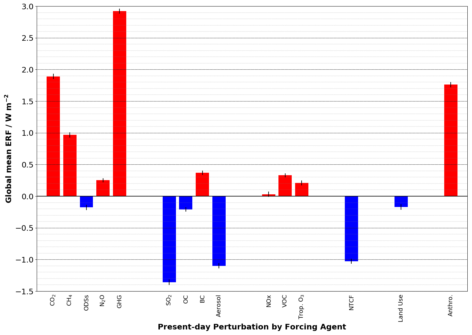
Figure 2 Present day (year 2014) anthropogenic ERFs relative to the pre-industrial (year 1850) period derived from Eq. (8), and including an estimate of the standard error. Units in W m⁻².

Figure 3 shows global and zonal mean distributions of the ERFs from PD–PI changes in GHG concentrations, aerosol and aerosol precursor (BC, OC. SO₂) emissions, O₃ precursor (VOC, CO, NO_x) emissions, LU change, and total anthropogenic sources. It shows that the ERF from GHGs (Fig. 3a) has a robust signal over 93 % of the globe; it is positive everywhere except for the southern high latitudes (Fig. 3b). This negative ERF is due to the negative ERF from the piClim-HC perturbation experiment (Table 3) which offsets the positive ERFs from the other LLGHG experiments. The breakdown of the GHG ERF into its individual speciated contributions will be discussed further in Sect. 4.2 and results from piClim-HC will be discussed in Sect. 4.2.3. The aerosol ERF (Fig. 3c and d) is robust over a smaller area (52 %) of the globe and is more spatially heterogeneous than the GHG ERF due to the shorter aerosol lifetime. However, the distribution of the aerosol ERF is mostly negative, except for over bright surfaces and regions where the positive forcing from BC emissions outweighs the negative forcing from scattering aerosols such as sulfate and OC. A breakdown of the aerosol ERF between constituents and between ARI and ACI will be presented and discussed in Sect. 4.3.

Figure 3e and f show the global and zonal mean distributions of the ERF from emissions of O₃ precursors (VOC, CO, and NO_x), excluding CH₄. It shows that the ERF from changes in VOC, CO, and NO_x emissions alone is positive (0.21 ± 0.04 W m⁻²; Table 3), but with only 10 % of the globe showing a robust signal. Further analysis of the ERF from O₃ precursor emissions and their contribution, along with CH₄, to tropospheric O₃ RF, can be found in Sect. 4.4.2. The distribution of a robust LU ERF (Fig. 3g, h) is also limited in spatial extent (∼ 12 % of the globe); much of the negative ERF is concentrated over the Northern Hemisphere (NH) continental regions (e.g. North America, South East Asia). Together with aerosols, the combined ERF outweighs the positive ERF from GHGs, leading to a negative total anthropogenic ERF over parts of the NH continents (Fig. 3i). As was the case with the GHG ERF, the negative ERF over the Southern Hemisphere (SH) high latitudes is still evident in the total anthropogenic ERF (Fig. 3i, j).

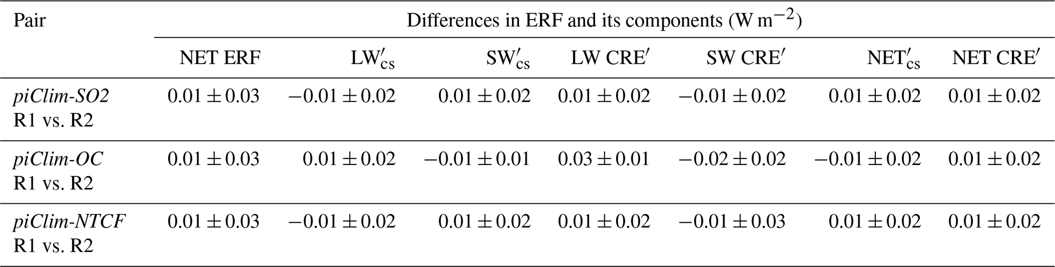
As discussed in Sect. 3, the UKESM1 fSST experiments were run on multiple HPC platforms. Statistical methods ensure that the model is not scientifically different on the different HPC platforms, but such duplicate experiments still produce slightly different results. This raises the question of the impact of such differences on the quantification of ERFs with UKESM1. To address this question, the experiments described in Table 2 were used to compare the difference in TOA radiative fluxes of equivalent realization experiment pairs. The two-sample Kolmogorov–Smirnov test between the monthly TOA radiative fluxes from the realization pairs (null hypothesis that the samples are drawn from the same distribution) shows that the TOA radiative fluxes between the two realization pairs are statistically identical at a confidence level (α) of 5 % (Table 4). Despite the fact that one cannot conclude that the distributions are identical, for each pair of experiments there is no evidence suggesting that the two distributions are different.

Table 4 Differences in the present-day ERF and its components between two realizations (R1 and R2) of the same perturbation experiment relative to piClim-control. Units in W m⁻².

4.2 Long-lived greenhouse gases (LLGHGs)

4.2.1 Carbon dioxide (CO₂)

Atmospheric CO₂ concentrations have risen from 284.3 to 397.5 ppm between 1850 and 2014 (Meinshausen et al., 2017) resulting in an ERF of 1.89 ± 0.04 W m⁻² (Table 3) and is the largest individual contribution to the total historical forcing. Myhre et al. (2013a) report a SARF of 1.82 ± 0.19 W m⁻² for the period from 1750 to 2011, which, coincidentally, has a near identical rise in CO₂ of 113 ppm to that assessed here, although CO₂ forcing has a logarithmic dependency on concentration. An updated assessment based on line-by-line calculations (Etminan et al., 2016) increased SARF for 2015 relative to 1750 to 1.95 W m⁻² but for a larger CO₂ rise of 121 ppm. Applying the CO₂ SARF formula from Etiminan et al. (2016) to our case reveals a SARF of 1.80 W m⁻². Our ERF estimate for 2014 is, therefore, larger than the SARF by 0.09 W m⁻². As expected for a GHG, the ERF is dominated by the LW${}_{\mathrm{cs}}^{\prime }$ component (1.61 ± 0.02 W m⁻²) with an additional contribution from the SW${}_{\mathrm{cs}}^{\prime }$ component (0.09 ± 0.02 W m⁻²) coming from direct effects and an RA in snow cover across the northern latitudes. There is also a NET CRE^′ contribution (0.19 ± 0.02 W m⁻²) from a reduction in cloud cover. The SW direct effect occurs in the near-infrared and is small, equivalent to around 2 % of the LW forcing (Pincus et al., 2020). On that assumption, the SW${}_{\mathrm{cs}}^{\prime }$ component is dominated by the rapid albedo adjustment over the direct effect.

Rising atmospheric CO₂ also exerts an indirect forcing through rapid changes in plant stomatal conductance (Doutriaux-Boucher et al., 2009; Richardson et al., 2018) enhancing plant water use efficiency and reducing evapotranspiration leading to an increase in sensible heating at the surface and corresponding drying of the boundary layer and reduction in low clouds. This mechanism is known as a physiological forcing. In UKESM1 (piClim-CO2phys; Table 3), this forcing is small at PD and 4× CO₂ levels (0.03 ± 0.04 and 0.13 ± 0.03 W m⁻²), and scales in line with the total CO₂ ERF. It results from a balance between a negative LW${}_{\mathrm{cs}}^{\prime }$ component (−0.07 ± 0.03; −0.30 ± 0.02 W m⁻²) associated with surface warming and a positive SW CRE^′ component (0.16 ± 0.02; 0.53 ± 0.02 W m⁻²) associated with a reduction in low-level clouds and from smaller terms including a negative SW${}_{\mathrm{cs}}^{\prime }$ component from reduced water vapour. Previous Hadley Centre models at 4 × CO₂ found a similar but larger effect: 1.1 W m⁻² in HadCM3LC (Doutriaux-Boucher et al., 2009) and 0.25 W m⁻² in HadGEM2-ES (Andrews et al., 2012b). We find that UKESM1 has a similar LW${}_{\mathrm{cs}}^{\prime }$ component compared to HadGEM2-ES implying that UKESM1 has a similar surface warming adjustment associated with the physiological effect but offset by a weaker SW CRE^′ component. The inclusion of the physiological effect and rapid albedo adjustment in the CO₂ ERF acts to increase the forcing slightly. These additional adjustments likely account for our slightly higher ERF relative to the SARF from line-by-line estimates (Etminan et al., 2016).

4.2.2 Nitrous oxide (N₂O)

The ERF due to changes in N₂O concentration from the PI period (273 ppbv in 1850) to the present day (327 ppbv in 2014) is calculated as 0.25 ± 0.04 W m⁻² (Table 3), following Eq. (8) described above. The predominant contribution to the N₂O ERF is the LW${}_{\mathrm{cs}}^{\prime }$ component (0.28 ± 0.03 W m⁻²), with a small offset by the SW${}_{\mathrm{cs}}^{\prime }$ component (−0.04 ± 0.02 W m⁻²); the NET${}_{\mathrm{cs}}^{\prime }$ component sums up to 0.25 ± 0.03 W m⁻². The NET CRE^′ component is insignificant (0.01 ± 0.03 W m⁻²), with SW CRE^′ and LW CRE^′ contributions of 0.09 ± 0.03 W m⁻² and −0.08 ± 0.02 W m⁻², respectively. In comparison, the net ERF calculated here (0.25 ± 0.04 W m⁻²) is higher than the SARF values of 0.17 ± 0.03 W m⁻² from AR5 for 2011 (Myhre et al., 2013a) and of 0.18 W m⁻² for 2014 based on the updated expression from Etminan et al. (2016). This is likely to be due to the effect of adjustments associated with changing N₂O that were not considered as part of the SARF in AR5 (Myhre et al., 2013a) or Etminan et al. (2016), including O₃ depletion and fast cloud adjustments. The UKESM1 estimate agrees well with the AerChemMIP multi-model mean of 0.23 ± 0.05 W m⁻² (Thornhill et al., 2020). Previously, Hansen et al. (2005) calculated an IRF and a SARF of 0.15 W m⁻² due to the change in N₂O from 278 to 316 ppbv.

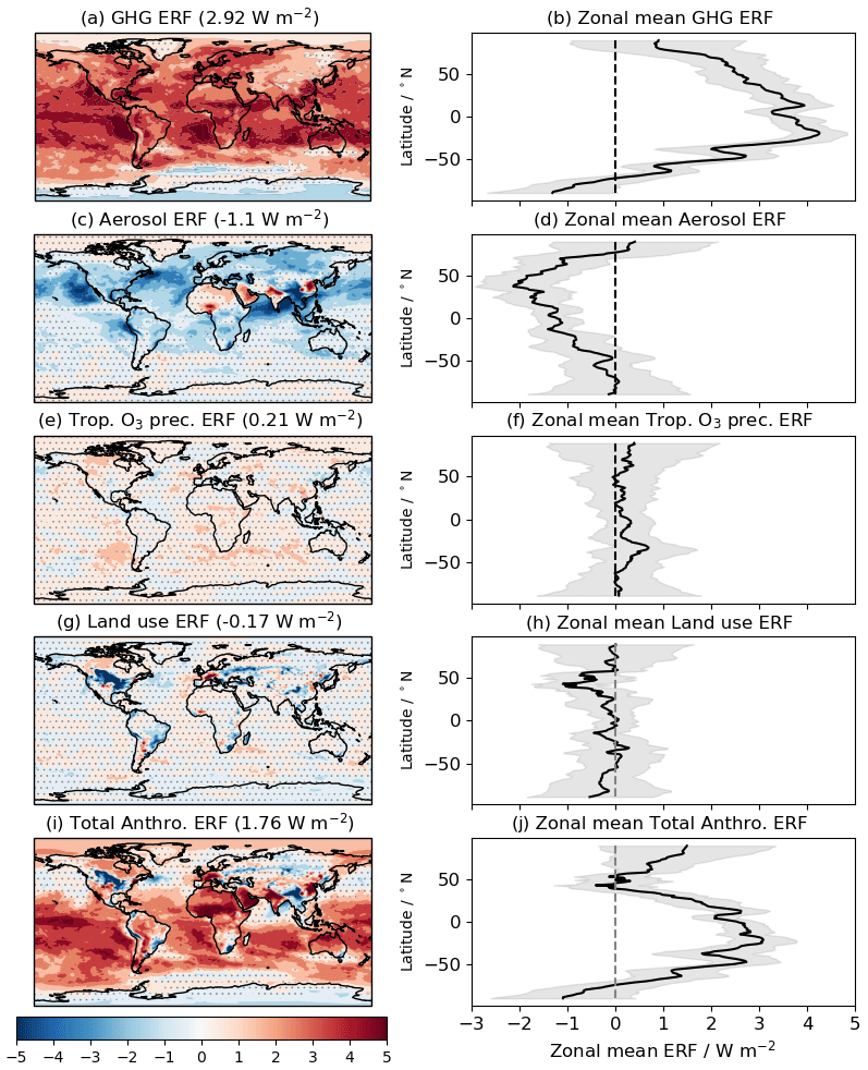
Figure 3 Geographical and zonal mean distributions of the present-day (PD; year 2014) ERFs relative to the pre-industrial (PI; year 1850) period in (a) and (b) for GHGs, in (c) and (d) for aerosols, in (e) and (f) for O₃ precursors, in (g) and (h) for LU change, and in (i) and (j) for total anthropogenic, respectively. In the global distribution plots, global mean ERFs are included and areas are stippled where the ERF is not statistically significant at the 95 % confidence interval. In the zonal mean plots, the grey shading shows the ± 1 standard deviation in the zonal mean ERF. Units in W m⁻².

The global distribution of the individual components contributing to the N₂O ERF (Fig. 4) shows that the SW${}_{\mathrm{cs}}^{\prime }$ component is negligible. The LW${}_{\mathrm{cs}}^{\prime }$ component is predominantly positive, due mainly to N₂O direct forcing. The SW CRE^′ and LW CRE^′ components of the ERF are largely noise (at 95 % confidence level; Fig. 4), with a net contribution to the ERF of close to zero.

Figure 4 Global distributions of the PD N₂O ERF components relative to the PI period, i.e. piClim-N2O minus piClim-control; (a) SW${}_{\mathrm{cs}}^{\prime }$, (b) SW CRE^′, (c) LW${}_{\mathrm{cs}}^{\prime }$, (d) LW CRE^′, (e) NET${}_{\mathrm{cs}}^{\prime }$, and (f) NET CRE^′, based on Eq. (8). Global mean values are shown in brackets. Regions where the ERF components are outside the 95 % confidence level are stippled. Units in W m⁻².

4.2.3 Ozone (O₃)-depleting substances (ODSs)

The ERF from the PD–PI change in ODSs is quantified, using piClim-HC relative to piClim-control, as −0.18 ± 0.04 W m⁻², which is dominated by the NET CRE^′ component (−0.18 ± 0.02 W m⁻²; Table 3). Figure 5 shows global distributions of the SW${}_{\mathrm{cs}}^{\prime }$, SW CRE^′, LW${}_{\mathrm{cs}}^{\prime }$, LW CRE^′, NET${}_{\mathrm{cs}}^{\prime }$, and NET CRE^′ components, respectively. For CS conditions, the SW component (SW${}_{\mathrm{cs}}^{\prime }$) is characterized by negative values over the southern high latitudes (to a lesser extent in the northern high latitudes), which is linked to pronounced Antarctic O₃ depletion and some decreases in Arctic O₃ (not shown). The LW${}_{\mathrm{cs}}^{\prime }$ component is predominantly positive, reflecting the direct effect of ODSs acting as GHGs in the piClim-HC simulation. The positive LW${}_{\mathrm{cs}}^{\prime }$ component at high latitudes contains an offset caused by O₃ depletion. Overall, the global mean NET${}_{\mathrm{cs}}^{\prime }$ component is negligible (0.00 ± 0.02 W m⁻²; Table 3). Under cloudy conditions, the negative SW CRE^′ component and the positive LW CRE^′ component of the ERFs are anti-correlated, especially over the Southern Ocean, summing up to a net contribution to the ERF of −0.18 ± 0.02 W m⁻².

As mentioned previously, the ERF includes the direct effect of the ODSs acting as GHGs, the indirect effect of the O₃ depletion that they cause, and any resulting TOA changes due to other RAs. Quantifying the historical evolution of the total O₃ RF alone from the CMIP6 models, Skeie et al. (2020) found that UKESM1 was the only model with both tropospheric and stratospheric chemistry that had a negative total O₃ RF at the present day. This is likely due to UKESM1 having a global O₃ decline during the period of increasing ODSs that is stronger than other models and observations by at least a factor of 1.4 (Table 2 in Keeble et al., 2020). Likewise, in the AerChemMIP multi-model ODS ERF assessment, Morgenstern et al. (2020) used observed O₃ trends as a constraint on the modelled ODS ERF; they found that the ERF is likely to be between −0.05 and 0.13 W m⁻², with the UKESM1 estimate of −0.18 ± 0.04 W m⁻² outside of this range. Although Keeble et al. (2020), Skeie et al. (2020) and Morgenstern et al. (2020) suggest that the negative contribution from O₃ depletion to the ODS ERF is too strong in UKESM1, there is an additional negative offset to the direct radiative effect of the ODSs through the NET CRE^′ component (Fig. 5). Furthermore, the ODSs will have an impact on tropospheric O₃; their contribution to the tropospheric O₃ RF will be quantified in Sect. 4.4.2.

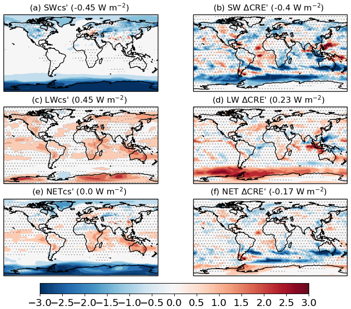
Figure 5 Global distributions of the PD ODS ERF components relative to the PI period, i.e. piClim-HC minus piClim-control; (a) SW${}_{\mathrm{cs}}^{\prime }$, (b) SW CRE^′, (c) LW${}_{\mathrm{cs}}^{\prime }$, (d) LW CRE^′, (e) NET${}_{\mathrm{cs}}^{\prime }$, and (f) NET CRE^′, based on Eq. (8). Global mean values are shown in brackets. Regions where the ERF components are outside the 95 % confidence level are stippled. Units in W m⁻².

4.2.4 Methane (CH₄)

The global mean CH₄ concentration changed from 808.3 ppbv in the PI (year 1850) period to 1831.5 ppbv in the PD (year 2014) period, resulting in an ERF of 0.97 ± 0.04 W m⁻² (Table 3; Fig. 6). Most of the ERF (0.74 ± 0.02 W m⁻²; Table 3) is due to the LW${}_{\mathrm{cs}}^{\prime }$ component, with an additional positive contribution (0.11 ± 0.02 W m⁻²) from the SW${}_{\mathrm{cs}}^{\prime }$ component, which is consistent with the growing recognition of the importance of the SW absorption bands in CH₄ forcing (Collins et al., 2006; Li et al., 2010; Etminan et al., 2016). There are additional SW and LW CRE^′ components but these partly cancel out, leading to a small NET CRE^′ (0.12 ± 0.02 W m⁻²) in addition to the NET${}_{\mathrm{cs}}^{\prime }$ component (0.85 ± 0.03 W m⁻²). Estimates of the direct CH₄ ERF from HadGEM2 model simulations (Andrews, 2014) and the updated RF expression for CH₄ based on line-by-line calculations (Etminan et al., 2016) are on the order of 0.50–0.56 W m⁻², but the ERF calculated here is higher by more than 0.4 W m⁻². However, it is consistent with other studies (e.g. Hansen et al., 2005; Shindell et al., 2009; Myhre et al., 2013a), which concluded that the total climate forcing by CH₄ is almost double that of the direct forcing and is due to indirect effects. The UKESM1 estimate is also larger than the 0.69 W m⁻² radiative impact of an increase in CH₄ concentration of 1800 ppbv above PD levels quantified by Winterstein et al. (2019) with the ECHAM/MESSy Atmospheric Chemistry (EMAC) coupled model. Although the Winterstein et al. (2019) estimate included indirect forcings from O₃ and stratospheric water vapour (SWV), their direct CH₄ forcing in the LW is low relative to other models (Lohmann et al., 2010).

Figure 6 Global distributions of the PD CH₄ ERF components relative to the PI period, i.e. piClim-CH4 minus piClim-control; (a) SW${}_{\mathrm{cs}}^{\prime }$, (b) SW CRE^′, (c) LW${}_{\mathrm{cs}}^{\prime }$, (d) LW CRE^′, (e) NET${}_{\mathrm{cs}}^{\prime }$, and (f) NET CRE^′, based on Eq. (8). Global mean values are shown in brackets. Regions where the ERF components are outside the 95 % confidence level are stippled. Units in W m⁻².

The UKESM1 ERF quantified here is at the upper end of estimates from the recent study of AerChemMIP multi-model ERFs by Thornhill et al. (2020). They found that the multi-model mean ERF was 0.70 W m⁻², with a standard deviation of 0.22 W m⁻². They attributed part of the inter-model spread to different complexities in the representation of interactive chemistry in the respective models, i.e. some models only captured the direct radiative effect of CH₄ (e.g. NorESM2) while others (e.g. UKESM1) also included indirect contributions from CH₄-driven changes in O₃ and SWV. However, the contribution to the ERF from tropospheric adjustments differed in both magnitude and sign between the models, with UKESM1 being the only model with a positive contribution to the ERF from tropospheric RAs. The relative contributions of the direct and indirect contributions to the total CH₄ ERF quantified here and the mechanism behind the positive tropospheric RA can be found in O'Connor et al. (2019).

4.2.5 Total greenhouse gases (GHGs)

The major drivers of anthropogenic climate change are GHGs, whose forcing is offset by aerosols (Myhre et al., 2013a). Therefore, the total GHG ERF and the aerosol ERF are key values in understanding observed and modelled changes in the climate system since the PI period. As a result, a separate time slice simulation with all GHG concentrations (piClim-GHG; Table 1) at PD levels was conducted following the RFMIP protocol (Pincus et al., 2016).

The UKESM1 piClim-GHG experiment leads to an ERF of 2.92 ± 0.04 W m⁻² (Table 3), which is dominated by a positive LW${}_{\mathrm{cs}}^{\prime }$ component (3.08 ± 0.02 W m⁻²) that is partially offset by a negative SW${}_{\mathrm{cs}}^{\prime }$ component (−0.18 ± 0.02 W m⁻²). There are significant positive and negative contributions from the SW CRE^′ (0.65 ± 0.03 W m⁻²) and the LW CRE^′ (−0.63 ± 0.02 W m⁻²) components, but these largely cancel out and contribute little (0.02 ± 0.03 W m⁻²) to the total ERF (Table 3). This GHG ERF is lower than the ERF of 3.09 W m⁻² estimated from the physical model HadGEM3-GC3.1 (Andrews et al., 2019). Part of this discrepancy may be due to the inclusion in UKESM1 of indirect forcings by O₃ and/or aerosols from ODSs (Morgenstern et al., 2020) and CH₄ (O'Connor et al., 2020), for example. The UKESM1 estimate, however, is consistent with the AR5 year-2011 SARF estimate of 2.82 W m⁻². The latter estimate of 2.82 W m⁻² has been adjusted to an 1850 baseline from 1750, and taking stratospheric O₃ depletion, CH₄-driven SWV, and half of the tropospheric O₃ forcing (based on the attribution by Stevenson et al., 2013) into account, although some GHG concentrations (e.g. CH₄, CO₂) have increased between 2011 and 2014 (Nisbet et al., 2016) while others (e.g. ODSs) have declined (Engel et al., 2018).

The simulation piClim-GHG perturbs non-O₃-depleting HCs but piClim-HC does not. Nevertheless, the small positive RF from non-O₃-depleting HCs of 0.02 W m⁻² in 2011 (Myhre et al., 2013a) allows one to use the combination of GHG simulations to test for linearity. The sum of the ERFs from piClim-CO2, piClim-CH4, piClim-N2O, and piClim-HC is 2.93 ± 0.08 W m⁻², indicating that the ERFs add linearly and agree with the ERF from piClim-GHG (2.92 ± 0.04 W m⁻²).

4.3 Aerosols and aerosol precursors

Figure 7a summarizes the results from the anthropogenic aerosol experiments, including a breakdown of the ERF into IRF and RAs for each of the anthropogenic aerosol experiments (piClim-SO2, piClim-OC, piClim-BC, and piClim-aer). The IRF was calculated using the double-call system where ARI (i.e. scattering and absorption) are withdrawn from the second call to the radiation scheme, as in Ghan et al. (2012). The RAs have then been derived as the residual between the ERF and IRF and include all aerosol-induced changes in cloud radiative effects. For completeness, Table 3 also summarizes the contributions to the ERF from the SW${}_{\mathrm{cs}}^{\prime }$, SW CRE^′, LW${}_{\mathrm{cs}}^{\prime }$, LW CRE^′, NET${}_{\mathrm{cs}}^{\prime }$, and NET CRE^′ components quantified using Eq. (8).

Uncertainties in aerosol ERF are driven partly by uncertainties in aerosol lifetime, spatial and temporal distributions, the historical change in aerosol loading, and the cloud response to aerosols (Bellouin et al., 2020). Other contributing factors include uncertainties in the PI aerosol state (Carslaw et al., 2013) as well as the oxidizing capacity of the atmosphere (Karset et al., 2018). The additional interactive sources of natural aerosol in UKESM1 from marine dimethyl sulfide (DMS), terrestrial and marine biogenic emissions, along with the inclusion of a fully interactive chemistry scheme (Archibald et al., 2020) are generally found to improve the evaluation of PD aerosol in UKESM1 (Mulcahy et al., 2020). This provides some confidence in the underlying physical processes driving the PI aerosol state in this model.

The anthropogenic aerosol ERF evaluated from the “all” (piClim-aer) experiment is −1.09 ± 0.04 W m⁻², which is identical to the ERF of −1.10 W m⁻² from the physical model HadGEM3-GA7.1 (Andrews et al., 2019) and lower in magnitude than the ERF of −1.45 W m⁻² derived from HadGEM3-GA7.1 with CMIP5 emissions (Mulcahy et al., 2018). The estimate fits well within the likely range of −1.60 to −0.65 W m⁻² (16 %–84 % confidence level) provided by a recent major assessment of aerosol ERF (Bellouin et al., 2020) and the −1.5 to −0.4 W m⁻² likely range previously assessed by AR5 (Myhre et al., 2013a). The global distribution of aerosol ERF, IRF, and ACI are shown in Fig. 8. The aerosol ERF (Fig. 8a) is negative over most regions that have a robust signal, and is strongest over the cloudy ocean regions of the NH where the forcing is dominated by the RA term (Fig. 7a) driven by ACI (Fig. 8c). Some areas of Asia and North Africa have a positive aerosol ERF due to BC-rich aerosol loadings that give locally positive aerosol IRF (Fig. 8b). However, globally, the IRF is rather small and negative (−0.15 ± 0.01 W m⁻²) (Fig. 7a) due to scattering by sulfate and OC that is partially offset by absorption from BC.

Figure 7 Aerosol ERF broken down by species and process. (a) Results are from piClim-BC, piClim-OC, piClim-SO2, from summing those three experiments (Sum), and from piClim-aer (All aerosol). (b) Aerosol ERF decomposed into various contributing processes from the piClim-aer and accompanying sensitivity tests: IRF – instantaneous radiative forcing, RA – rapid adjustments, ACI – aerosol–cloud interactions, RA_cs – clear-sky rapid adjustments (e.g. surface albedo, atmospheric temperature, and water vapour). Units in W m⁻².

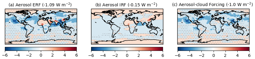
Figure 8 Changes in TOA net radiation from piClim-aer (all anthropogenic aerosols), including (a) the ERF, (b) the IRF, and (c) aerosol–cloud forcing due to ACI and the semi-direct aerosol effect. Global mean values are shown in brackets. Regions where the ERF, IRF, and the aerosol–cloud forcing are outside the 95 % confidence level are stippled. Units in W m⁻².

The SO₂ emissions are the largest individual contributor to the aerosol ERF and have a strong RA (ACI) component leading to an SO₂ (equivalent to sulfate) ERF of −1.37 ± 0.03 W m⁻² (Table 3, Fig. 7a). The IRF component of the sulfate ERF is −0.49 ± 0.01 W m⁻², which agrees well with the best estimate from AR5 (−0.40 ± 0.2 W m⁻²) and from AEROCOM Phase II (−0.58 to −0.11 W m⁻²) (Myhre et al., 2013b). The BC ERF is 0.37 ± 0.03 W m⁻², coming mostly from the IRF (0.38 ± 0.01 W m⁻²) and a small negative offset of −0.01 ± 0.02 W m⁻² from the RA term. As noted in Johnson et al. (2019), BC absorption leads to strong cloud adjustments, but the SW and LW components of these almost cancel in HadGEM3-GA7.1 and UKESM1 (see Table 3). This contrasts with many other models where the combination of low-cloud enhancements and reductions in upper-level clouds typically result in more substantial negative adjustments, making the BC ERF on average about half the magnitude of the IRF (Stjern et al., 2017). The BC ERF given by UKESM1 is however well within the range assessed by AR5 (0.05 to 0.8 W m⁻²), which took into consideration the possibility that BC emissions and/or absorption efficiency were underestimated in CMIP5 models (Bond et al., 2013). The anthropogenic emissions of BC were specified as 5 Tg yr⁻¹ in CMIP5 (year 2000 as PD) but have increased to 8 Tg yr⁻¹ in CMIP6 (year 2014 as PD). With CMIP5 emissions, the BC ERF from HadGEM3-GA7.1 was found to be 0.17 W m⁻² (Johnson et al., 2019) and is comparable to direct BC forcing from other CMIP5 model estimates (Myhre et al., 2013a). It is worth noting that the aerosol absorption was in fairly good agreement with AERONET observations in HadGEM3-GA7.1 simulations that used the CMIP5 emission set (Mulcahy et al., 2018). The slightly higher CMIP6-based estimate of 0.37 ± 0.03 W m⁻² provided in the present study could therefore be an overestimate, although this is difficult to judge given the uncertainties in comparing models with absorption measurements.

The OC ERF is −0.22 ± 0.04 W m⁻², with −0.14 ± 0.01 W m⁻² from the IRF and −0.07 ± 0.02 W m⁻² from RAs (Fig. 7a, Table 3). The OC IRF estimate agrees fairly well with AR5, which assessed the RF of primary and secondary OC to be −0.12 W m⁻² (−0.4 to 0.1 W m⁻²). Note that OC is non-absorbing in UKESM1 and, as such, neglects the role of brown carbon. This potentially misses a small positive contribution to the aerosol forcing (e.g. Feng et al., 2013), although biomass burning emissions are the dominant global source of brown carbon and these do not change significantly from 1850 to 2014 (Saleh et al., 2014). The contribution of brown carbon to aerosol ERF is, therefore, likely to be small compared to the overall uncertainty in modelling aerosol absorption by BC (Bond et al., 2013). Nitrate aerosols are also not represented in HadGEM3-GA7.1 (Mulcahy et al., 2018; Walters et al., 2019) or UKESM1 (Sellar et al., 2019; Mulcahy et al., 2020), so the ERF associated with ammonia (NH₃) emissions could not be evaluated here. The aerosol ERF in UKESM1 would presumably be more strongly negative if the role of nitrate aerosol was included (e.g. Bellouin et al., 2011) and this should be borne in mind when making comparisons with other models or estimates based on observational constraints.

The “all” aerosol forcing experiment combines the increases in BC, OC, and SO₂ emissions together in one simulation, and interestingly, the ERF is 0.13 W m⁻² weaker (less negative) than the sum of the ERFs from the experiments that perturb those emissions separately. There are three main reasons for this lack of linearity. First, cloud droplet numbers do not increase linearly with aerosol loading (e.g. Jones et al., 1994) and begin to saturate in the “all” experiment (piClim-aer), which means OC and BC emissions no longer contribute significantly to ACI once co-emitted with year-2014 levels of SO₂. Second, the absorption of upwelling SW radiation by BC is enhanced by increases in aerosol scattering and cloud brightness due to ACI, making the IRF less negative in the “all” experiment. And third, internal mixing creates an interdependency between different aerosol sources, meaning that the aerosol size distributions, optical scattering efficiency and hygroscopicity evolve differently depending on the absolute and relative abundance of different mass components (sulfate, OC, BC, and sea salt mass) and differing rates of new particle production via primary emission or nucleation.

To further understand which processes contribute most to the aerosol ERF, a series of additional control and perturbation experiments were conducted with ACI processes selectively disabled. In these tests, the cloud droplet number concentrations (CDNCs) used for the calculation of cloud droplet effective radius (Reff) and/or autoconversion were prescribed via a 3D monthly-mean PI climatology constructed from the final 30 years of the piClim-control simulation. The resulting ERFs are summarized in Fig. 7b. In one pair of simulations, CDNCs were prescribed for the Reff calculation to disable the so-called Twomey effect (Twomey, 1977). By comparison with the main piClim-aer/piClim-control experiment pair, this indicated a Twomey effect (ACI_Twomey) of −0.70 ± 0.05 W m⁻². A similar pair with CDNCs prescribed only for the autoconversion process led to an estimate of −0.31 ± 0.05 W m⁻² for the cloud lifetime effect (ACI_lifetime) (Albrecht, 1989). By prescribing CDNCs for both Reff and autoconversion, both microphysical ACI processes are disabled and only ARI are included. A pair of simulations with this setup provided an estimate for ERF_ARI of −0.15 ± 0.03 W m⁻². The change in CRE in the ARI-only experiment was only 0.02 W m⁻², which is not statistically significant at the 95 % confidence level and indicates that the semi-direct aerosol effect is small or approximately neutral in this model. To complete the breakdown, the method in Ghan (2013) was applied to the main piClim-aer/piClim-control experiment pair to derive the contribution from changes in “clean” (aerosol-free) CS radiation (RA_cs). This term was found to be 0.05 ± 0.02 W m⁻², and arises due to changes in surface albedo and atmospheric temperature and humidity. This overall breakdown suggests an aerosol–cloud forcing of −0.99 ± 0.05 W m⁻², with a roughly 70∕30 split between the Twomey effect and aerosol effects on cloud cover and water content (lifetime and semi-direct effects).

The estimated aerosol–cloud forcing sits well within the 90 % likelihood ranges assessed by AR5 (−1.2 to 0.0 W m⁻²) and Bellouin et al. (2020) (−2.0 to −0.35 W m⁻²), although these broad ranges reflect the large uncertainties involved in constraining global estimates with observations (e.g. Ghan et al., 2016). At present there are no definitive constraints on the proportionate contributions that the Twomey and other aerosol–cloud effects make towards the aerosol–cloud forcing, but recent observational evidence (Malavelle et al., 2017; Toll et al., 2017) supports the supposition that the Twomey effect is the dominant process and that some models overestimate cloud lifetime effects. Toll et al. (2017) indicated that HadGEM3 can indeed overestimate the cloud lifetime effect in marine stratocumulus, whereas Malavelle et al. (2017) found HadGEM3 to correctly simulate only weak cloud lifetime effects for mixed cloud regimes over the North Atlantic. The UKESM1 estimate of ERF_ARI of −0.15 W m⁻² is within the 5 %–95 % confidence range (−0.45 ± 0.5 W m⁻²) from AR5 but slightly weaker than the range of values estimated by Bellouin et al. (2020) (−0.60 to −0.25 W m⁻²). Possible reasons include the lack of nitrate, the relatively strong BC forcing compared to CMIP5 models, and a slight underestimation of aerosol optical depth (AOD) in PD simulations relative to some satellite products (Mulcahy et al., 2020).

4.4 Ozone (O₃) precursor (VOC, CO, and NO_x) gases

The ERF from emissions of O₃ precursors (VOC, CO, and NO_x) excluding CH₄ is weakly positive (0.21 ± 0.04 W m⁻²; Table 3; Fig. 3), although spatially heterogeneous, with sparse regions of the globe showing a statistically significant ERF (Fig. 3). O₃ precursor emissions affect the ERF both through changes in O₃, a GHG, and by changing tropospheric oxidants such as the hydroxyl (OH) radical, which in turn affect aerosols (Karset et al., 2018) and CH₄ lifetime. Here, we explore the composition and forcings resulting from O₃ precursor emission changes by comparing the piClim-O3 simulation with piClim-control (Table 1) and the separate effects of NO_x and VOC ∕ CO emission changes using the piClim-NOx and piClim-VOC simulations, respectively.

4.4.1 Tropospheric ozone (O₃) changes

The tropospheric O₃ column for the piClim-control simulation, and tropospheric O₃ column differences between piClim-control and the piClim-O3, piClim-NOx, and piClim-VOC simulations are shown in Fig. 9. O₃ levels in the troposphere are the result of competing production and loss processes. Production occurs in the presence of NO_x and VOC ∕ CO, with most regions of the troposphere being NO_x-limited. PI tropospheric column O₃ values (Fig. 9a) show maxima over central Africa and the eastern tropical Pacific, the result of relatively large emissions of NO_x from soil, biomass burning, and lightning in this region, and minima over regions remote from NO_x sources, such as the western equatorial Pacific (where O₃ loss is efficient), consistent with Young et al. (2018). Tropospheric column O₃ is also low over regions of high surface elevation where the atmospheric column is shallower.

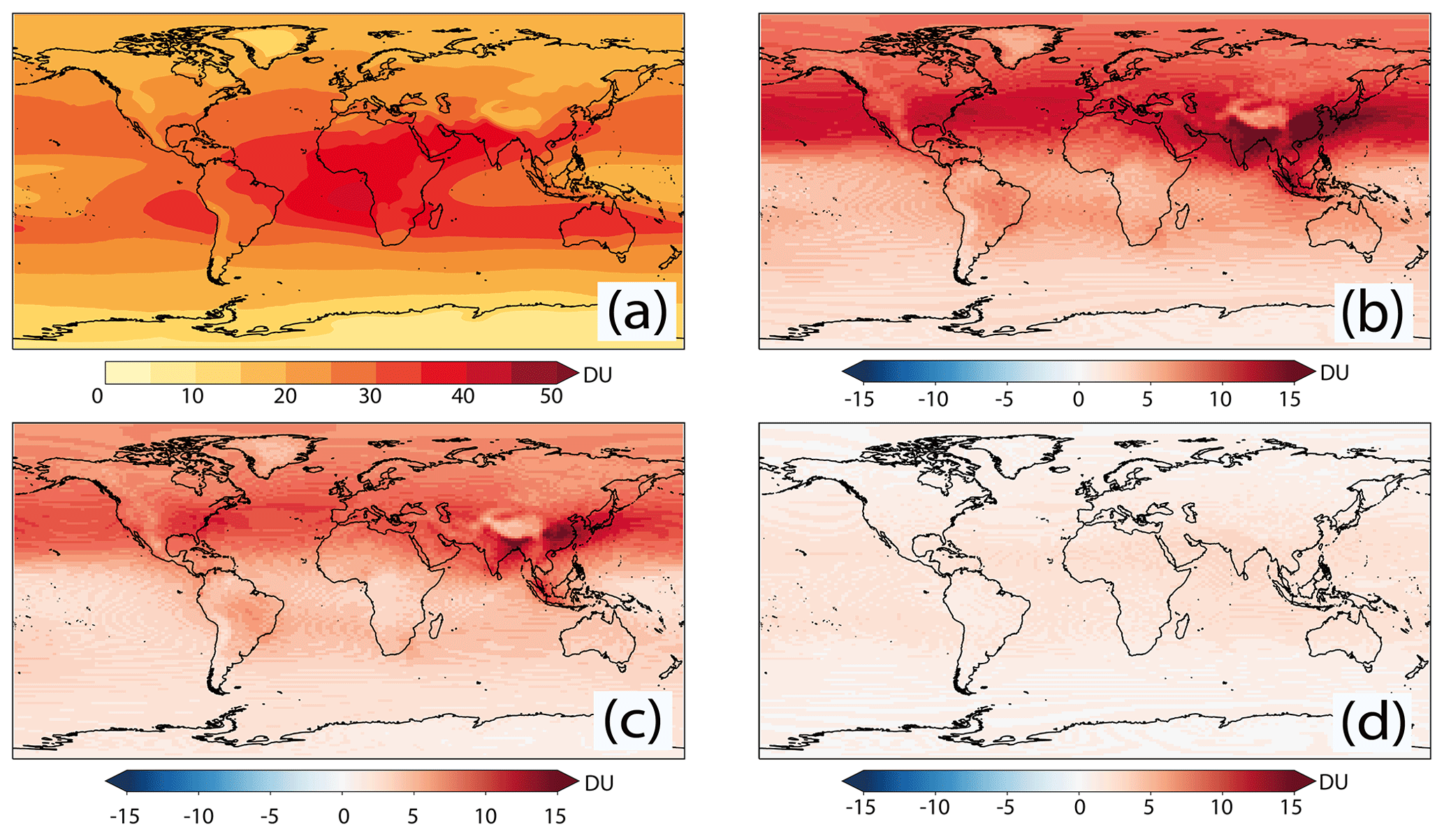
Figure 9 Global distributions of tropospheric O₃ column (a) in piClim-control. Differences with respect to piClim-control from piClim-O3, piClim-NOx and piClim-VOC can be seen in panels (b), (c), and (d), respectively. Units in Dobson units (DU).

Tropospheric O₃ column values increase when the model is perturbed with the larger PD O₃ precursor emissions in piClim-O3, with the largest increases in the NH, particularly in southern and eastern Asia. The tropospheric O₃ burden increases from 280.9 Tg in piClim-control to 355.5 Tg in piClim-O3. As can be seen in Fig. 9, the dominant driver of these changes are increased NO_x emissions, and there is a similar pattern of changes in the piClim-O3 and piClim-NOx simulations, although the change in O₃ is smaller in the latter; the burden in piClim-NOx is 337.5 Tg. Small increases in O₃ are modelled in piClim-VOC, with some hotspots in regions such as South East Asia and the O₃ burden increases to 296.8 Tg.

The tropospheric O₃ burden difference between piClim-O3 and piClim-control of 74.6 Tg is slightly larger than the sum of the individual O₃ burden changes in piClim-NOx (56.6 Tg) and piClim-VOC (15.9 Tg), which total 72.5 Tg. However, these differences due to the non-linear nature of tropospheric chemistry are small, being on the order of <5 %. Similar behaviour is seen in the patterns of the tropospheric O₃ column difference between piClim-control and other experiments.

4.4.2 Tropospheric O₃ stratospherically adjusted radiative forcing (SARF)

As seen in earlier sections, it can be difficult to compare ERFs estimated from these experiments against estimates of SARF (e.g. Stevenson et al., 2013; Myhre et al., 2013a), due to the inclusion of indirect forcings and/or RAs other than the stratospheric temperature adjustment, although Shindell et al. (2013b) and Skeie et al. (2020) noted that for O₃, SARF and ERF estimates are comparable. Nevertheless, in order to compare against Stevenson et al. (2013), we estimate the tropospheric O₃ SARF from the piClim-CH4, piClim-VOC, and the piClim-NOx experiments by adopting a radiative kernel approach (e.g. Soden et al., 2008). This involves applying the tropospheric O₃ radiative kernel from Rap et al. (2015) to the diagnosed change in tropospheric O₃ (using the 150 ppbv O₃ isoline in piClim-control as a tropospheric mask, as used in Young et al., 2013; Stevenson et al., 2013; Rap et al., 2015) to calculate a SARF. While the ERF captures changes in radiative fluxes at the TOA due to whole-atmosphere responses, here we mask off the stratosphere and focus solely on the tropospheric O₃ response. In this way, we can directly compare against the best estimate of the 1850–2010 tropospheric O₃ SARF of 364 mW m⁻² by Stevenson et al. (2013) and quantify the contribution of different O₃ precursors (including CH₄) to the change in tropospheric O₃ and its SARF. We can also compare with more recent estimates from Checa-Garcia et al. (2018) and Yeung et al. (2019).

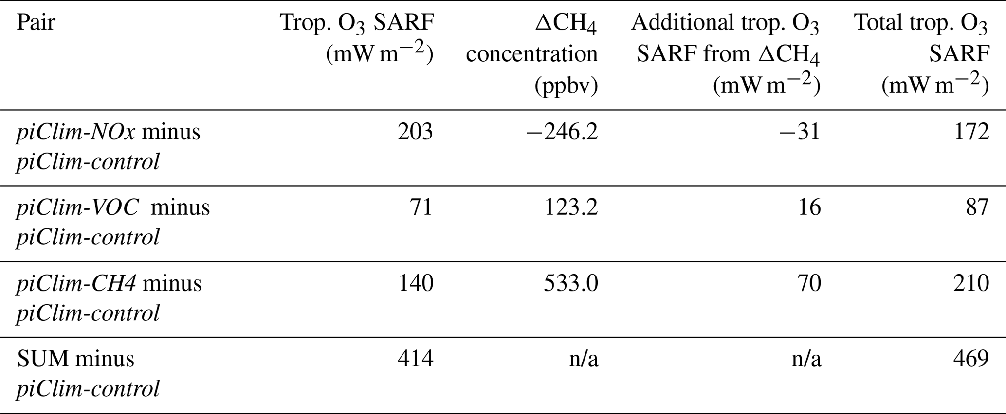
Figure 10 shows the global distribution of the tropospheric O₃ SARF from piClim-CH4, piClim-NOx, and piClim-VOC experiments and their sum using the kernel approach. It shows that the tropospheric O₃ SARF is strongest over the NH sub-tropics and weakest over the SH high latitudes. The strongest SARF occurs in regions of warm surface temperatures and high albedo, coinciding with the largest tropospheric O₃ change (Shindell et al., 2013a). As was the case in Stevenson et al. (2013), the SARF is weaker over regions of high altitude (e.g. the Tibetan Plateau) due to there being less O₃ column aloft to absorb in the LW. The tropospheric O₃ SARF from the kernel approach is 414 mW m⁻². However, the increase in tropospheric O₃ (and its resulting SARF) are offset by decreases due to ODSs (e.g. Søvde et al., 2011, 2012; Shindell et al., 2013a). Applying the kernel method to the diagnosed decrease in tropospheric O₃ from the piClim-HC experiment (Sect. 4.2.3), we find a SARF offset of −101 mW m⁻². Although larger in magnitude by nearly a factor of 2 than the estimates from Søvde et al. (2011, 2012) and Shindell et al. (2013a) due to the strong O₃ depletion in UKESM1 (Keeble et al., 2020; Skeie et al., 2020; Morgenstern et al., 2020), it reduces our original estimate to 313 mW m⁻². This revised estimate is within the 30 % uncertainty of the Stevenson et al. (2013) estimate, albeit lower than their central estimate by 13 %. It is also consistent with a number of other estimates: the CMIP6 historical O₃ dataset (312 mW m⁻² from Checa-Garcia et al., 2018), a recent study in which observational isotopic data was used as a constraint on historical increases in tropospheric O₃ (330 mW m⁻² derived from the GEOSChem model in Yeung et al., 2019), and a parametric model based on multi-model source–receptor relationships (290 ± 3 mW m⁻² from Turnock et al., 2019). However, in masking off the stratosphere, the UKESM1 estimate for the O₃ SARF attributable to O₃ precursors is likely to be underestimated. For example, Søvde et al. (2011, 2012) estimate that approximately 15 % of the O₃ response from changes in CH₄ and other O₃ precursors may be in the stratosphere and hence not considered here.

Table 5 Contribution to the tropospheric O₃ SARF from the different perturbation experiments (piClim-NOx, piClim-VOC, and piClim-CH4) relative to the pre-industrial control (piClim-control). Also shown is the absolute difference between the equilibrium and prescribed CH₄ concentrations in the different experiments and the resulting additional contribution to the total tropospheric O₃ SARF from the CH₄-driven response in O₃.

n/a: not applicable.

In considering the attribution of the tropospheric O₃ SARF to its precursors, initial estimates (Fig. 10; Table 5) indicate that it is predominantly NO_x driven (49 %), followed by CH₄ (34 %), with the smallest contribution from VOCs and CO (17 %). This is qualitatively consistent with Stevenson et al. (2013). However, as outlined in detail in that paper, these estimates do not account for potential CH₄ (and O₃) changes that would occur if these experiments were driven by CH₄ emissions rather than concentrations (e.g. Shindell et al., 2005). Taking the same approach as Stevenson et al. (2013), we calculate an equilibrium CH₄ concentration for the perturbation experiments using the total CH₄ lifetime relative to piClim-control based on the following (Fiore et al., 2009):

$$\begin{array}{}\text{(9)}& \begin{array}{rl}{\left[{\mathrm{CH}}_{\mathrm{4}}\right]}_{\mathit{piClim}-X}& ={\left[{\mathrm{CH}}_{\mathrm{4}}\right]}_{\mathit{piClim}-\mathit{control}}\\ & \cdot {\left({\displaystyle \frac{{\mathit{\tau }}_{\mathit{piClim}-X}}{{\mathit{\tau }}_{\mathit{piClim}-\mathit{control}}}}\right)}^f,\end{array}\end{array}$$

where ${\left[{\mathrm{CH}}_{\mathrm{4}}\right]}_{\mathit{piClim}-X}$ is the global mean equilibrium CH₄ concentration in the piClim-X experiments, ${\left[{\mathrm{CH}}_{\mathrm{4}}\right]}_{\mathit{piClim}-\mathit{control}}$ is the prescribed global mean CH₄ concentration in piClim-control, and τ_{piClim−control} and τ_piClim−X are the whole-atmosphere CH₄ lifetimes in the piClim-control and piClim-X perturbation experiments, respectively. The CH₄–OH feedback factor (Prather, 1996) is denoted by f and is defined as

$$\begin{array}{}\text{(10)}& f={\displaystyle \frac{\mathrm{1}}{\mathrm{1}-s}},\end{array}$$

where s, called the sensitivity coefficient, is calculated from the following:

$$\begin{array}{}\text{(11)}& s={\displaystyle \frac{\mathit{\delta }\ln \mathit{\tau }}{\mathit{\delta }\ln \left[{\mathrm{CH}}_{\mathrm{4}}\right]}}.\end{array}$$

Using the whole-atmosphere CH₄ burden and its removal by OH, the whole-atmosphere CH₄ lifetime is 8.1 and 9.8 years in piClim-control and piClim-CH4, respectively, when adjusted for stratospheric removal (120 years lifetime) and soil uptake (160 years lifetime). From Eqs. (10) and (11), the UKESM1 feedback factor f is 1.28, consistent with the range of other estimates (Prather et al., 2001; Shindell et al., 2005; Fiore et al., 2009; Stevenson et al., 2013; Voulgarakis et al., 2013; Turnock et al., 2018) and within 5 % of the observationally constrained best estimate of 1.34 (Holmes et al., 2013). Then, using the equilibrium minus prescribed difference in surface CH₄ concentrations (Table 5), we calculate the additional tropospheric O₃ SARF in the piClim-CH4, piClim-NOx, and piClim-VOC experiments by applying the tropospheric O₃ radiative kernel (Rap et al., 2015) to the O₃ response derived from scaling the (piClim-CH4 minus piClim-control) O₃ response based on the relationship in Turnock et al. (2018); these additional contributions to the tropospheric O₃ SARF are shown in Table 5.

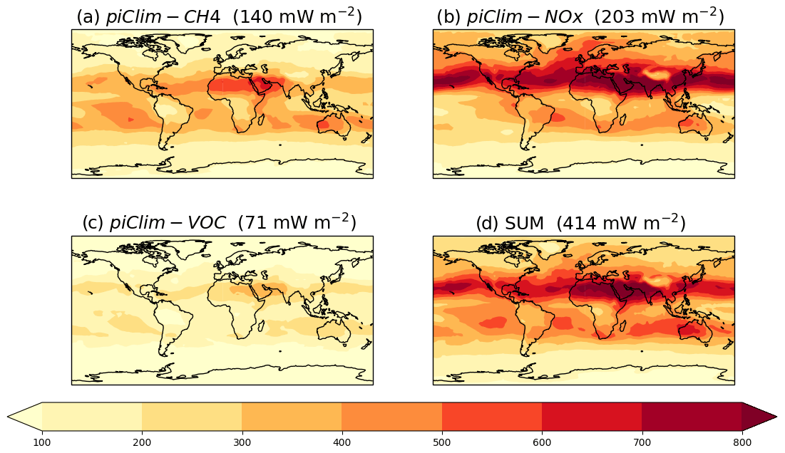
Figure 10 Global distribution of tropospheric O₃ SARF diagnosed from (a) piClim-CH4, (b) piClim-NOx, (c) piClim-VOC, and (d) their sum relative to piClim-control, based on the diagnosed change in tropospheric O₃ and the tropospheric O₃ radiative kernel of Rap et al. (2015). Global mean values are included. Units in mW m⁻².

Changing from a concentration-based perspective to an emissions-based view increases the tropospheric O₃ SARF from 414 to 469 mW m⁻² (an increase of 13 %), which agrees better with the central estimate from Stevenson et al. (2013) once the offset by ODSs is accounted for (−101 mW m⁻²). It also changes the relative contributions of the different O₃ precursors. The contribution of CH₄ now dominates (45 %), with NO_x playing a smaller role (37 %), while the contribution from VOC ∕ CO emission increases is relatively unchanged (18 %). These emissions-based contributions are well within the spread of estimates from Stevenson et al. (2013), who quantified contributions from six of the ACCMIP models: CH₄ (44 ± 12 %), NO_x (31 ± 9 %), and VOC ∕ CO (25 ± 3 %) although there are some differences with Shindell et al. (2005) and Shindell et al. (2009). In both Shindell et al. studies, the contribution from NO_x is lower at 15 ± 8 and 11 %. The difference may be due to the strong sensitivity of the CH₄ lifetime to NO_x in the GISS model compared with other models (Wild et al., 2020) and/or could be due to differences in VOC chemistry; Archibald et al. (2010) showed that the response of OH to increasing NO_x strongly depends on the treatment of VOC chemistry. Nevertheless, this approach demonstrates the importance of an emissions-based view of climate forcing and is more directly relevant to policy makers than a concentration-based view (Shindell et al., 2005, 2009).

4.4.3 ERF: role of other oxidants and aerosols

In addition to O₃ being a GHG, it is also important for secondary aerosol formation along with other oxidants: the OH radical, hydrogen peroxide (H₂O₂), and the nitrate (NO₃) radical. The OH radical in UKESM1 (Sellar et al., 2019) is involved in aerosol nucleation of gas-phase sulfuric acid (H₂SO₄) via the reaction with sulfur dioxide (SO₂), leading to new particle formation (Mulcahy et al., 2020). O₃ and H₂O₂ are important for SO₂ oxidation in cloud and aerosol droplets, creating sulfate aerosol mass but not number. Likewise, oxidation of monoterpenes by O₃, OH, and NO₃ determines the rate of formation of secondary organic aerosol (SOA) in UKESM1 (Kelly et al., 2018; Mulcahy et al., 2020) although it does not lead to new particle formation. Thus, sulfate aerosol alone, through changes in O₃, OH, and H₂O₂, has potentially important impacts on cloud and aerosol radiative properties. Indeed, Karset et al. (2018) found that oxidant changes in the CAM5.3-Oslo model alter the relative importance of different chemical reactions, leading to changes in aerosol size distribution, cloud condensation nuclei (CCN), and the aerosol ERF.

Figure 11 (bottom row) shows a global distribution of OH at 1 km altitude in piClim-control and changes in the perturbation experiments relative to piClim-control. The piClim-control experiment shows an OH maximum in the equatorial humid regions, where photolytic production of OH from excited oxygen atoms (O¹D) and water vapour (H₂O) is at a maximum. In piClim-O3, OH increases throughout the NH due to increases in O₃, which is the precursor of O¹D. These increases in OH are driven largely by increases in NO_x. However, the piClim-VOC experiment shows the opposite behaviour. While VOC and CO emission increases serve to increase O₃, they also remove OH via direct reaction with OH. This latter effect outweighs the small increase in O₃ in piClim-VOC and there are decreases in OH throughout the troposphere.

When OH is lower, we anticipate a decrease in the number of CCN and a decrease in CDNC, leading to larger cloud droplets (Twomey, 1977) and an increase in Reff. The middle rows of Fig. 11 show these effects at work. In piClim-control, the distribution of CDNC shows large values in equatorial regions, regions of continental outflow, and regions of deep convection. Large increases in CDNC are seen in piClim-NOx with large decreases in piClim-VOC. These results reflect the changes in OH in these experiments. Increases in OH lead to increases in CDNC, and vice versa, but it should be noted that the effect of OH on CDNC is seen over a larger region downwind, particularly in East Asia and over the North Atlantic. The impact of NO_x emissions appears to dominate, given the similarity between piClim-O3 and piClim-NOx.

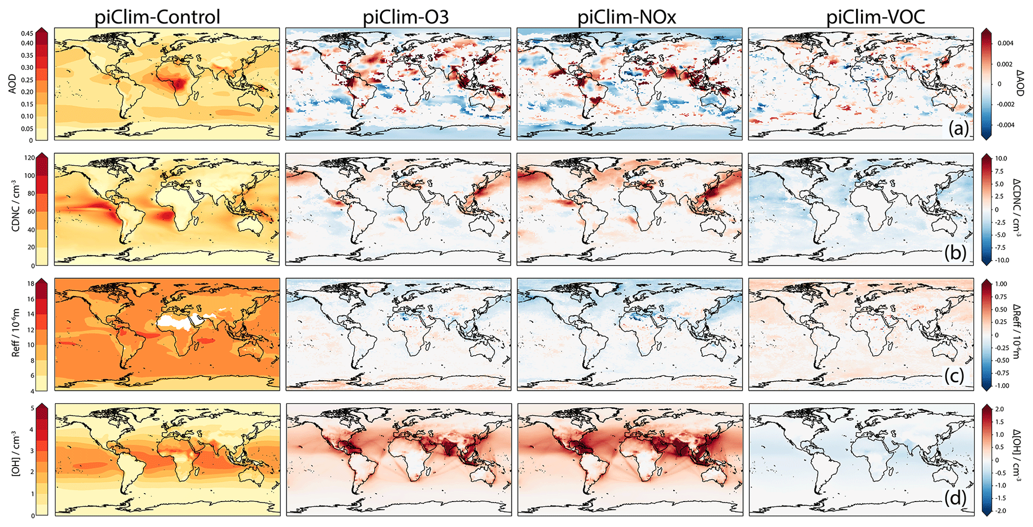
Figure 11 Global distributions of AOD at 550 nm (row a; left column), cloud droplet number concentration (CDNC; cm⁻³) at 1 km altitude (row b; left column), cloud droplet effective radius (Reff; µm) at 1 km altitude (row c; left column), and OH number concentration (cm⁻³) at 1 km altitude (row d; left column) in piClim-control. Differences with respect to piClim-control from piClim-O3, piClim-NOx, and piClim-VOC can be seen in the second, third, and right-hand columns, respectively.

While tropospheric column O₃ increases in both piClim-NOx and piClim-VOC, leading to positive contributions to the tropospheric O₃ SARF (Sect. 4.4.2), the ERFs are very different between the two simulations (0.33 ± 0.04 W m⁻² for piClim-VOC and 0.03 ± 0.04 W m⁻² for piClim-NOx relative to piClim-control). Further, the spatial pattern of the ERF does not match those regions of largest O₃ changes. Instead, the dominant driver of the ERF differences are changes to OH and the subsequent impacts on aerosol particle formation and clouds. In particular, the positive tropospheric O₃ SARF in piClim-NOx (0.2 W m⁻², Table 5) appears to be nearly completely offset by a negative aerosol forcing, largely from ACI driven by changes in oxidants and aerosol nucleation; the contribution to the global mean ERF from ARI is only −0.03 ± 0.01 W m⁻², despite the strong regional changes in AOD at 550 nm (Fig. 11; top row). Similarly, the aerosol IRF in piClim-VOC is negligible (less than 0.01 ± 0.01 W m⁻²). However, the forcing in piClim-VOC due to ACI, particularly from the SW ΔCRE^′ component (Table 3), enhances the positive tropospheric O₃ SARF (0.07 W m⁻²), leading to an ERF of 0.33 ± 0.04 W m⁻².

A negative SARF attributable to NO_x emissions has been found in other studies (Shindell et al., 2009; Collins et al., 2010) from a balance between the direct O₃ response (positive SARF), the NO_x-driven CH₄ response (negative SARF), and the subsequent O₃ response to CH₄ changes (negative SARF). Inclusion of ARI and ACI from sulfate and nitrate aerosol further increases the magnitude of the net negative forcing or cooling (Shindell et al., 2009; Collins et al., 2010). However, a study by Fry et al. (2012) found that the chemistry response is sensitive to the location of the emissions, with so large an uncertainty that it is difficult to determine whether NO_x emissions cause a warming or cooling. Indeed, other indirect effects such as NO_x deposition to the terrestrial biosphere leading to fertilization (Collins et al., 2010) and/or NO_x-driven O₃ damage (Sitch et al., 2007; Collins et al., 2010) increase the uncertainty further through changes in CO₂. Thornhill et al. (2020) show that the ERF from changes in NO_x emissions among the AerChemMIP models differ in both sign and magnitude. Here, the longer timescale CH₄ response to NO_x emissions (Collins et al., 2010) is constrained, nitrate aerosol is neglected (Sellar et al., 2019; Mulcahy et al., 2020), and CO₂ is concentration-driven (Sellar et al., 2019). Nevertheless, in UKESM1, the negative forcing due to ACI from sulfate aerosol offsets the positive NO_x-driven O₃ SARF, leading to a negligible ERF overall.

Previous work has also found a positive SARF from VOC and CO emissions, due to the combined indirect forcings by O₃ and CH₄ (Shindell et al., 2005; Forster et al., 2007); they estimate a global mean SARF of 0.21 ± 0.10 W m⁻² at the PD (year 1998) relative to the PI (year 1750) period. Via the same mechanisms as was the case with NO_x, the magnitude of this SARF increases (to 0.25 ± 0.04 W m⁻² for the year 2000) when additional indirect forcings from sulfate, nitrate, and CO₂ are included (Shindell et al., 2009). More recently, Stevenson et al. (2013) found the SARF from VOC ∕ CO emissions to be marginally higher, at 0.29 W m⁻², excluding aerosols, with contributions of 0.09, 0.08, and 0.12 W m⁻² from O₃, CH₄, and CO₂, respectively. The SARF contribution from O₃ alone quantified here (87 mW m⁻²; Table 5) is consistent with the Stevenson et al. (2013) estimate. Despite excluding the longer-term CH₄ and CO₂ responses, the ERF from VOC ∕ CO emissions of 0.33 ± 0.03 W m⁻² is higher than previous estimates of SARF due to the additional positive contribution from ACI driven by OH changes. However, Fry et al. (2014) found that the SARF from VOCs is sensitive to the location of emissions and could influence the strength of the contribution from aerosols. Interestingly, other AerChemMIP models show a negative ERF from VOC and CO emissions (Thornhill et al., 2020); these differences in sign of the ERF warrant further investigation.

As a result of the very different chemical response between NO_x and VOC ∕ CO emissions, both in terms of the magnitude of the O₃ changes and the different impacts on OH, aerosols, and clouds, a comparison of the ERFs (Table 3) indicates that the ERF from piClim-O3 is not a linear combination of that from piClim-NOx and piClim-VOC for the NET, CS, and CRE components. In particular, there are differences in the LW${}_{\mathrm{cs}}^{\prime }$ and SW ΔCRE^′ components (Table 3). These results clearly suggest that Earth system (ES) interactions, particularly chemistry–aerosol coupling, can strongly affect estimates of climate forcing. Here, these interactions alter the ERF from O₃ precursor emissions, while other studies (e.g. Shindell et al., 2009; Karset et al., 2018) show that they also affect estimates of anthropogenic aerosol forcing.

4.5 Other forcings

4.5.1 Non-methane near-term climate forcers (NTCFs)

The anthropogenic ERF due to CH₄, aerosols, and O₃ abundances was identified as the main source of uncertainty in the total anthropogenic ERF since PI times (Myhre et al., 2013a). This is due to the uncertainty in the individual forcings (e.g. Bellouin et al., 2020), but the interaction between individual forcings as well as the non-linear response of climate feedbacks due to ACI (Feichter et al., 2004; Deng et al., 2016; Collins et al., 2017; Shim et al., 2019) may play a role. In this section, three experiments related to non-CH₄ NTCFs are discussed: (1) the combined simulation (piClim-NTCF), which is identical to piClim-control except that aerosol and O₃ precursor emissions are set to PD (year 2014) levels, (2) piClim-aer, which changes aerosol and aerosol precursor emissions only , and (3) piClim-O3 which changes O₃ precursor (VOC, CO, NO_x) emissions only from PI to PD levels. More details are described in Table 1.

The ERF of non-CH₄ NTCFs is −1.03 ± 0.04 W m⁻² (Table 3; Fig. 12). The negative ERF results from the combination of a weak negative NET${}_{\mathrm{cs}}^{\prime }$ component (−0.03 ± 0.03 W m⁻²) and a strong contribution due to the NET CRE^′ component (−1.00 ± 0.02 W m⁻²). The weak negative contribution in the CS (NET${}_{\mathrm{cs}}^{\prime }$) is due to the negative SW${}_{\mathrm{cs}}^{\prime }$ component (−0.26 ± 0.02 W m⁻²) being largely offset by the positive LW${}_{\mathrm{cs}}^{\prime }$ component (0.23 ± 0.03 W m⁻²). The negative SW${}_{\mathrm{cs}}^{\prime }$ component is correlated with changes in AOD at 550 nm (spatial correlation coefficient of −0.44) and is predominantly due to the aerosol IRF (−0.29 ± 0.01 W m⁻²). The LW${}_{\mathrm{cs}}^{\prime }$ component is positive (0.23 ± 0.03 W m⁻²) due to both aerosols and O_3, but with the aerosol IRF only contributing 0.04 ± 0.01 W m⁻². The spatial variations in the global distribution of the LW${}_{\mathrm{cs}}^{\prime }$ component are closely related to land surface temperature (T_s) changes; the correlation coefficient is −0.78 with a statistical significance well over 99 %. Considering this good correlation, the increased LW${}_{\mathrm{cs}}^{\prime }$ component is in response to the T_s change due to NTCFs. The negative SW ΔCRE^′ component (−0.92 ± 0.03 W m⁻²), however, dominates the ERF and is largely correlated with changes in cloudiness, with the spatial pattern correlation of −0.59 between the SW ΔCRE^′ component and cloud fraction.

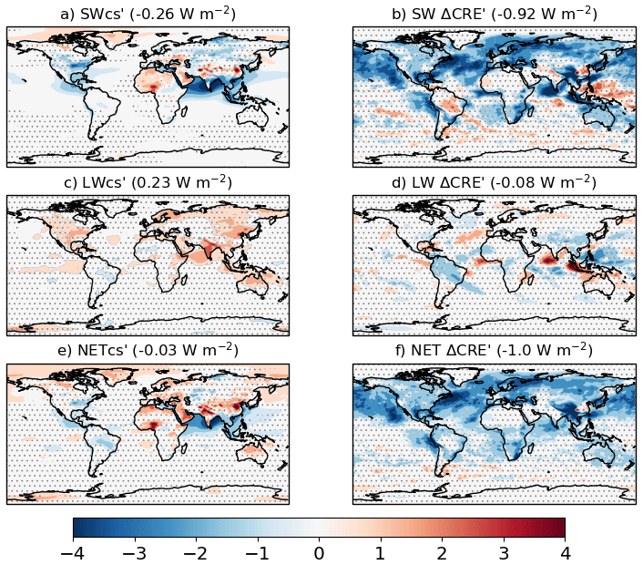
Figure 12 Global distributions of the PD NTCF ERF components at the top of atmosphere (TOA) relative to the PI period, i.e. piClim-NTCF minus piClim-control, based on Eq. (8): (a) SW${}_{\mathrm{cs}}^{\prime }$, (b) SW CRE^′, (c) LW${}_{\mathrm{cs}}^{\prime }$, (d) LW CRE^′, (e) NET${}_{\mathrm{cs}}^{\prime }$, and (f) NET CRE^′. Global mean values are shown in brackets. Regions where the ERF components are outside the 95 % confidence level are stippled. Units in W m⁻².

As was the case for other ERFs (e.g. GHGs, aerosols, and O₃ precursor gases), the range of perturbation simulations carried out with UKESM1 enables the role of non-linear interactions to be investigated. The total GHG ERF was found to be equal to the sum of the individual GHG ERFs (Sect. 4.2.5) but non-linearities were evident for the aerosol (Sect. 4.3) and the O₃ precursor (Sect. 4.4) ERFs. As a result, this study also attempts to estimate the effects of the non-linear interactions between chemistry and aerosols on the combined aerosol and O₃ precursor ERF. When combined (aerosol and aerosol precursor, and O₃ precursor emissions), their interaction may induce an effect that differs from the sum of the individual single ERFs. The ERFs do not add linearly, particularly in the SW${}_{\mathrm{cs}}^{\prime }$ and NET CRE' components (Table 3). Firstly, we calculate the aerosol IRFs using Eq. (7). In piClim-NTCF, the net (SW + LW) aerosol IRF is −0.24 ± 0.01 W m⁻², which is more negative than the sum of the aerosol IRF in piClim-aer (−0.15 ± 0.01 W m⁻²) and piClim-O3 (−0.02 ± 0.01 W m⁻²). This is due to the sulfate aerosol loading being higher in piClim-NTCF relative to piClim-aer by up to 3.4 (27) % globally (regionally), and driven by changes in oxidants due to the PD levels of O₃ precursors. Secondly, the NET CRE^′ component contributes to the non-linearity in the ERFs. The NET CRE^′ component is more negative in piClim-NTCF (−1.00 ± 0.02 W m⁻²) than in the sum of piClim-aer (−1.0 ± 0.02 W m⁻²) and piClim-O3 (0.08 ± 0.02 W m⁻²). This is primarily the result of differences in the SW ΔCRE^′ component, again driven by the higher sulfate loading in piClim-NTCF relative to piClim-aer.

Although there is no direct coupling between aerosols and photolysis in UKESM1 (Archibald et al., 2020), aerosol-mediated cloud adjustments result in SW reduction and surface cooling. These changes impact thermal and photochemical reactions leading to reduced photolysis rates (O₃+ hν→ O(¹D) + O₂) in the lower troposphere, while enhancing the photolysis rate of O₃ in the upper troposphere (black and blue dotted lines in Fig. 13), leading to a reduction in surface O₃ in piClim-NTCF relative to the sum. However, despite differences in O₃ (not shown), the LW${}_{\mathrm{cs}}^{\prime }$ components of the ERFs appear to add linearly.

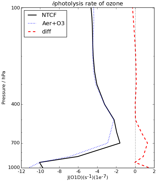
Figure 13 Vertical distribution of changes in j(O¹D) photolysis rates (10⁻⁷ s⁻¹) in piClim-NTCF (black solid line), the sum (blue dotted line) of piClim-aer and piClim-O3 relative to piClim-control, and the difference between them (red dashed line).

4.5.2 Land use

LU change causes RF primarily by changing surface albedo; croplands and pastures have higher albedos than forests and are less able to mask the high albedo of snow cover. Increased albedo leads to a negative SW${}_{\mathrm{cs}}^{\prime }$ component (−0.30 ± 0.02 W m⁻²; Table 3) that is damped by the SW CRE^′ (0.09 ± 0.03 W m⁻²; Table 3), and the inclusion of small positive LW${}_{\mathrm{cs}}^{\prime }$ (0.02 ± 0.03 W m⁻²; Table 3) and LW CRE^′ (0.03 ± 0.01 W m⁻²; Table 3) terms leads to a net ERF of −0.17 ± 0.04 W m⁻². The LU ERF of UKESM1 is close to being within the “very likely” range (−0.15 to −0.10 W m⁻²) of AR5 (Myhre et al., 2013a). However, the AR5 estimate is valid for LU change since 1700, not 1850 as in our estimate. Andrews et al. (2017) used HadGEM2-ES, UKESM1's predecessor, to calculate a 1700–1860 LU ERF of −0.1 W m⁻². If we apply this adjustment to our estimate, we find an ERF of −0.27 W m⁻², which is well outside of the AR5 range. The UKESM1 LU ERF (−0.17 ± 0.04 W m⁻²) is reduced relative to HadGEM2-ES, which produced an 1860–2005 LU ERF of −0.40 W m⁻² (Andrews et al., 2017). Robertson (2019) showed that, even in the absence of snow cover, the albedo response to LU change in HadGEM2-ES is stronger than observed; at the location of deforestation, the surface SW response to total deforestation was generally 5 W m⁻² too large. It is likely that the bias found in HadGEM2-ES still exists in UKESM1.

While the global mean LU ERF is small, regionally it can be the dominant source of the anthropogenic ERF. Figure 14 shows the distribution of the LU ERF and its cloud-free and aerosol-free component, which emphasizes the surface flux contribution. The ERF is mostly confined to regions of LU change, with deforestation in North America and western Eurasia causing a negative ERF and increased tree cover in central Europe causing a positive ERF. Alongside the distribution of LU change itself, the magnitude of the ERF is larger in the mid-latitudes than the tropics, because the masking of snow cover by trees greatly increases the albedo response to changes in tree cover. The large regions of negative ERF in the northern mid-latitudes are consistent with previous model studies (e.g. de Noblet-Ducoudre et al., 2012); they are caused by agricultural expansion and the forcing is expected to have gradually increased over the period 1850–1970 in North America and over the period 1900–1980 in Eurasia. The seasonality of leafiness, snow cover and insolation causes the LU ERF to be largest in NH spring (March to May mean of −0.28 ± 0.11 W m⁻²) and smallest in autumn (September to November mean of −0.08 ± 0.09 W m⁻²).

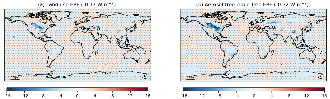
Figure 14 Global distribution of the present-day (PD; year 2014) ERF relative to the pre-industrial (PI; year 1850) period of (a) LU ERF and (b) the contribution from the cloud-free and aerosol-free component. Global mean values are included and areas are stippled where the ERF and/or its component are not statistically significant from zero at the 95 % confidence interval. Units in W m⁻².

The LU ERF is calculated by modifying three land surface fields: land cover, LAI, and canopy height. The values of the modified fields are taken from a coupled UKESM1 simulation that is only subject to historical LU change. In the coupled configuration of UKESM1 (Sellar et al., 2019), the three land surface fields are prognostic fields calculated using a dynamic global vegetation model (DGVM), while in the atmosphere-only ERF configuration they are prescribed fields. This choice was made because the land surface fields can be very slow to respond to changes in land use and RF. In the coupled simulation of historical climate change including all forcings (historical), the land surface fields respond to changes in CO₂, climate, and land use, but if we use the land surface fields from this simulation, we find no substantial change in the LU ERF (−0.20 W m⁻²).

In addition to the ERF caused by albedo changes, LU change can alter climate via a number of other mechanisms. LU change alters the land carbon sink. In particular, deforestation emits CO₂ to the atmosphere, and so some fraction of the CO₂ ERF is attributable to LU change. LU change also affects surface climate via changes in roughness length and transpiration. These non-radiative mechanisms usually drive larger temperature changes than the albedo response and both the non-radiative mechanisms and the CO₂ forcings tend to oppose the albedo response.

4.5.3 Total anthropogenic ERF

As noted above, historical climate change has been driven by a wide range of anthropogenic activities that act together, alongside natural changes, to perturb the Earth's radiation balance. The total anthropogenic ERF is, therefore, a key metric in understanding observed and modelled changes in the climate system since the PI era. These various anthropogenic drivers are not necessarily independent of each other and it is therefore worthwhile to calculate the total anthropogenic ERF from a separate time slice simulation including all perturbations together (piClim-anthro; Pincus et al., 2016). We completed a dedicated time slice simulation with all concentrations, emissions, and land use set to 2014 levels, including all GHG concentrations (CO₂, N₂O, CH₄, HCs – both ODSs and non-ODSs), O₃ precursors (VOC, CO, NO_x), LU changes, and anthropogenic aerosol or aerosol precursor emissions (SO₂, OC, BC). This experiment was not proposed in AerChemMIP (Collins et al., 2017) but is included here as part of RFMIP (Pincus et al., 2016). The main difference is that atmospheric chemistry in UKESM1 is fully interactive whereas other models participating in RFMIP (e.g. Andrews et al., 2019) use the CMIP6 O₃ dataset to represent changes in tropospheric and stratospheric O₃ and prescribe oxidants for secondary aerosol formation.

The UKESM1 piClim-anthro experiment leads to an ERF of 1.76 ± 0.04 W m⁻² (Table 3), which is dominated by a positive LW${}_{\mathrm{cs}}^{\prime }$ component due to GHGs and partially offset by a negative SW${}_{\mathrm{cs}}^{\prime }$ component due to aerosols and negative contributions from the SW ΔCRE^′ and LW ΔCRE^′ components (Table 3). This ERF is a little lower than the equivalent estimate from HadGEM3-GA7.1, which was 1.81 W m⁻² (Andrews et al., 2019). The UKESM1 estimate is also lower than the median estimate from CMIP5 models assessed in AR5, which equates to approximately 1.9 W m⁻² after adjustment to the reference period of 1861–1880 to 2010–2011 (Andrews and Forster, 2020). AR5 also provided an overall central estimate of 2.2 W m⁻² and a 5 %–95 % confidence range of 1.0 to 3.2 W m⁻² (after adjustment to the same reference period as above in Andrews and Forster, 2020) taking into account multiple streams of evidence. Andrews and Forster (2020) re-evaluated this as 2.3 W m⁻² with a narrower range of 1.7–3.0 W m⁻² [5 %–95 % confidence] using a combination of atmospheric model outputs and observational constraints. The lower bound of this range was reduced to 1.5 W m⁻² if larger uncertainties were assumed for the climate feedback parameter or for the global-mean surface temperatures anomalies used to constrain the forcing. The UKESM1 estimate of 1.76 ± 0.04 W m⁻² is therefore within the original uncertainty range given by AR5 and just within the range proposed in Andrews and Forster (2020).

There are several factors that contribute to the relatively low estimate of anthropogenic ERF in UKESM1. Firstly, the anthropogenic aerosol ERF in UKESM1 (and HadGEM3-GC3.1) is −1.09 ± 0.04 W m⁻² (well within the uncertainty range of Bellouin et al., 2020) and offsets a major portion of the positive GHG ERF (2.92 ± 0.04 W m⁻²). Secondly, the ERF from piClim-HC is negative (−0.18 ± 0.04 W m⁻²) due to a strong O₃ response and connected aerosol-mediated cloud adjustments (Morgenstern et al., 2020). Thirdly, adjustments in vegetation lead to an appreciable negative ERF from LU changes (−0.17 ± 0.04 W m⁻²). The stronger negative ERF from piClim-HC balanced by a stronger positive ERF from piClim-CH4 (0.97 ± 0.04 W m⁻²) due to indirect effects and the positive tropospheric RA term (Thornhill et al., 2020) largely explain why the UKESM1 estimate is only ∼ 0.05 W m⁻² lower than HadGEM3-GA7.1. As shown in Fig. 3i, the negative contributions more than offset the positive GHG ERF in certain regions. For instance, the anthropogenic ERF is negative over large parts of North America and Asia (from a combination of LU change and aerosol ERFs; see Fig. 3c and g) and at southern high latitudes (from O₃ depletion due to ODSs, see Fig. 3a; Sect. 4.2.3). In contrast, the anthropogenic ERF is strongly positive over the tropics and SH sub-tropics (Fig. 3e) where the direct radiative effect of GHGs dominates.

The couplings between chemistry, aerosol, and land surface processes included in UKESM1 increase the possibilities for non-linear interactions among the various anthropogenic forcing agents. However, these apparently have little net overall effect on the total forcing (1.76 ± 0.04 W m⁻²), which is within the uncertainty of the sum of the forcings (1.87 ± 0.08 W m⁻²) from the four separate groups that it includes (GHGs, aerosol, O₃ precursors, and land use). The two estimates are not statistically different given that the standard error on these is around 0.03–0.04 W m⁻² (Table 3). This does not imply that the forcings act independently as it is possible that competing non-linear interactions cancel in this particular case. As shown in Sect. 4.5.1, the aerosol and O₃ precursor emission ERFs did not add linearly.

5 Conclusions

Quantifying ERFs from anthropogenic perturbations to the ES is important for understanding changes in climate since the PI period. In this study, we have quantified and analysed a wide range of PD anthropogenic ERFs with UKESM1 (Sellar et al., 2019). ERFs have been shown to be a more useful metric for evaluating and comparing the relative roles of diverse forcing agents due to the relationship with global-mean temperature and other impacts that scale with it. In particular, by quantifying ERFs within a full ESM, this study addresses gaps in previous assessments in which RAs were neglected and enables the role of indirect contributions to ERF estimates and various chemistry–aerosol–cloud interactions to be investigated.

We find that the change in CO₂ concentration since the PI period exerts an ERF of 1.89 ± 0.04 W m⁻², consistent with previous estimates, making it the single largest contributor to the total anthropogenic ERF. However, UKESM1 appears to have a more pronounced surface warming adjustment associated with the physiological forcing by CO₂ than its successor, HadGEM2-ES. The N₂O ERF quantified here (0.25 ± 0.04 W m⁻²) is higher than previous estimates (e.g. Hansen et al., 2005; Myhre et al., 2013a) but is consistent with the more recent AerChemMIP multi-model ERF assessment (Thornhill et al., 2020).

The PD–PI change in CH₄ concentration leads to an ERF of 0.97 ± 0.04 W m⁻², with the majority of the ERF due to the clear-sky longwave (LW${}_{\mathrm{cs}}^{\prime }$) component. Given the inclusion of interactive chemistry in UKESM1, the ERF is larger than other estimates of direct CH₄ forcing as a result of indirect effects. It is also at the high end of the range of estimates from AerChemMIP (Thornhill et al., 2020), partly due to these indirect effects but partly due to the additional positive contribution from the tropospheric RA term. O'Connor et al. (2019) apportion the CH₄ ERF between direct and indirect contributions.

The ERF from the change in ODSs is −0.18 ± 0.04 W m⁻². Using a range of AerChemMIP models and observed O₃ trends as a constraint, Morgenstern et al. (2020) estimate that the UKESM1 ERF is too strongly negative; this is the result of a high O₃ bias in the PI period and a strong response to increasing ODSs in UKESM1 relative to other models (Keeble et al., 2020; Morgenstern et al., 2020). Considering all GHGs together, we quantify an ERF of 2.92 ± 0.04 W m⁻², less than the 3.09 W m⁻² estimate from the physical model HadGEM3-GC31, due to indirect effects. There is also no evidence of non-linearity between the combined GHG ERF and the sum of the individual GHG ERFs.

The new GLOMAP-mode aerosol scheme in UKESM1 (Mulcahy et al., 2020) leads to an intermediate sized negative ERF (−1.09 ± 0.04 W m⁻²) due to strong ACI, despite strong absorption by BC and relatively weak negative aerosol IRF from ARI. Internal mixing and chemical interactions included in the new aerosol scheme mean that neither aerosol IRF nor ACI are linear (sulfate, OC, and BC interact with one another) making the aerosol ERF less than the sum of the individual speciated aerosol ERFs.

Examining tropospheric O₃ SARF alone, results from UKESM1 suggest that the contribution from CH₄ dominates (45 %), with NO_x and VOC ∕ CO contributing 37 % and 18 %, respectively. These emissions-based contributions are well within the spread of estimates from ACCMIP (Stevenson et al., 2013): CH₄ (44 ± 12 %), NO_x (31 ± 9 %), and VOC ∕ CO (25 ± 3 %) although there is disagreement with other studies. Changes in oxidants, driven by the changes in O₃ precursor emissions, lead to an indirect aerosol ERF from ACI, which either supplements or offsets the positive SARF from tropospheric O₃, leading to global mean ERFs of 0.33 ± 0.04 and 0.03 ± 0.04 W m⁻² for VOC ∕ CO and NO_x emission changes, respectively. However, there appears to be disagreement across the AerChemMIP models on the sign and/or magnitude of the O₃ precursor ERFs and further analysis to understand what is driving these differences is required.

The aerosol and O₃ precursors (called NTCFs in the context of AerChemMIP) together exert an ERF of −1.03 ± 0.04 W m⁻², which is mainly due to changes in the CRE. There is also evidence of non-linearity in the ERF between the combined piClim-NTCF experiment and the sum of the individual piClim-aer and piClim-O3 experiments; this is mainly evident in the shortwave clear-sky (SW${}_{\mathrm{cs}}^{\prime }$) and shortwave cloud radiative effect (SW ΔCRE^′) components. LU change since the PI period has also exerted a negative ERF, estimated to be −0.17 ± 0.04 W m⁻². However, this estimate is outside the range from previous estimates and is most likely due to too strong an albedo response.

Historical climate change has been driven by a wide range of anthropogenic activities that act together, alongside natural changes, to perturb the Earth's radiation balance. As a result, the total anthropogenic ERF is a key metric in understanding observed and modelled changes in the climate system since the PI era. The estimate of the total anthropogenic ERF from UKESM1 is 1.76 ± 0.04 W m⁻², which is relatively low compared to previous assessments; this is mainly due to an intermediate negative aerosol ERF, a modest negative LU ERF and strong stratospheric O₃ depletion. Although it may be biased low, when combined with high climate sensitivity (Andrews et al., 2019), it means that UKESM1 satisfactorily reproduces the historical global mean warming over the 1850–2014 period (Sellar et al., 2019).

In addition to quantifying anthropogenic ERFs with an ESM, this study and other studies (e.g. Morgenstern et al., 2020; O'Connor et al., 2019) show the importance of indirect contributions to the ERFs and chemistry–aerosol–cloud interactions. There are substantial interactions between GHGs, stratospheric and tropospheric O₃, and aerosols, some of which act non-linearly. These effects demonstrate the importance of including ES interactions when quantifying ERFs. In particular, we suggest that RAs included in the definition of ERF should include chemical as well as physical adjustments, consistent with Ramaswamy et al. (2019). They concluded in their recent assessment that although the RF concept is simple, it needs to increasingly account for the complex relevant processes in the ES.

Appendix A

Table A1 shows the main differences between the atmosphere-only configurations of HadGEM3-GC3.1 (called HadGEM3-GA7.1) and UKESM1 used to calculate present day effective radiative forcings (ERFs) in Andrews et al. (2019) and in this study, respectively. The implementation of the CMIP6 inputs, as applied to both models, is described in detail in Sellar et al. (2020).

Table A1 Differences between the atmosphere components of the UK's models for CMIP6: HadGEM3-GC3.1 (called HadGEM3-GA7.1) and UKESM1.

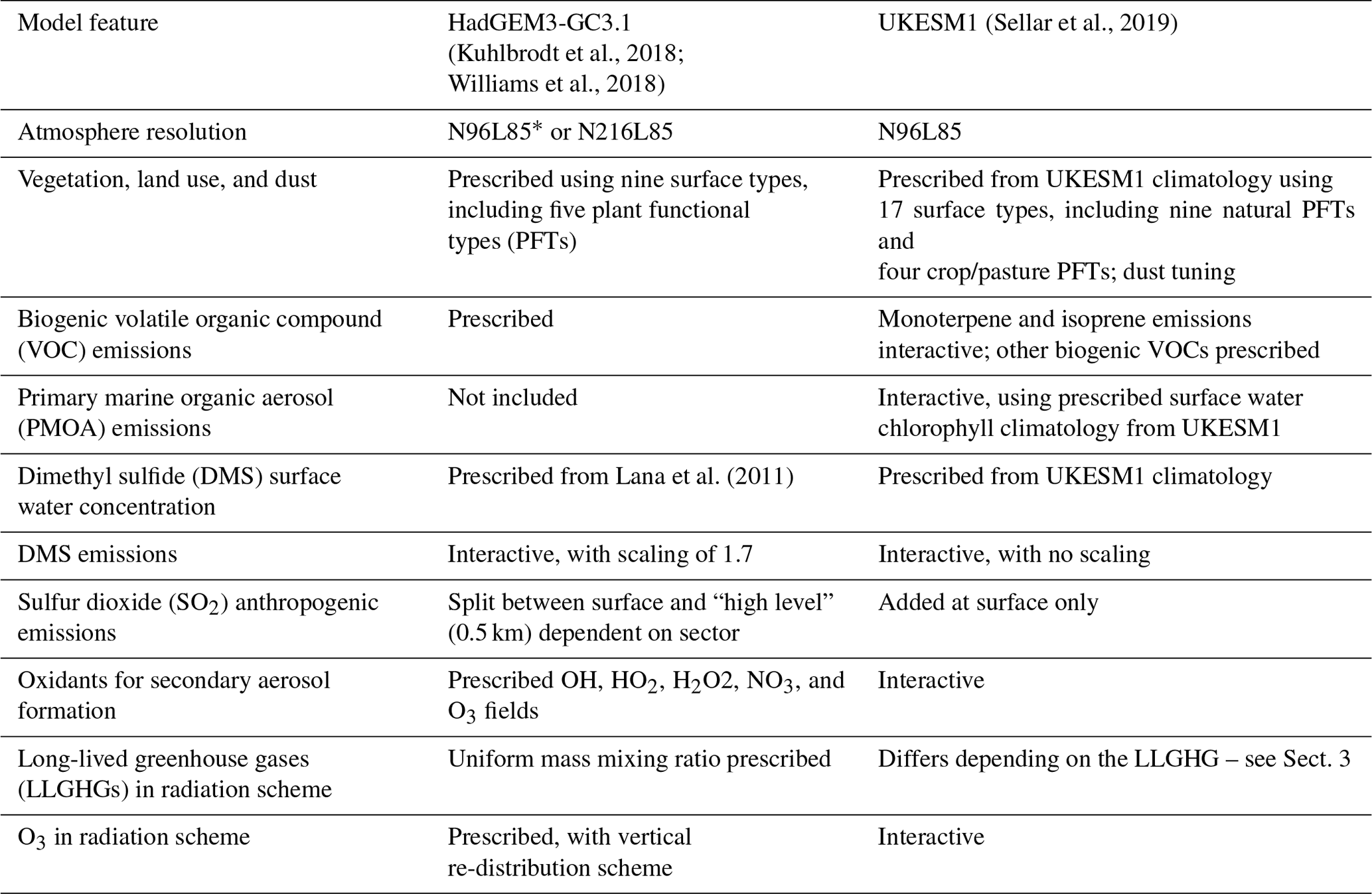
^* Atmosphere resolution of HadGEM3-GC3.1 used in the Tier 1 RFMIP simulations (Andrews et al., 2019).