the Creative Commons Attribution 4.0 License.
the Creative Commons Attribution 4.0 License.
 | 11 Aug 2021
Spatiotemporal changes in aerosol properties by hygroscopic growth and impacts on radiative forcing and heating rates during DISCOVER-AQ 2011
David N. Whiteman
Igor Veselovskii
Richard Ferrare
Gloria Titos
María José Granados-Muñoz
Guadalupe Sánchez-Hernández
Francisco Navas-Guzmán
This work focuses on the characterization of vertically resolved aerosol hygroscopicity properties and their direct radiative effects through a unique combination of ground-based and airborne remote sensing measurements during the Column and Vertically Resolved Observations Relevant to Air Quality (DISCOVER-AQ) 2011 field campaign in the Baltimore–Washington DC metropolitan area. To that end, we combined aerosol measurements from a multiwavelength Raman lidar located at NASA Goddard Space Flight Center and the airborne NASA Langley High Spectral Resolution Lidar-1 (HSRL-1) lidar system. In situ measurements aboard the P-3B airplane and ground-based Aerosol Robotic Network – Distributed Regional Aerosol Gridded Observational Network (AERONET-DRAGON) served to validate and complement quantifications of aerosol hygroscopicity from lidar measurements and also to extend the study both temporally and spatially. The focus here is on 22 and 29 July 2011, which were very humid days and characterized by a stable atmosphere and increasing relative humidity with height in the planetary boundary layer (PBL). Combined lidar and radiosonde (temperature and water vapor mixing ratio) measurements allowed the retrieval of the Hänel hygroscopic growth factor which agreed with that obtained from airborne in situ measurements and also explained the significant increase of extinction and backscattering with height. Airborne measurements also confirmed aerosol hygroscopicity throughout the entire day in the PBL and identified sulfates and water-soluble organic carbon as the main species of aerosol particles. The combined Raman and HSRL-1 measurements permitted the inversion for aerosol microphysical properties revealing an increase of particle radius with altitude consistent with hygroscopic growth. Aerosol hygroscopicity pattern served as a possible explanation of aerosol optical depth increases during the day, particularly for fine-mode particles. Lidar measurements were used as input to the libRadtran radiative transfer code to obtain vertically resolved aerosol radiative effects and heating rates under dry and humid conditions, and the results reveal that aerosol hygroscopicity is responsible for larger cooling effects in the shortwave range (7–10 W m−2 depending on aerosol load) near the ground, while heating rates produced a warming of 0.12 K d−1 near the top of PBL where aerosol hygroscopic growth was highest.
- Article
(15728 KB) - Full-text XML
- BibTeX
- EndNote


Improving our knowledge of atmospheric aerosols is essential to better understanding their role in climate projections because of the uncertainties associated with how atmospheric aerosol particles scatter and absorb solar radiation (direct effect) and how they act as cloud condensation nuclei which affect cloud formation and evolution (Lohman and Feichter, 2005; Haywood and Schulz, 2007). In spite of the advances in understanding aerosol radiative effects, the most recent Intergovernmental Panel on Climate Change (IPCC) model estimates call for improved understanding of the aerosol indirect effect (Boucher et al., 2013). Although satellite missions and ground-based networks have provided an unprecedented advance in the global knowledge of aerosol optical and microphysical properties, there are still many gaps in the understanding of aerosol changes due to their interaction with water vapor in the atmosphere (Boucher, 2015; Seinfield and Pandis, 2016). Field campaigns are ideal for advancing our understanding of these changes in aerosol properties with water vapor and in how these changes eventually impact direct radiative forcing and cloud formation (Gysel et al., 2007). Ideally, these field campaigns include many remote sensing and in situ instruments because each instrument provides unique information.
Aerosol hygroscopic growth implies changes in aerosol optical and microphysical properties with changing relative humidity (e.g., Titos et al., 2016). Because of the ubiquitous nature of water vapor in Earth's atmosphere, studying aerosol hygroscopicity is essential for improving our understanding of the role of aerosols in climate (Haywood and Shine, 1995; Pilinis et al., 1995). Hydrophilic particles absorb water vapor and thus increase their size and become more efficient scatterers (e.g., Zieger et al., 2013). The magnitude of water vapor uptake by an aerosol particle depends directly on their size and chemical composition (Zieger et al., 2013). Hydrophobic aerosols (e.g., mineral particles) show very little variation of their properties with relative humidity (Kotchenruther and Hobbs, 1998; Gassó et al., 2000; Fierz-Schmidhauser et al., 2010a; Titos et al., 2014), while hydrophilic particles (e.g., sulfates, water-soluble organic carbonaceous particles) are very sensitive to the uptake of water vapor (e.g., Zieger et al., 2013). Many studies have also demonstrated that hygroscopic growth can accelerate the formation and evolution of haze pollution (e.g., Yang et al., 2015; Chen et al., 2019). Model simulations can be used to evaluate changes in final aerosol direct radiative forcing based on pre-determined models of aerosol hygroscopic growth (e.g., Bian et al., 2009). Actually, Burgos et al. (2019) illustrated that Earth system global models showed a large diversity in predicting the impact of enhanced relative humidity on aerosol scattering properties, being mainly driven by differences in hygroscopicity parameterizations within the models and model chemistry.
Ground-based in situ measurements with tandem nephelometers have been widely used to investigate the effect of hygroscopic growth on aerosol scattering properties (e.g., Fierz-Schmidhauser et al., 2010b; Burgos et al., 2019). However, these in situ measurements are representative only of a few meters above the ground. Tandem nephelometers have also been used aboard aircraft (e.g., Sheridan et al., 2002; Shinozuka et al., 2007) during field campaigns to provide vertically resolved information on aerosol hygroscopic properties, but such measurements are sparse. Thus, to improve the characterization of aerosol hygroscopicity, the combined use of remote sensing techniques and other meteorological measurements is called for. The use of ground-based Sun photometers from the Aerosol Robotic Network (AERONET) network (e.g., Holben et al., 1998) can provide general insight into aerosol hygroscopicity by analyzing changes in aerosol size distribution with water vapor content (e.g., Schafer et al., 2008), but these characterizations are representative of the column-integrated aerosol. The combination of lidar with other meteorological measurements is ideal for answering questions about the vertically resolved aerosol hygroscopicity but requires the assumption of well-mixed conditions to isolate aerosol hygroscopicity from other aerosol processes (Wulfmeyer and Feingold, 2000; Feingold and Morley, 2003). This technique has been widely used for backscattering lidars (e.g., Granados-Muñoz et al., 2015; Haeffelin et al., 2016; Lv et al., 2017; Zhao et al., 2017; Fernández et al., 2018; Bedoya-Velasquez et al., 2018, 2019; Navas-Guzmán et al., 2019; Dowson et al., 2020). However, to obtain information on how aerosol hygroscopicity affects the aerosol microphysical properties with altitude requires the application of inversion algorithms that use at least measurements of aerosol extinction (α) at two wavelengths (typically 355 and 532 nm) and of backscattering (β) at three wavelengths (typically at 355, 532 and 1064 nm). This approach is generally known as the lidar 3β+2α technique and uses inversion with regularization (e.g., Müller et al., 1999; Veselovskii et al., 2002). Because well-mixed conditions in the boundary layer typically occur during daytime, retrievals of aerosol microphysical properties of aerosol hygroscopic growth during daytime using Raman lidar are limited due to the difficulty of obtaining independent daytime extinction measurements and the need for very optimized lidar systems (e.g., Whiteman et al., 2006a, b; Dawson et al., 2020). Thus, extrapolations have been done using the closest nighttime measurements (e.g., Veselovskii et al., 2009). However, thanks to the latest technological developments, independent vertical profiles during daytime of aerosol extinction and backscattering can be measured using High Spectral Resolution Lidar-1 (HSRL-1) (e.g., Hair et al., 2009; Burton et al., 2018) and/or Raman lidar with high-power lasers (e.g., Whiteman et al., 2006, 2007) with the use of rotational Raman narrowband filters expanding the use of Raman lidars for daytime measurements (e.g., Ortiz-Amezcua et al., 2019).
Determining aerosol direct radiative effects and heating rates has been challenging in the last decades because their computation requires considerable knowledge of aerosol optical and microphysical properties in order to constrain radiative transfer models (e.g., Ramanathan et al., 2001; Forster et al., 2007; Myhre et al., 2013). To that end, several recent field campaigns have been performed to characterize aerosol radiative forcing (e.g., Ramanathan et al., 2007; Mallet et al., 2016). Other studies focused on the characterization of dust radiative effects and heating rates from particular sites (Huan et al., 2009; di Sarra et al., 2011; Perrone et al., 2012; Meloni et al., 2015; Bhawar et al., 2016), and even differentiating between aerosol fine and coarse modes to characterize shortwave and longwave radiative effects (Sicard et al., 2014). All previous studies remarked that to minimize the errors in the computations of aerosol radiative effects it is critical to know the aerosol vertical distribution (Haywood and Ramaswany, 1998; Guan et al., 2010). In this sense, independent lidar measurements of extinction and backscattering provided by Raman or HSRL systems can minimize errors in radiative forcing computations (e.g., Lolli et al., 2018). To improve the use of lidar data for quantifying vertically resolved aerosol radiative forcing, it is necessary to understand how aerosol interacts with other gases in the atmosphere such as water vapor (e.g., Smith et al., 2020; Thorsen et al., 2020) and thus how aerosol hygroscopic growth affects radiative forcing (Rastak et al., 2014).
The Deriving Information on Surface conditions from the Column and Vertically Resolved Observations Relevant to Air Quality (DISCOVER-AQ) field campaign conducted in July 2011 in the Baltimore–Washington DC metropolitan area was a NASA-sponsored field campaign designed to investigate air quality (Crawford and Pickering, 2011) using both airborne and ground-based instrumentation. The airborne assets used in DISCOVER-AQ were the NASA P-3B equipped with a variety of in situ measurements for aerosol and gas characterization and the Beechcraft King Air UC-12, where the HSRL-1 (Hair et al., 2009) was installed. Moreover, a unique ground-based set of instrumentation including the multiwavelength Raman lidar system at NASA Goddard Space Flight Center (e.g., Veselovskii et al., 2013, 2015a) was deployed. The combination of airborne and ground-based lidar instruments during DISCOVER-AQ has previously been demonstrated as a useful approach to get accurate 3β+2α measurements used in the inversion by regularization to obtain aerosol microphysical properties (e.g., Sawamura et al., 2014). Moreover, the AERONET-DRAGON (Distributed Regional Aerosol Gridded Observational Network; Holben et al., 2018) Sun photometer network deployment permitted regional aerosol optical depth (AOD) to be characterized at high spatial resolution. AERONET-DRAGON measurements during DISCOVER-AQ 2011 have been used to identify the enhancement of AOD in the presence of cumulus clouds (Eck et al., 2014) but not on how hygroscopic growth can affect the enhancement of AOD over an entire region. Other studies using P-3B data from DISCOVER-AQ 2011 served to identify sulfate and other inorganic compounds as the main aerosol species present during the campaign (e.g., Beyersdorf et al., 2016) and their possible impact on aerosol hygroscopicity (e.g., Ziemba et al., 2012; Crumeyrolle et al., 2014; Chu et al., 2015). However, there were no closure studies performed on the impact of aerosol hygroscopicity on vertical profiles of aerosol optical and microphysical properties and their impact on radiative forcing.
The objective of this work is to study how hygroscopic growth affects vertically resolved aerosol optical and microphysical properties and then to understand how aerosol hygroscopicity affects aerosol loading and radiative forcing. To that end, a unique dataset of measurements acquired during DISCOVER-AQ 2011 was used with special emphasis on the combination of different multiwavelength lidar systems. Particularly the combination of measurements from the NASA Goddard Space Flight Center (GSFC) Raman lidar and the airborne HSRL-1 provided the 3β+2α measurements during daytime. Extensive radiosonde measurements were conducted at the Howard University Beltsville Campus in Beltsville, Maryland, to support DISCOVER-AQ 2011 measurements.
This paper is structured as follows: Sect. 2 describes the methodology used. Section 3 is devoted to the main results, while conclusions are given in Sect. 4.
2.1 DISCOVER-AQ 2011 I: airborne instrumentation
DISCOVER-AQ was a multi-year and multi-city NASA mission designed to study air quality in urban environments. Here we focus only on the component of the experiment that was performed in the Baltimore–Washington DC urban region during July 2011 covering a study area approximately from 38.75 to 39.75∘ N and from 77.75 to 75.25∘ W.
The NASA P-3B airplane was equipped with a variety of in situ instruments to study aerosol and gas-phase particles in the atmosphere. The P-3B flew 14 missions over 29 d in July 2011 including spirals (both up and down) at different reference sites with at least three spirals per site. Figure 1a shows an example of the flight track and spirals performed by the P-3B on 29 July. The NASA Langley Aerosol Group Experiment (LARGE – https://science.larc.nasa.gov/large/, last access: 23 June 2021) deployed several in situ instruments for aerosol characterization: (1) an isokinetic inlet capable of collecting and transmitting particles with diameter smaller than 0.4 µm (McNaughton et al., 2007), (2) an integrating nephelometer (TSI, Inc. model 3563) measuring aerosol scattering coefficients at 450, 550 and 700 nm, (3) a particle soot absorption photometer (PSAP, Radiance Research) measuring aerosol absorption coefficients at 470, 532 and 660 nm. Combining integrating nephelometer and PSAP measurements, the aerosol extinction coefficient and single scattering albedo (ratio of the scattering to the extinction coefficients) are computed using the Ångström exponent to obtain scattering coefficient at 532 nm. But all of these measurements are acquired under dry conditions (the sampled air is adjusted to 20 % relative humidity; Beyersdorf et al., 2016), and to study the effect of enhanced relative humidity in the scattering coefficients (and adjust the measured value to real atmospheric conditions) another integrating nephelometer is used. This second nephelometer is equipped with a humidification system capable of adjusting relative humidity inside the instrument to 80 %. The tandem of nephelometers permits the characterization of the aerosol scattering enhancement factor f(RH) defined as the ratio of aerosol scattering at a certain relative humidity (RH) to the corresponding dry (or reference) scattering coefficient (e.g., Titos et al., 2016). The enhancement factor can be parameterized as a function of RH using the Hänel equation, expressed as (Hänel, 1976)
where γ is the hygroscopic growth parameter that quantifies the hygroscopic scattering enhancement. From the tandem nephelometer measurements and the ambient RH (RHamb), it is possible to determine the scattering coefficient at ambient conditions (σamb) as (e.g., Beyersdorf et al., 2016)
The dependence of absorption with relative humidity is highly uncertain (e.g., Brem et al., 2012). Nevertheless, for the aerosol types present during DISCOVER-AQ 2011, aerosol absorption was very low, thus contributing less than 4 % to aerosol extinction with minimum influence on extinction and single scattering albedo (e.g., Ziemba et al., 2013).
The aerosol size distribution was measured by several instruments with each one covering a certain diameter range: the aerosol particle sizer (APS, TSI) for the 0.5–20 µm range, the scanning mobility particle sizer spectrometer (SMPS-TSI) for the 10–300 nm range, the ultra-high sensitivity aerosol spectrometer (UHSAS, Droplet Measurement Technologies) for the 60–950 nm range and the Particle Measure System model LAS-X (LAS, Particle Measuring System, Inc.,) for the range 0.12–7.5 µm range. All of these instruments provided aerosol size distribution under dry conditions which can differ from that in the real atmosphere. On the other hand, water-soluble organic and inorganic species were obtained from a pair of particle-into-liquid samplers (PILSs, Brechtel Manufacturing, Inc.; Weber et al., 2001). The liquid flow from the second PILS was collected in vials with 3–5 min temporal resolution for offline ion chromatographic analysis of water-soluble organic carbon, chloride, nitrate, nitrite, sulfate, sodium, ammonium, potassium, magnesium and calcium mass concentrations (see Beyersdorf et al., 2016 for details).
The NASA Beechcraft King Air UC-12 airplane operated a compact HSRL to obtain vertical profiles of the atmosphere. The HSRL system used spectral sampling of the lidar returned signal to discriminate the aerosol and molecular components, thus permitting independent measurements of aerosol backscattering and extinction coefficients. During DISCOVER-AQ 2011, the HSRL-1 system was capable of obtaining extinction, backscattering and depolarization profiles at 532 nm, and backscattering and depolarization profiles at 1064 nm (Hair et al., 2008; Rodgers et al., 2009). In total, 13 d of flights with two flights per day were performed at a nearly constant altitude of ∼ 8 km. Backscattering and depolarization profiles have a vertical resolution of 30 m and 10 s (∼ 1 km) horizontal resolution, while aerosol extinction profiles have 300 m vertical and 60 s (∼ 6 km) horizontal resolution. Figure 1b shows the flight track followed by the NASA UC-12 airplane on 29 July 2011. Data from both airplanes used in this study are freely available at the NASA Airborne Science Data for Atmospheric Composition (https://www-air.larc.nasa.gov/cgi-bin/ArcView/discover-aq.dc-2011, last access: 7 September 2018).
2.2 DISCOVER-AQ 2011 II: ground-based instrumentation
DISCOVER-AQ 2011 also included a large set of ground-based measurements that complemented those obtained from the aircraft. Among the most relevant to our work are those provided by the AERONET-DRAGON network (Holben et al., 2018) that provided wide spatial and temporal Sun–sky radiometry measurements of spectral AODs and of inversion products such as aerosol size distribution, refractive indices and single scattering albedo (e.g., Dubovik and King, 2000; Dubovik et al., 2000, 2006). For the DISCOVER-AQ campaign, DRAGON consisted of 43 AERONET sites in the Baltimore–Washington DC region covering a region approximately 125 km long and 40 km wide, following the I-95 corridor from Washington Beltway north to the Maryland–Delaware state line and encompassing both the Baltimore and Washington DC suburbs agricultural areas and the Chesapeake Valley. Figure 1c illustrates the spatial distribution of all stations during this field campaign. For the analysis here, we used AERONET Level 2.0 version 3 data (Giles et al., 2019).
The multiwavelength Mie–Raman lidar deployed at NASA GSFC (38.99∘ N, 76.84∘ W; 87 m a.s.l.) was unique in providing vertically resolved aerosol properties. The system consisted of a high-power Nd:YAG (neodymium-doped yttrium aluminum garnet – Nd : Y3Al5O12) laser operating at a 50 Hz repetition rate with output powers of approximately 15, 7 and 12 W at 355, 532 and 1064 nm wavelengths. The detector system consisted of a 40 cm aperture Schmidt–Cassegrain telescope operated vertically with a 0.5 mrad field of view (FOV). The system used interference filters to measure backscattered light at the three laser emission wavelengths plus two additional filters for detecting nitrogen Raman signals at 387 and 607 nm. Complete lidar overlap occurred at an altitude of approximately 1000 m a.g.l. For each profile, 6000 laser pulses were accumulated, which implied a temporal resolution of 2 min. The high-power output of the laser permitted Raman measurements only at 387 nm during daytime, while for nighttime both Raman measurements were possible. Details of this system can be found in Veselovskii et al. (2013, 2015a, b). In addition, during the field campaign, radiosondes were launched approximately every 4 h at the Howard University Beltsville Campus (HUBC). HUBC is approximately 8 km distance from GSFC, and radiosonde measurements from HUBC were used to complement Raman lidar measurements by providing vertical profiles of temperature and relative humidity.
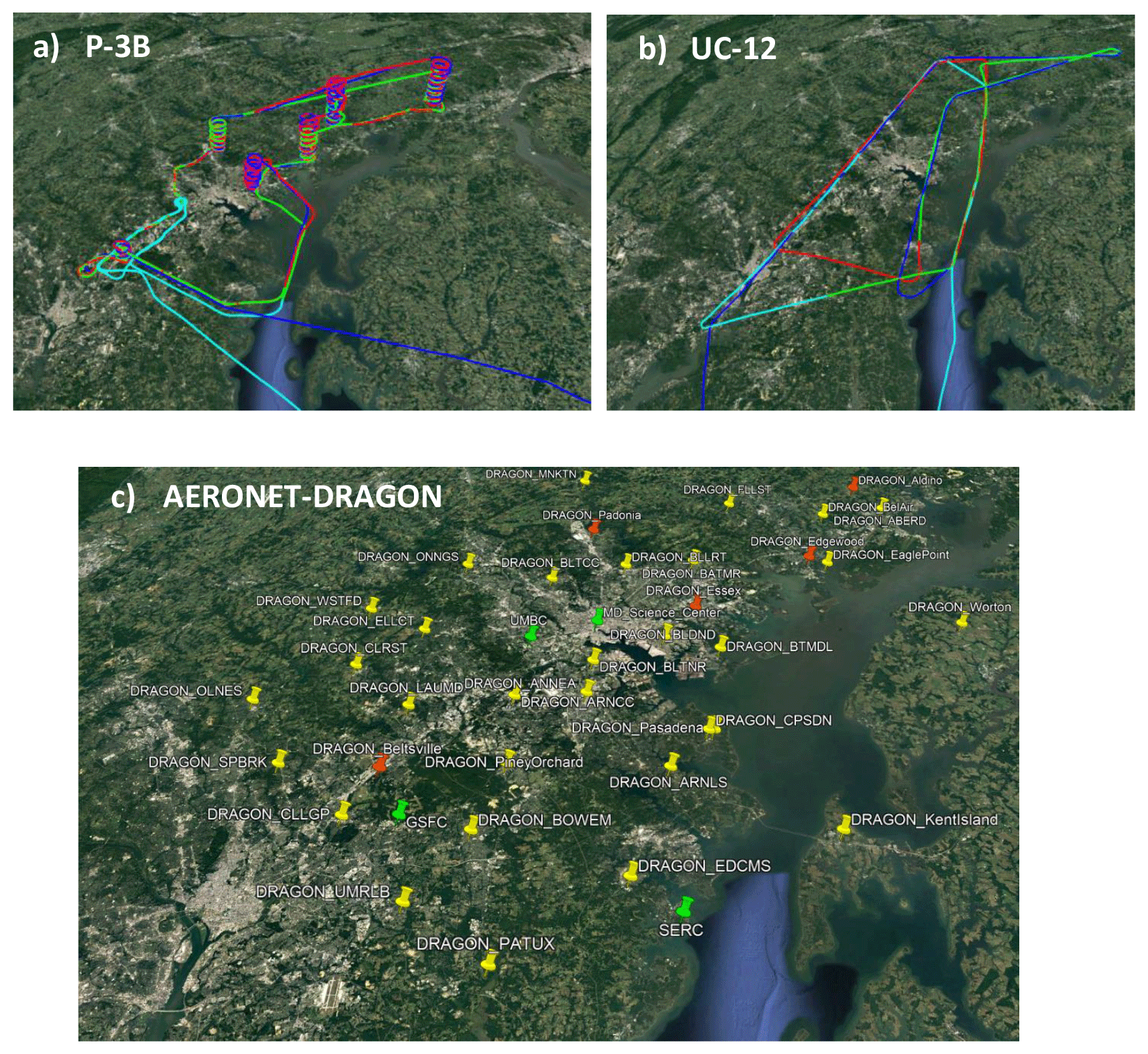
Figure 1For 29 July 2011: (a) flight track for P-3B airplane, (b) flight track for the UC-12 airplane and (c) AERONET-DRAGON stations. The region is the Baltimore–Washington DC area, covering approximately from 38.75 to 39.75∘ N and from 77.75 to 75.25∘ W. Maps attribution are Google Landsat/Copernicus Data SIO, NOAA, US Navy, GEBCO. Data LDEO-Columbia, NSF, NOAA.
2.3 Retrieval of vertically resolved aerosol microphysical properties
When HSRL-1 flew over GSFC, the combination of backscattering at 355 and 1064 nm, and extinction at 355 nm from the ground-based Mie–Raman system with backscattering and extinction at 532 nm from the HSRL-1 system provided sufficient measurements to perform 3β+2α inversions by solving the ill-posed problem using regularization (e.g., Müller et al., 1999; Veselovskii et al., 2002; Sawamura et al., 2014). The overlap of these two lidar systems permitted us to obtain the 3β+2α with no a priori assumptions of lidar ratio. But the inversion is underdetermined because of the larger number of retrieved parameters than input optical data (e.g., Veselovskii et al., 2005; Burton et al., 2016). Therefore, we use an averaging procedure that consists of selecting many solutions in the vicinity of the minimum discrepancy (e.g., Veselovskii et al., 2002). Moreover, constraints in the inversion need to be applied to avoid undesirable solutions (e.g., Whiteman et al., 2018) and the inversion approach uses case-dependent optimized constraints that limit the ranges of allowed radius and refractive indexes (Pérez-Ramírez et al., 2019, 2020). HSRL-1 coincident data with Mie–Raman measurements are obtained by averaging a maximum of 5 min measurements to guarantee co-location, while Mie–Raman data are averaged every 15 min. The averaging of lidar data is performed to obtain better signal-to-noise ratios, which is particularly important for extinction computations which are the parameters to which the inversion by regularization is most sensitive (Pérez-Ramírez et al., 2013).
2.4 Computations of aerosol radiative forcing and heating rates
The aerosol radiative effect (ARE) is defined as the perturbation in the solar flux caused by the presence of aerosols in relation to a clean (clear-sky, non-aerosol) atmosphere. Thus, aerosol radiative effect within a layer “z” that is computed as the difference between two sets of radiative fluxes:
where F↓(z)A and F↑(z)A are the downward and upward fluxes at level z in the presence of aerosols, while F↓(z)0 and F↑(z)0 are the downward and upward fluxes with no aerosols present. The absorption of solar radiation due to aerosols is quantified through the heating rates (HRs) that can be defined as (Liou, 2002)
where is the heating rate at an altitude z, Cp is the specific heat of the air at constant pressure, ρ is the air density and ΔF(z) is the net flux density divergence or ARE(z) for a given layer of thickness Δz.
Our computations of AREs and HRs were performed with the libRadtran radiative transfer model version 2.0.2 (Emde et al., 2016). In the computations with libRadtran, gas parameterizations from Santa Barbara DISORT atmospheric radiative transfer software (SBDART; Ricchiazzi et al., 1998) and the amounts given for the US standard atmosphere were used. Surface albedos were obtained from the AERONET-based surface reflectance validation network (ASRVN; Wang et al., 2011). The large set of data obtained during DISCOVER-AQ allowed the code to be run using real measurements, in particular, water vapor and temperature profiles from radiosondes launched at HUBC, aerosol single scattering albedo and asymmetry factor obtained from the P-3B aircraft (measured by in situ instrumentation) and AERONET (inversions of Sun and sky radiances), and most importantly aerosol extinction and backscattering profiles obtained from lidar measurements. Particularly, we used the set of 3β+2α as input to the radiative transfer model. Outputs from the computations are vertical profiles of ARE and the aerosol HR at 355, 532 and 1064 nm, and also integrated values in the shortwave range between 0.280 and 3 µm. The use of 3β+2α profiles minimizes the errors in ARE and HR associated with the vertical distribution of aerosols (e.g., Haywood and Ramaswany, 1998; Guan et al., 2010; Gómez-Amo et al., 2014; Thorsen et al., 2020), and because we use independent measurements by Raman and HSRL systems, this approach should reduce errors associated with the lidar methodology (Lolli et al., 2018).
3.1 Impacts of systematic and random uncertainties in determining aerosol hygroscopicity parameter from lidar-derived parameters
The approach to identify the conditions for studying aerosol hygroscopicity in the atmospheric aerosol profile with lidar systems consists of identifying well-mixed layers that guarantee the same type of aerosol and constant water vapor mixing ratio with altitude (e.g., Veselovskii et al., 2009). Under these conditions, enhancement of aerosol backscattering or extinction with relative humidity can be associated directly with water vapor uptake by aerosol particles (e.g., Ferrare et al., 1998; Wulfmeyer and Feingold, 2000). In such circumstances, an increase of relative humidity with altitude is typically observed, and the Hanël equation, including lidar backscattering coefficients, is given as
where RHref and βref are the relative humidity and aerosol backscattering coefficients at the lowest altitude of lidar measurements, respectively. Taking logarithms of both sides of Eq. (5) yields
And now a linear regression of the measurements of β(z) and RH(z) at altitudes exhibiting aerosol hygroscopic growth provides the hygroscopic growth parameter “γ” as the slope of the best-fit equation.
The impact of systematic and random uncertainties in relative humidity on the computation of the hygroscopic growth parameter “γ” is studied here to determine the uncertainties in γ that are obtained from lidar measurements and to understand better how γ obtained from lidar measurements compares with values obtained from other measurements. First, the effects of random uncertainties in estimations of γ are studied through simulations where uncertainties in relative humidity was generated from a Gaussian distribution centered at zero with width equal to the random uncertainty desired (1 %, 2 %, 3 %, 5 %, 7 %, 8 %, 10 %, 20 %, 25 % and 30 %). We note that random uncertainties in relative humidity with radiosondes are % (e.g., Milosevich et al., 2009), while those obtained by lidar can be as large as ±30 % or more depending on lidar measurement statistics (e.g., Whiteman et al., 2007). The procedure for the simulations consists of using Eq. (5) with γ equal to 0.4, 0.6, 0.8, 1.0 and 1.2 to calculate the value of f(RH) for a set of relative humidity ranging from 20 to 100 % and with no errors. Later, random uncertainty is added to relative humidities, and the new set of data is used with f(RH) in Eq. (6) to compute the new value of γ′. Figure 2a shows the relative difference in hygroscopicity parameter versus random uncertainties in relative humidity. The mean differences are shown with errors bars indicating the standard deviations of the spread in the results. Figure 2a clearly indicates that relative differences in γ increase in absolute value until reaching approximately constant values of −20 % for random uncertainties larger than 10 %. Actually, for random uncertainties below 5 %, typical of radiosondes, uncertainties in γ are below −15 %. We note that in all computations, random uncertainties were positive. Including negative random uncertainties provided a symmetric graph (not shown for simplicity)
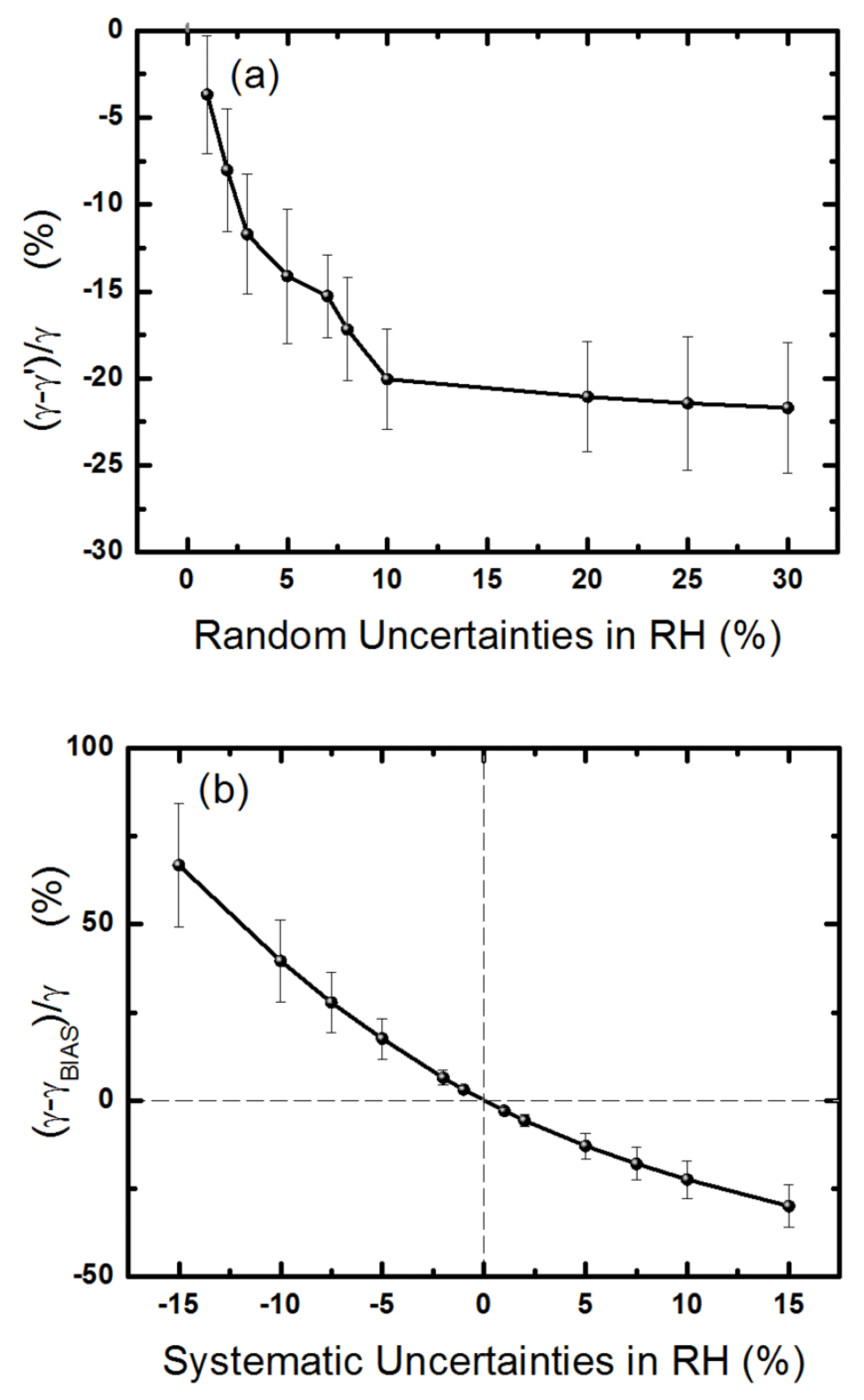
Figure 2Sensitivity analyses of the hygroscopic growth parameter “γ” as function of (a) random errors in the relative humidity and (b) systematic errors in relative humidity.
To evaluate the effects of systematic uncertainties in relative humidity on the calculation of γ, we again performed simulations but applied a fixed bias over the entire range of relative humidity. These biases are associated with systematic uncertainties which vary from −15 % to +15 % in the simulation. With relative humidity affected by bias, a new hygroscopicity parameter, γBIAS, is computed and serves to evaluate the relative differences . Figure 2b shows mean values and standard deviations of the relative differences. Figure 2b clearly shows a decrease in relative differences from ∼ 65 % for biases of −15 % to −30 % for biases of ∼ 15 %. For biases within ±5 %, which is what radiosondes can possess due to dry biases (Milosevich et al., 2009), the uncertainties in γ are in the range ±15 %. Based on all these results, we can conclude that the assessment of gamma is considerably more sensitive to systematic uncertainties in RH than random uncertainties.
3.2 Characterization and validation of aerosol hygroscopicity computed with lidar measurements
During DISCOVER-AQ, typical summertime mid-Atlantic conditions of hot and humid days were present. This weather, coupled with local emissions and transport of anthropogenic aerosol, produced ideal conditions for studying aerosol hygroscopicity. Because of the limited availability of Mie–Raman ground-based measurements during DISCOVER-AQ 2011, only two particular days were identified for studying aerosol hygroscopicity with lidar measurements.
The first day was 29 July 2011, which offered a 10 h record of daytime ground-based Mie–Raman measurements. Backward trajectories computed by the Hybrid Single-Particle Lagrangian Integrated Trajectory (HYSPLIT) model (Stein et al., 2015) revealed very stable atmospheric conditions on this day with air masses predominantly coming from the Ohio River Valley (graphs not shown for simplicity). The temporal evolution of atmospheric profiles of water vapor mixing ratio (Fig. 3a) revealed a well-mixed lower atmosphere at 20:00 UTC with a constant water vapor mixing ratio of ∼ 12.0 g kg−1 from the ground up to ∼ 2.2 km (Fig. 3b). In this layer, relative humidity increased from ∼ 33 % at the surface to ∼ 75 % at 2.2 km, as shown in Fig. 3b. During the rest of the days, well-mixed conditions were not present, as revealed by the variability of water vapor mixing ratio with height in the first kilometers above the ground.
The other case study occurred on 22 July 2011, although for this case the Mie–Raman lidar measurements were sparse extending from 18:00 to 19:00 UTC approximately. According to HYSPLIT, air masses again had their origin in the Ohio River Valley. On this day at 18:15 UTC, water vapor mixing ratio profiles from HUBC radiosonde measurements (Fig. 3c) revealed two very stable atmospheric layers: the first from the ground up to approximately 1.8 km, with a constant water vapor mixing ratio of ∼ 15.5 g kg−1, and the second from 3 to 4.5 km with a much lower water vapor mixing ratio of ∼ 3.5 g kg−1. Both layers were characterized by an increase of relative humidity from the bottom to the top of the layers (Fig. 3d), although only the first layer covered a range of relative humidity large enough to study aerosol hygroscopic growth (from 40 % to 80 % approximately). These patterns of water vapor mixing ratio and relative humidity variation with height seem to start early, as suggested by the data at 13:57 UTC. Stable conditions are also observed at 03:51 UTC but not for the rest of the hours when large variability of relative humidity is observed near the surface.

Figure 3Water vapor mixing ratio and relative humidity profiles obtained from radiosondes launched at HUBC on (a–b) 29 July 2011 and (c–d) 22 July 2011.
Figure 4 shows temporal evolution of α(355) from multiwavelength Raman lidar measurements performed at GSFC on 29 July 2011 using the Klett method (Klett, 1985) with an extinction-to-backscattering ratio, otherwise known as the lidar ratio (LR), of 85, which was computed from correlative AERONET inversions. The use of fixed lidar ratio and the hypotheses in its computation induces errors in backscattering retrievals, but the Klett method is used here for the visualization of data with high temporal resolution (1 min). In Fig. 4, times when HSRL-1 flew over GSFC are indicated with white lines, while dotted lines indicate when the P-3B airplanes performed spirals over the HUBC. Times of coincident radiosondes are shown with dashed white lines.
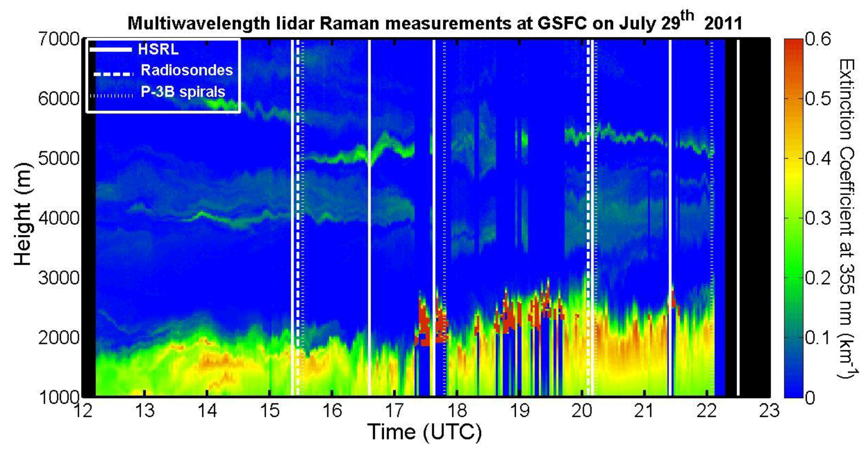
Figure 4Time evolution of aerosol extinction coefficient at 355 nm from GSFC Raman lidar measurements on 29 July 2011. Extinction data are computed using the Klett method with a lidar ratio of 85 sr. Vertical resolution is 7.5 m. Also noted in the plot are overpasses by the HSRL-1 system and correlative spirals by the P-3B airplane with in situ instrumentation close to GSFC-HUBC region. Times when radiosondes were launched are also illustrated.
Figure 4 indicates that most aerosols are within the planetary boundary layer (PBL) with sporadic and thin decoupled layers between 4–5 km that are associated with transport of biomass burning from fires active in the western US (https://firms.modaps.eosdis.nasa.gov/, last access: 22 March 2021). But the most important feature to note is the evolution of aerosols within the PBL throughout the measurement period. Early in the morning, decoupled aerosol layers are observed (note that local time is UTC−4). At approximately 16:00 UTC, it is observed that as the PBL height increases intense red areas corresponding to convective clouds formed at the top of the boundary layer. After approximately 19:40 UTC, there were clear skies, and the most remarkable feature is the increase of aerosol extinction with altitude over approximately 2.5 h, and the combination of Mie–Raman with HSRL-1 measurements serves to get 3β+2α measurements and study the possible influence of aerosol hygroscopicity based on lidar measurements.
Figure 5 shows lidar-derived parameters for two selected case studies when 3β+2α measurements were possible for studying aerosol hygroscopicity. The two selected cases are on 29 July at 20:00 UTC (Fig. 5a–b) and 22 July at 18:35 UTC (Fig. 5c–d). Data are shown for the region above 1 km a.g.l. where Raman lidar measurements had complete overlap. Specifically, Fig. 5 also shows correlative measurements of aerosol backscattering at 355, 532 and 1064 nm between ground-based Mie–Raman lidar and airborne HSRL-1. For aerosol extinction backscattering coefficients at 532 nm, the reference measurements are from HSRL-1 because it obtains independent extinction and backscattering measurements at this wavelength, while at 1064 nm we present just a comparison because both lidar systems are only capable of obtaining backscattering measurements at this wavelength. On the other hand, the Mie–Raman system provided independent aerosol extinction and backscattering coefficients at 355 nm using the Raman measurements at 387 nm and therefore is used as a reference, while for 532 and 1064 nm the Klett method is used with LRs of 65 and 30 on 29 July and 55 and 40 on 22 July for 532 and 1064 nm, respectively. For both days, Fig. 5 indicates that both instruments reveal very similar values and vertical patterns in backscattering and extinction, which illustrates the consistency of the measurements and lends confidence to their use as a set of 3β+2α measurements.
Figure 5a–b show that at 20:00 UTC on 29 July both backscattering and extinction increase with altitude in the planetary boundary layer. The constant water vapor mixing ratio and the increase of relative humidity with altitude at 20:19 UTC (Fig. 3a–b) make this set of 3β+2α measurements ideal for studying aerosol hygroscopicity. On 22 July at 18:35 UTC, an increase of extinction and backscattering with height is observed again, and the closest radiosonde was at 18:15 UTC (Fig. 3c–d), indicating well-mixed conditions that were therefore good for studying aerosol hygroscopic growth during the day. Unfortunately, there were only ∼ 2 h of multiwavelength ground-based Raman lidar on 22 July, and measurements on this day will serve to complement the large set of measurements for 29 July.
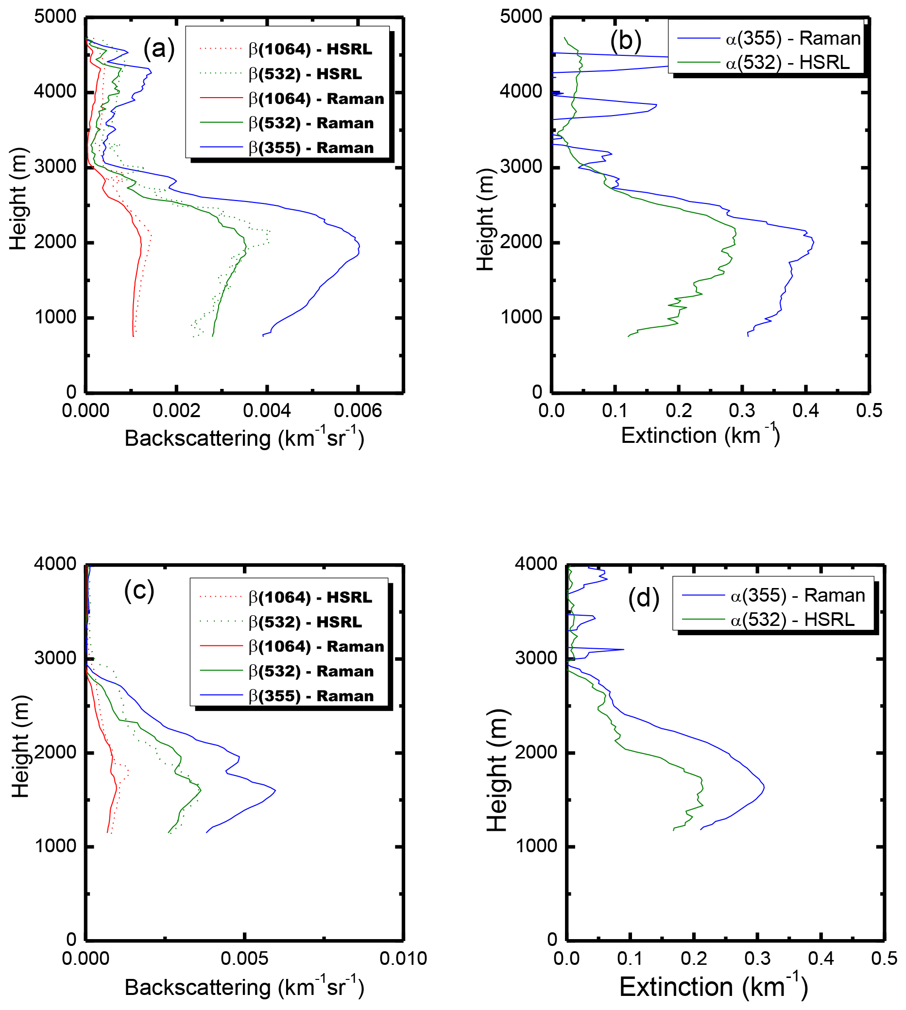
Figure 5Vertical profiles of backscattering (β) and extinction (α) measurements obtained by ground-based Raman lidar and airborne HSRL-1 at NASA Goddard Space Flight Center on (a–b) 29 July 2011 at 20:00 UTC and (c–d) 22 July 2011 at 18:35 UTC. The ground-based Mie–Raman measurements provided independent measurements of backscattering and extinction coefficients at 355 nm, while the airborne HSRL-1 system provided those for 532 nm. For 1064 nm, both instruments provided only backscattering measurements.
Table 1Results of the linear fits of log(f(RH)) versus log((1-RH) (1 RHref)). The computation of f(RH)∗ was done using Eq. (5) with RH = 80 % and RHref=20 % for intercomparisons with a tandem of nephelometers.
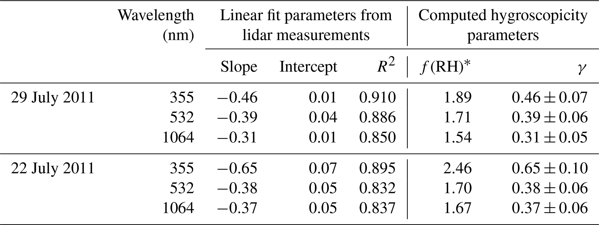
Figure 6 shows f(RH) – computed as – as a function of relative humidity for the two study cases on 22 and 29 July 2011. The study regions are ones in the planetary boundary layer where backscattering increases with altitude (Fig. 5) and where water vapor mixing ratio is found to be constant in the layer, thus leading to an increase of relative humidity with altitude (Fig. 3). The reference values RHref needed to compute f(RH) in Eq. (5) were selected at the lowest altitudes where lidar measurements were reliable. The linear fits to Eq. (6) provided the hygroscopicity parameter γ. We note that linear fits are unweighted with no dependence on the uncertainty of lidar-derived parameters. The results of the linear fits are summarized in Table 1 for the different days and wavelengths. Table 1 also includes the computations of the hygroscopicity parameter γ with their corresponding uncertainties of % that are typical for type of radiosondes used (see Sect. 3.2) and the computed f(RH)∗ using RH of 80 % and 20 % as humid and dry values that are used in the computations by the tandem nephelometers. High correlations are found between aerosol backscattering and relative humidity (R2>0.83), implying that aerosol hygroscopic growth is the likely explanation for the increase in aerosol backscattering with height. Differences between both days are found for 355 and 1064 nm but within the uncertainties. The same value of γ is obtained at 532 nm on both days. Spectral dependences that are larger than the uncertainties were observed for the computed γ values, with larger values at 355 nm (0.46–0.66) than at 1064 nm (0.31—0.37). This suggests that changes in scattering by aerosol hygroscopicity are sensitive to wavelength, which agrees with studies at other locations (e.g., Navas-Guzmán et al., 2019).
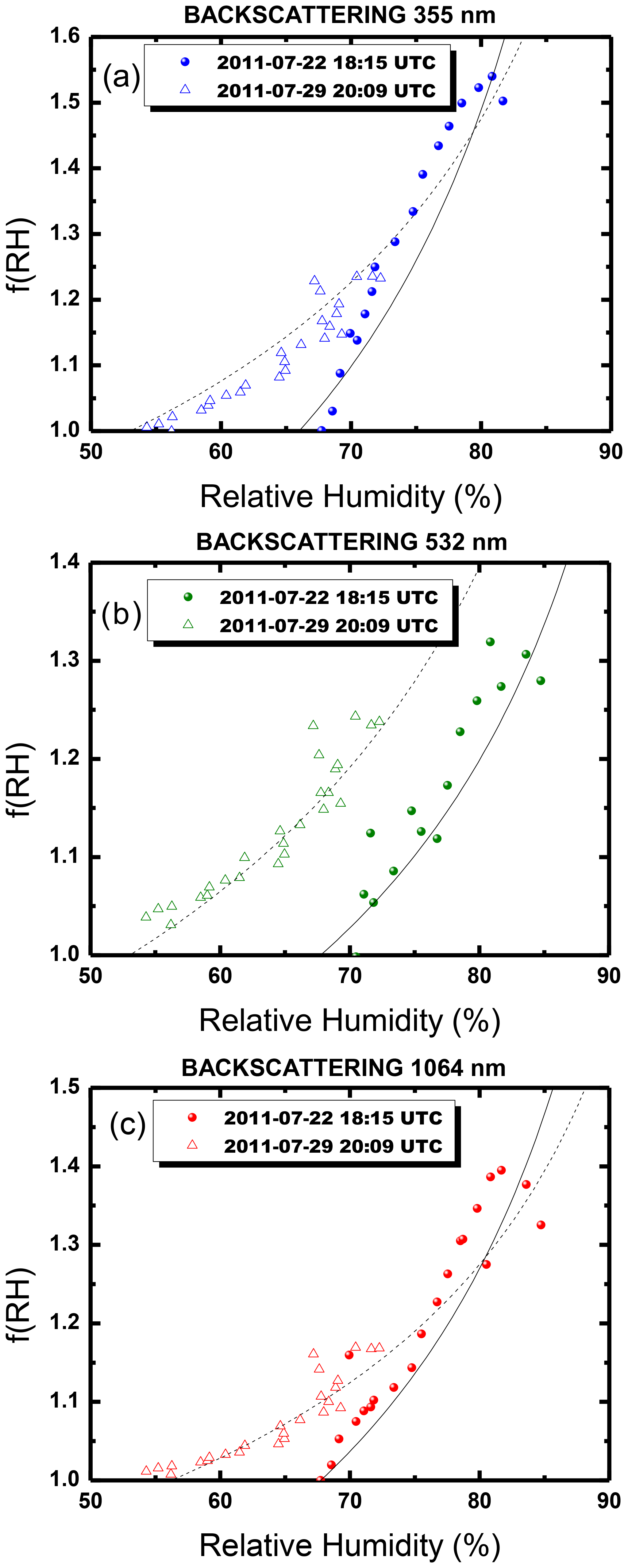
Figure 6Humidograms of f(RH) versus relative humidity for the aerosol backscattering data obtained on 29 and 22 July 2011. Data are presented at the wavelengths of (a) 355 nm, (b) 532 nm and (c) 1064 nm.
During the time that lidar data from Fig. 5 were acquired, the P-3B airplane performed spirals up and down over the GSFC/HUBC location. Figure 7 shows P-3B airborne measurements of hygroscopicity parameters γ and f(RH). The scattering coefficient at 532 nm (σdry – computed using Ångström law) and the number of particles obtained by the UHSAS (NUHSAS) instrument are also shown, both being computed at dry conditions. The most remarkable result from Fig. 7 is that for these four parameters there are no significant differences within the planetary boundary layer indicating well-mixed conditions required in our lidar analyses. Above these limits (∼ 2200 m on 29 July and ∼ 1800 m on 22 July), the hygroscopicity parameters are also stable although very noisy due to the considerably lower aerosol loads. Also, σdry and NUHSAS can be seen to decrease above the boundary layer from their approximately constant values below it. The only exception is on 22 July during the spiral up when a sharp increase in σdry and NUHSAS occurs near the top of the boundary layer, possibly due to accumulation of pollutants.

Figure 7Vertical profiles of hygroscopicity parameter γ and f(RH), scattering coefficient at dry conditions (σdry) and number of particles from UHSAS (NUHSAS) acquired from the P-3B airplane over the GSFC/HUBC region on the (a) 29 July spiral down, (b) 29 July spiral up, (c) 22 July spiral down and (d) 22 July spiral up.
We computed the mean aerosol parameters obtained by the P-3B in the planetary boundary layer, with the mean results being summarized in Table 2 (hygroscopicity parameters γ and f(RH), absorption (σabs,dry) and scattering (σscat,dry) coefficients and single scattering albedo (SSA) for dry conditions, and scattering coefficient for ambient conditions (σscat,amb)). All parameters are given at the reference wavelength of 532 nm. Similarly, results of microphysical parameters are summarized in Table 3 (number and volume of particles computed by SMPS, LAS, UHSAS and APS instruments). The very low standard deviations for all optical and microphysical parameters – except for (σscat,amb) – indicate well-mixed conditions in the planetary boundary layer required for lidar analyses.
Table 2Mean values in the planetary boundary layers of hygroscopicity parameters γ and f(RH), absorption (σabs,dry) and scattering (σscat,dry) coefficients and single scattering albedo (SSA) for dry conditions, and scattering coefficient for ambient conditions (σscat,amb). Reference wavelength for all aerosol optical parameters is 532 nm.
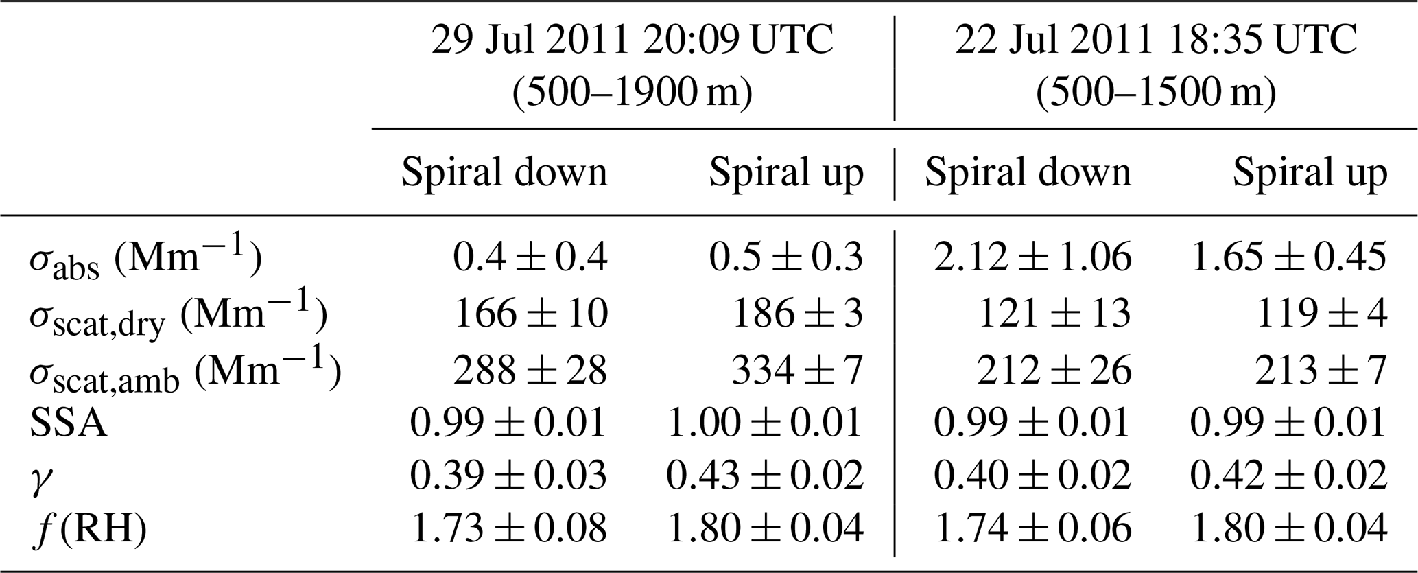
Table 3Mean values in the planetary boundary layers of total number of particles (N) and volume of particles (V) obtained by SMPS, UHSAS, LAS and APS instruments. Data are representative of dry conditions.
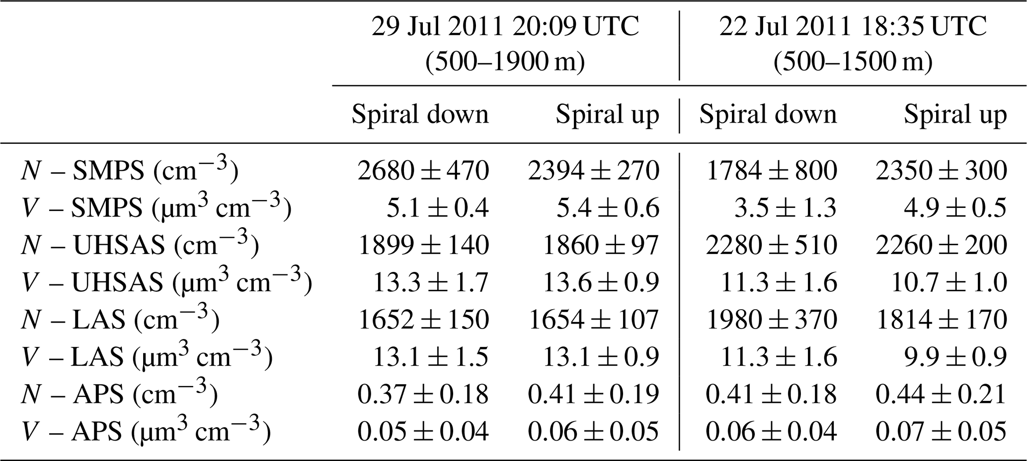
The most important finding is that when comparing γ parameters from the P-3B airplane in Table 2 with those obtained in Table 1 from lidar measurements (γ values of ∼ 0.39 at 532 nm derived from lidar parameters and of 0.39–0.43 from in situ airplane measurements), we observe very similar results with the differences below 5 %. The comparison for f(RH) between both methodologies also shows very good agreement. These results and the constant values of γ and f(RH) by the P-3B measurements serve as a validation of the methodology for characterizing aerosol hygroscopic effects on the aerosol vertical profiles using lidar measurements. The fact that the total number and volume of particles remains constant through the boundary layer supports the hypothesis of the same aerosol type in dry conditions with well-mixed atmospheric conditions. This last point agrees also with the constant σscat,dry, while the σscat,amb as computed with Eq. (1) yields profiles very similar to those of Fig. 5. Therefore, we conclude that aerosol hygroscopicity is the main cause of vertical changes in aerosol backscattering. The increase of extinction with height observed in Fig. 5 can be also associated with aerosol hygroscopic growth assuming the same Hänel parameters obtained.
Table 2 reveals that aerosol hygroscopicity is very similar between the two days studied with values of γ and f(RH) that agree to within 5 %. For both days, aerosol absorption was found to be negligible with SSA very close to 1. Also, essentially no variability was found in the absorption vertical profiles by the P-3B measurements (graphs not shown for brevity). Changes in scattering and extinction coefficients between both days can be explained by the different aerosol loads as indicated by the total number of particles shown. To investigate what aerosol types might have been present, Table 4 shows the mean mass of the different species measured by the PILS instrument. We note that for some species there are no measurements because their amount in the atmosphere was below the detection limit of the instrument and thus negligible. Also, the large integration time for obtaining the chemical composition did not allow the retrieval of vertical profiles at the resolution similar to that in Fig. 7. Indeed, the low standard deviations for each of the species again suggest a well-mixed layer below the top of the planetary boundary layer.
Table 4Mean values of total mass of the different species that form aerosol particles in the planetary boundary layers.
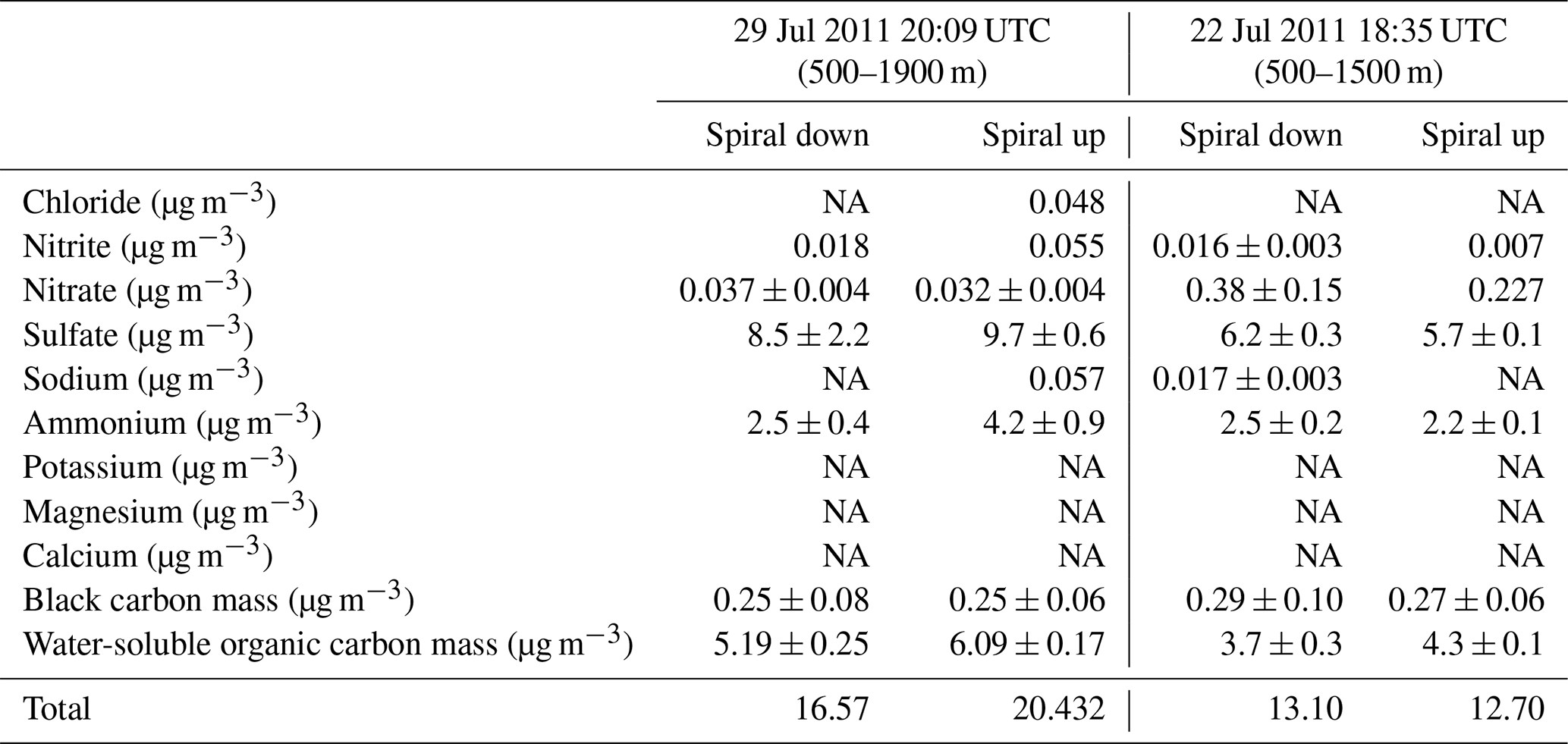
Table 4 reveals that sulfate is the predominant species for both days, with a percentage ranging between 45 %–52 % for the two days. Carbonaceous species (black carbon plus water-soluble organic carbon) are the second most prevalent, comprising 30 %–36 % of the total mass and particularly 93 % of that carbonaceous species are water-soluble organic carbon. Sulfate and water-soluble organic carbon are hydrophilic and explain the large effect of aerosol hygroscopicity on aerosol properties over the study region. Other important species that were present are ammonium with a percentage of 15 %–20 %. The rest of the species are generally negligible, with nitrates being only of interest at 3 % of total mass on 22 July.
To further study the present cases, retrievals of aerosol microphysical properties from 3β+2α lidar measurements were made using case-dependent optimized constraints (Pérez-Ramírez et al., 2019), which for the data of Fig. 5 were of low absorption (mi,max=0.01, mr,max=1.45) and fine-mode predominance (rmax=2 µm). Figure 8 shows the main results of bulk parameters (effective radius (reff), aerosol volume (V) and number concentrations (N)) and real refractive index, both for 29 July (Fig. 8a–d) and 22 July (Fig. 8e–f). Because of the use of case-dependent optimized constraints, results are representative of fine-mode aerosols and uncertainties are of ∼ 25 % for reff and V and of ∼ 100 % for N (Pérez-Ramírez et al., 2013), while for mr they are ±0.05 (Pérez-Ramírez et al., 2020). Figure 9 shows particle volume size distributions for different representative altitudes both below and above the planetary boundary layer, but we note that particle size distributions obtained by the stand-alone 3β+2α lidar inversion can possess significant errors of up to 100 % (e.g., Veselovskii et al., 2004).
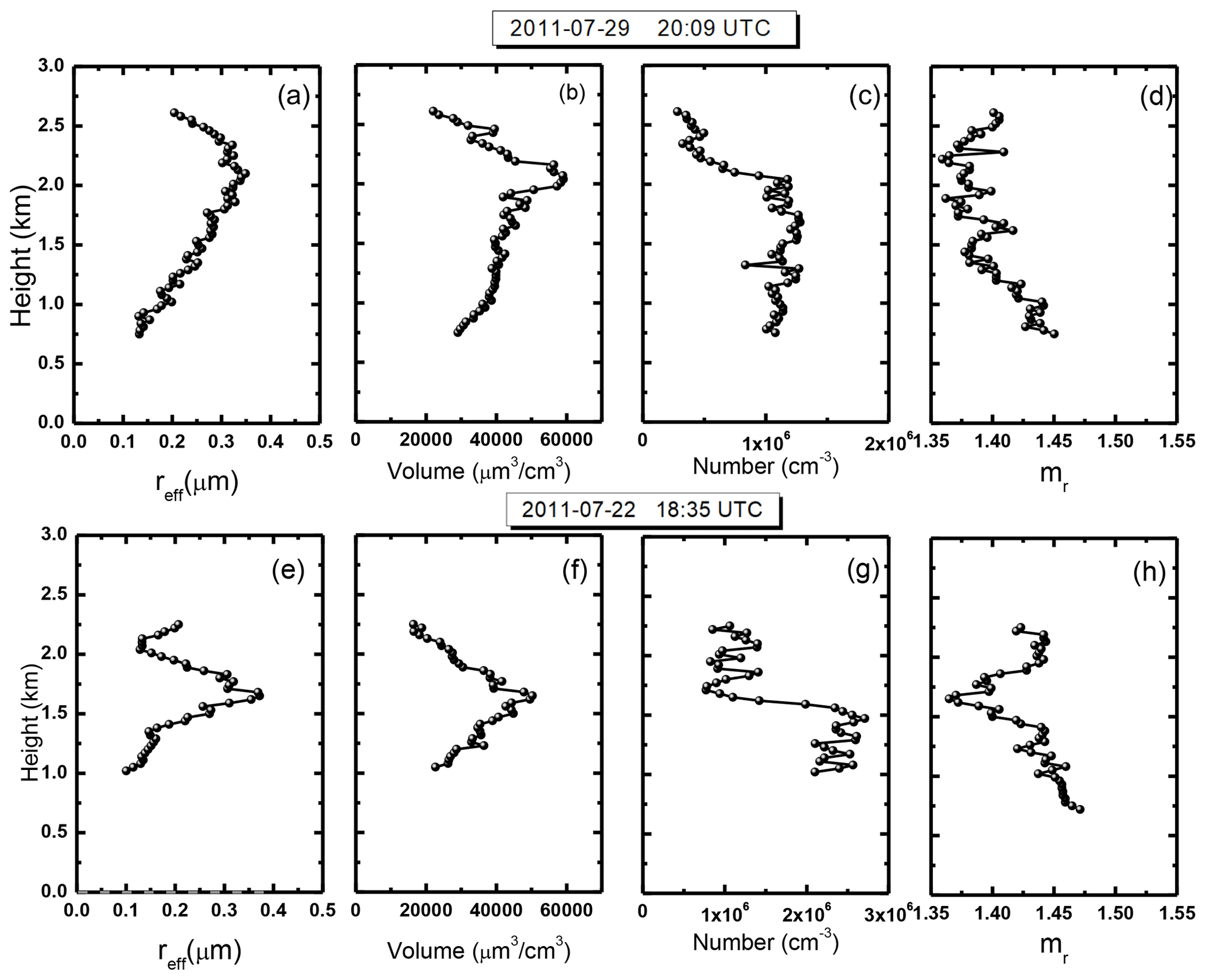
Figure 8Retrieved effective radius (reff), volume and number concentrations and real part of refractive index (mr) from the stand-alone 3β+2α lidar inversion for (a–d) 29 July 2011 and (e–f) 22 July 2001.
Referring to Fig. 8, on both days, reff shows an increase with altitude from values of ∼ 0.12 µm at 1 km altitude to values around 0.3–0.35 µm at the top of the boundary layer when maximum hygroscopic growth was achieved. Above the planetary boundary layer, the decrease of reff with altitude is clear because above this level relative humidity drops drastically, thus eliminating hygroscopic growth. For volume concentration, Fig. 8 reveals an increase with altitude that is consistent with the increase of extinction with altitude and with the changes in particle volume size distributions. We note that now volume concentration is for ambient conditions, while the results obtained from P-3B measurements were for dry conditions, which explains the differences with altitude. For number concentrations, which is the parameter with the largest error of ∼ 100 % (Whiteman et al., 2018), a pattern with approximately constant values is observed in the planetary boundary layer in agreement with the expectation of approximately the same number of particles for well-mixed conditions. Finally, for mr, we observe a decrease with altitude from values ∼ 1.45 to values close to ∼ 1.35, which is typical for hydrated particles. We note that retrieved mi was below 0.005 for all cases which produced high SSA (>0.98). The range of retrieved reff, refractive indices and SSA are typical of a mixture of sulfate and water-soluble organic carbon (e.g., Chin et al., 2002), which is the predominant chemical composition from Table 4.
Figure 9 illustrates the displacement of size distribution to a large radius with altitudes within the boundary layer, which is the typical pattern expected (e.g., Schafer et al., 2008) and agrees with the increase in radius with altitude observed in Fig. 8 and associated with hygroscopic growth. The size distributions in Fig. 9 suggest a second fine mode (particles with radius below 0.5 µm) which could be an indication of aerosol–fog modification (e.g., Eck et al., 2012) although such a conclusion must be considered tentative due to uncertainties (∼ 100 %) in the retrieved size distribution. Above the planetary boundary layer, the size distributions are clearly displaced toward smaller radii.
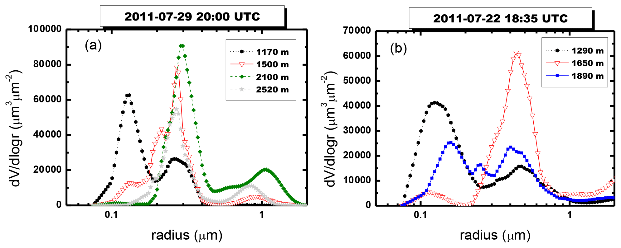
Figure 9Particle volume size distributions at different levels obtained from the stand-alone 3β+2α lidar inversion for (a) 29 July 2011 and (b) 22 July 2001.

Figure 10Temporal evolution of aerosol extinction coefficient (α) at 532 nm obtained by the HSRL-1 system over the Baltimore–Washington DC area on (a) 29 July 2011 and (b) 22 July 2011. Vertical white lines represents times when the system flew over NASA Goddard Space Flight Center.
3.3 Aerosol spatial distribution through the day
Airborne measurements acquired by the HSRL-1 system provided extended records of the evolution of aerosol vertical distribution during the field campaign. For example, Fig. 10 shows more than 8 continuous hours of α(532 nm) from HSRL-1 measurements on 29 and 22 July. Data shown in Fig. 10 are only cloud-free data with vertical white lines illustrating the times when the aircraft flew over NASA GSFC. The large gaps around 19:00 UTC on 29 July and 17:00 UTC on 22 July are when the UC-12 airplane landed and refueled between the morning and afternoon flights, while the small gaps correspond to cloud-filtered data.
For 29 July at 18:00 UTC, Fig. 10a reveals some decoupled aerosol layers within the planetary boundary layer that agrees with the patterns observed in Fig. 4. After that time, there are many cloud-filtered data that agree with the convective clouds observed in Fig. 4 as well. In particular, it should be noted that the aircraft measurements reveal that after approximately 19:00 UTC on both days, there were increases of aerosol extinction with height within the planetary boundary layer. These increases agree again with those observed in Fig. 4 and can be associated with aerosol hygroscopic growth. On the other hand, data from Fig. 10b complement the sparse data obtained from ground-based lidar measurements on 22 July. Again, some decoupled aerosol layers are observed early in the morning. But on that day, there were more cloud-affected data. Nevertheless, after 18:00 UTC, an increase in α with height is again observed within the planetary boundary layer consistent with the aerosol hygroscopicity previously studied. For much of the HSRL-1 datasets on 29 and 22 July, daytime well-mixed conditions associated with convective processes were present with relative humidity increasing with altitude (Fig. 3). Also, chemical composition measurements revealed the presence of hygroscopic aerosols (Table 4). Therefore, the similarity in aerosol vertical distribution patterns between both days can be interpreted as indicating the presence of swelling aerosols resulting in an aerosol profile characterized by an increase in backscattering and extinction with height. Based on the aircraft measurements, we take that pattern to be representative of the extended area and not just over the specific ground-based lidar site.
The analyses of the in situ measurements taken from the P-3B aid the understanding of aerosol hygroscopic effects. Figure 11 shows mean hourly values of αamb(532 nm), γ and f(RH) for both 29 and 22 July. We note that the values of αamb(532 nm) are computed by adding the absorption coefficient to σamb(532 nm) which is obtained using Eq. (1) from the measured σdry(532 nm), γ and relative humidity. Data are presented for three different altitudes: near the surface (altitude below 1 km), in the planetary boundary layer (1–2 km for 29 July and 1–1.8 km for 22 July) and above the planetary boundary layer (>2.0 km for 29 July and >1.8 km for 22 July). Single scattering albedo was also measured by P-3B in situ instrumentation, but for all cases values obtained were above 0.98, making absorption negligible. The P3-B also incorporates measurements of relative humidity, but these measured values are basically the same than those obtained by radiosondes in Fig. 3 (differences are within the uncertainties of the methods). The analyses of αamb(532 nm) clearly reveals the importance of hygroscopic growth as ambient values are generally 1.8 times the dry values, which is consistent with the measured f(RH). Generally, the larger values of αamb(532 nm) are obtained in the altitude range considered to be in the planetary boundary layer, which is consistent with the previous finding of larger extinction in that region due to hygroscopic growth for the atmospheric conditions present on both days (Fig. 3). Also, both days show that below the top of the boundary layer, αamb(532 nm) is approximately constant for both dry and humid conditions, but above the boundary layer there is an increase with time after 20:00 UTC for 29 July – the lack of data for these times on 22 July may suppress that pattern. Actually, the fact that the last measurement at 22:00 UTC above the boundary layer has larger extinction values than the rest can be explained by the increase of PBL height (see Fig. 10a), and thus the P3B airplane is sampling the swollen aerosols that earlier in the day were not sampled.
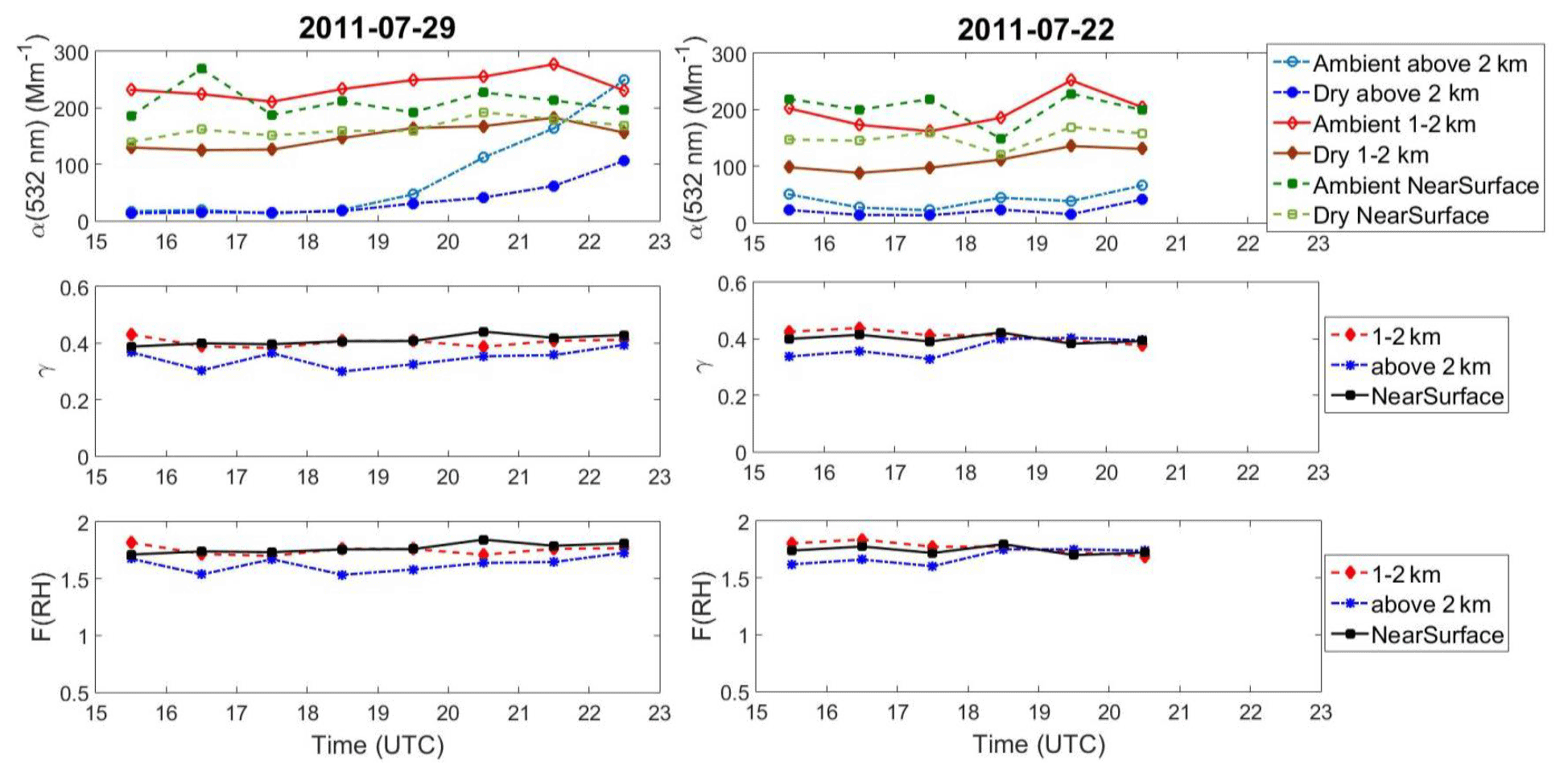
Figure 11Hourly mean values of aerosol extinction at 532 nm (α(532 nm)) and hygroscopicity parameters γ and f(RH) for both 29 and 22 July. Data are presented for three different altitudes: near the surface (altitude below 1 km), in the planetary boundary layer (1–2 km for 29 July and 1–1.8 km for 22 July) and above the planetary boundary layer (>2.0 km for 29 July and >1.8 km for 22 July).
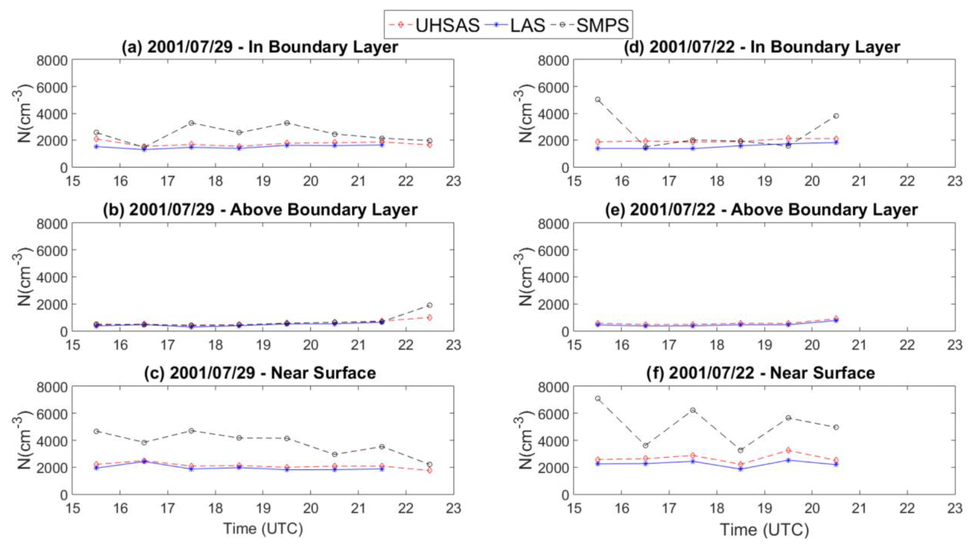
Figure 12Hourly mean values of mass of the different species that form aerosol particles measured by the P-3B airplane on 29 and 22 July 2011. Data are presented for three different altitudes: near the surface (altitude below 1 km), in the planetary boundary layer (1–2 km for 29 July and 1–1.8 km for 22 July) and above the planetary boundary layer (>2.0 km for 29 July and >1.8 km for 22 July).
Another important result from Fig. 11 is that during the entire day there are relatively constant values of γ (∼ 0.35–0.41) and f(RH) (∼ 1.6–1.8) for both days. This implies that hygroscopic aerosols were present during the entire measurement periods and over the broad study region, and the combination of the well-mixed atmospheric conditions layers and increasing relative humidity with height created the conditions for aerosol swelling and the increase in aerosol backscattering and extinction with height. These conditions are found typically in the afternoon/evening and are associated with convective conditions. Early in the morning, the hygroscopic growth can also be present but because of the lack of well-mixed conditions the effect on atmospheric extinction and backscattering cannot be predicted using the procedure here and depends on the characteristics of each day.
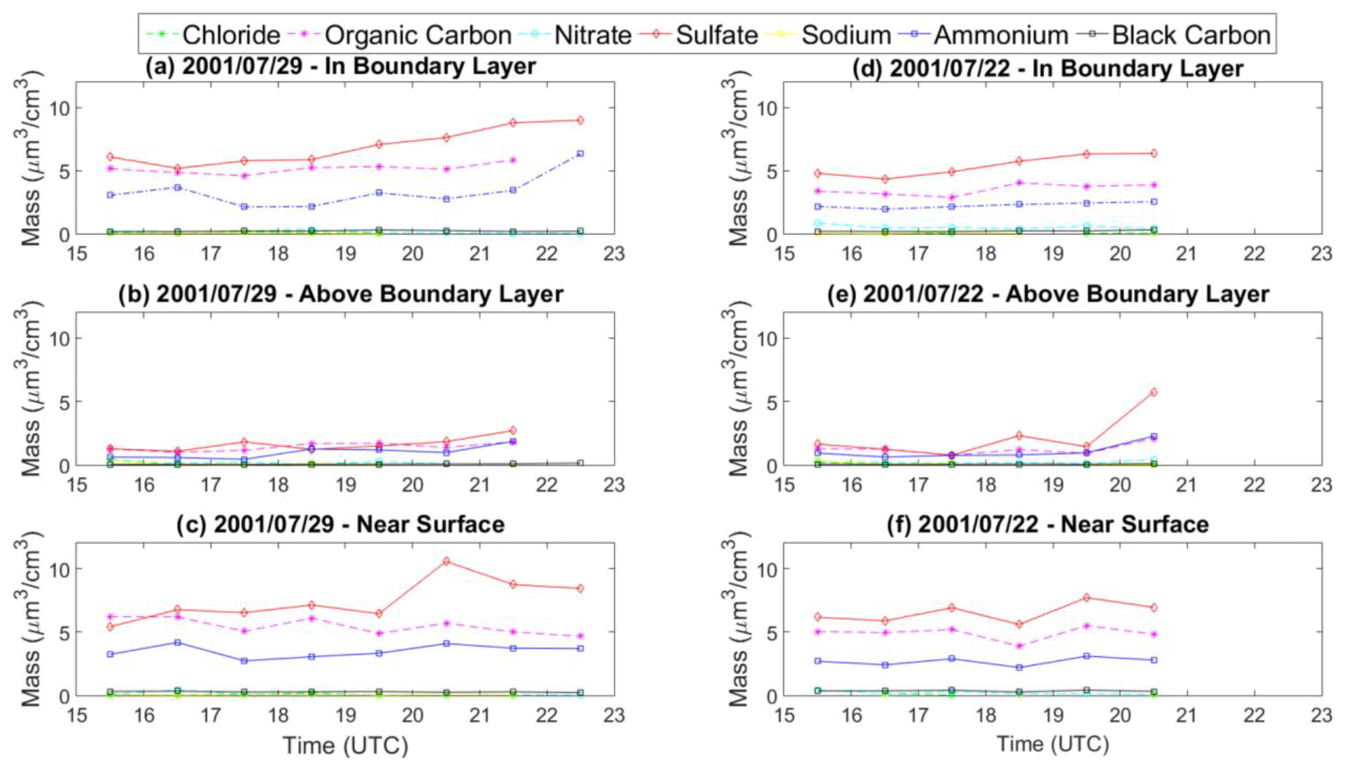
Figure 13Hourly mean values total number of particles obtained by the SMPS, UHSAS and LAS instruments aboard the P-3B airplane and acquired on 29 and 22 July 2011. Data are presented for three different altitudes: near the surface (altitude below 1 km), in the planetary boundary layer (1–2 km for 29 July and 1–1.8 km for 22 July) and above the planetary boundary layer (>2.0 km for 29 July and >1.8 km for 22 July).
Figure 12 shows the hourly mean number of particles obtained from the P-3B for the same vertical intervals as in Fig. 11. Both UHSAS (radius between 0.06–1 µm) and LAS (radius between 0.9–7.7 µm) measure about the same number of particles and the patterns of the values from both instruments are very similar near the surface and in the planetary boundary layer with stable values through the entire measurement period. These results are consistent with those from Fig. 8 and imply that a similar concentration of particles was present in the atmosphere during the day and that changes in aerosol extinction, backscattering and AOD are explained by aerosol hygroscopicity. Above the planetary boundary layer, the number of particles drops drastically and, as seen in Fig. 3, the relative humidity drops significantly. Finally, it is important to note that the SMPS always indicates a larger number of particles than for UHSAS and LAS which shows significant variability during the day, particularly for 29 July. But the SMPS is representative of ultrafine particles (radius between 10–300 nm) that are not detected by lidar measurements because of the lack of counting efficiency at the emission lidar wavelengths and comparisons are not straightforward.
The evolution of chemical composition of aerosol particles serves to better understand aerosol hygroscopicity for the two study days. Figure 13 shows hourly means of the main species (mass above 0.03 µg m−3). As in the previous figures, data are shown for near the surface, in the planetary boundary layer and above the planetary boundary layer. For any day and layer, sulfate is by far the predominant species followed by water-soluble organic carbon and ammonium. As we saw in Table 4, these species are highly hygroscopic and explain the aerosol hygroscopicity previously observed. The total mass is stable throughout the day except for a slight increase in sulfate total mass after 18:00 UTC which can be explained as an accumulation of sulfate particulate due anthropogenic emissions during the day (e.g., Fitzgerald et al., 1982). Ammonium also shows a very slight increase late in the evening for 29 July. We note that standard deviations of mean values were below 10 %, confirming the stability in mass amount and percentage and implying that the results are representative of the entire study region. Therefore, assuming that sulfate, ammonium and water vapor organic carbon emissions are of anthropogenic origin, we can conclude that the impact of these emissions on aerosol backscattering and extinction profiles and eventually on AOD is enhanced by aerosol hygroscopicity.
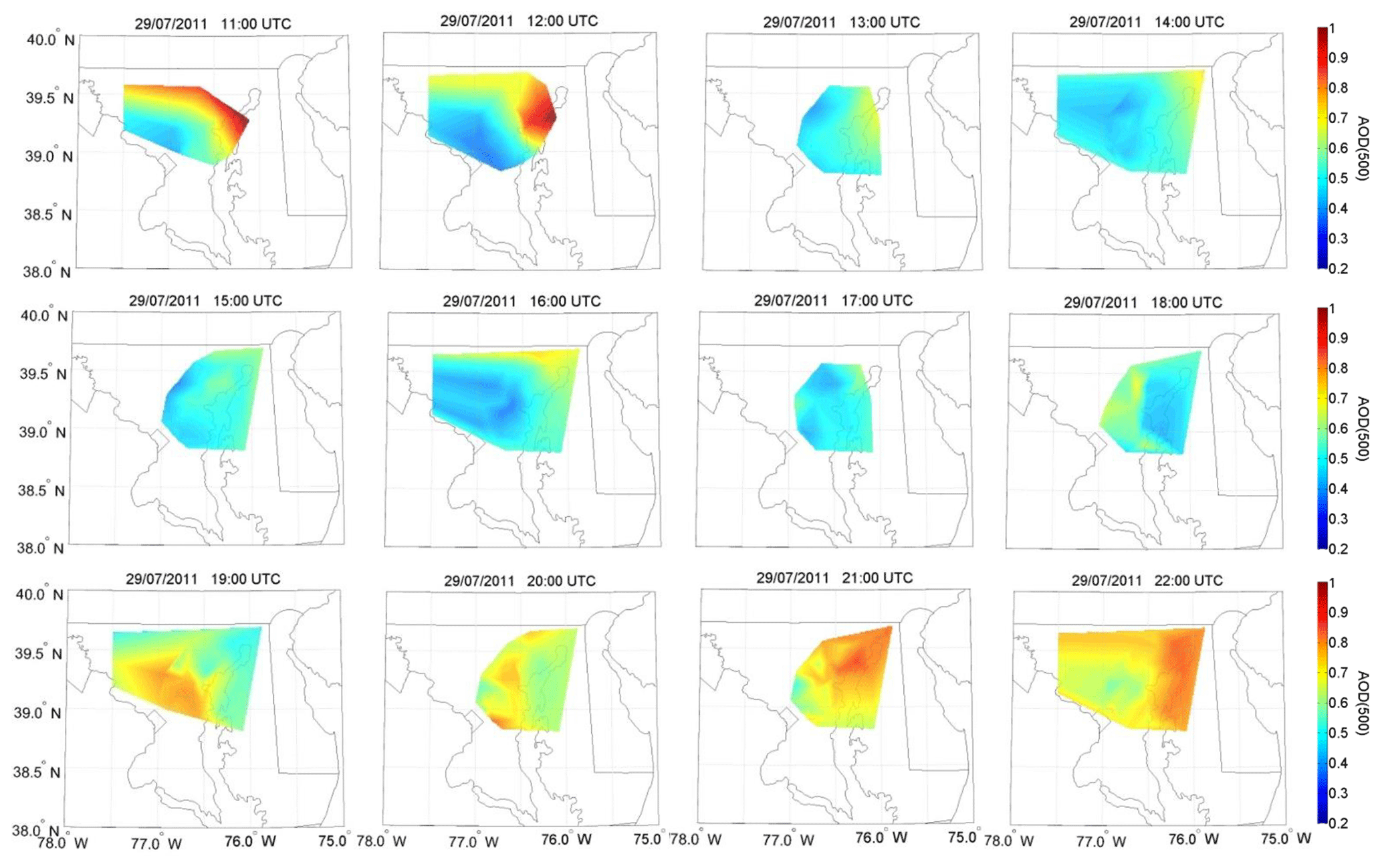
Figure 14Temporal evolution of AOD at 500 nm from AERONET-DRAGON over the Baltimore–Washington DC area on 29 July 2011.
The large number of stations deployed by AERONET-DRAGON permits us to study how aerosol hygroscopicity affected AOD, representative of the entire column, over the study region. Figure 14 shows the color map of hourly mean AODs for the Baltimore–Washington DC region on 29 July 2011. We performed gridded linear interpolations between the stations to obtain the color maps shown (see Fig. 1c for an illustration of the AERONET-DRAGON stations). We note that the number of stations for the interpolations differed among different hours because of the presence of partly cloudy skies that obscured the Sun and thus prevented AERONET-DRAGON measurements from being performed. What Fig. 14 clearly reveals is an increase in AOD throughout the day, reaching the maximum values in the evening (AOD ∼ 0.7–0.8) in spite of some spikes in the northern locations that could be associated with automobile traffic or other local anthropogenic emissions in the region. The evening values of AOD can be as much as twice those in the early morning. If we assume that atmospheric conditions from Fig. 3 can be extrapolated to the entire region, then the well-mixed conditions during the evening can better explain the more regionally uniform AOD values than those obtained during the morning.
The spectral deconvolution algorithm (O'Neill et al., 2003) was used to separate AOD into fine- (AODfine) and coarse-mode (AODcoarse) contributions. Figure 15 displays AODfine temporal evolution for 29 July 2011 (AODcoarse graphs not shown for brevity). Again, the figures show the values for the entire Baltimore–Washington DC region, and data were gridded using linear interpolations. The similarity of Figs. 14 and 15 indicates a predominance of AODfine over AODcoarse during the entire day. Actually, AODcoarse was mostly below 0.06 – with some exceptions in the northern locations in the morning perhaps due to local sources (e.g., road traffic) but not representative of the entire region. The values of AODfine are comparable to those of total AOD and were seen to increase during the day, with larger values during the evening (∼ 0.7–0.8) than during the morning (∼ 0.4–0.6). These patterns reveal that the increase in the AOD during the day can be associated mainly with changes in the fine mode. But now, combining the information of aerosol hygroscopicity previously obtained from lidar measurements and from the analyses of aerosol hygroscopicity in Sect. 3.2, we can conclude that changes in the AOD during the day can be mainly associated with changes induced by aerosol hygroscopicity that occurred when well-mixed conditions were achieved. We conclude that these changes in the AOD occurred over an extended region. Similar patterns in AOD were obtained for 22 July but the graphs are not shown for brevity. However these results are just an illustration of the predominant mechanism in AOD increase during the day because of some relative increase of pollutants such as sulfate particles (Fig. 13).
Figure 16 shows hourly mean volume aerosol size distributions from AERONET-DRAGON Level 2.0 data, both for 29 and 22 July. Unfortunately, due to partly cloudy skies, there were some times during the day when there were no retrievals, particularly on 22 July. Nevertheless, the volume size distributions clearly illustrate an increase in the fine mode for both days that is responsible for majority of the total increase in aerosol AOD during the day.
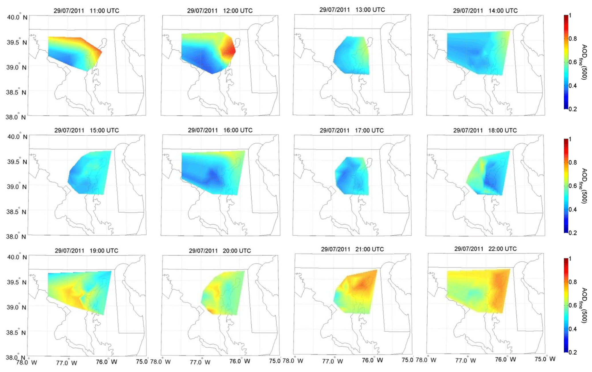
Figure 15Temporal evolution of fine-mode aerosol optical depth (AODfine) at 500 nm from AERONET-DRAGON over the Baltimore–Washington DC area on 29 July 2011.
Mean optical and microphysical results obtained from AERONET Level 2.0 inversions are summarized in Table 5 differentiating between morning (before 13:00 UTC) and evening (after 19:00 UTC) values. Also, results in Table 5 are shown for 532 nm using linear interpolations between retrieved values at 440 and 670 nm, since no significant wavelength dependence was found. For mr, the retrieved values are between 1.36 and 1.39 and are typical of highly hydrated particles. The very low values of mi (≤0.003) and high values of SSA (≥0.98) indicate that absorption is negligible as well. All of these values of refractive index and SSA are typical for highly hydrated particles (e.g., Chin et al., 2002). For the microphysical properties, the effective radius is also relatively high, although it is within the fine mode (reff ∼ 0.23–0.25 µm). Values of rfine are similarly high (∼ 0.17 µm). But these ranges of reff and rfine are typical of a size distribution of highly hydrated particles (e.g., Dubovik et al., 2002; Pérez-Ramírez et al., 2017). The predominance of Vfine over Vcoarse is clear, implying a negligible coarse mode. But AERONET retrievals do not show significant differences between morning and evening values and do not refer significant differences associated with the presence or lack of hygroscopic growth, as revealed by Figs. 14 and 15. The large number of stations together with the errors associated with AERONET inversions can mask temporal changes with relative humidity. Another point is that AERONET retrievals are effective values representative of the entire atmospheric column, which can mask specific variations in aerosol microphysical properties with altitude. Nevertheless, it should be noted that AERONET-retrieved parameters and those from stand-alone 3β+2α lidar inversion shown in Fig. 8 are consistent with each other and representative of aerosol hygroscopic growth. Therefore, the combined lidar and AERONET retrievals presented serve to further understand changes in aerosol microphysical properties with relative humidity.

Figure 16Mean hourly values of aerosol size distributions from AERONET-DRAGON stations over the Baltimore–Washington DC region on (a) 29 July 2011 and (b) 22 July 2011.
Table 5Mean real refractive index (mr), imaginary refractive index (mi), single scattering albedo (SSA), asymmetry factor (g), effective radius (reff), particle volume (V), fine-mode radius (rfine) and volume (Vfine) and coarse-mode radius (rcoarse) and volume (Vcoarse) obtained from AERONET Level 2.0 inversions on 29 and 22 July 2011.

3.4 Aerosol radiative impact
Figure 17 shows ARE profiles, while Fig. 18 shows the HR profiles, for both 22 and 29 July 2011. In the figures, AREs are represented both differentiating among the wavelengths of lidar measurements (355, 532 and 1064 nm) and the integrated values for the shortwave region (280–3000 nm). The computations were done using libRadtran following the configuration described in Sect. 2.4 and using the 3β+2α vertical profiles for the hygroscopic growth cases illustrated in Fig. 5. Inputs of temperature and humidity profiles were those obtained from radiosonde measurements launched very close in time with lidar measurements (Fig. 3). Extinction and backscattering measurements at ambient conditions were used in the computations. But the equivalent backscattering profiles for “dry” conditions were computed using the Hänel equations (Eq. 5) and the corresponding “γ(λ)” obtained in Fig. 6 and RH measurements, where the reference values βref and RHref were those obtained at the lowest altitude. For the extinction profiles at dry conditions, we used again the Hänel equation but replaced backscattering by extinction and assumed the same hygroscopic growth factor “γ(λ)”. For the incomplete overlap region (approximately the first kilometer), α and β were computed using the Hänel equation with the hygroscopicity parameters “γ(λ)” and the measured RH in this first kilometer. Below 3 km where most of the aerosol was found, for 22 July, the obtained aerosol optical depths at 355 and 532 nm were approximately 0.50 and 0.36 for ambient conditions and of 0.33 and 0.27 for dry conditions, while for 29 July the AODs were approximately 0.95 and 0.57 for ambient conditions and 0.76 and 0.4 for dry conditions. Solar zenith angles were 23.24∘ for 22 July and 42.69∘ for 29 July. Because we are using the same methodology for ARE computations, possible differences in ARE computations between ambient and dry conditions for the same profile should be independent of the errors associated with the methodology for ARE computations (e.g., Sicard et al., 2014; Granados-Muñoz et al., 2019).
Figure 17 clearly demonstrates a wavelength dependence of ARE for both days, with the largest cooling effect obtained at 532 nm on both days followed by 355 nm. Actually, systematic lower values of ARE are observed at ambient conditions below the top of the PBL. At the surface, the differences of ambient minus dry AREs are the largest and take values of −17.4 and −13.2 mW m2 nm−1 at 532 and 355 nm for 22 July and of −30.85 and −11.2 mW m2 nm−1 at 532 and 355 nm for 29 July. The systematic lower values of ARE (in absolute value) for 29 July are explained by the larger aerosol load and solar zenith angle for that day. Above the PBL, there are no important differences between ambient and dry profiles for any wavelength (values of ∼ 2.5 mW m2 nm−1 at 532 nm and ∼ 3.5 mW m2 nm−1 at 355 nm), with differences between both days negligible. Values at 1064 nm are basically zero for both days both for ambient and dry conditions independently of altitude, and therefore we can conclude that ARE for these types of particles (mixture of sulfates and water-soluble organic carbon) is only sensitive in the visible and UV region. This has to be taken into account when analyzing the SW profiles that reported an important difference between ambient and dry profiles where the maximum difference is at the surface (approximately of −10 and −7 mW m2 on 29 and 22 July, respectively) and minimum close to zero near the top of the PBL. Actually, above these altitudes, small constant values are observed with height with no differences between dry and ambient conditions. Therefore, we conclude that aerosol hygroscopic growth is the cause of the larger cooling effect for the types of particles analyzed here. Comparisons of ARE with other aerosol types are not straightforward because of the dependences with AOD, aerosol single scattering albedo and asymmetry parameter and solar zenith angle, although the reported cooling effects agree with other studies (e.g., Di Biagio et al., 2009; Huang et al., 2009; Bhawar et al., 2016; Mallet et al., 2016; Wang et al., 2020)
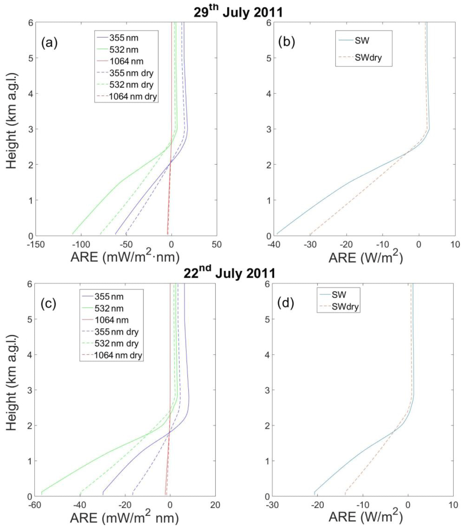
Figure 17Vertical profiles of aerosol ARE from the lidar measurements affected by aerosol hygroscopic growth. Data are presented (a, c) for the measured lidar measurements (355, 532 and 1064 nm) and (b, d) integrated for the shortwave range (280–3000 nm).
Figure 18 also shows a wavelength dependence in HRs below the PBL with positive values above K d−1 for 355 and 532 nm, with HRs very close to zero at 1064 nm. For the aerosol-free region above the PBL, the computed HRs are basically zero for all wavelengths. The maximum differences between ambient and dry conditions are found for 355 and 532 nm in the region close to the top of the PBL where there was more hygroscopic growth. These differences between ambient and dry conditions are approximately and K d−1 at 532 and 355 nm for 22 July and of and K d−1 at 532 and 355 nm for 29 July. The integrated SW values show similar patterns on both days with an increase from minimum values at the surface (∼ 0.05 K d−1) to maximum values near the top of the PBL where the differences between ambient and dry conditions are maximized (∼ 0.12 K d−1) and associated again with aerosol hygroscopic growth. These positive HRs for the SW region agree with other studies (Mallet et al., 2008; Lemaitre et al., 2010; Perrone et al., 2012; Meloni et al., 2015; Granados-Muñoz et al., 2019), although the aerosol types in this study are different.
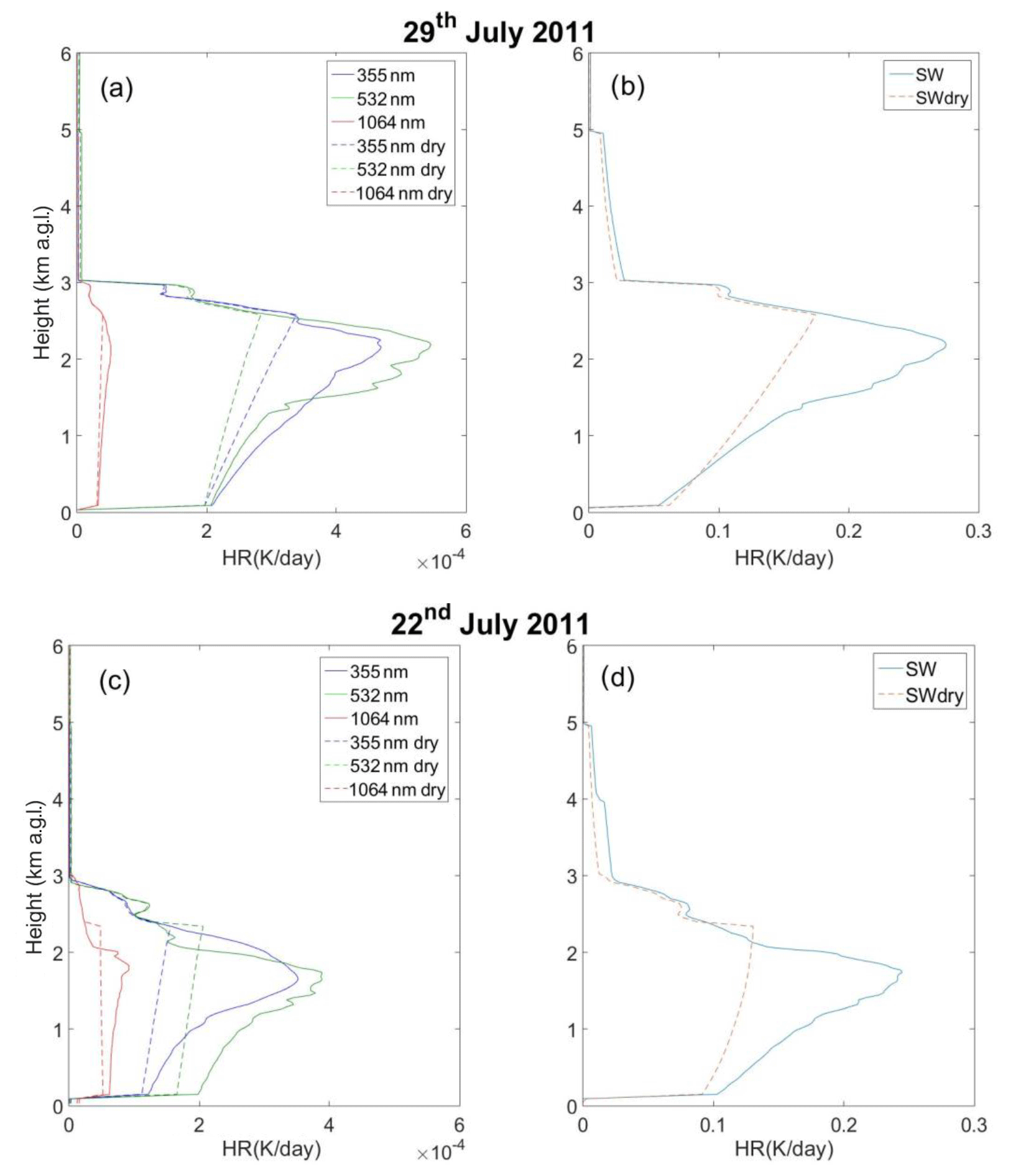
Figure 18Vertical profiles of aerosol heating rates from the lidar measurements affected by aerosol hygroscopic growth. Data are presented for the measured lidar measurements (355, 532 and 1054 nm) and integrated for the shortwave range (280–3000 nm).
This work has focused on the study of aerosol hygroscopic properties during the DISCOVER-AQ 2011 field campaign in the Baltimore–Washington DC metropolitan area. During the campaign, a unique dataset was available: the NASA P-3B airplane deployed in situ instrumentation that permitted the characterization of aerosol hygroscopic growth and other aerosol optical, microphysical and chemical properties, while the HSRL-1 lidar system was deployed on the NASA UC-12 airplane for continuous characterization of backscattering (β) and extinction (α) profiles at 532 nm. Ground-based measurements included the multiwavelength Raman lidar at NASA GSFC that acquired independent profiles of aerosol extinction and backscattering at 355 nm. Both the Raman and HSRL-1 systems obtained aerosol backscattering at 1064 nm. Combined Raman and HSRL-1 measurements made during UC-12 overpasses at GSFC provided the 3β+2α configuration used for the retrieval of vertically resolved aerosol microphysical properties, and the study presented here serves to complement the hybrid configuration of lidars presented by Sawamura et al. (2014) over the same region. The deployment of AERONET-DRAGON with more than 40 instruments in the region permitted a continuous characterization of columnar aerosol properties and the study of their spatial representativeness and variability.
For the study of aerosol hygroscopic growth with lidar measurements, stable and well-mixed conditions were needed. Radiosondes launched from HUBC permitted the characterization of the state of temperature and humidity in the atmosphere every four hours, and cases that fulfill the previous conditions and with available lidar measurements were identified for 22 and 29 July 2011. The focus of the study was on 29 July because multiwavelength Raman lidar measurements were available for approximately 10 daytime hours. On 22 July, only 1.5 h of Raman measurements were available and thus only serve to complement the results of the other day. On both days, air masses had their origin close to the Ohio River Valley and there was no significant transport of aerosol at altitudes above the planetary boundary layer (PBL). Mean daily AODs at 500 nm were approximately 0.52 for 29 July and 0.42 for 22 July, with both days having an Ångström exponent of ∼ 1.8. The thermodynamic state of the atmosphere was characterized by well-mixed conditions in the afternoon below the top of the planetary boundary layer, with stable water vapor mixing ratio and relative humidity increasing from the surface (30 %–40 %) up to the top of the planetary boundary layer (values between 80 %–90 %).
For the study of aerosol hygroscopicity the Hänel equation, f(RH) = ((1-RH) (1-RHref))−γ, was used, with f(RH) being the ratio between humid (βamb) and the reference dry (βref) backscattering coefficients, RH and RHref the relative humidity both at ambient and reference conditions, and γ the hygroscopicity factor that depends on the type of particles. From lidar measurements, linear fits were performed by taking logarithms of both sides of the Hänel equation to obtain γ where the lowest height with measured backscattering was taken as the reference to compute βref and RHref. Computations of γ revealed a wavelength dependence for 355, 532 and 1064 nm of 0.46, 0.39 and 0.31 on 29 July and of 0.65, 0.38 and 0.37 on 22 July, although close to the uncertainty of the method that was demonstrated to be approximately 15 % through different simulations. These values of γ were confirmed by correlative spirals at GSFC by the P-3B using a pair of nephelometers that provided mean values of ∼ 0.41 at 532 nm, with the lidar retrieved values of γ agreeing within the estimated uncertainties of 15 %. Measurements performed by the P-3B airplane revealed that during the lidar measurements predominant aerosol chemical composition was sulfate and water-soluble organic carbon. Chemical composition was stable with altitude even though the large temporal resolution (∼ 15 min) compared to lidar measurements. Therefore, these results serve as validation of measurements of aerosol hygroscopicity from lidar measurements and confirm that the increase of aerosol backscattering with height measured by lidar measurements was due to aerosol hygroscopic growth effects associated with sulfates and water-soluble organic carbon. The extinction coefficients were observed to increase with altitude, which can be also explained by the effects of aerosol hygroscopicity.
The 3β+2α lidar measurements obtained by the combination of ground-based Mie–Raman and airborne HSRL-1 lidar systems during periods of aerosol hygroscopic growth were used as inputs to the regularization technique to retrieve aerosol microphysical properties. Effective radius (reff) showed an increase with altitude from dry values around 0.10–0.15 µm to humidified values of 0.30–0.4 µm. Volume concentration showed an increase with height similar to that of the extinction coefficients. Number concentration remained constant, which agreed with the hypothesis of the same number of particles under well-mixed conditions, and the same was found by P-3B measurements. The real refractive index (mr) showed a decrease with height from dry values of 1.45–1.50 to humidified values near to 1.35, which are the typical for highly hydrated particles. SSA both for dry and humidified conditions was above 0.99, which indicates essentially no absorption. The complementary chemical analyses by P-3B indicated that the predominant species were sulfate and water-vapor-soluble organic carbon, which are known to be highly hygroscopic and non-absorbing. Therefore, the combination of 3β+2α lidar retrievals with airborne measurements provided a unique closure study for aerosol hygroscopic growth characterization.
The analyses of AERONET-DRAGON data reported an increase of AOD throughout the day particularly for the fine mode. This was observed for the entire Baltimore–Washington DC metropolitan area. In spite of partly cloudy skies, the large number of instruments deployed provided sufficient AERONET inversions to obtain mean mr∼1.38, reff ∼ 0.24 µm and SSA ∼ 0.98 that are consistent with these obtained by lidar retrievals and confirmed aerosol hygroscopic growth over the region. On the other hand, P-3B measurements during the entire day reveal the same Hänel hygroscopicity parameters with time and altitude, which confirms that aerosol hygroscopicity was present during the entire day. The P-3B measurements also indicated an approximately constant number of particles and concentration of main species (sulfate and water-soluble organic carbon) during the day. Thus, combining all of AERONET-DRAGON, P-3B and lidar suggests that the increase of AOD during the day and the increase of aerosol backscattering and extinction with height can be directly associated with aerosol hygroscopic growth.
Through the use of the Hänel equations, assuming the same hygroscopic growth parameters γ(λ) for extinction and backscattering and with the relative humidity profiles, it was possible to compute extinction and backscattering coefficients for both ambient and dry conditions. This permitted the isolation of the effect of aerosol hygroscopicity and the study of their impacts on AREs and HRs, which were computed using the libRadtran radiative transfer code. Computations revealed a cooler surface for the shortwave range (differences between 7–10 W m−2 depending on aerosol load) and a larger heating near the top of the PBL (differences of approximately 0.12 K d−1) directly associated with aerosol hygroscopic growth. Our results can be extrapolated to other areas where aerosol particles have similar chemical compositions, but further studies are needed for other types of particles such of absorbing particles. Studying how the presence of a large amount of aerosol hygroscopic particles affects the development of convective clouds is a challenge for future research.
libRaddtram radiative transfer code is available at http://www.libradtran.org/doku.php (last access: 24 December 2020, Mayer, 2020). The algorithm to obtain aerosol microphysical properties from 3b+2a lidar inversion is available upon request to the authors. We do not offer a version of the software because we do not have a version easily readable for all users.
All data used in this work are accessible through the DISCOVER-AQ (https://aeronet.gsfc.nasa.gov/, last access: 29 June 2021, Giles, 2021) and AERONET webpages (https://www-air.larc.nasa.gov/missions/discover-aq/discover-aq.html, last access: 9 July 2018, Aknan, 2018).
DPR led the data analyses and discussions and also the writing of the paper. DNW provided feedback on data analyses and discussions on lidar data. IV provided support on the inversion of aerosol microphysics from lidar data. RF provided support on HSRL-1 data use and interpretation. GT provided helped with the study of closures studies of aerosol hygroscopic growth. MJGM helped in the discussion of aerosol hygroscopicity and the impact on radiative forcing. GSH led the computations with libRadtram. FNG provided feedback in the clousre studies of aerosol higroscopicity.
The authors declare that they have no conflict of interest.
Publisher’s note: Copernicus Publications remains neutral with regard to jurisdictional claims in published maps and institutional affiliations.
This work was supported by the Marie Skłodowska-Curie Research Innovation and Staff Exchange (RISE) GRASP-ACE (grant agreement no. 778349), by the Spanish Ministry of Economy and Competitiveness (RTI2018.101154.A.I00) and by “Development of lidar retrieval algorithms” supported by the Russian Science Foundation (project 21-17-00114). Maria J. Granados-Muñoz received funding from the European Union's Horizon 2020 research and innovation program under Marie Skłodowska-Curie grant agreement no. 796539, and Francisco Navas-Guzmán received funding from the Ramon y Cajal program (ref. RYC2019-027519-I) of the Spanish Ministry of Science and Innovation. The authors thankfully acknowledge the AERONET team for maintaining the stations used in this work and the NOAA Air Research Laboratory for providing the HYSPLIT model. We are grateful for the HSRL and LARGE teams and the NASA Langley King Air crew for the support of HSRL measurements and operations during the NASA DISCOVER-AQ field mission. The HSRL-1 and LARGE DISCOVER-AQ data used here are publicly available at the NASA Archive https://www-air.larc.nasa.gov/cgi-bin/ArcView/discover-aq.dc-2011 (last access: 9 July 2018). We are grateful for the efforts of the dedicated team at the Howard University Beltsville campus for the radiosonde launches that supported so much of this study.
This research has been supported by the H2020 Marie Skłodowska-Curie Actions (grant no. 778349), the Spanish Ministry of Economy and Competitiveness (RTI2018-101154.A.I00), and by the Russian Science Foundation (project 21-17-00114, entitled Development of lidar retrieval algorithms).
This paper was edited by Armin Sorooshian and reviewed by two anonymous referees.
Aknan, A.: DISCOVER-AQ [data set], available at: https://www-air.larc.nasa.gov/missions/discover-aq/discover-aq.html, last access: 9 July 2018.
Beyersdorf, A. J., Ziemba, L. D., Chen, G., Corr, C. A., Crawford, J. H., Diskin, G. S., Moore, R. H., Thornhill, K. L., Winstead, E. L., and Anderson, B. E.: The impacts of aerosol loading, composition, and water uptake on aerosol extinction variability in the Baltimore–Washington, DC region, Atmos. Chem. Phys., 16, 1003–1015, https://doi.org/10.5194/acp-16-1003-2016, 2016.
Bhawar, R. L., Lee, W.-S., and Rahul, P. R. C.: Aerosol types and radiative forcing estimates over East Asia, Atmos. Environ., 141, 532–541, https://doi.org/10.1016/j.atmosenv.2016.07.028, 2016.
Bian, H., Chin, M., Rodriguez, J. M., Yu, H., Penner, J. E., and Strahan, S.: Sensitivity of aerosol optical thickness and aerosol direct radiative effect to relative humidity, Atmos. Chem. Phys., 9, 2375–2386, https://doi.org/10.5194/acp-9-2375-2009, 2009.
Boucher, O.: Atmospheric aerosols: Properties and climate impacts, Springer, ISBN 978-94-017-9648-4, 2015.
Boucher, O., Randall, D., Artaxo, P., Bretherton, C., Feingold, G., Foster, P., and Zhang, X. Y.: Clouds and Aerosols, in: Climate Change 2013: The Physical Science Basis. Contribution of Working Group I to the Fifth Assessment Report of the Intergovernmental Panel on Climate Change, edited by: Stocker, T. F., Qin, D., Plattner, G.-K., Tignor, M., Allen, S. K., Boschung, J., Nauels, A., Xia, Y., Bex, V., and Midgley, P. M., Cambridge, United Kingdon and New York, NY, USA: Cambridge University Press, 571–657, 2013.
Burgos, M. A., Andrews, E., Titos, G., Alados-Arboledas, L., Baltensperger, U., Day, D., Jefferson, A., Kalivitis, N., Mihalopoulos, N., Sherman, J., Sun, J., Weingartner, E., and Zieger, P.: A global view on the effect of water uptake on aerosol particle light scattering, Sci. Data, 6, 157, https://doi.org/10.1038/s41597-019-0158-7, 2019.
Burton, S. P., Chemyakin, E., Liu, X., Knobelspiesse, K., Stamnes, S., Sawamura, P., Moore, R. H., Hostetler, C. A., and Ferrare, R. A.: Information content and sensitivity of the 3β+2α lidar measurement system for aerosol microphysical retrievals, Atmos. Meas. Tech., 9, 5555–5574, https://doi.org/10.5194/amt-9-5555-2016, 2016.
Burton, S. P., Hosteler, C. A., Cook, A. L., Hair, J. W., Seaman, S. T., Scola, S., Harper, D. B., Smith, J. A., Fenn, M. A., Ferrare, R. A., Saide, P. E., Chemyakin, E. V., and Müller, D.: Calibration of a high spectral resolution lidar using a Michelson interforemeter with data examples from ORACLES, Appl. Opt., 57, 6061–6075, https://doi.org/10.1364/AO.57.006061, 2018.
Chen, J., Li, Z., Lv, M., Wang, Y., Wang, W., Zhang, Y., Wang, H., Yan, X., Sun, Y., and Cribb, M.: Aerosol hygroscopic growth, contributing factors, and impact on haze events in a severely polluted region in northern China, Atmos. Chem. Phys., 19, 1327–1342, https://doi.org/10.5194/acp-19-1327-2019, 2019.
Chin, M., Ginoux, P., Kinne, S., Torres, O., Holben, B. N., Duncan, B. N., and Nakajima, T.: Tropospheric aerosol optical thickness from the GOCART model and comparisons with satellite and sun photometer measurements, J. Atmos. Sci., 59, 461–483, 2002.
Chu, D. A., Ferrare, R., Szykman, J., Lewis, J., Scarino, A., Hains, J., and Crawford, J.: Regional characteristics of the relationship between columnar AOD and surface PM2.5: Application of lidar aerosol extinction profiles over Baltimore–Washington Corridor during DISCOVER-AQ, Atmos. Environ., 101, 338–349, https://doi.org/10.1016/j.atmosenv.2014.11.034, 2015.
Crawford, J. H. and Pickering, K. E.: DISCOVER-AQ: advancing strategies for air quality observations in the next decade, Environ. Manage., 4–7, 2014.
Crumeyrolle, S., Chen, G., Ziemba, L., Beyersdorf, A., Thornhill, L., Winstead, E., Moore, R. H., Shook, M. A., Hudgins, C., and Anderson, B. E.: Factors that influence surface PM2.5 values inferred from satellite observations: perspective gained for the US Baltimore–Washington metropolitan area during DISCOVER-AQ, Atmos. Chem. Phys., 14, 2139–2153, https://doi.org/10.5194/acp-14-2139-2014, 2014.
Di Biagio, C., di Sarra, A., Meloni, D., Monteleone, F., Piacentino, S., and Sferlazzo, D.: Measurements of Mediterranean aerosol radiative forcing and influence of the single scattering albedo, J. Geophys. Res., 114, D06211, https://doi.org/10.1029/2008jd011037, 2009.
di Sarra, A., Di Biagio, C., Meloni, D., Monteleone, F., Pace, G., Pugnaghi, S., and Sferlazzo, D.: Shortwave and longwave radiative effects of the intense Saharan dust event of 25–26 March 2010 at Lampedusa (Mediterranean Sea), J. Geophys. Res.-Atmos., 116, D23209, https://doi.org/10.1029/2011jd016238, 2011.
Dowson, K. W., Ferrare, R. A., Moore, R. H., Clayton, M. B., Thorsen, T. J. and Eloranta, E. W.: Ambient aerosol hygrospic growth from combined Raman lidar and HSRL, J. Geophys. Res.-Atmos., 125, e2019JD031708, https://doi.org/10.1029/2019JD031708, 2020.
Dubovik, O. and King, M. D.: A flexible inversion algorithm for retrieval of aerosol optical properties from Sun and sky radiance measurements, J. Geophys. Res., 105, 20673–20696, https://doi.org/10.1029/2000jd900282, 2000.
Dubovik, O., Smirnov, A., Holben, B. N., King, M. D., Kaufman, Y. J., Eck, T. F., and Slutsker, I.: Accuracy assessments of aerosol optical properties retrieved from Aerosol Robotic Network (AERONET) Sun and sky radiance measurements, J. Geophys. Res.-Atmos., 105, 9791–9806, https://doi.org/10.1029/2000jd900040, 2000.
Dubovik, O., Holben, B., Eck, T. F., Smirnov, A., Kaufman, Y. J., King, M. D., and Slutsker, I.: Variability of absorption and optical properties of key aerosol types observed in worldwide locations, J. Atmos. Sci., 59, 590–608, 2002.
Dubovik, O., Sinyuk, A., Lapyonok, T., Holben, B. N., Mishchenko, M., Yang, P., and Slutsker, I.: Application of spheroid models to account for aerosol particle nonsphericity in remote sensing of desert dust, J. Geophys. Res., 111, D11208, https://doi.org/10.1029/2005jd006619, 2006.
Emde, C., Buras-Schnell, R., Kylling, A., Mayer, B., Gasteiger, J., Hamann, U., Kylling, J., Richter, B., Pause, C., Dowling, T., and Bugliaro, L.: The libRadtran software package for radiative transfer calculations (version 2.0.1), Geosci. Model Dev., 9, 1647–1672, https://doi.org/10.5194/gmd-9-1647-2016, 2016.
Eck, T. F., Holben, B. N., Reid, J. S., Giles, D. M., Rivas, M. A., Singh, R. P., and Goloub, P.: Fog- and cloud-induced aerosol modification observed by the Aerosol Robotic Network (AERONET), J. Geophys. Res.-Atmos., 117, D07206, https://doi.org/10.1029/2011jd016839, 2012.
Eck, T. F., Holben, B. N., Reid, J. S., Arola, A., Ferrare, R. A., Hostetler, C. A., Crumeyrolle, S. N., Berkoff, T. A., Welton, E. J., Lolli, S., Lyapustin, A., Wang, Y., Schafer, J. S., Giles, D. M., Anderson, B. E., Thornhill, K. L., Minnis, P., Pickering, K. E., Loughner, C. P., Smirnov, A., and Sinyuk, A.: Observations of rapid aerosol optical depth enhancements in the vicinity of polluted cumulus clouds, Atmos. Chem. Phys., 14, 11633–11656, https://doi.org/10.5194/acp-14-11633-2014, 2014.
Feingold, G. and Morley, B.: Aerosol hygroscopic properties as measured by lidar and comparison with in situ measurements, J. Geophys. Res., 108, 4327, https://doi.org/10.1029/2002jd002842, 2003.
Fernández, A. J., Molero, F., Becerril-Valle, M., Coz, E., Salvador, P., Artíñano, B., and Pujadas, M.: Application of remote sensing techniques to study aerosol water vapour uptake in a real atmosphere, Atmos. Res., 202, 112–127, https://doi.org/10.1016/j.atmosres.2017.11.020, 2018.
Ferrare, R. A., Melfi, S. H., Whiteman, D. N., Evans, K. D., and Leifer, R.: Raman lidar measurements of aerosol extinction and backscattering: 1. Methods and comparisons, J. Geophys. Res.-Atmos., 103, 19663–19672, https://doi.org/10.1029/98jd01646, 1998.
Fierz-Schmidhauser, R., Zieger, P., Gysel, M., Kammermann, L., DeCarlo, P. F., Baltensperger, U., and Weingartner, E.: Measured and predicted aerosol light scattering enhancement factors at the high alpine site Jungfraujoch, Atmos. Chem. Phys., 10, 2319–2333, https://doi.org/10.5194/acp-10-2319-2010, 2010a
Fierz-Schmidhauser, R., Zieger, P., Wehrle, G., Jefferson, A., Ogren, J. A., Baltensperger, U., and Weingartner, E.: Measurement of relative humidity dependent light scattering of aerosols, Atmos. Meas. Tech., 3, 39–50, https://doi.org/10.5194/amt-3-39-2010, 2010b.
Fitzgerald, J. W., Hoppel, W. A., and Vietti, M. A.: The size and scattering coeffieient of urban aerosol particles at Washington, DC as a function of relative humidity, J. Atmos. Sci., 39, 1838–1852, 1982.
Gassó, S., Hegg, D. A., Covert, D. S., Collins, D., Noone, K. J., Öström, E., and Jonsson, H.: Influence of humidity on the aerosol scattering coefficient and its effect on the upwelling radiance during ACE-2, Tellus B, 52, 546–567, https://doi.org/10.3402/tellusb.v52i2.16657, 2000.
Giles, D.: AERONET [data set], available at: https://aeronet.gsfc.nasa.gov/, last access: 29 June 2021.
Gómez-Amo, J. L., di Sarra, A., and Meloni, D.: Sensitivity of the atmospheric temperature profile to the aerosol absorption in the presence of dust, Atmos. Environ., 98, 331–336, https://doi.org/10.1016/j.atmosenv.2014.09.008, 2014.
Granados-Muñoz, M. J., Navas-Guzmán, F., Bravo-Aranda, J. A., Guerrero-Rascado, J. L., Lyamani, H., Valenzuela, A., Titos, G., Fernández-Gálvez, J., and Alados-Arboledas, L.: Hygroscopic growth of atmospheric aerosol particles based on active remote sensing and radiosounding measurements: selected cases in southeastern Spain, Atmos. Meas. Tech., 8, 705–718, https://doi.org/10.5194/amt-8-705-2015, 2015.
Granados-Muñoz, M. J., Sicard, M., Román, R., Benavent-Oltra, J. A., Barragán, R., Brogniez, G., Denjean, C., Mallet, M., Formenti, P., Torres, B., and Alados-Arboledas, L.: Impact of mineral dust on shortwave and longwave radiation: evaluation of different vertically resolved parameterizations in 1-D radiative transfer computations , Atmos. Chem. Phys., 19, 523–542, https://doi.org/10.5194/acp-19-523-2019, 2019.
Guan, H., Schmid, B., Bucholtz, A., and Bergstrom, R.: Sensitivity of shortwave radiative flux density, forcing, and heating rate to the aerosol vertical profile. J. Geophys. Res., 115, D06209, https://doi.org/10.1029/2009jd012907, 2010.
Gysel, M., Crosier, J., Topping, D. O., Whitehead, J. D., Bower, K. N., Cubison, M. J., Williams, P. I., Flynn, M. J., McFiggans, G. B., and Coe, H.: Closure study between chemical composition and hygroscopic growth of aerosol particles during TORCH2, Atmos. Chem. Phys., 7, 6131–6144, https://doi.org/10.5194/acp-7-6131-2007, 2007.
Haeffelin, M., Laffineur, Q., Bravo-Aranda, J.-A., Drouin, M.-A., Casquero-Vera, J.-A., Dupont, J.-C., and De Backer, H.: Radiation fog formation alerts using attenuated backscatter power from automatic lidars and ceilometers, Atmos. Meas. Tech., 9, 5347–5365, https://doi.org/10.5194/amt-9-5347-2016, 2016.
Hair, J. W., Hostetler, C. A., Cook, A. L., Harper, D. B., Ferrare, R. A., Mack, T. L., and Hovis, F.: Airborne High Spectral Resolution Lidar for profiling aerosol optical properties, Appl. Opt., 47, 6734–6753, 2008.
Hänel, G.: The properties of atmospheric aerosol particles as functions of relative humidity at thermodynamic equilibrium with surrounding moist air, Adv. Geophys. 19, 73–188, 1976.
Haywood, J. M. and Shine, K. P.: The effect of anthropogenic sulfate and soot aerosol on the clear sky planetary radiation budget, Geophys. Res. Lett., 22, 603–606, 1995.
Haywood, J. M. and Schulz, M.: Causes of the reduction in uncertainty in the anthropogenic radiative forcing of climate between IPCC (2001) and IPCC (2007), Geophys. Res. Lett., 34, L20701, https://doi.org/10.1029/2007/GL030749, 2007.
Holben, B. N., Eck, T. F., Slutsker, I., Tanre, D., Buis, J. P., Setzer, A., Vermote, E., Reagan, J. A., Kaufman, Y. J., Nakajima, T., Lavenu, F., Jankowiak, I., and Smirnov, A.: AERONET – A federated instrument network and data archive for aerosol characterization, Remote Sens. Environ., 66, 1–16, 1998.
Holben, B. N., Kim, J., Sano, I., Mukai, S., Eck, T. F., Giles, D. M., Schafer, J. S., Sinyuk, A., Slutsker, I., Smirnov, A., Sorokin, M., Anderson, B. E., Che, H., Choi, M., Crawford, J. H., Ferrare, R. A., Garay, M. J., Jeong, U., Kim, M., Kim, W., Knox, N., Li, Z., Lim, H. S., Liu, Y., Maring, H., Nakata, M., Pickering, K. E., Piketh, S., Redemann, J., Reid, J. S., Salinas, S., Seo, S., Tan, F., Tripathi, S. N., Toon, O. B., and Xiao, Q.: An overview of mesoscale aerosol processes, comparisons, and validation studies from DRAGON networks, Atmos. Chem. Phys., 18, 655–671, https://doi.org/10.5194/acp-18-655-2018, 2018.
Huang, J., Fu, Q., Su, J., Tang, Q., Minnis, P., Hu, Y., Yi, Y., and Zhao, Q.: Taklimakan dust aerosol radiative heating derived from CALIPSO observations using the Fu-Liou radiation model with CERES constraints, Atmos. Chem. Phys., 9, 4011–4021, https://doi.org/10.5194/acp-9-4011-2009, 2009.
Klett, J. D.: Lidar inversion with variable backscatter/extinction ratios, Appl. Opt., 24, 1638–1643, 1985.
Kotchenruther, R. A. and Hobbs, P. V.: Humidification factors of aerosols from biomass burning in Brazil, J. Geophys. Res., 103, 32081–32089, 1998.
Lemaître, C., Flamant, C., Cuesta, J., Raut, J.-C., Chazette, P., Formenti, P., and Pelon, J.: Radiative heating rates profiles associated with a springtime case of Bodélé and Sudan dust transport over West Africa, Atmos. Chem. Phys., 10, 8131–8150, https://doi.org/10.5194/acp-10-8131-2010, 2010.
Liou, K. N.: An introduction to atmospheric radiotion. International Geophysics Series, Volume 84, edited by: Dmowska, R., Holtan, J. T., and Rossby, T., Academic Press, San Diego, California, USA, 2002.
Lohmann, U. and Feichter, J.: Global indirect aerosol effects: a review, Atmos. Chem. Phys., 5, 715–737, https://doi.org/10.5194/acp-5-715-2005, 2005.
Lolli, S., Welton, E. J., and Campbell, J. R.: Evaluating Light Rain Drop Size Estimates from Multiwavelength Micropulse Lidar Network Profiling, J. Atmos. Ocean. Tech., 30, 2798–2807, https://doi.org/10.1175/jtech-d-13-00062.1, 2013.
Lv, M., Liu, D., Li, Z., Mao, J., Sun, Y., Wang, Z., and Xie, C.: Hygroscopic growth of atmospheric aerosol particles based on lidar, radiosonde, and in situ measurements: Case studies from the Xinzhou field campaign, J. Quant. Spectrosc. Ra., 188, 60–70, https://doi.org/10.1016/j.jqsrt.2015.12.029, 2017.
Mallet, M., Dulac, F., Formenti, P., Nabat, P., Sciare, J., Roberts, G., Pelon, J., Ancellet, G., Tanré, D., Parol, F., Denjean, C., Brogniez, G., di Sarra, A., Alados-Arboledas, L., Arndt, J., Auriol, F., Blarel, L., Bourrianne, T., Chazette, P., Chevaillier, S., Claeys, M., D'Anna, B., Derimian, Y., Desboeufs, K., Di Iorio, T., Doussin, J.-F., Durand, P., Féron, A., Freney, E., Gaimoz, C., Goloub, P., Gómez-Amo, J. L., Granados-Muñoz, M. J., Grand, N., Hamonou, E., Jankowiak, I., Jeannot, M., Léon, J.-F., Maillé, M., Mailler, S., Meloni, D., Menut, L., Momboisse, G., Nicolas, J., Podvin, T., Pont, V., Rea, G., Renard, J.-B., Roblou, L., Schepanski, K., Schwarzenboeck, A., Sellegri, K., Sicard, M., Solmon, F., Somot, S., Torres, B., Totems, J., Triquet, S., Verdier, N., Verwaerde, C., Waquet, F., Wenger, J., and Zapf, P.: Overview of the Chemistry-Aerosol Mediterranean Experiment/Aerosol Direct Radiative Forcing on the Mediterranean Climate (ChArMEx/ADRIMED) summer 2013 campaign, Atmos. Chem. Phys., 16, 455–504, https://doi.org/10.5194/acp-16-455-2016, 2016.
Mayer, B., Emde, C., Gasteiger, J., and Kylling, A.: libRadtran [code], available at: http://www.libradtran.org/doku.php, last access: 24 December 2020.
Meloni, D., Junkermann, W., di Sarra, A., Cacciani, M., De Silvestri, L., Di Iorio, T., and Sferlazzo, D. M.: Altitude-resolved shortwave and longwave radiative effects of desert dust in the Mediterranean during the GAMARF campaign: indications of a net daily cooling in the dust layer, J. Geophys. Res.-Atmos., 120, 3386–3407, 2015.
Meloni, D., di Sarra, A., Brogniez, G., Denjean, C., De Silvestri, L., Di Iorio, T., Formenti, P., Gómez-Amo, J. L., Gröbner, J., Kouremeti, N., Liuzzi, G., Mallet, M., Pace, G., and Sferlazzo, D. M.: Determining the infrared radiative effects of Saharan dust: a radiative transfer modelling study based on vertically resolved measurements at Lampedusa, Atmos. Chem. Phys., 18, 4377–4401, https://doi.org/10.5194/acp-18-4377-2018, 2018.
Miloshevich, L. M., Vömel, H., Whiteman, D. N., and Leblanc, T.: Accuracy assessment and correction of Vaisala RS92 radiosonde water vapor measurements, J. Geophys. Res., 114, D11305, https://doi.org/10.1029/2008JD011565, 2009.
Müller, D., Wandinger, U., and Ansmann, A.: Microphysical particle parameters from extinction and backscatter lidar data by inversion with regularization: theory, Appl. Opt., 38, 2346–2357, 1999.
Myhre, G., Samset, B. H., Schulz, M., Balkanski, Y., Bauer, S., Berntsen, T. K., Bian, H., Bellouin, N., Chin, M., Diehl, T., Easter, R. C., Feichter, J., Ghan, S. J., Hauglustaine, D., Iversen, T., Kinne, S., Kirkevåg, A., Lamarque, J.-F., Lin, G., Liu, X., Lund, M. T., Luo, G., Ma, X., van Noije, T., Penner, J. E., Rasch, P. J., Ruiz, A., Seland, Ø., Skeie, R. B., Stier, P., Takemura, T., Tsigaridis, K., Wang, P., Wang, Z., Xu, L., Yu, H., Yu, F., Yoon, J.-H., Zhang, K., Zhang, H., and Zhou, C.: Radiative forcing of the direct aerosol effect from AeroCom Phase II simulations, Atmos. Chem. Phys., 13, 1853–1877, https://doi.org/10.5194/acp-13-1853-2013, 2013.
Navas-Guzmán, F., Martucci, G., Collaud Coen, M., Granados-Muñoz, M. J., Hervo, M., Sicard, M., and Haefele, A.: Characterization of aerosol hygroscopicity using Raman lidar measurements at the EARLINET station of Payerne, Atmos. Chem. Phys., 19, 11651–11668, https://doi.org/10.5194/acp-19-11651-2019, 2019.
O'Neill, N. T., Eck, T. F., Smirnov, A., Holben, B. N., and Thulasiraman, S.: Spectral discrimination of coarse and fine mode optical depth, J. Geophys. Res., 108, 4559, https://doi.org/10.1029/2002jd002975, 2003.
Ortiz-Amezcua, P., Bedoya-Velásquez, A. E., Benavent-Oltra, J. A., Pérez-Ramírez, D., Veselovskii, I., Castro-Santiago, M., Bravo-Aranda, J. A., Guedes, A., Guerrero-Rascado, J. L., and Alados-Arboledas, L.: Implementation of UV rotational Raman channel to improve aerosol retrievals from multiwavelegth lidar, Opt. Exp., 28, 8156–8168, 2020.
Pahlow, M., Feingold, G., Jefferson, A., Andrews, E., Ogren, J. A., Wang, J., and Turner, D. D.: Comparison between lidar and nephelometer measurements of aerosol hygroscopicity at the Southern Great Plains Atmospheric Radiation Measurement site, J. Geophys. Res., 111, D05S15, https://doi.org/10.1029/2004jd005646, 2006.
Pérez-Ramírez, D., Andrade-Flores, M., Eck, T. F., Stein, A. F., O'Neill, N. T., Lyamani, H., and Alados-Arboledas, L.: Multi year aerosol characterization in the tropical Andes and in adjacent Amazonia using AERONET measurements, Atmos. Environ., 166, 412–432, https://doi.org/10.1016/j.atmosenv.2017.07.037, 2017.
Pérez-Ramírez, D., Whiteman, D. N., Veselovskii, I., Kolgotin, A., Korenskiy, M., and Alados-Arboledas, L.: Effects of systematic and random errors on the retrieval of particle microphysical properties from multiwavelength lidar measurements using inversion with regularization, Atmos. Meas. Tech., 6, 3039–3054, https://doi.org/10.5194/amt-6-3039-2013, 2013.
Pérez-Ramírez, D., Whiteman, D. N., Veselovskii, I., Colarco, P., Korenski, M., and da Silva, A.: Retrievals of aerosol single scattering albedo by multiwavelength lidar measurements: Evaluations with NASA Langley HSRL-2 during discover-AQ field campaigns, Remote Sens. Environ., 222, 144–164, 2019.
Pérez-Ramírez, D., Whiteman, D. N., Veselovskii, I., Korenski, M., Colarco, P., and da Silva, A.: Optiized profile retrievals of aerosol microphysical properties from simulated spaceborne multiwavelength lidar, J. Quant. Spectrosc. Ra., 246, 106932, https://doi.org/10.1016/j.jqsrt.2020.106932, 2020.
Perrone, M. R., Tafuro, A. M., and Kinne, S.: Dust layer effects on the atmospheric radiative budget and heating rate profiles. Atmos. Environ., 59, 344–354, https://doi.org/10.1016/j.atmosenv.2012.06.012, 2012.
Pinker, R. T., Liu, H., Osborne, S. R., and Akoshile, C.: Radiative effects of aerosols in sub-Sahel Africa: Dust and biomass burning, J. Geophys. Res., 115, D15205, https://doi.org/10.1029/2009jd013335, 2010.
Ramanathan, V., Crutzen, P. J., Lelieveld, J., Mitra, A. P., Althausen, D., Anderson, J., and Valero, F. P. J.: Indian Ocean Experiment: An integrated analysis of the climate forcing and effects of the great Indo-Asian haze. J. Geophys. Res.-Atmos., 106, 28371–28398, https://doi.org/10.1029/2001jd900133, 2001.
Ramanathan, V., Ramana, M. V., Roberts, G., Kim, D., Corrigan, C., Chung, C., and Winker, D.: Warming trends in Asia amplified by brown cloud solar absorption, Nature, 448, 575–578, https://doi.org/10.1038/nature06019, 2007.
Rastak, N., Silvergren, S., Zieger, P., Wideqvist, U., Ström, J., Svenningsson, B., Maturilli, M., Tesche, M., Ekman, A. M. L., Tunved, P., and Riipinen, I.: Seasonal variation of aerosol water uptake and its impact on the direct radiative effect at Ny-Ålesund, Svalbard, Atmos. Chem. Phys., 14, 7445–7460, https://doi.org/10.5194/acp-14-7445-2014, 2014.
Ricchiazzi, P., Yang, S., Gautier, C., and Sowle, D.: SBDART: A research and teaching software tool for plane-parallel radiative transfer in the Earth's atmosphere, B. Am. Meteorol. Soc., 79, 2101–2114, 1998.
Sawamura, P., Müller, D., Hoff, R. M., Hostetler, C. A., Ferrare, R. A., Hair, J. W., Rogers, R. R., Anderson, B. E., Ziemba, L. D., Beyersdorf, A. J., Thornhill, K. L., Winstead, E. L., and Holben, B. N.: Aerosol optical and microphysical retrievals from a hybrid multiwavelength lidar data set – DISCOVER-AQ 2011, Atmos. Meas. Tech., 7, 3095–3112, https://doi.org/10.5194/amt-7-3095-2014, 2014.
Schafer, J. S., Eck, T. F., Holben, B. N., Artaxo, P., and Duarte, A. F.: Characterization of the optical properties of atmospheric aerosols in Amazônia from long-term AERONET monitoring (1993–1995 and 1999–2006), J. Geophys. Res., 113, D04204, https://doi.org/10.1029/2007jd009319, 2008.
Seinfield, J. H. and Pandis, S. N.: Atmospheric Chemistry and Physics: From air pollution to climate change, 3 Edn., Wiley, ISBN 978-1-118-94740-1, 2016.
Sheridan, P. J., Delene, D. J., and Ogren, J. A.: Four years of continuous surface aerosol measurements from the Department of Energy's Atmospheric Radiation Measurement Program Southern Great Plains Cloud and Radiation Testbed site, J. Geophys. Res.-Atmos., 106, 20735–20747, https://doi.org/10.1029/2001jd000785, 2001.
Sicard, M., Bertolin, S., Munoz, C., Rodriguez, A., Rocadenbosch, F., and Comeron, A.: Separation of aerosol fine- and coarse-mode radiative properties: Effect on the mineral dust longwave, direct radiative forcing. Geophys. Res. Lett., 41, 6978–6985, doi:10.1002, 2014.
Smith, C. J., Kramer, R. J., Myhre, G., Alterskjær, K., Collins, W., Sima, A., Boucher, O., Dufresne, J.-L., Nabat, P., Michou, M., Yukimoto, S., Cole, J., Paynter, D., Shiogama, H., O'Connor, F. M., Robertson, E., Wiltshire, A., Andrews, T., Hannay, C., Miller, R., Nazarenko, L., Kirkevåg, A., Olivié, D., Fiedler, S., Lewinschal, A., Mackallah, C., Dix, M., Pincus, R., and Forster, P. M.: Effective radiative forcing and adjustments in CMIP6 models, Atmos. Chem. Phys., 20, 9591–9618, https://doi.org/10.5194/acp-20-9591-2020, 2020.
Stein, A. F., Draxler, R. R., Rolph, G. D., Stunder, B. J. B., Cohen, M. D., and Ngan, F.: NOAA's HYSPLIT Atmospheric Transport and Dispersion Modeling System, B. Am. Meteorol. Soc., 96, 2059–2077, https://doi.org/10.1175/bams-d-14-00110.1, 2015.
Titos, G., Cazorla, A., Zieger, P., Andrews, E., Lyamani, H., Granados-Muñoz, M. J., and Alados-Arboledas, L.: Effect of hygroscopic growth on the aerosol light-scattering coefficient: A review of measurements, techniques and error sources, Atmos. Environ., 141, 494–507, https://doi.org/10.1016/j.atmosenv.2016.07.021, 2016.
Veselovskii, I., Kolgotin, A., Griaznov, V., Muller, D., Wandinger, U., and Whiteman, D.: Inversion with regularization for the retrieval of tropospheric aerosol parameters from multiwavelength lidar sounding, Appl. Opt., 41, 3685–3699, 2002.
Veselovskii, I., Kolgotin, A., Muller, D., and Whiteman, D.: Information content of multiwavelength lidar data with respect to microphysical particle properties derived from eigenvalue analysis, Appl. Opt., 44, 5292–5303, 2005.
Veselovskii, I., Whiteman, D. N., Kolgotin, A., Andrews, E., and Korenskii, M.: Demonstration of Aerosol Property Profiling by Multiwavelength Lidar under Varying Relative Humidity Conditions, J. Atmos. Ocean. Tech., 26, 1543-1557, https://doi.org/10.1175/2009jtecha1254.1, 2009.
Veselovskii, I., Whiteman, D. N., Korenskiy, M., Kolgotin, A., Dubovik, O., Pérez-Ramírez, D., and Suvorina, A.: Retrieval of spatio-temporal distributions of particle parameters from multiwavelength lidar measurements using the linear estimation technique and comparison with AERONET, Atmos. Meas. Tech., 6, 2671–2682, https://doi.org/10.5194/amt-6-2671-2013, 2013.
Veselovskii, I., Whiteman, D. N., Korenskiy, M., Suvorina, A., Kolgotin, A., Lyapustin, A., Wang, Y., Chin, M., Bian, H., Kucsera, T. L., Pérez-Ramírez, D., and Holben, B.: Characterization of forest fire smoke event near Washington, DC in summer 2013 with multi-wavelength lidar, Atmos. Chem. Phys., 15, 1647–1660, https://doi.org/10.5194/acp-15-1647-2015, 2015a.
Veselovskii, I., Whiteman, D. N., Korenskiy, M., Suvorina, A., and Pérez-Ramírez, D.: Use of rotational Raman measurements in multiwavelength aerosol lidar for evaluation of particle backscattering and extinction, Atmos. Meas. Tech., 8, 4111–4122, https://doi.org/10.5194/amt-8-4111-2015, 2015b.
Wang, Y., Czapla-Myers, J., Lyapustin, A., Thome, K., and Dutton, E. G.: AERONET-based surface reflectance validation network (ASRVN) data evaluation: case study for railroad valley calibration site, Remote Sens. Environ., 115, 2710–2717, 2011.
Wang, Y., Lyu, R., Xie, X., Meng, Z., Huang, M., Wu, J., Mu, H., Yu, Q.-R., He, Q., and Cheng, T.: Retrieval of gridded aerosol direct radiative forcing based on multiplatform datasets, Atmos. Meas. Tech., 13, 575–592, https://doi.org/10.5194/amt-13-575-2020, 2020.
Whiteman, D. N., Demoz, B., Di Girolamo, P., Comer, J., Veselovskii, I., Evans, K., Wang, Z., Cadirola, M., Rush, K., Schwemer, G., Gentry, B., Melfi, S. H., Mielke, B., Venable, D., and van Hove, T.: Raman lidar measurements during International H20 project, Part I: Instrumentation and analysis techniques, J. Atmos. Ocean. Tech., 23, 157–169, 2006a.
Whiteman, D. N., Demoz, B., Di Girolamo, P., Comer, J., Veselovskii, I., Evans, K., Wang, Z., Sabatino, D., Schwemmer, G., Gentry, B., Lin, R.-F., Behrendt, A., Wulfmeyer, V., Browell, E., Ferrare, R., Ismail, S., and Wang, J.: Raman lidar measurements during International H20 project, Part II: Case studies, J. Atmos. Ocean. Tech., 23, 170–183, 2006b.
Whiteman, D. N., Veselovskii, I., Cadirola, M., Rush, K., Comer, J., Potter, J. R., and Tola, R.: Measurements of water vapor, cirrus clouds, and carbon dioxide using a high-performance Raman lidar, J. Atmos. Ocean. Tech., 24, 1377–1388, 2007.
Whiteman, D. N., Pérez-Ramírez, D., Veselovskii, I., Colarco, P., and Buchard, V.: Retrievals of aerosol microphysics from simulations of spaceborne multiwavelength lidar measurements, J. Quant. Spectrosc. Ra., 205, 27–39, https://doi.org/10.1016/j.jqsrt.2017.09.009, 2018.
Wulfmeyer, V. and Feingold, G.: On the relationship between relative humidity and particle backscattering coefficient in the marine boundary layer determined with differential absorption lidar, J. Geophys. Res.-Atmos., 105, 4729–4741, https://doi.org/10.1029/1999jd901030, 2000.
Zhao, G., Zhao, C., Kuang, Y., Tao, J., Tan, W., Bian, Y., Li, J., and Li, C.: Impact of aerosol hygroscopic growth on retrieving aerosol extinction coefficient profiles from elastic-backscatter lidar signals, Atmos. Chem. Phys., 17, 12133–12143, https://doi.org/10.5194/acp-17-12133-2017, 2017.
Zieger, P., Fierz-Schmidhauser, R., Weingartner, E., and Baltensperger, U.: Effects of relative humidity on aerosol light scattering: results from different European sites, Atmos. Chem. Phys., 13, 10609–10631, https://doi.org/10.5194/acp-13-10609-2013, 2013.
Zieger, P., Kienast-Sjögren, E., Starace, M., von Bismarck, J., Bukowiecki, N., Baltensperger, U., Wienhold, F. G., Peter, T., Ruhtz, T., Collaud Coen, M., Vuilleumier, L., Maier, O., Emili, E., Popp, C., and Weingartner, E.: Spatial variation of aerosol optical properties around the high-alpine site Jungfraujoch (3580 m a.s.l.), Atmos. Chem. Phys., 12, 7231–7249, https://doi.org/10.5194/acp-12-7231-2012, 2012.
Ziemba, L. D., Lee Thornhill, K., Ferrare, R., Barrick, J., Beyersdorf, A. J., Chen, G., and Anderson, B. E.: Airborne observations of aerosol extinction by in situ and remote-sensing techniques: Evaluation of particle hygroscopicity, Geophys. Res. Lett., 40, 417–422, https://doi.org/10.1029/2012gl0544, 2013.