the Creative Commons Attribution 4.0 License.
the Creative Commons Attribution 4.0 License.
 | 02 Aug 2021
Decadal changes of connections among late-spring snow cover in West Siberia, summer Eurasia teleconnection and O3-related meteorology in North China
Zhicong Yin
Yu Wan
Huijun Wang
Severe surface ozone (O3) pollution frequently occurred in North China and obviously damages human health and ecosystems. The meteorological conditions effectively modulate the variations in O3 pollution. In this study, the interannual relationship between O3-related meteorology and late-spring snow cover in West Siberia was explored, and the reasons for its decadal change were also physically explained. Before mid-1990s, less snow cover could enhance net heat flux and stimulate positive phase of the Eurasian (EU) teleconnection in summer. The positive EU pattern resulted in hot, dry air and intense solar radiation in North China, which could enhance the natural emissions of O3 precursors and photochemical reactions in the atmosphere closely related to high O3 concentrations. However, after the mid-1990s, the southern edge of the dense snow cover area in West Siberia shifted northward by approximately 2∘ in latitude and accompanied radiation and heat flux also retreated toward the polar region. The connections among snow anomalies, EU pattern and surface O3 became insignificant and thus influenced the stability of the predictability.
- Article
(7751 KB) - Full-text XML
-
Supplement
(1378 KB) - BibTeX
- EndNote


The Eurasia (EU) teleconnection pattern is a major quasistationary wave train in the Northern Hemisphere (Wallace and Gutzler, 1981; Wang and Zhang, 2015) and effectively linked the climate variability between the polar region and eastern China (Wang and He, 2015). The EU pattern appears in all seasons and consists of centers of geopotential height anomalies over the polar region, Mongolia and North China, as well as the Yellow Sea and Sea of Japan (Liu et al., 2014). The impacts of the EU pattern on the Eurasian climate have been investigated by many previous studies. The phase and intensity of the EU pattern have important impacts on the East Asia winter monsoon (Lim and Kim, 2016), as well as on the Siberian High (Gong et al., 2001), subtropical jet and East Asian trough (Liu and Chen, 2012). The enhanced winter monsoons resulted in lower temperatures and less precipitation in eastern China (Yan et al., 2003). Likewise, the EU pattern significantly influenced the dispersion conditions in North China and thus played important roles in local haze pollution (Y. Li et al., 2019). In summer (June–July–August, JJA), the EU pattern influenced the Ural-blocking high and the East Asian trough and thus played important roles in the variability of summer precipitation over China (Zhang et al., 2018). Similarly, severe summer droughts in North China also had close relationships with the largest anomalies of the EU pattern (Wei et al., 2004). For example, the EU-like anomalous atmospheric circulations in summer 2014 resulted in an above-normal East Asian trough and a southward shift of the west Pacific subtropical high. Consequently, North China suffered from its most severe drought during the period of 1979–2014 (Wang and He, 2015). Moreover, the positive phase of the EU pattern in 2016 favored downward motions and weaker convergences of moisture and thus resulted in high air temperatures and a dry atmosphere in North China (H. Li et al., 2018).
High concentrations of ground-level ozone (O3) are frequently observed together with dry, hot air and intense solar radiation, because photochemical reactions are accelerated under such meteorological conditions (Pu et al., 2017). The large-scale atmospheric circulations associated with high-O3-related meteorology in North China appeared as the positive phase of the EU pattern (Yin et al., 2019, 2020a). The anomalous anticyclonic circulations over North China, as one active center of the EU pattern, induced significant descending air flows and thus efficient adiabatic heating and intense sunlight (Gong and Liao, 2019). Generally, numerous nitrogen oxides (NOx) and volatile organic compounds (VOCs) are emitted by human activities and natural sources in North China (Zheng et al., 2018). These precursors of O3 react under high-intensity ultraviolet radiation and generate more O3 (Fix et al., 2018).
The variation in the EU pattern and its linkage with surface O3 in North China were both driven by preceding spring forcings (Zhang et al., 2018; Yin et al., 2019, 2020a). Arctic sea ice anomalies in spring have proven to be closely related to the summer EU teleconnection pattern; these anomalies then influenced rainfall in China (Wu et al., 2009). Summer surface O3 in North China closely linked to the variability in May sea ice over the Gakkel Ridge (Fig. S1 in the Supplement), and the bridge in atmosphere was the EU pattern (Yin et al., 2019, 2020a). However, this relationship between sea ice anomalies and EU pattern showed a decadal change from insignificant to significant after the mid-1990s (Yin et al., 2020a). The east–west dipole of spring snow cover anomalies in Eurasia was closely related to the East Asian summer monsoon by stimulating atmospheric responses such as the EU pattern (Yim et al., 2010). When building a seasonal prediction model of surface O3-related meteorology, the May snow cover in West Siberia was selected as a predictor and effectively increased the predictability (Yin et al., 2020b). However, the physical mechanisms linking O3 and snow cover are still unclear.
Two open questions are as follows. (1) Have the links between the EU pattern and O3-related meteorology in North China changed over the decades? (2) What are the roles of snow cover anomalies on driving the above connection? This study aimed to answer these open questions and explain the associated physical mechanisms. The remainder of this paper is organized as follows. Section 2 describes the data and methods, and the decadal changes in relationships between climatic factors were analyzed in Sect. 3. The physical mechanisms driving the changes were proposed and explained in Sect. 4. The main conclusions and necessary discussion of the results are included in Sect. 5.
2.1 Data descriptions
The global satellite-based dataset of monthly snow concentrations was provided by Rutgers University (Robinson et al., 1993). Based on the daily product of the Interactive Multisensor Snow and Ice Mapping System, monthly 89×89 grid cell arrays of snow data were generated. To examine the reliability of this reanalysis snow data, routine daily snow observations at meteorological stations were also used (Bulygina et al., 2011) and were downloaded from the website http://meteo.ru/data/165-snow-cover (last access: 22 July 2021). Considering the available timescale of the data, 421 stations were selected to collect data for the time period of 1980–2012 after quality control. Monthly sea ice (SI) concentrations with a horizontal resolution of 1∘ × 1∘ were downloaded from the Met Office Hadley Centre (Rayner et al., 2003), and these data are widely used in sea ice-related analysis.
The Modern-Era Retrospective analysis for Research and Applications version 2 (MERRA2) is a NASA atmospheric reanalysis in the satellite era using the Goddard Earth Observing System Model, Version 5 (GEOS-5), with its Atmospheric Data Assimilation System (ADAS). The meteorological fields data with a horizontal resolution of 0.5∘ latitude by 0.625∘ longitude were taken from the MERRA2 dataset (Gelaro et al., 2017), including the geopotential height (Z) at 500 hPa and wind at 850 hPa, surface air temperature (SAT) and wind, area fraction of middle and low clouds, boundary layer height (BLH), air temperature at 200 hPa, surface incoming shortwave flux, surface net shortwave radiation, surface net longwave radiation, surface sensible heat flux, surface latent heat flux, and precipitation. These monthly-mean MERRA2 data spanning from 1980 to 2018 were derived from the Goddard Earth Sciences Data and Information Services Center. Besides, the abovementioned atmospheric variables were also downloaded from the fifth-generation European Centre for Medium-Range Weather Forecasts (Copernicus Climate Change Service, 2021) to repeat the observational analyses and confirm the robustness of the conclusions. Modified from Wang and He (2015), Yin et al. (2020a) calculated the summer EU index as follows:
where Z500 represents the geopotential height at 500 hPa, and overbars denote the area average.
Ground-level O3 concentrations have been observed since 2014 in China and are not sufficient to find long-term standing climate relationships. In this study, we employed the ozone weather index (OWI) during 1980–2018, which has been defined by Yin et al. (2019, 2020b) and has proven to be a comprehensive and effective index determining the maximum daily average 8 h concentration of ozone (MDA8 O3). The correlation coefficient between the observed MDA8 and daily OWI was 0.61 for the period 2007–2017 (Yin et al., 2019). The formula for OWI in North China is as follows:
where V10mI is the area-averaged meridional wind at 10 m (35–50∘ N, 110–122.5∘ E), BI is the area-averaged boundary layer height (37.5–47.5∘ N, 112.5–120∘ E), PI is the area-averaged precipitation (37.5–42.5∘ N, 112–127.5∘ E), and DTI is the area-averaged difference between the temperature at the surface (37.5–47.5∘ N, 110–122.5∘ E) and at 200 hPa (37.5–50∘ N, 110–127.5∘ E). The normal process is to divide the anomaly by the standard deviation. These meteorological factors were selected based on their physicochemical impacts on MDA8 O3 that were summarized in Fig. S2. For example, (1) anomalous southerlies (expressed by V10mI) transported O3 precursors from Yangtze River Delta and superimposed them with the local high concentration of emissions in North China (Yin et al., 2019; Gong et al., 2020); (2) more precipitation indicated more cloud cover and stronger efficiency of sunlight blocking (−PI); and (3) a cooler high-level troposphere corresponded to anticyclonic anomalies and sunny sky, and warmer surface air and higher BLH resulted in active natural emissions of precursors and photochemical reaction (DTI, BI).
2.2 GEOS-Chem simulations
To verify the statistical physical mechanisms and fill the gap between OWI and MDA8 O3, numerical simulations based on the nested version of a global 3-D chemical transport model (GEOS-Chem) were designed and carried out. The GEOS-Chem model includes fully coupled O3–NOx–hydrocarbon and aerosol chemistry with more than 80 species and 300 reactions (Bey et al., 2001), and it is driven by the MERRA2 meteorological data with 0.5∘ × 0.625∘ horizontal resolution and 47 vertical levels over nested grid over Asia (11∘ S–55∘ N, 60–150∘ E). The simulated ozone concentrations and the mass fluxes of ozone were calculated during the GEOS-Chem simulations. Now there are six major components (i.e., chemical reaction, transport, planetary boundary layer (PBL) mixing, convection, emissions, and dry and wet deposition) implemented for the budget diagnostics in GEOS-Chem model. Because nonlocal PBL mixing was used in the simulation, the emissions and dry deposition trends below the PBL were included within the mixing (Holtslag and Boville, 1993). Compared with other terms, the value of wet deposition was extremely small, so it was not considered in this study (Liao et al., 2006). Consequently, the major physicochemical processes connected with meteorological conditions included the chemical reaction, transport, PBL mixing, convection and their sum within the PBL.
In this study, the GEOS-Chem model was driven by changing meteorological conditions during 1980–2018 but with fixed anthropogenic emissions (MIX emission inventory in 2010), including from industry, power, residential and transportation sectors (Li et al., 2017); therefore, the interannual variations in MDA8 O3 were mainly caused by meteorological anomalies. The simulated MDA8 O3 data were analyzed in two ways depending on two indexes (e.g., the years with the highest indexes minus those with the lowest indexes). The first composite was designed to investigate the sustaining impacts of the EU pattern on MDA8 O3 in North China (EXEU) and the differences of simulated results between six highest and six lowest EU index years were calculated during 1980–2018. The second composite attempted to verify the changing influences of April–May (AM) snow cover on MDA8 O3 (EXSC). The EXSC was executed in two separate periods: 1980–1998 and 1999–2018. In each subperiod, the simulated MDA8 O3 was composited between the three lowest and three highest years of snow cover anomaly values.
MDA8 O3 highly correlated with the meteorological conditions. Yin et al. (2019) developed an index termed OWI to simulate the O3 variations in North China (see Sect. 2.1) and largely extended the study period of O3 pollution. Although the calculations of OWI were constructed based on the datasets from 2006–2016 in a regional background air-monitoring station (located at 40.7∘ N, 117.1∘ E; and 293.3 m a.m.s.l.), it is evident that OWI stably reproduced the interannual variation in observed MDA8 O3 in North China from 2014 to 2018 (green line in Fig. 1a). Thus, the summer-mean OWI can be used to indicate the joint effects of O3-related meteorology in the interannual timescale. Furthermore, the GEOS-Chem model was driven by meteorological conditions from 1980 to 2018 with a fixed emission level. The simulated MDA8 O3 showed similar interannual variations with the observations during 2014–2018 after removal of the linear trend (Fig. S3), indicating good performance of our GEOS-Chem simulations. The MDA8 O3 from GEOS-Chem mainly reflects the impacts of meteorological variability on surface O3 via modulating the dispersions, photochemical productions and meteorology–emission interactions (Dang et al., 2020). The correlation coefficient between the observed JJA-mean OWI and simulated MDA8 O3 was 0.6 from 1980 to 2018 (above the 99 % confidence level), and the 21-year running correlation coefficients were maintained around 0.7 (Fig. S4). The extreme OWI anomalies in 1990, 1997–1999, 2007, 2014 and 2017 were also consistent with the results of the GEOS-Chem simulations (Fig. 1a). Therefore, the observed OWI agreed with simulated MDA8 O3 and successfully reflected the variation in O3-related meteorology and its impacts on O3 pollution in North China.
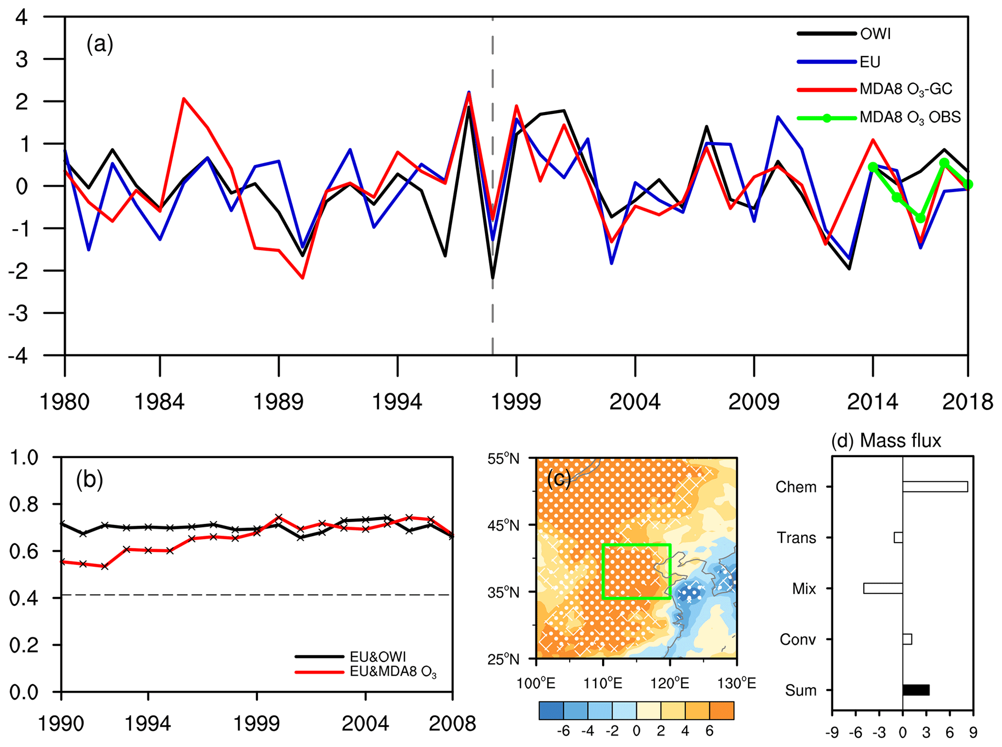
Figure 1(a) The normalized variation in JJA-mean OWI (black), EU index (blue), simulated MDA8 O3 (red) from 1980 to 2018 and observed MDA8 O3 (green) from 2014 to 2018 after detrending. (b) The 21-year sliding correlation coefficients between simulated MDA8 O3 (red), OWI (black) and EU. The black dotted line (crosses) indicates (exceeded) the 95 % confidence level. (c) Composite difference of the simulated MDA8 O3 (unit: µg m−3) in summer between the six highest and the six lowest EU index years from 1980 to 2018. The white dots (hatching) indicate that the difference was above the 95 % (90 %) confidence level (t test). The green box represents the location of North China. (d) Composite difference of the mass fluxes of summer ozone (unit: t d−1) from GEOS-Chem between the six highest and the six lowest EU years from 1980 to 2018. The left axis gives the names of the physicochemical processes: chemical reaction (Chem), transport (Trans), PBL mixing (Mix), convection (Conv) and their sum (Sum).
As mentioned before, the positive phase of the EU pattern was found to have a close relationship with the interannual variations in OWI (Yin et al., 2019); the correlation coefficient was 0.65 from 1980 to 2018 after detrending (Fig. 1a). In the 13 years when OWI reached extreme values (i.e., × standard deviation), the EU pattern also showed large values (i.e., × standard deviation) in 8 years, accounting for 62 % of the larger OWI anomalies. The correlation coefficient between the EU index and simulated MDA8 O3 (i.e., 0.56) also exceeded the 99 % confidence level during 1980–2018. In the EXEU experiment, the simulated MDA8 O3 values in the 6 years with the highest and the 6 years with the lowest EU indexes were composited (highest minus lowest). Because emissions were fixed, the significantly positive anomalies of MDA8 O3 in Fig. 1c resulted from different phases of the EU teleconnection and verified the impacts of the EU pattern on O3 pollution in North China. The physicochemical processes of ozone production in GEOS-Chem simulations were analyzed. When the EU pattern was at a high positive phase, chemical reactions had large positive values. Although transport and mixing had negative values, the sum of all physicochemical processes was 8.27 t d−1, resulting in more O3 (Fig. 1d). Furthermore, the 21-year running correlation coefficient between the EU index and observed OWI (simulated MDA8 O3) remained at approximately 0.7 (0.6) and was persistently above the 99 % confidence level (Fig. 1b), indicating that the connections between the EU pattern and O3-related meteorology in North China did not change over time.
The 39-year correlation coefficients between AM-mean Eurasia snow cover and summer-mean OWI were weakly negative (figure not shown). However, they were significantly negative in West Siberia and central Siberia during 1980–1998 (P1, Fig. 2a) and these correlations disappeared during the period of 1999–2018 (P2, Fig. 2b). The availability of snow data in three regions (i.e., West Siberia, central Siberia and the northern area to Baikal) was verified before confirming the key region of snow cover anomalies. Judging from the spatial and temporal correlation analysis, the reanalysis data of snow cover provided by Rutgers University agreed well with the site observations in West Siberia (62–66∘ N, 75–92∘ E) from 1980 to 2012 (Fig. S5). Thus, the regional mean of AM-mean Eurasian snow cover in this region was defined as SCWS, which was also significantly and negatively correlated with the summer EU pattern (Fig. S6). Furthermore, as pointed out by Yin et al. (2020a), sea ice anomalies in the Gakkel Ridge (SIGR, 82–88∘ N, 0–80∘ E, Fig. S1) also bridged the summer EU and OWI.
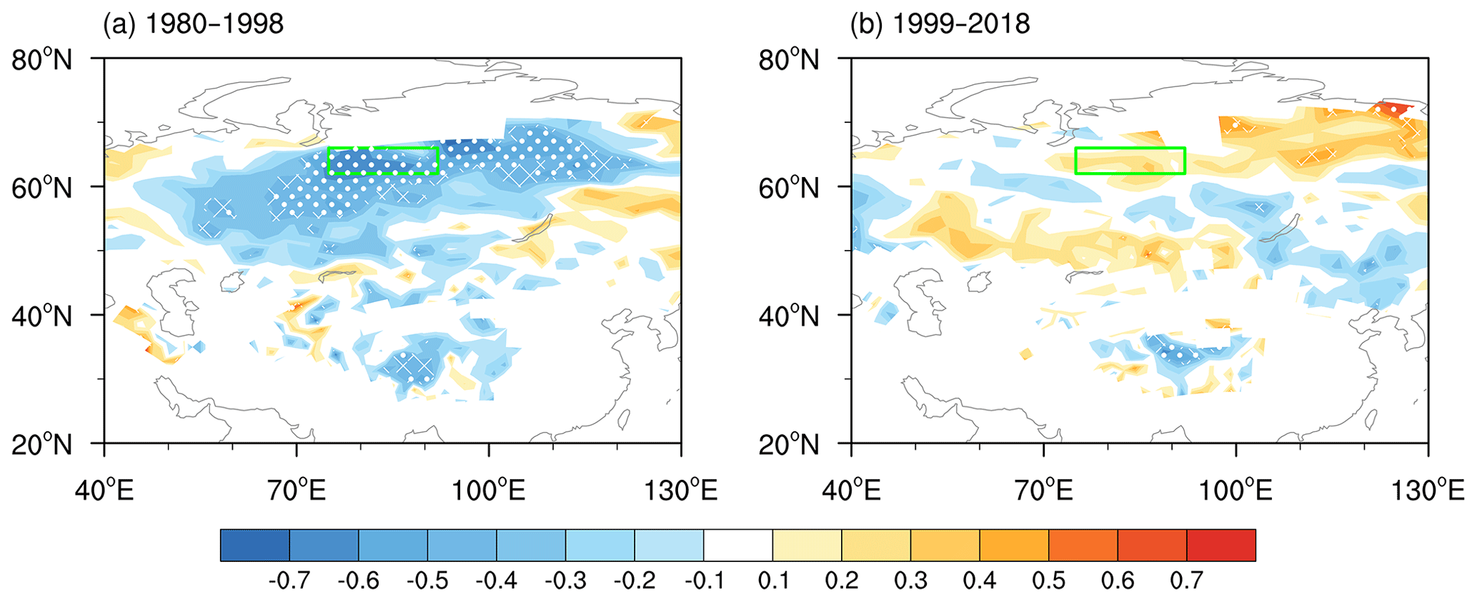
Figure 2The correlation coefficients between the JJA-mean OWI and AM-mean snow cover (a) from 1980 to 1998 and (b) from 1999 to 2018. The white dots (hatching) indicate that the correlation coefficients exceeded the 95 % (90 %) confidence level (t test). The green box represents the key area used to calculate SCWS index. The linear trend is removed.
During 1980–2018, the correlation coefficients between OWI and the above two external forcings were 0.5 (SIGR, significant at the 99 % confidence level) and −0.21 (SCWS, insignificant at the 95 % confidence level), respectively (Fig. 3a, b). We also checked the 21-year running correlation coefficients between each forcing and OWI in Fig. 3c–d, both of which showed decadal changes and independent with the choice of running time window (figure not shown). The correlation between OWI and SCWS was significant (−0.68, above the 99 % confidence level) during P1 and became insignificant (0.20) during P2 (Fig. 3c). Oppositely, the correlation with SIGR enhanced from 0.4 in P1 to 0.62 in P2 (Fig. 3d). After removing the signal of El Niño–Southern Oscillation (ENSO), these correlation coefficients were almost unchanged. Interestingly, the connections between these two preceding factors and the EU pattern illustrated similar decadal changes (Fig. 3c, d). That is, the correlation between EU and SCWS was only significant (−0.62) in the former period; however, the correlation between EU and SIGR was only significant (0.61) after the mid-1990s (Fig. 3c, d). Furthermore, SIGR and SCWS were mutually independent, because the 21-year running correlation coefficient between them was maintained at a low level (Fig. S7). Therefore, we speculated that the impacts of the summer EU pattern on ground-level O3 pollution in North China were robust and long-standing (Fig. 1b). However, the preceding factors inducing the EU pattern to influence the O3 pollution in North China changed from SCWS in P1 to SIGR in P2 (Fig. 3c, d).
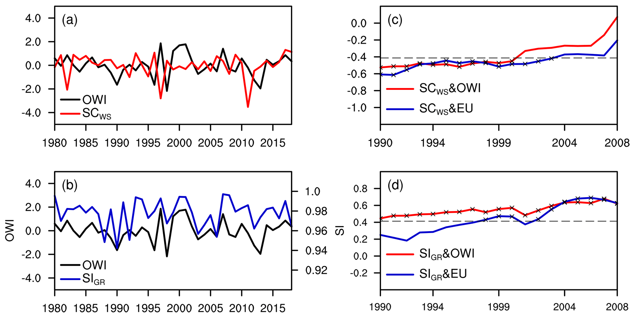
Figure 3The normalized variation in (a) OWI (black) and SCWS (red), (b) OWI (black) and SIGR (blue) from 1980 to 2018 after detrending. The 21-year sliding correlation coefficients between (c) SCWS and OWI (red) and SCWS and EU (blue), as well as (d) SIGR and OWI (red) and SIGR and EU (blue). The black dotted line (crosses) indicates (exceeded) the 95 % confidence level. The linear trend is removed.
The physical mechanism of how to achieve the impacts of SCWS on surface O3 pollution in North China is still a new question to the best of our knowledge. As an efficient climate forcing, the snow cover anomalies could stimulate synchronous responses in the atmosphere by changing albedo and hydrological effects and could then impact the atmosphere in the following seasons (Cohen and Rind, 1991). In April and May, the snow at high latitudes began to melt and had obvious interannual variations, as shown by both the observations and the reanalysis data (Fig. S5). Generally, lower albedo, associated with less snow cover, meant that the land–snow surface reflected less solar radiation and resulted in higher SAT. Warmer surfaces produce stronger longwave radiation and heat the local atmosphere from the surface to the mid-troposphere (Chen et al., 2003, 2016). Moreover, the changing local soil moisture enhanced the surface heat flux and thus resulted in higher SAT and atmospheric temperatures (Zhang et al., 2017). Finally, the warmed thermal conditions in the atmosphere enhanced the local 1000–500 hPa thickness and represented positive anomalies of Z500 (Chen et al., 2003; Halder and Dirmeyer, 2017). Compared to P1, the southern edge of the area with high concentrations of snow (>85 %) in late spring shifted northward by approximately 2∘ in latitude during P2 (Fig. 4a). Similarly, the significant changes in radiation flux (shortwave + longwave) and heat flux (latent + sensible) also moved northward in P2 relative to P1 (Fig. 4b, c). We speculated that this northward movement of effective snow cover, accompanied by shifts in net heat flux, possibly contributed to the changing relationship between SCWS and OWI.
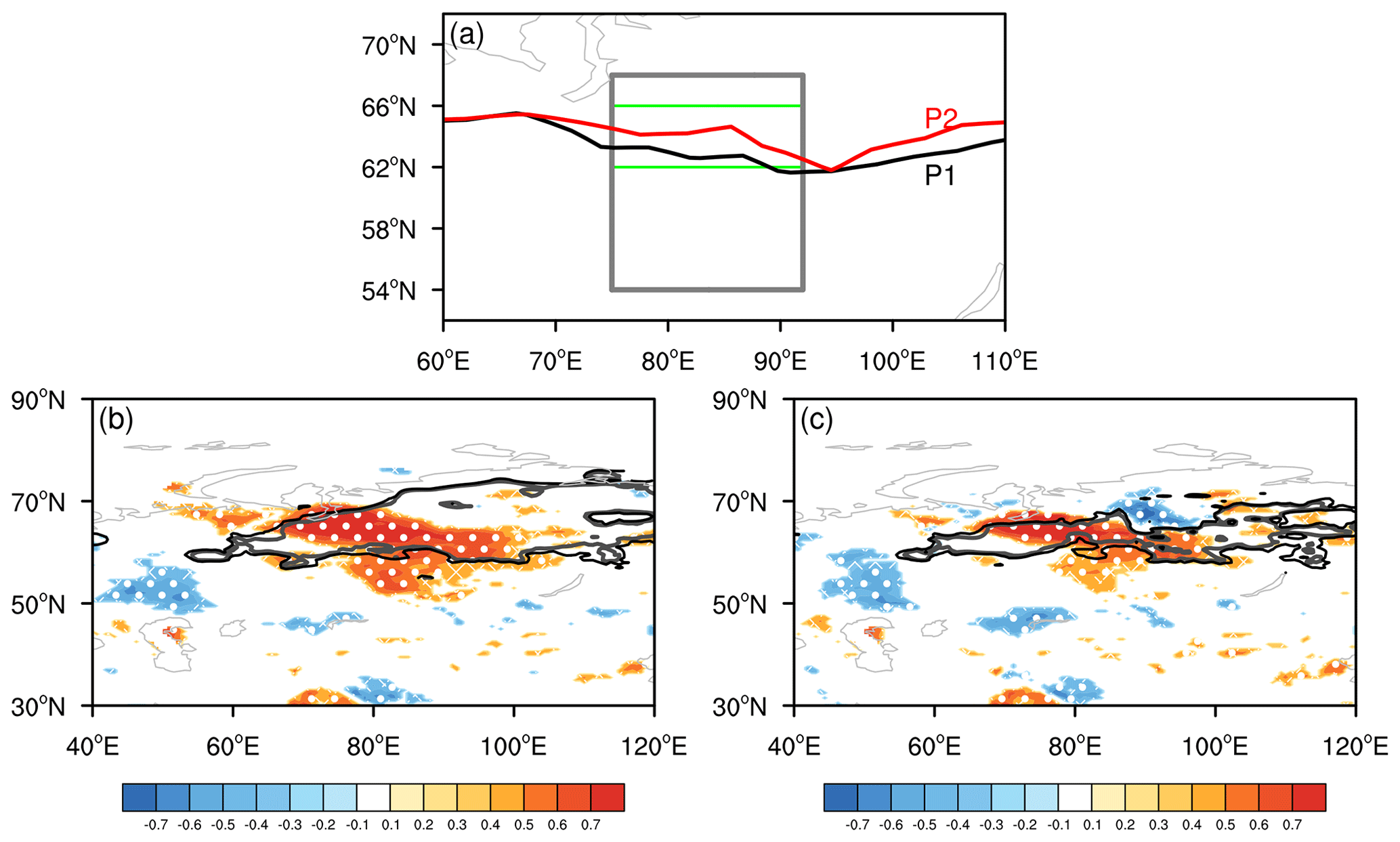
Figure 4(a) The southern edge of the 85 % snow cover concentration during 1980–1993 (black) and during 2004–2018 (red). The gray (green) box represents the key area used to calculate NHFWS (SCWS) index. The correlation coefficients between SCWS × −1 and (b) surface net radiation flux (shortwave + longwave) and (c) surface net heat flux (latent + sensible) are displayed during 1980–1998 (shading) and 1999–2018 (contour). White dots (hatching) indicate the correlation coefficients during P1, exceeding the 95 % (90 %) confidence level (t test). The gray (black) contours represent the correlation coefficients during P2, exceeding the 95 % (90 %) confidence level. The linear trend is removed.
The local responses of geopotential height in the mid-troposphere induced by negative anomalies of SCWS illustrated decadal changes; that is, the significant correlation coefficients between SCWS × −1 and Z500, as well as SAT, were distributed more southward and were stronger in P1 (Fig. 5a) than in P2 (Fig. 5c). For convenience, the roles of radiation and heat flux (shortwave + longwave + latent + sensible) were considered together as net heat flux (Zhang et al., 2017), which was averaged over West Siberia (54–68∘ N, 75–92∘ E) and defined as NHFWS. It was evident that the atmospheric responses associated with NHFWS agreed well with those of less SCWS (Fig. 5b, d). That is, the enhanced net heat flux related to decreased snow cover in West Siberia heated the above atmosphere and resulted in local warmer SAT and anticyclonic circulations in the mid-troposphere during P1 (Fig. 5a, b). In addition, cyclonic responses can be found on the left and right sides of the aforementioned anticyclonic anomalies in April–May (Fig. 5a, b). However, similar to the radiation and heat flux in Fig. 4b–c, the atmospheric responses were distributed more northward and were weaker during P2 than during P1 (Fig. 5c, d).
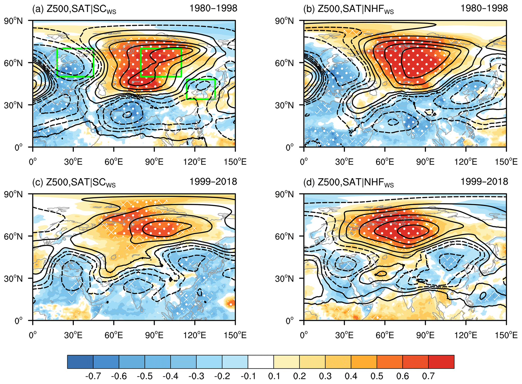
Figure 5The correlation coefficients between SCWS × −1 (a, c), NHFWS (b, d) and surface air temperature (shading) and geopotential height at 500 hPa (contour) from 1980 to 1998 (a, b) and from 1999 to 2018 (c, d). The white dots (hatching) indicate that the correlation coefficients (in shading) exceeded the 95 % (90 %) confidence level (t test). The green boxes represent the anomalous cyclonic or anticyclonic centers in AM. The linear trend is removed.
The AM-mean NHFWS showed significantly positive correlations with both the summer-mean EU (0.49) and OWI (0.52) during P1 (Figs. 6a, S8a). After removing the ENSO signal, these correlated relationships almost showed no difference. Furthermore, the “” anomalous atmospheric centers in April–May (green boxes in Fig. 5a) had significantly positive correlations with the summer EU pattern (CC = 0.45, above the 95 % confidence level). The atmospheric anomalies stimulated by negative SCWS could appear as positive phases of the EU pattern in JJA during P1 (Figs. 6b, S8a). As one center of the EU pattern, the anticyclonic anomalies over North China were significant in the mid and lower troposphere (Figs. 6b, 7a) and resulted in clear skies (Fig. 7c). Sinking heating, intense sunlight (Fig. 7c) and less precipitation (correspondingly more cloud and weaker ultraviolet radiations, Fig. 7a) resulted in beneficial environments for the natural emissions of O3 precursors (Lu et al., 2019) and photochemical reactions (Pu et al., 2017). Differently, the northward and weaker atmospheric responses in April–May were almost dispersed in summer (Figs. 6c, S8b) and had only slight impacts on the local OWI in North China (Fig. 7b, d) during P2, which were consistent with the insignificant correlations between NHFWS and the EU (OWI) (Fig. 6a).
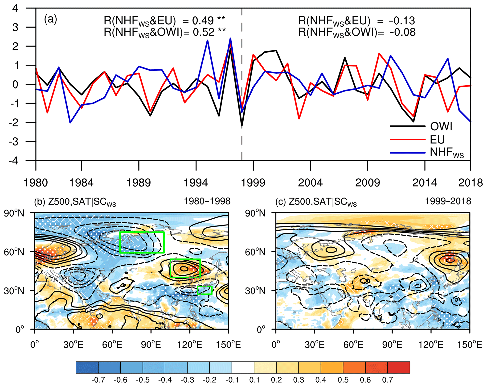
Figure 6(a) The normalized variation in the JJA OWI (black), JJA EU index (red) and AM NHFWS (blue) from 1980 to 2018 after detrending. The numbers represent the correlation coefficients between NHFWS and EU and between NHFWS and OWI during 1980–1998 and 1999–2018, respectively. Two asterisks indicate that the correlation coefficients exceeded the 95 % confidence level. The correlation coefficients between SCWS × −1 and JJA surface air temperature (shading) and geopotential height at 500 hPa (contour) from 1980 to 1998 (b) and from 1999 to 2018 (c) are shown. The white dots (hatching) indicate that the correlation coefficients with surface air temperature exceeded the 95 % (90 %) confidence level (t test). The green boxes represent the key areas used to calculate the EU index. The linear trend is removed.
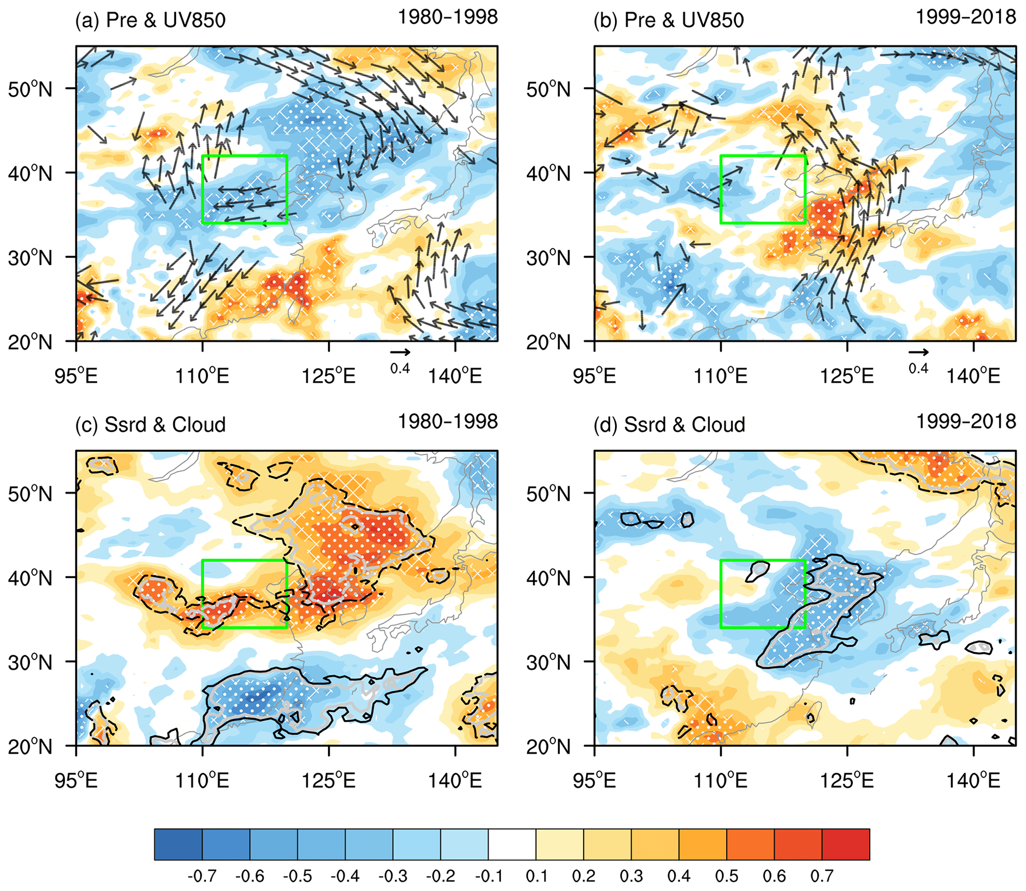
Figure 7The meteorological conditions associated with SCWS × −1. (a, b) The correlation coefficients between SCWS × −1 and precipitation (shading) and wind at 850 hPa (arrow); (c, d) surface incoming shortwave flux (shading) and the sum of low and medium cloud cover (contour) from 1980 to 1998 (a, c) and from 1999 to 2018 (b, d). The white dots (hatching) indicate that the correlation coefficients represented with shading exceeded the 95 % (90 %) confidence level (t test). The gray (black) contours exceeded the 95 % (90 %) confidence level. The green boxes represent the location of North China. The linear trend is removed.
In the EXSC experiment, the simulated MDA8 O3 and mass fluxes of ozone were composited (three lowest SCWS minus highest) during P1 and P2, respectively. During P1, the composited results (with fixed emissions) were significantly positive (Fig. 8a) and were in good agreement with the proposed mechanisms (i.e., less snow cover in West Siberia resulted in severe surface O3 pollution in North China). The responses of MDA8 O3 pollution in North China were insignificant during P2 (Fig. 8b) and were also consistent with both weak impacts in this period and changing relationships. Mass balance of ozone is jointly determined by four processes (i.e., chemistry, transport, PBL mixing and convection) which could be isolated by the GEOS-Chem model. During P1, the composite results of chemical reaction had large positive values (11.05 t d−1) (Fig. 8a), indicating that the dry, hot meteorological conditions were conductive to produce more O3. Anomalous anticyclonic circulations located above the North China region resulted in downward air flow that may bring ozone from the stratosphere to the surface. Hence, the value of convection was also positive. The values of transport and mixing were negative (Fig. 8a), but the sum of all processes was positive, indicating that the ozone concentrations in North China would increase. However, the composite results of chemical, transport and mixing were opposite (Fig. 8b) during P2 compared with P1. Meanwhile, the values of convection and the sum were extremely close to zero (Fig. 8b), indicating that there were only slight impacts on ozone in North China when SCWS was low during P2. The composite results of mass fluxes were well in agreement with the previous conclusion.
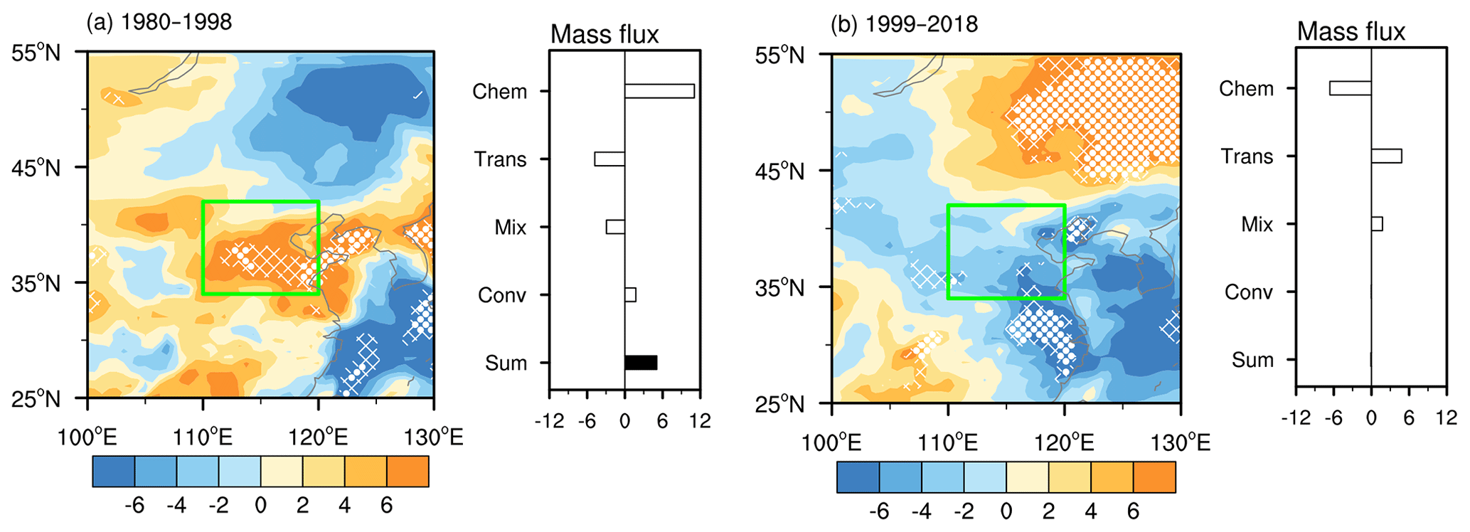
Figure 8Composite difference of the summer MDA8 O3 (unit: µg m−3) simulated by the GEOS-Chem model between the three lowest and the three highest SCWS years (a) from 1980 to 1998 and (b) from 1999 to 2018. The white dots (hatching) indicate that the difference was above the 95 % (90 %) confidence level (t test). The green boxes represent the location of North China. The bar chart on the right is the composite difference of the summer mass fluxes of ozone (unit: t d−1) during each periods. The left axis gives the names of the physicochemical processes: chemical reaction (Chem), transport (Trans), PBL mixing (Mix), convection (Conv) and their sum (Sum). The results were calculated within the planetary boundary layer.
In this study, the April–May snow cover in West Siberia was newly proposed as a preceding climate driver that influenced the surface O3-related meteorology in North China during 1980–1998, and the associated physical mechanisms were also explained by comparing the periods before and after the mid-1990s. Accompanying the northward shift of dense snow cover, the associated radiation and heat flux also retreated toward the polar region during 1999–2018 (Fig. 4); thus, the induced atmospheric anomalies were located northward in April–May and disappeared in summer (Fig. 5c, d). However, in the period of 1980–1998, the positive phase of the EU pattern in summer could be stimulated by negative anomalies of snow cover (mainly by enhanced net heat flux) in West Siberia (Fig. 6). Consequently, hot, dry air and intense solar radiation under anomalous anticyclonic circulations not only enhanced the natural emissions of O3 precursors but also promoted photochemical reactions to produce more O3 near the surface (Figs. 7, 8). To enhance the robustness of this study, the ERA5 reanalysis data were also employed to reproduce the observational analyses. As shown in Fig. S9, identical results were obtained and confirmed.
The linkage between the EU pattern and MDA8 O3 was robust, which bridged SCWS and OWI in the period of 1980–1998 but connected the SIGR and OWI after the mid-1990s. In Fig. 9, OWI data were regressed by SCWS and SIGR from 1980–2018. The 21-year running correlation coefficient between OWI and the fitted values stably maintained around 0.6 and indicated that these two preceding factors almost introduced the full impacts of the EU pattern (Fig. 1b) over the whole period. Generally, the decadal changes in the climate drivers influence the stability of the predictability. It is evident that our results overcame this problem and deepened the understanding of variations in summer O3 from the climate perspective. Yin et al. (2020a) also found that the sea ice anomalies over the Canada Basin and the Beaufort Sea (Fig. S1) also stimulated a Rossby-wave-like train propagating through the North Pacific to influence the variability in OWI in North China. When we added these sea ice anomalies into the regressions, the fitting performance was visibly improved, because the 21-year running correlation coefficient was elevated to approximately 0.8 with OWI, as seen in Fig. 9b.
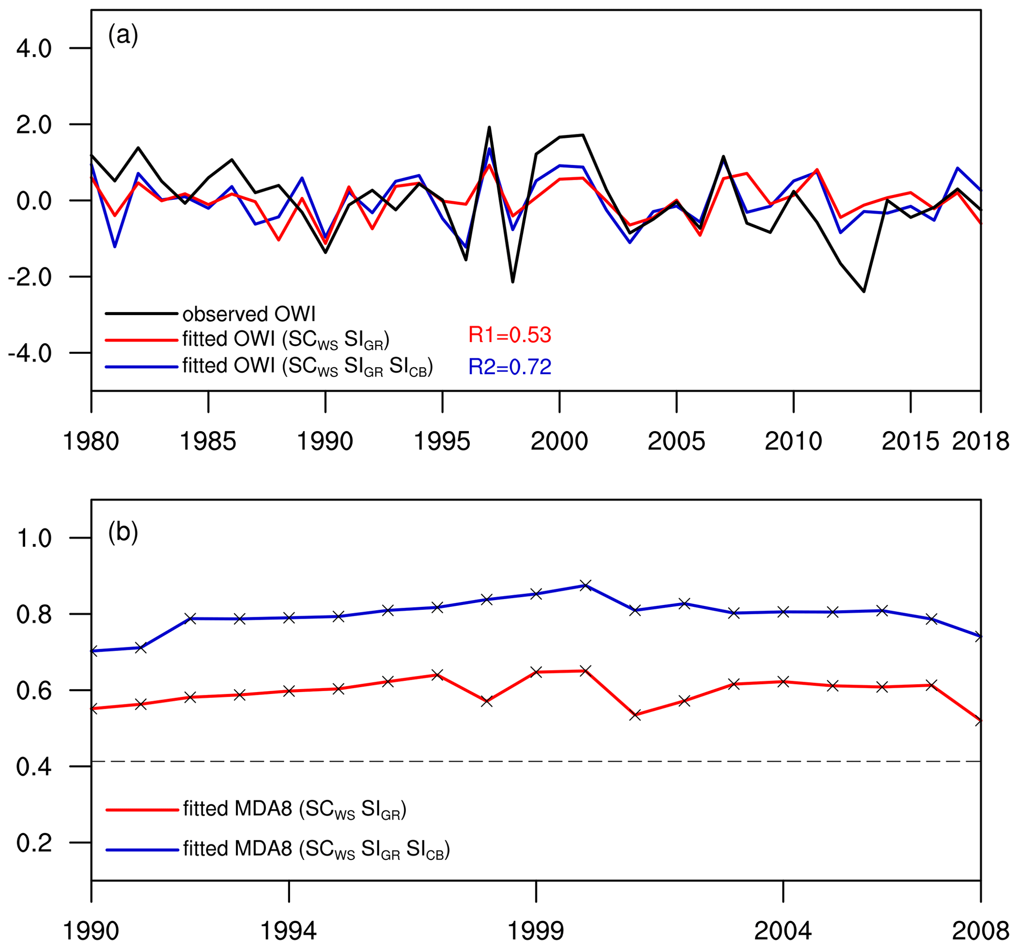
Figure 9(a) The variation in the JJA-mean observed OWI (black), the fitted OWI-1 (by SCWS and SIGR, red) and the fitted OWI-2 (by SCWS, SIGR and SICB, blue) from 1980 to 2018 after detrending. (b) The 21-year sliding correlation coefficients between observed OWI and fitted OWI-1 (red) or fitted OWI-2 (blue). The black dotted line (crosses) indicates (exceeded) the 95 % confidence level.
The concentrations of surface O3 have been extensively measured since 2014 in China; this timescale cannot support the study of the interannual–decadal variability in O3 pollution. In this study, we used two datasets, i.e., the ozone weather index and the O3 concentrations simulated by GEOS-Chem, to focus on the impacts of climate variability on surface O3 in North China. Although the feasibility of these datasets was strictly examined, there were still gaps between the real variations in O3 and the variations in these two substitutions; this discrepancy requires further research. Moreover, the climate–chemistry coupled model needs to be used to verify the role of snow cover on ozone pollution in North China in further studies. Furthermore, there is no doubt that anthropogenic emissions are the fundamental drivers of O3 pollution, which has been investigated in many previous studies (N. Li et al., 2018; K. Li et al., 2019; Dang et al., 2020). After removal of the linear trend, the signals of climate warming in the atmosphere were also eliminated, which allowed us to focus on the interannual variations. In addition, the decrease in haze aerosols was also proven to be an effective contributor to recent interannual variations in O3 concentrations (K. Li et al., 2019), which were not involved in our study and need further attention.
Hourly O3 concentration data can be downloaded from https://quotsoft.net/air/ (Ministry of Environmental Protection of China, 2021). Sea ice concentration data are from https://www.metoffice.gov.uk/hadobs/hadisst/data/download.html (Met Office Hadley Centre, 2020). Snow cover data can be downloaded from Rutgers University at http://climate.rutgers.edu/snowcover/ (Rutgers University, 2021). The observed snow data from meteorological stations are available at http://meteo.ru/data/165-snow-cover (Russian Federal Service For Hydrometeorology and Environmental Monitoring, 2021). The monthly-mean MERRA2 reanalysis datasets are available at https://disc.gsfc.nasa.gov/datasets?page=1 (MERRA2, 2021). The monthly-mean ERA5 reanalysis datasets are available at https://cds.climate.copernicus.eu/cdsapp#!/home (Copernicus Climate Change Service, 2021).
The supplement related to this article is available online at: https://doi.org/10.5194/acp-21-11519-2021-supplement.
HW and ZY designed and performed the research. YW did the statistical analysis and implemented the GEOS-Chem simulations. ZY prepared the article with contributions from all co-authors.
The authors declare that they have no conflict of interest.
Publisher’s note: Copernicus Publications remains neutral with regard to jurisdictional claims in published maps and institutional affiliations.
This research was supported by National Natural Science Foundation of China (91744311, 42088101, 41991283 and 42025502).
This research has been supported by the National Natural Science Foundation of China (grant nos. 91744311, 42088101, 41991283 and 42025502).
This paper was edited by Qiang Zhang and reviewed by two anonymous referees.
Bey, I., Jacob, D. J., Yantosca, R. M., Logan, J. A., Field, B., Fiore, A. M., Li, Q., Liu, H., Mickley, L. J., and Schultz, M.: Global modeling of tropospheric chemistry with assimilated meteorology: Model description and evaluation, J. Geophys. Res., 106, 23073–23095, https://doi.org/10.1029/2001JD000807, 2001.
Bulygina, O. N., Groisman, P. Y., Razuvaev, V. N., and Korshunova, N. N.: Changes in snow cover characteristics over Northern Eurasia since 1966, Environ. Res. Lett., 6, 045204, https://doi.org/10.1088/1748-9326/6/4/045204, 2011.
Chen, H. S., Sun, Z. B., and Zhu, W. J.: The Effects of Eurasian Snow Cover Anomaly on Winter Atmospheric General Circulation Part II. Model Simulation, Chinese J. Atmos. Sci., 27, 547–860, https://doi.org/10.3878/j.issn.1006-9895.2003.03.02, 2003 (in Chinese).
Chen, S. F., Wu, R. G., and Liu, Y.: Dominant Modes of Interannual Variability in Eurasian Surface Air Temperature during Boreal Spring, J. Climate, 29, 1109–1125, https://doi.org/10.1175/JCLI-D-15-0524.1, 2016.
Copernicus Climate Change Service: ERA5: fifth generation of ECMWF atmospheric reanalyses of the global climate Copernicus Climate Change Service Climate Data Store, available at: https://cds.climate.copernicus.eu/cdsapp#!/home, last access: 13 July 2021.
Cohen, J. and Rind, D.: The effect of snow cover on the climate, J. Climate, 4, 689–706, https://doi.org/10.1175/1520-0442(1991)004<0689:TEOSCO>2.0.CO;2, 1991.
Dang, R. J., Liao, H., and Fu, Y.: Quantifying the anthropogenic and meteorological influences on summertime surface ozone in China over 2012–2017, Sci. Total Environ., 754, 142394, https://doi.org/10.1016/j.scitotenv.2020.142394, 2020.
Fix, M. J., Cooley, D., Hodzic, A., Gilleland, E., Russell, B. T., Porter, W. C., and Pfister, G. G.: Observed and predicted sensitivities of extreme surface ozone to meteorological drivers in three US cities, Atmos. Environ., 176, 292–300, https://doi.org/10.1016/j.atmosenv.2017.12.036, 2018.
Gelaro, R., McCarty, W., Suarez, M. J., Todling, R., Molod, A., Takacs, L., Randles, C. A., Darmenov, A., Bosilovich, M. G., Reichle, R., Wargan, K., Coy, L., Cullather, R., Draper, C., Akella, S., Buchard, V., Conaty, A., da Silva, A. M., Gu, W., Kim, G. K., Koster, R., Lucchesi, R., Merkova, D., Nielsen, J. E., Partyka, G., Pawson, S., Putman, W., Rienecker, M., Schubert, S. D., Sienkiewicz, M., and Zhao, B.: The Modern-Era Retrospective Analysis for Research and Applications, Version 2 (MERRA2), J. Climate, 30, 5419–5454, https://doi.org/10.1175/JCLI-D-16-0758.1, 2017.
Gong, C. and Liao, H.: A typical weather pattern for ozone pollution events in North China, Atmos. Chem. Phys., 19, 13725–13740, https://doi.org/10.5194/acp-19-13725-2019, 2019.
Gong, C., Liao, H., Zhang, L., Yue, X., Dang, R. J., and Yang, Y.: Persistent ozone pollution episodes in North China exacerbated by regional transport, Environ. Pollut., 265, 115056, https://doi.org/10.1016/j.envpol.2020.115056, 2020.
Gong, D. Y., Wang, S. W., and Zhu, J. H.: East Asian winter monsoon and Arctic oscillation, Geophys. Res. Lett., 28, 2073–2076, https://doi.org/10.1029/2000GL012311, 2001.
Halder, S. and Dirmeyer, P. A.: Relation of Eurasian Snow Cover and Indian Summer Monsoon Rainfall: Importance of the Delayed Hydrological Effect, J. Climate, 30, 1273–1289, https://doi.org/10.1175/JCLI-D-16-0033.1, 2017.
Holtslag, A. and Boville, B. A.: Local versus nonlocal boundary layer diffusion in a global climate model, J. Climate, 6, 1825–1842, https://doi.org/10.1175/1520-0442(1993)006<1825:LVNBLD>2.0.CO;2, 1993.
Li, H., Chen, H., Wang, H., Sun, J., and Ma, J.: Can Barents Sea Ice Decline in Spring Enhance Summer Hot Drought Events over Northeastern China?, J. Climate, 31, 4705–4725, https://doi.org/10.1175/JCLI-D-17-0429.1, 2018.
Li, K., Jacob, D. J., Liao, H., Shen, L., Zhang, Q., and Bates, K. H.: Anthropogenic drivers of 2013-2017 trends in summer surface ozone in China, P. Natl. Acad. Sci. USA, 116, 422–427, https://doi.org/10.1073/pnas.1812168116, 2019.
Li, M., Zhang, Q., Kurokawa, J.-I., Woo, J.-H., He, K., Lu, Z., Ohara, T., Song, Y., Streets, D. G., Carmichael, G. R., Cheng, Y., Hong, C., Huo, H., Jiang, X., Kang, S., Liu, F., Su, H., and Zheng, B.: MIX: a mosaic Asian anthropogenic emission inventory under the international collaboration framework of the MICS-Asia and HTAP, Atmos. Chem. Phys., 17, 935–963, https://doi.org/10.5194/acp-17-935-2017, 2017.
Li, N., He, Q., Greenberg, J., Guenther, A., Li, J., Cao, J., Wang, J., Liao, H., Wang, Q., and Zhang, Q.: Impacts of biogenic and anthropogenic emissions on summertime ozone formation in the Guanzhong Basin, China, Atmos. Chem. Phys., 18, 7489–7507, https://doi.org/10.5194/acp-18-7489-2018, 2018.
Li, Y., Sheng, L., Li, C., and Wang, Y.: Impact of the Eurasian Teleconnection on the Interannual Variability of Haze-Fog in Northern China in January, Atmosphere, 10, 113, https://doi.org/10.3390/atmos10030113, 2019.
Liao, H., Chen, W. T., and Seinfeld, J. H.: Role of climate change in global predictions of future tropospheric ozone and aerosols, J. Geophys. Res.-Atmos., 111, D12304, https://doi.org/10.1029/2005JD006852, 2006.
Lim, Y. K. and Kim, H. D.: Comparison of the impact of the Arctic Oscillation and Eurasian teleconnection on interannual variation in East Asian winter temperatures and monsoon, Theor. Appl. Climatol., 124, 267–279, https://doi.org/10.1007/s00704-015-1418-x, 2016.
Liu, Y. and Chen, W.: Variability of the Eurasian teleconnection pattern in the Northern Hemisphere winter and its influences on the climate in China, Chinese J. Atmos. Sci., 36, 423–432, https://doi.org/10.2151/jmsj1965.77.2_495, 2012 (in Chinese).
Liu, Y., Wang, L., Zhou, W., and Chen, W.: Three Eurasian teleconnection patterns: spatial structures, temporal variability, and associated winter climate anomalies, Clim. Dynam., 42, 2817–2839, https://doi.org/10.1007/s00382-014-2163-z, 2014.
Lu, X., Zhang, L., Chen, Y. F., Zhou, M., Zheng, B., Li, K., Liu, Y. M., Lin, J. T., Fu, T. M., and Zhang, Q.: Exploring 2016–2017 surface ozone pollution over China: source contributions and meteorological influences, Atmos. Chem. Phys., 19, 8339–8361, https://doi.org/10.5194/acp-19-8339-2019, 2019.
MERRA2: meteorological data, available at: https://disc.gsfc.nasa.gov/datasets?page=1, last access: 21 March 2021.
Met Office Hadley Centre: Sea ice concentration data, available at: https://www.metoffice.gov.uk/hadobs/hadisst/data/download.html, last access: 8 December 2020.
Ministry of Environmental Protection of China: Hourly O3 concentration data, available at: https://quotsoft.net/air/, last access: 18 July 2021.
Pu, X., Wang, T., Huang, X., Melas, D., Zanis, P., Papanastasiou, D., and Poupkou, A.: Enhanced surface ozone during the heat wave of 2013 in Yangtze River delta region, China, Sci. Total Environ., 603, 807–816, https://doi.org/10.1016/j.scitotenv.2017.03.056, 2017.
Rayner, N., Parker, D. E., Horton, E., Folland, C., Alexander, L., Rowell, D., Kent, E., and Kaplan, A.: Global analyses of sea surface temperature, sea ice, and night marine air temperature since the late nineteenth century, J. Geophys. Res.-Atmos., 108, 4407, https://doi.org/10.1029/2002JD002670, 2003.
Robinson, D. A., Dewey, K. F., and Heim, R. R.: Global snow cover monitoring: an update, B. Am. Meteorol. Soc., 74, 1689–1696, https://doi.org/10.1175/1520-0477(1993)074<1689:GSCMAU>2.0.CO;2, 1993.
Russian Federal Service For Hydrometeorology and Environmental Monitoring (ROSHYDROMET): observed station snow cover data, available at: http://meteo.ru/data/165-snow-cover, last access: 22 July 2021.
Rutgers University: Snow cover data, available at: http://climate.rutgers.edu/snowcover/, last access: 19 July 2021.
Wallace, J. M. and Gutzler, D. S.: Teleconnections in the geopotential height field during the Northern Hemisphere winter, Mon. Weather Rev., 109, 784–812, https://doi.org/10.1175/1520-0493(1981)109<0784:TITGHF>2.0.CO;2, 1981.
Wang, H. J. and He, S. P.: The North China/Northeastern Asia Severe Summer Drought in 2014, J. Climate, 28, 6667–6681, https://doi.org/10.1175/JCLI-D-15-0202.1, 2015.
Wang, N. and Zhang, Y. C.: Evolution of Eurasian teleconnection pattern and its relationship to climate anomalies in China, Clim. Dynam., 44, 1017–1028, https://doi.org/10.1007/s00382-014-2171-z, 2015.
Wei, J., Zhang, Q. Y., and Tao, S. Y.: Physical causes of the 1999 and 2000 summer severe drought in North China, Chinese J. Atmos. Sci., 28, 125–137, https://doi.org/10.1091/mbc.7.4.565, 2004 (in Chinese).
Wu, B., Zhang, R., Wang, B., and D'Arrigo, R.: On the association between spring Arctic sea ice concentration and Chinese summer rainfall, Geophys. Res. Lett., 36, L09501, https://doi.org/10.1029/2009GL037299, 2009.
Yan, H., Duan, W., and Xiao, Z.: A study on relation between East Asian winter monsoon and climate change during raining season in China, J. Trop. Meteor., 19, 367–376, https://doi.org/10.3969/j.issn.1006-8775.2004.01.003, 2003.
Yim, S. Y., Jhun, J. G., Lu, R., and Wang, B.: Two distinct patterns of spring Eurasian snow cover anomaly and their impacts on the East Asian summer monsoon, J. Geophys. Res.-Atmos., 115, D22113, https://doi.org/10.1029/2010JD013996, 2010.
Yin, Z., Wang, H., Li, Y., Ma, X., and Zhang, X.: Links of climate variability in Arctic sea ice, Eurasian teleconnection pattern and summer surface ozone pollution in North China, Atmos. Chem. Phys., 19, 3857–3871, https://doi.org/10.5194/acp-19-3857-2019, 2019.
Yin, Z. C., Yuan, D. M., Zhang, X. Y., Yang, Q., and Xia, S. W.: Different contributions of Arctic sea ice anomalies from different regions to North China summer ozone pollution, Int. J. Climatol., 40, 559–571, https://doi.org/10.1002/joc.6228, 2020a.
Yin, Z. C., Li, Y. Y., and Cao, B. F.: Seasonal Prediction of Surface O3-related Meteorological Conditions in summer in North China, Atmos. Res., 246, 105–110, https://doi.org/10.1016/j.atmosres.2020.105110, 2020b.
Zhang, R. N., Sun, C. H., and Li, W. J.: Relationship between the interannual variations of Arctic sea ice and summer Eurasian teleconnection and associated influence on summer precipitation over China, Chinese J. Geophys., 61, 91–105, https://doi.org/10.6038/cjg2018K0755, 2018 (in Chinese).
Zhang, R. N., Zhang, R. H., and Zuo, Z. Y.: Impact of Eurasian Spring Snow Decrement on East Asian Summer Precipitation, J. Climate, 30, 3421–3437, https://doi.org/10.1175/JCLI-D-16-0214.1, 2017.
Zheng, B., Tong, D., Li, M., Liu, F., Hong, C., Geng, G., Li, H., Li, X., Peng, L., Qi, J., Yan, L., Zhang, Y., Zhao, H., Zheng, Y., He, K., and Zhang, Q.: Trends in China's anthropogenic emissions since 2010 as the consequence of clean air actions, Atmos. Chem. Phys., 18, 14095–14111, https://doi.org/10.5194/acp-18-14095-2018, 2018.