the Creative Commons Attribution 4.0 License.
the Creative Commons Attribution 4.0 License.
 | 09 Jul 2021
Orographically induced spontaneous imbalance within the jet causing a large-scale gravity wave event
Markus Geldenhuys
Peter Preusse
Isabell Krisch
Christoph Zülicke
Jörn Ungermann
Manfred Ern
Felix Friedl-Vallon
Martin Riese
To better understand the impact of gravity waves (GWs) on the middle atmosphere in the current and future climate, it is essential to understand their excitation mechanisms and to quantify their basic properties. Here a new process for GW excitation by orography–jet interaction is discussed. In a case study, we identify the source of a GW observed over Greenland on 10 March 2016 during the POLSTRACC (POLar STRAtosphere in a Changing Climate) aircraft campaign. Measurements were taken with the Gimballed Limb Observer for Radiance Imaging of the Atmosphere (GLORIA) instrument deployed on the High Altitude Long Range (HALO) German research aircraft. The measured infrared limb radiances are converted into a 3D observational temperature field through the use of inverse modelling and limited-angle tomography. We observe GWs along a transect through Greenland where the GW packet covers ≈ of the Greenland mainland. GLORIA observations indicate GWs between 10 and 13 km of altitude with a horizontal wavelength of 330 km, a vertical wavelength of 2 km and a large temperature amplitude of 4.5 K. Slanted phase fronts indicate intrinsic propagation against the wind, while the ground-based propagation is with the wind. The GWs are arrested below a critical layer above the tropospheric jet. Compared to its intrinsic horizontal group velocity (25–72 m s−1) the GW packet has a slow vertical group velocity of 0.05–0.2 m s−1. This causes the GW packet to propagate long distances while spreading over a large area and remaining constrained to a narrow vertical layer. A plausible source is not only orography, but also out-of-balance winds in a jet exit region and wind shear. To identify the GW source, 3D GLORIA observations are combined with a gravity wave ray tracer, ERA5 reanalysis and high-resolution numerical experiments. In a numerical experiment with a smoothed orography, GW activity is quite weak, indicating that the GWs in the realistic orography experiment are due to orography. However, analysis shows that these GWs are not mountain waves. A favourable area for spontaneous GW emission is identified in the jet by the cross-stream ageostrophic wind, which indicates when the flow is out of geostrophic balance. Backwards ray-tracing experiments trace into the jet and regions where the Coriolis and the pressure gradient forces are out of balance. The difference between the full and a smooth-orography experiment is investigated to reveal the missing connection between orography and the out-of-balance jet. We find that this is flow over a broad area of elevated terrain which causes compression of air above Greenland. The orography modifies the wind flow over large horizontal and vertical scales, resulting in out-of-balance geostrophic components. The out-of-balance jet then excites GWs in order to bring the flow back into balance. This is the first observational evidence of GW generation by such an orography–jet mechanism.
- Article
(13443 KB) - Full-text XML
- BibTeX
- EndNote


Gravity waves (GWs) are ever-present in the Earth's atmosphere. Gravity waves are emitted in the troposphere by flow over orography (e.g. Bacmeister et al., 1994; Eckermann and Preusse, 1999; Durran, 2003; Geldenhuys et al., 2019), by convection (Pfister et al., 1993; Alexander and Pfister, 1995; Chun and Baik, 1998; McLandress et al., 2000; Beres et al., 2004; Choi et al., 2012; Trinh et al., 2016) and by fronts (Snyder et al., 1993; Ralph et al., 1999; Charron and Manzini, 2002). Other sources, such as an out-of-balance jet (O'Sullivan and Dunkerton, 1995; Zülicke and Peters, 2006; Plougonven and Zhang, 2014), vertical wind shear (Lott, 1997) and a planetary-wave-induced critical layer in the polar vortex (Polichtchouk and Scott, 2020), occur in both the troposphere and middle atmosphere. The excitation of GWs from an out-of-balance jet by a geostrophic adjustment frequently occurs during strong Rossby wave activity (Zülicke and Peters, 2006; Plougonven and Zhang, 2014; Ern et al., 2016). Secondary wave generation from breaking GWs (Vadas and Fritts, 2002; Vadas and Becker, 2019; Heale et al., 2020) is another possible source of GWs throughout the atmosphere.
Gravity waves can impact our lives directly through the generation of turbulence, endangering air traffic (Fritts and Alexander, 2003; Bramberger et al., 2018; Geldenhuys et al., 2019). Additionally, they are known to enhance and act as a trigger for convection (de la Torre et al., 2011), impact the movement of weather systems and affect the ozone hole (Kidston et al., 2015). Gravity waves are essential drivers of the middle atmosphere circulation (Holton, 2004) through drag deposited by their breaking and saturation (McLandress, 1998; Alexander et al., 2010). By downward coupling, these circulations in the middle atmosphere again impact the surface (e.g. Kidston et al., 2015; Polichtchouk et al., 2018a). Thus, this GW drag must not be neglected. Gravity waves are not properly resolved by most general circulation models (GCMs); hence, GW drag parameterisations are required (Kim et al., 2003; Geller et al., 2013). The few GCMs that do resolve a large spectrum of GWs are computationally too expensive for climate and chemistry runs.
General circulation models use orographic GW drag (OGWD) and non-orographic GW drag (NOGWD) schemes. The OGWD scheme represents the drag exerted by mountain waves alone (Lott and Miller, 1997; Kim and Arakawa, 1995; Xie et al., 2020). The NOGWD scheme is developed to represent all other sources (e.g. Charron and Manzini, 2002; de la Camara et al., 2014a). Parameterisation schemes have several poorly constrained parameters, and one method of improving models is finding better constraints by observations (e.g. Plougonven et al., 2020).
Direct observational evidence for the relative importance of different GW sources is rare. Hence, often the effect of GWs on the large-scale circulation is used to infer properties of the GW parameterisations (e.g. Manzini et al., 1997). A good example is a recent debate on which parameterisation scheme is responsible for the missing GW drag around 60∘ S (McLandress et al., 2012). In their study, de la Camara et al. (2016) found that the intermittency of their NOGWD parameterisation scheme solves the 60∘ S problem. Garcia et al. (2017) suggested that increased orographic sources are the key to solving this missing GW drag problem in models. For this, Garcia et al. (2017) increased the orographic drag for the Southern Hemisphere only. On the other hand, the European Centre for Medium-Range Weather Forecasts (ECMWF) employed a stronger non-orographic GW drag with favourable results (Polichtchouk et al., 2018b). Garcia et al. (2017) stated that non-orographic GW drag can also be a solution.
Moreover, Charron and Manzini (2002) showed that increased GW emission from fronts provides good results in the Northern Hemisphere but is less effective in the Southern Hemisphere. Later, Richter et al. (2010) confirmed this by increasing convective and frontal GW sources. Attempts to improve on the realism and to employ physical GW sources (Richter et al., 2010; Kim et al., 2013) or mimic natural GW intermittency (de la Camara et al., 2014b) are still experimental. The main concerns are that parameterisations use their own assumptions and tunable parameters, which are only weakly constrained by observations. Charron and Manzini (2002), Richter et al. (2010), and Kim et al. (2013) all agree that the trend is toward replacing non-orographic parameterisation schemes by source-specific schemes in low-resolution models. Richter et al. (2010) continue by asserting that GW observations are required to constrain these parameterisation schemes.
In particular, the attribution of observed GWs to different sources requires further investigation. For instance, Hertzog et al. (2008) associated GW momentum flux obtained from superpressure balloon measurements in the Southern Hemisphere polar vortex with orographic and non-orographic sources by regional selection. However, orographic GWs from the Andes and the Antarctic peninsula can propagate far downstream into the Drake Passage (Rapp et al., 2020). On the other hand, Preusse et al. (2014) and Krisch et al. (2020) show that GWs observed over the Scandinavian mountains may mostly originate from upstream jet sources. More sophisticated methods than simple spatial collocation are required to identify the sources of observed GWs.
To contribute to this debate, a case over Greenland is discussed in the following. Greenland is an island with a high elevation and is surrounded by ocean. This has made it a good place to study wind flow above and around terrain (e.g. Doyle and Shapiro, 1999; Tollinger et al., 2019). During this case, a strong Rossby wave is breaking and a GW packet exists over a large part of Greenland. Several of the potential source processes introduced above were present in our case: orography, breaking Rossby wave, jet streak, and strong horizontal and vertical wind shear.
Observations were obtained during the PGGS campaign. The PGGS campaign consisted of smaller sections, namely POLSTRACC1, GWEX2, GW-LCycle and SALSA3 (PGGS). One of the major aims of the campaign was the investigation of the generation and life cycle of GWs.
Section 2 describes the data and methods (GLORIA measurements, ray tracing and reanalysis data) as well as the synoptic conditions. In Sect. 3, a presentation and discussion of the observations follow. Sections 3 and 4 contain a discussion on the numerical weather prediction experiment, source identification and GW evolution. The results are summarised in Sect. 5.
2.1 GLORIA – Gimballed Limb Observer for Radiance Imaging of the Atmosphere
GLORIA (Friedl-Vallon et al., 2014; Riese et al., 2014) is an imaging infrared spectrometer that is mounted in the belly pod of HALO (the German High Altitude Long Range research aircraft). The instrument comprises a Michelson interferometer with a 2D infrared detector array. GLORIA looks to the right side of HALO with regards to flight direction, and its field of view can be panned from 135∘ to 45∘ with respect to carrier heading in the horizontal. The vertical field of view is 4.1∘. With this, we image altitudes from ∼ 5 km to slightly above flight altitude.
GLORIA measures spectra between 780 and 1400 cm−1. This allows measurement and retrieval of temperature, O3, H2O, NH3, PAN, ClONO2 and HNO3. GLORIA uses 48 × 128 pixels of the detector to provide ≈ 6000 simultaneous views. Each pixel is analysed for absorption lines of the above-mentioned gases (Friedl-Vallon et al., 2014).
GLORIA can measure with a spectral sampling of up to 0.0625 cm−1. However, the finer the spectral sampling, the longer the acquisition time needed to achieve this. A longer integration time implies a worse spatial resolution, as the aircraft is constantly moving. A lower integration time allows a finer spatial resolution but impacts the number of trace species that can be retrieved (Friedl-Vallon et al., 2014; Riese et al., 2014; Ungermann et al., 2010a). Based on the integration time, three main observation modes exist: chemistry mode, dynamics mode and premier mode. Chemistry mode uses a spectral sampling of 0.0625 cm−1 for an increased number of detectable chemical species. Dynamics mode uses 0.625 cm−1 for an increased spatial resolution and to focus more on the retrieval of atmospheric temperature. Intermediate premier mode employs a value of 0.2 cm−1 as a compromise.
On 10 March 2016, GLORIA was flown in dynamics mode with the aim to perform tomographic retrievals. Tomographic measurements utilise the panning ability of GLORIA. During the flight, GLORIA was panned from 129 to 45∘ in steps of 4∘. This provides multiple measurements of the same air mass from different angles, which allows for a tomographic retrieval. During full-angle tomography, the aircraft follows a closed (e.g. circular or hexagonal) flight path around the area of interest. During limited-angle tomography (used to obtain the data for this article) the aircraft flies in a (largely) straight line. During linear flight patterns, the area of interest is observed from fewer angles (Krisch et al., 2018, 2020).
The processing is performed with the help of the GloriPy (Kleinert et al., 2014) and JURASSIC2 (Juelich Rapid Spectral Simulation Code version 2; Ungermann et al., 2010b) software packages. Reconstructing the atmosphere from infrared observations is an ill-posed inverse problem. To solve this problem, an atmospheric state is iteratively adjusted by a Gauss–Newton type of trust-region method (Ungermann, 2011). This continues until the synthetic measurements generated by a forward model agree within expectation with the actual measurements. The final state of this iterative process is then used as the “retrieval” result (Krisch et al., 2017; Krasauskas et al., 2019). Fewer angles for limited-angle tomography mean more difficulty in 3D retrieval and frequently more artefacts. The resolution is also slightly worse when comparing limited-angle tomography to full-angle tomography. The resolution of our limited-angle tomography is 200 m in the vertical and ∼ 20–70 km in the horizontal direction.
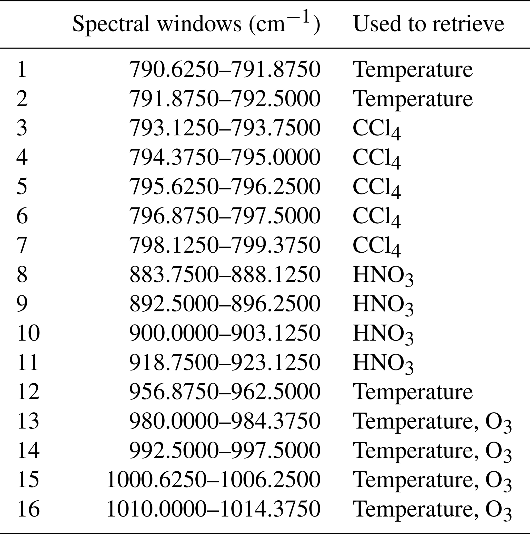
The retrieval data generated for this article were optimised to determine temperature, CCl4, HNO3, O3 and aerosols. The spectral windows used for the optimised retrieval are listed in Appendix A1. A total of 16 channels were used in the retrieval, each for a different purpose (3 for temperature, 5 for CCl4, 4 for HNO3, and 4 for temperature and O3 combined). The retrieval was conducted using Laplacian regularisation implemented using a Delaunay triangulation-based irregular grid-capable discretisation (Krasauskas et al., 2019). The Laplacian (second-order derivative) regularisation replaced the traditional first spatial derivative regularisation approach. The Delaunay technique reduces the computational cost of the tomographic retrieval. This flight was the first GLORIA limited-angle tomography retrieval with this method.
To examine the robustness of our results, we tested different retrieval configurations. We found the derived temperature product to be robust within the region of high tangent-point4 density, whereas other parts of the volume were subject to large differences depending on the chosen a priori or regularisation. The a priori used in the retrieval is a smoothed ECMWF analysis and WACCM (Whole Atmosphere Community Climate Model) reanalysis field.
2.2 GROGRAT – Gravity-wave Regional Or Global Ray Tracer
GROGRAT is a ray-tracing tool that traces the propagation path of a GW and can be used for both forward and backward tracing (Marks and Eckermann, 1995; Eckermann and Marks, 1997). GROGRAT is based on the GW dispersion relation:
where ω is intrinsic frequency, N is Brunt–Väisälä frequency, f is Coriolis frequency, H is scale height, and k, l and m are wavenumber in the x, y and z direction. A GW packet is fully characterised by its position in space and time as well as its 3D wave vector. The ray tracer projects this state vector forward or backward according to the ray-tracing equations (Lighthill, 1978):
where i denotes the spatial direction (x,y or z), and is differentiation in time.
In this study, the 4D version of GROGRAT is used. This means that the background (see the next section to see how the background state was determined) temperature, wind and pressure (from ERA5 reanalysis) change with time. For each time step of the ray integration the group velocity and state vector (x, y, z, t, ωgb, k, l, where gb indicates ground-based) change. Along the ray path, wave action density5 is conserved, but GW saturation and GW dissipation by radiative damping and turbulence are taken into account (based on the scheme developed by Zhu, 1993). Gravity wave amplitudes are converted from wave action.
For back tracing, it is important to keep in mind that the GW can be emitted at any point along the ray and is not necessarily emitted at the lowest point of the ray (see Preusse et al., 2014). One indication of a GW source along the ray is a violation of the Wentzel–Kramers–Brillouin (WKB) approximation (Hertzog et al., 2001). In GROGRAT this is tested via the parameter (see Eq. 5 of Marks and Eckermann, 1995)
This implementation of the WKB approximation requires that the scale of change of the wavenumber is large compared to the wavelength of the GW.
2.3 Reanalysis data and model integrations
Throughout this study (except Sect. 4) we use the ERA5 (European Centre for Medium-Range Weather Forecasts Reanalysis 5th Generation Description; Hersbach et al., 2020) reanalysis. The ERA5 data are interpolated to a 0.3∘ × 0.3∘ × 200 m grid. All data used in this article are on a geopotential height grid (with the exception of Fig. 1 and the calculation of the cross-stream ageostrophic wind in Sect. 4, which is calculated on a pressure grid).
To investigate the influence of orography, in Sect. 4 two global model forecasts with the ECMWF Integrated Forecast System (IFS) are discussed: (i) CTL-run and (ii) T21-run. The forecasts are performed at TCo1279 horizontal resolution (corresponding to 9 km grid spacing on a cubic octahedral grid) with 137 vertical levels and use the operational ECMWF IFS configuration of cycle 45r1 (https://www.ecmwf.int/en/forecasts/documentation-and-support/evolution-ifs/cycles/summary-cycle-45r1, last access: 29 April 2021). The only difference in the two runs is the resolved orography field, which in CTL-run is at TCo1279 resolution and in T21-run at T21 resolution. This means that the orography in T21-run is much smoother and does not resolve, for instance, Fjords at the Greenland coast, and it is only 60 % of the TCo1279 orography field elevation. The two forecasts were initialised on 9 March 2016 at 12:00 UTC and run freely for 72 h (the GW observation takes place 30 h after initialisation).
The model output and reanalysis data were separated into GWs and the large-scale background state. Zonally the data were separated with a fast Fourier transform, assuming that zonal wavenumbers up to 12 can be attributed to the large-scale background and that higher zonal wavenumbers are attributed to GWs (Strube et al., 2020). In the two remaining directions, a Savitzky–Golay (Savitzky and Golay, 1964) filter was applied. A third-order polynomial was applied in the y (across-latitude) direction with a 50-point smoothing – 15∘ of latitude. A fourth-order polynomial was applied in the z (vertical) direction with a 15-point smoothing – 3 km. The GW field (called the residual) remains after subtracting the large-scale background from the original model field. A comparison of different background removal methods can be found in the Appendix of Krisch et al. (2020).
2.4 Jet geostrophic balance calculation
A jet can generate GWs if an imbalance exists between the Coriolis and the pressure gradient forces in the momentum equation (Zülicke and Peters, 2006). The area of imbalance normally occurs in the jet exit region and can radiate GWs spontaneously in an attempt to balance the Coriolis and pressure gradient forces. The cross-stream ageostrophic wind speed or the cross-stream Lagrangian Rossby number can be used to diagnose an out-of-balance jet (Zülicke and Peters, 2006; Mirzaei et al., 2014; Plougonven and Zhang, 2014, e.g.). Similar to Mirzaei et al. (2014), it was found that similar results are obtained for both, with less noise when using the cross-stream ageostrophic wind speed.
In this article, the cross-stream ageostrophic wind is used to diagnose unbalanced flow within the jet as suggested by Mirzaei et al. (2014). Firstly, horizontal wind (u and v components) and geopotential height fields were smoothed to remove GW signatures with a boxcar6 over 500 km in the x and y direction (similar to Mirzaei et al., 2014). Secondly, ageostrophic winds (ua and va) were calculated from pressure-level data using MetPy (May et al., 2008–2020). Thirdly, the cross-stream ageostrophic wind was calculated using the approach of Zülicke and Peters (2006).
In a final step it was tested whether this quantity exceeds the threshold of 7.5 m s−1, which corresponds to a critical Rossby number of 0.15 and a length scale of 500 km. In this case we consider this unbalanced region for GW emission.
3.1 Synoptic situation
The synoptic situation for our case study is shown in Fig. 1. The meandering 300 hPa geopotential height and horizontal wind field show a cyclonically breaking Rossby wave. At flight time (10 March 18:00 UTC, panel b), the potential vorticity lines steepen and turn back at the point of inflection, signalling Rossby wave breaking. An associated mid-tropospheric low-pressure system drifts from west to east (not shown). Accordingly, the sub-tropical jet drifts with time. However, the divergence of the winds within the jet remains above or in close vicinity of Greenland throughout the 30 h before observation. The above-mentioned synoptic conditions are favourable for the formation of jet-generated GWs (e.g. Uccellini and Koch, 1987; Plougonven and Zhang, 2014).
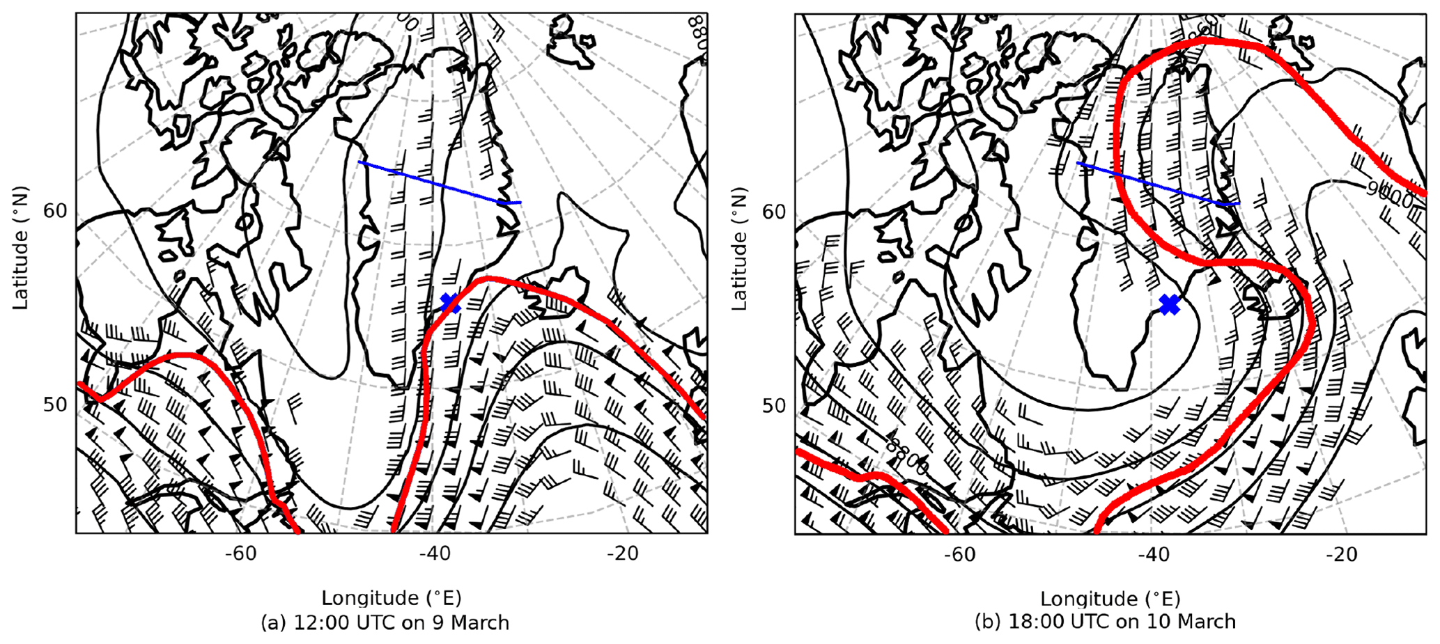
Figure 1ERA5 geopotential heights and winds at 300 hPa valid for 9 March at 12:00 UTC (a) and 10 March at 18:00 UTC (b). Only wind speeds greater than 20 m s−1 are plotted. One full barb represents 10 m s−1 and half a barb 5 m s−1. The red line represents the approximate (excluding eddies and local fluctuations) 4 potential vorticity units ( m2 K s−1 kg−1) line. The blue cross will be referred to in Sect. 3.3. The blue solid line represents the flight section used for GLORIA retrieval.
A trapping layer inhibits GW propagation beyond the respective layer. A trapping and reflection layer is formed by an increase in wind speed and stability and is identified with the help of the Scorer parameter (e.g. Durran, 2003; Geldenhuys et al., 2019). Knowing potential GW reflection layers can therefore be important to find the sources of GWs. The Scorer parameter over the southern mainland of Greenland (not shown) indicates multiple reflection layers between 7.5 and 13 km. However, further investigation reveals that up to 30 h before observation all horizontal wavelengths > 4 km will propagate through these reflecting layers. With no reflecting layers present for the wavelengths considered in this study, it is clear the GW source can be located at the surface or in the free troposphere. Furthermore, this justifies the use of ray-tracing tools for freely propagating GWs (Sect. 3.3).
A jet is known to release upward-propagating (above the jet) and downward-propagating (below the jet) GWs (Thomas et al., 1999; Guest et al., 2000). Hodographs can be used to distinguish between upward- and downward-propagating GWs. In the Northern Hemisphere clockwise (anticlockwise) rotating hodographs indicate upward-propagating (downward-propagating) GWs (Andrews et al., 1987; Hertzog et al., 2001). Multiple hodographs from the ERA5 reanalysis were drawn within the 500 and 300 hPa jet region. The hodographs (e.g. Fig. 2) depicted no rotation to weak clockwise rotation with altitude below 7 km, with strong clockwise rotation above 10 km. The rotation above 10 km is nearly circular, which implies that . This points to an upward-propagating inertia–gravity wave with a low intrinsic frequency close to the Coriolis parameter (Hertzog et al., 2001; Fritts and Alexander, 2003). A nearly full anticlockwise rotation is less pronounced between 7 and 10 km, even though this altitude range should be treated with care as the jet region (7.5 to 10 km at flight time) can present artificial results.
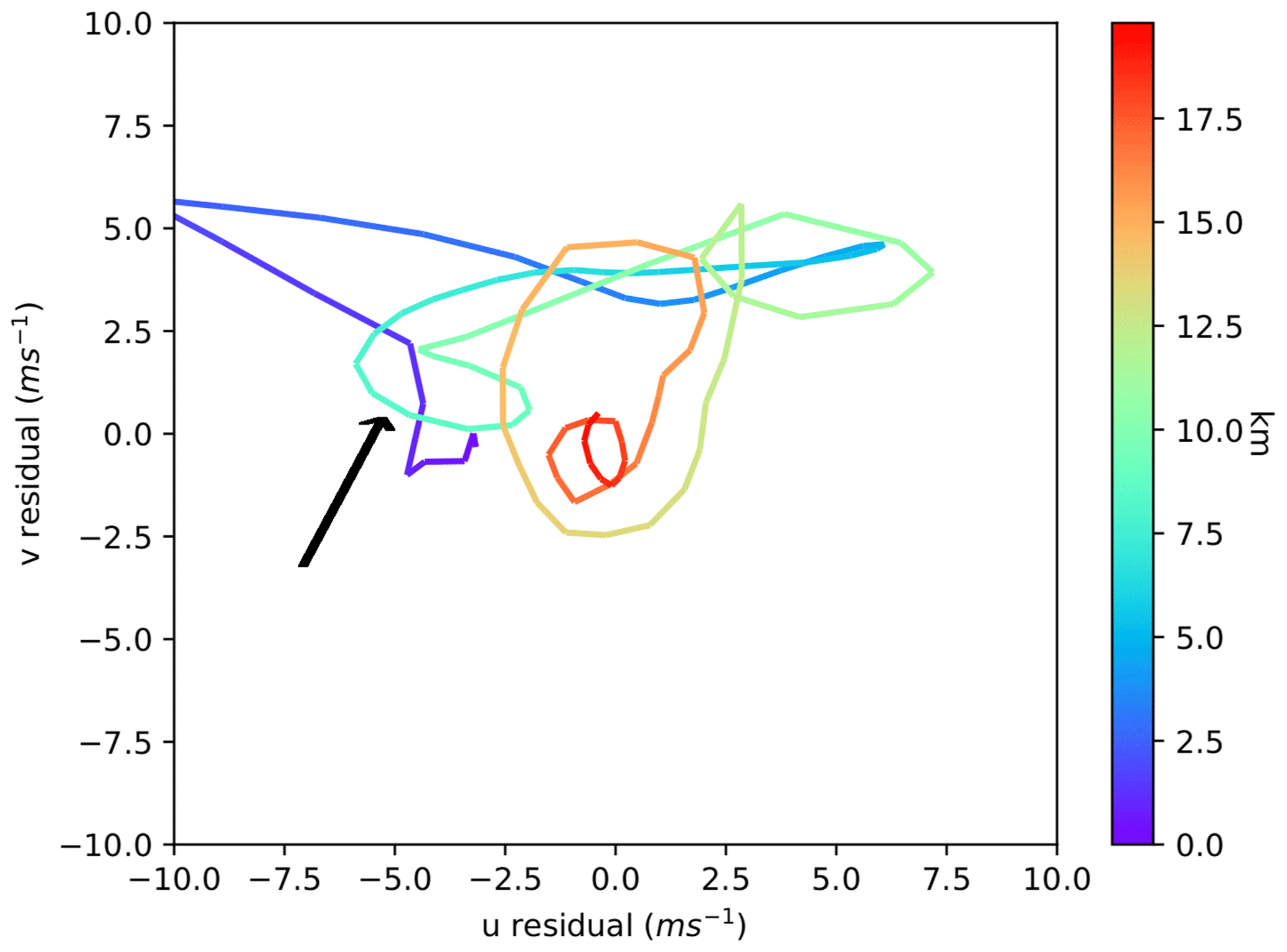
Figure 2Hodograph in the centre of the jet upwind of Greenland at 60∘ N and −30∘ E. The arrow points to the anticlockwise rotation between 7 and 10 km, with the rest being clockwise or no rotation. The hodograph is valid for 9 March at 07:00 UTC, calculated from ERA5, and is a good representative for all hodographs upwind, within the jet and through time.
High-resolution ECMWF medium-range weather forecasts predicted a large-scale GW event covering most of Greenland 2 d before the flight was performed. Accordingly, a PGGS research flight was planned to measure these GWs, presumably generated by the breaking Rossby wave. HALO flew from Kiruna (Sweden) to Greenland where it crossed the mainland from south-east to north-west at 10.5 km and, on the way back, at 13.5 km. The temperature field presented in this article is retrieved from this higher leg (black line crossing Greenland in Fig. 3) from 19:00 UTC (Universal Time Coordinated) to 21:00 UTC. Throughout this article, the closest synoptic time (18:00 UTC) is referred to as flight time.
3.2 GLORIA observations
Gravity waves are seen within the tangent-point area in Fig. 3. Outside this area the retrieval does not have measurement information and falls back to the a priori. The GWs within the tangent-point area compare well to ERA5 data (more on this in Sect. 3.3). In the horizontal (panel a), the GW phase fronts are oriented at about a 90∘ angle to the flight path. With height (panel b), the phase fronts slant eastwards. Slanting GW phase fronts are an indication of vertically propagating, internal GWs. The observed slant together with the hodograph analysis indicate upward propagation, with intrinsic propagation to the east.
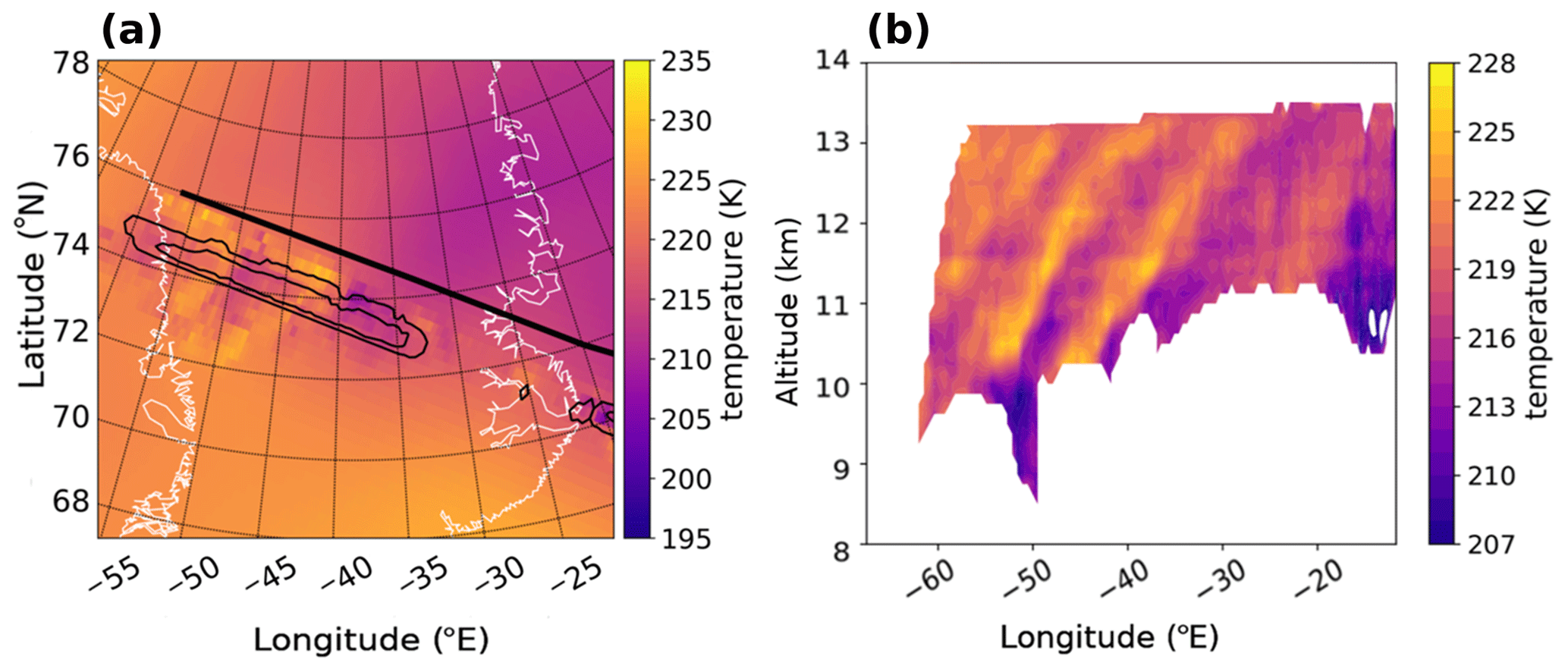
Figure 3Horizontal (a) and vertical (b) cross section of the GLORIA temperature retrieval, showing the retrieved GW packet. The horizontal cross section is shown for 11 km. The white line represents the Greenland coastline. The thick black line represents the section of the flight path that was used for the retrieval, and the thin black contours represent the tangent-point area. The vertical cross section is averaged at 90∘ to the flight path using only data within the tangent-point area. Note the decrease in vertical wavelength and amplitude above 12 km.
The GW characteristics are determined within the tangent-point area indicated in Fig. 3 and similar retrieved images. The characteristics of these GWs are listed in Table 1 and were used as input into GROGRAT (see next section). A horizontal wavelength between 320 and 390 km is observed in different parts of the GW packet. The vertical wavelength is between 1.6 and 2.1 km, and the GW orientation is between 130 and 140∘ from the north. The amplitude and vertical wavelength decrease with altitude (as can be seen in Fig. 3b). This is indicative that a change in propagation conditions is taking place and can point to GW dissipation (more on this in Sect. 3.3).
Table 1GW characteristics determined by eye from the retrieval (Fig. 3). The wavelengths are represented by λh and λz for the horizontal and vertical direction, respectively. Ray nos. 0 to 3 were used as input for the GROGRAT ray tracer.

3.3 GROGRAT ray tracing
Tracing the backward trajectory of a GW is an established method to find its source (e.g. Marks and Eckermann, 1995; Krisch et al., 2017, 2020). According to Hertzog et al. (2001), the excitation of GWs by geostrophic adjustment from the jet is usually associated with enhanced values of the WKB parameter (δ) near the height of the wind maximum. This is attributed to the sharp upper and lower edges of the jet. Sharp changes in the jet wind speed will induce sharp changes in the vertical wavenumber. If the scales of change in the wavenumber become large compared to the wavelength, the WKB parameter is violated (see Eq. 4 and corresponding Sect. 2.2).
Four main rays were back-traced, starting between 11 and 12.3 km based on the GW parameters given in Table 1. The GW ground-based frequency or input to GROGRAT was calculated via the dispersion relation (Eq. 1) using the horizontal and vertical wavelength in Table 1 as well as ERA5 reanalysis data.
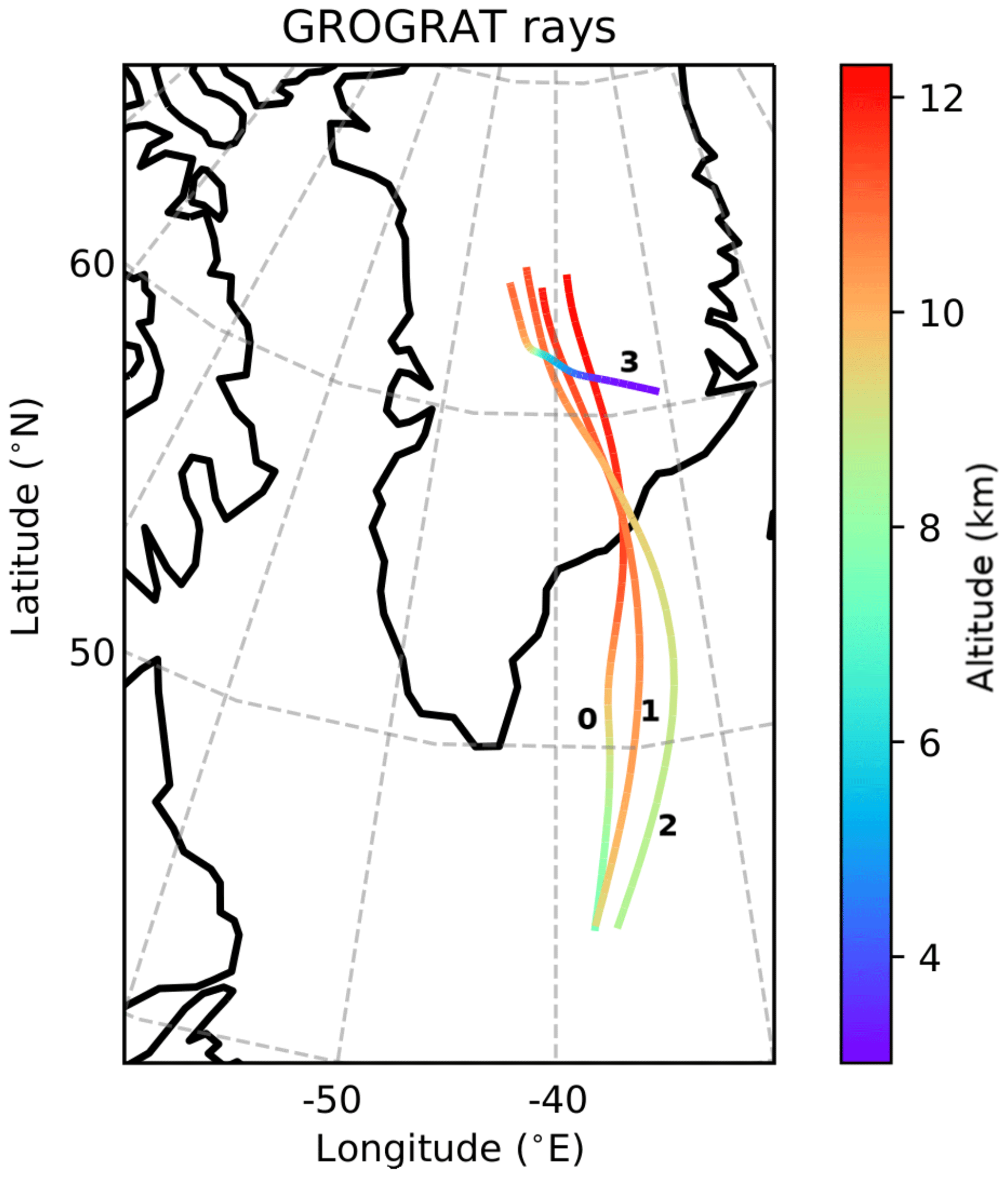
Figure 4GROGRAT back-tracing rays using a 4D setup. The rays have a starting time of 10 March 2016 at 18:00 UTC. The initial conditions for the rays are listed in Table 1. The back tracing starts between 11 and 12.3 km and is depicted with respect to altitude, latitude and longitude.
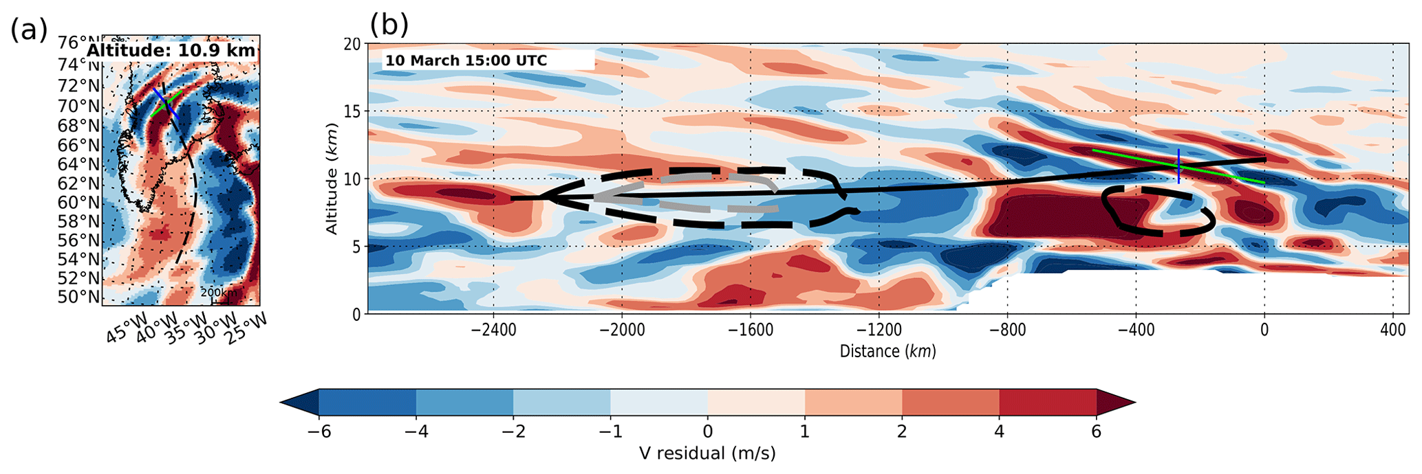
Figure 5GROGRAT back tracing of ray no. 2 and meridional wind (v) residuals from ERA5. The back tracing starts at 11.4 km (on 10 March at 18:00 UTC) and ends at 8.5 km (on 9 March at 18:00 UTC). (a) The horizontal cross section of the ray path (dashed black line) and the corresponding v-residual wind speeds at 10.9 km. (b) The vertical cross section of v-residual wind speeds along the ray path (solid black line). Ray tracing started at ray reference time 42 h (flight time), and both (a) and (b) are valid for 13:00 UTC (5 h prior to ray initialisation). The cross of the blue and green line represents the position of the GW at the respective time; the blue line indicates one horizontal (vertical) wavelength in the horizontal (vertical) cross section, and the green line indicates the orientation of the phase fronts, all calculated in GROGRAT. The thick dashed black line indicates cross-stream ageostrophic wind values in excess of 7.5 m s−1. The encircled dashed area at −1500 km occurred between 24–19 h before ray initialisation (the back trace passed through this area at the same time). The encircled dashed area at −400 km represents an out-of-balance jet at 2–7 h before ray initialisation.
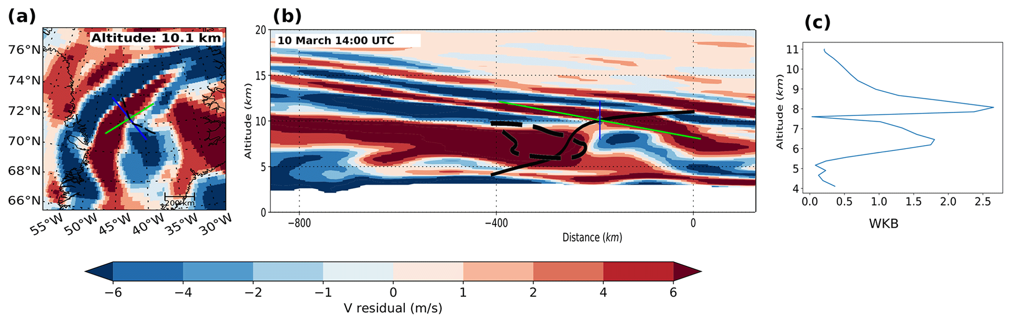
Figure 6Similar (a and b) to Fig. 5, but valid for ray no. 3 on 10 March at 14:00 UTC (4 h prior to ray initialisation). The horizontal cross section (a) is valid for 10.1 km. Panel (b) shows that the ray tracing starts at 11 km and ends above the Greenland plateau. The thick dashed black line indicates cross-stream ageostrophic wind values in excess of 7.5 m s−1. (c) The WKB parameter with height. The WKB parameter can be related to the jet in Fig. 8.
All rays trace backward into the jet and end over the ocean, with the exception of ray no. 3 (Fig. 4; rays named as in Table 1), as the vertical cross section of the GLORIA observation indicates the GW is propagating intrinsically opposite to the wind. The horizontal group velocity, however, is slower than the wind velocity, which leads to a downstream drift of the GW packet. To provide further confidence in the ray-tracing study, sensitivity tests were performed. An ensemble ray trace (20 members) was conducted by perturbing the initial conditions (listed in Table 1) by ≈ 10 %: ±0.2 km for the vertical wavelength and ±30 km for the horizontal wavelength. This is the approximate error associated with the wavelength determination from Fig. 3. All ensemble members behaved similarly to the main rays (Fig. 4). The ray paths proved to be more sensitive to the launch orientation. A 10∘ change in orientation frequently ended with the back-traced GW being evanescent or vertically stalling. In another experiment, the four main rays were back-traced, whereby the ray orientation at the end of the ray was perturbed (again by 10∘) and forward-traced. In the forward tracing, a change in orientation was much less sensitive.
Ray nos. 0 to 2 (named as in Table 1) all experienced large horizontal propagation and very little vertical propagation. This is normally characteristic of trapped GWs; however, the slanted phase fronts in Fig. 3 indicate that the GWs were not trapped. Only ray no. 2 is discussed here in detail (Fig. 5). The wavelengths and phase orientation predicted by GROGRAT correlate well with the ERA5 reanalysis and produce further trust in the experiment (same as for ray no. 3 – Fig. 6). The GROGRAT-calculated vertical group velocity peaks at 10 km with 0.2 m s−1 and has a minimum of 0.05 m s−1 at 9 and 11 km (Fig. 7). This translates to a vertical propagation speed of 180 to 720 m h−1. Intrinsic horizontal group velocity peaks at 72 m s−1 and has a minimum of 25 m s−1. This translates to a ground-based group velocity ranging from 6 to 17 m s−1.
The cross-stream ageostrophic wind (calculated as described in Sect. 2.3) indicates out-of-geostrophic-balance flow within the jet exit region at multiple locations along the ray path (Fig. 5). In this study, we use a safe value of 7.5 m s−1 to indicate that the jet exit region is out of balance and can spontaneously emit GWs. Mirzaei et al. (2014) used 1 m s−1 to indicate out-of-balance areas in the jet and argued theoretically that 4 m s−1 is a good value. In Fig. 5 at km the ray passes through a 10 m s−1 cross-stream ageostrophic wind region 22 h before observation. Multiple other out-of-balance regions exist within the jet throughout the ray lifetime. From this, it is concluded that the jet is constantly emitting GWs. It is noted that ray nos. 0 to 2 did not have major WKB violations. Although WKB values reached a maximum within the out-of-geostrophic-balance jet regions, the peak values reached merely 0.5.
Ray no. 3 is the only GW which traces to the orography (Fig. 6) and was hence investigated for a possible mountain wave. The ray traces to the plateau of Greenland and not the precipitous coastline orography. In addition, the ray passes through a cross-stream ageostrophic wind region at the steepest part of the ray. Clear violations are observed in the WKB values at 6.5 and 8 km (consistent with the findings of Hertzog et al., 2001), supporting the idea that the GW is released by the jet. It should be noted that cross sections through ERA5 reanalysis residual data did indicate mountain wave activity localised in time and space along the coast. However, as far as the GROGRAT experiment is concerned, these mountain waves were not observed by GLORIA. Ray no. 3 was emitted by the jet initially with a longer vertical wavelength (hence the steep propagation path at km), which was immediately reduced as it propagated out of the strong wind regime. The vertical group velocity peaked around 8 m s−1 (Fig. 7), receding rapidly to 0.04 m s−1 at 11 km.
The vertical wavelength of ray nos. 0 to 2 similarly decreased as the GW passed above the jet region (Fig. 7 left). The effect of the changing vertical wavelength is also observed in the vertical group velocity (Fig. 7 right). Similarly, the observed GW amplitude and the observed vertical wavelength decrease with height (Fig. 3 and Table 1); this can imply that the GWs are approaching dissipation. A large drop in background wind speeds (17 m s−1 for ray no. 3 and 40 m s−1 for ray nos. 0 to 2) occurs from 8 to 9 km to the ray starting altitude (Fig. 8). Within the same region the stability of the atmosphere changes dramatically within the jet exit region (location indicated by the blue cross in Fig. 1). Stability changes from 0.00025 K per 100 m between 8 and 12 km to 0.2 K per 100 m between 12.5 and 15 km are observed. Although this greatly resembles a wave duct, the GWs in this study are not reflected (see the previous discussion in Sect. 3.1).
The strong decrease in wind speed is responsible for the decrease in the vertical wavelength and hence responsible for the GW dissipation. As the wind speed approaches the horizontal phase velocity (Fig. 8), the intrinsic frequency decreases to zero, which means the vertical wavenumber will approach infinity, representing a critical layer for the GW.
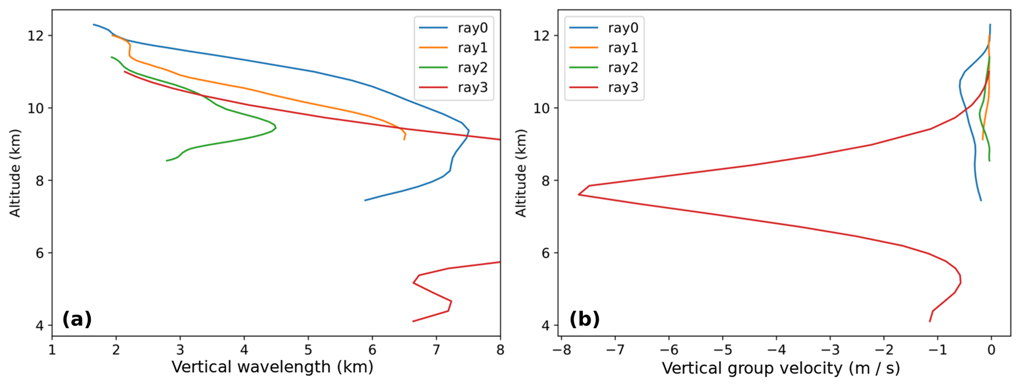
Figure 7Vertical wavelength (a) and vertical group velocity (b) along the back trace for ray nos. 0 to 3 as calculated by GROGRAT. The leftmost plot is cut at 8 km in order to achieve readability for ray nos. 0 to 2.
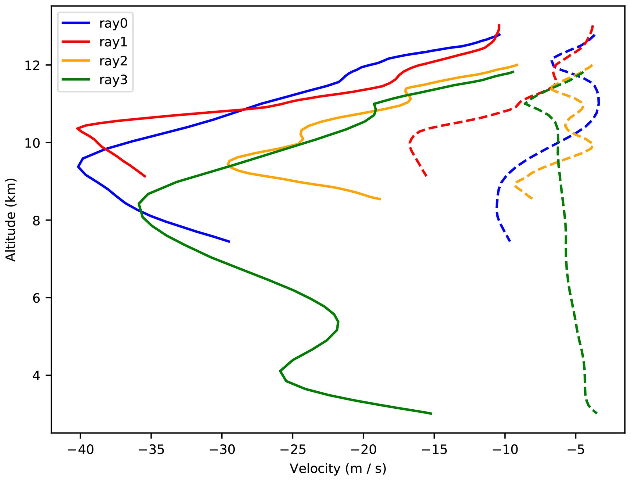
Figure 8The horizontal phase velocity (dashed) and the background wind (solid) along ray nos. 0 to 3. Where the phase velocity and the wind speed approach one another a critical layer exists. Altitudes above the ray starting point (Table 1) represent the same starting conditions ray-traced forward.
Originally designed as an attempt to entirely rule out topography as a source, a numerical experiment with strongly reduced topography was designed. This yielded unexpected results implicating topography as a major contributor.
4.1 Numerical experiment overview and results
The unmodified ECMWF operational model was used as the control (CTL-run, Sect. 2.3) (Fig. 9a–h). CTL-run produced GWs (Fig. 9e) similar to observations (Fig. 3) and ERA5 data (Figs. 5 and 6).
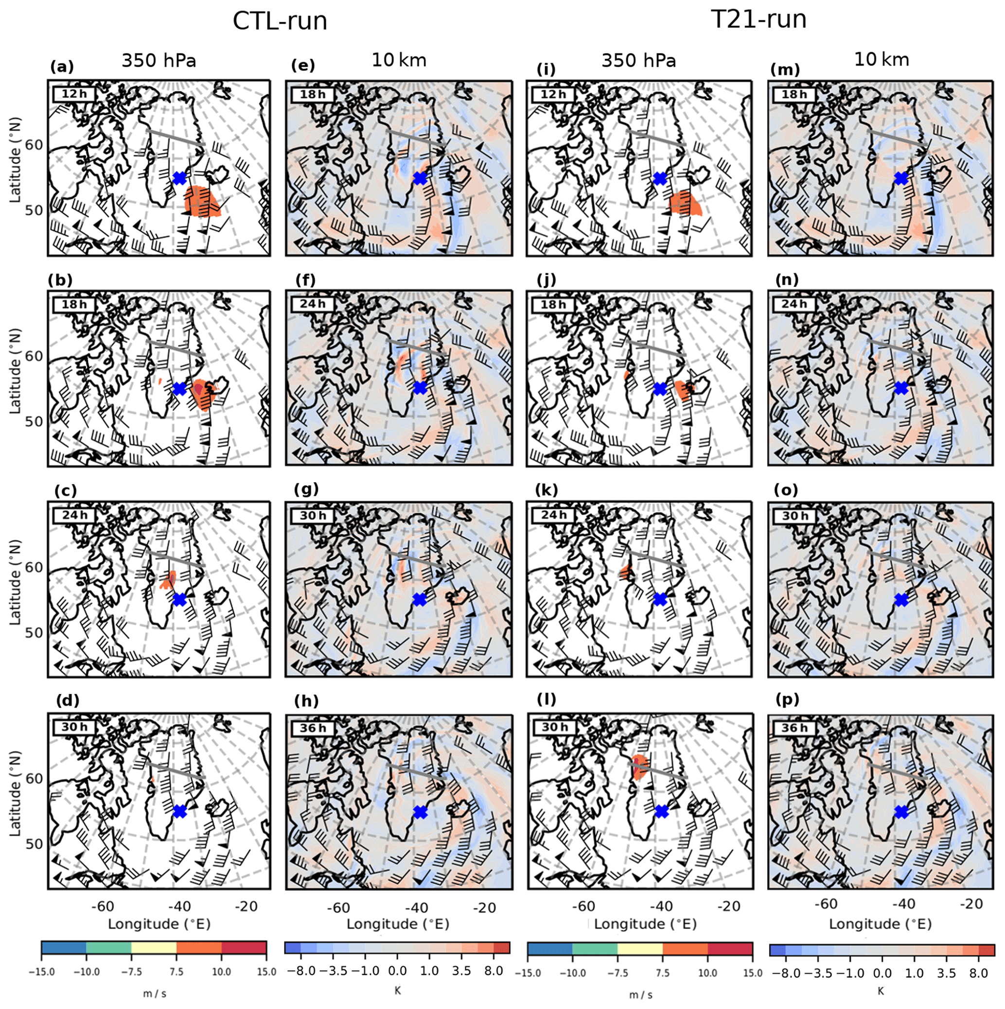
Figure 9CTL-run (a–h) and T21-run (i–p) cross-stream ageostrophic wind and temperature residuals at different times. The cross-stream ageostrophic wind (a–d and i–l) was calculated from pressure levels; hence, here it is depicted at 350 hPa (≈ 8.1 km). The temperature residuals (e–h and m–p) were determined based on geopotential heights; hence, this is valid for 10 km. The temperature residuals are depicted ≈ 2 km higher than the cross-stream ageostrophic wind, as the GW structure forms a complex interference pattern with upward- and downward-propagating GWs within the jet. The temperature residual plots are offset by 6 h from the cross-stream ageostrophic wind to allow time for the GWs to propagate to 10 km (a vertical group velocity of 200–700 m h−1 indicates vertical propagation of 2 km between 3 and 10 h). The overlaid wind barbs are as in Fig. 1. The flight path is indicated in grey, and thick black lines represent the coastline. The blue cross indicates the location of the stability discussion in Sect. 3.3. Times (in h) are since model initialisation (on 9 March at 12:00 UTC) + xx h (“xx” as specified in the top left corner of each panel).
The second experiment (T21-run) uses a T21 topographic field (the lowest-resolution topographical field available) to achieve a smoothed orography. Comparing CTL-run with T21-run on 10 March at 18:00 UTC (Fig. 9e and m), in the area of interest GWs are observed in CTL-run, but hardly any are seen in T21-run (also seen in the following time steps). The very weak GWs observed in T21-run exist from the very first model time step, and no new GWs are forced in the following time steps. Clearly, the topography plays a significant role in GW generation. Are the two experiments hence an indication of direct orographic GW generation? Keeping in mind that Sect. 3.3 implicated the jet as the likely source, this hint to orography is a puzzling result. We therefore investigate the hypothesis that the orography is responsible for the GW excitation in an indirect way.
4.2 CTL-run vs. T21-run: what is the difference?
Which synoptic-scale differences then arise from the reduced orography that could induce GW excitation? As argued in Sect. 3.3 the GWs are likely excited by out-of-geostrophic-balance flow. Therefore, we compare the cross-stream ageostrophic wind (calculated as in Sect. 2.3) for the two model runs. In Fig. 9, the cross-stream ageostrophic wind is shown when all three following conditions are met: the values of the cross-stream wind are greater than 7.5 m s−1, the total wind speed is greater than 20 m s−1 and latitudes are lower than 80∘ N. As mentioned in Sect. 3.3, a critical value of 7.5 m s−1 is used to indicate when the jet can spontaneously radiate GWs.
CTL-run, in Fig. 9, has large cross-stream ageostrophic wind regions. These cross-stream ageostrophic wind regions are an indication of an imbalance between the Coriolis and the pressure gradient force in the jet. Early after model initialisation (12 and 18 h – Fig. 9a and b), CTL-run indicates large out-of-balance jet regions over the ocean. Figure 9b depicts the CTL-run jet reaching cross-stream ageostrophic winds of 10 m s−1, and 6 h later the CTL-run jet is unbalanced over the Greenland mainland (Fig. 9c). The greater the cross-stream ageostrophic wind is, the more unbalanced the jet is, and the more likely it is to spontaneously emit GWs (Zülicke and Peters, 2006; Mirzaei et al., 2014).
After each imbalance in the jet a GW response is seen 6 h later 2 km higher and downwind of the imbalance region (comparing Fig. 9a–c with e–g). This height and area offset is understandable as the GWs take time to propagate from 8 to 10 km while drifting horizontally. Taking the mid-range vertical group velocity of ray no. 0 (Sect. 3.3), the GW packet will propagate 2.7 km vertically in 6 h. Throughout all shown time steps the unbalanced region is associated with a GW field downwind.
T21-run (Fig. 9i–p) shows a totally different picture. Firstly, the cross-stream ageostrophic wind indicates a smaller region and a more balanced jet. Small regions of 7.5 m s−1 (no 10 m s−1 region) are seen over the ocean in Fig. 9i and j. No cross-stream ageostrophic wind is observed upstream or over the Greenland mainland at 24 h after model initialisation (Fig. 9k). Matching the more balanced jet, GWs are almost nonexistent in T21-run.
Only during one time step was the T21-run jet more unbalanced than CTL-run (Fig. 9d and l). At forecast hour 30 (at flight time) a large area of imbalance occurs below the north-westernmost part of the flight track (Fig. 9l). This imbalance area (at 350 hPa) is larger in T21-run and indicated cross-stream ageostrophic wind values exceeding 10 m s−1. A total of 6 h later, T21-run indicated more GWs than the previous time step (north of the flight track – Fig. 9p), and for the first time, a GW field comparable to (if not a greater than) CTL-run (Fig. 9h) was observed.
CTL-run, in Fig. 9, has larger and more intense cross-stream ageostrophic wind regions when compared to T21-run. Throughout all shown time steps the greater unbalanced region has a greater GW field. Therefore, we assert that the GWs are directly caused by the increased lack of balance within the jet.
In order to find direct evidence for the presence of GWs upstream of Greenland, divergence is considered. Divergence fields are frequently used to differentiate between GWs and balanced motions (Zülicke and Peters, 2006). Besides the emphasis on shorter scales by differentiation, this method removes the geostrophic modes and leaves the ageostrophic flow including GWs. We have applied this to the potential source region of the GWs upstream of Greenland for Fig. 10. At 6 h after model initialisation (left) we see a superposition of wave phase fronts parallel to the isobars and perpendicular to the flow between the blue cross and Iceland. The latter is likely to become the waves we observe later with GLORIA. At 18 h (right) the two directions of phase fronts have separated, forming long streaks parallel to 30∘ W south-west of Iceland and an arc of phase fronts perpendicular to the flow between Iceland and Greenland. These GWs upstream of the Greenland coast are consistent with our hypothesis that flow instability upstream of the terrain is the source of the GW patterns. Furthermore, the source moves with the jet and drifts over Greenland in later time steps.

Figure 10Divergence for CTL-run at 6 and 18 h after model initialisation. The divergence is indicated at 8.2 km to correspond to the cross-stream ageostrophic wind at 350 hPa in Fig. 9. The overlaid pressure isolines (thin black lines) give an indication of the geostrophic wind direction. The thick black lines, blue cross and times in the top left corner are as in Fig. 9.
4.3 CTL-run vs. T21-run: what causes the difference?
If CTL-run has GWs and T21-run does not, then the difference between the two model runs must be the source of the GWs. By now we have established that the jet and its related imbalance are the cause of the GWs. We know that the orography played a role in the balance of the jet, but we are missing a puzzle piece connecting these two.
Comparing the two model runs, the jet location and shape remained similar. The centre of the low pressure (being stronger in T21-run) was displaced ≈ 5∘ westwards (Fig. 11). To find the missing link the difference in the model basic variables (U, V, temperature, pressure and relative vorticity) was calculated. Subtracting the wind speed and relative vorticity of T21-run from CTL-run produced an interesting dipole structure (Fig. 12). In Fig. 12e–h green (brown) demarcates an area where the CTL-run wind speed was faster (slower) than T21-run. In order to investigate the origin of this difference, it is convenient to calculate relative vorticity.
It is well known that an uplift process induces relative vorticity (Holton, 2004). It then should be remembered that relative vorticity is only a different expression for the same wind field and that any process which causes changes in vorticity alters the wind velocity field.7 Indeed, we find the same dipole structure which we observed in the wind velocity in the relative vorticity but offset by 90∘. The dipole structure in the wind speed and vorticity represents the changes that occurred in the wind speed and consequently the changes that occurred in the jet.
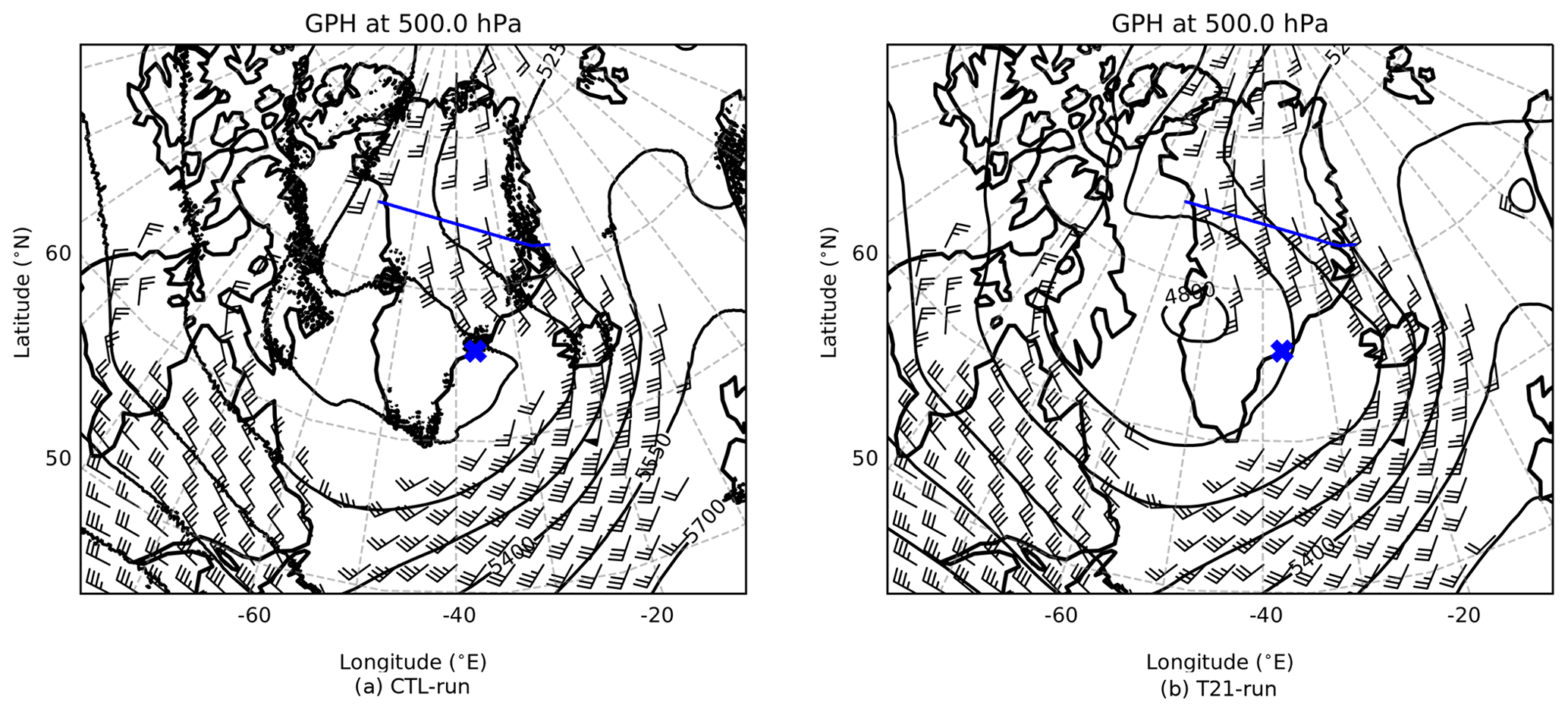
Figure 11Geopotential heights and winds at 500 hPa valid for 9 March at 18:00 UTC for CTL-run (a) and T21-run (b). Note that the spotted (especially along the coastlines) CTL-run is a result of the orographic GW drag parameterisation scheme. The rest of the display is the same as in Fig. 1, but with no potential vorticity line.
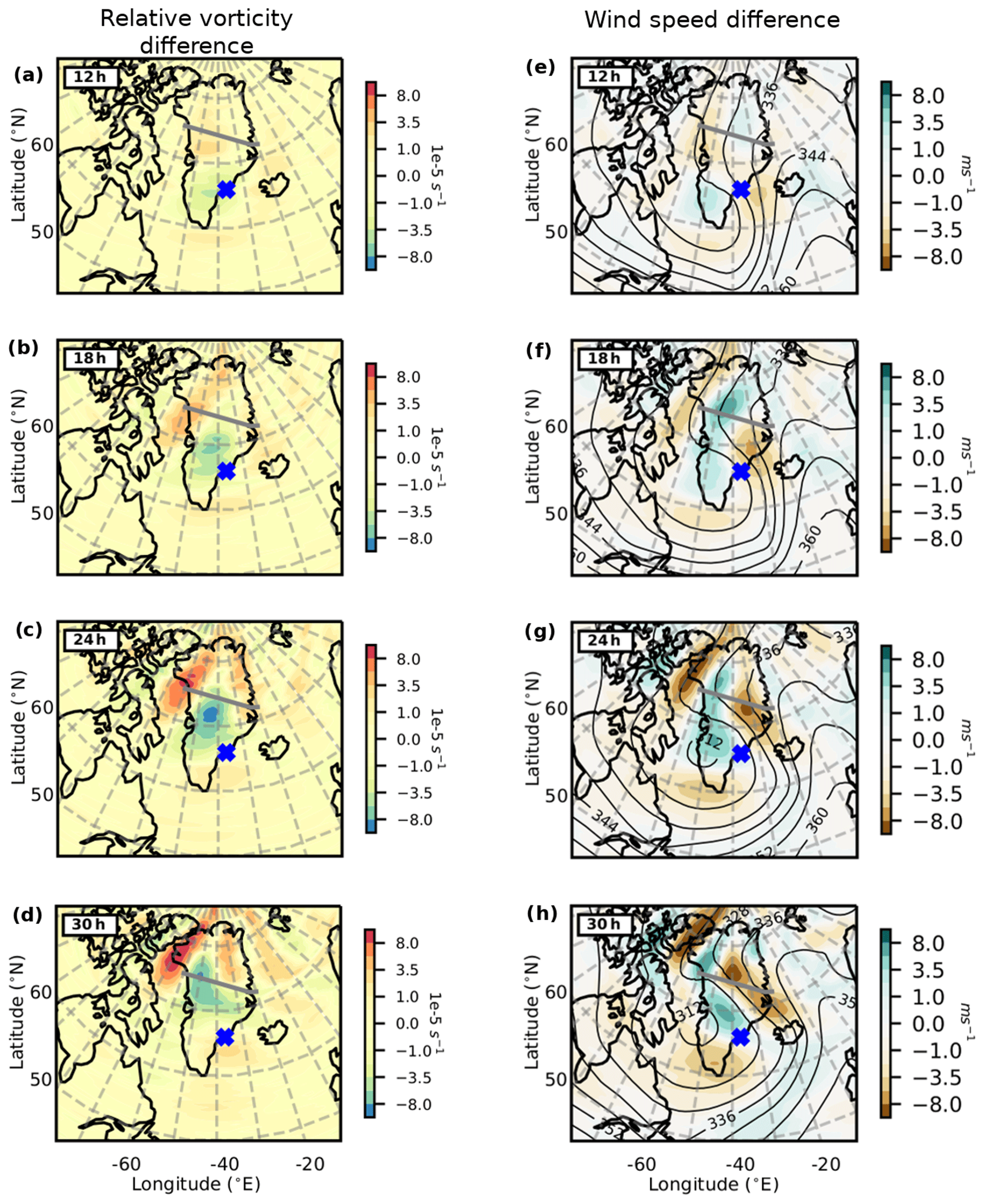
Figure 12Difference between CTL-run and T21-run for relative vorticity (a–d) and background total wind velocity (e–h) at 8 km. The revealed dipole structure is closely related to the GW excitation. The dipole structure in the wind speed difference (e–h) and the relative vorticity difference (a–d) field are offset by half a phase (90∘). Isobars (thin black line – in hPa) at the respective level are overlaid to indicate the shape of the jet. Coastline, flight path and the times indicated in the top left are similar to Fig. 9.
The role of vorticity is known from the classical formation model of a Rossby wave (Holton, 2004). The flow above the ridge is compressed by the elevated orography, changing the potential temperature gradient, which in turn changes the vorticity, deflecting the wind and the synoptic flow. For the early time steps of 12 and 18 h (Fig. 12a, b) there is a vorticity difference between T21-run and CTL-run over Greenland close to the coast. This is the same area where a change in uplift process would be expected due to the changes in the T21-run and CTL-run topography. This illustrates the effect that the uplift by orography has on the vorticity (and the jet). Later time steps (Fig. 12c–d and g–h) are more complex. We expect that the jet adjusted itself due to the lack of orography; for example, an adjustment to the orientation of the jet would additionally influence the relative vorticity field.
Vorticity can also be introduced by dissipation processes. This includes blocking (Smith, 1982), flow splitting (Siedersleben and Gohm, 2016), mountain wakes (Grubisic, 2004; Siedersleben and Gohm, 2016; Smith, 2018), breaking GWs (Siedersleben and Gohm, 2016) and wakes at the edges of mountain ranges (Grubisic, 2004). Given the location and synoptic conditions, all of the above processes most probably played a role in producing vorticity, but the dominant process (due to the altitude of the jet) is expected to be due to the compression of flow above Greenland. Equation (9) in Uccellini and Koch (1987) shows that when the vorticity (term 2 on the right-hand side) changes, divergence will also change. Uccellini and Koch (1987) and references therein found that an increase in divergence is directly linked to a more out-of-balance jet.
We note that the difference in orography from CTL-run to T21-run induced the different vorticity areas (Fig. 12). These changes in the wind field will change the components in the jet, bringing the Coriolis and pressure gradient forces out of balance. This will trigger the jet to spontaneously emit GWs in order to bring the forces back into balance. Trüb and Davies (1995) showed in an idealised model simulation that evanescent GWs form over broad terrain in flow with a Rossby number (Eq. 7) <0.25. Also, upwind and downwind of the mountain a change in the wind components was observed. For our case, using a wind of 30 m s−1, Coriolis parameter of 0.00014 s−1 and a mountain half-width measured from the blue X (Fig. 1) to the Greenland northern coast of 1650 km, a Rossby number of 0.13 is achieved from
where U is wind speed and L is mountain half-width (the width of the mountain at 0.5 × mountain height). The large evanescent GW (this should not be confused with the observations in Fig. 3, which are clearly propagating GWs), which is expected to form following Trüb and Davies (1995) over the Greenland terrain, can be one explanation for the rotation (Fig. 13) and the upstream slowdown of the wind. Wind being uplifted by orography will decrease due to kinetic energy changing into potential energy. In the geostrophic balance, the Coriolis parameter is multiplied by the wind to obtain the Coriolis force; thus, a slowdown in the wind will change the Coriolis force. The Coriolis force deflects winds to the right in the Northern Hemisphere, acting on the zonal (u) component of the wind. This explains the changes in the zonal component in Fig. 13. Figure 13 is a clear indication of the large horizontal and vertical scales over which the background wind is influenced by topography.
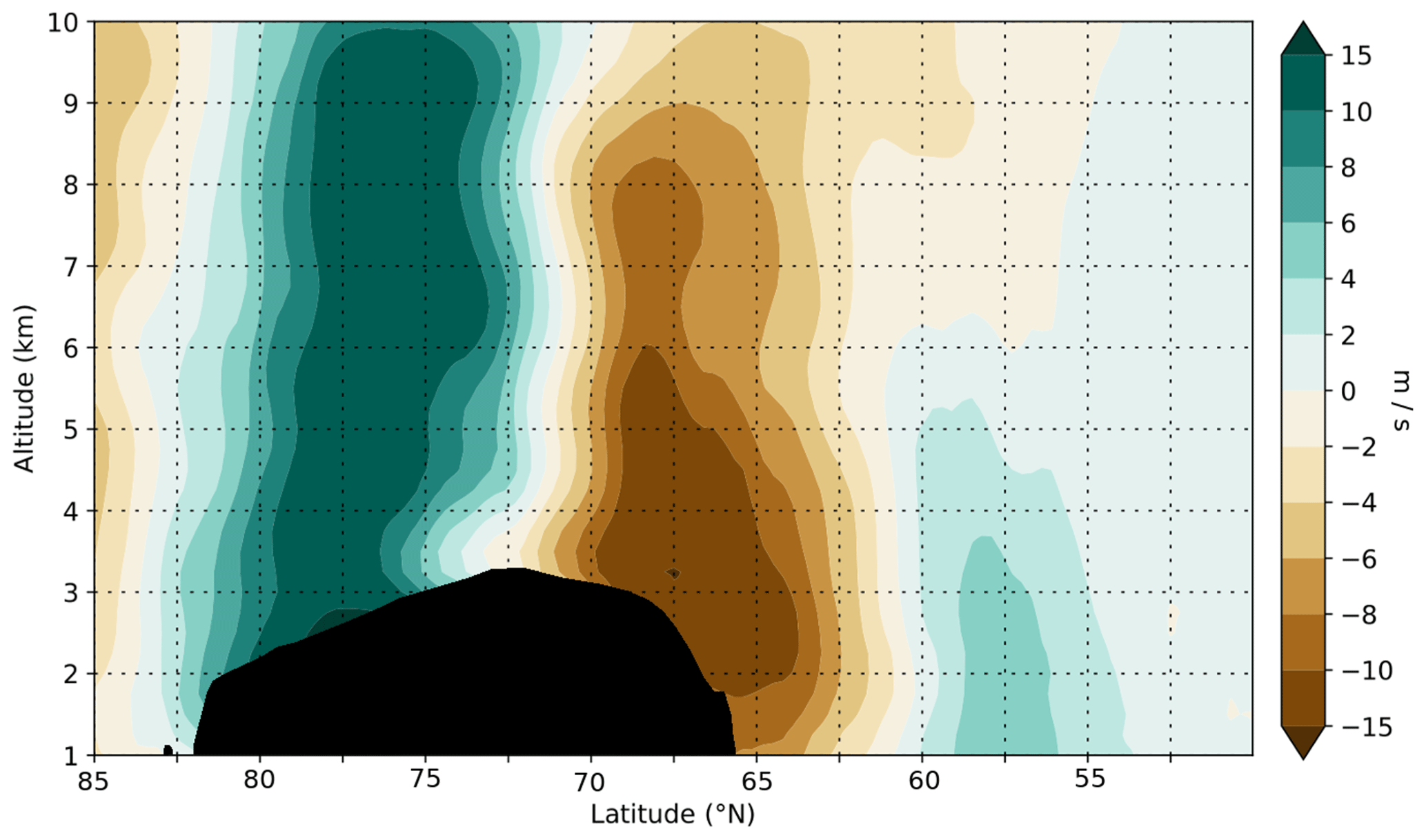
Figure 13Difference between CTL-run and T21-run zonal (u) component wind at flight time. The zonal wind component represents an along-ridge wind (similar to Fig. 11d from Trüb and Davies, 1995). The cross section with altitude is aligned roughly along the jet axis (see Fig. 1 for the jet) at 40∘ W longitude from 85∘ N to 50∘ N. Black indicates the Greenland topography.
This has been the first GLORIA limited-angle tomography retrieval using Delaunay methods and the Laplacian regularisation discussed in Krasauskas et al. (2019). Using GLORIA (Gimballed Limb Observer for Radiance Imaging of the Atmosphere), on 10 March 2016 we observed GWs over Greenland in an area where multiple possible GW sources exist. Possible GW sources include the jet or wind shear embedded in a breaking Rossby wave or orography. Observations show the GWs to have a long horizontal wavelength (≈ 330 km) and short vertical wavelength (≈ 2 km). The temperature amplitude is 4.5 K. The eastwards (upwind) tilt of the observed GW phase fronts (Fig. 3) indicates a vertically propagating GW. Using ERA5 reanalysis winds it is determined that this GW is upward-propagating. Intrinsically the GW packet propagates horizontally against the wind. Along the back trace, between 12.3 and 7.5 km, the intrinsic phase velocity varies between 25 and 72 m s−1 (ground-based velocity of 6–17 m s−1). This is very fast compared to its vertical group velocity, which is 0.05–0.2 m s−1, creating very oblique propagating GWs.
The GLORIA-observed horizontal and vertical wavelengths as well as the calculated frequency were used as input into GROGRAT (Gravity-wave Regional Or Global Ray Tracer). Back-tracing rays trace into the jet, with one ray (ray no. 3 in Fig. 4) descending to the Greenland plateau. Despite the GWs drifting horizontally for hundreds of kilometres with little to no vertical propagation, these GWs are vertically propagating GWs. Our study illustrates how far vertically propagating GWs can drift horizontally from their source. This reflects the nonphysical nature of single column parameterisation schemes currently in use for GWs (e.g. Kim et al., 2003; Sato et al., 2012; Ribstein and Achatz, 2016; Amemiya and Sato, 2016; Krisch et al., 2017; Plougonven et al., 2020).
The GROGRAT ray-tracing rays passed multiple regions where the jet was out of balance. Ray nos. 0 to 2 passed above (and through – for ray no. 3) elevated values of the cross-stream ageostrophic wind over the mainland and through elevated values over the ocean (Figs. 5 and 6). The cross-stream ageostrophic wind is an indicator for an imbalance between the Coriolis and pressure gradient forces in the jet exit region (Zülicke and Peters, 2006; Mirzaei et al., 2014). Such an imbalance in the jet exit region is normally brought into balance by spontaneous emission of GWs. Associated WKB violations were observed for ray no. 3 around 6.5 and 8 km (Fig. 6), another piece of information suggesting the jet as the GW source. This compares well to the hodographs, which indicate downward-propagating GWs between 7 and 10 km (Sect. 3.1), another feature of jet-generated GWs.
A numerical experiment was designed to investigate the effect of topography on the GWs in the region of interest. The results of this model experiment, however, were unexpected. Two model runs were compared: one with the usual operational ECMWF forecast settings (CTL-run) and one with a flattened and smoothed orography (T21 topographic field – T21-run). All model runs produced similar meteorological fields, while T21-run produced virtually no GWs (Fig. 9). At first glance and without further analysis, this would have formed a compelling (but incorrect) argument that the likely GW source would be a typical case of mountain waves, i.e. a direct effect of orography.
Further investigation, however, revealed that changing the orography caused the cross-stream ageostrophic wind to differ between the model runs (Fig. 9). For all time steps, leading up to flight time, the CTL-run jet produced larger areas of imbalance and higher values in the cross-stream ageostrophic wind (except for time step 30 – flight time). The areas of greater imbalance (including time step 30, when T21-run had a stronger imbalance region) were followed ≈ 6 h later by a stronger GW field. The location of the cross-stream ageostrophic wind and synoptic conditions observed in our case are very much in agreement with a synoptic situation probable to release spontaneous GWs, as discussed, for example, by Uccellini and Koch (1987) and Plougonven and Zhang (2014). It is concluded that the jet, which depends heavily on the orography, is responsible for the observed GWs.
A jet is regarded as a localised source in the sense that it releases a spectrum of GWs. Ray-tracing experiments show that a variation of the initial conditions in the forward ray tracing converges to the observed GW field. On the other hand, backward ray tracing is highly sensitive to the launch conditions of the ray. This shows that the excited GW spectrum expands from the source and organises itself by the propagation conditions to GW packets of similar characteristics and spread over a large area. A similar behaviour (known as frequency dispersion) is known for ocean waves (Holthuijsen, 2007).
Large-scale vorticity is used to illustrate the link connecting the orography to the change in jet balance. Subtracting the total wind of T21-run from CTL-run produced a dipole structure (Fig. 12). A similar dipole structure (with a 90∘ phase shift) was obtained by subtracting the T21-run relative vorticity from CTL-run.
A well-established link exists between orography and orography-induced vorticity changes. Vorticity is produced by the compression of air above orography (Holton, 2004). Moreover, vorticity can be produced by dissipation, which can include blocking, flow splitting, wakes of mountains, GW breaking or the edges of mountain ranges (Smith, 1982; Doyle and Shapiro, 1999; Grubisic, 2004; Siedersleben and Gohm, 2016; Smith, 2018). All of the above-mentioned processes are expected to be present during this case, but only GW breaking and the compression of air have the capacity to directly deposit vorticity within the upper tropospheric jet. It is shown by difference fields that flow over broad terrain is directly responsible for large changes in the jet (Fig. 13). These changes would bring the jet out of balance, triggering the release of GWs. Based on the chain of arguments presented above we find that the observed GWs were excited by the jet. The dynamics of the jet were heavily influenced by orography through large-scale vorticity, forced by flow over broad terrain. The connected changes in the wind field often occurred upwind of the orography.
According to Plougonven and Zhang (2014), our understanding of GWs from jets is still too inadequate to understand all the dynamics. With that in mind, we acknowledge that the hypothesis presented here might not be the only feasible hypothesis. With the exception of the modelling study of Trüb and Davies (1995), we could not find literature directly connecting orography with the release of GWs which are not mountain waves. Trüb and Davies (1995) go further in saying that observational evidence of GWs linked to orography-induced ageostrophic imbalanced flow “will be difficult” to obtain. Furthermore, we could not find any studies linking topography with upwind GWs. As we could find no observational studies that observed GWs from this orography–jet combination, we believe this to be the first documented observational evidence of this mechanism.
A marginally in-balance jet approaching orography is a common feature at middle and high latitudes. Therefore, it is likely that this jet–orography interaction causes the jet to come out of balance on a frequent basis in many regions. Gravity wave generation by this jet–orography mechanism is capable of producing spontaneous adjustment regions over Greenland, Scandinavia, Antarctica, South America, New Zealand and others. In numerical weather prediction models, most of these GWs would be resolved, but a large part of the spectrum would not be accounted for in climate models, which need to be operated at a lower resolution for long-term runs. Parameterisation schemes that could represent these GWs do not exist for such excitation processes. These GWs are also difficult to diagnose. Considering statistical studies of observed or model-resolved GWs, GWs excited by the suggested orography–jet mechanism could frequently be misinterpreted as classical mountain waves despite having quite different characteristics. This article hence illustrates how challenging it is to disentangle the sources of GWs.
The GLORIA limited-angle tomography retrieval data are available on the HALO database (Geldenhuys and Ungermann, 2020). The ECMWF specialised runs (CTL-run and T21-run) can be obtained from Polichtchouk (2021). ERA5 fields can be obtained from the Copernicus Climate Data Store (Copernicus Climate Change Service, 2017).
MG performed figure production, all data analysis and write-up of the article. PP supervised the research and helped extensively with the paper. IK performed flight planning, initiated the idea of a Greenland paper and supported initial analysis. CZ assisted in many discussions and with identifying the out-of-balance jet regions. JU supervised the research, assisted in the GLORIA retrieval process and produced the level 1 dataset. ME contributed valuable knowledge and experience to the discussions. FF and MR obtained funding for the campaign. FF (and team) also managed the GLORIA sensor to obtain measurements and managed the data. MR also contributed to discussions on the paper. All authors contributed to the revision of the paper and its figures.
The authors declare that they have no conflict of interest.
Publisher's note: Copernicus Publications remains neutral with regard to jurisdictional claims in published maps and institutional affiliations.
The authors gratefully acknowledge the computing time granted by the JARA Vergabegremium and provided on the JARA Partition part of the supercomputer JURECA (Jülich Supercomputing Centre, 2018) at Forschungszentrum Jülich.
Markus Geldenhuys would like to acknowledge everyone that contributed to the campaign, especially the FX team and the pilots. Much of the article is based on the model runs produced by Inna Polichtchouk; thank you for the model experiment and support. Markus Geldenhuys would also like to thank Andreas Dörnbrack for the many interesting discussions we had regarding the case, as well as Eshané Geldenhuys for her undying support. We would like to thank two anonymous reviewers for their valuable contribution to the article.
This research has been supported by the Deutsche Forschungsgemeinschaft (grant nos. PR 919/4-2 and ZU 120/2-2).
The article processing charges for this open-access publication were covered by the Forschungszentrum Jülich.
This paper was edited by Geraint Vaughan and reviewed by two anonymous referees.
Alexander, M. J. and Pfister, L.: Gravity wave momentum flux in the lower stratosphere over convection, Geophys. Res. Lett., 22, 2029–2032, https://doi.org/10.1029/95GL01984, 1995. a
Alexander, M. J., Geller, M., McLandress, C., Polavarapu, S., Preusse, P., Sassi, F., Sato, K., Eckermann, S., Ern, M., Hertzog, A., Kawatani, Y., Pulido, M., Shaw, T. A., Sigmond, M., Vincent, R., and Watanabe, S.: Recent developments in gravity-wave effects in climate models and the global distribution of gravity-wave momentum flux from observations and models, Q. J. Roy. Meteor. Soc., 136, 1103–1124, https://doi.org/10.1002/qj.637, 2010. a
Amemiya, A. and Sato, K.: A New Gravity Wave Parameterization Including Three-Dimensional Propagation, J. Meteorol. Soc. Jpn. Ser. II, 94, 237–256, https://doi.org/10.2151/jmsj.2016-013, 2016. a
Andrews, D. G., Holton, J. R., and Leovy, C. B.: Middle Atmosphere Dynamics, vol. 40, International Geophysics Series, Academic Press, 1987. a
Bacmeister, J. T., Newman, P. A., Gary, B. L., and Chan, K. R.: An algorithm for forecasting mountain wave-related turbulence in the stratosphere, Weather Forecast., 9, 241–253, https://doi.org/10.1175/1520-0434(1994)009<0241:AAFFMW>2.0.CO;2, 1994. a
Beres, J. H., Alexander, M. J., and Holton, J. R.: A method of specifying the gravity wave spectrum above convection based on latent heating properties and background wind, J. Atmos. Sci., 61, 324–337, https://doi.org/10.1175/1520-0469(2004)061<0324:AMOSTG>2.0.CO;2, 2004. a
Bramberger, M., Dörnbrack, A., Wilms, H., Gemsa, S., Raynor, K., and Sharman, R.: Vertically propagating mountain waves – A hazard for high flying aircraft?, J. Appl. Meteorol. Climatol., 57, 1957–1975, https://doi.org/10.1175/JAMC-D-17-0340.1, 2018. a
Charron, M. and Manzini, E.: Gravity waves from fronts: Parameterization and middle atmosphere response in a general circulation model, J. Atmos. Sci., 59, 923–941, https://doi.org/10.1175/1520-0469(2002)059<0923:GWFFPA>2.0.CO;2, 2002. a, b, c, d
Choi, H.-J., Chun, H.-Y., Gong, J., and Wu, D. L.: Comparison of gravity wave temperature variances from ray-based spectral parameterization of convective gravity wave drag with AIRS observations, J. Geophys. Res., 117, D05115, https://doi.org/10.1029/2011JD016900, 2012. a
Chun, H.-Y. and Baik, J.-J.: Momentum Flux by Thermally Induced Internal gravity Waves and Its Approximation for Large-Scale Models, J. Atmos. Sci., 55, 3299–3310, https://doi.org/10.1175/1520-0469(1998)055<3299:MFBTII>2.0.CO;2, 1998. a
Copernicus Climate Change Service: ERA5: Fifth generation of ECMWF atmospheric reanalyses of the global climate, available at: https://cds.climate.copernicus.eu/cdsapp#!/home (last access: 29 April 2021), 2017. a
de la Camara, A., Lott, F., and Hertzog, A.: Intermittency in a stochastic parameterization of nonorographic gravity waves, J. Geophys. Res.-Atmos., 119, 11905–11919, https://doi.org/10.1002/2014JD022002, 2014a. a
de la Camara, A., Lott, F., and Hertzog, A.: Intermittency in a stochastic parameterization of nonorographic gravity waves, J. Geophys. Res.-Atmos., 119, 11905–11919, https://doi.org/10.1002/2014JD022002, 2014b. a
de la Camara, A., Lott, F., Jewtoukoff, V., Plougonven, R., and Hertzog, A.: On the gravity wave forcing during the southern stratospheric final warming in LMDZ, J. Atmos. Sci., 73, 3213–3226, https://doi.org/10.1175/JAS-D-15-0377.1, 2016. a
de la Torre, A., Hierro, R., Llamedo, P., and Alexander, P.: Severe hailstorms near Southern Andes in the presence of mountain waves, Atmos. Res., 101, 112–123, https://doi.org/10.1016/j.atmosres.2011.01.015, 2011. a
Doyle, J. D. and Shapiro, M. A.: Flow response to large scale topography: the Greenland tip jet, Tellus, 51, 728–748, https://doi.org/10.3402/tellusa.v51i5.14471, 1999. a, b
Durran, D. R.: Lee Waves and Mountain Waves, University of Washington, Seattle, USA, available at: https://atmos.uw.edu/academics/classes/2010Q1/536/2003AP_lee_waves.pdf (last access: 2 July 2021), 2003. a, b
Eckermann, S. D. and Marks, C. J.: GROGRAT: a New Model of the Global propagation and Dissipation of Atmospheric Gravity Waves, Adv. Space Res., 20, 1253–1256, https://doi.org/10.1016/S0273-1177(97)00780-1, 1997. a
Eckermann, S. D. and Preusse, P.: Global measurements of stratospheric mountain waves from space, Science, 286, 1534–1537, https://doi.org/10.1126/science.286.5444.1534, 1999. a
Ern, M., Trinh, Q. T., Kaufmann, M., Krisch, I., Preusse, P., Ungermann, J., Zhu, Y., Gille, J. C., Mlynczak, M. G., Russell III, J. M., Schwartz, M. J., and Riese, M.: Satellite observations of middle atmosphere gravity wave absolute momentum flux and of its vertical gradient during recent stratospheric warmings, Atmos. Chem. Phys., 16, 9983–10019, https://doi.org/10.5194/acp-16-9983-2016, 2016. a
Friedl-Vallon, F., Gulde, T., Hase, F., Kleinert, A., Kulessa, T., Maucher, G., Neubert, T., Olschewski, F., Piesch, C., Preusse, P., Rongen, H., Sartorius, C., Schneider, H., Schönfeld, A., Tan, V., Bayer, N., Blank, J., Dapp, R., Ebersoldt, A., Fischer, H., Graf, F., Guggenmoser, T., Höpfner, M., Kaufmann, M., Kretschmer, E., Latzko, T., Nordmeyer, H., Oelhaf, H., Orphal, J., Riese, M., Schardt, G., Schillings, J., Sha, M. K., Suminska-Ebersoldt, O., and Ungermann, J.: Instrument concept of the imaging Fourier transform spectrometer GLORIA, Atmos. Meas. Tech., 7, 3565–3577, https://doi.org/10.5194/amt-7-3565-2014, 2014. a, b, c
Fritts, D. C. and Alexander, M. J.: Gravity wave dynamics and effects in the middle atmosphere, Rev. Geophys., 41, 1003, https://doi.org/10.1029/2001RG000106, 2003. a, b
Garcia, R. R., Smith, A. K., Kinnison, D. E., de la Camara, A., and Murphy, D. J.: Modification of the Gravity Wave Parameterization in the Whole Atmosphere Community Climate Model: Motivation and Results, J. Atmos. Sci., 74, 275–291, https://doi.org/10.1175/JAS-D-16-0104.1, 2017. a, b, c
Geldenhuys, M. and Ungermann, J.: PGS_18_20160310_GLORIA-FZJ_L1V02.01dyn-L2V02dyn-tomo.halodb.nc, available at: https://halo-db.pa.op.dlr.de/dataset/7690 (last access: 29 April 2021), 2020. a
Geldenhuys, M., Dyson, L. L., and van der Mescht, D.: Blocking, gap flow and mountain wave interaction along the coastal escarpment of South Africa, Theor. Appl. Climatol., 139, 1291–1303, https://doi.org/10.1007/s00704-019-03030-4, 2019. a, b, c
Geller, M. A., Alexander, M. J., Love, P. T., Bacmeister, J., Ern, M., Hertzog, A., Manzini, E., Preusse, P., Sato, K., Scaife, A. A., and Zhou, T.: A comparison between gravity wave momentum fluxes in observations and climate models, J. Clim., 26, 6383–6405, https://doi.org/10.1175/JCLI-D-12-00545.1, 2013. a
Grubisic, V.: Bora-driven potential vorticity banners over the Adriatic, Q. J. Roy. Meteor. Soc., 130, 2571–2603, https://doi.org/10.1256/qj.03.71, 2004. a, b, c
Guest, F., Reeder, M., Marks, C., and Karoly, D.: Inertia-gravity waves observed in the lower stratosphere over Macquarie Island, J. Atmos. Sci., 57, 737–752, https://doi.org/10.1175/1520-0469(2000)057<0737:IGWOIT>2.0.CO;2, 2000. a
Heale, C. J., Bossert, K., Vadas, S. L., Hoffmann, L., Dörnbrack, A., Stober, G., Snively, J. B., and Jacobi, C.: Secondary Gravity Waves Generated by Breaking Mountain Waves Over Europe, J. Geophys. Res., 125, e2019JD031662, https://doi.org/10.1029/2019JD031662, 2020. a
Hersbach, H., Bell, B., Berrisford, P., Hirahara, S., Horanyi, A., Munoz-Sabater, J., Nicolas, J., Peubey, C., Radu, R., Schepers, D., Simmons, A., Soci, C., Abdalla, S., Abellan, X., Balsamo, G., Bechtold, P., Biavati, G., Bidlot, J., Bonavita, M., De Chiara, G., Dahlgren, P., Dee, D., Diamantakis, M., Dragani, R., Flemming, J., Forbes, R., Fuentes, M., Geer, A., Haimberger, L., Healy, S., Hogan, R. J., Holm, E., Janiskova, M., Keeley, S., Laloyaux, P., Lopez, P., Lupu, C., Radnoti, G., de Rosnay, P., Rozum, I., Vamborg, F., Villaume, S., and Thepaut, J.-N.: The ERA5 global reanalysis, Q. J. Roy. Meteor. Soc., 146, 1999–2049, https://doi.org/10.1002/qj.3803, 2020. a
Hertzog, A., Boccara, G., Vincent, R. A., Vial, F., and Cocquerez, P.: Estimation of gravity wave momentum flux and phase speeds from quasi-Lagrangian stratospheric balloon flights. Part II: Results from the Vorcore campaign in Antarctica, J. Atmos. Sci., 65, 3056–3070, https://doi.org/10.1175/2008JAS2710.1, 2008. a
Hertzog, A., Souprayen, C., and Hauchecorne, A.: Observation and backward trajectory of an inertio-gravity wave in the lower stratosphere, Ann. Geophys., 19, 1141–1155, https://doi.org/10.5194/angeo-19-1141-2001, 2001. a, b, c, d, e
Holthuijsen, L. H.: Waves in oceanic and coastal waters, Cambridge University Press, 1st edn, 2007. a
Holton, J. R.: An introduction to dynamic meteorology, Academic Press Limited, 3rd edn., 2004. a, b, c, d
Jülich Supercomputing Centre: JURECA: Modular supercomputer at Jülich Supercomputing Centre, J. Large-Scale Res. Fac., 4, A132, https://doi.org/10.17815/jlsrf-4-121-1, 2018. a
Kidston, J., Scaife, A. A., Hardiman, S. C., Mitchell, D. M., Butchart, N., Baldwin, M. P., and Gray, L. J.: Stratospheric influence on tropospheric jet streams, storm tracks and surface weather, Nature Geosci., 8, 433–440, https://doi.org/10.1038/ngeo2424, 2015. a, b
Kim, Y.-H., Bushell, A. C., Jackson, D. R., and Chun, H.-Y.: Impacts of introducing a convective gravity-wave parameterization upon the QBO in the Met Office Unified Model, Geophys. Res. Lett., 40, 1873–1877, https://doi.org/10.1002/grl.50353, 2013. a, b
Kim, Y.-J. and Arakawa, A.: Improvement of Orographic Gravity Wave Parameterization Using a Mesoscale Gravity Wave Model, J. Atmos. Sci., 52, 1875–1902, https://doi.org/10.1175/1520-0469(1995)052<1875:IOOGWP>2.0.CO;2, 1995. a
Kim, Y.-J., Eckermann, S. D., and Chun, H.-Y.: An overview of the past, present and future of gravity-wave drag parameterization for numerical climate and weather prediction models, Atmos.-Ocean, 41, 65–98, https://doi.org/10.3137/ao.410105, 2003. a, b
Kleinert, A., Friedl-Vallon, F., Guggenmoser, T., Höpfner, M., Neubert, T., Ribalda, R., Sha, M. K., Ungermann, J., Blank, J., Ebersoldt, A., Kretschmer, E., Latzko, T., Oelhaf, H., Olschewski, F., and Preusse, P.: Level 0 to 1 processing of the imaging Fourier transform spectrometer GLORIA: generation of radiometrically and spectrally calibrated spectra, Atmos. Meas. Tech., 7, 4167–4184, https://doi.org/10.5194/amt-7-4167-2014, 2014. a
Krasauskas, L., Ungermann, J., Ensmann, S., Krisch, I., Kretschmer, E., Preusse, P., and Riese, M.: 3-D tomographic limb sounder retrieval techniques: irregular grids and Laplacian regularisation, Atmos. Meas. Tech., 12, 853–872, https://doi.org/10.5194/amt-12-853-2019, 2019. a, b, c
Krisch, I., Preusse, P., Ungermann, J., Dörnbrack, A., Eckermann, S. D., Ern, M., Friedl-Vallon, F., Kaufmann, M., Oelhaf, H., Rapp, M., Strube, C., and Riese, M.: First tomographic observations of gravity waves by the infrared limb imager GLORIA, Atmos. Chem. Phys., 17, 14937–14953, https://doi.org/10.5194/acp-17-14937-2017, 2017. a, b, c
Krisch, I., Ungermann, J., Preusse, P., Kretschmer, E., and Riese, M.: Limited angle tomography of mesoscale gravity waves by the infrared limb-sounder GLORIA, Atmos. Meas. Tech., 11, 4327–4344, https://doi.org/10.5194/amt-11-4327-2018, 2018. a
Krisch, I., Ern, M., Hoffmann, L., Preusse, P., Strube, C., Ungermann, J., Woiwode, W., and Riese, M.: Superposition of gravity waves with different propagation characteristics observed by airborne and space-borne infrared sounders, Atmos. Chem. Phys., 20, 11469–11490, https://doi.org/10.5194/acp-20-11469-2020, 2020. a, b, c, d
Lighthill, M. J.: Waves in Fluids, Cambridge University Press, p. 504, 1978. a
Lott, F.: The transient emission of propagating gravity waves by a stably stratified shear layer, Q. J. Roy. Meteor. Soc., 123, 1603–1619, https://doi.org/10.1002/qj.49712354208, 1997. a
Lott, F. and Miller, M. J.: A new subgrid scale orographic drag parameterization: Its formulation and testing, Q. J. Roy. Meteor. Soc., 123, 101–127, https://doi.org/10.1002/qj.49712353704, 1997. a
Manzini, E., McFarlane, N. A., and McLandress, C.: Impact of the Doppler spread parameterization on the simulation of the middle atmosphere circulation using the MA/ECHAM4 general circulation model, J. Geophys. Res., 102, 25751–25762, https://doi.org/10.1029/97JD01096, 1997. a
Marks, C. J. and Eckermann, S. D.: A Three-Dimensional Nonhydrostatic Ray-Tracing Model for Gravity Waves: Formulation and Preliminary Results for the Middle Atmosphere, J. Atmos. Sci., 52, 1959–1984, https://doi.org/10.1175/1520-0469(1995)052<1959:ATDNRT>2.0.CO;2, 1995. a, b, c
May, R. M., Arms, S. C., Marsh, P., Bruning, E., Leeman, J. R., Goebbert, K., Thielen, J. E., and Bruick, Z. S.: MetPy: A Python Package for Meteorological Data, https://doi.org/10.5065/D6WW7G29, 2008–2020. a
McLandress, C.: On the importance of gravity waves in the middle atmosphere and their parameterization in general circulation models, J. Atmos. Sol.-Terr. Phys., 60, 1357–1383, https://doi.org/10.1016/S1364-6826(98)00061-3, 1998. a
McLandress, C., Alexander, M. J., and Wu, D. L.: Microwave Limb Sounder observations of gravity waves in the stratosphere: A climatology and interpretation, J. Geophys. Res., 105, 11947–11967, https://doi.org/10.1029/2000JD900097, 2000. a
McLandress, C., Shepherd, T. G., Polavarapu, S., and Beagley, S. R.: Is Missing Orographic Gravity Wave Drag near 60 degrees S the Cause of the Stratospheric Zonal Wind Biases in Chemistry Climate Models?, J. Atmos. Sci., 69, 802–818, https://doi.org/10.1175/JAS-D-11-0159.1, 2012. a
Mirzaei, M., Zülicke, C., Mohebalhojeh, A., Ahmad-Givi, F., and Plougonven, R.: Structure, Energy and Parameterization of Inertia-Gravity Waves in Dry and Moist Simulations of a Baroclinic Wave Life Cycle, J. Atmos. Sci., 71, 2390–2414, https://doi.org/10.1175/JAS-D-13-075.1, 2014. a, b, c, d, e, f, g
Oelhaf, H., Sinnhuber, B. M., Woiwode, W., Bönisch, H., Bozem, H., Engel, A., Fix, A., Friedl-Vallon, F., Grooß, J., Hoor, P., Johansson, S., Jurkat-Witschas, T., Kaufmann, S., Krämer, M., Krause, J., Kretschmer, E., Lörks, D., Marsing, A., Orphal, J., Pfeilsticker, K., Pitts, M., Poole, L., Preusse, P., Rapp, M., Riese, M., Rolf, C., Ungermann, J., Voigt, C., Volk, C. M., Wirth, M., Zahn, A., and Ziereis, H.: POLSTRACC: Airborne Experiment for Studying the Polar Stratosphere in a Changing Climate with the High Altitude and Long Range Research Aircraft (HALO), B. Am. Meteorol. Soc., 100, 2634–2664, https://doi.org/10.1175/BAMS-D-18-0181.1, 2019. a
O'Sullivan, D. and Dunkerton, T. J.: Generation of inertia-gravity waves in a simulated life cycle of baroclinic instability, J. Atmos. Sci., 52, 3695–3716, https://doi.org/10.1175/1520-0469(1995)052<3695:GOIWIA>2.0.CO;2, 1995. a
Pfister, L., Scott, S., Loewenstein, M., Bowen, S., and Legg, M.: Mesoscale disturbances in the tropical stratosphere excited by convection: Observations and effects on the stratospheric momentum budget, J. Atmos. Sci., 50, 1058–1075, https://doi.org/10.1175/1520-0469(1993)050<1058:MDITTS>2.0.CO;2, 1993. a
Plougonven, R. and Zhang, F.: Internal gravity waves from atmospheric jets and fronts, Rev. Geophys., 52, 33–76, https://doi.org/10.1002/2012RG000419, 2014. a, b, c, d, e, f
Plougonven, R., de la Camara, A., Hertzog, A., and Lott, F.: How does knowledge of atmospheric gravity waves guide their parametrizations?, Q. J. Roy. Meteor. Soc., 146, 1529–1543, https://doi.org/10.1002/qj.3732, 2020. a, b
Polichtchouk, I.: Replication Data for Greenland ECMWF runs 2016-03-10: Orographically-induced Spontaneous Imbalance within the Jet Causing a Large Scale Gravity Wave Event [dataset], https://doi.org/10.26165/JUELICH-DATA/OMK2I9, 2021. a
Polichtchouk, I. and Scott, R. K.: Spontaneous inertia–gravity wave emission from a nonlinear critical layer in the stratosphere, Q. J. Roy. Meteorol. Soc., 146, 1516–1528, https://doi.org/10.1002/qj.3750, 2020. a
Polichtchouk, I., Shepherd, T. G., and Byrne, N. J.: Impact of Parametrized Nonorographic Gravity Wave Drag on Stratosphere-Troposphere Coupling in the Northern and Southern Hemispheres, Geophys. Res. Lett., 45, 8612–8618, https://doi.org/10.1029/2018GL078981, 2018a. a
Polichtchouk, I., Shepherd, T. G., Hogan, R. J., and Bechtold, P.: Sensitivity of the Brewer-Dobson Circulation and Polar Vortex Variability to Parameterized Nonorographic Gravity Wave Drag in a High-Resolution Atmospheric Model, J. Atmos. Sci., 75, 1525–1543, https://doi.org/10.1175/JAS-D-17-0304.1, 2018b. a
Preusse, P., Ern, M., Bechtold, P., Eckermann, S. D., Kalisch, S., Trinh, Q. T., and Riese, M.: Characteristics of gravity waves resolved by ECMWF, Atmos. Chem. Phys., 14, 10483–10508, https://doi.org/10.5194/acp-14-10483-2014, 2014. a, b
Ralph, F., Neiman, P., and Keller, T.: Deep-tropospheric gravity waves created by leeside cold fronts, J. Atmos. Sci., 56, 2986–3009, https://doi.org/10.1175/1520-0469(1999)056<2986:DTGWCB>2.0.CO;2, 1999. a
Rapp, M., Kaifler, B., Dörnbrack, A., Gisinger, S., Mixa, T., Reichert, R., Kaifler, N., Knobloch, S., Ecbert, R., Wildmann, N., Giez, A., Krasauskas, L., Preusse, P., Geldenhuys, M., Riese, M., Woiwode, W., Friedl-Vallon, F., Sinnhuber, B., de la Torre, A., Alexander, P., Hormaechea, J. L., Janches, D., Garhammer, M., Chau, J. L., Conte, F., Hoor, P., and Engel, A.: SOUTHTRAC-GW: An airborne field campaign to explore gravity wave dynamics at the world’s strongest hotspot, B. Am. Meteorol. Soc., 102, E871–E893, https://doi.org/10.1175/BAMS-D-20-0034.1, 2020. a
Ribstein, B. and Achatz, U.: The interaction between gravity waves and solar tides in a linear tidal model with a 4-D ray-tracing gravity-wave parameterization, J. Geophys. Res.-Space, 121, 8936–8950, https://doi.org/10.1002/2016JA022478, 2016. a
Richter, J. H., Sassi, F., and Garcia, R. R.: Toward a physically based gravity wave source parameterization in a general circulation model, J. Atmos. Sci., 67, 136–156, https://doi.org/10.1175/2009JAS3112.1, 2010. a, b, c, d
Riese, M., Oelhaf, H., Preusse, P., Blank, J., Ern, M., Friedl-Vallon, F., Fischer, H., Guggenmoser, T., Höpfner, M., Hoor, P., Kaufmann, M., Orphal, J., Plöger, F., Spang, R., Suminska-Ebersoldt, O., Ungermann, J., Vogel, B., and Woiwode, W.: Gimballed Limb Observer for Radiance Imaging of the Atmosphere (GLORIA) scientific objectives, Atmos. Meas. Tech., 7, 1915–1928, https://doi.org/10.5194/amt-7-1915-2014, 2014. a, b
Sato, K., Tateno, S., Watanabe, S., and Kawatani: Gravity wave characteristics in the Southern Hemisphere revealed by a high-resolution middle-atmosphere general circulation model, J. Atmos. Sci., 69, 1378–1396, https://doi.org/10.1175/JAS-D-11-0101.1, 2012. a
Savitzky, A. and Golay, M. J. E.: Smoothing and Differentiation of Data by Simplified Least Squares Procedures, Anal. Chem., 36, 1627–1639, https://doi.org/10.1021/ac60214a047, 1964. a
Siedersleben, S. K. and Gohm, A.: The missing link between terrain-induced potential vorticity banners and banded convection, Mon. Weather Rev., 144, 4063–4080, https://doi.org/10.1175/MWR-D-16-0042.1, 2016. a, b, c, d
Smith, R. B.: Synoptic observations and theory of orographically disturbed wind and pressure, J. Atmos. Sci., 39, 60–17, https://doi.org/10.1175/1520-0469(1982)039<0060:SOATOO>2.0.CO;2, 1982. a, b
Smith, R. B.: 100 Years of Progress on Mountain Meteorology Research, Meteorol. Monogr., 59, 20.1–20.73, https://doi.org/10.1175/AMSMONOGRAPHS-D-18-0022.1, 2018. a, b
Snyder, C., Skamarock, W., and Rotunno, R.: Frontal dynamics near and following frontal collapse, J. Atmos. Sci., 50, 3194–3211, https://doi.org/10.1175/1520-0469(1993)050<3194:FDNAFF>2.0.CO;2, 1993. a
Strube, C., Ern, M., Preusse, P., and Riese, M.: Removing spurious inertial instability signals from gravity wave temperature perturbations using spectral filtering methods, Atmos. Meas. Tech., 13, 4927–4945, https://doi.org/10.5194/amt-13-4927-2020, 2020. a
Thomas, L., Worthington, R. M., and McDonald, M. A.: Inertia-gravity waves in the troposphere and lower stratosphere associated with a jet stream exit region, Ann. Geophys., 17, 115–121, https://doi.org/10.1007/s00585-999-0115-4, 1999. a
Tollinger, M., Gohm, A., and Jonassen, M. O.: Unravelling the March 1972 northwest Greenland windstorm with high-resolution numerical simulations, Q. J. Roy. Meteor. Soc., 145, 3409–3431, https://doi.org/10.1002/qj.3627, 2019. a
Trinh, Q. T., Kalisch, S., Preusse, P., Ern, M., Chun, H.-Y., Eckermann, S. D., Kang, M.-J., and Riese, M.: Tuning of a convective gravity wave source scheme based on HIRDLS observations, Atmos. Chem. Phys., 16, 7335–7356, https://doi.org/10.5194/acp-16-7335-2016, 2016. a
Trüb, J. and Davies, H. C.: Flow over a mesoscale ridge: pathways to regime transition, Tellus A, 47, 502–524, https://doi.org/10.3402/tellusa.v47i4.11542, 1995. a, b, c, d, e
Uccellini, L. W. and Koch, S. E.: The Synoptic Setting and Possible Energy Sources for Mesoscale Wave Disturbances, Mon. Weather Rev., 115, 721–729, https://doi.org/10.1175/1520-0493(1987)115<0721:TSSAPE>2.0.CO;2, 1987. a, b, c, d
Ungermann, J.: Tomographic reconstruction of atmospheric volumes from infrared limb-imager measurements, Forschungszentrum Jülich, Jülich, PhD thesis, Wuppertal University, available at: http://hdl.handle.net/2128/4385 (last access: 29 April 2021), 2011. a
Ungermann, J., Hoffmann, L., Preusse, P., Kaufmann, M., and Riese, M.: Tomographic retrieval approach for mesoscale gravity wave observations by the PREMIER Infrared Limb-Sounder, Atmos. Meas. Tech., 3, 339–354, https://doi.org/10.5194/amt-3-339-2010, 2010a. a
Ungermann, J., Kaufmann, M., Hoffmann, L., Preusse, P., Oelhaf, H., Friedl-Vallon, F., and Riese, M.: Towards a 3-D tomographic retrieval for the air-borne limb-imager GLORIA, Atmos. Meas. Tech., 3, 1647-1665, https://doi.org/10.5194/amt-3-1647-2010, 2010b. a
Vadas, S. L. and Becker, E.: Numerical modeling of the generation of tertiary gravity waves in the mesosphere and thermosphere during strong mountain wave events over the Southern Andes, J. Geophys. Res.-Space, 124, 7687–7718, https://doi.org/10.1029/2019JA026694, 2019. a
Vadas, S. L. and Fritts, D. C.: The Importance of spatial variability in the generation of secondary gravity waves from local body forces, Geophys. Res. Lett., 29, 1984, https://doi.org/10.1029/2002GL015574, 2002. a
Xie, J., Zhang, M., Xie, Z., Liu, H., Chai, Z., He, J., and Zhang, H.: An Orographic‐Drag Parametrization Scheme Including Orographic Anisotropy for All Flow Directions, J. Adv. Model. Earth Sys., 12, e2019MS001921, https://doi.org/10.1029/2019MS001921, 2020. a
Zhu, X.: Radiative Damping Revisited: Parameterization of Damping Rate in the Middle Atmosphere, J. Atmos. Sci., 1, 3008–3021, https://doi.org/10.1175/1520-0469(1993)050<3008:RDRPOD>2.0.CO;2, 1993. a
Zülicke, C. and Peters, D.: Simulation of inertia-gravity waves in a poleward-breaking Rossby wave, J. Atmos. Sci., 63, 3253–3276, https://doi.org/10.1175/JAS3805.1, 2006. a, b, c, d, e, f, g, h, i
POLar STRAtosphere in a Changing Climate; Oelhaf et al., 2019.
Gravity Wave EXperiment.
Seasonality of Air mass transport and origin in the Lowermost Stratosphere and the tropically controlled transition region using the HALO Aircraft.
A tangent point is a point along the line of sight which is closest to the Earth's surface. This point marks the part of the line of sight with the largest atmospheric density where most of the radiance signal usually comes from.
– here, is temperature amplitude and T is temperature.
Zülicke and Peters (2006) smoothed over 1000 km, but for this case smoothing over 500 km better conserved the synoptic wind structure and was sufficient to remove all GWs.
This is because vorticity and wind velocity distribution are different views of the same wind field linked by a mathematical transformation and not because of a physical cause and effect.