the Creative Commons Attribution 4.0 License.
the Creative Commons Attribution 4.0 License.
 | 26 Jan 2021
3D radiative heating of tropical upper tropospheric cloud systems derived from synergistic A-Train observations and machine learning
Claudia J. Stubenrauch
Giacomo Caria
Sofia E. Protopapadaki
Friederike Hemmer
Upper tropospheric (UT) cloud systems constructed from Atmospheric Infrared Sounder (AIRS) cloud data provide a horizontal emissivity structure, allowing the convective core to be linked to anvil properties. By using machine learning techniques, we composed a horizontally complete picture of the radiative heating rates deduced from CALIPSO lidar and CloudSat radar measurements, which are only available along narrow nadir tracks. To train the artificial neural networks, we combined the simultaneous AIRS, CALIPSO and CloudSat data with ERA-Interim meteorological reanalysis data in the tropics over a period of 4 years. The resulting non-linear regression models estimate the radiative heating rates as a function of about 40 cloud, atmospheric and surface properties, with a column-integrated mean absolute error (MAE) of 0.8 K d−1 (0.5 K d−1) for cloudy scenes and 0.4 K d−1 (0.3 K d−1) for clear sky in the longwave (shortwave) spectral domain. Developing separate models for (i) high opaque clouds, (ii) cirrus, (iii) mid- and low-level clouds and (iv) clear sky, independently over ocean and over land, leads to a small improvement, when considering the profiles. These models were applied to the whole AIRS cloud dataset, combined with ERA-Interim, to build 3D radiative heating rate fields. Over the deep tropics, UT clouds have a net radiative heating effect of about 0.3 K d−1 throughout the troposphere from 250 hPa downward. This radiative heating enhances the column-integrated latent heating by about 22±3 %. While in warmer regions the net radiative heating profile is nearly completely driven by deep convective cloud systems, it is also influenced by low-level clouds in the cooler regions. The heating rates of the convective systems in both regions also differ: in the warm regions the net radiative heating by the thicker cirrus anvils is vertically more extended, and their surrounding thin cirrus heat the entire troposphere by about 0.5 K d−1. The 15-year time series reveal a slight increase of the vertical heating in the upper and middle troposphere by convective systems with tropical surface temperature warming, which can be linked to deeper systems. In addition, the layer near the tropopause is slightly more heated by increased thin cirrus during periods of surface warming. While the relative coverage of convective systems is relatively stable with surface warming, their depth increases, measured by a decrease of their near-top temperature of K K−1. Finally, the data reveal a connection of the mesoscale convective system (MCS) heating in the upper and middle troposphere and the (low-level) cloud cooling in the lower atmosphere in the cool regions, with a correlation coefficient equal to 0.72, which consolidates the hypothesis of an energetic connection between the convective regions and the subsidence regions.
- Article
(10474 KB) - Full-text XML
-
Supplement
(1458 KB) - BibTeX
- EndNote


Upper tropospheric (UT) clouds play a vital role in the climate system by modulating the Earth's energy budget and the UT heat transport. These clouds cover about 30 % of the Earth and even 40 % of the tropics (e.g. Stubenrauch et al., 2013, 2017). Yet, their role in the climate change feedback is still highly uncertain (e.g. Boucher et al., 2013; Zelinka et al., 2016). Tropical organized deep convection leads to cloud systems with stratiform cirrus anvils of the size of several thousands of squared kilometres (e.g. Houze, 2004). Living much longer than the convective towers themselves, these cirrus anvils produce a radiative heating that is expected to be as important for the large-scale circulation as the released latent heat in the initial stage of convection. In tropical convective regions, more than 50 % of the total heating is contributed by cirrus radiative heating (e.g. Sohn, 1999). This heating, induced by the anvils and cirrus, then influences the large-scale tropical atmospheric circulation (e.g. Slingo and Slingo, 1991; Sherwood et al., 1994). It is affected by (i) the areal coverage, (ii) the horizontal cloud emissivity structure within the systems and (iii) the vertical structure of the cirrus anvils (layering and microphysics). The influence of the vertical distribution of radiative heating was demonstrated on large-scale tropical circulations by Stephens and Webster (1984) and Bergman and Hendon (2000) and on the local cloud structure by Mather et al. (2007). The net radiative heating associated with tropical anvils and cirrus layers is also known to play a major role in the thermodynamic stability of the upper troposphere (Ackerman et al., 1988) and self-regulation of tropical convection (e.g. Stephens et al., 2004, 2008).
So far, observational studies of tropical mesoscale convective systems (MCSs) have concentrated on the convective towers and the thick cirrus anvils (e.g. Yuan and Houze, 2010; Roca et al., 2014). Yet thin cirrus correspond to about 30 % of/around the anvil area of the deep convective systems (Protopapadaki et al., 2017). Other studies, focusing on their vertical structure along narrow nadir tracks (Fig. 1), missed the lateral horizontal dimension (e.g. Igel et al., 2014; Stein et al., 2017). The organization of convection was studied by statistical analysis of “cloud regimes”, defined by similar cloud property distributions within grid cells (e.g. Tselioudis et al., 2013; Tan et al., 2015; Oreopoulos et al., 2016). Suggesting a connection between radiative effects and dynamics, this concept is very valuable, but it misses the horizontal extent of the systems.
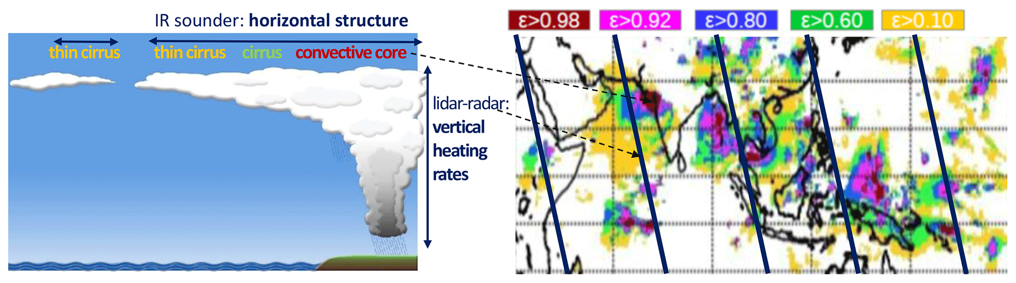
Figure 1Illustration of the three-dimensional cloud system concept, using space-borne IR Sounder data (AIRS), providing the horizontal component, and lidar–radar data (CALIPSO–CloudSat), providing the vertical component, both part of NASA's A-Train satellite constellation (left): based on two independent variables retrieved by AIRS, UT cloud systems are reconstructed from adjacent elements of similar cloud height (pcld); the horizontal emissivity structure allows the properties of convective cores (εcld>0.98) and cirrus anvils (right) to be directly linked. Clear-sky and low-level cloud fields are also identified (Fig. 4a of Protopapadaki et al., 2017). A horizontally complete picture of the vertical radiative heating rates will be obtained by laterally expanding them, as they are only available along narrow lidar–radar tracks (dark blue). Therefore we have developed optimized “non-linear regression models”, using deep neural network learning techniques, described in Sect. 2.4 and evaluated in Sect. 3, to relate the most suitable cloud and atmospheric properties from IR sounder and meteorological reanalyses to these heating rates.
A study by Li et al. (2013) finds that the column-integrated radiative heating of tropical UT clouds accounts for about 20 % of the latent heating. The radiative heating was estimated by combining International Satellite Cloud Climatology Project (ISCCP) data, classified as four distinct cloud regimes at a spatial resolution of 2.5∘ latitude and longitude, with heating rate profiles assigned from two tropical Atmospheric Radiation Measurement (ARM) sites, while the latent heating was deduced from measurements of the Tropical Rainfall Measuring Mission (TRMM) Precipitation Radar (PR). However, ISCCP and ARM data both may underestimate the effect of thin cirrus because its occurrence may be missed by ground observation (Protat et al., 2014) and by ISCCP (e.g. Stubenrauch et al., 2013), in particular when low-level clouds are also present and during the night.
Therefore, to include also the thinner cirrus and the complete 3D structure of these cloud systems, we applied a different strategy: to estimate the radiative heating rates of UT clouds we combined observations which are more sensitive to thin cirrus, together with machine learning techniques and a cloud system approach. The good spectral resolution of IR sounders makes them sensitive to cirrus, down to a visible optical depth of 0.2, during daytime and nighttime. Cloud properties retrieved from measurements of the cross-track scanning Atmospheric Infrared Sounder (AIRS) aboard the polar orbiting Aqua satellite have a large instantaneous horizontal coverage (Stubenrauch et al., 2017). They have been used by Protopapadaki et al. (2017) to reconstruct UT cloud systems. Recently these datasets have been extended, so that they now cover September 2002 to August 2019. On the other hand, the space-borne active lidar and radar measurements of the CALIPSO and CloudSat missions (Stephens et al., 2018a) supply the cloud vertical structure, in particular the radiative heating rates (Henderson et al., 2013). As this information is only available along successive narrow nadir tracks, separated by about 2500 km, we employed machine learning techniques on cloud, atmospheric and surface properties to build a 3D description of these cloud systems. These techniques were already successfully applied to extend IR brightness temperature (Kleynhans et al., 2017) and snow water (Snauffer et al., 2018) from other atmospheric variables.
This article presents the effect of UT clouds on tropical radiative heating rates in the longwave (LW) and shortwave (SW) spectral domain and the relationship between surface temperature, convective depth and anvil radiative heating and cooling. Section 2 describes the data which are used as input and target for the training of the neural networks, which themselves are also explained. Sensitivity studies and evaluation of these developed non-linear regression models are presented in Sect. 3. They give insight into the most appropriate cloud and atmospheric properties as well as into how many scene-dependent non-linear regression models are necessary to reliably predict the radiative heating rates of different cloud types. After application of these models to the 15-year time period of AIRS cloud data, combined with ERA-Interim atmospheric and surface data, Sect. 4 highlights results on the contribution of clouds, and in particular of MCSs, on the tropical radiative heating and cooling. Conclusions and an outlook are given in Sect. 5.
The different variables to be used for the prediction of the radiative heating rates are described in Sect. 2.1 and 2.2. Section 2.1 also presents cloud system data used in the analysis in Sect. 4. The target data are presented together with their uncertainties in Sect. 2.3. Finally the neural network construction is given in Sect. 2.4.
2.1 AIRS cloud data and cloud system data
Since 2002 AIRS (Chahine et al., 2006) aboard the National Aeronautics and Space Administration (NASA) Earth Observation Satellite Aqua has provided very high spectral resolution measurements of Earth emitted radiation in the thermal IR (3.74–15.40 µm) at 01:30 and 13:30 local time (LT). Cross-track scanning leads to a large instantaneous coverage of about 70 % in the tropics. The spatial resolution of these measurements at nadir is about 13.5 km.
The Clouds from IR Sounders (CIRS) data (Stubenrauch et al., 2017) provide cloud pressure (pcld) and cloud emissivity (εcld), as well as cloud temperature (Tcld) and cloud height (zcld), together with their uncertainties. The cloud retrieval is based on a weighted χ2 method (Stubenrauch et al., 1999), which uses eight channels along the 15 µm CO2 absorption band, with peak contributions between 235 hPa and near the surface. UT clouds are defined as clouds with pcld<440 hPa. They are further distinguished with respect to εcld as opaque high clouds (Cb, εcld≥0.98), cirrus (Ci, ) and thin cirrus (thin Ci, ). pcld is transformed to Tcld and zcld via the atmospheric temperature and water vapour profiles of ancillary data (see Sect. 2.2). An a posteriori multi-spectral cloud detection is based on the spectral coherence of retrieved cloud emissivity in the atmospheric window between 9 and 12 µm. This spectral region also provides information on the thermodynamic phase of the clouds, and for semi-transparent cirrus the slope of cloud emissivities between 9 and 12 µm gives an indication of the effective ice crystal diameter (Guignard et al., 2012). The CIRS cloud data are retrieved per AIRS footprint.
In order to obtain information on the surrounding cloud scene structure, 16 cloud regimes are distinguished by applying a k-means clustering on histograms of εcld and pcld within regions of 2∘ latitude × 2∘ longitude, similar to the method developed by Rossow et al. (2005) using ISCCP data. In addition, we provide the clear-sky fraction estimated from AIRS within these grid cells.
For the analysis in Sect. 4, we combine the resulting radiative heating rate fields with information on UT cloud systems. Their reconstruction is based on two independent variables, pcld and εcld (Protopapadaki et al., 2017): the AIRS cloud data were merged to grid cells of 0.5∘ latitude × 0.5∘ longitude, and then data gaps between adjacent orbits were filled. Only grid cells containing more than 70 % UT clouds were kept to reconstruct UT cloud systems from adjacent elements of similar cloud height, given by pcld. Convective cores, thick cirrus and thin cirrus within the anvils are identified by εcld intervals, with thresholds at 0.98 and 0.5. This cloud system concept is used in Sect. 4 to identify MCSs and to relate the radiative heating and cooling profiles of their convective cores and their anvils to different surface conditions. Therefore MSCs were defined as UT cloud systems with at least one convective core (built from grid cells with average εcld>0.98 within subregions of εcld>0.9).
2.2 Atmospheric and surface data
Atmospheric profiles as well as surface pressure and temperature are used as ancillary data for the CIRS retrieval. These values are provided by the ERA-Interim atmospheric reanalysis data of the European Centre for Medium-Range Weather Forecasts (ECMWF; Dee et al., 2011), given at a spatial resolution of 0.75∘ latitude × 0.75∘ longitude and four times per day. We interpolated the atmospheric profiles of temperature and water vapour to 23 pressure levels and derived the relative humidity within the 22 atmospheric layers from the temperature and water vapour profiles by a method based on Stubenrauch and Schumann (2005). The CIRS cloud retrieval classifies the atmospheric profiles by comparing them to about 2300 representative clear-sky atmospheric profiles of the Thermodynamic Initial Guess Retrieval (TIGR) database (Chédin et al., 2003), to choose the corresponding spectral atmospheric transmissivities for the radiative transfer in the retrieval. This atmospheric classification provides additional information for the non-linear regression models developed in Sect. 3.
For the prediction of LW heating rates over land we use spectral IR surface emissivities at wavelengths around 9.00, 10.16 and 12.18 µm, retrieved from IR Atmospheric Sounding Interferometer (IASI) measurements (Paul et al., 2012) and given as a monthly mean climatology at a spatial resolution of 0.25∘ × 0.25∘. Over water, the surface emissivity is set to 0.99 at 9 µm and to 0.98 at the two other wavelengths, according to Wu and Smith (1997).
For the prediction of the SW heating rates during daytime we use the visible surface albedo at noon local solar time and the solar zenith angle. The land surface albedos, retrieved from Moderate Resolution Imaging Spectroradiometer (MODIS) measurements (MODIS Collection 5, MOD43 product; Strahler et al., 1999), are distributed as a monthly climatology at a spatial resolution of 0.1∘ × 0.1∘ by the NASA Earth Observations (NEO) website (https://neo.sci.gsfc.nasa.gov/, last access: November 2019). Over ocean we assume a surface albedo at noon local solar time of 0.06.
In order to explore the benefit of adding the aerosol optical depth (AOD) to the input variables, we use a monthly climatology of AOD from MODIS (MODIS Collection 5, MOD04/MYD04 product; Levy et al., 2009) at a spatial resolution of 0.25∘ × 0.25∘, also distributed by the NEO website.
Finally we investigate the value of adding the vertical velocity at 500 hPa as an input variable, given at the spatial resolution of 0.375∘ × 0.375∘, from the ERA5 reanalysis (Hersbach et al., 2020).
2.3 CALIPSO–CloudSat vertical structure and collocation with AIRS
The vertical structure of the clouds can only be determined by active space-borne instruments. The Cloud-Aerosol Lidar with Orthogonal Polarization (CALIOP) aboard CALIPSO and the Cloud Profiling Radar (CPR) aboard CloudSat, both part of the A-Train constellation, follow AIRS within a few minutes. CALIOP provides backscatter profiles at a wavelength of 532 and 1064 nm. The backscatter ratio helps to distinguish between aerosols and clouds. The 94 GHz nadir-viewing CPR measures profiles of the power backscattered by clouds at a native vertical resolution of 480 m over footprints covering 1.8 km×1.4 km. By using oversampling, data are provided at a vertical resolution of 240 m. Combining information from both instruments allows for a complete description of the cloud vertical structure. However, this information is only given along successive nadir tracks.
We extended the collocated AIRS–CALIPSO–CloudSat data used by Feofilov et al. (2015) and Stubenrauch et al. (2017) by the NASA 2B FLXHR-LIDAR (R04) heating rates for the period of 2007 to 2010. These vertical profiles have about 80 values over a height of 20 km. Since the AIRS cloud height is retrieved as pressure and the input parameters are not precise enough to predict such a fine vertical structure, we transformed the FLXHR-LIDAR heating rates to 22 pressure layers between 70 hPa and the surface. For each of the AIRS footprints this collocated dataset also includes the number of detected cloud layers, from the 2B-GEOPROF-LIDAR data, used in Sect. 3 to evaluate the clear-sky identification by AIRS alone.
The radiative fluxes and heating rates of 2B-FLXHR-LIDAR (version R04; Henderson et al., 2013; L'Ecuyer et al., 2008) were derived by applying the BUGSrad broadband radiative transfer model (Ritter and Geleyn, 1992) to the scenes observed by CALIPSO–CloudSat, using as inputs the vertical location of the cloud layers (2B-GEOPROF-LIDAR; Mace et al., 2009), the cloud water/ice content and effective particle sizes retrieved from radar only (2B-CWC-RO; Austin et al., 2009), distinction between cloud and rain water contents from 2C-PRECIP-COLUMN (Haynes et al., 2009) and collocated atmospheric and surface auxiliary data from ECMWF. For the clouds and aerosols which are undetected by CloudSat, the MODIS-based cloud optical depth (2B-TAU) and CALIPSO version-3 products (Winker et al., 2010) are used to calculate the corresponding radiative properties. The phase of thin clouds only detected by CALIPSO is set to ice for T<253.15 K, and their ice crystal equivalent mass sphere effective radius is assumed to be 30 µm.
The comparison of 2B-FLXHR-LIDAR (R04) with CERES–CALIPSO–CloudSat–MODIS (CCCM) products, using a finer vertical resolution and different microphysics than FLXHR-LIDAR, revealed a small low bias in SW heating of FLXHR-LIDAR due to a slight underestimation of cloud occurrence of height below 1 km, while the LW heating of CCCM for thin cirrus is slightly larger (Ham et al., 2017).
Over the tropical ARM site of Darwin, Protat et al. (2014) found a good agreement between the shapes of the 2B-FLXHR-LIDAR radiative heating rates and those derived from ground-based remote sensing (Mather et al., 2007) and from an experimental 2C-ICE-FLUX product for altitudes between 1 and 12 km. Above 12 km, in comparison to 2B-FLXHR-LIDAR, the underreported cirrus frequency by the ground-based lidar leads to a negative bias of 0.4 to 0.8 K d−1 in the LW heating rates, whereas different microphysical properties of thin cirrus in 2C-ICE-FLUX produce about 0.3 K d−1 larger LW heating rates. The same 2C-ICE microphysical properties (Deng et al., 2013), together with improved cloud phase identification and surface characteristics, are integrated in the very recently released version R05 of FLXHR-LIDAR data (Matus and L'Ecuyer, 2017). The improvements lead to a slightly better agreement with top of atmosphere (TOA) fluxes from the Clouds and the Earth's Radiant Energy System (CERES), and the global annual mean atmospheric cloud radiative effect between both versions differs by about 10 % (Hang et al., 2019): 7.8 W m−2 (R05) compared to 8.6 W m−2 (R04). As version R05 of the FLXHR-LIDAR data was only released when we were finishing our analyses of Sect. 4, we present the results which used 2B-FLXHR-LIDAR (R04) data for the training of the artificial neural networks (ANNs), keeping in mind that the cirrus heating rates (HRs) above a height corresponding to 200 hPa are more reliable than those from ground-based measurements but may be still slightly underestimated compared to newer versions with different ice microphysics (Protat et al., 2014; Ham et al., 2017; Hang et al., 2019). Within the overall uncertainties described in this section and in Sect. 3, the results in Sect. 4 are still valid.
2.4 Artificial neural network construction
The challenge in creating a complete 3D description of the UT cloud systems and their environment lies in the lateral expansion of the information on the vertical structure, only available at the locations sampled along the lidar–radar nadir tracks. Figure 1 illustrates the collocation of vertical heating rates deduced from lidar–radar along these tracks and horizontal cloud information from IR sounders. In order to achieve our goal of creating complete 3D heating rate fields, we developed nonlinear regression models based on ANNs which use as input the combined AIRS and ERA-Interim data described in Sect. 2.1 and 2.2. ANNs have seen spectacular progress during the last few years, especially in the automation of finding the most appropriate weights used in the ANN layers. We used the TensorFlow framework (https://www.tensorflow.org/, last access: January 2019) to train machine learning models with the help of the Keras program library (https://keras.io/, last access: November 2019) for Python, with training and testing along the nadir tracks. The 4 years of collocated data correspond to a very large statistics of more than 16 million data points. When developing scene-type-dependent models in Sect. 3.2, samples vary from 4.8 million data points for mid- and low-level clouds over ocean to 94 000 data points for Cb over land.
Kleynhans et al. (2017) demonstrated that thermal IR radiation at top of atmosphere, measured by MODIS, can be best simulated from available atmospheric reanalysis data by using a multi-layer perceptron (MLP)-supervised learning technique. This technique produced the lowest overall error rates, in particular over cloudy situations, compared to non-linear support vector regression (SVR), convolutional neural network (CNN) and even to atmospheric radiative transfer simulations.
After having tested the MLP performance on the number of hidden layers within the ANN, our final ANN consists of an input layer with the approximately 30 to 45 input variables (see Sect. 3), two hidden layers with 64 neurons and an output layer which corresponds to the radiative heating rates given in 22 pressure layers. To improve the performance, we used the rectified linear unit (ReLU) layer activation function. For a better efficiency we use the Adaptive Moment Estimation (Adam) optimizer, using adaptive learning rates (Kingma and Ba, 2017).
The training dataset is randomly separated into three portions: 80 % are used for training, 10 % for validation and 10 % for testing. In order to have similar cloud type, day–night and ocean–land statistics in these portions, we stratified the data by cloud type, ocean–land and day–night for LW and by cloud type and ocean–land for SW (only available during daytime). The model parameters are fitted by minimizing a loss function, which corresponds to the average of the squared differences between the predicted heating rates and the target values from the lidar–radar observations of the 22 pressure layers. For the determination of the quality of the resulting regression models we use then as metrics the average of the 22 mean absolute errors (MAEs) between the prediction values and the target values. In order to avoid overfitting, we stop the fitting when the minimum loss does not further improve during 10 iterations (epochs).
As many input variable distributions are not Gaussian, and to avoid outliers, we normalized the input variables by subtracting an “acceptable” minimum and then dividing by the difference between the “acceptable” variable maximum and minimum. These acceptable minimum and maximum values have been established for each variable and adapted to the scenes for which the models were trained: ocean or land, all cloud types, clear sky, high clouds or mid- and low-level clouds. Before the application of the model, all input variables are first bounded between these minimum and maximum values.
We assessed the sensitivity of the predicted radiative heating rates (HRs) to the selection of input variables (Sect. 3.1). In general, a model trained over all clouds over ocean and land together smoothes out differences between different cloud types and between ocean and land. Furthermore scenes which are less frequent may have a smaller weight and may be therefore less represented than other scenes. Since we are interested in the study of the effect of UT cloud systems, we chose to develop separate MLP ANN models for
- 1.
Cb
- 2.
Ci and thin Ci
- 3.
mid- and low-level clouds
- 4.
clear sky,
each separately over ocean and over land, leading to eight models. Comparisons of these models with those developed for all clouds together are on average small and are described in the Supplement, while the evaluation of the final eight models is given in Sect. 3.2. The cloud and clear-sky models were then combined to construct the radiative HRs over the whole tropical band (Sect. 3.3).
3.1 Sensitivity to input variables
The input variables describing the cloud, atmosphere and surface properties used for the prediction of the radiative HRs are summarized in Table 1.
The training for the SW HRs is based only on data recorded at 13:30 LT, while the training for the LW HRs exploits data for both 01:30 and 13:30 LT. Since the CALIPSO data are slightly more sensitive during night-time, we used for the LW training a day–night flag as an additional input variable. The choice of input variables slightly differs for the prediction of LW and SW HRs: for the training of LW HRs, we used surface spectral IR emissivities, while for the training of SW HRs, we used surface albedo and solar zenith angle.
The MLP regression models compute radiative HRs for 22 pressure layers from 70 to 1000 hPa, using about 40 input variables. Earth topography implies that the temperature, relative humidity and radiative HR profiles are not always determined over all 22 pressure layers. Given that neural networks need a constant number of input and output values, we had to replace the missing values below the surface. Therefore, we first continued the temperature, relative humidity and radiative HR profiles below psurf with their lowest valid value and then added to these values the average vertical gradients between the corresponding layer and the layer with the lowest valid value. These gradients were computed using the average profiles of regions containing all 22 pressure layers, separately determined over ocean and over land, and per cloud type and month. Even if these values below the surface are not used in the analyses, they slightly influence the training.
For the sensitivity study of the most appropriate variables (Table 1), we considered cloudy scenes over ocean, and we set up six different experiments to predict the LW (SW) HRs, starting with
- 1.
a set of 18 (19) basic variables, which describe cloud, atmospheric and surface properties: CIRS cloud properties and their uncertainties, cloud spectral emissivity difference between 9 and 12 µm, AIRS brightness temperatures, total precipitable water, tropopause height and TIGR atmosphere class, and surface pressure and temperature.
Then we gradually added to the basic variables of experiment 1:
- 2.
cloud regime classification and its uncertainty given by the kernel distance: total of 20 (21) input variables;
- 3.
relative humidity in 10 layers: total of 30 (31) input variables;
- 4.
atmospheric temperature in 10 layers: total of 40 (41) input variables;
- 5.
vertical velocity from ERA5 reanalyses: total of 41 (42) input variables; and
- 6.
monthly mean aerosol optical depth: total of 42 (43) input variables.
Table 1List of input variables for the prediction of LW and SW heating rates and sensitivity experiments.
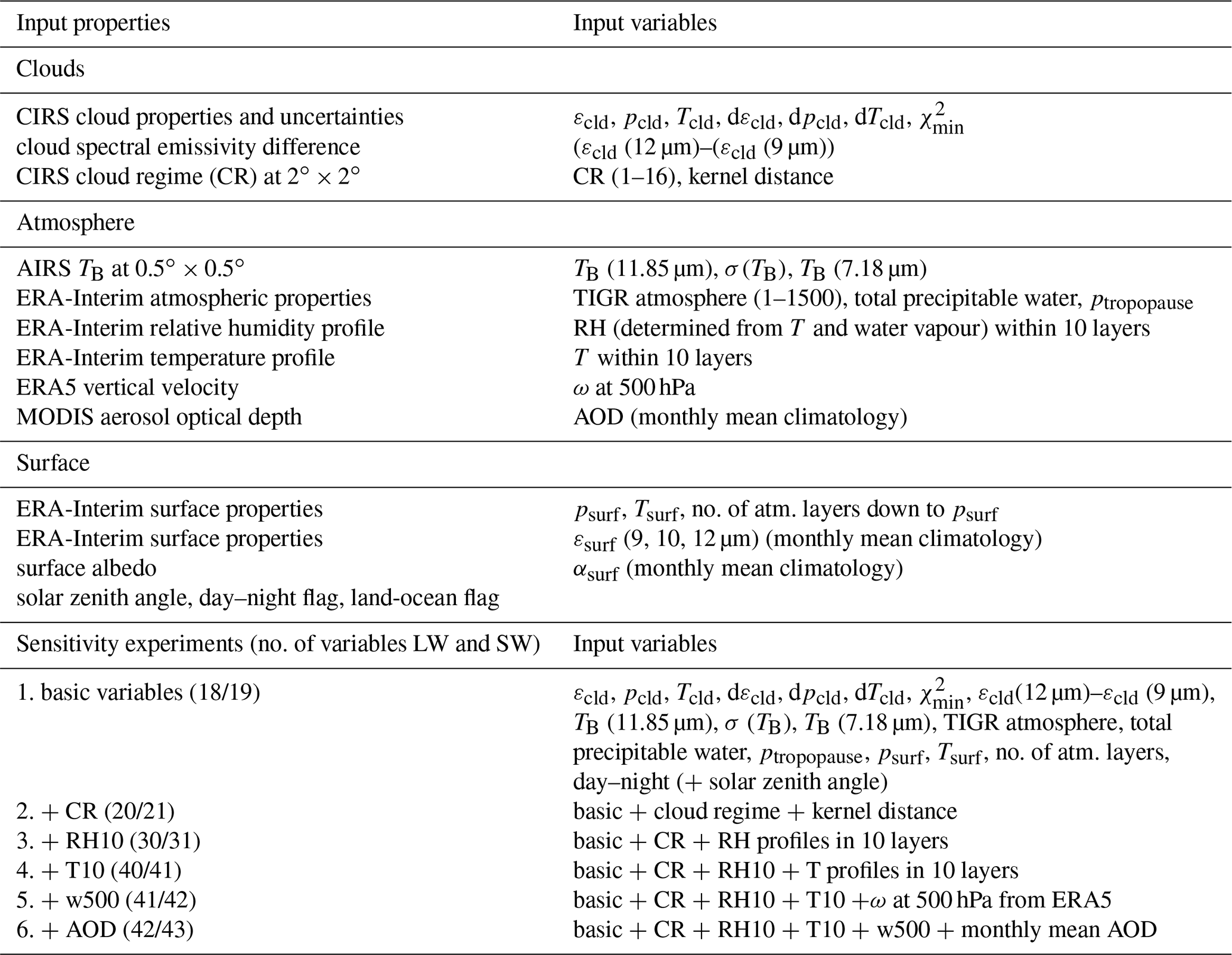
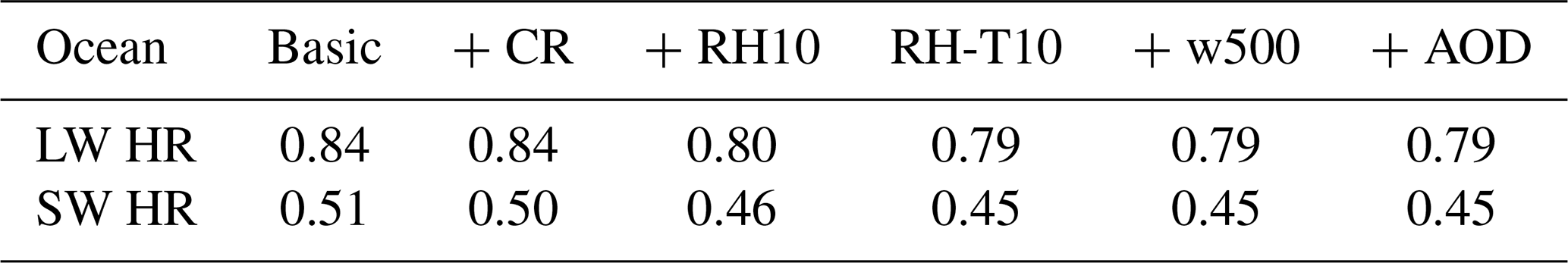
Table 2 compares the mean absolute error (MAE) for the prediction of LW and SW heating rates of clouds over ocean from the experiments 1 to 6. In all cases the MAEs over the validation data and over the testing data are within 0.01 K d−1. The MAE over the testing dataset is shown. The similarity in MAE between the validation and testing data means that there is no underfitting (the variables are not sufficient to predict the target) nor overfitting (the model is too detailed, with too many variables or the database is not sufficiently large). As shown in Table 2, the MAE decreases by about 5 % (10 %) for the LW (SW) model when the atmospheric profiles are included. The addition of vertical velocity and of AOD do not seem to improve the results. This lack of improvement may be explained by noise coming from these sources in combination with the AIRS cloud properties and ERA-Interim atmospheric and surface properties. The addition of the temperature profile only slightly improves the prediction of the heating rates, most probably because the atmospheric T profiles are more similar within the tropics than the atmospheric relative humidity profiles.
Table 2MAE (K per day) for the prediction of LW or SW heating rates of clouds over ocean, from experiments 1–6.
As the MAE only provides an average estimation of the quality of the prediction, we also considered the difference between the predicted radiative HRs and those determined from CALIPSO–CloudSat measurements over tropical ocean, separately for Cb, Ci, thin Ci and mid-level and low-level clouds. The LW and SW results of the different experiments, using the testing dataset, are compared in Fig. 2. Overall, all results show good agreement between predicted and CALIPSO–CloudSat-derived HRs. The differences between mean predicted and “observed” radiative HRs undulate well around 0 K d−1. However, we note that when using the ERA5 vertical velocity at 500 hPa as an additional input variable, the results for Cb and mid- and low-level clouds in the LW are slightly degraded. Similarly, the addition of the monthly mean AOD does not improve the results. This indicates only a medium compatibility between these two variables and the instantaneous AIRS cloud properties and ERA-Interim atmospheric and surface properties. Therefore we use in the following the input variables of experiment 4 for the model development. The 30 % quantiles and 70 % quantiles of the HR differences in Fig. 2 give an indication of the uncertainty, which may be related to differences in horizontal resolution between AIRS and CALIPSO–CloudSat. In particular for convective towers of very large optical depth (Cb) and for mid- and low-level clouds, the coarse AIRS spatial resolution may lead to a mixture of several cloud types or of clouds and clear sky within one footprint.
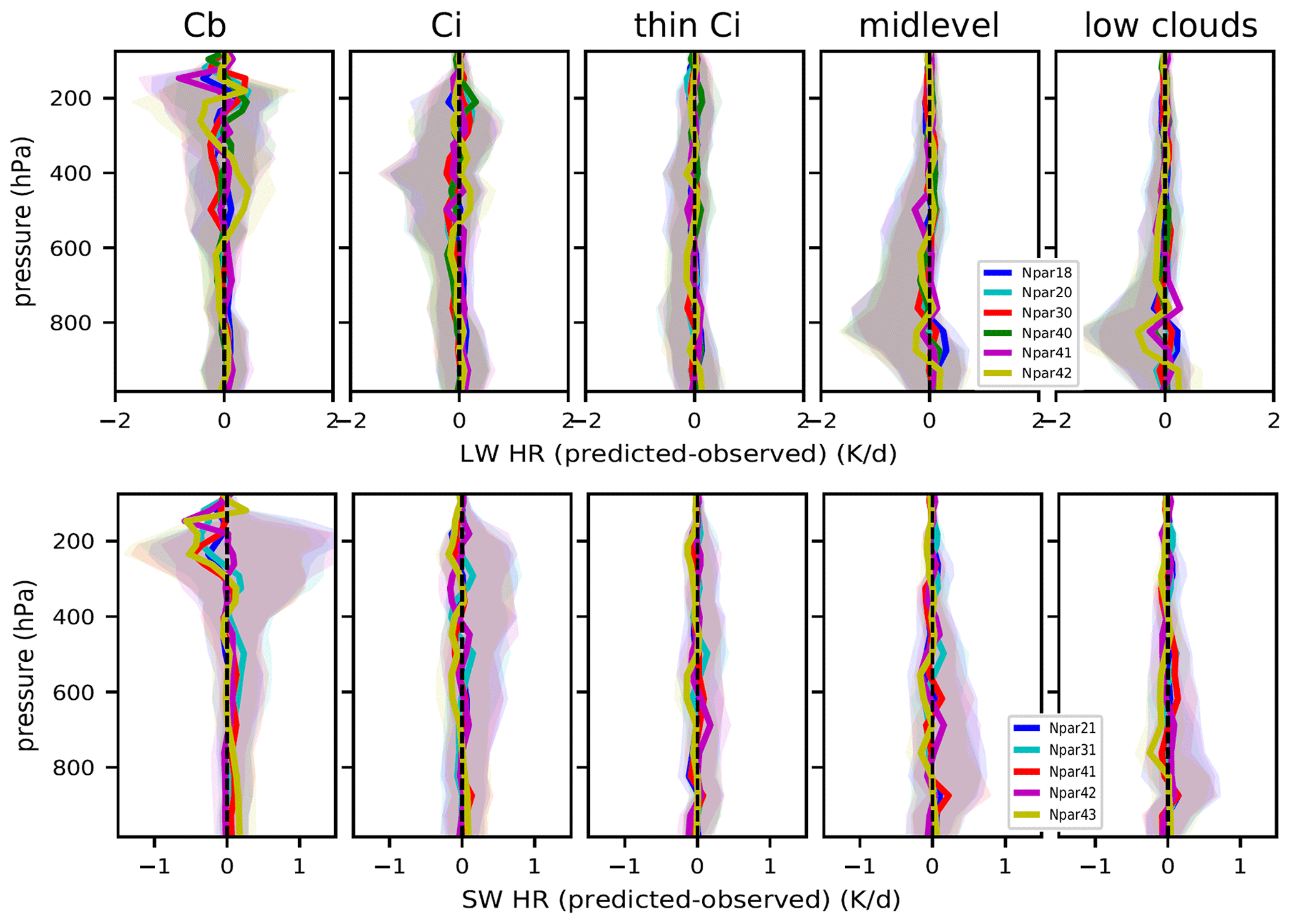
Figure 2Sensitivity results concerning surface, atmospheric and cloud input parameters for the prediction of cloud LW radiative heating rates (above) and SW radiative heating rates (below): difference between predicted and observed vertical profiles of the validation dataset, separately for Cb, cirrus, thin cirrus and mid- and low-level clouds, as identified by AIRS-CIRS, over tropical ocean. 30 % and 70 % quantiles of the distributions are also shown. Compared are results of the experiments 1–6 (above) and 2–6 (below), using the input parameters listed in Table 1.
Furthermore, the radiative HRs also depend on the cloud vertical extent and the number of vertical cloud layers, which are not explicitly given in the input data. However, cloud emissivity and cloud vertical extent are well related (Fig. 10 of Stubenrauch et al., 2010), as well as cloud vertical extent and the number of vertical cloud layers (e.g. Wang et al., 2000).
Considering the radiative HR profiles of the different cloud types shown in Fig. 3, constructed for 1 month of data over the whole tropical band (see Sect. 3.3), we find that the largest uncertainties for the relatively high opaque clouds (Cb and Ci) are around the maxima of LW cooling and SW heating which correspond to approximately 15 % to 25 %. The variability in the vertical profiles of microphysical properties within these clouds which may not be reproduced by the input variables is certainly another cause for these uncertainties.
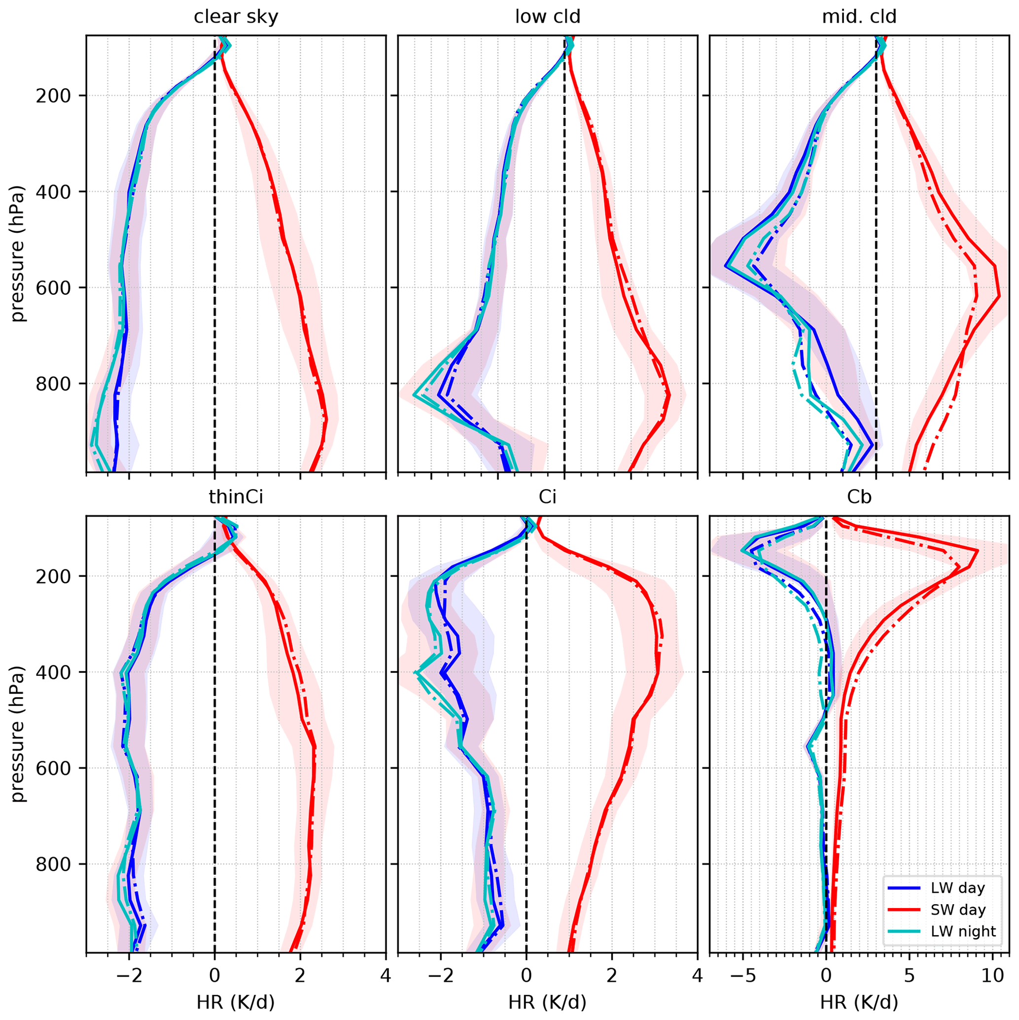
Figure 3Predicted LW heating rates and SW heating rates (full line), separately for clear sky, low- and mid-level clouds, thin cirrus, Ci and Cb, as identified by AIRS-CIRS, averaged over the AIRS swaths within 30∘ N–30∘ S, in January 2008. 30 % and 70 % quantiles of the distributions indicate their variability. The model has been trained individually over Cb, Ci/thin Ci and mid- and low-level clouds, separately over ocean and land. Broken lines correspond to the average of FLXHR heating rates averaged along the CALIPSO–CloudSat nadir tracks. Night corresponds to 01:30 LT and day to 13:30 LT.
3.2 Scenes used for the training
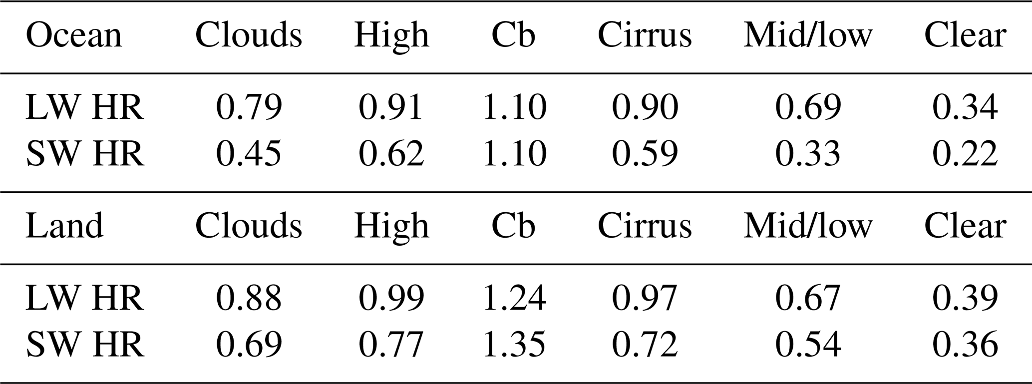
When using one model for all clouds over ocean and land, the MAE is 0.82 K d−1 for LW and 0.51 K d−1 for SW HRs. Table 3 presents the MAE for the prediction of LW and SW HRs over the testing data, separately for different scene types over ocean and over land. In general, the performance is slightly better over ocean than over land, which can be explained by a greater homogeneity of surface, in particular in the SW, and atmospheric properties. We also observe a decreasing performance from clear-sky scenes (LW 0.36 K d−1 and SW 0.27 K d−1) over mid- and low-level clouds towards high-level clouds and Cb, which again can be explained by an increasing inhomogeneity, and in the case of Cb the saturation of εcld at 1.
Table 3MAE (K per day) for the prediction of LW and SW heating rates using models over different scene types.
We also estimated the uncertainty of the final eight scene-dependent ANN models after having them applied to 1 month of AIRS data, over the whole tropical band. Regional differences in three atmospheric layers (106–131, 200–223, 525–585 hPa) between predicted LW HRs obtained from these models and those from models developed over all clouds, separately over ocean and over land, lie generally within 0.25 K d−1, with only a few regions of 0.45 K d−1 (Fig. S5 in the Supplement), keeping in mind that the more detailed cloud type distinction will give the better results.
3.3 Construction of tropical heating rate fields
After applying the final eight scene-dependent ANN models to 1 month of AIRS data, over the whole tropical band (30∘ N–30∘ S) and averaging the resulting radiative HRs at a spatial resolution of 0.5∘ latitude × 0.5∘ longitude, we compare the averages of these laterally extended LW and SW HRs with those of FLXHR (along the nadir tracks), separately for clear sky and for five cloud types (Cb, Ci, thin Ci, mid-level and low-level clouds). Averages of predicted and “observed” radiative HRs in Fig. 3 are very similar, despite different sampling and spatial resolution. This means that the nadir track statistics gives a good picture of the monthly average over the whole tropics and that the prediction models provide on average reliable results. The 30 % and 70 % quantiles of the distributions indicate variabilities for clear sky and thin cirrus. The larger variabilities for the more opaque clouds are related to their monthly variability in height, optical depth and vertical extent. The relatively large variability for mid-level clouds, with an occurrence in the tropics of about 6 %, may be related to the fact that these are often situated in regions with a mixture of different cloud types. The LW HRs are very similar during the day and night, and the presented cloud-type-dependent radiative heating rates agree well with earlier publications (e.g. Oreopoulos et al., 2016).
In a clear-sky situation, LW cooling occurs, linked to the absorbed and transmitted energy by the molecules in the atmosphere. As shown in Fig. 3, this cooling lies between −2.5 and −2 K d−1 within the troposphere up to 200 hPa, where it decreases rapidly until it reaches about 0 K d−1 around 100 hPa. Since the AIRS clear-sky identification may also include subvisible cirrus as well as partly cloudy scenes within the AIRS footprint, we estimated how much this affects the radiative HRs by comparing the FLXHR HRs for AIRS clear-sky and for CALIPSO–CloudSat clear-sky identification (Fig. S6). Definitely, there is a slight positive bias in the clear-sky LW heating near 100 hPa of about 0.1 to 0.2 K d−1 due to subvisible cirrus, in particular during the night, when the CALIPSO lidar better detects subvisible cirrus. The small SW clear-sky heating positive bias of the same order of magnitude between 400 and 800 hPa is most probably linked to contamination by partial cloudiness.
Clouds introduce sharp vertical gradients to this LW cooling: relatively opaque clouds heat the atmospheric column below by trapping surface emissions but cool the column above due to excess emission, while thin cirrus heat the UT by intercepting the LW radiation coming from below. Indeed, Fig. 3 exhibits a LW cooling above optically thick clouds, the strongest effect above Cb, of about −4.5 K d−1 around 170 hPa, and a heating within the clouds and below the clouds, compared to clear sky. The small cooling around 550 hPa is due to melting, owing to the transition from ice to liquid phase which occurs at or just below the freezing level at about 5 km altitude throughout the tropics, and the different emissivities of liquid and ice cause a flux divergence at that level (Tristan L'Ecuyer, personal communication, 2017). The cooling above mid- and low-level clouds is located around 600 and 800 hPa, respectively. Thin cirrus heat the UT around 100 hPa.
During day in the SW range, the sunlight heats the atmosphere and the particles within the cloud. Figure 3 shows a strong heating in the upper part of the Cb with a maximum of about 8 K d−1 around 200 hPa, while in the rest of the cloud this effect is negligible, given that the sun is blocked by the dense cloud particles. For mid-level clouds a small peak is found around 600 hPa and for low-level clouds around 850 hPa.
In order to illustrate the additional value of the lateral expansion of the radiative HRs, Fig. 4 presents geographical maps of mean LW heating and cooling in four specific pressure layers (around 106, 200, 525 and 850 hPa, respectively) for January 2008, compared to the monthly mean nadir track statistics from CALIPSO–CloudSat. These four pressure layers were chosen according to (1) UT heating by thin cirrus, (2) cooling above Cb and thick cirrus, (3) middle troposphere heating by high thick clouds and (4) cooling above low-level clouds and a heating below clouds. The horizontal structures of the predicted HR fields agree quite well with those from FLXHR, but they appear clearer, since the spare nadir track statistics is quite noisy.

Figure 4Geographical maps of LW heating rates (K per day) in four layers: 106–131, 200–223, 525–585 and 850–900 hPa (from top to bottom) averaged over January 2008 at 01:30 LT. Left: predicted over the AIRS swath, using the combination of the eight models developed for Cb, Ci/thin Ci, mid- and low-level clouds and clear sky, separately over ocean and over land. Right: from NASA FLXHR data along the CALIPSO–CloudSat nadir tracks.
By using the 3D radiative heating fields constructed in Sect. 3, we first quantify the effect of tropical clouds on the atmospheric radiative cooling, in comparison to earlier results (Sect. 4.1). In Sect. 4.2 we use the cloud system approach described in Sect. 2.1 to study the heating and cooling within convective cloud systems by distinguishing convective cores (Cb), cirrus anvil (Ci) and surrounding thin cirrus (thin Ci), comparing warm and cool tropical ocean. Finally, we investigate tropical heating changes with respect to variations of tropical surface temperature, climate indices and cloud properties (Sect. 4.3).
4.1 Tropics-wide cloud radiative heating
As seen in Fig. 3, clouds introduce sharp vertical gradients to the atmospheric radiative cooling profile, and we are in particular interested in the effect of UT clouds and MCSs. Li et al. (2013) have found that the tropics-wide 24 h mean UT cloud radiative heating effect has a narrow maximum of about 0.45 K d−1 around 250 hPa and that the column-integrated radiative heating of UT clouds accounts for about 20 % of the latent heating estimated by TRMM, the latter with a broad peak of about 1.7 K d−1 around 450 hPa. These results were obtained by using radiative heating rates calculated from ground-based lidar and radar measurements at two ARM sites (Manus and Darwin), classified by ISCCP UT cloud regimes and then expanded over the deep tropics according to the ISCCP UT cloud regime occurrence frequency.
In order to compare our results to this significant result, we concentrate on the same latitude band from 15∘ N to 15∘ S, and we calculate the 24 h SW heating rates by multiplying the SW heating rates at 13:30 LT by , where Θ is the solar zenith angle. The latter is about 33∘ near the Equator. Similar to the HR normalization of Li et al. (2013), we neglect seasonal and geographical variations. The cloud radiative heating effect (CRE) is determined as the difference between cloud HR and clear-sky HR, weighted by total cloud amount, and for the CRE of a specific cloud type, additionally weighted by its relative amount of specific cloud type. The net CRE is then the sum of the LW CRE, averaged over 01:30 and 13:30 LT, and the 24 h SW CRE using the HRs at 13:30 LT, weighted by , and the sum weighted by the specific cloud amounts averaged over 01:30 and 13:30 LT. This estimation assumes that the daily average of cloudiness can be estimated by the values 01:30 and 13:30 LT. Indeed, the diurnal variation of UT cloud cover over tropical ocean determined from four daily observations is less than 2 % and reaches about 7 % over tropical land (Feofilov and Stubenrauch, 2019), with slightly less cirrus and thin cirrus at 13:30 than at 01:30 LT.
Total tropical cloud cover is 60 %, varying between 57 % at 13:30 LT and 63 % at 01:30 LT. We find that 55 % of these clouds are UT clouds, and 45 % are single-layer mid- or low-level clouds. Figure 5 presents a tropics-wide 24 h mean radiative heating induced by mid- and low-level clouds and by UT clouds. The CRE of UT clouds is further distinguished into the CRE of MCSs and of thin cirrus and furthermore of thin cirrus associated with MCSs, which are about half of all thin cirrus.
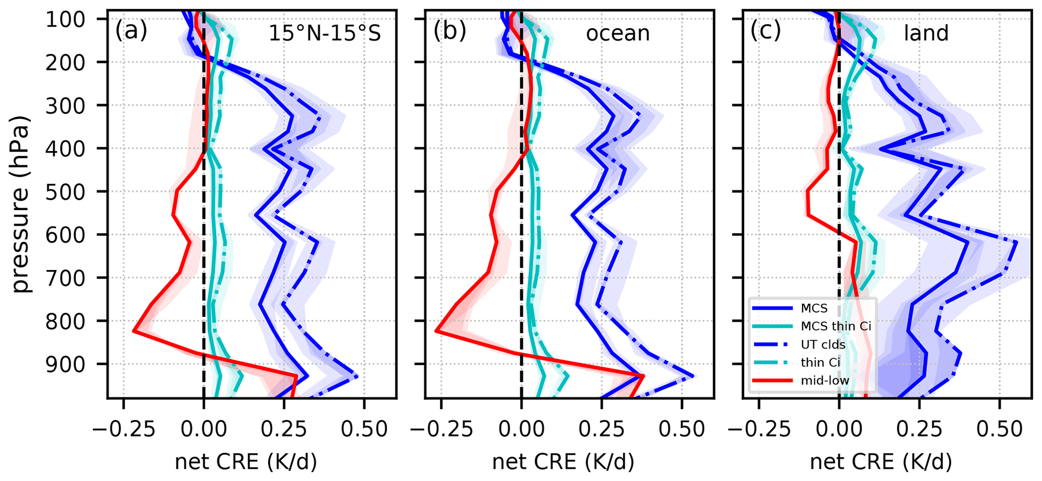
Figure 5Tropical mean net radiative heating effect within the troposphere of low- and mid-level clouds (red) and UT clouds (broken blue line), for the latter the effect of MCSs (blue), thin cirrus surrounding MCSs (cyan, full line) and all thin cirrus (broken cyan line) is shown separately. (a) All, (b) ocean and (c) land. Cloud observations averaged over 01:30 and 13:30 LT, with SW radiation normalized to 24 h, similar to Li et al. (2013). Statistics of 15 years (2004–2018), averaged over 15∘ N to 15∘ S. The sum of UT cloud and mid- and low-level cloud contributions corresponds to the total cloud heating effect, defined as the difference between total and clear-sky heating.
According to Fig. 5, the tropics-wide 24 h mean CRE of UT clouds is about 0.3 K d−1 from 250 hPa downward throughout the troposphere. The heating decreases towards 0 K d−1 at 200 hPa, and above this altitude a small net cooling is observed. Uncertainties related to cloud cover uncertainty and to clear-sky identification are also indicated. They have been determined by using the cloud amount at 01:30 LT with the HRs at 13:30 LT and by subtracting the CIRS clear-sky identification HR bias (Fig. S6). They are small in the lower troposphere, except over land, while they reach up to 0.08 K d−1 between 450 and 300 hPa.
The CRE values are in the same range as the ones determined by Li et al. (2013). However, the vertical shape of the CRE is significantly different: whereas the earlier result shows a narrow maximum of 0.45 K d−1 around 250 hPa and a minimum heating of about 0.1 K d−1 around 800 hPa, our estimation indicates a much more vertically extended heating effect of 0.3 K d−1 from 250 hPa downward throughout the troposphere. Compared to Fig. 9 of Li et al. (2013), the reinforcement of the latent heating is therefore vertically different, with a larger contribution between 800 and 330 hPa (Fig. S6). The enhancement factor between our column-integrated radiative heating of UT clouds and this latent heating (between 100 and 900 hPa) lies between 20 % and 25 %, very similar to and with a slightly larger upper limit than 21 % found by Li et al. (2013).
The difference in the profile shape of the UT cloud radiative heating effect is not related to the exploitation of profiles from only two ARM sites, since the profiles averaged over both sites are similar to the ones averaged over the whole tropics (not shown). However, as discussed by Protat et al. (2014), a significant portion of the ice cloud observations using ground-based measurements is attenuated by any liquid cloud below ice clouds or by the liquid part of deep convective systems. This yields a smaller SW heating than the satellite estimates in the middle troposphere. Another key reason for an underestimation of the CRE in the lower troposphere is that the ISCCP cloud regimes have been determined at a spatial resolution of 2.5∘, and especially the cirrus and mixed cloud regimes, which are the most frequent out of the four UT cloud regimes (72 %), include also a certain fraction of single-layer low-level clouds next to the cirrus clouds. When considering the radiative effect of mid- and low-level clouds in Fig. 5, which shows a cooling in the middle and lower troposphere down to 880 hPa, the shape of the radiative heating profile contribution of the ISCCP UT cloud regimes can be explained by the fact that at the coarse spatial resolution of 2.5∘, the UT cloud regimes also contain surrounding single-layer low-level clouds. In addition, the identification of thin cirrus with optical depth less than 1.3, the most frequent within these two ISCCP cloud regimes, is also less reliable, and the cloud height in this case is often just set to the tropopause height (e.g. Stubenrauch et al., 2012).
Further consideration of Fig. 5 shows that MCSs considerably contribute to the UT CRE. The UT cooling above the opaque parts of the MCSs is compensated for by thin cirrus UT heating, with half of the effect coming from those directly surrounding the anvil and the other half from in situ cirrus. The average net radiative heating within and the cooling above the MCSs seem to be slightly stronger over ocean than over land. Mid- and low-level clouds present a cooling above the clouds and a heating within and below. Since there are more low-level clouds over ocean and more mid-level clouds over land, the shapes of the net CRE differ accordingly. The HR profiles of UT clouds, initially deduced from CALIPSO–CloudSat data, include the effect of lower clouds underneath, as the warming peaks around 920 hPa over ocean and around 650 hPa over land suggest.
From Fig. 6, which compares the tropics-wide mean net radiative heating effect of the different cloud types at 01:30 and at 13:30 LT, we deduce a large difference in the profile shapes between nighttime and daytime and therefore in their vertical heating gradients. During nighttime, UT clouds heat the troposphere from 300 hPa downward increasingly, with a maximum of about 0.6 K d−1 around 920 hPa. The thicker UT clouds lead to an average cooling, with a minimum of −0.25 K d−1 around 200 hPa, which leads to a strong vertical gradient. The heating of the lower troposphere is slightly larger over land but with a smaller vertical gradient in the lower troposphere. Thin cirrus show a small average heating effect around 150 hPa, slightly larger over land than over ocean. During daytime, with additional solar heating, UT clouds, in particular the thicker ones, are strongly heated (see also Fig. 3), which leads to a tropics-wide maximum of about 0.6 K d−1 between 250 and 350 hPa. The heating strongly decreases towards the lower troposphere. Again, most of the effect of UT clouds can be explained by MCSs (as both are close to each other).
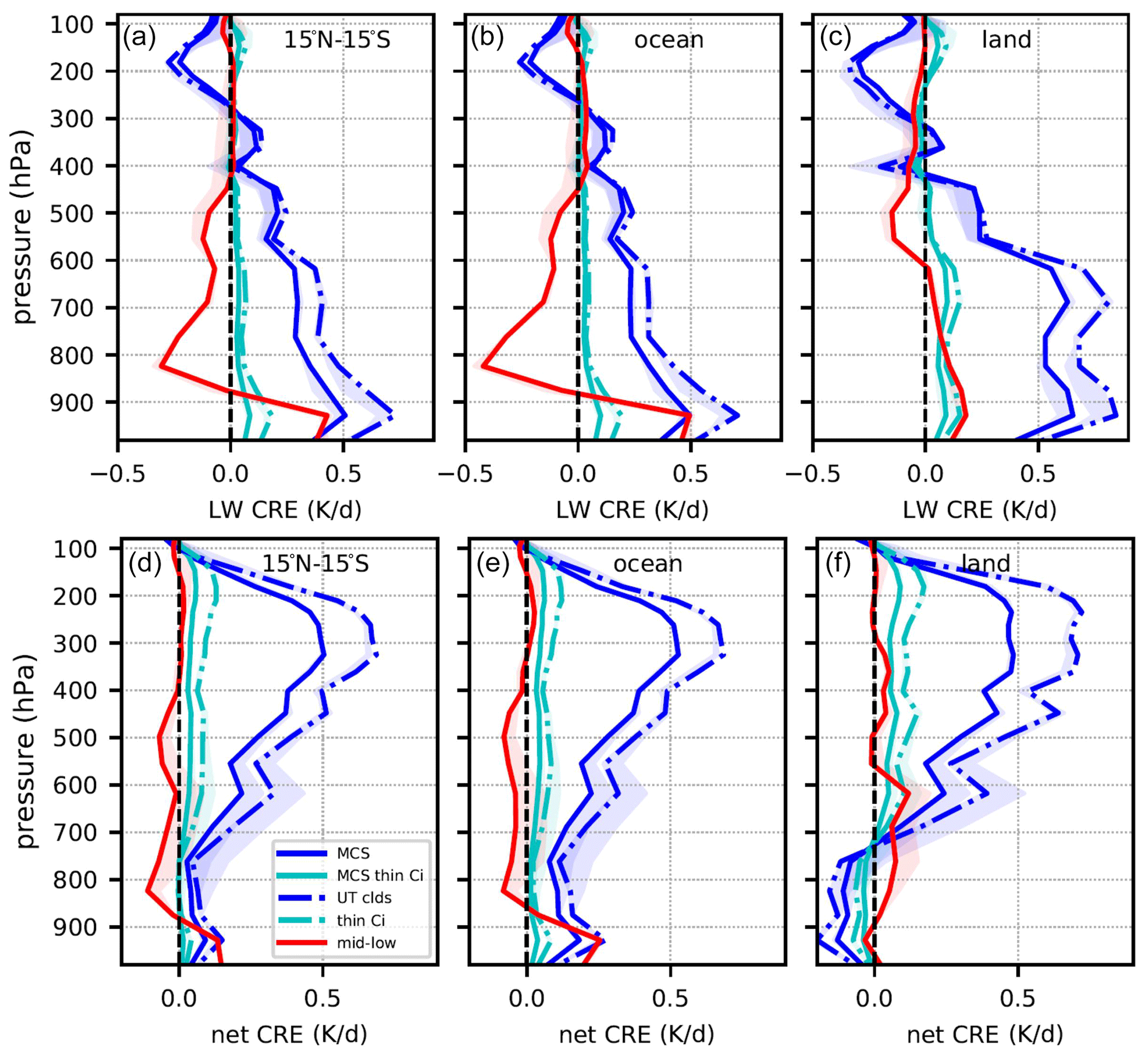
Figure 6Tropical mean net radiative heating effect within the troposphere of low- and mid-level clouds (red) and UT clouds (broken blue line); for the latter the effect of MCSs (blue), thin cirrus surrounding MCSs (cyan, full line) and all thin cirrus (broken cyan line) is shown separately. (a, b) All, (c, d) ocean and (e, f) land. Above: at 01:30 LT, below: at 13:30 LT. Statistics of 15 years (2004–2018), averaged over 15∘ N to 15∘ S.
During nighttime and during daytime, thin cirrus have on average a small heating effect throughout the whole troposphere. The effect of low-level and mid-level clouds differs diurnally: during nighttime they cool the atmosphere above their top, leading to peaks of −0.3 K d−1 around 820 hPa and of −0.1 K d−1 around 550 hPa, respectively, and they heat below, while during daytime the SW contribution partly compensates for these effects. In general, the UT cloud effect is a strong heating of the UT during daytime and a strong lower tropospheric heating during nighttime, leading to opposite vertical gradients.
Finally, Fig. 7 presents geographical maps of precipitable water, surface temperature and frequency of occurrence of UT cloud systems, as well as the 24 h net CRE, averaged over the whole period of 15 years, in three vertical layers: integrated over 106 to 200 hPa, over 200 to 585 hPa and over 585 to 900 hPa. UT clouds are most frequent over the western Pacific Ocean, including Indonesia, over the Amazon region and over central Africa. These are also the moistest regions. In the uppermost layer we observe horizontal structures linked to thin cirrus heating (red) and to cooling above the thicker parts of the MCSs (blue), whereas regions of clear sky or single-layer low-level clouds are in between (yellow to green). Over the western Pacific, the layers underneath are heated by the MCSs, while other regions are cooled just above lower clouds. The horizontal structures agree qualitatively with L'Ecuyer and McGarragh (2010).
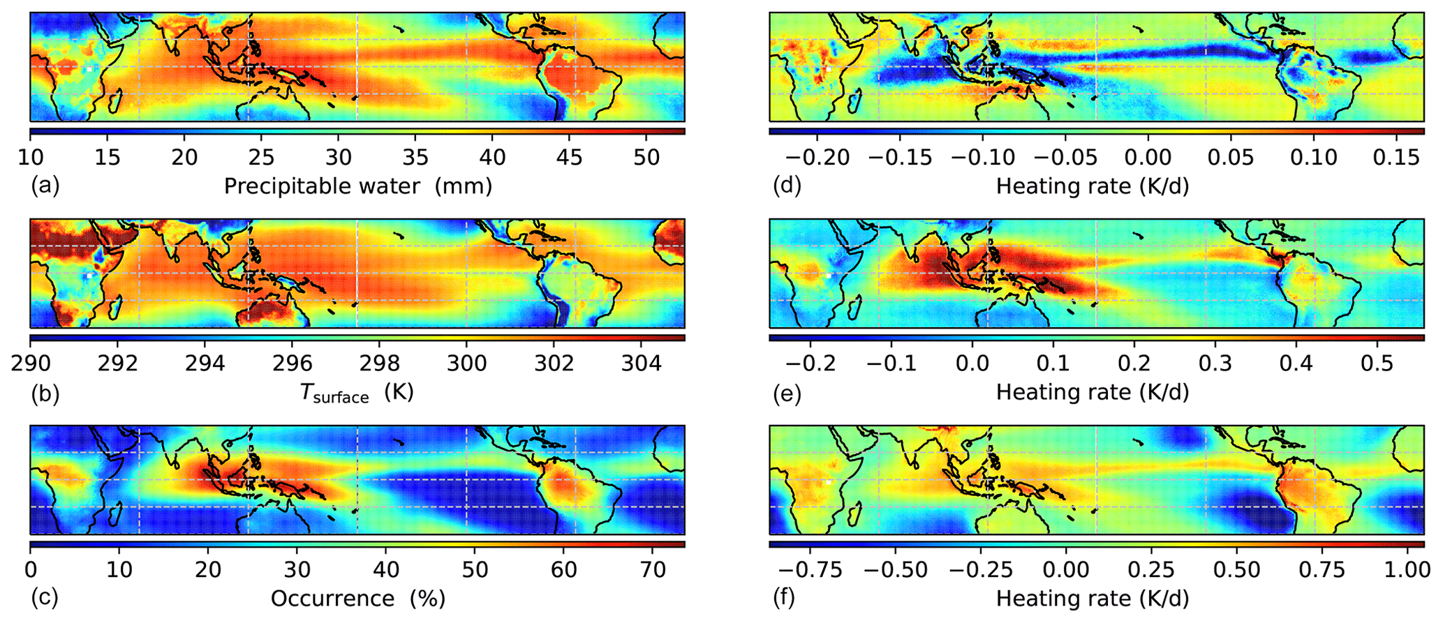
Figure 7Geographical maps of total precipitable water and surface temperature from ERA-Interim and frequency of occurrence of UT clouds from CIRS-AIRS (a, b, c) and of 24 h net cloud radiative heating effect in three atmospheric layers, integrated over 106 to 200 hPa, over 200 to 585 hPa and 585 to 900 hPa (d, e, f). Statistics of 16 years (2003–2018).
4.2 Relation between regional surface temperature and MCSs
A necessary condition for the onset of tropical deep convection, particularly over ocean, is a surface temperature (Tsurf) above a threshold of about 300 K (e.g. Gray, 1968; Graham and Barnett, 1987; Aumann et al., 2018), though other factors, such as available humidity (which may increase with low-level convergence), also affect the convective process. Though the shading of the thick anvils may cause some surface cooling during the day, slightly offset by the thinner cirrus (Wall et al., 2018), there should be more and deeper MCSs over warm regions than over cool regions. As in a changing climate the extension of warm regions may slightly increase, we compare in this section the properties of MCSs over warmer and over cooler regions.
Recently, Fueglistaler (2019) used the regions of the 30 % warmest sea surface temperature (SST) within the tropics as a proxy for regions of deep convective activity. Considering the distributions of the SST underneath the opaque part (cloud emissivity >0.9) of MCSs and underneath cold MCSs (near-cloud-top temperature TCb <210 K), they are indeed shifted towards warmer SST (Fig. S10). We derived the thresholds for the coolest 30 % and warmest 30 % tropical oceanic regions from ERA-Interim as 300 and 302 K, respectively. Therefore we use these two thresholds to compare the characteristics of MCSs in cool and in warm oceanic regions.
The tropics-wide 24 h mean net CRE of the MCSs depends on their frequency of occurrence, their height, horizontal extent and emissivity structure. First we study the effect of the relative occurrence frequency of the different cloud types (mid- and low-level clouds, UT clouds, thin cirrus, MCSs and thin cirrus associated with MCSs) on the effect of the total CRE. Figure 8 contrasts the CRE of the coolest 30 % and warmest 30 % ocean regions, for all clouds and when the specific cloud types are present. First of all, over warm regions, clouds, when present, have a heating effect over most of the troposphere, and this heating is mostly driven by MCSs. This is deduced from the strong similarity between the profiles of the present MCSs and those of all clouds. In addition, the UT thin cirrus heating linked to convection is slightly larger than the one of all thin cirrus, which indicates more and slightly thicker thin cirrus linked to convection than those produced in situ. Over cool regions low-level clouds also play an important role, with no heating between 200 and 600 hPa and a strong cooling around 820 hPa.
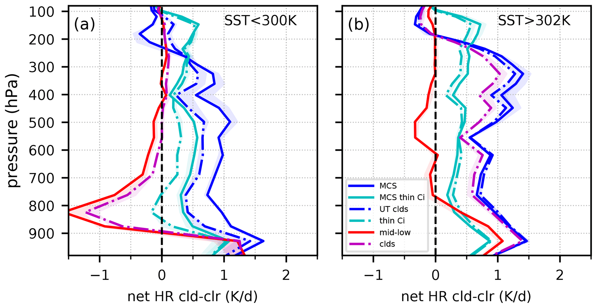
Figure 8Tropical 24 h mean cloud net radiative heating effect (magenta) within the troposphere above ocean, as well as the separate effects of low- and mid-level clouds (red), all UT clouds (dashed–dotted blue), thin cirrus (dashed–dotted cyan), MCSs (full blue line) and thin cirrus associated with MCSs (full cyan line), averaged over 15∘ N to 15∘ S, when the specific cloud types are present. (a) Regions with SST<300 K. (b) Regions with SST>302 K. These thresholds correspond to the 30 % coolest and warmest tropical oceanic regions.
The influence of emissivity structure is investigated by considering the 24 h mean net heating and cooling effects of the different parts of the MCSs, convective core, cirrus anvil and surrounding thin cirrus, when MCSs are present. These are presented in Fig. 9, for all tropical maritime MCSs and those over cool and warm ocean regions, respectively. As already seen in Fig. 3, the shape of the vertical profiles is quite different for the three parts of the MCSs. In the UT (at a height above 200 hPa), we observe an average cooling of about −2 K d−1 above the convective cores and a much reduced cooling above the cirrus anvil, while the thin cirrus heat the UT by about 0.5 K d−1. The troposphere below the height of 200 hPa is strongly heated by the convective cores, much less heated by the cirrus anvils and even less by the surrounding thin cirrus. However, as the convective cores only cover a small fraction of the systems (about 10 % on average), the average CRE of the MCSs corresponds to the one of the cirrus anvils. By contrasting cool and warm oceanic regions, the shape of the net radiative heating strengthens the hypothesis of MCSs with larger convective depth above the warm regions, with a cooling of the thicker parts of the MCSs shifted further up into the UT by 50 hPa, while the heating is extended over a broader vertical layer between 550 and 200 hPa. On the other hand, the thin cirrus net radiative heating of the UT of about 0.5 K d−1 is only associated with the deeper convective systems over the warm regions. These are mostly large MCSs with multiple convective cores.
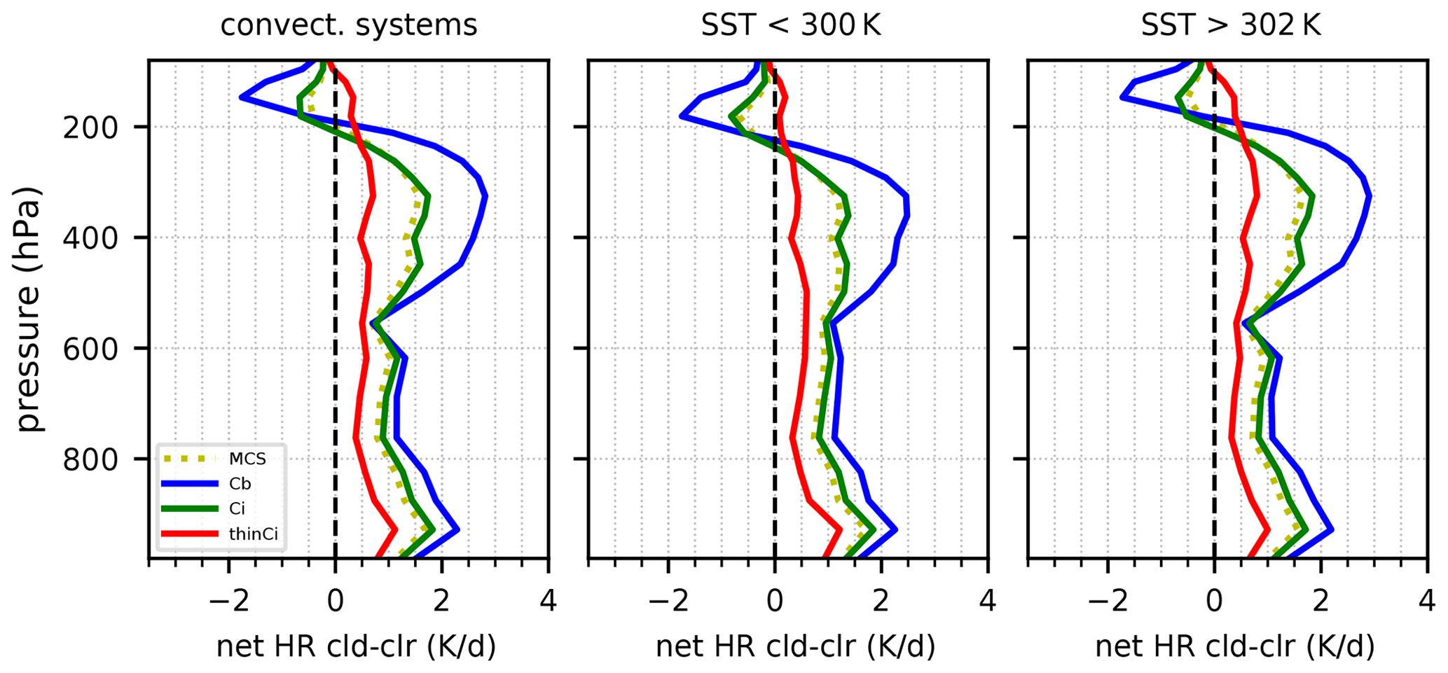
Figure 9Mean 24 h net radiative heating effect of tropical maritime MCSs, when present, and their convective cores (Cb), cirrus anvil (Ci) and surrounding thin cirrus (thinCi), separately for all MCSs (full line) and for those with single convective cores (dotted lines). Further distinguished are MCSs over the 30 % coolest areas (SST<300 K) and over the 30 % warmest areas (SST>302 K). Statistics of 15 years (2004–2018), averaged over 15∘ N to 15∘ S.
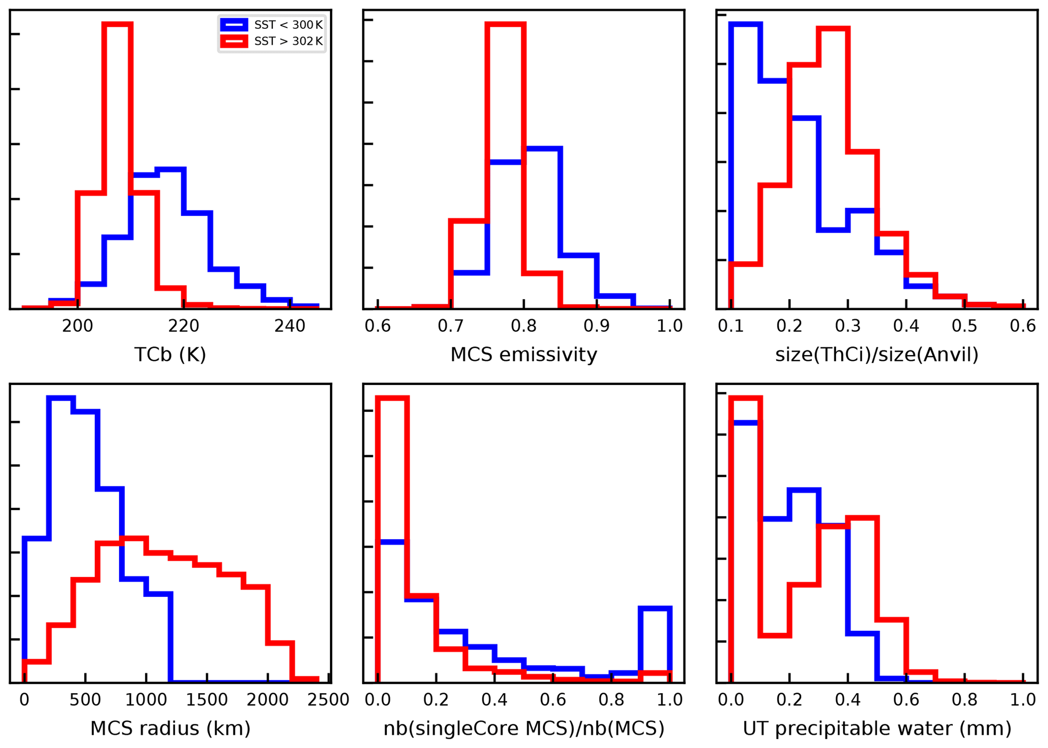
Figure 10Normalized distributions of maritime MCS properties: near-cloud-top temperature of convective cores, emissivity of convective cores and cirrus anvil, relative size of thin cirrus surrounding the anvil, radius of convective core and cirrus anvil, fraction of MCSs with single convective core and upper tropospheric precipitable water, separately for systems overlying cool and warm regions.
Figure 10 compares the properties of these maritime MCSs over cool and warm regions. In general, the warm regions are more humid according to the distributions of total precipitable water from ERA-Interim (not shown) and present also slightly more humidity in the upper troposphere (last panel of Fig. 10). The distributions in Fig. 10 indicate that maritime MCSs overlying warm regions have colder convective cores (given by their near-cloud-top temperature TCb), which means that they are extending higher into the troposphere and have also more often a larger horizontal extent (MCS radius of convective core and cirrus anvil), in agreement with a regional study by Horvath and Soden (2008). The area occupied by thin cirrus associated with MCSs, relative to the anvil area, is also larger. This can be explained by (i) a larger relative humidity at higher altitude and (ii) additional UT humidification originating from the convection (e.g. Luo et al., 2011). When convective systems are present over the cool regions, they seem to be more confined, consisting more often of systems with one single convective core (no.(singleCore MCS)/no.(MCS) close to 1), with a slightly larger average emissivity (MCS emissivity: averaged over convective cores and cirrus anvil). The latter is in agreement with a study of Del Genio et al. (2005), which revealed a decreasing detrainment and increasing precipitation efficiency within maritime MCSs when the underlying SST increases.
As mentioned at the beginning of this section, not only SST, but also other factors influence the properties of the MCSs. Therefore we also investigated the heating effects of the different parts of the MCSs over the tropical Atlantic, eastern Pacific, central Pacific and western Pacific (Fig. S11), with mean SST increasing from the Atlantic towards the western Pacific. Though differences in dynamics and atmospheric environment between these regions certainly also play a role (e.g. Henderson et al., 2018), the differences in the 24 h net radiative heating effect are larger between cool and warm periods within these regions than between these regions. From this, one may conclude that the slightly increasing CRE of the MCSs from the tropical Atlantic to the western Pacific on average can be mostly explained by increasing parts of warm SSTs from the tropical Atlantic towards the West Pacific.
4.3 Changes in tropical heating and in MCSs in dependence of tropical surface temperature anomaly
In Sect. 4.2 we have shown that the heating over the warmer tropical ocean regions is mostly influenced by MCSs and that the MCSs in these warmer regions also have a larger convective depth and are slightly larger, but with slightly smaller emissivity, than in the cooler regions. Using the available 15 years of HR fields and of MCS properties, we investigate in this section interannual variations in MCSs and in resulting atmospheric heating and cooling and try to relate these to tropical Tsurf anomalies and to phenomena which influence the interannual variability. Although the time period covered by AIRS observations may still not be long enough for climate change attribution, we note that the tropical Tsurf anomalies from ERA-Interim are very well correlated with global Tsurf anomalies (GISTEMP v4; Lenssen et al., 2019), with a Pearson correlation coefficient r of 0.91.
The mesoscale UT cloud systems cover 25.6 % of the tropical latitude band, with 80 % of their coverage from MCSs (having at least one convective core) and 6 % from thin cirrus systems. Moreover 48 % of the MCSs are cold MCSs with near-cloud-top temperature TCb <210 K. We estimate changes in the properties of the tropical MCSs in relation to tropical surface warming by determining linear regression slopes between the anomalies of the MCS properties and the tropical Tsurf anomalies, after smoothing the deseasonalized data by 12-month running means. This is a common method (e.g. Liu et al., 201; Stubenrauch et al., 2017), and uncertainties are derived from the residuals of the linear regression. Time series are presented in Figs. 11 to 13.
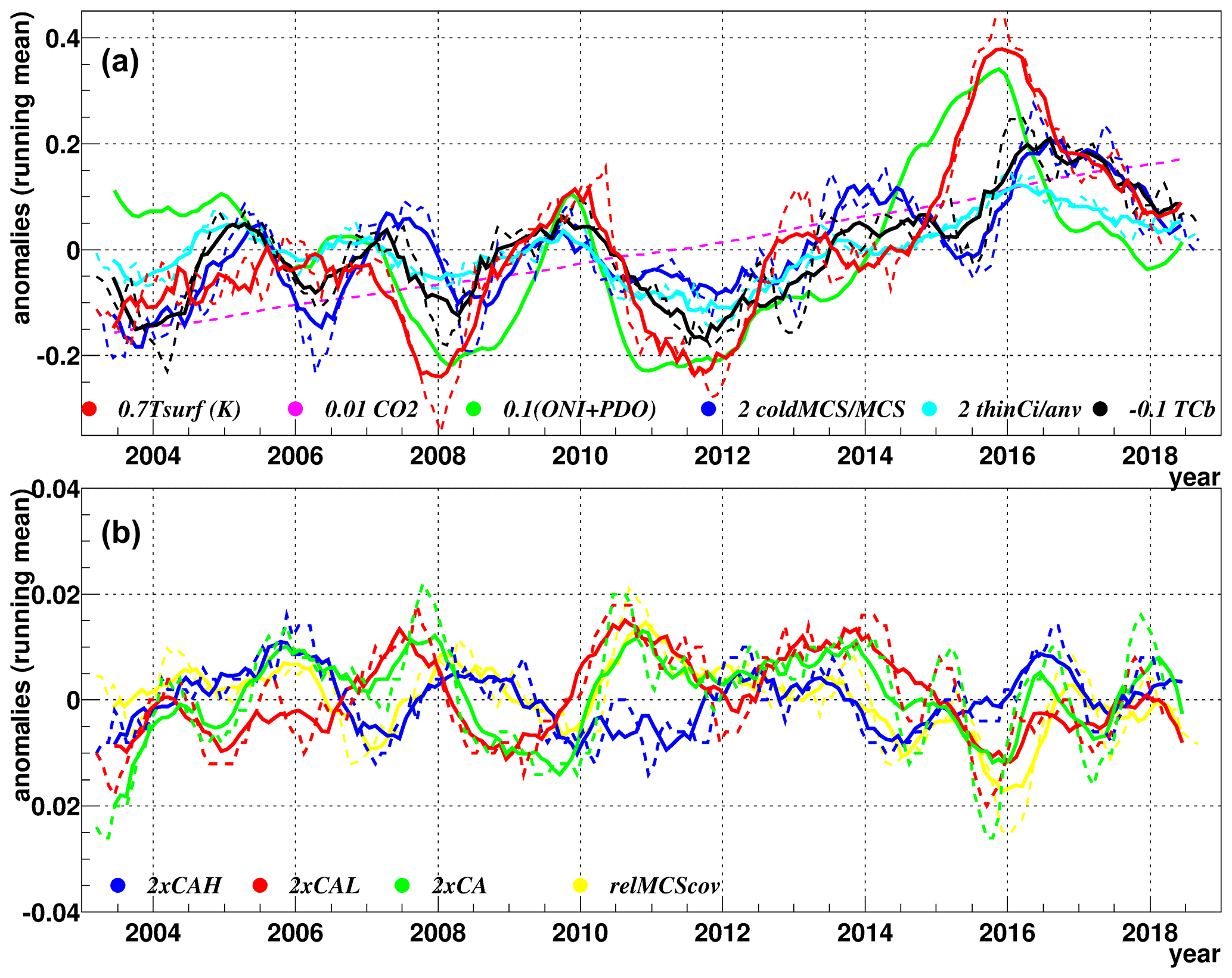
Figure 11(a) Time series of 12-month running means (bold lines) and 6-month running means of deseasonalized anomalies of tropical surface temperature (ERA-Interim), ENSO index (ONI) and Inter-decadal Pacific Oscillation (PDO) index, as well as coverage of cold MCSs over all MCSs (multiplied by 2), area of thin cirrus over area of total cirrus anvil (multiplied by 2), convective core temperature (in K, multiplied by −0.1) and increase of CO2 concentration (in ppm, multiplied by 0.01). (b) Time series of 12-month running means of deseasonalized anomalies of cloud cover (CA), UT cloud cover (CAH) and low-level cloud cover (CAL), multiplied by 2, and of relative MCS coverage.
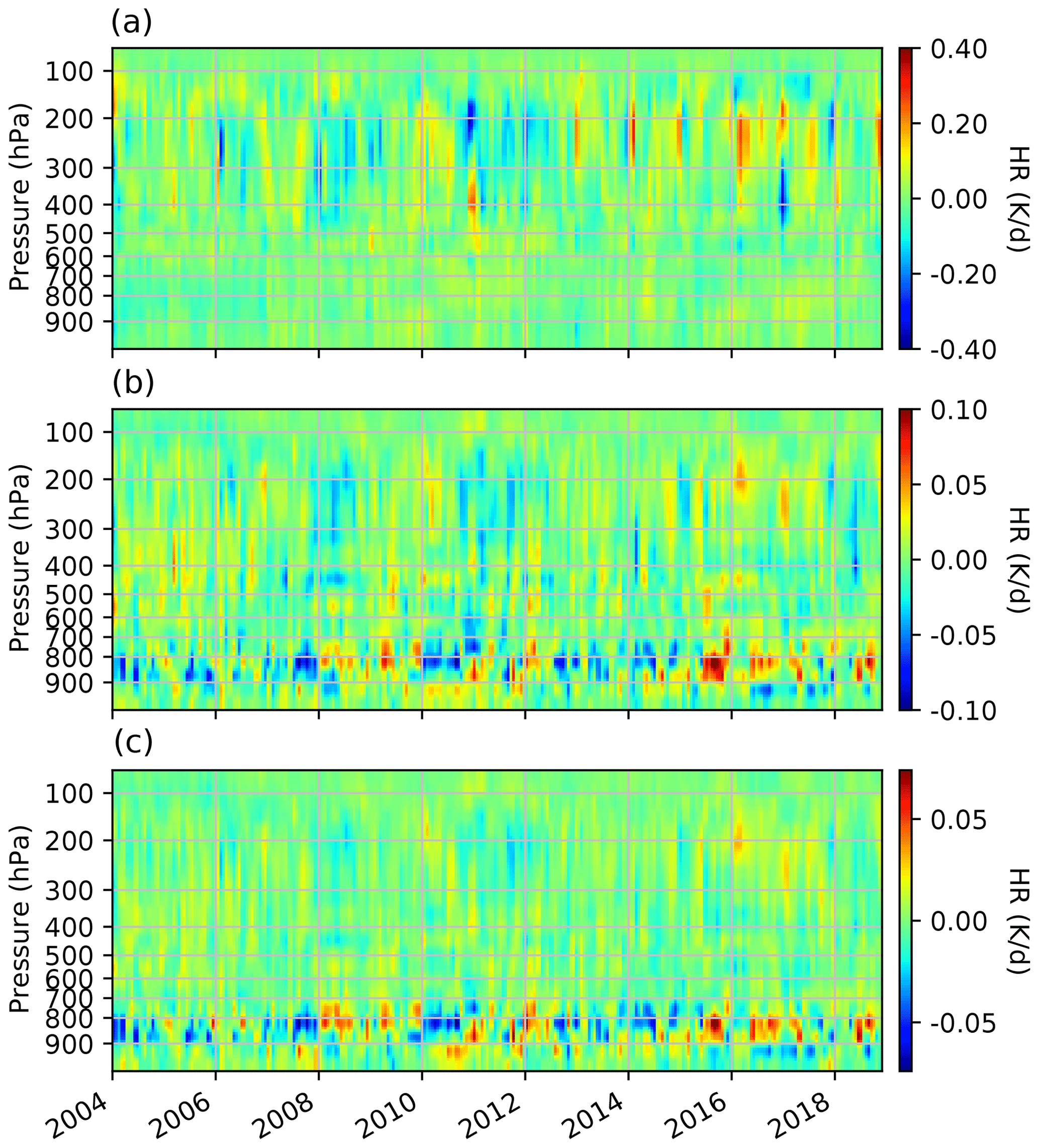
Figure 12Time series of deseasonalized anomalies of 24 h net cloud heating and cooling effects of MCSs (a) and of clouds (b), when present, and the CRE (c).
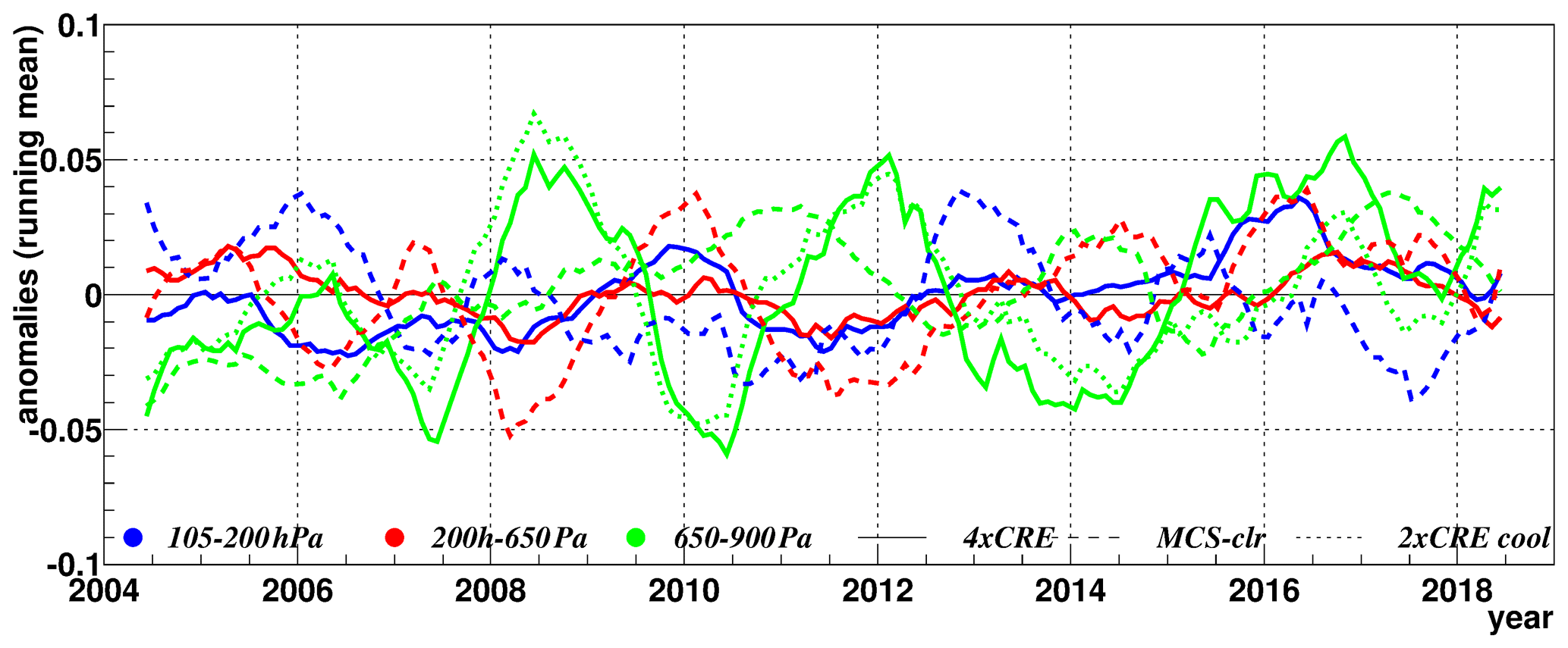
Figure 13Time series of 12-month running means of deseasonalized anomalies of 24 h net cloud heating and cooling effects of the CRE (full lines) and MCSs (broken lines), over three vertical layers, and of the CRE in the boundary layer (650–900 hPa) over cool regions (dotted green line).
The tropical Tsurf anomalies are related to the El Niño–Southern Oscillation (ENSO) and to the Interdecadal Pacific Oscillation (PDO), both with r=0.71, the PDO being influenced by ENSO (r=0.75). The Oceanic Niño Index (ONI) and the NCEI PDO index are provided by the National Oceanic and Atmospheric Administration (NOAA). El Niño (La Niña) events are linked to a positive (negative) tropical Tsurf anomaly. Their initiation is given by a local SST anomaly in the tropical Pacific, which then changes the east-west SST gradient, affecting the atmospheric circulation and the distribution of clouds. These phenomena have been extensively studied (e.g. Schumacher et al., 2004; Su and Jiang, 2013; Stephens et al., 2018b; Sullivan et al., 2019).
The coverage of all clouds, of low-level clouds, of UT clouds and of MCSs is stable over the whole period, with undulations of less than 0.01. While low-level and UT cloud cover show no significant correlations with anomalies of tropical Tsurf, ONI and PDO, total cloud cover and relative MCS cover show slight anti-correlations with ONI (r=0.62 and r=0.74, respectively), and the latter shows a very small decrease of % K−1 (r=0.7). On the other hand, we notice that MCSs get colder (deeper) with Tsurf warming (convective core near-top temperature decreasing by K K−1 with r=0.78), and thus the surrounding thin cirrus area relative to the anvil area slightly increases by % K−1, with r=0.85. When considering the coverage of cold MCSs relative to all MCSs, it increases by 13.2±1.3 % K−1, but this correlation is more uncertain (r=0.60). Yet, it is interesting to note that the coverage of cold MCSs seems to be lagged to the convective core temperature.
The CRE of MCSs is influenced by their depth as well as by their coverage. When comparing the oscillations of MCS coverage anomalies to those of cold MCS coverage anomalies, they seem to be slightly anti-correlated, so that there are phases when convective systems are deeper (colder), and the relative coverage of MCSs is reduced. This is in agreement with Zelinka and Hartmann (2010), who found during El Niño periods a decrease of high-level cloud amount as well as an increase in their height.
The time series of the anomalies of the 24 h net vertically resolved heating and cooling effects of MCSs shown in Fig. 12 reveal vertical dipole effects, which seem to be linked to ENSO variability and can be explained by changes in convective depth of the MCSs. The anomalies have values of about −0.4 and +0.4 K d−1, respectively. Figure 12 also presents the time series of the anomalies of the 24 h net vertically resolved heating and cooling effects of all clouds, when present, and of all clouds, weighted by their cover, all averaged over the latitude band 30∘ N to 30∘ S. The anomalies in the upper and middle troposphere have similar patterns as the ones for the MCSs, only much smaller in magnitude, because their relative frequency of occurrence is taken into account. We also observe strong cooling and heating anomaly patterns in the lower atmosphere, linked to the occurrence of stratocumulus and stratus cloud fields. There is evidence of a cooling in the atmospheric boundary layer (linked to low-level clouds) that is associated with warming in the upper and middle troposphere (linked to MCS activity), just balancing the opposite effects in warm and cool regions (see Fig. 8). In order to quantify the suggested correlations, we averaged these CRE anomalies over three atmospheric layers (100–200, 200–650 and 650–900 hPa) and analysed correlations between them and the variables displayed in Fig. 11. Figure 13 displays the time series of the CRE anomalies in these three layers for MCSs and for all clouds weighted by their coverage, as well as the latter in the 650–900 hPa layer over the cool regions (Tsurf<300 K). Considering MCSs, we observe the above-mentioned dipole effect between the 100–200 and the 200–650 hPa layers, with slightly more cooling near the tropopause when there is more heating in the atmosphere below, thus increasing the vertical gradients, during periods of warmer Tsurf (El Niño). Deeper MCSs correspond to a stronger heating in the 200–650 hPa layer (correlation with TCb: r=0.80). The correlations with Tsurf and ONI anomalies have values equal to 0.69 and 0.57, respectively, keeping in mind that ONI is an oceanic phenomenon, and we compare values to the HR anomalies of the whole tropics. When considering all clouds and all scenes, we find an interesting correlation between the CRE anomalies in the layer close to the tropopause and those of Tsurf (r=0.83 and r=0.86, respectively), suggesting a slight heating with warmer Tsurf, which is mostly due to more thin cirrus surrounding the anvils (r=0.70).
Finally, our hypothesis of an energetic connection between the convective regions and the subsidence regions can be consolidated by a correlation coefficient between the MCS heating in the 200–650 hPa layer (broken red line in Fig. 13) and the cooling in the 650–900 hPa layer of the cool regions (dotted green line in Fig. 13) with a value equal to 0.71. This confirms that within the tropics and subtropics the extent of the stratocumulus and stratus fields is energetically constrained by the height and extent of MCSs (e.g. Hang et al., 2019; Jakob et al., 2019). Based on these results it would be interesting to study in more detail possible lags in the time series at a finer timescale. A first study by Fueglistaler (2019) has shown transitions from an initial decrease in oceanic cloudiness due to lagged warming of the warmest waters to increased cloudiness in the decay phase of El Niño.
Radiative HR profiles can be derived using the active lidar and radar measurements from CALIPSO and CloudSat but only on narrow nadir tracks. On the other hand, AIRS, also part of the A-Train satellite constellation, provides cloud properties with a large instantaneous horizontal coverage. We constructed 3D HR fields within 30∘ N to 30∘ S, for the period 2003 to 2018, by using these radiative HRs for the training and applying the resulting ANN models on cloud properties from AIRS and atmospheric and surface properties from ECMWF meteorological reanalyses.
We demonstrated that non-linear ANN regression models, trained on large statistics of 4 years of collocated data, are appropriate methods to estimate tropical radiative HRs from about 40 cloud, atmospheric and surface properties. The column-integrated MAE is about 0.8 K d−1 (0.5 K d−1) for cloudy scenes and 0.4 K d−1 (0.3 K d−1) for clear sky in the LW (SW). Separate models for (i) Cb, (ii) cirrus and thin cirrus, (iii) mid- and low-level clouds and (iv) clear sky, independently over ocean and over land, perform slightly better, with mean predicted radiative HRs very close to the “observed” ones, with uncertainties within 0.25 K d−1 per layer. The improvement is most noticeable for Cb, with uncertainties around the maxima of LW cooling and SW heating due to small vertical shifts in the HR profiles. The monthly mean horizontal structures of the predicted HR fields agree well with the original ones from CALIPSO–CloudSat, but they appear more clearly, due to the lateral expansion.
We have produced the longest tropical HR dataset available by applying the ANN models to 15 years of combined AIRS and ECMWF data. By studying the long-term temporal behaviour of the HRs, in particular in relation to tropical Tsurf variability, we have demonstrated that the regression models produce also reliable results outside the training period (assuming a non-changing relationship between the input parameters and the HRs).
We confirm that most of the total cloud net radiative heating effect in the deep tropics (15∘ N–15∘ S) comes from UT clouds. These clouds have a 24 h mean net radiative heating effect of about 0.3 K d−1 from 250 hPa downward, enhancing the column-integrated latent heating by 22±3 %. This value is only slightly larger than earlier results of about 20 % (Li et al., 2013), using ISCCP cloud data, but our result may still be slightly underestimated because of the cloud contamination of the clear-sky scenes identified by AIRS and the slightly underestimated LW warming above 12 km in the original FLXHR-LIDAR (R04) data linked to cirrus microphysical assumptions. Yet, the shape of the heating profiles compared to those of Li et al. (2013) is significantly different, with our estimation indicating a much more vertically extended heating. This suggests an underestimation of the heating in the middle troposphere of the earlier result, which can be explained by the shading effect of underlying low-level clouds on ground-based measurements and by a mixture of cirrus and surrounding single-layer low-level clouds linked to a coarse spatial resolution of the cloud regime approach.
In general, the UT cloud effect is a strong heating of the UT during daytime and a strong lower tropospheric heating during nighttime, leading to opposite diurnal vertical gradients. The heating profile shapes of the convective cores, cirrus anvil and surrounding thin cirrus of MCSs differ significantly: the troposphere from 200 hPa downward is strongly heated by the convective cores, less heated by the cirrus anvils and even less by the surrounding thin cirrus. However, as the convective cores only cover a small fraction of the systems, the average heating effect of the MCSs corresponds to the one of the cirrus anvils.
Over the warmest 30 % ocean regions, the heating is mostly driven by MCSs, which also have a larger convective depth than the ones over the coolest 30 % ocean regions. The consequence is a heating over a broader vertical layer, between 550 and 200 hPa. The thin cirrus linked to the MCSs in these regions heat the UT by about 0.5 K d−1, more than the in situ formed cirrus. The latter play a more important role over cool regions, as well as mid- and low-level clouds (over ocean), with much less heating between 200 and 900 hPa.
During the time period 2003 to 2018, the coverage of all clouds, UT clouds, low clouds and MCSs is relatively stable, with undulations less than 1 %. On the other hand, MCSs get colder (deeper) with tropical Tsurf warming (by K K−1), and thus the surrounding thin cirrus area relative to the anvil area slightly increases by % K−1.
The time series of the anomalies of the 24 h net vertical heating and cooling effects of clouds and in particular of the MCSs exhibits vertical dipole effects, related to tropical Tsurf variability and explained by changes in convective depth of the MCSs: during periods of warmer tropical Tsurf (El Niño), the HR vertical structure anomaly suggests deeper MCSs, with vertically broader heating. The data also reveal a small heating effect in the layer close the tropopause with tropical surface warming, mostly due to more thin cirrus surrounding the anvils of the MCSs. Finally, we highlighted a correlation of the MCS heating in the upper and middle troposphere and the (low-level) cloud cooling in the lower atmosphere in the cool regions (r=0.72). This shows, in agreement with other studies, that within the tropics and subtropics the extent of the low-level cloud fields is energetically constrained by the height and extent of the MCSs. Lags between the different variables in the time series will be further explored at a finer timescale.
The new database of the radiative heating rate fields builds the basis for future studies. Therefore, we will add the latent heating profiles derived from the Tropical Rainfall Measuring Mission (TRMM) to this synergistic dataset, which provides for the first time a 3D view of the radiative heating profiles over a long time period. As the coincidences in time with AIRS are small, again we will use machine learning techniques, similar to the ones described in this article. This database of UT cloud systems is being constructed within the framework of the GEWEX (Global Energy and Water Exchanges) Process Evaluation Study on Upper Tropospheric Clouds and Convection (GEWEX UTCC PROES; https://gewex-utcc-proes.aeris-data.fr/, last access: January 2020) to advance our knowledge on the climate feedbacks of UT clouds. In general, climate feedback studies are undertaken by climate model simulations, which rely upon their representation of convection and detrainment. The cloud system approach has already proved its usefulness in the evaluation of a new bulk ice cloud scheme in the LMD general circulation model (GCM; Stubenrauch et al., 2019), and the HRs may be used to distinguish between parameterizations of ice cloud radiative properties. Furthermore, this database, in particular when including the total 3D diabatic heating, will be used to quantify the dynamical response of the climate system to the atmospheric heating induced by the anvil cirrus, refining and extending the studies of Schumacher et al. (2004) and Li et al. (2013).
In the future we will train the ANN models again with the improved version of the FLXHR-LIDAR data and a new version of the CIRS data (using ERA5 ancillary data, as ERA-Interim data production ceased in August 2019).
CIRS data have been produced by the French Data Centre AERIS and are distributed at https://cirs.aeris-data.fr/ (last access: 15 January 2021, CIRS, 2021). Monthly indices of ENSO strength (ONI) and of PDO were obtained from NOAA (https://origin.cpc.ncep.noaa.gov/products/analysis_monitoring/ensostuff/detrend.nino34.ascii.txt, last access: February 2020, NOAA-ONI, 2020, and https://www.ncdc.noaa.gov/teleconnections/pdo/, last access: February 2020, NOAA-PDO, 2020, respectively), both derived from Extended Reconstructed Sea Surface Temperature (ERSSTv5).
The supplement related to this article is available online at: https://doi.org/10.5194/acp-21-1015-2021-supplement.
SEP and FH contributed to Sect. 3 by developing the ANN model code, preparing the data and initializing the evaluation. GC contributed to the analyses in Sect. 4. They also contributed to improvements of the manuscript. CJS developed the concept, improved the ANN method, produced and analysed the long-term dataset, and wrote the manuscript.
The authors declare that they have no conflict of interest.
This work is supported by the Centre National de la Recherche Scientifique (CNRS) and the Centre National d'Etudes Spatiales (CNES). The authors thank the members of the AIRS, CALIPSO and CloudSat science teams for their efforts and cooperation in providing the data, as well as the engineers and space agencies who control the data quality. The authors also want to thank Anton Kaifel and Andrew Snauffer for inspiring discussions as well as two reviewers for their thoughtful comments which improved the quality of the paper.
This paper was edited by Manish Shrivastava and reviewed by two anonymous referees.
Ackerman, T. P., Liou, K.-N., Valero, F. P. J., and Pfister, L.: Heating Rates in Tropical Anvils, J. Atmos. Sci., 45, 1606–1623, https://doi.org/10.1175/1520-0469(1988)045<1606:HRITA>2.0.CO;2, 1988.
Aumann, H. H., Behrangi, A., and Wang, Y.: Increased Frequency of Extreme Tropical Deep Convection: AIRS Observations and Climate Model Predictions, Geophys. Res. Lett., 45, 13530–13537, https://doi.org/10.1029/2018GL079423, 2018.
Austin, R. T., Heymsfield, A. J., and Stephens, G. L.: Retrieval of ice cloud microphysical parameters using the CloudSat millimeter-wave radar and temperature, J. Geophys. Res., 114, D00A23, https://doi.org/10.1029/2008JD010049, 2009.
Bergman, J. W. and Hendon, H. H.: Cloud Radiative Forcing of the Low-Latitude Tropospheric Circulation: Linear Calculations, J. Atmos. Sci., 57, 2225–2245, https://doi.org/10.1175/1520-0469(2000)057<2225:CRFOTL>2.0.CO;2, 2000.
Boucher, O., Randall, D., Artaxo, P., Bretherton, C., Feingold, G., Forster, P., Kerminen, V.-M., Kondo, Y., Liao, H., Lohmann, U., Rasch, P., Satheesh, S.K., Sherwood, S., Stevens, B., and Zhang, X. Y.: Clouds and aerosols, in: Climate Change 2013: The Physical Science Basis. Contribution of Working Group I to the Fifth Assessment Report of the Intergovernmental Panel on Climate Change, edited by: Stocker, T. F., Qin, D., Plattner, G.-K., Tignor, M., Allen, S. K., Doschung, J., Nauels, A., Xia, Y., Bex, V., and Midgley, P. M., Cambridge University Press, Cambridge, UK, 571–657, https://doi.org/10.1017/CBO9781107415324.01, 2013.
Chahine, M. T., Pagano, T. S., Aumann, H. H., Atlas, R., Barnet, C., Blaisdell, J., Chen, L., Divakarla, M., Fetzer, E. J., Goldberg, M., Gautier, C., Granger, S., Hannon, S., Irion, F. W., Kakar, R., Kalnay, E., Lambrigtsen, B. H., Lee, S., Le Marshall, J., McMillan, W. W., McMillin, L., Olsen, E. T., Revercomb, H., Rosenkranz, P., Smith, W. L., Staelin, D., Strow, L. L., Susskind, J., Tobin, D., Wolf, W., and Zhou, L.: AIRS: Improving weather forecasting and providing new data on greenhouse gases, B. A. Meteorol. Soc., 87, 911–926, https://doi.org/10.1175/BAMS-87-7-911, 2006.
Chédin, A., Serrar, S., Scott, N. A., Crevoisier, C., and Armante, R.: First global measurement of midtropospheric CO2 from NOAA polar satellites: Tropical zone, J. Geophys. Res., 108, 4581, https://doi.org/10.1029/2003JD003439, 2003.
CIRS (Clouds from IR Sounders): https://cirs.aeris-data.fr/, last access: 15 January 2021.
Dee, D. P., Uppala, S. M., Simmons, A. J., Berrisford, P., Poli, P., Kobayashi, S., Andrae, U., Balmaseda, M. A., Balsamo, G., Bauer, P., Bechtold, P., Beljaars, A. C. M., van de Berg, L., Bidlot, J., Bormann, N., Delsol, C., Dragani, R., Fuentes, M., Geer, A. J., Haimberger, L., Healy, S. B., Hersbach, H., Holm, E. V., Isaksen, L., Kallberg, P., Kohler, M., Matricardi, M., McNally, A. P., Monge-Sanz, B. M., Morcrette, J.-J., Park, B.-K., Peubey, C., de Rosnay, P., Tavolato, C., Thepaut, J.-N., and Vitart, F.: The ERA-Interim reanalysis: configuration and performance of the data assimilation system, Q. J. Roy. Meteor. Soc., 137, 553–597, https://doi.org/10.1002/qj.828, 2011.
Del Genio, A. D., Kovari, W., Yao, M.-S., and Jonas, J.: Cumulus microphysics and climate sensitivity, J. Climate, 18, 2376–2387, https://doi.org/10.1175/JCLI3413.1, 2005.
Deng, M., Mace, G. G., Wang, Z., and Lawson, R. P.: Evaluation of Several A-Train Ice Cloud Retrieval Products with In Situ Measurements Collected during the SPARTICUS Campaign, J. Appl. Meteor. Climatol., 52, 1014–1030, https://doi.org/10.1175/JAMC-D-12-054.1, 2013.
Feofilov, A. G. and Stubenrauch, C. J.: Diurnal variation of high-level clouds from the synergy of AIRS and IASI space-borne infrared sounders, Atmos. Chem. Phys., 19, 13957–13972, https://doi.org/10.5194/acp-19-13957-2019, 2019.
Feofilov, A. G., Stubenrauch, C. J., and Delanoë, J.: Ice water content vertical profiles of high-level clouds: classification and impact on radiative fluxes, Atmos. Chem. Phys., 15, 12327–12344, https://doi.org/10.5194/acp-15-12327-2015, 2015.
Fueglistaler, S.: Observational Evidence for Two Modes of Coupling Between Sea Surface Temperatures, Tropospheric Temperature Profile, and Shortwave Cloud Radiative Effect in the Tropics, Geophys. Res. Lett., 46, 9890–9898, https://doi.org/10.1029/2019GL083990, 2019.
Graham, N. E. and Barnett, T. P.: Sea Surface Temperature, Surface Wind Divergence, and Convection over Tropical Oceans, Science, 238, 657–659, https//doi.org/10.1126/science.238.4827.657, 1987.
Gray, W.: A global view of the origin of tropical disturbances and storms, Mon. Weather Rev., 96, 669–700, https://doi.org/10.1175/1520-0493(1968)096<0669:GVOTOO>2.0.CO;2, 1968.
Guignard, A., Stubenrauch, C. J., Baran, A. J., and Armante, R.: Bulk microphysical properties of semi-transparent cirrus from AIRS: a six year global climatology and statistical analysis in synergy with geometrical profiling data from CloudSat-CALIPSO, Atmos. Chem. Phys., 12, 503–525, https://doi.org/10.5194/acp-12-503-2012, 2012.
Ham, S.-H., Kato, S., Rose, F. G., Winker, D., L'Ecuyer, T., Mace, G. G., Painemal, D., Sun-Mack, S., Chen, Y., and Miller, W. F.: Cloud occurrences and cloudradiative effects (CREs) fromCERES-CALIPSO-CloudSat-MODIS (CCCM) and CloudSat radar-lidar (RL) products, J. Geophys. Res.-Atmos., 122, 8852–8884, https://doi.org/10.1002/2017JD026725, 2017.
Hang, Y., L'Ecuyer, T. S., Henderson, D. S., Matus, A. V., and Wang, Z.: Reassessing the Effect of Cloud Type on Earth's Energy Balance in the Age of Active Spaceborne Observations. Part II: Atmospheric Heating, J. Climate, 32, 6219–6236, https://doi.org/10.1175/JCLI-D-18-0754.1, 2019.
Haynes, J. M., L'Ecuyer, T., Stephens, G. L., Miller, S. D., Mitrescu, C., Wood, N. B., and Tanelli, S.: Rainfall retrieval over the ocean with spacenorne W-band radar, J. Geophys. Res.-Atmos., 114, D00A22, https://doi.org/10.1029/2008JD009973, 2009.
Henderson, D. S., L'Ecuyer, T., Stephens, G. L, Partain, P., and Sekiguchi, M.: A Multisensor Perspective on the Radiative Impacts of Clouds and Aerosols, J. Appl. Meteor. Climatol., 52, 853–871, https://doi.org/10.1175/JAMC-D-12-025.1, 2013.
Henderson, D. S., Kummerow, C. D., and Berg, W.: ENSO Influence on TRMM Tropical Oceanic Precipitation Characteristics and Rain Rates, J. Climate, 31, 3979–3989, https://doi.org/10.1175/JCLI-D-17-0276.1, 2018.
Hersbach, H., Bell, B., Berrisford, P., Hirahara, S., Horányi, A., Muñoz-Sabater, J., Nicolas, J., Peubey, C., Radu, R., Schepers, D., Simmons, A., Soci, C., Abdalla, S., Abellan, X., Balsamo, G., Bechtold, P., Biavati, G., Bidlot, J., Bonavita, M., De Chiara, G., Dahlgren, P., Dee, D., Diamantakis, M., Dragani, R., Flemming, J., Forbes, R., Fuentes, M., Geer, A., Haimberger, L., Healy, S., Hogan, R. J., Hólm, E. Janisková, M., Keeley, S., Laloyaux, P., Lopez, P., Lupu, C., Radnoti, G., de Rosnay, P., Rozum, I., Vamborg, F., Villaume, S., and Thépaut, J.-N.: The ERA5 global reanalysis, Q. J. Roy. Meteor. Soc., 146, 1999–2049, https://doi.org/10.1002/qj.3803, 2020.
Horvath, A. and Soden, B. J.: Lagrangian diagnostics of tropical deep convection and its effect upon upper-tropospheric humidity, J. Climate, 21, 1013–1028, https://doi.org/10.1175/2007JCLI1786.1, 2008.
Houze Jr., R. A.: Mesoscale convective systems, Rev. Geophys., 42, RG4003, https://doi.org/10.1029/2004RG000150, 2004.
Igel, M. R., Drager, A. J., and Van Den Heever, S. C.: A CloudSat cloud object partitioning technique and assessment and integration of deep convective anvil sensitivities to sea surface temperature, J. Geophys. Res., 119, 10515–10535, https://doi.org/10.1002/2014JD021717, 2014.
Jakob, C., Singh, M. S., and Jungandreas, L.: Radiative convective equilibrium and organized convection: An observational perspective, J. Geophys. Res.-Atmos., 124, 5418–5430, https://doi.org/10.1029/2018JD030092, 2019.
Kingma, D. P. and Ba, J.: Adam: A Method for Stochastic Optimization, 3rd Int. Conf. for Learning Representations, San, Diego, 2015, arXiv [preprint], arXiv:1412.6980v9, 30 January 2017.
Kleynhans, T., Montanaro, M., Gerace, A., and Kanan, C.: Predicting Top-of-Atmosphere Thermal Radiance Using MERRA-2 Atmospheric Data with Deep Learning, Remote Sens., 9, 1133, https://doi.org/10.3390/rs9111133, 2017.
L'Ecuyer, T. S., Wood, N. B., Haladay, T., Stephens, G. L., and Stackhouse Jr., P. W.: Impact of clouds on atmospheric heating based on the R04 CloudSat fluxes and heating rates data set, J. Geophys. Res., 113, D00A15, https://doi.org/10.1029/2008JD009951, 2008.
L'Ecuyer, T. and McGarragh, G.: A 10-Year Climatology of Tropical Radiative Heating and Its Vertical Structure from TRMM Observations, J. Climate, 23, 519–541, https://doi.org/10.1175/2009JCLI3018.1, 2010.
Lenssen, N., Schmidt, G., Hansen, J., Menne, M., Persin, A., Ruedy, R., and Zyss, D., Improvements in the GISTEMP uncertainty model, J. Geophys. Res.-Atmos., 124, 6307–6326, https://doi.org/10.1029/2018JD029522, 2019.
Levy, R., Remer, L., Tanré, D., Mattoo, S., and Kaufman, Y.: Algorithm for remote sensing of tropospheric aerosol over dark targets from MODIS: Collections 005 and 051: Revision 2, MODIS Algorithm Theoretical Basis Document, NASA GSFC, Maryland, USA, 87 pp., available at: https://modis-images.gsfc.nasa.gov/_docs/MOD04-MYD04_ATBD_C005.pdf (last access: January 2021), 2009.
Li, W., Schumacher, C., and McFarlane, S. A.: Radiative heating of the ISCCP upper level cloud regimes and its impact on the large-scale tropical circulation, J. Geophys. Res.-Atmos., 118, 592–604, https://doi.org/10.1002/jgrd.50114, 2013.
Liu, R., Liou, K.-N., Su, H., Gu, Y., Zhao, B., Jiang, J. H., and Liu, S. C.: High cloud variations with surface temperature from 2002 to 2015: Contributions to atmospheric radiative cooling rate and precipitation changes, J. Geophys. Res.-Atmos., 122, 5457–5471, https://doi.org/10.1002/2016JD026303, 2017.
Luo, Z., Kley, D., Johnson, R. H., Liu, G. Y., Nawrath, S., and Smit, H. G. J.: Influence of Sea Surface Temperature on Humidity and Temperature in the Outflow of Tropical Deep Convection, J. Climate, 25, 1340–1348, https://doi.org/10.1175/2011JCLI4124.1, 2011.
Mace, G. G., Zhang, Q., Vaughan, M., Marchand, R., Stephens, G., Trepte, C., and Winker, D.: A description of hydrometeor layer occurrence statistics derived from the first year of merged Cloudsat and CALIPSO data, J. Geophys. Res., 114, D00A26, https://doi.org/10.1029/2007JD009755, 2009.
Mather, J. H., McFarlane, S. A., Miller, M. A., and Johnson, K. L.: Cloud products and associated heating rates in the Tropical Western Pacific, J. Geophys. Res., 112, D05201, https://doi.org/10.1029/2006JD007555, 2007.
Matus, A. and L'Ecuyer, T. S.: The role of cloud phase in Earth's radiation budget, J. Geophys. Res.-Atmos., 122, 2559–2578, https://doi.org/10.1002/2016JD025951, 2017.
NOAA-ONI: https://origin.cpc.ncep.noaa.gov/products/analysis_monitoring/ensostuff/detrend.nino34.ascii.txt, last access: February 2020.
NOAA-PDO: https://www.ncdc.noaa.gov/teleconnections/pdo/, last access: February 2020.
Oreopoulos, L., Cho, N., Lee, D., and Kato, S.: Radiative effects of global MODIS cloud regimes, J. Geophys. Res.-Atmos., 121, 2299–2317, https://doi.org/10.1002/2015JD024502, 2016.
Paul, M., Aires, F., Prigent, C., Trigo, I., and Bernardo, F.: An innovative physical scheme to retrieve simultaneously surface temperature and emissivities using high spectral infrared observations from IASI, J. Geophys. Res., 117, D11302, https://doi.org/10.1029/2011JD017296, 2012.
Protat, A., Young, S. A., McFarlane, S. A., L'Ecuyer, T., Mace, G. G., Comstock, J. M., Long, C. N., Berry, E., and Delanoë, J.: Reconciling Ground-Based and Space-Based Estimates of the Frequency of Occurrence and Radiative Effect of Clouds around Darwin, Australia, J. Appl. Meteor. Climatol., 53, 456–478, https://doi.org/10.1175/JAMC-D-13-072.1, 2014.
Protopapadaki, S. E., Stubenrauch, C. J., and Feofilov, A. G.: Upper tropospheric cloud systems derived from IR sounders: properties of cirrus anvils in the tropics, Atmos. Chem. Phys., 17, 3845–3859, https://doi.org/10.5194/acp-17-3845-2017, 2017.
Ritter, B. and Geleyn, J.-F.: A comprehensive radiation scheme for numerical weather prediction models with potential applications in climate simulations, Mon. Weather Rev., 120, 303–325, https://doi.org/10.1175/1520-0493(1992)120<0303:ACRSFN>2.0.CO;2, 1992.
Roca, R., Aublanc, J., Chambon, P., Fiolleau, T., and Viltard, N.: Robust Observational Quantification of the Contribution of Mesoscale Convective Systems to Rainfall in the Tropics, J. Climate, 27, 4952–4958, https://doi.org/10.1175/JCLI-D-13-00628.1, 2014.
Rossow, W. B., Tselioudis, G., Polak, A., and Jakob, C.: Tropical climate described as a distribution of weather states indicated by distinct mesoscale cloud property mixtures, Geophys. Res. Lett., 32, L21812, https://doi.org/10.1029/2005GL024584, 2005.
Schumacher, C., Houze, R. A., and Kraucunas, I.: The Tropical Dynamical Response to Latent Heating Estimates Derived from the TRMM Precipitation Radar, J. Atmos. Sci., 61, 1341–1358, https://doi.org/10.1175/1520-0469(2004)061<1341:TTDRTL>2.0.CO;2, 2004.
Sherwood, S. C., Ramanathan, V., Barnett, T., Tyree, M., and Roeckner, E.: Response of an atmospheric GCM to radiative forcing of tropical clouds, J. Geophys. Res., 99, 20829–20845, https://doi.org/10.1002/qj.49711448209, 1994.
Slingo, J. M. and Slingo, A.: The response of a general circulation model to cloud longwave radiative forcing. II: Further studies, Q. J. Roy. Meteor. Soc., 117, 333–364, https://doi.org/10.1002/qj.49711448209, 1991.
Snauffer, A. M., Hsieh, W. W., Cannon, A. J., and Schnorbus, M. A.: Improving gridded snow water equivalent products in British Columbia, Canada: multi-source data fusion by neural network models, The Cryosphere, 12, 891–905, https://doi.org/10.5194/tc-12-891-2018, 2018.
Sohn, B.-J.: Cloud-Induced Infrared Radiative Heating and Its Implications for Large-Scale Tropical Circulations, J. Atmos. Sci., 56, 2657–2672, https://doi.org/10.1175/1520-0469(1999)056<2657:CIIRHA>2.0.CO;2, 1999.
Stein, T. H. M., Holloway, C. E., Tobin, I., and Bony, S.: Observed relationships between cloud vertical structure and convective aggregation over tropical ocean, J. Climate, 30, 2187–2207, https://doi.org/10.1175/JCLI-D-16-0125.1, 2017.
Stephens, G. L. and Webster, P. J.: Cloud decoupling of surface and planetary radiative budgets, J. Atmos. Sci., 41, 681–686, https://doi.org/10.1175/1520-0469(1984)041<0681:CDOTSA>2.0.CO;2, 1984.
Stephens, G. L., Webster, P. J., Johnson, R. H., Engelen, R., and L'Ecuyer, T.: Observational Evidence for the Mutual Regulation of the Tropical Hydrological Cycle and Tropical Sea Surface Temperatures, J. Climate, 17, 2213–2224, https://doi.org/10.1175/1520-0442(2004)017<2213:OEFTMR>2.0.CO;2, 2004.
Stephens, G. L, Van den Heever, S., and Pakula, L. A.: Radiative Convective Feedback in Idealized States of Radiative-Convective Equilibrium, J. Atmos. Sci., 65, 3899–3916, https://doi.org/10.1175/2008JAS2524.1, 2008.
Stephens, G. L., Winker, D., Pelon, J., Trepte, C., Vane, D. G., Yuhas, C., L'Ecuyer, T., and Lebsock, M.: CloudSat and CALIPSO within the A-Train: Ten Years of Actively Observing the Earth System, B. Am. Meteor. Soc., 83, 1771–1790, https://doi.org/10.1175/BAMS-D-16-0324.1, 2018a.
Stephens, G. L., Hakuba, M. Z., Webb, M., Lebsock, M., Yue, Q., Kahn, B. H., Hristova-Veleva, S., Rapp, A., Stubenrauch, C., Elsaesser, G. S., and Slingo, J.: Regional intensification of the tropical hydrological cycle during ENSO, Geophys. Res. Lett., 45, 4361–4370, https://doi.org/10.1029/2018GL077598, 2018b.
Strahler, A. H., Muller, J.-P., and MODIS Science Team Members: MODIS BRDF/Albedo Product: Algorithm Theoretical Basis Document Version 5.0, MODIS Product ID: ATBD-MOD-43, NASA GSFC, Maryland, USA, available at: https://modis.gsfc.nasa.gov/data/atbd/atbd_mod09.pdf (last access January 2021), 1999.
Stubenrauch, C. J., Chédin, A., Armante, R., and Scott, N. A.: Clouds as Seen by Satellite Sounders (3I) and Imagers (ISCCP): II) A New Approach for Cloud Parameter Determination in the 3I Algorithms, J. Climate, 12, 2214–2223, https://doi.org/10.1175/1520-0442(1999)012<2214:CASBSS>2.0.CO;2, 1999.
Stubenrauch, C. J. and Schumann, U.: Impact of air traffic on cirrus coverage, Geophys. Res. Lett., 32, L14813, https://doi.org/10.1029/2005GL022707, 2005.
Stubenrauch, C. J., Cros, S., Guignard, A., and Lamquin, N.: A 6-year global cloud climatology from the Atmospheric InfraRed Sounder AIRS and a statistical analysis in synergy with CALIPSO and CloudSat, Atmos. Chem. Phys., 10, 7197–7214, https://doi.org/10.5194/acp-10-7197-2010, 2010.
Stubenrauch, C. J.,Rossow, W. B. ,and Kinne, S.: Assessment of global cloud datasets from satellites: A project of the World Climate Research Programme Global Energy and Water Cycle Experiment (GEWEX) Radiation Panel, WCRP Rep. 23/2012, 176 pp., available at: https://www.wcrp-climate.org/documents/GEWEX_Cloud_Assessment_2012.pdf, last access: January 2020), 2012.
Stubenrauch, C. J., Rossow, W. B., Kinne, S., Ackerman, S., Cesana, G., Chepfer, H., Di Girolamo, L., Getzewich, B., Guignard, A., Heidinger, A., Maddux, B., Menzel, P., Minnis, P., Pearl, C., Platnick, S., Poulsen, C., Riedi, J., Sun-Mack, S., Walther, A., Winker, D., Zeng, S., and Zhao, G.: Assessment of Global Cloud Datasets from Satellites: Project and Database initiated by the GEWEX Radiation Panel, B. Am. Meteor. Soc., 94, 1031–1049, https://doi.org/10.1175/BAMS-D-12-00117.1, 2013.
Stubenrauch, C. J., Feofilov, A. G., Protopapadaki, S. E., and Armante, R.: Cloud climatologies from the infrared sounders AIRS and IASI: strengths and applications, Atmos. Chem. Phys., 17, 13625–13644, https://doi.org/10.5194/acp-17-13625-2017, 2017.
Stubenrauch, C. J., Bonazzola, M., Protopapadaki, S. E., and Musat, I.: New cloud system metrics to assess bulk ice cloud schemes in a GCM, J. Adv. Model. Earth Sy., 11, 3212–3234, https://doi.org/10.1029/2019MS001642, 2019.
Su, H. and Jiang, J. H.: Tropical Clouds and Circulation Changes During the 2006–07 and 2009–10 El Niños, J. Climate, 26, 399–413, https://doi.org/10.1175/JCLI-D-12-00152.1, 2013.
Sullivan, S. C., Schiro, K. A., Stubenrauch, C., and Gentine, P.: The Response of Tropical Organized Convection to El Niño Warming, J. Geophys. Res.-Atmos., 124, 8481–8500, https://doi.org/10.1029/2019JD031026, 2019.
Tan, J., Jakob, C., Rossow, W. B. and Tselioudis, G.: The role of organized deep convection in explaining observed tropical rainfall changes, Nature, 519, 451–454, https://doi.org/10.1038/nature14339, 2015.
Tselioudis, G., Rossow, W. B., Zhang, Y., and Konsta, D.: Global Weather States and Their Properties from Passive and Active Satellite Cloud Retrievals, J. Climate, 26, 7734–7746, https://doi.org/10.1175/JCLI-D-13-00024.1, 2013.
Wall, C. J., Hartmann, D. L., Thieman, M. M., Smith, W. L., and Minnis, P.: The life cycle of anvil clouds and the top-of-atmosphere radiation balance over the tropical West Pacific. J. Climate, 31, 10059– 10080, https://doi.org/10.1175/JCLI-D-18-0154.1, 2018.
Wang, J., Rossow, W. B., and Zhang, Y.: Cloud Vertical Structure and its Variations from a 20-Yr Global Rawinsonde Dataset, J. Climate, 13, 3041–3056, https://doi.org/10.1175/1520-0442(2000)013<3041:CVSAIV>2.0.CO;2, 2000.
Winker, D. M., Pelon, J., Coakley Jr., J. A., Ackerman, S. A., Charlson, R. J., Colarco, P. R., Flamant, P., Fu, Q., Hoff, R. M., Kittaka, C., Kubar, T. L., Le Treut, H., Mccormick, M. P., Mégie, G., Poole, L., Powell, K., Trepte, C., Vaughan, M. A., and Wielicki, B. A.: The CALIPSO Mission: A global view of aerosols and clouds, B. Am. Meteor. Soc., 91, 1211–1229, https://doi.org/10.1175/2010BAMS3009.1, 2010.
Wu, X. and Smith, W. L.: Emissivity of rough sea surface for 8–13 µm: modelling and verification, Appl. Optics, 36, 2609–2619, https://doi.org/10.1364/AO.36.002609, 1997.
Yuan, J. and Houze Jr., R. A.: Global Variability of Mesoscale Convective System Anvil Structure from A-Train Satellite Data, J. Climate, 23, 5864–5888, https://doi.org/10.1175/2010JCLI3671.1, 2010.
Zelinka, M. D. and Hartmann, D. L.: Why is longwave cloud feedback positive?, J. Geophys. Res., 115, D16117, https://doi.org/10.1029/2010JD013817, 2010.
Zelinka, M. D., Zhou, C., and Klein, S. A.: Insights from a refined decomposition of cloud feedbacks, Geophys. Res. Lett., 43, 9259–9269, https://doi.org/10.1002/2016GL069917, 2016.