Quantitative assessment of changes in surface particulate matter concentrations and precursor emissions over China during the COVID-19 pandemic and their implications for Chinese economic activity

Sixty days after the lockdown of Hubei Province, where the coronavirus was first reported, China's true recovery from the pandemic remained an outstanding question. This study investigates how human activity changed during this period using observations of surface pollutants. By combining surface data with a three-dimensional chemistry model, the impacts of meteorological variations and variations in yearly emission control are minimized, demonstrating how pollutant levels over China changed before and after the Lunar New Year from 2017 to 2020. The results show that the reduction in NO₂ concentrations, an indicator of emissions in the transportation sector, was clearly greater and longer in 2020 than in normal years and started to recover after 15 February. By contrast, PM_2.5 emissions had not yet recovered by the end of March, showing a reduction of around 30 % compared with normal years. SO₂ emissions were not affected significantly by the pandemic. An additional model study using a top–down emission adjustment still confirms a reduction of around 25 % in unknown surface PM_2.5 emissions over the same period, even after realistically updating SO₂ and NO_x emissions. This evidence suggests that different economic sectors in China may be recovering at different rates, with the fastest recovery in transportation and a slower recovery likely in agriculture. The apparent difference between the recovery timelines of NO₂ and PM_2.5 implies that monitoring a single pollutant alone (e.g., NO_x emissions) is insufficient to draw conclusions on the overall recovery of the Chinese economy.

1 Introduction

Measuring pollutants can provide empirical and immediate information on human activity compared with traditional survey-based measures, although interpreting spatial and temporal trends in such data is complex. The novel coronavirus SARS-CoV-2 has struck globally since it was first reported in December 2019 in China, the first country to be affected. After strong efforts by the Chinese government, including the lockdown of Hubei Province, the outbreak seems to have eased as of the end of March 2020. New daily infections in Hubei have dropped significantly, with reported new cases dropping to zero from the thousands of new cases reported daily in February (Worldometer, 2020), and lockdown restrictions have been eased. As countries around the world struggle to slow outbreaks of the pandemic disease, it becomes important to observe and analyze signals of recovery in economic and public activity in China.

A large proportion of the surface pollutants in China originate from anthropogenic emissions by five major economic sectors: transportation, industry, power generation, residential (cooking and heating), and agriculture (Li et al., 2017). Emission changes for different economic sectors can be approximately inferred based on changes in ambient concentrations of specific pollutants if uncertainties associated with real-world emissions and meteorological variations can be reduced or accounted for. NO₂ concentration is strongly associated with nitrogen oxide (NO_x = NO + NO₂) emissions (Beirle et al., 2011; Georgoulias et al., 2019), and, since mobile sources (transportation) account for a large proportion of NO_x emissions, NO₂ concentrations can offer a good proxy for traffic in urban areas (Li et al., 2017). Meanwhile, SO₂ emissions are strongly related to the industrial and residential sectors. The agricultural sector plays a critical role in tropospheric chemistry, providing most of the ammonia emissions that contribute to the formation of inorganic aerosols (Pinder et al., 2007).

Surface observations of pollutants provide an independent data set that can be compared with socioeconomic data based on surveys. Three main components affect variations in pollutant concentrations: (1) natural variations (e.g., short-term synoptic weather, interannual meteorological variations, and long-term climate change), (2) long-term trends due to emission control, and (3) sporadic socioeconomic events (Kim et al., 2017a). The coronavirus offers a case of an emission change caused by an unprecedented, isolated social event. Therefore, signals from these first two components – meteorological variations and year-on-year emission controls – must be minimized to isolate the true signal of the impact of the pandemic on air pollutant concentrations. A state-of-the-art three-dimensional atmospheric chemistry model can help to separate these confounding factors. This study attempts to estimate the impact of the pandemic on Chinese regional air quality, thus inferring changes in social activity based on observations of surface pollutants.

Although early studies have reported Chinese air quality during the period in question, in terms of surface observations and air quality indices (Bao and Zhang, 2020; Chauhan and Singh, 2020; He et al., 2020; Shi and Brasseur, 2020; Xu et al., 2020), satellite observations (F. Liu et al., 2020; Q. Liu et al., 2020), atmospheric chemistry modeling (Kang et al., 2020; Li et al., 2020; Wang et al., 2020), emission estimation via inverse modeling (Miyazaki et al., 2020; Zhang et al., 2020), secondary aerosol formation (Huang et al., 2021), and human activity and energy use (Wang and Su, 2020), it remains challenging to fully isolate the impact of the pandemic on the region's air quality. To quantitatively assess changes in major surface pollutants and their precursor emissions over China during the pandemic period, we conducted a series of analyses using surface observations and atmospheric chemistry models, with simulations based on a bottom–up emission inventory and top–down assimilated emissions. Section 2 describes the observational data recorded from surface monitors and satellite, as well as the baseline modeling methodology. Section 3 describes the methodology for processing time-series data, estimating top–down emissions and assessing sectoral impacts of emissions. Section 4 presents and discusses the results. Finally, Sect. 5 summarizes the findings and their implications.

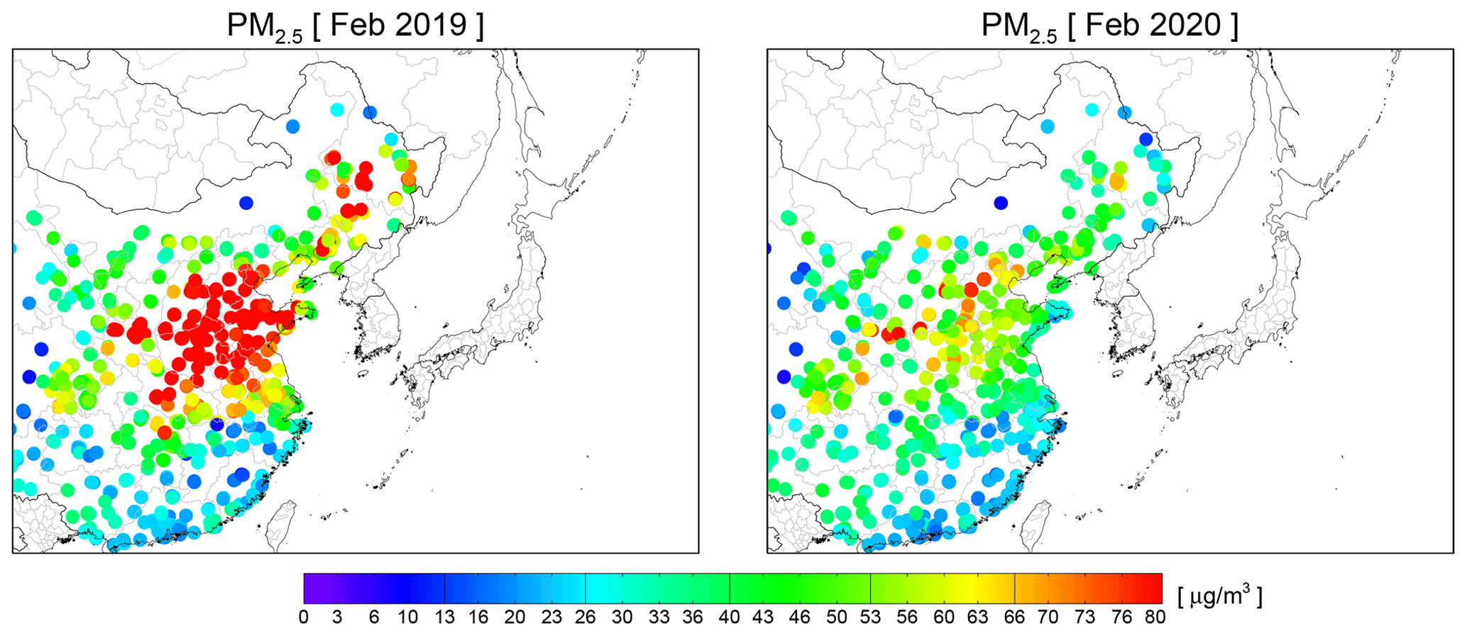
Figure 1 Geographical coverage of modeling domain and surface-monitoring sites. Monthly mean surface PM_2.5 concentrations in February 2019 and February 2020 are shown.

2 Data

2.1 Observations

Surface observation data were obtained from the China National Environmental Monitoring Center (CNEMC; data available at http://www.pm25.in, last access: 25 June 2021). Hourly ambient air concentration data for PM₁₀, PM_2.5, CO, NO₂, O₃, and SO₂ were available for 1571 sites (over China) and 1459 sites (within the study domain; Fig. 1). After removing sites with less than 80 % data availability for each year (2017–2020, ± 60 d of Lunar New Year (LNY)), the analysis used observations from 1332 sites. Data-processing procedures are explained in Sect. 3.1 and further discussed in Sect. 4.4.

2.2 Satellite

The TROPOspheric Monitoring Instrument (TROPOMI) NO₂ vertical column-density, level-2 data (S5P_L2_NO2) were obtained from NASA GES DISC (http://tropomi.gesdisc.eosdis.nasa.gov, last access: 25 June 2021). TROPOMI is a hyperspectral spectrometer onboard the Sentinel-5P satellite, with wavelength coverage over ultraviolet to visible (270 to 495 nm), near infrared (675–775 nm), and shortwave infrared (2305–2385 nm) wavelengths (Eskes et al., 2019; van Geffen et al., 2019). High-quality pixels from level-2 data (3.5 km × 7 km resolution at the nadir) were selected using the quality flags provided by the product (qa_value > 0.75) and then spatially regridded into the study domain using a conservative spatial-regridding method that preserves mass during interpolation (Kim et al., 2018, 2016, 2020).

Table 1 Physical options for meteorological and chemical simulations.

2.3 Model

Meteorological and atmospheric chemistry transport models were used over East Asia with a 27 km horizontal resolution. The Weather Research and Forecasting Model (WRF, version 3.4.1) was used for meteorological simulations (Skamarock and Klemp, 2008). The National Oceanic and Atmospheric Administration (NOAA) National Centers for Environmental Protection (NCEP) Final Analysis (FNL) product (NCEP, 2000) provided the initial and boundary conditions for the WRF simulations. For chemistry simulations, CMAQ (version 4.7.1) (Byun and Schere, 2006), the Meteorology–Chemistry Interface Processor (MCIP, version 3.6) (Otte and Pleim, 2010), and the Sparse Matrix Operator Kernel Emission (SMOKE) modeling framework were used, employing the meteorological inputs provided by the WRF simulations. Table 1 details the modeling configurations, and Fig. S1 in the Supplement compares models with observations. The models provide a reasonably realistic simulation of atmospheric chemical and physical processes over the considered domain, especially in terms of their daily variations from 2017 to 2019 (e.g., R = 0.91 ∼ 0.94 for PM_2.5, see Emery et al. (2017) for general model performance guidance). However, in 2020, as the effects of the pandemic began to take hold, the chemical model's predictions – based on typical (as opposed to pandemic-influenced) emissions – systematically overpredicted pollutant concentrations, consistent with a pandemic-influenced reduction in emissions.

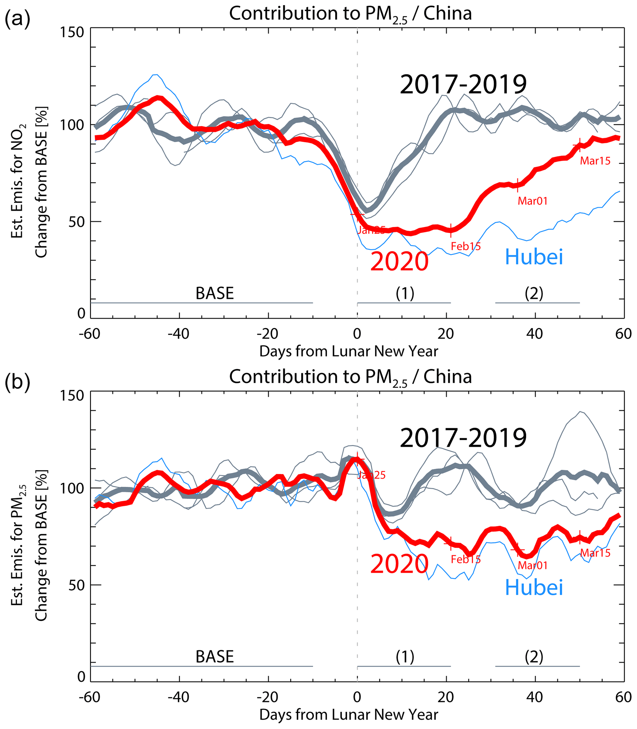
Figure 2 Time series of estimated emissions for (a) NO₂ and (b) PM_2.5 using 1332 surface-monitoring sites across China. The gray lines indicate 2017–2019 variations, with their average in the thick gray line, whereas the red line indicates the 2020 variation. The blue line indicates the 2020 variations in Hubei Province (46 sites). BASE is used as the pre-LNY period, and (1) and (2) denote the period of maximum impact and the recovery period, respectively.

2.4 Emission inventory

This study used two sets of emission inventories, the Comprehensive Regional emission inventory for Atmospheric Transport Experiment (CREATE, version 2.3) (Jang et al., 2020) and the Model Inter-Comparison Study for Asia (MICS-Asia) emission inventory (MIX inventory for the year 2010) (Li et al., 2017). While the CREATE inventory is based on the latest information, including the 2016 KORUS-AQ campaign (https://espo.nasa.gov/korus-aq, last access: 25 June 2021), the MIX inventory has been tested in many diverse applications (J. Li et al., 2019; K. Li et al., 2019; Zhang et al., 2017). The time-series analysis in Fig. 2 (discussed below) was based on the CREATE emission inventory, but the results of the analysis did not depend in any significant way on a choice between these two base inventories. The CREATE inventory is provided as an annual mean for each Chinese province for the year 2016 and the SMOKE preprocessor was used to convert the inventory to hourly model-ready inputs. The base model simulations use these 2016 emissions for the entire 2017–2020 modeling period.

3 Method

This section describes the following aspects of the analysis: (1) data-processing procedures for analyzing the time series, (2) emission adjustment procedures to update SO₂ and NO_x emissions to near real time, and (3) brute-force modeling procedures to estimate Chinese emissions by sector. It should be noted that the time-series analysis (discussed in Sect. 4.1) utilizes fixed emission inventory (i.e., bottom–up emission inventory) and the emission adjustment experiment (Sect. 4.2) utilizes observation-based top–down emissions. The sectoral emission estimation method is for Sect. 4.3.

3.1 Time-series analysis

Four types of variation (meteorological, weekly, yearly, and the Chinese spring festival) were reduced or accounted for in the surface observations, as follows. Meteorological influences were reduced by combining surface data with output from a three-dimensional chemistry model to calculate estimated emissions. Since the model simulations with a fixed emission inventory respond to the variations in meteorological conditions, we can infer the relationship between emissions and ambient pollutant concentrations under specific weather conditions. By applying this relationship, we convert the changes in observed concentrations into the changes in emissions. Weekly variations, a unique feature of anthropogenic emissions, were removed by using a 7 d moving average. The impact of the Chinese spring festival, the biggest traditional holiday celebrating Lunar New Year (LNY), was normalized by rearranging the time series to center on the LNY in each solar year. The LNY alignment was necessary to account for the irregular occurrence of the LNY dates. Seven-day moving average filtering was also required to avoid unfair comparisons between different weekdays after the LNY alignment. Otherwise, we may compare different weekdays for different year (e.g., 2020 LNY on 25 January, Saturday, and 2019 LNY is February 5, Tuesday). Figure S4 shows that the 7 d moving average filter smooths but does not significantly change the time-series results. Finally, yearly emission variations were removed by setting a base period (−60 to −10 d before LNY) and calculating relative changes from the average of the base period.

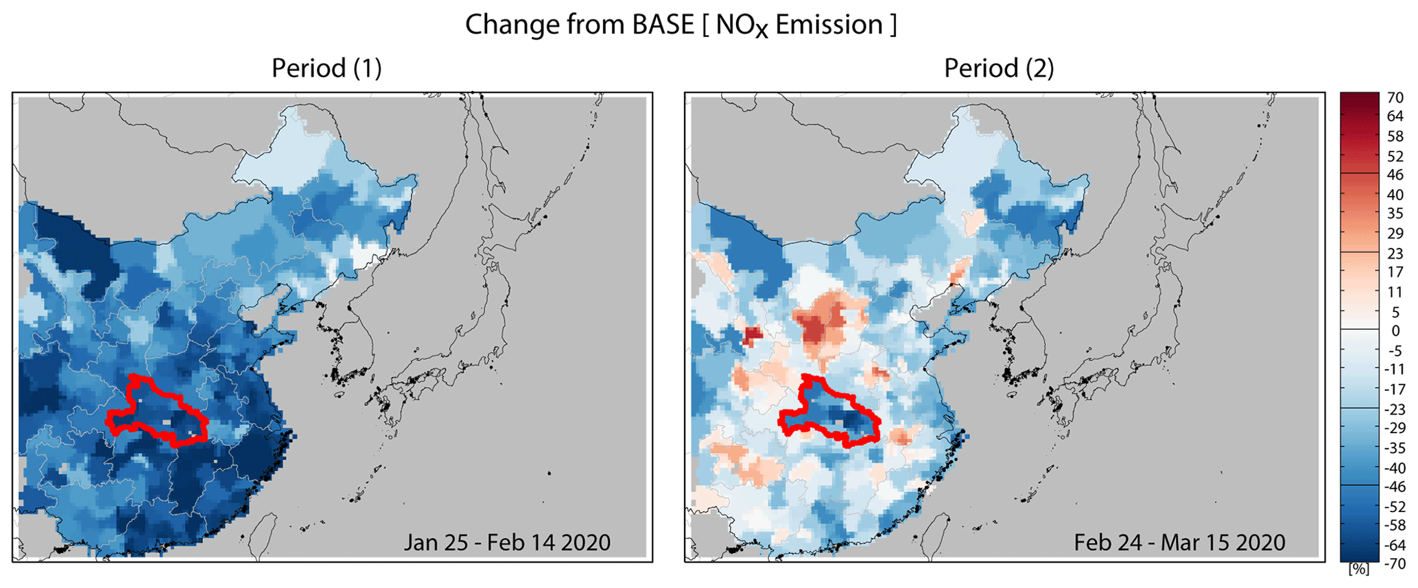
Figure 3 Spatial distribution of the change in estimated NO_x emissions from the baseline period (Fig. 2) during the period of maximum impact (25 January–14 February 2020) and the recovery period (24 February–15 March 2020). Hubei Province is marked in red.

We followed the data-processing procedures suggested by Bae et al. (2020b) for their emissions-updating system (hereafter BAE2020). First, the observational and modeled data were paired and tested, and observation sites with more than 20 % of values missing were discarded. To avoid over-weighting dense urban sites, observations occurring within the same model grid cell were averaged. Second, weekly variations were removed using 7 d moving averages, and the impact of the Chinese spring festival was normalized by rearranging the time series to center on LNY in each year. Third, meteorological variations were removed by applying the ratio between observed and modeled concentrations. Using a simple linear assumption, observed pollutant concentrations were combined with the results of the chemical model to create estimates of actual emissions that are less sensitive to meteorological variations. Use of the linear assumption in the concentration-to-emission conversion is further discussed in Sect. 4.4 The total estimated emissions, E_est, and their relative variations, rE_est, were calculated as

$$\begin{array}{}\text{(1)}& {\displaystyle }{E}_{\text{est}}\left(t\right)=E_{\text{mod}}\cdot {\displaystyle \frac{C_{\text{obs}}\left(t\right)}{C_{\text{mod}}\left(t\right)}},\text{(2)}& {\displaystyle }{\text{rE}}_{\text{est}}\left(t\right)={\displaystyle \frac{E_{\text{est}}\left(t\right)}{\sum _{t=\text{base}}{E}_{\text{est}}\left(t\right)/n_{\text{base}}}}\cdot \mathrm{100}\mathit{\%},\end{array}$$

where C is the daily pollutant concentration; t is days from LNY; base and n_base are the pre-LNY base period (shown in Fig. 2) and its number of days, respectively; and E_mod is the model emissions. To normalize the yearly changes, a base period (−60 to −10 d before LNY) was set, with relative changes calculated from the average of that base period (i.e., rE_est(t)). The impact of the pandemic was inferred by calculating the difference in estimated emissions between normal years and 2020. Since the model uses a fixed emission inventory for each year, E_mod cancels out in the comparison.

Table 2 Comparison of data-processing steps in the emission adjustment methods used in BAE2020 and this study.

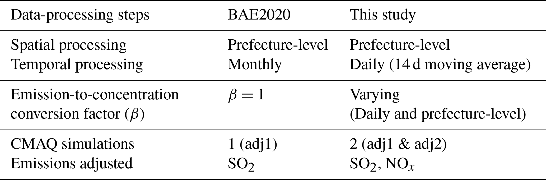
Note: results of “adj1” simulations were used to calculate β values for the “adj2” simulation.

For the spatial analyses of the data (e.g., Fig. 3), point data were converted to area format. Similar to the time-series data processing, the observational and modeled data were paired and tested. Considering the location of each paired data set, we assigned point data to their corresponding Chinese prefecture. By averaging all concentrations in each prefecture, we constructed the prefecture-level concentration data set (for each prefecture polygon), which was then converted into domain grids using a conservative spatial-regridding technique. Section 4.4 further discusses the data-processing procedures.

3.2 Top–down emission adjustment

For the second analysis (discussed in Sect. 4.2), we updated major pollutant emissions to a more realistic level and analyzed simulated chemical behaviors. Due to stringent emission control policies by the Chinese government, Chinese anthropogenic emissions have changed dramatically over recent years. For example, the annual mean surface SO₂ concentration across China was 8.4 ppb in 2016 but dropped to less than half of this level (3.7 ppb) in 2020. To incorporate a realistic change in emissions from 2016 to 2020, we applied observation-based emission adjustment factors to the 2016 CREATE emission inventory to reproduce emissions in 2020. In general, model emissions can be adjusted based on the ratios between observed and modeled surface concentrations:

$$\begin{array}{}\text{(3)}& {\displaystyle \frac{E_{\text{adj}}}{E_{\text{mod}}}}=\mathit{\beta }\cdot {\displaystyle \frac{C_{\text{obs}}}{C_{\text{mod}}}},\end{array}$$

where β is a sensitivity factor in the emission-to-concentration conversion. β is close to 1 if less secondary chemical reactions are involved. BAE2020 assumed a fixed β=1 to update SO₂ emissions, and they demonstrated that the adjusted emissions effectively reproduced surface SO₂ concentrations over China. Similar approaches were also confirmed to be effective for the NO_x emission adjustment over the same East Asian domain using satellite-based measurements of NO₂ column densities (Bae et al., 2020a; Chang et al., 2016).

While this simple assumption works practically, we tried to conduct the emission adjustment processing more carefully, considering the unprecedented changes in the chemical environment during the pandemic period. We extend the approach of BAE2020, offering two major enhancements. First, we calculate daily emission adjustment factors to represent the rapid changes in emissions under the pandemic situation. We applied 14 d moving averages to avoid uncertainties caused by insufficient data points day to day. Second, we calculated spatial and temporal variations in β and then applied these to the emission adjustment factors. Table 2 compares the data-processing steps used in this study with those used in BAE2020.

The β values are calculated as follows. In the real world, the sensitivity of concentration to changes in emissions is not unique or spatially homogeneous (i.e., β≠1), especially for NO_x emissions and NO₂ concentrations. β values for specific location and time can be calculated if we have two model simulations with different emissions applied. Previous studies have calculated β values for a model by using changes in concentration caused by a certain amount of perturbed emissions (e.g., Lamsal et al., 2011, used a 15 % emission perturbation).

To obtain more realistic β values, we have conducted two model simulations: base and adj1 runs. First, the base model simulation was conducted using a normal emission inventory, CREATE, which we have introduced previously. The second simulation, adj1 run, was conducted using perturbed emissions to estimate how the model responds according to the change in emissions. We adjusted emissions according to the ratio between observed and modeled surface concentrations, so we can reproduce a more realistic chemical environment.

From these two simulations, the base and adj1 runs, we calculate the emissions-to-concentration sensitivity, β values, on a specific spatial and temporal scale – for each Chinese prefecture daily. β values are calculated as

$$\begin{array}{}\text{(4)}& {\mathit{\beta }}_{p,t}={\displaystyle \frac{[E_{\text{adj1}}/E_{\text{base}}{]}_{p,t}}{[C_{\text{adj1}}/C_{\text{base}}{]}_{p,t}}},\end{array}$$

where p and t stand for indices of Chinese prefectures and specific dates. Using calculated β values for each prefecture and date, we finally obtain the adjusted emissions for the second and final simulations: the adj2 run.

$$\begin{array}{}\text{(5)}& [E_{\text{adj2}}{]}_{p,t}={\mathit{\beta }}_{p,t}\cdot {\left[{\displaystyle \frac{C_{\text{obs}}}{C_{\text{base}}}}\cdot E_{\text{base}}\right]}_{p,t}\end{array}$$

We further discuss the characteristics of the emissions-to-concentration sensitivity in Sect. 4.4.2.

3.3 Estimation of sectoral contributions

The contributions of emissions from each sector to surface PM_2.5 concentrations over China were estimated using the brute-force method (BFM), an approach that uses changes in modeled outputs as a result of perturbed emission inputs (Burr and Zhang, 2011). The MIX emission inventory provides information on five sectors: residential, industry, power generation, transportation, and agriculture. Sectoral contributions were calculated by applying the perturbed emissions for each sector:

$$\begin{array}{}\text{(6)}& \text{Contr.(sector)}={\displaystyle \frac{(C_{\text{base}}-C_{\mathrm{\Delta }E,\text{sector}})/\mathrm{\Delta }E}{C_{\text{base}}}}\cdot \mathrm{100}\mathit{\%},\end{array}$$

where C is the surface PM_2.5 concentration and ΔE is the ratio of the emission perturbations. A 50 % reduction was chosen to perturb emissions for each individual sector. Fractional contributions of each emission sector were calculated compared to the sum of all five emission sector contributions. The application of the BFM to East Asian air quality models and a discussion of its uncertainties has been presented elsewhere (Kim et al., 2017b).

4 Results

4.1 Time-series analysis

Reducing meteorological, weekly, and yearly variations, as well as variations resulting from the Chinese spring festival made the comparison of pandemic-influenced surface observations to normal conditions more robust and useful. Estimated NO_x emissions (Fig. 2) display variations from the spring festival season. From 2017–2019, the estimated NO_x emissions demonstrate a clear reduction during the festival period (by up to 45 % between −10 and +20 d from LNY). In 2020, this reduction is slightly greater and continues for longer, implying that the coronavirus outbreak further reduced traffic in China. The difference between the estimated emissions in the 2017–2019 time series and those in the 2020 time series in Fig. 2 reflects the relative significance of the impact of the coronavirus (p < 0.01 for t test of comparison after LNY).

Interestingly, the 2020 time series (that is, the combined effect of the spring festival and the coronavirus) remains flat from the LNY to 15 February. As both effects likely overlapped, they appear inseparable during the period. The maximum impact from the coronavirus seen in the data is a 58 % reduction on 15 February 2020 from the level seen in prior, baseline years (2017–2019). The level of NO_x emissions from 1 to 15 February (close to a 50 % reduction) might suggest a floor level for reduced emissions under current conditions in terms of technology and infrastructure. This might have important implications for chemical modeling and emission control, perhaps implying a floor for emission reductions that China can realistically reach under current conditions. The blue line represents a time series from Hubei only (46 sites), showing, as would be expected, that the impact in Hubei has been more significant and sustained.

The reduced NO_x emissions began to increase after 15 February, almost recovering to their normal level by the end of March 2020. Hence, the impact of the coronavirus pandemic on NO_x emissions in China lasted almost 2 months. Figure 3 shows the spatial distribution of the estimated changes in NO_x emissions from the base period to the period of maximum impact (25 January–14 February 2020) and the recovery period (24 February – 15 March 2020). Just after LNY, NO_x emissions strongly reduce across China, but their inferred recovery is spatially inhomogeneous. As shown in Fig. 3, Hubei Province continued to show a strong reduction (by more than 50 %) compared with the pre-LNY level, even in the recovery phase (period 2). Other regions show various patterns in NO_x levels compared with previous years. These observations are consistent with space-borne, remote-sensing measurements from the TROPOMI (Fig. S1). Similar to the surface observations in Fig. 3, the spatial distributions of NO₂ column densities during the period of maximum impact (25 January–14 February) and the recovery period (24 February – 15 March) were generated as changes from the baseline period (26 November 2019–15 January 2020).

The impact of the virus may actually have begun before the spring festival. In normal years (2017–2019), variation in estimated pre-LNY baseline period (−60 to −10 d) NO_x emissions is relatively small because the model uses fixed emissions and weekly variations have already been removed. However, the estimated emissions in 2020 are relatively low, starting from about 15 d before LNY, and this relative reduction is more pronounced in Hubei. This suggests that our baseline period in 2020 already includes a partial coronavirus impact. If this is true, the impact of the pandemic would be even stronger than inferred here, as it is based on a year-by-year comparison of concentrations during and after the typical-year base period.

Unlike the temporal trend in NO_x emissions and their spatial distribution, a comparison of changes in the PM_2.5 level suggests a different story (Fig. 2b). Contrary to NO_x emissions, PM_2.5 concentrations typically show a slight increase near LNY, likely due to increased PM_2.5 emissions from fireworks, a long-held tradition in China (Kong et al., 2015), and show only a relatively moderate reduction from typical levels (by 10 %–20 %) over the remainder of the spring festival. Unlike NO_x emissions, the case of PM_2.5 involves both direct emissions of particulate matter and gas-to-particle conversion of emitted precursors (e.g., SO₂, NO_x, NH₃, VOCs – volatile organic compounds) mediated by atmospheric chemical transformations. As discussed in the Method section, we assume the same approximate relationship for PM_2.5 as with NO_x between the ambient observations and their associated emissions. This approach suggests that emissions decreased by roughly 30 % from normal levels through the end of March to reach 72.7 ± 6.6 % of the 2017–2019 level from 4 February to 25 March 2020. Interestingly, the pandemic does not seem to have significantly affected SO₂ emissions (see Fig. S3), suggesting that the pandemic's effects on the power generation and industrial sectors have been relatively small.

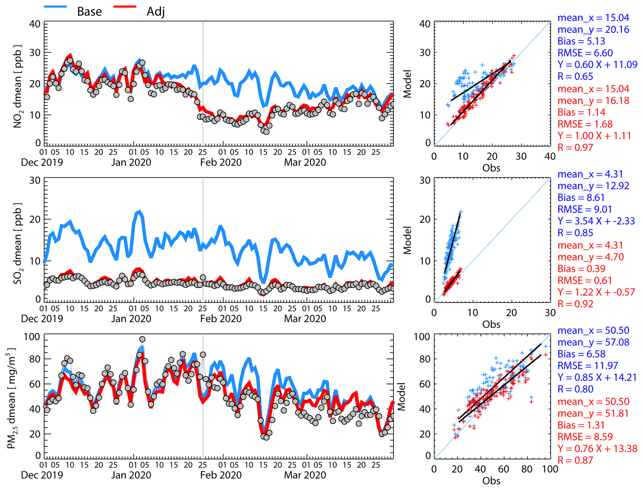
Figure 4 Time series and scatterplots of observed and modeled surface concentrations of SO₂, NO₂, and PM_2.5 from 1332 Chinese surface-monitoring sites during the pandemic period. Model simulations using the baseline emission inventory (CREATE) and top–down adjusted emissions are shown in blue and red, respectively. Observations are represented by gray circles.

4.2 Experiment with updated SO₂ and NO_x emissions

As discussed in Sect. 3.2 above, we used an alternative approach to investigate unidentified PM_2.5 emissions, specifically applying more realistic SO₂ and NO_x emission adjustments. Using this methodology, we repeated CMAQ simulations with SO₂ and NO_x emissions adjusted based on surface measurements. Daily and prefecture-level emission-adjustment factors were calculated and applied to the baseline emission inventory. The two CMAQ simulations – a baseline simulation with the CREATE emission inventory and an adjustment simulation with updated emissions – were both compared with observations from surface-monitoring sites (Fig. 4). Individual site comparisons are also available in Fig. S11.

For both SO₂ and NO₂ concentrations, the CMAQ simulation with adjusted emissions performed well, reproducing observed variations in surface concentrations. It should be noted that the CREATE v2.3 emission inventory we used was constructed for 2016 and applied to a 2020 simulation. Before LNY, simulated NO₂ concentrations with both the baseline and adjusted emission inventory agreed well with observations, implying that there were no significant changes in the NO_x emission level between 2016 and 2020. Near LNY, the baseline NO₂ simulations differ significantly from observations, while the simulation with adjusted emissions successfully reproduced the huge reductions in the LNY and pandemic period. The difference between the baseline and adjusted simulations almost disappears at the end of March, consistent with the result of the time-series analysis (Fig. 2). On the other hand, the baseline SO₂ simulations greatly overestimate observations by 2 or 3 times, implying that nominal, real-world SO₂ emissions in 2020 are much smaller than those reflected in the 2016 emission inventory. By applying the top–down adjustment described here, simulations could successfully reproduce surface SO₂ concentrations, reducing RMSE by 93 % from 9.19 to 0.62 ppb. The updated SO₂ and NO_x emission inventories appear to successfully reproduce variations in surface PM_2.5 concentrations, even after the start of LNY celebrations. However, in early February, as the impact of the COVID-19 pandemic became more significant, the baseline run (with the CREATE emission inventory) does not simulate a sudden drop in PM_2.5 observations, while the adjusted emissions run does so.

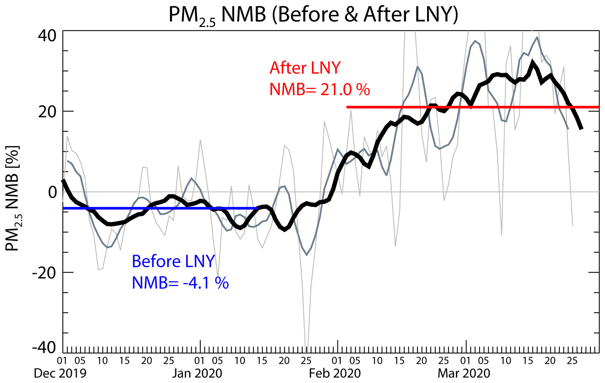
Figure 5 Time series of surface PM_2.5 normalized mean bias during the pandemic period between observed and modeled data with adjusted emissions (i.e., SO₂ and NO_x emissions adjusted). Mean NMBs before and after LNY are also marked. Raw, 7 d, and 14 d moving average NMBs are shown in thin, medium-thin, and thick lines, respectively.

A closer look, however, reveals that the real trend in PM_2.5 emissions cannot be explained by the change in two major inorganic aerosol precursors: SO₂ and NO_x. Figure 5 depicts the time series of normalized mean biases (NMBs) of surface PM_2.5 concentrations. Before LNY, PM_2.5 NMB is mostly negative, showing the adjusted emission simulation slightly underestimates particulate matter. After LNY, PM_2.5 NMB changes prominently, showing the simulation clearly overestimates observations by about 20 % NMB in PM_2.5 concentration. Before and after LNY, PM_2.5 NMB moves by 25.1 %, from −4.1 % to 21.0 %, implying that the model suddenly overestimates PM_2.5 concentrations by 25 % after LNY. In other words, unknown, non-modeled emissions (that is, non-SO₂ and non-NO_x emissions) are clearly reduced enough during the pandemic period (February and March) to account for 25 % of total PM_2.5 concentration at baseline. This result is consistent with findings (Sect. 4.1) that changes in SO₂ and NO_x emissions alone cannot explain the reduced PM_2.5 concentrations in March.

4.3 Sectoral contributions to emissions

One remaining question is why the recovery of NO_x emissions and unchanged SO₂ emissions at the end of March did not lead to the recovery of PM_2.5, which might be explained by considering the time-varying emission contribution of each economic sector. Sensitivity tests using the CMAQ model reveal that the residential and agricultural sectors are most dominant in the early months of the year (Fig. 6), accounting for more than 60 % of surface PM_2.5 concentration over China. As emissions in the residential sector are primarily from cooking and heating with anthracite coal and wood, emissions which continue even during a pandemic, one possible explanation is that emissions from the agricultural sector reduced as a result of pandemic-related delays in planting and fertilizing.

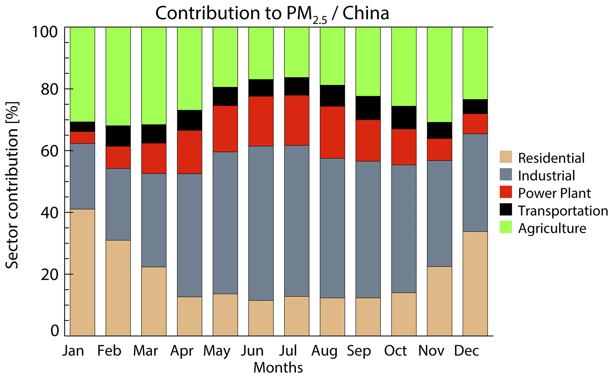
Figure 6 Monthly variations in emission contributions to surface PM_2.5 concentrations over China by sector. The contributions from the five sectors (residential, industry, power generation, transportation, and agriculture) were estimated using a brute-force perturbation method.

February is the start of the spring-crop planting period in southern China. The coronavirus outbreak could have impacted both field crops and livestock farms. Inputs, such as fertilizer and animal feed, have reportedly been scarce as a result of transportation disruptions, and seasonal workers have reportedly been lacking due to quarantine controls or fears (Quanying, 2020; Yu, 2020; Zhang and Xiong, 2020). Agricultural activities that generate particulate matter, such as biomass burning to clear debris and the generation of airborne dust during tilling, are reduced in intensity during the pandemic. Reduced NH₃ emissions as a result of diminished livestock farming activities might also be a factor leading to lower PM_2.5 concentrations.

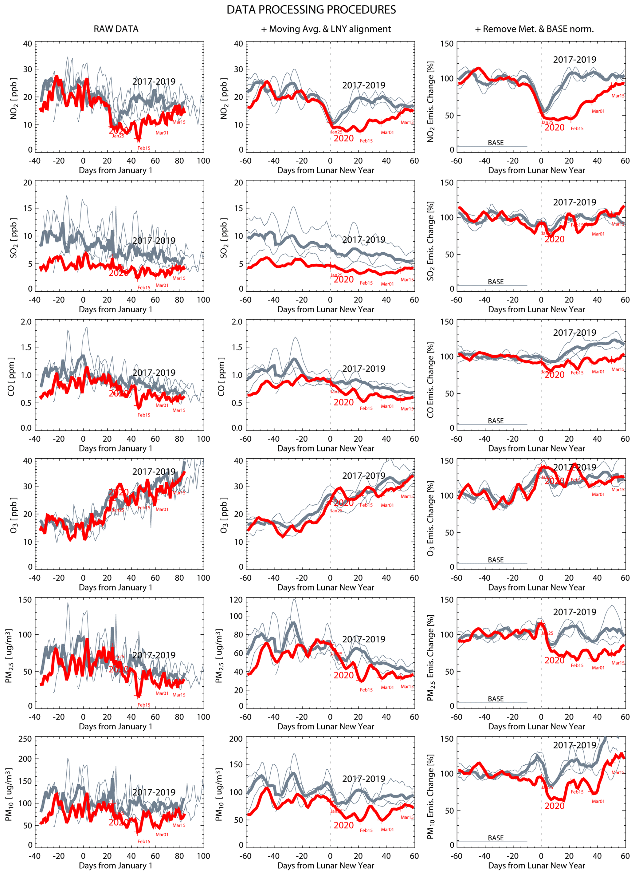
Figure 7 Time series of surface NO₂, SO₂, CO, O₃, PM_2.5, and PM₁₀ concentrations over China following the data-processing procedures step by step. Raw data (left column), data after applying a 7 d moving average and an LNY alignment (middle column), and data after removing meteorological variations and calculating variations from the baseline periods (right column) are all shown.

4.4 Further discussions on the methods

4.4.1 On the data processing of time-series analysis

We further discuss data-processing procedures here. Figure 7 presents a time series of surface pollutants proceeding through data-processing steps. Even in raw format, NO₂ exhibits clear impacts from the pandemic. Impacts on other pollutants (CO, PM₁₀, and PM_2.5), however, are not easily recognizable until confounding signals are fully removed. Interpreting SO₂ concentration data is particularly illuminating. While 2020 SO₂ concentrations are substantially lower than those of previous years, the time series obtained after the data processing described here suggests that SO₂ emissions are mostly consistent before and after LNY. That is, lower SO₂ concentrations in 2020 seem to be a continuation of year-over-year reductions and not a result of the pandemic.

Note that the various instances of linear assumptions used in this analysis should be interpreted with caution especially considering its spatiotemporal resolution and chemical characteristics. Variations in emissions and in chemical and physical processes, including chemical reactions, transport, and dispersion, can create large gradients on local scales that are likely poorly represented in the WRF and CMAQ modeling performed here, even as their importance is somewhat smoothed over regional and nationwide scales. Observed concentrations of a pollutant are generally proportional to the emissions associated with that pollutant; conceptually, a simple linear relationship between emissions and pollutants is assumed. For the pollutants NO₂ and SO₂, these are NO_x and SO₂ emissions, respectively. BAE2020 demonstrated that this concentration-to-emission conversion method can be used effectively at the Chinese prefecture level. Discussion of the spatial representativeness of Chinese surface-monitoring data and associated uncertainties is also presented in BAE2020. For inferring PM_2.5-related emissions, the analysis is more complicated because PM_2.5 results from both primary and secondary (precursor) emissions. While the pollutant–emissions relation for PM_2.5 is nonlinear, especially over relatively small spatial and temporal scales, it is still approximately valid over larger geographical regions and longer time periods.

The validity of the linear assumption was tested through a model sensitivity analysis. A CMAQ simulation with 50 % reduced emissions yielded an approximately 50 % reduction in surface PM_2.5 concentrations over most regions in China (Table S1 in the Supplement). Taken as a whole, surface PM_2.5 concentrations are roughly proportional to overall emissions. Thus, the simplifying assumption of linearity appears reasonable for the more complex PM_2.5 case, generating a time series of estimated pollutant emissions without meteorological variations. Nevertheless, PM_2.5 emissions estimated with this analysis are necessarily more uncertain than are NO_x emissions. Notably, Table S1 also shows that CMAQ simulations with adjustments in SO₂, NO_x, and NH₃ individually showed disproportionately lower responses, suggesting that surface PM_2.5 concentrations are influenced by other emissions (e.g., elemental carbon and organic carbon emissions) and/or nonlinear processes that likely vary with atmospheric chemistry regime.

4.4.2 On the emission adjustment experiment

As stated in the methodology section, we further discuss here the emissions-to-concentration sensitivities (i.e., β). The β values can be calculated using any two model simulations based on different emission inputs, by comparing the change in emissions with the change in simulated concentrations. Furthermore, if we specifically change the emissions according to the ratio of observations and the base model simulation, we further simplify the emission scaling factor as follows.

For this simulation, adj1, if we apply the adjusted emissions using the ratio of the observed and modeled concentrations, the adjusted emissions for the adj1 run, E_adj1, are

$$\begin{array}{}\text{(7)}& E_{\text{adj1}}={\displaystyle \frac{C_{\text{obs}}}{C_{\text{base}}}}\cdot E_{\text{base}}.\end{array}$$

If we apply this to Eq. (4), we can obtain

$$\begin{array}{}\text{(8)}& \mathit{\beta }={\displaystyle \frac{E_{\text{adj1}}/E_{\text{base}}}{C_{\text{adj1}}/C_{\text{base}}}}={\displaystyle \frac{C_{\text{obs}}/C_{\text{base}}}{C_{\text{adj1}}/C_{\text{base}}}}={\displaystyle \frac{C_{\text{obs}}}{C_{\text{adj1}}}}.\end{array}$$

Therefore, the emission adjustment factors in the next simulation (adj2) can be found using Eq. (5):

$$\begin{array}{}\text{(9)}& E_{\text{adj2}}=\mathit{\beta }\cdot {\displaystyle \frac{C_{\text{obs}}}{C_{\text{base}}}}\cdot E_{\text{base}}=\left[{\displaystyle \frac{C_{\text{obs}}}{C_{\text{adj1}}}}\cdot {\displaystyle \frac{C_{\text{obs}}}{C_{\text{base}}}}\right]\cdot E_{\text{base}},\end{array}$$

where adj2 indicates the second and final simulation for the top–down emission adjustment method.

From here, the $\left[\frac{C_{\text{obs}}}{C_{\text{adj1}}}\right]$ term, or β, can be interpreted as an additional adjustment factor to the original adjustment factor in adj1, $\left[\frac{C_{\text{obs}}}{C_{\text{base}}}\right]$. If the emission modification in adj1 results in the same percentage change in concentrations, $C_{\text{obs}}/C_{\text{adj1}}=\mathrm{1}$, we do not need the secondary adjustment. If the simulated concentration from adj1 is smaller (larger) than the observations, we need to increase (reduce) the amounts of emissions. This procedure was applied to create new 2020 emissions of both SO₂ and NO_x.

In most cases, the calculated β values are close to 1 (Fig. S5), implying that the simple assumption β=1 in BAE2020 remains effective. The β values for NO_x emissions are slightly higher than those for SO₂ emissions over polluted areas (Fig. S6), which implies that more secondary reactions are involved in tropospheric NO_x chemistry.

Both enhancements to the top–down simulations – β values and the daily application of emission adjustment factors – clearly improved the model's performance, especially in the pre-LNY periods. While the monthly emission adjustments failed to represent the rapid changes in NO₂ concentrations after 25 January 2020 (Fig. S7), the daily adjustment method successfully modeled these changes (Fig. 4). The general underestimation of NO₂ concentrations was corrected using the β values (Fig. 4). The improved model performance was confirmed by comparing the spatial distributions and scatterplots before and after these adjustments (Figs. S8–S10). Spatial distributions of RMSEs of model performances in SO₂, NO₂, and PM_2.5 are also summarized in Fig. S12.

Understanding the characteristics of the β values in terms of their spatial distribution, temporal variation, and chemical difference is important for several reasons. In the emission update procedure in practice, we can apply the pre-calculated β values from the look-up table if the β values show general consistency according to their location, time, and chemical component. For the emission control policy, the β values provide valuable information on the efficiency of emission control because they suggest how effectively pollutant concentrations can be removed given the amount of emission control by the government.

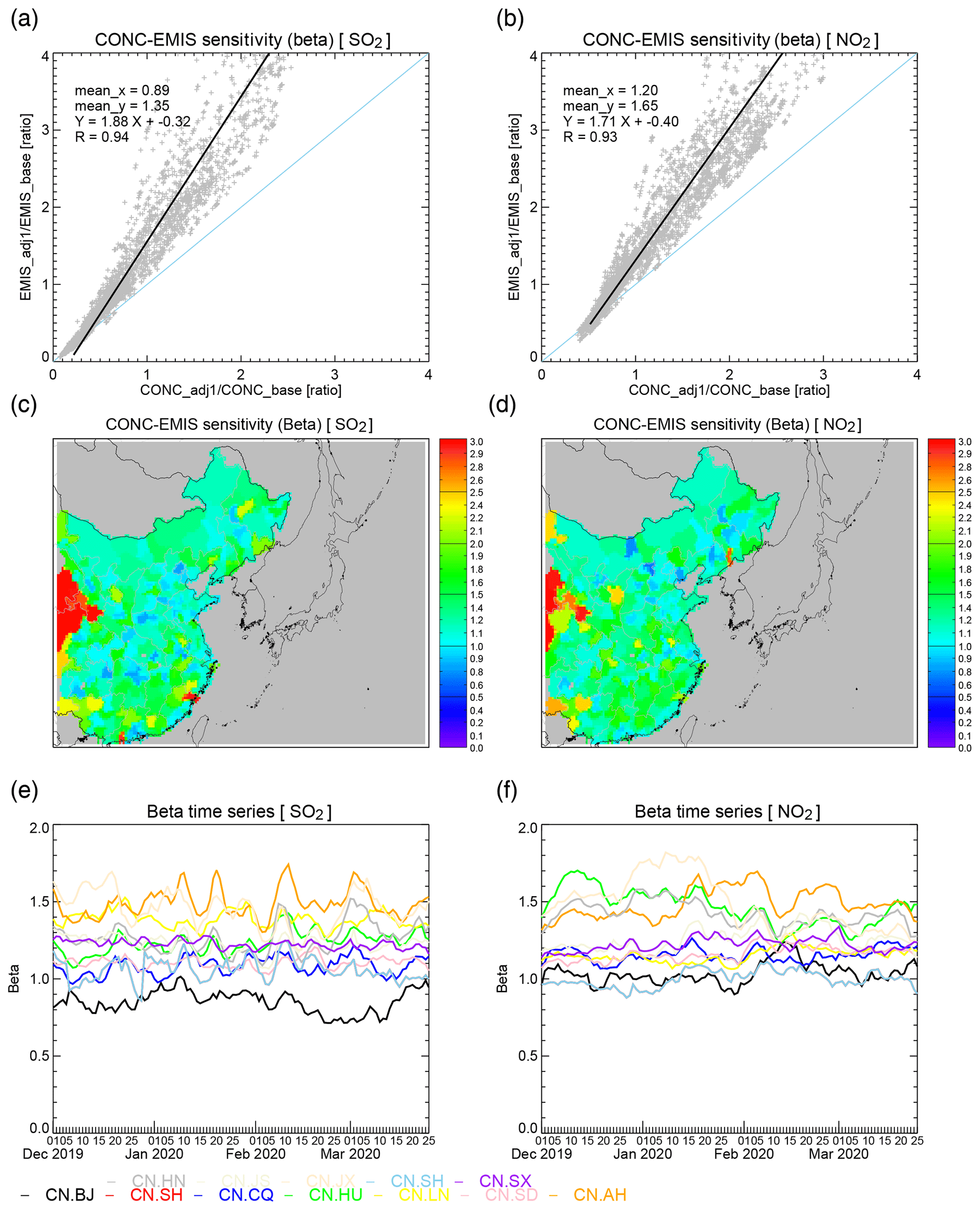
Figure 8 Calculation of the concentration-to-emissions sensitivities (β) for the emission adjustment experiment of SO₂ (left column) and NO₂ (right column). The β values are obtained as the ratio of the emission change (i.e., Emis_adj / Emis_base) to the change in concentrations (i.e., Conc_adj1/Conc_base), which is also consistent with the slope in the scatterplot (a, b). Spatial variations in the average concentration-to-emissions sensitivities (β) during January to March 2020 over China (c, d). The temporal variations in the β values for selected Chinese provinces are shown in the lower panel (e, f). (BJ: Beijing; SH: Shanghai; CQ: Chongqing; HU: Hubei; SD: Shandong; AH: Anhui; HN: Hunan; JS: Jiangsu; SX: Shanxi).

Figure 8 summarizes the characteristics of the β values. As they are defined as the ratio of the emission change (i.e., $E_{\text{adj1}}/E_{\text{base}}$) to the change in concentrations (i.e., $C_{\text{adj1}}/C_{\text{base}}$), the slopes of the fitted lines in the scatterplots describe the emissions-to-concentration sensitivities for SO₂ and NO₂ (Fig. 8a and b). The histogram of the occurrence of the β values also confirms that for both SO₂ and NO₂, the calculated β values are centered slightly over 1 (mean = 1.42 and median = 1.27 for SO₂ and mean = 1.40 and median = 1.26 for NO₂) (Fig. S13). Figure 8c and d demonstrate the spatial distributions of the β values over Chinese territories. Except for a few outside locations, the β values are mostly consistent, around 1. We further investigated the temporal variations in the β values by showing the daily variations in the estimated β values for selected Chinese provinces (Fig. 8e and f). It is evident that the β values differ by location, implying that the emissions-to-concentration sensitivities vary for different regions likely due to their unique chemical and emission environment. However, for each location, the β values are mostly consistent over time. For the practical use of the β values in the emission update procedure, we may use region-specific sensitivity parameterization since their temporal variations over a specific region are not significant.

To evaluate the emission update approach, the key feature in this study is the validation of PM_2.5 concentration. We used observation-based SO₂ and NO₂ emission adjustments, and there was no adjustment in the primary PM_2.5 emissions, meaning that the improvement of PM_2.5 is achieved through chemical reactions and their balances. The surface concentrations of surface PM_2.5 concentrations, especially inorganic aerosols, are formed by secondary reactions, which are determined by the balance of chemical reactions for nitrate, sulfate, and ammonium. The performance of the PM_2.5 simulations provides strong evidence that the top–down emission adjustment method used in this study is valid and successfully reproduces a realistic chemical environment.

Formation efficiency of sulfate aerosols by updating SO₂ and NO_x emission is also very interesting. From Fig. 4, one may notice that the change in total PM_2.5 concentration is not prominent in the pre-pandemic period, even with strong reduction in SO₂ emissions. Modeled PM speciation components show that the reduced sulfate concentrations were canceled out by the increased nitrate concentrations, due to the balance of nonlinear nitrate–sulfate–ammonium chemistry. Nitrate is the most dominant component of PM_2.5 during the wintertime (contributing ∼ 50 % while sulfate contributes 14 %), and the sudden drop of PM_2.5 concentrations during the pandemic is mostly driven by the change in nitrate concentrations. This result implies an important message to emission control policy, suggesting that both SO₂ and NO_x emission reductions will be required to achieve better emission reduction efficiency.

5 Summary

We investigated changes in observed surface pollutant concentrations and precursor emissions over China and inferred changes in human activity as a result of the coronavirus pandemic. Three analyses were conducted: (1) a time-series analysis, (2) an emission adjustment experiment, and (3) sectoral emission contribution estimations. First, we removed four types of variation (meteorological, weekly, yearly, and the LNY) to isolate impacts of coronavirus pandemic from observed surface pollutant concentrations. A chemistry model simulation with fixed emission inventory was used to remove meteorological variations. The analysis has shown that NO_x emissions across China recovered to almost normal levels 2 months after LNY. However, considering the estimated changes in emissions associated with PM_2.5, some emissions remain missing, as of the end of March 2020, compared with normal years. Second, an alternative modeling approach using updated real-time SO₂ and NO_x emissions also suggested that about 25 % of PM_2.5 emissions are likely missing from the period. Third, impacts of sectoral emissions were presented to infer the role potential missing emissions or activities.

The surface observations of pollutants and inferred precursor emissions across China suggest that the country is recovering, as evidenced by the apparent resumption of near-normal transportation-related emissions. The pandemic appears not to have strongly affected the industrial sector; continued depression in estimated PM_2.5-associated emissions may be due to effects on the agricultural sector. If the sustained reduction in PM_2.5 is due to reduced activity in the agricultural sector, agricultural production could be affected, at least in the short term. This could hold important implications for China's path to recovery and, potentially, for broader parts of the world if similar types of agricultural impacts occur elsewhere.

The data analysis approach used here has attempted to isolate the ambient data signal due to the coronavirus from other sources of variation. The apparent difference between the recovery timelines for NO₂ and PM_2.5 suggests that estimating NO_x emissions alone is insufficient to draw conclusions about the overall recovery of the Chinese economy. Overall, changes in concentrations of atmospheric pollutants can provide useful information about the spatial and temporal economic impacts of the coronavirus pandemic, a serious global issue.