the Creative Commons Attribution 4.0 License.
the Creative Commons Attribution 4.0 License.
 | 06 Jul 2021
Anthropogenic and natural controls on atmospheric δ13C-CO2 variations in the Yangtze River delta: insights from a carbon isotope modeling framework
Cheng Hu
Jiaping Xu
Cheng Liu
Yan Chen
Dong Yang
Wenjing Huang
Lichen Deng
Shoudong Liu
Timothy J. Griffis
Xuhui Lee
The atmospheric carbon dioxide (CO2) mixing ratio and its carbon isotope (δ13C-CO2) composition contain important CO2 sink and source information spanning from ecosystem to global scales. The observation and simulation for both CO2 and δ13C-CO2 can be used to constrain regional emissions and better understand the anthropogenic and natural mechanisms that control δ13C-CO2 variations. Such work remains rare for urban environments, especially megacities. Here, we used near-continuous CO2 and δ13C-CO2 measurements, from September 2013 to August 2015, and inverse modeling to constrain the CO2 budget and investigate the main factors that dominated δ13C-CO2 variations for the Yangtze River delta (YRD) region, one of the largest anthropogenic CO2 hotspots and densely populated regions in China. We used the WRF-STILT model framework with category-specified EDGAR v4.3.2 CO2 inventories to simulate hourly CO2 mixing ratios and δ13C-CO2, evaluated these simulations with observations, and constrained the total anthropogenic CO2 emission. We show that (1) top-down and bottom-up estimates of anthropogenic CO2 emissions agreed well (bias < 6 %) on an annual basis, (2) the WRF-STILT model can generally reproduce the observed diel and seasonal atmospheric δ13C-CO2 variations, and (3) anthropogenic CO2 emissions played a much larger role than ecosystems in controlling the δ13C-CO2 seasonality. When excluding ecosystem respiration and photosynthetic discrimination in the YRD area, δ13C-CO2 seasonality increased from 1.53 ‰ to 1.66 ‰. (4) Atmospheric transport processes in summer amplified the cement CO2 enhancement proportions in the YRD area, which dominated monthly δs (the mixture of δ13C-CO2 from all regional end-members) variations. These findings show that the combination of long-term atmospheric carbon isotope observations and inverse modeling can provide a powerful constraint on the carbon cycle of these complex megacities.
- Article
(15281 KB) - Full-text XML
-
Supplement
(1314 KB) - BibTeX
- EndNote


Urban landscapes account for 70 % of global CO2 emissions and represent less than 3 % of Earth's land area (Seto et al., 2014). Such CO2 hotspots play a dominant role in controlling the rise in atmospheric CO2 concentrations, which exceeded 412 ppm in December 2019 for global monthly average observations (https://www.esrl.noaa.gov/gmd/ccgg/trends/, last access: 1 August 2020). Furthermore, the carbon isotope ratio of CO2 (i.e., δ13C = 13C 12C ratio in delta notation) at the representative Mauna Loa site, USA, has steadily decreased to around −8.5 ‰ in December 2019 (https://www.esrl.noaa.gov/, last access: 1 August 2020). Anthropogenic CO2 emission is produced from fossil fuel burning and cement production. As the urban population is expected to increase by 2.5 to 6 billion people in 2050, anthropogenic CO2 emissions are projected to increase dramatically, especially in developing regions and countries (Sargent et al., 2018; Ribeiro et al., 2019). Under such a scenario, the observations of atmospheric CO2 and δ13C-CO2 in urban landscapes are of great importance to monitoring these potential CO2 emissions hotspots (Lauvaux et al., 2016; Nathan et al., 2018; Graven et al., 2018; Pillai et al., 2016; Staufer et al., 2016).
Countries are required to report their CO2 emissions according to the Intergovernmental Panel on Climate Change guidelines (IPCC, 2019), and many bottom-up methods have long been used to estimate CO2 emissions worldwide, but such methods have high uncertainties for CO2 emissions at regional (20 %) to city (50 % to 250 %) scales (Gately and Hutyra, 2017; Gately et al., 2015). These large uncertainties are propagated into the estimation of biological fluxes in atmospheric inversions (Zhang et al., 2014; Jiang et al., 2014; Thompson et al., 2016). By using CO2 observations, the top-down atmospheric inversion approach is a useful tool to evaluate bottom-up inventories (Graven et al., 2018; L. Hu et al., 2019; Lauvaux et al., 2016; Nathan et al., 2018). Previous research has shown that additional information, such as data on atmospheric Δ14CO2-CO2, δ13C-CO2, and CO, is needed to better distinguish CO2 emissions from different sources and to assess their uncertainties (Chen et al., 2017; Graven et al., 2018; Nathan et al., 2018; Cui et al., 2019). The use of hourly δ13C-CO2 observation in urban areas remains rare in inversion studies, yet such observations contain invaluable information of anthropogenic CO2 from different categories.
Traditional estimates of δ13C-CO2 using isotope ratio mass spectrometry (IRMS) are very limited because flask air sample collection requires long preparation time and is expensive. Consequently, there is a lack of high temporal and long-term observations of δ13C-CO2 (Sturm et al., 2006). Isotope ratio infrared spectroscopy (IRIS) technology has overcome these limitations. As a result, in situ air sample analyses using IRIS analyzers result in dense time series of δ13C-CO2. However, most of the established long-term IRMS and IRIS δ13C-CO2 measurement sites are representative of “background”, natural, or agricultural ecosystems at locations far away from urban landscapes (Chen et al., 2017; Griffis, 2013).
To date, long-term (> 1-year) and continuous observations of both CO2 and δ13C-CO2 have been reported for only five cities, including Bern, Switzerland (Sturm et al., 2006), Boston, USA (McManus et al., 2010), Salt Lake City, USA (Pataki et al., 2006), Beijing, China (Pang et al., 2016), and Nanjing, China (Xu et al., 2017). In these previous investigations, significant diel and seasonal variations of δ13C-CO2 have been observed; these patterns were modulated by fossil fuel combustion, plant respiration and photosynthesis, and changes in the height of the atmospheric boundary layer (Sturm et al., 2006; Guha and Ghosh, 2010). No study has quantified the impact of each factor on the seasonal variation of δ13C-CO2. This represents an important knowledge gap in understanding the underlying mechanisms of carbon cycling in complex urban ecosystems.
The traditional δ13C-CO2 isotope partitioning methods (including the Miller–Tans and Keeling plot approaches) have been used to constrain different CO2 sources worldwide (Keeling, 1960; Vardag et al., 2015; Newman et al., 2016; Pang et al., 2016; Xu et al., 2017). These methods are based on the assumption that partitioned atmospheric CO2 enhancement components from different sources can represent CO2 emissions in the “target area” (Miller et al., 2003; Ballantyne et al., 2011). Carbon dioxide emissions are highly inhomogeneous at the urban scale, with extremely strong point/line sources, and the final partitioning results are highly uncertain without considerations of source footprint characteristics (Gately and Hutyra, 2017; Cui et al., 2019; Martin et al., 2019). Atmospheric transport models can help to resolve such problems, and the coupling of atmospheric transport models with isotope observations has recently been applied in global and regional CO2 partitioning studies (Chen et al., 2017; Cui et al., 2019; Graven et al., 2018; Hu et al., 2018b). Although urban CO2 inversions have been applied successfully in several studies in Europe and the United States (Bréon et al., 2015; Turnbull et al., 2015; Pillai et al., 2016; Brioude et al., 2013; Turner et al., 2016), urban CO2 inversions in China are rare (Berezin et al., 2013; Hu et al., 2018a; Worden et al., 2012), presumably because of the scarcity of high-quality δ13C-CO2 and CO2 observations.
The Yangtze River delta (YRD) ranks as one of the most densely populated regions in the world and is an important anthropogenic CO2 hotspot. Major anthropogenic sources include the power industry, oil refineries/transformation and cement production. Having the largest source of cement-derived CO2 production across China and the world (Cai et al., 2015), the YRD contributed 20 % of national cement production, nearly 12 % of the world's total cement output in 2014 (USGS, 2014; Xu et al., 2017; Yang et al., 2017). In addition to anthropogenic factors, natural ecosystems and croplands act as significant CO2 sinks and sources within the YRD. Independent quantification of the fossil and cement CO2 emission and assessment of their impact on atmospheric δ13C-CO2 have the potential to improve our understanding of urban CO2 cycling. Further, the observations and simulations of both atmospheric CO2 and δ13C-CO2 can help us relate atmospheric CO2 dynamics to future emission control strategies.
Here, we combine long-term (>2-year) CO2 and δ13C-CO2 observations with atmospheric transport model simulations to study urban atmospheric CO2 and δ13C-CO2 variations. The objectives were to (1) constrain anthropogenic CO2 emissions and determine the main sources of uncertainty for δ13C-CO2 simulations and (2) quantify the relative contributions of each factor (i.e., background, anthropogenic CO2 emissions especially for cement production, ecosystem photosynthesis and respiration) to seasonal variations of atmospheric δ13C-CO2.
2.1 Observations of atmospheric CO2 mixing ratio, δ13C-CO2 and supporting variables
The observation site is located on the Nanjing University of Information Science and Technology campus (hereafter NUIST, 32∘12′ N, 118∘43′ E; green dot in Fig. 1a). Continuous atmospheric CO2 mixing ratios and δ13C-CO2 were measured at a height of 34 m above ground with an IRIS analyzer (model G1101-i, Picarro Inc., Sunnyvale, CA). The observation period extended from September 2013 to August 2015. Calibrations for CO2 mixing ratio and δ13C-CO2 were conducted with standard gases traceable to NOAA/GML (NOAA Global Monitoring Laboratory) standards. Calibration details are provided by Xu et al. (2017). Based on Allan variance analyses, the hourly precisions of CO2 and δ13C-CO2 were 0.07 ppm and 0.05 ‰, respectively. We note that the δ13C-CO2 IRIS (model G1101-i) measurements are sensitive to water vapor concentration. Sensitivity tests reveal that the δ13C-CO2 IRIS measurements are biased high (less than 0.74 ‰) when water vapor mole fraction exceeds 2 %. The data presented here have been corrected following the procedures outlined in Xu et al. (2017).
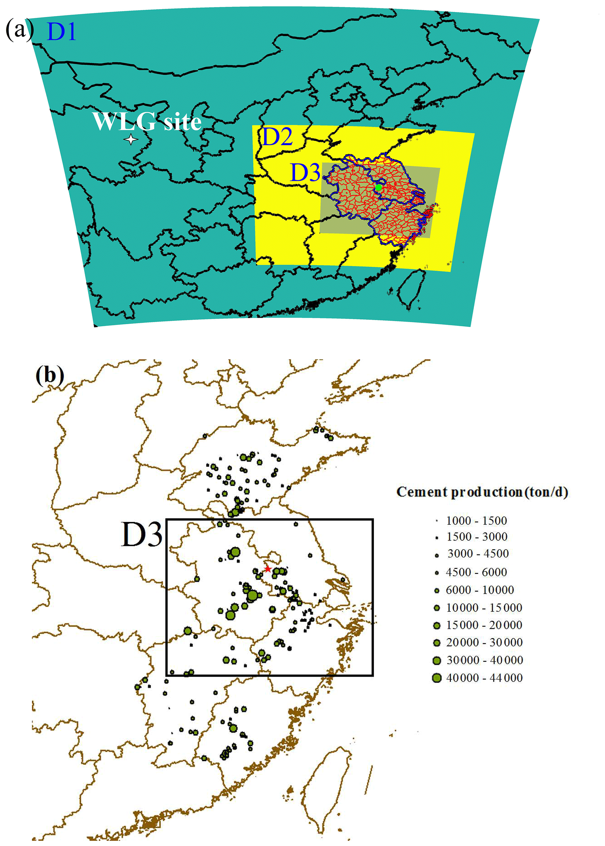
Figure 1(a) Weather Research and Forecasting Model simulation domains and the location of the WLG site; the different region colors represent three domains. (b) Cement production distribution in the YRD and eastern China. Both the green dot in (a) and the red star in (b) are the NUIST observation site.
We separated the 2-year study period into seasons (autumn: September, October, November; winter: December, January, February; spring: March, April, May; summer: June, July, August). Further, for an annual comparison, we examined the period from September 2013 to August 2014 (year 2014) versus September 2014 to August 2015 (year 2015).
The YRD is a cement production hotspot in China (Fig. 1b). It had a total population of 190 million in 2018 (Fig. 2a), with 24.2 million in the city of Shanghai, 9.8 million in Hangzhou (provincial capital of Zhejiang), 8.4 million in Nanjing (provincial capital of Jiangsu), and 8.1 million in Hefei (provincial capital of Anhui). The CO2-related production data (i.e., cement) and energy consumption data (i.e., coal and natural gas) were obtained from local official sources using the same method described in Shen et al. (2014).
To examine the effects of plant photosynthesis on atmospheric CO2 variations, we used the NDVI (Normalized Difference Vegetation Index), SIF (solar-induced chlorophyll fluorescence) and GPP (gross primary productivity) information. These three products have a global distribution with a spatial resolution of 0.05∘ by 0.05∘. The NDVI has a temporal resolution of 16 d, and SIF and GPP products have a temporal resolution of 8 d (Li and Xiao, 2019; http://globalecology.unh.edu/data/, last access: 5 March 2020). Land-use and land-cover classification in the Yangtze River delta for 2014 was applied by using NDVI data from MOD13A2.
2.2 Simulation of atmospheric δ13C-CO2
2.2.1 General equations
The simulation of atmospheric δ13C-CO2 is based on mass conservation. First, we briefly describe the simulation of atmospheric CO2 mixing ratios (more details are provided in Sect. 2.2.2), following the previous work of Hu et al. (2018b), where atmospheric CO2 was simulated (CO2_sim) as the sum of background (CO2_bg) and the contribution from all regional sources/sinks ([ΔCO2_sim]i), as
Note that ΔCO2 is the sum of all simulated sources/sinks [ΔCO2_sim]i and represents the total simulated CO2 enhancement. We use ΔCO2_obs as the observed CO2 total enhancement, which can be calculated by using the CO2 observation minus the CO2 background values. Based on mass conservation, we estimated the 13CO2 composition by multiplying the left- and right-hand sides of Eq. (1) by δ13C:
where δ13Ca_sim and δ13Cbg represent the simulated atmospheric δ13C-CO2 and background δ13CO2, and is the δ13C-CO2 for end-member i (including anthropogenic and biological source categories). The δ13C-CO2 contributions from all regional sources/sinks can be further reformatted as Eq. (3):
where δs_sim is the simulated enhancement-weighted mean of all regional end-members. We use δs as the observed term to distinguish it from δs_sim (Newman et al., 2008), which will be described in detail in Sect. 2.2.5. The product on the right-hand side of Eq. (3) is the simulated regional source term that is added to the background value and contains both enhancement and δ13C-CO2 signals contributed by different CO2 sources/sinks. This product can also be treated as an observed term when using the derived δs_obs and observed δCO2_obs values.
To date, there are no available global δ13C-CO2 background products, and the choice of δ13Cbg is essential for simulating δ13Ca. Here, we apply three strategies. First, we used discrete δ13C-CO2 flask observations at Mount Waliguan (hereafter WLG, 36∘17′ N, 100∘54′ E; https://www.esrl.noaa.gov/gmd/dv/data/, last access: 31 December 2019) to represent the δ13C-CO2 background signal at our site. These observations were measured at weekly intervals to the end of 2015. A digital filtering curve-fitting (CCGCRV) regression method was applied to derive hourly background values following Thoning et al. (1989). There are, however, reasons why WLG may not be an ideal background site for our study domain. For example, based on the previous simulation results for the CO2 background sources, most of the back trajectories originate from the free atmosphere or 1000 m higher above the ground (C. Hu et al., 2019). Further, the footprint at the northern/western edge of domain 1 is relatively small, indicating that most back trajectories were observed above the planetary boundary layer height (hereafter PBLH). Here, the WLG observations were made near the surface. Further, WLG is not located at the border of our simulation domain 1. Therefore, the strong vertical δ13C-CO2 gradients between the boundary layer and the free tropospheric atmosphere (Chen et al., 2006; Guha and Gosh, 2010; Sturm et al., 2013) can cause a low bias in the δ13C-CO2 background when using this approach.
In the second approach, the δ13C-CO2 background signal was estimated with wintertime “clean” air CO2 and δ13C-CO2 observations at the NUIST site, using the following equation:
where δ13Ca and CO2 represent atmospheric δ13C-CO2 and CO2 observations at the NUIST site under clean conditions. Note that δ13Ca represents the observed δ13C-CO2, not the simulated δ13C-CO2 (δ13Ca_sim) as shown in Eq. (2). [ΔCO2_sim]i is the simulated category-specified CO2 enhancements. We defined clean conditions as the bottom 5 % wintertime CO2 observations to minimize simulated CO2 enhancement errors from both biological and anthropogenic CO2 simulations on δ13C-CO2 background calculation. The CO2_bg is obtained from heights 1000 m above ground level (see Sect. 2.2.3).
In the third approach, we avoid the use of modeled [ΔCO2_sim]i results and replaced the simulated regional source term in Eq. 4 with observed δs_obs×CO2_obs, as described in Eq. (3), and used the Miller–Tans regression method to calculate monthly δs_obs. This approach does not require simulation of [ΔCO2]i or the corresponding δ13C-CO2 signals. The hourly δ13C-CO2 background value can be derived by using δs_obs, CO2 background, observed atmospheric δ13Ca and CO2 (see details in Sect. 2.3 and the Supplement). Comparison of these three strategies will be evaluated and discussed in Sect. 3.2.1. Similar methods used to derive other background tracers have included CO2 (Alden et al., 2016; Verhulst et al., 2017), CO (Wang et al., 2010; Ruckstuhl et al., 2012) and CH4 (Zhao et al., 2009; Verhulst et al., 2017; C. Hu et al., 2019). To analyze the controlling factors for the δ13C-CO2 seasonality, the CCGCRV (a digital filtering curve-fitting program developed by the Carbon Cycle Group, NOAA, USA) regression was applied to the background, observations, and simulations. Finally, we derived CCGCRV curve-fitting lines by using 11 regressed parameters, which were based on the hourly time series of observations/simulations, and defined the difference between peak and trough in 1 year as the seasonality of δ13C-CO2.
2.2.2 Simulation of atmospheric CO2 mixing ratios
In Eq. (1), the CO2_bg is obtained from the Carbon Tracker 2016 product, which provides global CO2 distributions from the ground level up to a height of 50 km. We used the averaged concentration above the latitude and longitude where the released particles entered study domain 1 (Fig. 1a). The variable ΔCO2_sim was derived by multiplying the simulated hourly footprint function by the hourly CO2 fluxes (Hu et al., 2018a, b). Considering the diurnal variations of both anthropogenic and biological CO2 fluxes, 168 footprints were obtained representing each simulated hour. This accounted for the back trajectory of particle movement for 168 h (i.e., 24 h per day for 7 d) of transport. The 168 footprints are multiplied by the corresponding hourly CO2 flux. The CO2 fluxes contain anthropogenic CO2 emissions, biological CO2 flux and biomass burning. Here the anthropogenic CO2 emission sources include the power industry, combustion for manufacturing, non-metallic mineral production (cement), oil refineries/transformation industry, energy for building and road transportation. Theoretically, ΔCO2_sim represents the CO2 changes contributed by every pixel within the simulated domain. As shown by Hu et al. (2018a), most of the ΔCO2_sim is contributed by sink/source activity within the YRD area. In order to quantify the relative contributions within the YRD area, we separated the study domain into five zones based on provincial administrative boundaries including Jiangsu, Anhui, Zhejiang, Shanghai, and the remaining area outside the YRD (Fig. 2). The modeled CO2 was calculated as follows:
where fluxi (units: mol m−2 s−1) corresponds to each CO2 flux category simulated for each domain for a specific hour i, and footprint (units: ppm m2 s µmol−1) is the model-simulated sensitivity of observed CO2 enhancement to flux changes in each pixel. The i contains the hourly footprint during the trajectory of particle movement for 168 h as described above. The CO2 enhancements from each of the five zones were simulated by multiplying CO2 emissions in each province by the corresponding footprint.
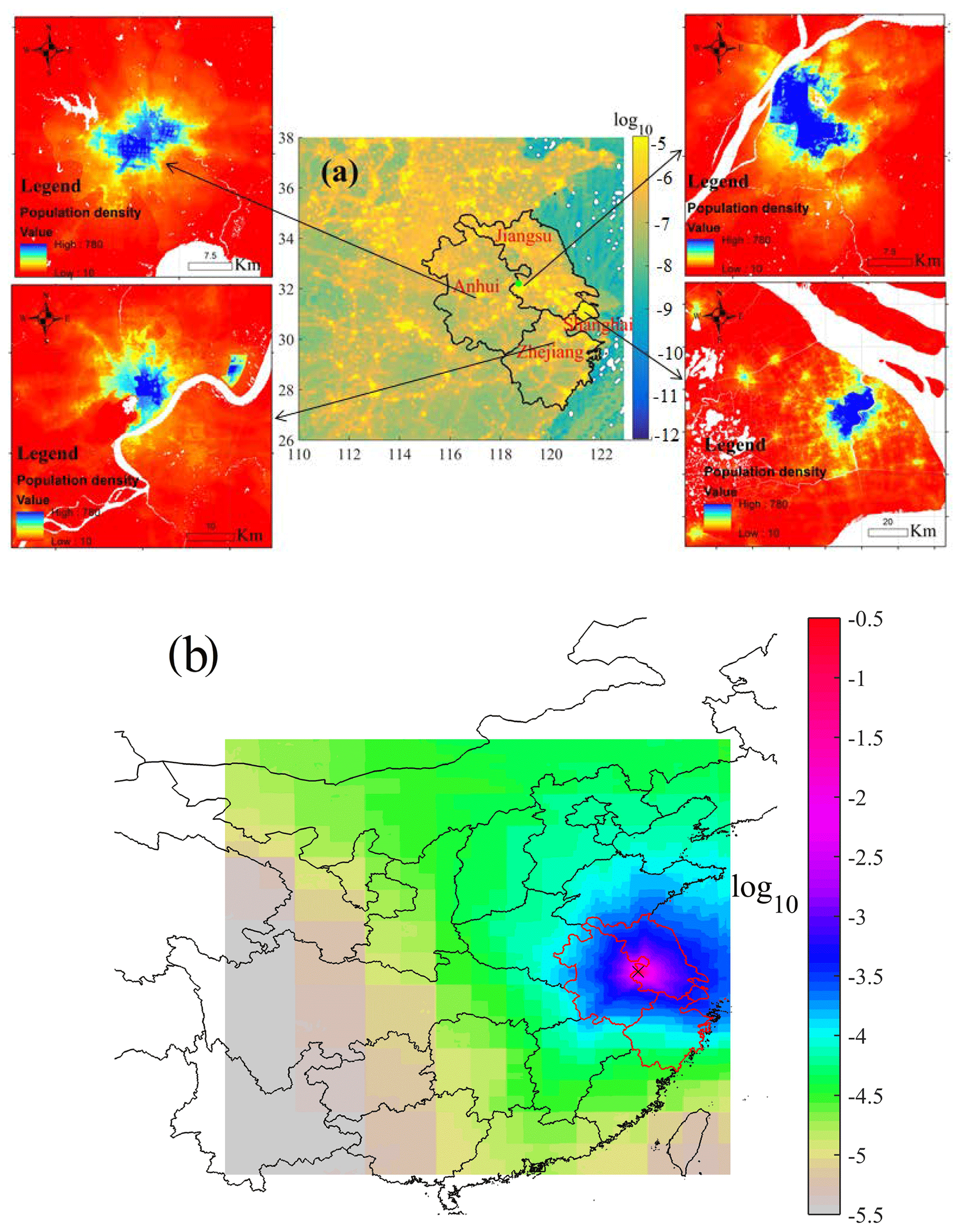
Figure 2(a) Annual anthropogenic CO2 emissions for the study domain (units: mol m−2 s−1) and population density in four megacities (units: people per hectare) including Nanjing, Hefei, Zhejiang, and Shanghai for the year of 2015 and (b) the 2-year average concentration footprint (units: ppm m2 s mol−1).
2.2.3 WRF-STILT model configuration
The Stochastic Time-Inverted Lagrangian Transport (hereafter STILT) model was used to generate the above footprint, which is defined as the sensitivity of atmospheric CO2 enhancement to the upwind flux at the receptor site (observation site). The meteorological fields used to drive the STILT model were simulated with the Weather Research and Forecasting Model (WRF3.5) at high spatial and temporal resolutions. The innermost nested domain (D3, 3 km × 3 km, Fig. 1) contains the YRD area, where the most sensitive footprint is located, and the intermediate domain (D2, 9 km × 9 km) and outermost domain (D1, 27 km × 27 km) represent eastern China and central and eastern China, respectively. The same physical schemes and parameter setup for the WRF meteorological field simulation and the domain in the STILT model have been used previously for inverse analyses (C. Hu et al., 2019). These previous studies at the NUIST observation site have shown very good performance in simulating the meteorological fields, which is essential for reliable STILT simulations. The hourly footprint was simulated by releasing 500 particles from the NUIST measurement site and tracking their backward locations every 5 min for a period of 7 d. Particle numbers and their residence time within half of the PBLH were used to calculate the footprint over the 7 d period. For the CO2 background of each hour, we tracked the sources of air particles' back trajectory for 7 d and defined these CO2 mixing ratios in Carbon Tracker as the hourly CO2 background values (Peters et al., 2007).
2.2.4 A priori anthropogenic CO2 emissions and net ecosystem exchange
The Emission Database for Global Atmospheric Research (EDGAR v4.3.2) inventory was selected as the a priori anthropogenic CO2 emissions (Fig. 2a), which is based on the International Energy Agency's (IEA's) energy budget statistics and provides detailed CO2 source maps (29 categories, including both organic and fossil emissions, IEA, 2012) with global coverage at high spatial resolution (0.1∘ × 0.1∘). The EDGAR CO2 emissions are the most up-to-date global inventory with sectoral detail (Janssens-Maenhout et al., 2017; Schneising et al., 2013). Other inventories, including the Fossil Fuel Data Assimilation System (FFDAS, Rayner et al., 2010) and the Open-source Data Inventory for Anthropogenic CO2 (ODIAC, Oda et al., 2018), also provide global CO2 emissions. However, these inventories only provide total CO2 emissions or have very limited emission categories, which limits our ability to provide isotope end-member information. EDGAR v4.3.2 provides emission estimates at a monthly timescale. Here, we applied hourly scaling factors for different categories following Hu et al. (2018a). EDGAR v4.3.2 with monthly resolution is available only for 2010. We assume that each CO2 category changes linearly from its 2010 value (Peters et al., 2007) and apply an annual scaling factor of 1.145 to derive CO2 emissions for 2014 and 2015. This scaling factor is based on Carbon Tracker, dividing the same anthropogenic CO2 emissions for the YRD in years 2014–2015 by that in 2010.
The biological flux or net ecosystem CO2 exchange (NEE) and biomass burning CO2 emissions come from Carbon Tracker a posteriori flux at 3 h intervals and at a spatial resolution of 1∘ × 1∘. Because NEE is much smaller than the anthropogenic CO2 emissions in such densely developed urban landscapes, we homogeneously distributed this flux at a spatial resolution of 0.1∘ within each grid to match the footprint.
2.2.5 Simulation of the carbon isotope ratio of all sources (δs_sim)
The carbon isotope ratio of all the surface sources was calculated as (Newman et al., 2008)
where δi is the δ13C-CO2 value from source category i, and pi is the corresponding enhancement proportion (i.e., proportions of a specific enhancement i to total CO2 enhancement). We define δs_sim as the simulated carbon isotope ratio of all sources to differentiate it from the observed δs_obs. Based on fossil fuel usage characteristics in the YRD, we reassigned the EDGAR v4.3.2 categories according to fuel types. Coal was the fuel type for manufacturing, oil for oil refinery, natural gas for buildings, and diesel and gasoline for transportation. The power industry consumed 5 % natural gas and 95 % coal based on local activity data in the YRD (State Statistical Bureau, 2016). The non-metallic mineral production was mainly for cement. Since there is a lack of detailed information for non-metallic mineral production, we simply attributed 100 % of it to cement production. Chemical processes were mainly ammonia synthesis. Based on a literature review and our previous work (Xu et al., 2017), typical δ13C-CO2 values for natural gas (−39.06 ‰ ± 1.07 ‰), coal (−25.46 ‰ ± 0.39 ‰), fuel oil (−29.32 ‰ ± 0.15 ‰), gasoline (−28.69 ‰ ± 0.50 ‰), ammonia synthesis (−28.18 ‰ ± 0.55 ‰), diesel (−28.93 ‰ ± 0.26 ‰), pig iron (−24.90 ‰ ± 0.40 ‰), crude steel (−25.28 ‰ ± 0.40 ‰), cement (0 ‰ ± 0.30 ‰), and biofuel combustion and biological emissions (−28.20 ‰ ± 1.00 ‰) were used in this study. We also applied a value of −28.20 ‰ for photosynthesis (Griffis et al., 2008; Lai et al., 2014) because the YRD is a region dominated by C3 plants. Since CO2 emissions associated with human respiration (Prairie and Duarte, 2007; Turnbull et al., 2015; Miller et al., 2020) are relatively small (3.7 % of anthropogenic emissions in the YRD area, Xu et al., 2017) and given that the local food diet is dominated by C3 grains that have a similar δ13C-CO2 value to the biological CO2 flux of −28.20 ‰, we assume it has the same isotope signals as local C3 plants and ecosystem respiration. Further, the biological CO2 flux from the Carbon Tracker assimilation system considered anthropogenic emissions to be fixed and attributed the remainder to the biological CO2 flux (Peters et al., 2007). Consequently, we believe the uncertainty in the biological CO2 flux will include the small proportion of human respiration.
To evaluate the simulated δs_sim, we applied the Miller–Tans and Keeling plot approaches to derive δs_obs from the observed concentration and atmospheric 13CO2-CO2 (Xu et al., 2017). We then used the results to evaluate the calculations made with Eq. (6).
2.3 Independent IPCC method for anthropogenic CO2 emissions
Large differences among inventories have been previously found even for the same region (Berezin et al., 2013; Andrew, 2018). For comparison with the EDGAR v4.3.2 inventory results, we derived the anthropogenic CO2 emissions by using an independent IPCC method. Here, we illustrate the calculation for cement CO2 emissions. Note that the IPCC only recommended an EF for clinker, which is an intermediate product of cement. To calculate cement CO2 emissions, we need to calculate it based on clinker production, as shown in Eq. (7):
where CO2 [cement] is the chemical process CO2 emissions for cement production, Mcement is the production of cement, Cclinker represents the clinker-to-cement ratio (%), and EFclinker is the CO2 emission factor for clinker production. The IPCC recommended an EFclinker value of 0.52±0.01 t CO2 per tonne clinker produced, where CaO content for clinker is assumed to be 65 % with 100 % CaO from calcium carbonate material (IPCC, 2019). The EF appears to be well constrained, showing little variation among provinces with mean values ranging from 0.512 to 0.525 (Yang et al., 2017). For the Cclinker values, it generally showed a decreasing trend from 64.5 % in 2004 to 56.9 % in 2015 for all of China (Fig. S1 in the Supplement), with an average value of 57.0 % during 2014 and 2015.
2.4 Multiplicative scaling factor method
To quantify anthropogenic CO2 emissions and to compare them with EDGAR products, we first derived the monthly scaling factors for anthropogenic CO2 emissions using a multiplicative scaling factor (hereafter MSF) method (Sargent et al., 2018; He et al., 2020) and then obtained annual averages. The monthly scaling factors (SFs) were calculated as
where CO2_obs, ΔCO2_bio, ΔCO2_fire and ΔCO2_anthro represent observed CO2 mixing ratios, simulated CO2 enhancements contributed by biological flux, biomass burning, and anthropogenic emissions, respectively. Uncertainties of all factors on the final MSFs were calculated based on Monte Carlo methods, where the normal sample probability distribution was applied and the upper 97.5 % and lower 2.5 % of the values were considered to be the uncertainty for MSF (Cao et al., 2016).
3.1 Evaluation of hourly CO2 mixing ratios
3.1.1 Hourly and monthly CO2 mixing ratio comparisons
This section examines the general performance of simulating hourly CO2 mixing ratios. The 2-year average hourly footprint is shown in Fig. 2b, where the source area (blue–red) indicates strong sensitivity of the CO2 observations to regional sources. This footprint shape is representative of the YRD area. To quantify the relative contributions from each province, we calculated CO2 enhancements contributed by Anhui, Jiangsu, Zhejiang, Shanghai, and the remaining area outside of the YRD, respectively. The results indicate that Jiangsu contributed approximately 80 % of the total enhancement (discussed further in Sect. 3.1.2). Comparisons between simulated and observed hourly CO2 mixing ratios are displayed in Fig. 3a for both years. For all hourly data in each year, the model versus observation correlation coefficient (R) was R=0.38 (n=8204, P<0.001) and RMSE = 29.44 ppm for 2014 and R= 0.35 (n=7262, P<0.001) and RMSE = 30.22 ppm for 2015. These results indicate that the model can simulate the synoptic and diel CO2 variations over the 2-year period. The model also captured the monthly and seasonal variations of CO2 mixing ratios (daily averages are shown in Fig. S2). The simulations captured the trend of rising CO2 mixing ratios after October and the drawdown of CO2 to the background value during the summer.
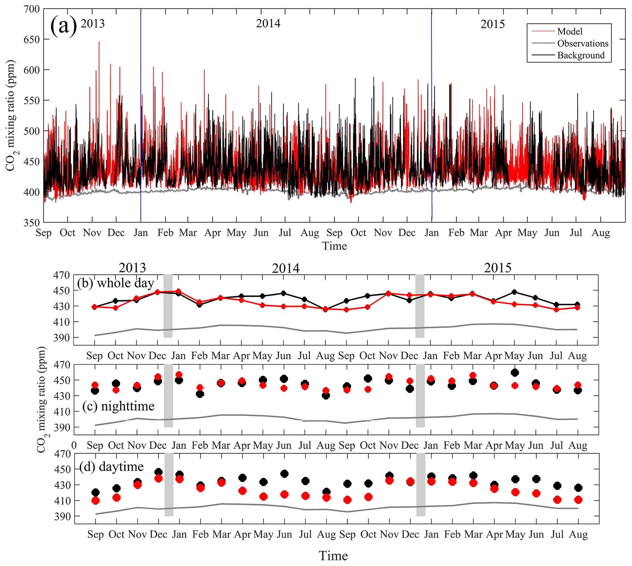
Figure 3(a) Comparisons of hourly CO2 mixing ratios between observations and model simulation from September 2013 to August 2015 and monthly averages for (b) whole day, (c) nighttime (22:00–06:00, local time) and (d) daytime (10:00–16:00). Model results (red), observations (black), and background (grey).
Figure 3b–d illustrate the average monthly daily, nighttime (22:00–06:00, local time), and daytime (10:00–16:00) CO2 mixing ratios. These monthly values contain the effects of atmospheric transport, background and variations in CO2 emissions. The observed and simulated CO2 mixing ratios showed a significant increase from September 2013 to January 2014. Here, the CO2 mixing ratios increased by 16.0 ppm according to the model results and 17.2 ppm according to the observations. The background values increased by 8.1 ppm and accounted for 47 % of the total CO2 increase, and the net CO2 flux (a priori) for the YRD increased by 15 %. We attributed the remaining 38 % increase to changes in atmospheric transport processes including lower PBLH in January 2014 than in September 2013. To quantify how variations in PBLH affected CO2 mixing ratios, we compared the simulated monthly anthropogenic CO2 enhancement differences in the same months of different years to eliminate the influence of monthly emission variations on CO2 enhancements. Twelve monthly paired values were used and are shown in Fig. 4. This analysis indicates that atmospheric CO2 mixing ratios decreased by about 3.7 ppm for an increase in PBLH by 100 m. We also note that there were 2 months (March and August) that fall far below this trend, implying that changes in the monthly footprints (source area) can also play an important role.

Figure 4Relation between monthly PBLH and change in the CO2 mixing ratio; here, these dots represent the difference of monthly averages in 2 different years for all hours.
On an annual timescale, the simulated average CO2 mixing ratios were 436.63 and 437.11 ppm for 2014 and 2015, respectively. Since the anthropogenic CO2 emissions used in the model are the same for both years, the simulated annual average CO2 difference can be used to quantify the influence associated with meteorological factors and ecosystem carbon cycling. Between these 2 years, the CO2 background increased by 1.78 ppm, and the biological enhancement decreased by 1.04 ppm from 2014 to 2015. The remaining 0.26 ppm change between 2014 and 2015 indicates a relatively small meteorological effect for the annual averages, such as a slight change in the dominant wind direction or a PBLH difference.
The simulated annual average NEE CO2 enhancements were 2.64 and 1.60 ppm for the respective years. For comparison, the annual average anthropogenic enhancements were 36.20 and 34.90 ppm for 2014 and 2015, respectively. The monthly NEE enhancement varied from −0.1 ppm in May 2015 to +6.0 ppm in July 2014, indicating NEE contributes positively for enhancement in most months (Fig. 5a), even though the sign of the monthly averaged NEE flux in summer was negative (sinks). This positive contribution was mainly caused by diel PBLH variations between daytime (smaller negative enhancement) and nighttime (larger positive enhancement). To further evaluate the impact of plant photosynthetic activity on the regional CO2 cycle, we examined the NDVI, SIF and GPP seasonal patterns (Fig. 5d–f). These three datasets revealed two peaks during each year, which is related to increased photosynthetic activity. The first peak occurred in May and the second in August–September, corresponding to the growing season of wheat and corn/rice, respectively (Deng et al., 2015). We note that GPP was derived from SIF, and as a result, they share a similar seasonal cycle. The land-use classification in the YRD for 2014 (Fig. S3) shows that the northern YRD is dominated by agricultural land and the south dominated by forest land, and our observation site was more surrounded by agricultural land, which corresponded well to observed NDVI, SIF and GPP seasonal patterns. The peak SIF and GPP signals during the summer were about 20 times greater than during the winter. Consequently, we can ignore the potential influence of photosynthetic activity on the regional CO2 enhancements during the non-growing seasons.
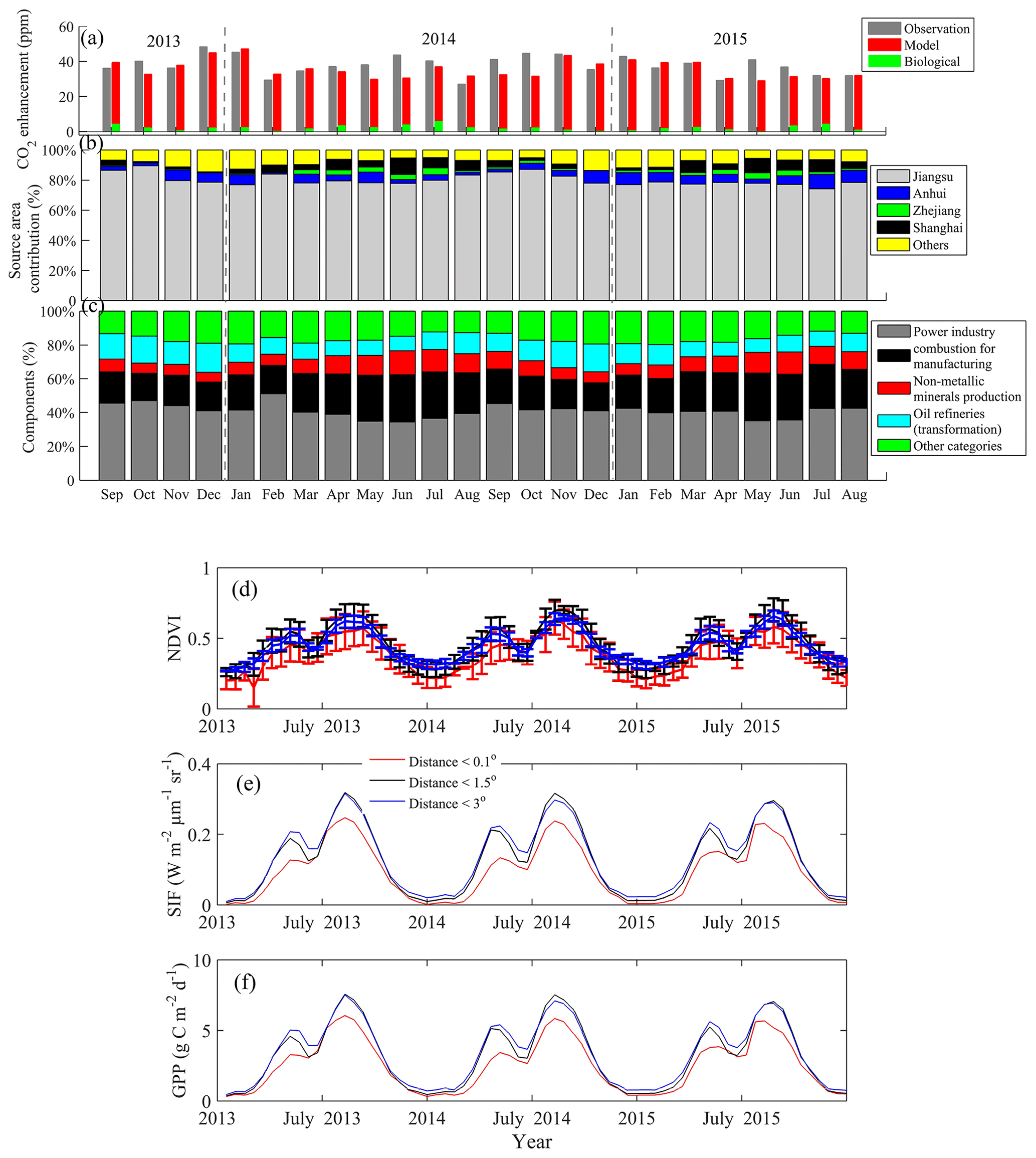
Figure 5(a) Comparisons of simulated and observed CO2 enhancement; note that “model” represents the sum of both anthropogenic and biological CO2 enhancement simulations, (b) CO2 enhancement contributions from different provinces, and (c) simulated anthropogenic CO2 enhancement proportion for the main sources. Time series (2013 to 2015) of (d) NDVI, (e) SIF, and (f) GPP. The distance indicates the radius of the area centered with the NUIST observation site, and the NDVI, SIF, and GPP values are averages in these areas.
3.1.2 Components of urban CO2 enhancement
Here, we diagnose the source contributions to the urban CO2 enhancement. The observed anthropogenic CO2 enhancements, which were derived by subtracting CO2 background and simulated biological enhancement from CO2 concentration observations, were 38.36 ± 3.32 and 37.89 ± 2.80 ppm for 2014 and 2015, respectively. Here, the uncertainty of the observed anthropogenic CO2 enhancements was calculated by prescribing a 2 ppm potential bias for the Carbon Tracker CO2 fields and 50 % to the simulated biological CO2 enhancement (Hu et al., 2018b). The corresponding simulated anthropogenic CO2 enhancements were 36.20 and 34.90 ppm. In comparison with the simulated biological CO2 enhancements displayed in Fig. 5a, both the observed and simulated CO2 enhancements are indicative of a large anthropogenic (fossil fuel and cement production) CO2 emission from the YRD.
Previous studies have also investigated urban CO2 enhancements from a relatively broad range of developed environments worldwide. Verhulst et al. (2017) measured CO2 mixing ratios at seven sites in Los Angeles, USA, and concluded that the mean annual enhancement varied between 2.0 and 30.8 ppm, which is considerably lower than our findings. Another study in Washington DC, USA, in February and July 2013 showed that the CO2 enhancement was less than 20 ppm (Mueller et al., 2018). The urban CO2 observations and modeling study by Martin et al. (2019) at three urban sites in the eastern USA showed an enhancement of ∼ 21 ppm in February 2013, substantially lower (by ∼ 20 ppm) than our observations. The measurements at an urban–industrial complex site in Rotterdam, Netherlands, indicated a CO2 enhancement of only 11 ppm for October to December 2014 (Super et al., 2017). Our enhancements were significantly higher than all of these previous reports of other urban areas.
The anthropogenic components and source area contributions are displayed in Fig. 5b–c. During the study period the average anthropogenic enhancements were 5.1 %, 80.2 %, 1.9 %, 4.4 %, and 8.5 % for Anhui, Jiangsu, Zhejiang, Shanghai, and the remaining area outside the YRD, respectively. Although Shanghai's area is the smallest within the YRD region and relatively distant (∼ 300 km) from our observation site, its maximum source contribution at times exceeded 50 % (i.e., on 19 September 2013, not shown) via long-distance transport. In general, the power industry, manufacturing, non-metallic mineral production, oil refinery, and other source categories contributed 41.0 %, 21.9 %, 9.3 %, 11.5 %, and 16.3 % to the total anthropogenic CO2 enhancement, respectively. The proportions of corresponding CO2 emission categories to the total anthropogenic emissions of the YRD were 39.8 %, 28.4 %, 7.4 %, 4.1 %, and 24.4 %, respectively. The comparisons between the proportions of simulated enhancement and proportions of corresponding CO2 emissions can illustrate whether CO2 enhancement partitions are a good tracer for emissions in a complex urban area. We found a relatively large difference between the enhancement proportion and the emission proportion for oil refineries (from 11.5 % to 4.1 %) as compared to other categories. This may be because the power industry, manufacturing and non-metallic mineral production were more homogeneously distributed compared to oil refineries, which were closer to our CO2 observation site. Further, changes in source footprint caused by wind direction variations likely played an important role.
3.1.3 Constraints on monthly anthropogenic CO2 emissions
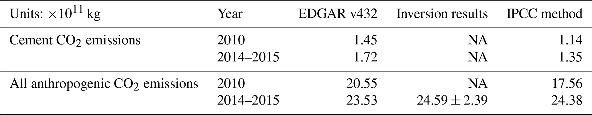
To provide a robust comparison of bottom-up CO2 emissions for the YRD, we calculated anthropogenic CO2 emissions from both EDGAR v4.3.2 and with activity data provided by local governments (Table 1) and the default IPCC emission factors (https://www.ipcc-nggip.iges.or.jp/EFDB/, last access: 13 September 2019). The total anthropogenic CO2 emissions in 2014–2015 were 24.4 × 10¹¹ and 23.5 × 10¹¹ kg according to our own inventory and EDGAR v4.3.2 CO2, respectively, indicating excellent agreement (within 4 %) between these approaches. We constrained the monthly anthropogenic CO2 emissions by using the MSF method (Eq. 8) and computed the 12-month average to represent the years of 2014 and 2015. The a posteriori results indicate that the annual scaling factors were 1.03 ± 0.10 for 2014 and 1.06 ± 0.09 for 2015. The monthly scaling factors derived from using daytime and all-day observations are also shown in Fig. S4. These factors vary seasonally, with higher values observed in summer. When using daytime values only, the scaling factors were much larger than the all-day values. This can be seen in Fig. 3 by comparing the simulated and observed CO2 mixing ratios. We should note here that the larger scaling factors based on the daytime data could be caused by bias in the a priori daily scaling factors used to generate the hourly CO2 emissions (Hu et al., 2018b), the monthly anthropogenic averages, and bias in negative biological CO2 enhancement. Since our study is mainly focused on the seasonality of all-day observations, the monthly scaling factors derived from the all-day approach will be used for the following analyses. The anthropogenic CO2 emissions in year 2015 did not show a significant change compared to 2014, and the overall estimates were within the uncertainty of the estimates. After applying the average scaling factors for 2014 and 2015, the a posteriori anthropogenic CO2 emissions were 24.6 (± 2.4) × 1011 kg for the YRD area. The application of the MSF method provides an overall constraint on the anthropogenic CO2 emissions (also displayed in Table 1).
Table 1Comparisons of cement and all anthropogenic CO2 emissions among the different methods. “NA” means not available.
The main uncertainties associated with the simulation of hourly CO2 and δ13C-CO2 are uncertainty in meteorological fields, transport model (i.e., number of released particles), and a priori CO2 fluxes. At the annual scale the main uncertainty is attributed to the PBLH simulations and a priori anthropogenic CO2 emissions. The anthropogenic CO2 emissions biases were < 6 % as described above, and the bias associated with PBLH uncertainty was typically < 13 % (Hu et al., 2018a, b). There, we attribute a 20 % uncertainty to the simulated CO2 and δ13C-CO2 signals on an annual timescale.
3.2 Simulation of atmospheric δ13C-CO2
3.2.1 Background atmospheric δ13C-CO2
To obtain the best representative δ13C-CO2 background value for the study domain, we examined the values from the three strategies described above (Fig. 6). We also compared the δ13C-CO2 at the WLG background site with observations at NUIST during winters (Fig. S5). This was performed to help simplify the comparison by removing the effects of plant photosynthetic discrimination. The δ13C-CO2 at the WLG site was relatively more depleted in the heavy carbon isotope (or negative, by up to 0.5 ‰) than that observed at NUIST for many periods. Theoretically, there are two key factors that can cause the urban atmospheric δ13C-CO2 to be relatively more enriched in the heavy carbon isotope (or positive) compared to the background values, including (1) discrimination associated with ecosystem photosynthesis and (2) enrichment of the isotopic signature associated with the CO2 derived from cement production. As shown earlier, the biological CO2 enhancement was positive in winter, which implies a positive biological CO2 signal where ecosystem respiration is more important than photosynthesis. Further, sensitivity tests for cement CO2 sources showed its influence is much smaller than the observed difference in Fig. S5 (discussed in Sect. 3.3.3). Based on the above analyses and methods introduced in Sect. 2.3, we concluded that the WLG δ13C-CO2 signal is not an ideal choice for representing the background value. The wintertime δ13C-CO2 background values, based on strategy 2, were −7.78 ‰ and −7.61 ‰ for 2013–2014 and 2014–2015, respectively (Fig. 6). The corresponding values, based on strategy 3, were −7.70 ‰ and −7.53 ‰. These background values are more enriched compared to the WLG observations by 0.80 ‰ to 1.01 ‰. These derived values agree well with the monthly δ13C-CO2 simulation results of Chen et al. (2006), who showed that δ13C-CO2 is 0.6 ‰ higher above the PBL than in the surface layer near the ground. Recently, Ghasemifard et al. (2019) showed that hourly δ13C-CO2 values at the Zugspitze, the highest (2650 m) mountain in Germany, varied between −7 ‰ and −12 ‰ in the winter for 2013. During two especially clean air events (in October and February) at the Zugspitze, the δ13C-CO2 was approximately −7 ‰, during which the CO2 mixing ratios varied between 390 and 395 ppm. This is consistent with our estimates using strategies 2 and 3. Based on the evidence presented above, we believe that strategy 3 is the most robust way to derive a background δ13C-CO2 for the study domain.
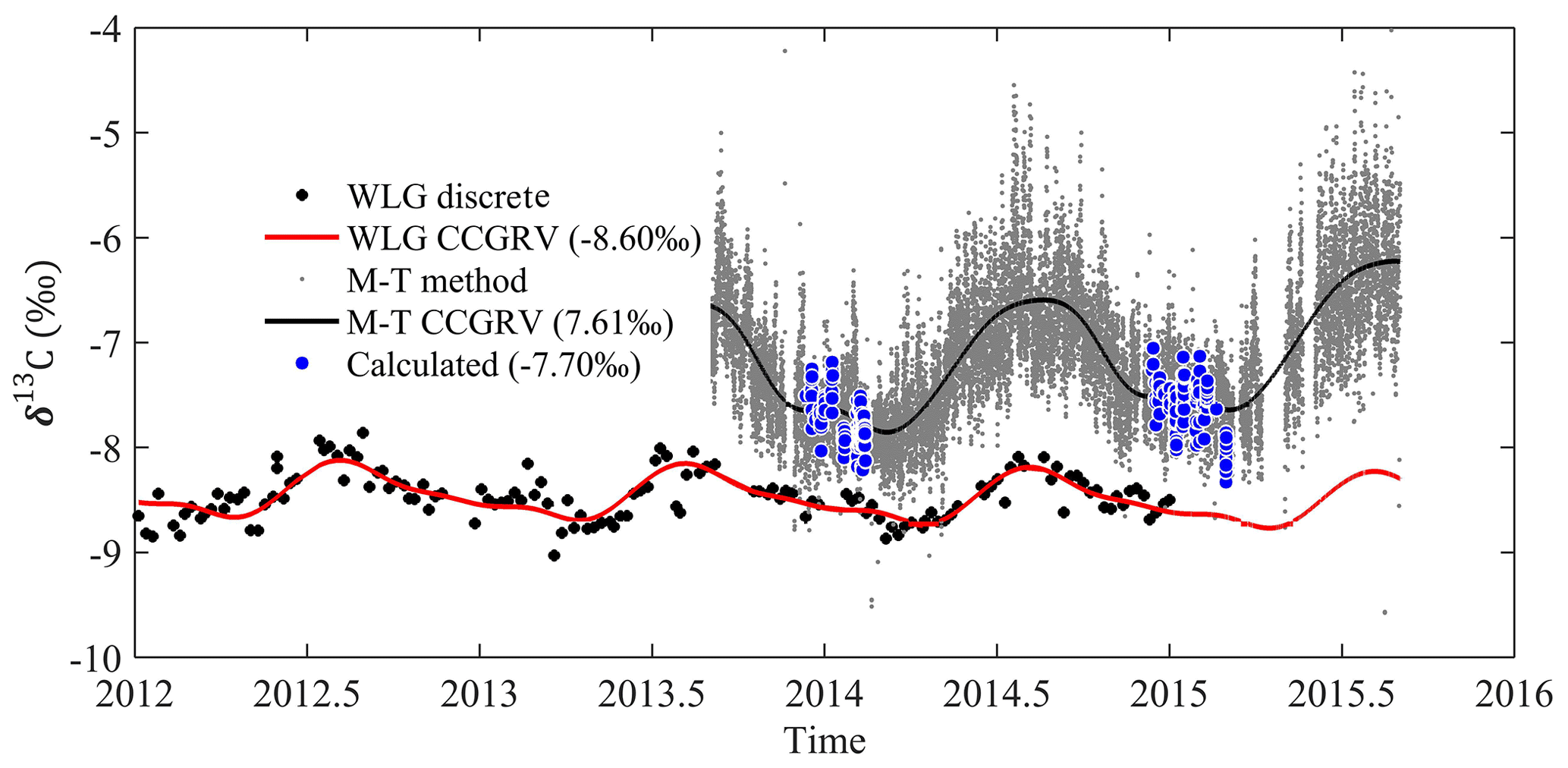
Figure 6Comparisons among three strategies for calculating the background δ13C-CO2. Strategy 1 (WLG discrete: weekly discrete observations at the WLG site, WLG CCGCRV: derived hourly data with WLG observations and CCGCRV method), strategy 2 (calculated by choosing clean air in winter), and strategy 3 (M-T method: derived results with observations and M-T approach, M-T CCGCRV: derived hourly results with the M-T approach and CCGCRV method; see details in Sect. 2.2.1).
3.2.2 Evaluation of δ13C-CO2 simulations
Figure 7a shows the hourly δ13C-CO2 simulations over a 2-year period. To the best of our knowledge, this is the first time that δ13C-CO2 has been simulated at an hourly timescale for an urban region. The simulations are consistent with the observations at daily, monthly and annual timescales, where the average values of observations (simulations) were −8.69 ‰ (−8.68 ‰) and −8.52 ‰ (−8.45 ‰) for 2014 and 2015, respectively. The corresponding correlations were R=0.54 (P<0.001) and R=0.52 (P<0.001). The root mean square error between observations and simulations was 1.07 ‰ for 2014 and 1.10 ‰ for 2015 (Table 2). Further, the observed and simulated δ13C-CO2 values showed seasonal variations that increased in summer and decreased in winter. This pattern mirrored the CO2 mixing ratios for both observations and simulations (Figs. 3a and 8). Similar relations and seasonal variations of δ13C-CO2 have been reported in other urban areas (Sturm et al., 2006; Guha and Ghosh, 2010; Moore and Jacobson, 2015; Pang et al., 2016). The simulated hourly NEE CO2 enhancement is also shown in Fig. 7b. Note that negative values indicate net CO2 sinks and positive values indicate net CO2 sources. We can see large hourly variations in the growing seasons and positive enhancements during nighttime that are generally larger than negative enhancements during daytime. This shows the potential influence of NEE on δ13C-CO2 seasonality. To date, no study has quantified the relative contributions to the δ13C-CO2 seasonality. Here, we re-evaluate and quantify the main factors contributing to its seasonality based on the combination of δ13C-CO2 observations and simulations in the following section.
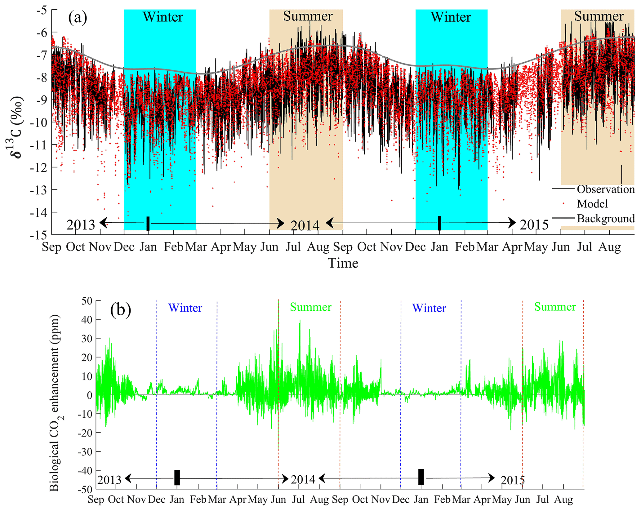
Figure 7(a) Comparisons of observed and modeled hourly δ13C-CO2 from September 2013 to August 2015, where the grey line represents derived δ13C-CO2 background, and (b) simulated hourly biological CO2 enhancement. The shade and lines in both subfigures represent the periods for winter and summer, respectively.

Figure 8Comparisons of observed and modeled (a) CO2 mixing ratio and (b) δ13C-CO2 from December 2013 to February 2014, (c) CO2 mixing ratio and (b) δ13C-CO2 from December 2014 to February 2015, (e) CO2 mixing ratio and (f) δ13C-CO2 from June to August 2014, and (g) CO2 mixing ratio and (h) δ13C-CO2 from June to August 2015.
Table 2Statistical metrics between observed and modeled CO2 mixing ratios and δ13C-CO2 during winter, summer, and annual for 2014 and 2015. Correlation coefficient (R), averages, and root mean square error (RMSE) are displayed.
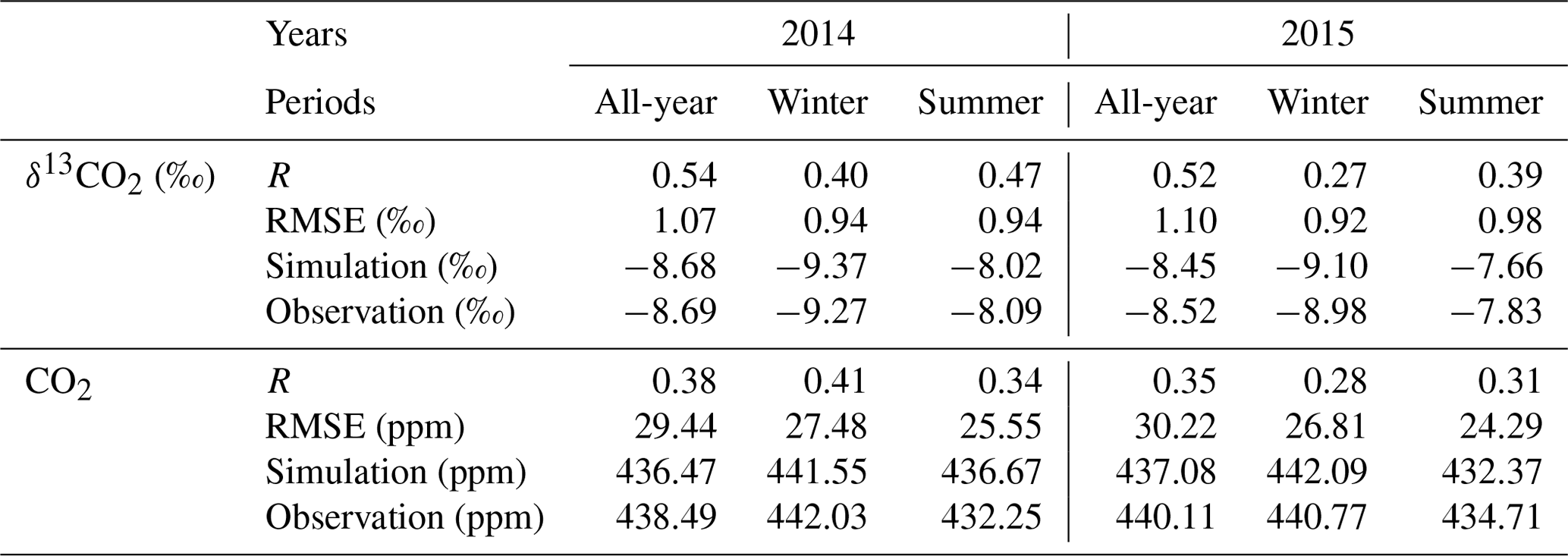
Here, we examine the comparisons for winter and summer in greater detail. The simulations showed that the model can generally capture the diel variations of observed hourly δ13C-CO2 variations (Fig. 8). Statistics between observations and simulations for the two seasons are shown in Table 2. The observed seasonal average increased substantially, by 1.18 ‰, from winter 2013–2014 (−9.27 ‰) to summer 2014 (−8.09 ‰). The simulations showed a similar seasonal increase of 1.35 ‰. Some large discrepancies are evident and generally caused by the simulated total CO2 enhancement biases (potentially caused by poorly simulated PBLH during these periods) and the negative relationship between δ13C-CO2 and the CO2 enhancement as shown in Fig. S6.
Comparisons between observations and simulations for the daily average CO2 mixing ratio and δ13C-CO2 are also shown in Fig. 9. Although the data are distributed around the 1 : 1 line for both seasons, there is less scatter and higher correlation in the winter than in the summer. We attributed this to the more complex biological CO2 sinks in the summer, which are not adequately resolved by the relatively coarse model grid (1∘ by 1∘). We also performed comparisons by only choosing the daytime observations. The results indicated that daytime CO2 mixing ratio simulations in the summer were slightly underestimated. This caused δ13C-CO2 to be overestimated (Fig. S7). The simulations for winter generally captured the trends for both CO2 and δ13C-CO2 when the biological CO2 enhancement played a relatively small role compared to anthropogenic emissions. The larger bias in the summer could result from the relatively coarse spatial–temporal resolution (aggregation error) of the Carbon Tracker biological CO2 flux, which was 1∘ × 1∘ with a 3 h average. As shown in Fig. S3, the spatial distribution of land use is far more heterogeneous. This will smooth the stronger biological CO2 signals by averaging it over the large 1∘ × 1∘ grid, while the urban biological CO2 flux occurs at much finer spatial scales and likely varies at shorter time intervals.
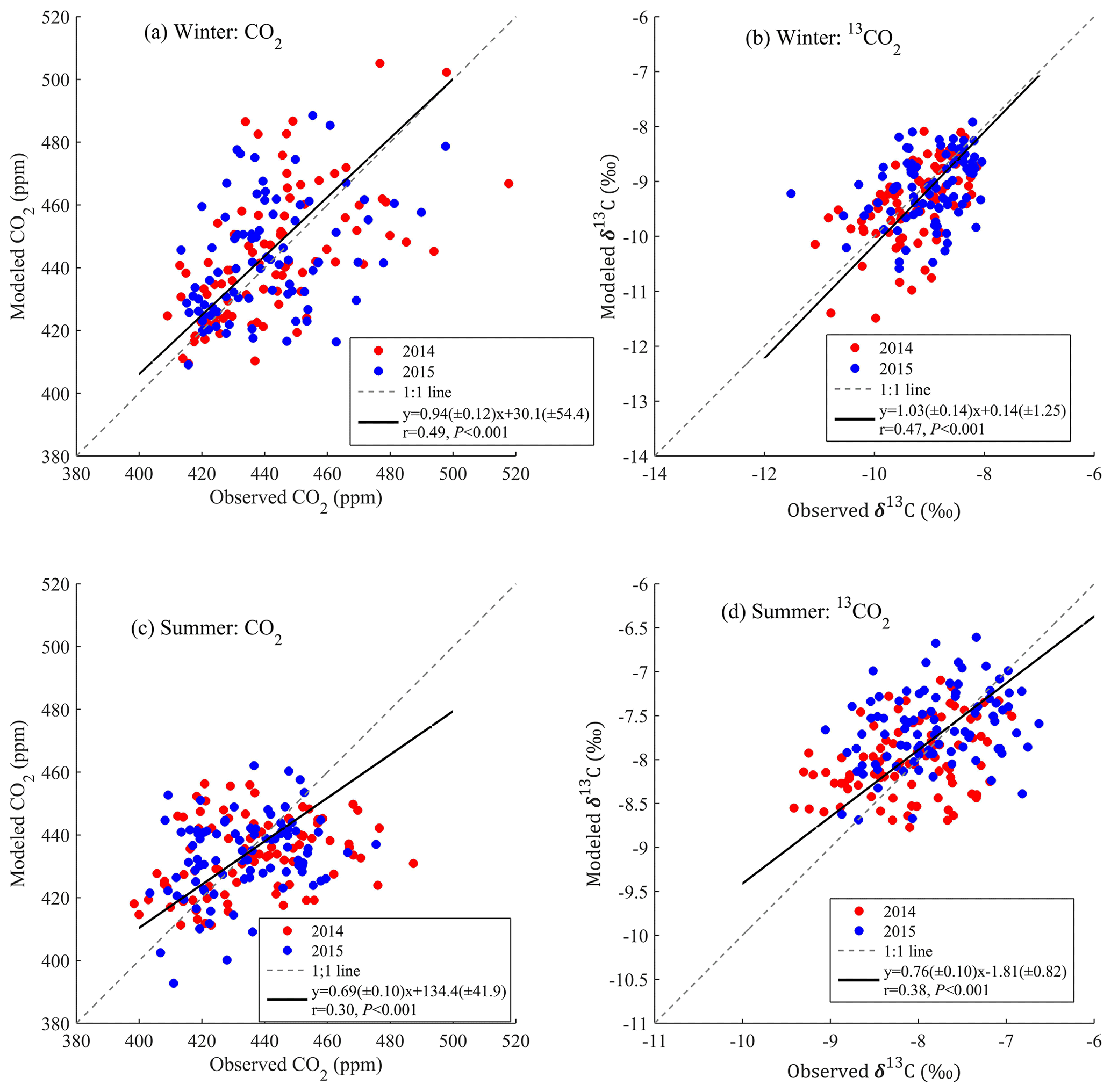
Figure 9Scatter plots of observed versus modeled (a) wintertime CO2 mixing ratios, (b) wintertime δ13C-CO2, (c) summertime CO2, and (d) summertime δ13C-CO2 for both years; here, these dots are daily averages.
3.2.3 Mechanisms controlling the δ13C-CO2 seasonality
The mechanisms driving these seasonal variations are examined below. The peak and trough in the observed δ13C-CO2 signal were observed in December and July (Fig. 10a), respectively, yielding an amplitude of 1.51 ‰. This was consistent with the simulated amplitude of 1.53 ‰. These results support the fact that the simulated δ13C-CO2 seasonality agreed well with the observations (Fig. 10) and can be used to further diagnose the mechanisms contributing to the δ13C-CO2 seasonality. According to Eq. (2), the δ13C-CO2 seasonality can be attributed to four factors, including (1) a change in the background δ13C-CO2 value from −7.64 ‰ in December to −6.66 ‰ in July, (2) a change in CO2 background from 399 to 398 ppm, (3) the total CO2 enhancement change from 45.7 to 37.3 ppm, and (4) the change in the isotope composition of the CO2 enhancements causing δs to vary from −26.1 ‰ to −22.8 ‰.
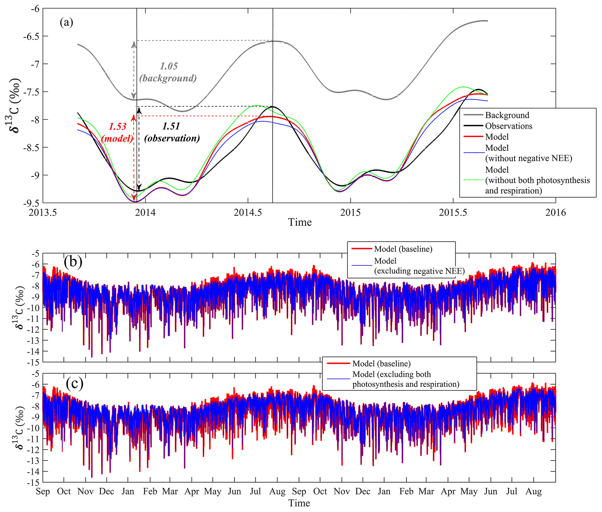
Figure 10Digital filtering curve fitting (CCGCRV) for background, observations, normal simulations, case 1 (excluding negative NEE when photosynthesis is stronger than respiration), and case 2 (excluding respiration and photosynthesis) in both years, (b) δ13C-CO2 comparisons between normal simulations and case 1, and (c) δ13C-CO2 comparisons between normal simulations and case 2.
To quantify each mechanism's contribution to the seasonality of atmospheric δ13C-CO2, we recalculated δ13C-CO2 by using the monthly averages as described above. First, we calculated δ13C-CO2 in December and July, which were −9.54 ‰ and −8.04 ‰, respectively, with an amplitude of 1.50 ‰. Next, we replaced the δ13C-CO2 background value in December (−7.64 ‰) with July (−6.67 ‰). The recalculated δ13C-CO2 was −8.66 ‰ in December, indicating that the change in δ13C-CO2 background value caused a change of 0.88 ‰ (9.54 ‰ minus −8.66 ‰) to the seasonality. By changing both the total CO2 enhancement and background values, the recalculated δ13C-CO2 was −8.32 ‰, contributing a 0.34 ‰ change in the seasonality (−8.66 ‰ minus −8.32 ‰). Finally, by changing δs from −26.1 ‰ to −22.8 ‰, together with the change in background value, the recalculated δ13C-CO2 was −8.32 ‰, a change of 0.34 ‰ (i.e., −8.66 ‰ minus −8.32 ‰). This indicates that both the total CO2 enhancement and change in δs contributed equally to the regional source term, causing a variation of 0.62 ‰ (i.e., 1.50 ‰ minus 0.88 ‰). Based on the above analyses, we attributed 59 % and 41 % of the δ13C-CO2 seasonality to the changing δ13C background term and regional source terms, respectively. Further, the total CO2 enhancement and change in δs, the sum of which can be treated as a regional source term, contributed equally (about 20 %) to the δ13C-CO2 seasonality.
To investigate how ecosystem photosynthetic discrimination and respiration affected atmospheric δ13C-CO2 seasonality, we simulated the δ13C-CO2 again for two cases: (1) excluding negative NEE when photosynthesis is stronger than respiration and (2) excluding both photosynthetic discrimination and respiration. Note that only NEE was used in our study, with no partitioning between photosynthesis and respiration in the daytime. The only role of photosynthetic discrimination should be stronger than in case 1, when only negative NEE is used. The results are shown in Fig. 10b–c. Overall, the negative CO2 enhancement caused atmospheric δ13C-CO2 to become more enriched in the baseline simulations, with maximum values around 1 ‰ between April and October (Fig. 10b), and positive CO2 enhancement (i.e., via net respiration) caused atmospheric δ13C-CO2 to become more depleted compared to the baseline simulations through the whole year (Fig. 10c). By applying the CCGRCV fitting technique to the δ13C-CO2 for the above two cases, we found that the δ13C-CO2 seasonality decreased to 1.45 ‰ in case 1, indicating ecosystem photosynthetic discrimination explained >0.08 ‰ of the seasonality (1.53 ‰ minus 1.45 ‰). For case 2, the δ13C-CO2 trough in winter slightly increased by 0.08 ‰, and the peak in summer increased by 0.20 ‰; these two factors finally led the seasonality to increase to 1.66 ‰, which was caused by much larger respiration CO2 enhancement in summer than in winter (Fig. 7b). These results indicate that biological respiration reduced the δ13C-CO2 seasonality by 0.20 ‰ and that negative NEE (photosynthetic discrimination) acted to increase the δ13C-CO2 seasonality by 0.08 ‰. Generally, both ecosystem photosynthesis and respiration played minor roles in controlling the atmospheric δ13C-CO2 seasonality within this urban area. In other words, the anthropogenic CO2 emissions played a much larger role than the plants.
As shown in Fig. 5, CO2 sources from the power industry, combustion for manufacturing, non-metallic mineral production and oil refineries and the transformation industry were the top four contributors to the CO2 enhancements. We simulated atmospheric δ13C-CO2 by assuming that no CO2 was emitted from each of these four categories. The simulations were performed by excluding one category at a time. The results indicated that atmospheric δ13C-CO2 seasonality was 1.30 ‰, 1.57 ‰, 1.30 ‰, and 1.47 ‰ when excluding the power industry, combustion for the manufacturing source, oil refineries/transformation industry, and non-metallic mineral production sources, respectively. In other words, the power industry and oil refineries/transformation industry together contributed 0.40 ‰ to the total regional source term of 0.62 ‰. The cement sources played a role in enriching by 0.07 ‰ the atmospheric δ13C-CO2 in the heavy isotope, contrary to all other anthropogenic CO2 sources.
3.3 Sensitivity analysis
3.3.1 Comparison of δs ⋅ ΔCO2
Based on Eq. (2), the regional source term determines the hourly/daily variations of δ13C-CO2, which is treated as a signal added to the background signal. To evaluate the model-simulated regional source term with respect to the observations, we examined daily averages for winter to minimize the influence of photosynthesis. In Fig. 11a, the observed daily δs ⋅ ΔCO2 values are compared with the simulated values using the a priori anthropogenic CO2 emissions. Here ΔCO2 represents the total CO2 enhancement for both observations and simulations. The product δs ⋅ ΔCO2 can be interpreted as the regional source term. The average values were −1009.0 (and −841.9) ppm ‰ for observations and −1096.7 (and 1000.5) ppm ‰ for model results in 2014 (and 2015). The slope of the regression fit was 0.99 (± 0.12), and the intercept was −151.7 (± 130.1) for all data during the two winters. After applying the monthly scaling factors to constrain the anthropogenic CO2 emissions, the re-calculated results were closer to the 1 : 1 line with a slightly improved correlation (R increased from 0.47 to 0.50; Fig. 11b). Note that the application of the monthly scaling factors only impacts the ΔCO2 but not δs. The uncertainty in δs will be discussed next.
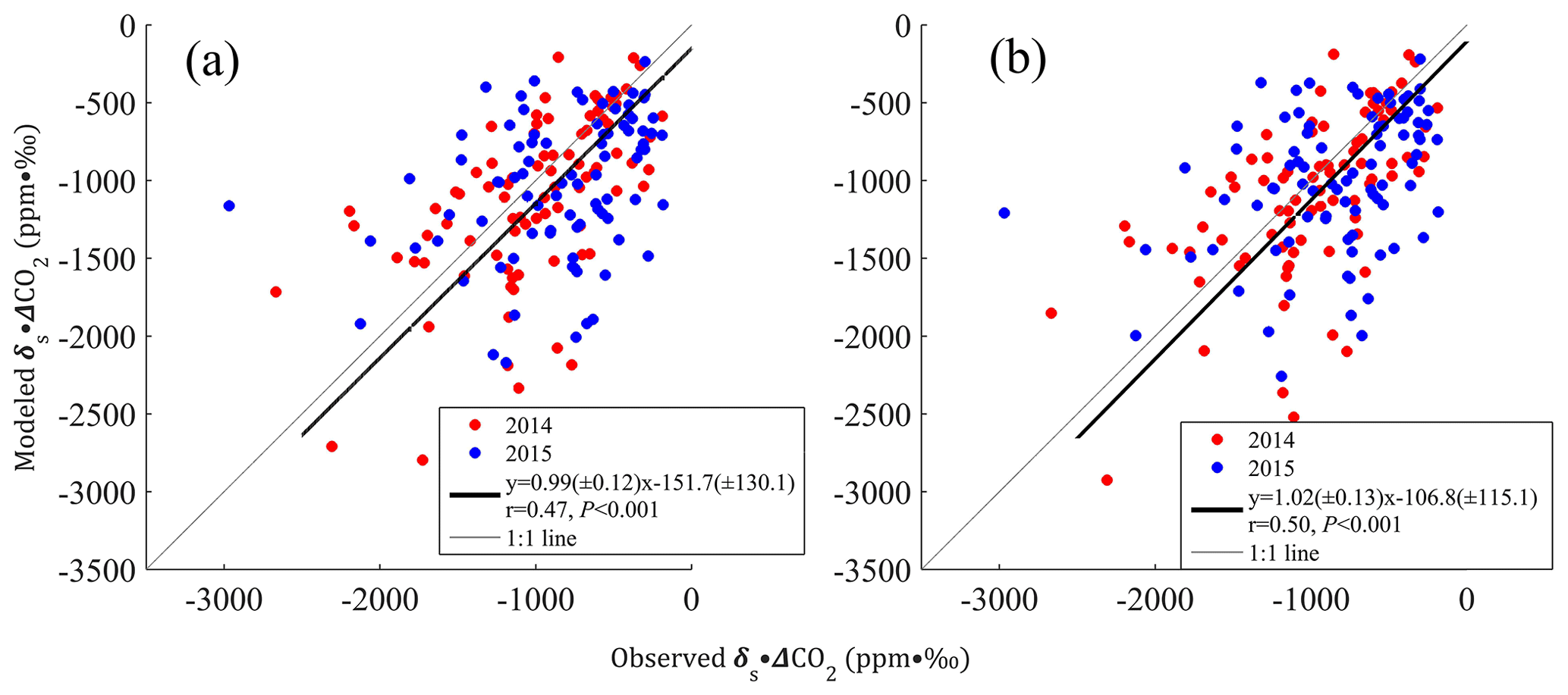
Figure 11Comparisons of wintertime δs ⋅ ΔCO2 using (a) a priori and (b) constrained anthropogenic CO2 emissions.
3.3.2 Comparison between δs_sim and δs
To evaluate the δs simulations, we compared observed and simulated δs as displayed in Fig. 12a for all-day and nighttime conditions. Here, nighttime simulations were selected to minimize the effects of ecosystem photosynthesis and to mainly focus on the anthropogenic CO2 sources. Two methods were used to calculate δs from the observations, including the Miller–Tans and Keeling plot methods. Although δs differed between these two methods, both displayed similar seasonal variations, with higher values (δ13C enrichment) in summer and lower values in winter. Such seasonal variations were also observed at other urban sites, including Beijing, China (Pang et al., 2016), Bern, Switzerland (Sturm et al., 2006), Bangalore, India (Guha and Ghosh, 2010), and Wroclaw, Poland (Górka and Lewicka-szczebak, 2013).

Figure 12(a) Comparisons between observed and modeled δs, (b) relationship between cement CO2 enhancement proportion and simulated anthropogenic δs for nighttime, and (c) all-day.
If the CO2 sources/sinks are homogeneously distributed and without monthly variations, the atmospheric CO2 enhancement components would remain unchanged, and there would be no seasonal changes in δs. In reality, variations in atmospheric transport processes interact with regional CO2 sink/source changes that cause monthly variations in δs. The comparison of δs between simulations and observations indicated that the model performed well in capturing the mixing and transport of CO2 from different sources. We can also infer from their difference that the proportions of some CO2 categories were biased in the a priori emission map. This can be caused by both the downscaling of EDGAR inventory distribution to 0.1∘ and the magnitude of some emissions categories. Among all anthropogenic sources, the most significant linear relations were found between the simulated anthropogenic δs and cement CO2 proportions for these 24 months, with slopes of 0.33 ‰ for nighttime and 0.35 ‰ for all-day conditions (R2=0.97, p<0.001; Fig. 12b and c). These results also indicated that cement CO2 emissions dominated monthly δs variations in the YRD region.
3.3.3 Sensitivity of atmospheric δ13C-CO2 and δs to cement CO2 emissions
The discrepancy between simulated and observed δs highlights that some CO2 sources were biased in the a priori inventories. As discussed above, cement CO2 emissions had the most distinct δ13C-CO2 end-member value of 0 ‰ ± 0.30 ‰ when compared with the averages of other anthropogenic sources. Combined with its large emission compared to other regions of the world, it had a strong potential to influence δs and δ13C-CO2. YRD represents the largest cement-producing region in the world (USGS, 2014; Cai et al., 2015; Yang et al., 2017). Its relative proportion to total national anthropogenic CO2 emissions is about 5.5 % to 6.5 % based on the IPCC method and 7.3 % for EDGAR. These proportions are 50 % greater than the global average of 4 % (Boden et al., 2016) and much larger than most countries (Andrew, 2018) and other large urbanized areas such as California (2 %; Cui et al., 2019).

Figure 13Sensitivity tests showing the influence of cement CO2 emissions on δs for (a) nighttime, (b) all-day, and (c) the relation between cement CO2 and δ13C for simulation strategies 1 (there is no bias in the total anthropogenic CO2 enhancement such that a proportional increase/decrease in the cement component does not change the relative anthropogenic contributions) and 2 (only the cement enhancement changes). Note that the numbers in brackets indicate changes in δ13C with cement CO2 enhancement proportion (the fraction of cement CO2 enhancement to simulated total CO2 enhancement) increase by 0.2 times. The x-axis values indicate changing cement enhancement proportions to 0.8, 1.2, 1.4, 1.6, 1.8, and 2 times the original values.
The local activity data reveal that the cement production increased from 3.55×10⁸ t in 2010 to 4.56×10⁸ t in 2014 in the YRD area. Our own calculation of the national clinker-to-cement ratio indicated a decreasing trend from 64 % in 2004 to around 56 % in 2015. Here, we applied the value of 61.7 % for 2010 and the average value of 57.0 % for 2014 to 2015. We then used the EF for clinker (0.52 ± 0.01 t CO2 per tonne clinker; IPCC, 2019). Finally, the calculated cement CO2 emissions were 1.14 (± 0.02) × 108 t for 2010 and 1.35 (± 0.03) × 108 t for 2014, indicating an 18.4 % increase over this time period. This result is close to the scaling factor of 1.145 for the total anthropogenic CO2 emissions for the same period.
The cement CO2 emission was 1.45 × 10⁸ t for the EDGAR products in 2010. Applying the scaling factor of 1.184, based on our independent method, the EDGAR cement CO2 emission was 1.72 × 10⁸ t for the year of 2014. The 27 % difference between the EDGAR inventory and our independent calculations probably resulted from large errors in the clinker-to-cement ratio and regional activity data. Ke et al. (2013) reported a much higher clinker-to-cement ratio of 73 % to 70 % for China during 2005 and 2007 than the ratio of 57 % in 2014 to 2015. If we applied a 70 % ratio, the EDGAR cement CO2 emission would change to 1.28 × 10⁸ t for 2010.
The monthly cement emission proportions varied from 6.21 % to 8.98 %, while its enhancement proportion was much larger and could reach 16.85 %. In other words, favorable atmospheric transport processes amplified the cement CO2 enhancement proportion at our observational site (Table S2). To quantify the extent to which the cement CO2 enhancement components can affect δs and atmospheric δ13C-CO2, we conducted sensitivity tests by changing the cement enhancement proportions to 0.8, 1.2, 1.4, 1.6, 1.8, and 2 times its original value. These sensitivity tests are based on two different assumptions for cement CO2 enhancement changes. (1) There is no bias in the total anthropogenic CO2 enhancement such that a proportional increase/decrease in the cement component does not change the relative anthropogenic contributions. (2) Only the cement enhancement changes. From Eq. (2), these two assumptions will change both δs and δ13C-CO2 but with different amplitude.
Results for the first assumption are shown in Fig. 13a–b for both nighttime and all-day δs simulations. The simulated δs increased linearly with the increase in cement proportions, at a rate of 2.73 ‰ increase per 10 % increase in cement proportions in the nighttime and 2.72 ‰ for all-day. The result for the second assumption is similar to the first one, yielding a 2.32 ‰ increase for a 10 % increase in the cement proportion. As shown in Table S2, the cement CO2 enhancement proportions increased from 5.60 %–6.77 % (December) to 13.16 %–16.85 % (June), which is the primary cause of the observed monthly δs variations. The high sensitivity of δs to cement CO2 proportions can partly explain the relative difference of modeled δs and indicates a potential advantage to constrain cement CO2 emissions by using atmospheric δ13C-CO2 observations. Finally we calculated how cement CO2 can change atmospheric δ13C-CO2 (Fig. 13c). These results show that atmospheric δ13C-CO2 is more sensitive to the first assumption than the second assumption. These sensitivity analyses indicate that a cement CO2 enhancement relative change of 20 % (or absolute 1.57 % increase) can cause a 0.013 ‰–0.038 ‰ change in the atmospheric δ13C-CO2. These results indicate that δs is sensitive to cement CO2 emissions.
Total annual anthropogenic CO2 emissions for the YRD showed a high consistency between the top-down and bottom-up approaches, with a bias of less than 6 %.
Approximately 59 % and 41 % of the δ13C-CO2 seasonality were attributed to the change in δ13C background value and the regional CO2 source term, respectively.
The power industry and oil refinery/transformation industry together contributed 0.40 ‰ to the seasonal cycle, accounting for 64.5 % in all regional source terms (0.62 ‰).
When excluding all ecosystem respiration and photosynthetic discrimination in the YRD area, δ13C-CO2 seasonality will increase from 1.53 ‰ to 1.66 ‰.
Atmospheric transport processes in summer amplified the cement CO2 enhancement proportions in the YRD area, which dominated monthly δs variations. δs calculated from simulations was shown to have a strong linear relationship with the cement CO2 EDGAR v4.3.2 inventory proportion in the YRD area.
The data presented in this paper have been uploaded on our group website: https://yncenter.sites.yale.edu/data-access (Xu and Lee, 2018).
The supplement related to this article is available online at: https://doi.org/10.5194/acp-21-10015-2021-supplement.
CH, TJG and XL designed the study, and CH performed the model simulation and wrote the original draft. Supervision was by TJG and XL. Data acquisition was by JX, WH, DY, YC, CL, SL, and LD. All the co-authors contributed to the data analysis.
The authors declare that they have no conflict of interest.
Publisher's note: Copernicus Publications remains neutral with regard to jurisdictional claims in published maps and institutional affiliations.
We thank Yale-NUIST group members who contributed to the long time atmospheric carbon dioxide mixing ratio and its carbon isotope observations. Cheng Hu also thanks Matt Erickson, Julian Deventer, Xiang Li, Ke Xiao, Zicong Chen, Xueying Yu and Xin Chen for weekly group meeting of model running and tall tower GHG observations in UMN. We also want to express our thanks to editor Manvendra K. Dubey and two anonymous referees: they provided insightful suggestions for improving this paper.
This work is supported by the National Key R&D Program of China (grant nos. 2020YFA0607501 and 2019YFA0607202), and Cheng Hu was supported by the Natural Science Foundation of Jiangsu Province (grant no. BK20200802); this work is also supported by the National Natural Science Foundation of China (grant no. 42021004), Natural Science Foundation of Jiangsu Province (grant no. BK20181100), and Key Research Foundation of the Jiangsu Meteorological Society (grant no. KZ201803).
This paper was edited by Manvendra K. Dubey and reviewed by two anonymous referees.
Alden, C. B., Miller, J. B., and Gatti, L. V.: Regional atmospheric CO2 inversion reveals seasonal and geographic differences in Amazon net biome exchange, Glob. Change Biol., 22, 3427–3443, https://doi.org/10.1111/gcb.13305, 2016.
Andrew, R. M.: Global CO2 emissions from cement production, Earth Syst. Sci. Data, 10, 195–217, https://doi.org/10.5194/essd-10-195-2018, 2018.
Ballantyne, A. P., Miller, J. B., Baker, I. T., Tans, P. P., and White, J. W. C.: Novel applications of carbon isotopes in atmospheric CO2: what can atmospheric measurements teach us about processes in the biosphere?, Biogeosciences, 8, 3093–3106, https://doi.org/10.5194/bg-8-3093-2011, 2011.
Berezin, E. V., Konovalov, I. B., Ciais, P., Richter, A., Tao, S., Janssens-Maenhout, G., Beekmann, M., and Schulze, E.-D.: Multiannual changes of CO2 emissions in China: indirect estimates derived from satellite measurements of tropospheric NO2 columns, Atmos. Chem. Phys., 13, 9415–9438, https://doi.org/10.5194/acp-13-9415-2013, 2013.
Boden, T., Andres, R., and Marland, G.: Global, Regional, and National Fossil-Fuel CO2 Emissions (1751–2013) (V. 2016), Environmental System Science Data Infrastructure for a Virtual Ecosystem; Carbon Dioxide Information Analysis Center (CDIAC), Oak Ridge National Laboratory (ORNL) [Data set], Oak Ridge, TN, USA, 2016.
Bréon, F. M., Broquet, G., Puygrenier, V., Chevallier, F., Xueref-Remy, I., Ramonet, M., Dieudonné, E., Lopez, M., Schmidt, M., Perrussel, O., and Ciais, P.: An attempt at estimating Paris area CO2 emissions from atmospheric concentration measurements, Atmos. Chem. Phys., 15, 1707–1724, https://doi.org/10.5194/acp-15-1707-2015, 2015.
Brioude, J., Angevine, W. M., Ahmadov, R., Kim, S.-W., Evan, S., McKeen, S. A., Hsie, E.-Y., Frost, G. J., Neuman, J. A., Pollack, I. B., Peischl, J., Ryerson, T. B., Holloway, J., Brown, S. S., Nowak, J. B., Roberts, J. M., Wofsy, S. C., Santoni, G. W., Oda, T., and Trainer, M.: Top-down estimate of surface flux in the Los Angeles Basin using a mesoscale inverse modeling technique: assessing anthropogenic emissions of CO, NOx and CO2 and their impacts, Atmos. Chem. Phys., 13, 3661–3677, https://doi.org/10.5194/acp-13-3661-2013, 2013.
Cai, B., Wang, J., He, J., and Geng, Y.: Evaluating CO2 emission performance in China's cement industry: An enterprise perspective, Appl. Energ., 166, 191–200, https://doi.org/10.1016/j.apenergy.2015.11.006, 2015.
Cao, C., Lee, X., Liu, S., Schultz, N., Xiao, W., Zhang, M., and Zhao, L.: Urban heat islands in China enhanced by haze pollution, Nat. Commun., 7, 12509, https://doi.org/10.1038/ncomms12509, 2016.
Chen, B., Chen, J., Tans, P., and Huang, L.: Simulating dynamics of δ13C of CO2 in the planetary boundary layer over a boreal forest region: covariation between surface fluxes and atmospheric mixing, Tellus, 58, 537–549, https://doi.org/10.1111/j.1600-0889.2006.00213.x, 2006.
Chen, J. M., Mo, G., and Deng, F.: A joint global carbon inversion system using both CO2 and 13CO2 atmospheric concentration data, Geosci. Model Dev., 10, 1131–1156, https://doi.org/10.5194/gmd-10-1131-2017, 2017.
Cui, X., Newman, S., Xu, X., Andrews, A. E., Miller, J., and Lehman, S.: Atmospheric observation-based estimation of fossil fuel CO2 emissions from regions of central and southern California, Sci. Total Environ., 664, 381–391, https://doi.org/10.1016/j.scitotenv.2019.01.081, 2019.
Deng, L., Liu, S., and Zhao, X.: Study on the change in land cover of Yangtze River Delta based on MOD13A2 data, China Science Paper, 10, 1822–1827, 2015 (in Chinese).
Gately, C. K. and Hutyra, L. R.: Large uncertainties in urban-scale carbon emissions, J. Geophys. Res.-Atmos., 122, 11242–11260, https://doi.org/10.1002/2017JD027359, 2017.
Gately, C. K., Hutyra, L. R., and Wing, I. S.: Cities, traffic, and CO2: A multidecadal assessment of trends, drivers, and scaling relationships, P. Natl. Acad. Sci. USA, 112, 4999–5004, https://doi.org/10.1073/pnas.1421723112, 2015.
Ghasemifard, H., Vogel, F. R., Yuan, Y., Luepke, M., Chen, J., Ries, L., Leuchner, M., Schunk, C., Noreen Vardag, S., and Menzel, A.: Pollution Events at the High-Altitude Mountain Site Zugspitze-Schneefernerhaus (2670 m a.s.l.), Germany, Atmosphere, 10, 330, https://doi.org/10.3390/atmos10060330, 2019.
Graven, H. D., Fischer, M. L., Lueker, T., Jeong, S., Guilderson, T. P., and Keeling, R.: Assessing fossil fuel CO2 emissions in California using atmospheric observations and models, Environ. Res. Lett., 13, 065007, https://doi.org/10.1088/1748-9326/aabd43, 2018.
Griffis, T. J.: Tracing the flow of carbon dioxide and water vapor between the biosphere and atmosphere: A review of optical isotope techniques and their application, Agr. Forest Meteorol., 174–175, 85–109, 2013.
Griffis, T. J., Sargent, S., Baker, J., Lee, X., Tanner, B., Greene, J., Swiatek, E., and Billmark, K.: Direct measurement of biosphere-atmosphere isotopic CO2 exchange using the eddy covariance technique, J. Geophys. Res.-Atmos., 113, D08304, https://doi.org/10.1029/2007JD009297, 2008.
Górka, M. and Lewicka-Szczebak, D.: One-year spatial and temporal monitoring of concentration and carbon isotopic composition of atmospheric CO2 in a Wroclaw (SW Poland) city area, Appl. Geochem., 35, 7–13, https://doi.org/10.1016/j.apgeochem.2013.05.010, 2013.
Guha, T. and Ghosh, P.: Diurnal variation of atmospheric CO2 concentration and δ13C in an urban atmosphere during winter-role of the Nocturnal Boundary Layer, J. Atmos. Chem., 65, 1–12, https://doi.org/10.1007/s10874-010-9178-6, 2010.
He, J., Naik, V., Horowitz, L. W., Dlugokencky, E., and Thoning, K.: Investigation of the global methane budget over 1980–2017 using GFDL-AM4.1, Atmos. Chem. Phys., 20, 805–827, https://doi.org/10.5194/acp-20-805-2020, 2020.
Hu, C., Liu, S., Wang, Y., Zhang, M., Xiao, W., Wang, W., and Xu, J.: Anthropogenic CO2 emissions from a megacity in the Yangtze River Delta of China, Environ. Sci. Pollut. R., 25, 23157–23169, https://doi.org/10.1007/s11356-018-2325-3, 2018a.
Hu, C., Griffis, T. J., Lee, X., Millet, D. B., Chen, Z., Baker, J. M., and Xiao, K.: Top-Down constraints on anthropogenic CO2 emissions within an agricultural-urban landscape, J. Geophys. Res.-Atmos., 123, 4674–4694, https://doi.org/10.1029/2017JD027881, 2018b.
Hu, C., Griffis, T. J., Liu, S., Xiao, W., Hu, N., Huang, W., Yang D., and Lee X.: Anthropogenic methane emission and its partitioning for the Yangtze River Delta region of China, J. Geophys. Res.-Biogeo., 124, 1148–1170, https://doi.org/10.1029/2018JG004850, 2019.
Hu, L., Andrews, A. E., Thoning, K. W., Sweeney, C., Miller, J. B., and Michalak, A. M.: Enhanced North American carbon uptake associated with El Niño, Sci. Adv., 5, eaaw0076, https://doi.org/10.1126/sciadv.aaw0076, 2019.
IEA: CO2 Emissions from Fuel Combustion 1971–2010, 2012 Edn., International Energy Agency (IEA), Paris, 2012.
IPCC (Intergovernmental Panel on Climate Change): 2019 Refinement to the 2006 IPCC Guidelines for National Greenhouse Gas Inventories, available at: https://www.ipcc-nggip.iges.or.jp/ public/2019rf/ (last access: 24 April 2021), 2019.
Janssens-Maenhout, G., Crippa, M., Guizzardi, D., Muntean, M., Schaaf, E., Dentener, F., Bergamaschi, P., Pagliari, V., Olivier, J. G. J., Peters, J. A. H. W., van Aardenne, J. A., Monni, S., Doering, U., and Petrescu, A. M. R.: EDGAR v4.3.2 Global Atlas of the three major Greenhouse Gas Emissions for the period 1970–2012, Earth Syst. Sci. Data Discuss. [preprint], https://doi.org/10.5194/essd-2017-79, 2017.
Jiang, F., Wang, H. M., Chen, J. M., Machida, T., Zhou, L. X., Ju, W. M., Matsueda, H., and Sawa, Y.: Carbon balance of China constrained by CONTRAIL aircraft CO2 measurements, Atmos. Chem. Phys., 14, 10133–10144, https://doi.org/10.5194/acp-14-10133-2014, 2014.
Ke, J., Mcneil, M., Price, L., and Zhou, N.: Estimation of CO2 emissions from China's cement production: Methodologies and uncertainties, Energy Policy, 57, 172–181, https://doi.org/10.1016/j.enpol.2013.01.028, 2013.
Keeling, C. D.: The concentration and isotopic abundances of carbon dioxide in the atmosphere, Tellus, 12, 200–203, https://doi.org/10.1111/j.2153-3490.1960.tb01300.x, 1960.
Lai, C., Ehleringer, J. R., Tans, P., and Wofsy, S. C.: Estimating photosynthetic 13C discrimination in terrestrial CO2 exchange from canopy to regional scales, Global Biogeochem. Cy., 18, GB1041, https://doi.org/10.1029/2003gb002148, 2014.
Lauvaux, T., Miles, N. L., Deng, A., Richardson, S. J., Cambaliza, M. O., Davis, K. J., and Wu, K.: High-resolution atmospheric inversion of urban CO2 emissions during the dormant season of the Indianapolis flux experiment (INFLUX), J. Geophys. Res.-Atmos., 121, 5213–5236, https://doi.org/10.1002/2015JD024473, 2016.
Li, X. and Xiao, J.: A global, 0.05-degree product of solar-induced chlorophyll fluorescence derived from OCO-2, MODIS, and reanalysis data, Remote Sens., 11, 517, https://doi.org/10.3390/rs11050517, 2019.
Martin, C. R., Zeng, N., Karion, A., Mueller, K., Ghosh, S., and Lopez-coto, I.: Investigating sources of variability and error in simulations of carbon dioxide in an urban region, Atmos. Environ., 199, 55–69, https://doi.org/10.1016/j.atmosenv.2018.11.013, 2019.
McManus, J. B., Nelson, D. D., and Zahniser, M. S.: Long-term continuous sampling of 12CO2, 13CO2 and 12C18O16O in ambient air with a quantum cascade laser spectrometer, Isot. Environ. Healt. S., 46, 49–63, https://doi.org/10.1080/10256011003661326, 2010.
Miller, J. B., Tans, P. P., White, J. W. C., Conway, T. J., and Vaughn, B. W.: The atmospheric signal of terrestrial carbon isotopic discrimination and its implication for partitioning carbon fluxes, Tellus B, 55, 197–206, https://doi.org/10.1034/j.1600-0889.2003.00019.x, 2003.
Miller, J. B., Lehman, S. J., Verhulst, K. R., Miller, C. E., Duren, R. M., Yadav, V., Newman, S., and Sloop, C. D.: Large and seasonally varying biospheric CO2 fluxes in the Los Angeles megacity revealed by atmospheric radiocarbon, P. Natl. Acad. Sci. USA, 117, 26681–26687, https://doi.org/10.1073/pnas.2005253117, 2020.
Moore, J. and Jacobson, A. D.: Seasonally varying contributions to urban CO2 in the Chicago, Illinois, USA region: Insights from a high-resolution CO2 concentration and δ13C record, Elementa, 3, 000052, https://doi.org/10.12952/journal.elementa.000052, 2015.
Mueller, K., Yadav, V., Lopez-Coto, I., Karion, A., Gourdji, S., Martin, C., and Whetstone, J.: Siting Background Towers to Characterize Incoming Air for Urban Greenhouse Gas Estimation: A Case Study in the Washington, DC/Baltimore Area, J. Geophys. Res.-Atmos., 123, 2910–2926, https://doi.org/10.1002/2017JD027364, 2018.
Nathan, B., Lauvaux, T., Turnbull, J. C., and Richardson, S.: Source Sector Attribution of CO2 Emissions Using an Urban CO/CO2 Bayesian Inversion System, J. Geophys. Res.-Atmos., 123, 13611–13621, https://doi.org/10.1029/2018JD029231, 2018.
Newman, S., Xu, X., Affek, H. P., Stolper, E., and Epstein S.: Changes in mixing ratio and isotopic composition of CO2 in urban air from the Los Angeles basin, California, between 1972 and 2003, J. Geophys. Res., 113, D23304, https://doi.org/10.1029/2008JD009999, 2008.
Newman, S., Xu, X., Gurney, K. R., Hsu, Y. K., Li, K. F., Jiang, X., Keeling, R., Feng, S., O'Keefe, D., Patarasuk, R., Wong, K. W., Rao, P., Fischer, M. L., and Yung, Y. L.: Toward consistency between trends in bottom-up CO2 emissions and top-down atmospheric measurements in the Los Angeles megacity, Atmos. Chem. Phys., 16, 3843–3863, https://doi.org/10.5194/acp-16-3843-2016, 2016.
Oda, T., Maksyutov, S., and Andres, R. J.: The Open-source Data Inventory for Anthropogenic CO2, version 2016 (ODIAC2016): a global monthly fossil fuel CO2 gridded emissions data product for tracer transport simulations and surface flux inversions, Earth Syst. Sci. Data, 10, 87–107, https://doi.org/10.5194/essd-10-87-2018, 2018.
Pang, J., Wen, X., and Sun, X.: Mixing ratio and carbon isotopic composition investigation of atmospheric CO2 in Beijing, China, Sci. Total Environ., 539, 322–330, https://doi.org/10.1016/j.scitotenv.2015.08.130, 2016.
Pataki, D. E., Bowling, D. R., Ehleringer, J. R., and Zobitz, J. M.: High resolution atmospheric monitoring of urban carbon dioxide sources, Geophys. Res. Lett., 33, L03813, https://doi.org/10.1029/2005GL024822, 2006.
Peters, W., Jacobson, A. R., Sweeney, C., Andrews, A. E., Conway, T. J., Masarie, K., John, B. M., Lori, M. P. B., Gabrielle, P., Adam, I. H., Douglas, E. J. W., Guido, R. v., James, T. R., Paul, O. W., Maarten, C. K., and Pieter, P. T.: An atmospheric perspective on North American carbon dioxide exchange: CarbonTracker, P. Natl. Acad. Sci. USA, 104, 18925–18930, https://doi.org/10.1073/pnas.0708986104, 2007.
Pillai, D., Buchwitz, M., Gerbig, C., Koch, T., Reuter, M., Bovensmann, H., Marshall, J., and Burrows, J. P.: Tracking city CO2 emissions from space using a high-resolution inverse modelling approach: a case study for Berlin, Germany, Atmos. Chem. Phys., 16, 9591–9610, https://doi.org/10.5194/acp-16-9591-2016, 2016.
Prairie, Y. T. and Duarte, C. M.: Direct and indirect metabolic CO2 release by humanity, Biogeosciences, 4, 215–217, https://doi.org/10.5194/bg-4-215-2007, 2007.
Rayner, P. J., Raupach, M. R., Paget, M., Peylin, P., and Koffi, E.: A new global gridded data set of CO2 emissions from fossil fuel combustion: Methodology and evaluation, J. Geophys. Res.-Atmos., 115, D19306, https://doi.org/10.1029/2009JD013439, 2010.
Ribeiro, H. V., Rybski, D., and Kropp, J. P.: Effects of changing population or density on urban carbon dioxide emissions, Nat. Commun., 10, 3204, https://doi.org/10.1038/s41467-019-11184-y, 2019.
Ruckstuhl, A. F., Henne, S., Reimann, S., Steinbacher, M., Vollmer, M. K., O'Doherty, S., Buchmann, B., and Hueglin, C.: Robust extraction of baseline signal of atmospheric trace species using local regression, Atmos. Meas. Tech., 5, 2613–2624, https://doi.org/10.5194/amt-5-2613-2012, 2012.
Sargent, M., Barrera, Y., Nehrkorn, T., Hutyra, L. R., Gately, C. K., Mckain, K., Sweeney, C., Hegarty, J., Hardiman, B., Steven, C., and Wofsy, S. C.: Anthropogenic and biogenic CO2 fluxes in the Boston urban region, P. Natl. Acad. Sci. USA, 115, 7491–7496, https://doi.org/10.1073/pnas.1803715115, 2018.
Schneising, O., Heymann, J., Buchwitz, M., Reuter, M., Bovensmann, H., and Burrows, J. P.: Anthropogenic carbon dioxide source areas observed from space: assessment of regional enhancements and trends, Atmos. Chem. Phys., 13, 2445–2454, https://doi.org/10.5194/acp-13-2445-2013, 2013.
Seto, K. C., Dhakal, S., Bigio, A., Blanco, H., Delgado, G. C., and Dewar, D.: Human settlements, infrastructure, and spatial planning, in: Climate change 2014: Mitigation ofclimate change, Contribution of working group III to the fifth assessment report of the intergovernmental panel on climate change, 923–1000, Cambridge University Press, Cambridge, UK and New York, NY, USA, https://doi.org/10.1017/CBO9781107415416.018, 2014.
Shen, S., Yang, D., Xiao, W., Liu, S., and Lee, X.: Constraining anthropogenic CH emissions in Nanjing and the Yangtze River Delta, China, using atmospheric CO and CH mixing ratios, Adv. Atmos. Sci., 31, 1343–1352, https://doi.org/10.1007/s00376-014-3231-3, 2014.
State Statistical Bureau: China Statistical Yearbook 2015, China Statistical Press, Beijing, China, 2016 (in Chinese).
Staufer, J., Broquet, G., Bréon, F.-M., Puygrenier, V., Chevallier, F., Xueref-Rémy, I., Dieudonné, E., Lopez, M., Schmidt, M., Ramonet, M., Perrussel, O., Lac, C., Wu, L., and Ciais, P.: The first 1-year-long estimate of the Paris region fossil fuel CO2 emissions based on atmospheric inversion, Atmos. Chem. Phys., 16, 14703–14726, https://doi.org/10.5194/acp-16-14703-2016, 2016.
Sturm, P., Leuenberger, M., Valentino, F. L., Lehmann, B., and Ihly, B.: Measurements of CO2, its stable isotopes, , and 222Rn at Bern, Switzerland, Atmos. Chem. Phys., 6, 1991–2004, https://doi.org/10.5194/acp-6-1991-2006, 2006.
Sturm, P., Tuzson, B., Henne, S., and Emmenegger, L.: Tracking isotopic signatures of CO2 at the high altitude site Jungfraujoch with laser spectroscopy: analytical improvements and representative results, Atmos. Meas. Tech., 6, 1659–1671, https://doi.org/10.5194/amt-6-1659-2013, 2013.
Super, I., Denier van der Gon, H. A. C., van der Molen, M. K., Sterk, H. A. M., Hensen, A., and Peters, W.: A multi-model approach to monitor emissions of CO2 and CO from an urban–industrial complex, Atmos. Chem. Phys., 17, 13297–13316, https://doi.org/10.5194/acp-17-13297-2017, 2017.
Thompson, R. L., Patra, P. K., Chevallier, F., Maksyutov, S., Law, R. M., Ziehn, T., and Ciais, P.: Top-down assessment of the Asian carbon budget since the mid 1990s, Nat. Commun., 7, 1–10, https://doi.org/10.1038/ncomms10724, 2016.
Thoning, K. W., Tans, P. P., and Komhyr, W. D.: Atmospheric carbon dioxide at Mauna Loa observatory 2. Analysis of the NOAA/GMCC data, 1974–1985, J. Geophys. Res.-Atmos., 94, 8549–8565, https://doi.org/10.1029/JD094iD06p08549, 1989.
Turnbull, J. C., Sweeney, C., Karion, A., Newberger, T., Lehman, S. J., Tans, P. P., and Davis, K.: Toward quantification and source sector identification of fossil fuel CO2 emissions from an urban area: results from the influx experiment, J. Geophys. Res.-Atmos., 120, 292–312, https://doi.org/10.1002/2014JD022555, 2015.
Turner, A. J., Shusterman, A. A., McDonald, B. C., Teige, V., Harley, R. A., and Cohen, R. C.: Network design for quantifying urban CO2 emissions: assessing trade-offs between precision and network density, Atmos. Chem. Phys., 16, 13465–13475, https://doi.org/10.5194/acp-16-13465-2016, 2016.
USGS (U. S. Geological Survey): Mineral Commodity Summaries 2013, available at: http://minerals.usgs.gov/minerals/pubs/commodity/cement/ (last access: 6 August 2019), 2014.
Vardag, S. N., Gerbig, C., Janssens-Maenhout, G., and Levin, I.: Estimation of continuous anthropogenic CO2: model-based evaluation of CO2, CO, δ13C(CO2) and Δ14C(CO2) tracer methods, Atmos. Chem. Phys., 15, 12705–12729, https://doi.org/10.5194/acp-15-12705-2015, 2015.
Verhulst, K. R., Karion, A., Kim, J., Salameh, P. K., Keeling, R. F., Newman, S., Miller, J., Sloop, C., Pongetti, T., Rao, P., Wong, C., Hopkins, F. M., Yadav, V., Weiss, R. F., Duren, R. M., and Miller, C. E.: Carbon dioxide and methane measurements from the Los Angeles Megacity Carbon Project – Part 1: calibration, urban enhancements, and uncertainty estimates, Atmos. Chem. Phys., 17, 8313–8341, https://doi.org/10.5194/acp-17-8313-2017, 2017.
Wang, Y., Munger, J. W., Xu, S., McElroy, M. B., Hao, J., Nielsen, C. P., and Ma, H.: CO2 and its correlation with CO at a rural site near Beijing: implications for combustion efficiency in China, Atmos. Chem. Phys., 10, 8881–8897, https://doi.org/10.5194/acp-10-8881-2010, 2010.
Worden, H. M., Cheng, Y., Pfister, G., Carmichael, G. R., Zhang, Q., and Streets, D. G.: Satellite-based estimates of reduced CO and CO2 emissions due to traffic restrictions during the 2008 Beijing Olympics, Geophys. Res. Lett., 39, 1–6, https://doi.org/10.1029/2012GL052395, 2012.
Xu, J. and Lee, X.: Carbon dioxide concentration and 13C measurement in Nanjing (2013–2015), available at: https://yncenter.sites.yale.edu/data-access, last access: 1 August 2018.
Xu, J., Lee, X., Xiao, W., Cao, C., Liu, S., Wen, X., Xu, J., Zhang, Z., and Zhao, J.: Interpreting the 13C 12C ratio of carbon dioxide in an urban airshed in the Yangtze River Delta, China, Atmos. Chem. Phys., 17, 3385–3399, https://doi.org/10.5194/acp-17-3385-2017, 2017.
Yang, Y., Wang, L., Cao, Z. Mou C., Shen, L., Zhao, J., and Fang, Y.: CO2 emissions from cement industry in China: A bottom-up estimation from factory to regional and national levels, J. Geogr. Sci., 27, 711–730, 2017.
Zhang, H. F., Chen, B. Z., van der Laan-Luijkx, I. T., Chen, J., Xu, G., Yan, J. W., Zhou, L. X., Fukuyama, Y., Tans, P. P., and Peters, W.: Net terrestrial CO2 exchange over China during 2001–2010 estimated with an ensemble data assimilation system for atmospheric CO2, J. Geophys. Res.-Atmos., 119, 3500–3515, https://doi.org/10.1002/2013JD021297, 2014.
Zhao, C., Andrews, A. E., Bianco, L., Eluszkiewicz, J., Hirsh, A., Macdonald, C., Nehrkorn, T., and Fischer, M. L.: Atmospheric inverse estimates of methane emissions from Central California, J. Geophys. Res.-Atmos., 114, 4723–4734, https://doi.org/10.1029/2008JD011671, 2009.