An inversion of NO_x and non-methane volatile organic compound (NMVOC) emissions using satellite observations during the KORUS-AQ campaign and implications for surface ozone over East Asia

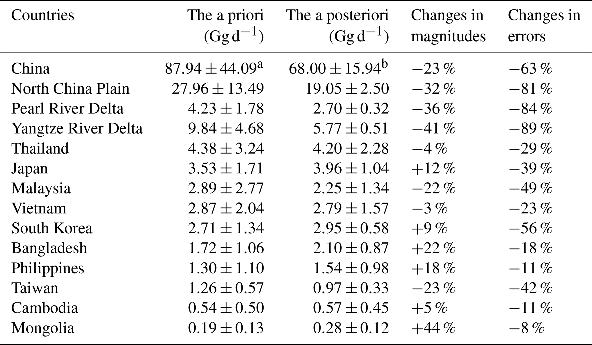
The absence of up-to-date emissions has been a major impediment to accurately simulating aspects of atmospheric chemistry and to precisely quantifying the impact of changes in emissions on air pollution. Hence, a nonlinear joint analytical inversion (Gauss–Newton method) of both volatile organic compounds (VOCs) and nitrogen oxide (NO_x) emissions is made by exploiting the Smithsonian Astrophysical Observatory (SAO) Ozone Mapping and Profiler Suite Nadir Mapper (OMPS-NM) formaldehyde (HCHO) and the National Aeronautics and Space Administration (NASA) Ozone Monitoring Instrument (OMI) tropospheric nitrogen dioxide (NO₂) columns during the Korea–United States Air Quality (KORUS-AQ) campaign over East Asia in May–June 2016. Effects of the chemical feedback of NO_x and VOCs on both NO₂ and HCHO are implicitly included by iteratively optimizing the inversion. Emission uncertainties are greatly narrowed (averaging kernels > 0.8, which is the mathematical presentation of the partition of information gained from the satellite observations with respect to the prior knowledge) over medium- to high-emitting areas such as cities and dense vegetation. The prior amount of total NO_x emissions is mainly dictated by values reported in the MIX-Asia 2010 inventory. After the inversion we conclude that there is a decline in emissions (before, after, change) for China (87.94±44.09 Gg d⁻¹, 68.00±15.94 Gg d⁻¹, −23 %), North China Plain (NCP) (27.96±13.49 Gg d⁻¹, 19.05±2.50 Gg d⁻¹, −32 %), Pearl River Delta (PRD) (4.23±1.78 Gg d⁻¹, 2.70±0.32 Gg d⁻¹, −36 %), Yangtze River Delta (YRD) (9.84±4.68 Gg d⁻¹, 5.77±0.51 Gg d⁻¹, −41 %), Taiwan (1.26±0.57 Gg d⁻¹, 0.97±0.33 Gg d⁻¹, −23 %), and Malaysia (2.89±2.77 Gg d⁻¹, 2.25±1.34 Gg d⁻¹, −22 %), all of which have effectively implemented various stringent regulations. In contrast, South Korea (2.71±1.34 Gg d⁻¹, 2.95±0.58 Gg d⁻¹, +9 %) and Japan (3.53±1.71 Gg d⁻¹, 3.96±1.04 Gg d⁻¹, +12 %) are experiencing an increase in NO_x emissions, potentially due to an increased number of diesel vehicles and new thermal power plants. We revisit the well-documented positive bias (by a factor of 2 to 3) of MEGAN v2.1 (Model of Emissions of Gases and Aerosols from Nature) in terms of biogenic VOC emissions in the tropics. The inversion, however, suggests a larger growth of VOCs (mainly anthropogenic) over NCP (25 %) than previously reported (6 %) relative to 2010. The spatial variation in both the magnitude and sign of NO_x and VOC emissions results in nonlinear responses of ozone production and loss. Due to a simultaneous decrease and increase in NO_x∕VOC over NCP and YRD, we observe a ∼53 % reduction in the ratio of the chemical loss of NO_x (LNO_x) to the chemical loss of RO_x (RO₂+HO₂) over the surface transitioning toward NO_x-sensitive regimes, which in turn reduces and increases the afternoon chemical loss and production of ozone through NO₂+OH (−0.42 ppbv h⁻¹)∕HO₂ (and RO₂)+NO (+0.31 ppbv h⁻¹). Conversely, a combined decrease in NO_x and VOC emissions in Taiwan, Malaysia, and southern China suppresses the formation of ozone. Simulations using the updated emissions indicate increases in maximum daily 8 h average (MDA8) surface ozone over China (0.62 ppbv), NCP (4.56 ppbv), and YRD (5.25 ppbv), suggesting that emission control strategies on VOCs should be prioritized to curb ozone production rates in these regions. Taiwan, Malaysia, and PRD stand out as regions undergoing lower MDA8 ozone levels resulting from the NO_x reductions occurring predominantly in NO_x-sensitive regimes.

1 Introduction

The study of ozone (O₃) formation within the troposphere in East Asia is of global importance. This significant pollutant is not confined to the source, as it spreads hemispherically through the air, affecting background concentrations as far away as the US. A study by Lin et al. (2017) provided modeling evidence of enhancements in springtime surface ozone levels (+0.5 ppbv yr⁻¹) in the western US in 1980–2014 solely due to the tripling of Asian anthropogenic emissions over the period. As more studies have provided information on the impact of ozone pollution on both human health and crop yields, Chinese governmental regulatory agencies have begun to take action on cutting the amount of NO_x (NO+NO₂) emissions since 2011–2012 (Gu et al., 2013; Reuter et al., 2014; Krotkov et al., 2016; de Foy et al., 2016; Souri et al., 2017a); however, no effective policy on volatile organic compound (VOC) emissions had been put into effect prior to 2016 (Stavrakou et al., 2017; Souri et al., 2017a; Shen et al., 2019; M. Li et al., 2019), with the exception of the Pearl River Delta (PRD) (Zhong et al., 2013). In addition to China, a number of governments including those of Malaysia and Taiwan have put a great deal of effort into shifting their energy pattern from consuming fossil fuels to renewable sources (Trappey el al., 2012; Chua and Oh, 2011). On the other hand, using satellite observations, Irie et al. (2016) and Souri et al. (2017a) revealed a systematic hiatus in the reduction of NO_x over South Korea and Japan, potentially due to increases in the number of diesel vehicles and new thermal power plants built to compensate for the collapse of the Fukushima nuclear power plant in 2011. Therefore, it is interesting to quantify to what extent these policies have impacted ozone pollution.

Unraveling the origin of ozone is complicated by a number of factors encompassing the nonlinearity of ozone formation to its sources, primarily from NO_x and VOCs. Therefore, to be able to quantify the impact of recent emission changes, we have developed a top-down estimate of relevant emission inventories using well-characterized satellite observations. There are a myriad of studies focusing on optimizing bottom-up anthropogenic and biogenic emissions using satellites observations, which provide high spatial coverage, in conjunction with chemical transport models for VOCs (e.g., Palmer et al., 2003; Shim et al., 2005; Curci et al., 2010; Stavrakou et al., 2009, 2011), and NO_x (e.g., Martin et al., 2003; Chai et al., 2009; Miyazaki et al., 2017; Souri et al., 2016a, 2017a, 2018). Most inverse modeling studies do not consider both NO₂ and formaldehyde (HCHO) satellite-based observations to perform a joint inversion. It has been shown that VOC and NO_x emissions can affect the production or loss of each other (Marais et al., 2012; Wolfe et al. 2016; Valin et al., 2016; Souri et al., 2020a). Consequently, a joint method that incorporates both species while minimizing the uncertainties in their emissions is better suited to address this problem. Dealing with this tangled relationship between VOC–NO₂ and NO_x–HCHO requires an iteratively nonlinear inversion framework to incrementally consider the relationships derived from a chemical transport model. Here we will provide an optimal estimate of NO_x and VOC emissions during the KORUS-AQ campaign using the Smithsonian Astrophysical Observatory (SAO) Ozone Mapping and Profiler Suite Nadir Mapper (OMPS-NM) HCHO and the National Aeronautics and Space Administration (NASA) Ozone Monitoring Instrument (OMI) NO₂ retrievals, whose accuracy and precisions are characterized against rich observations collected during the campaign. Having a top-down constraint on both emissions permits a more precise quantification of the impact of the recent emission changes on different chemical pathways pertaining to ozone formation and loss.

2 Measurements, modeling, and method

2.1 Remote sensing measurements

2.1.1 OMPS HCHO

OMPS-NM onboard the Suomi National Polar-orbiting Partnership (Suomi NPP) is a UV-backscattered radiation spectrometer launched in October 2011 (Flynn et al., 2014). Its revisit time is the same as other NASA A-Train satellites, including Aura at approximately 13:30 local time at the Equator in ascending mode. OMPS-NM covers 300–380 nm with a resolution of 1 nm full-width at half-maximum (FWHM). The sensor has a 340×740 pixel charge-coupled device (CCD) array measuring the UV spectra at a spatial resolution of 50×50 km² at nadir. The HCHO retrieval has been fully described in González Abad et al. (2015, 2016). Briefly, OMPS HCHO slant columns are fit using direct radiance fitting (Chance, 1998) in the spectral range 327.7–356.5 nm. The spectral fit requires a reference spectrum as a function of the cross-track position as it attempts to determine the number of molecules with respect to a reference (i.e., a differential spectrum fitting). To account for this, we use earthshine radiances over a relatively pristine area in the remote Pacific Ocean within −30 to +30 latitude. An upgrade to this reference correction is the use of daily HCHO profiles over monthly mean climatological ones from simulations done by the GEOS-Chem chemical transport model. On average, this leads to a 4 % difference in HCHO total columns with respect to using the monthly mean climatological values (Supplement Fig. S1). The scattering weights describing the sensitivity of the light path through a simulated atmosphere are calculated using VLIDORT (Spurr, 2006). The shape factors used for calculating air mass factors (AMFs) are derived from a regional chemical transport model (discussed later) that is used for carrying out the inversion in the present study. We remove unqualified pixels based on cloud fraction < 40 %, solar zenith angle < 65^∘, and a main quality flag provided in the data. We oversample the HCHO columns for the period of May–June 2016 using a Cressman spatial interpolator with a 1^∘ radius of influence.

2.1.2 OMI tropospheric NO₂

We use NASA OMI tropospheric NO₂ (version 3.1) level 2 data, whose retrieval is made in the violet–blue (402–465 nm) due to strong absorption of the molecule in this wavelength range (Levelt et al., 2018). The sensor has a nadir spatial resolution of 13×24 km², which can extend to 40×160 km² at the edge of scan lines. A more comprehensive description of the retrieval and the uncertainty associated with the data can be found in Krotkov et al. (2017) and Choi et al. (2020). We remove bad pixels based on cloud fraction < 20 %, solar zenith angle < 65^∘ (without the row anomaly), a vertical column density (VCD) quality flag of 0, and terrain reflectivity < 30 %. Similar to the OMPS HCHO, we recalculate AMFs by using shape factors from the chemical transport model used in this study. We oversample the OMI granules using the Cressman interpolator with a 0.25^∘ radius of influence.

Figure 1 The CMAQ 27 km domain covering the major proportion of Asia. The background picture is retrieved from the publicly available NASA Blue Marble (© NASA).

2.2 Model simulation

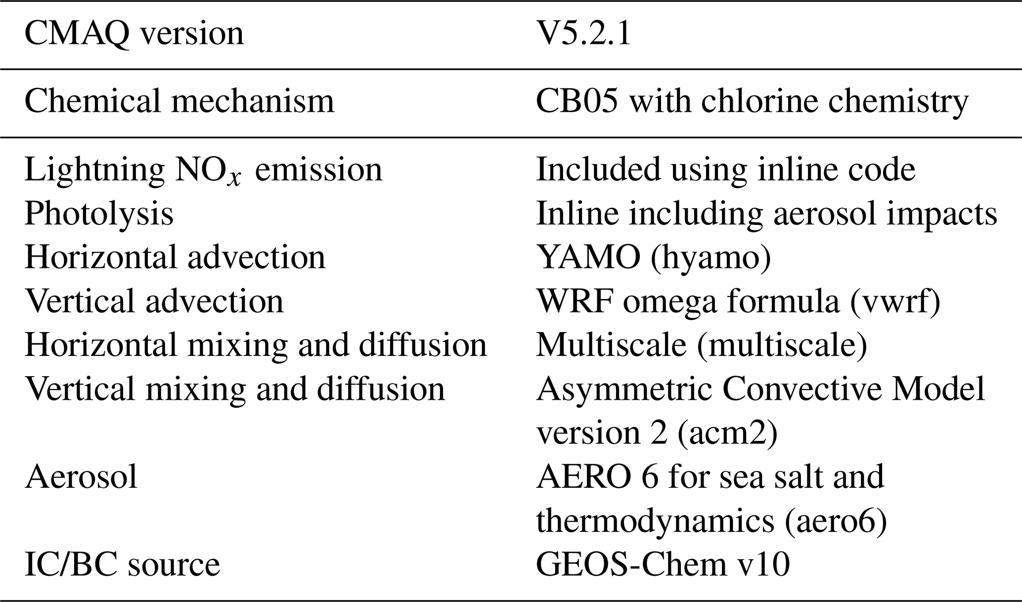
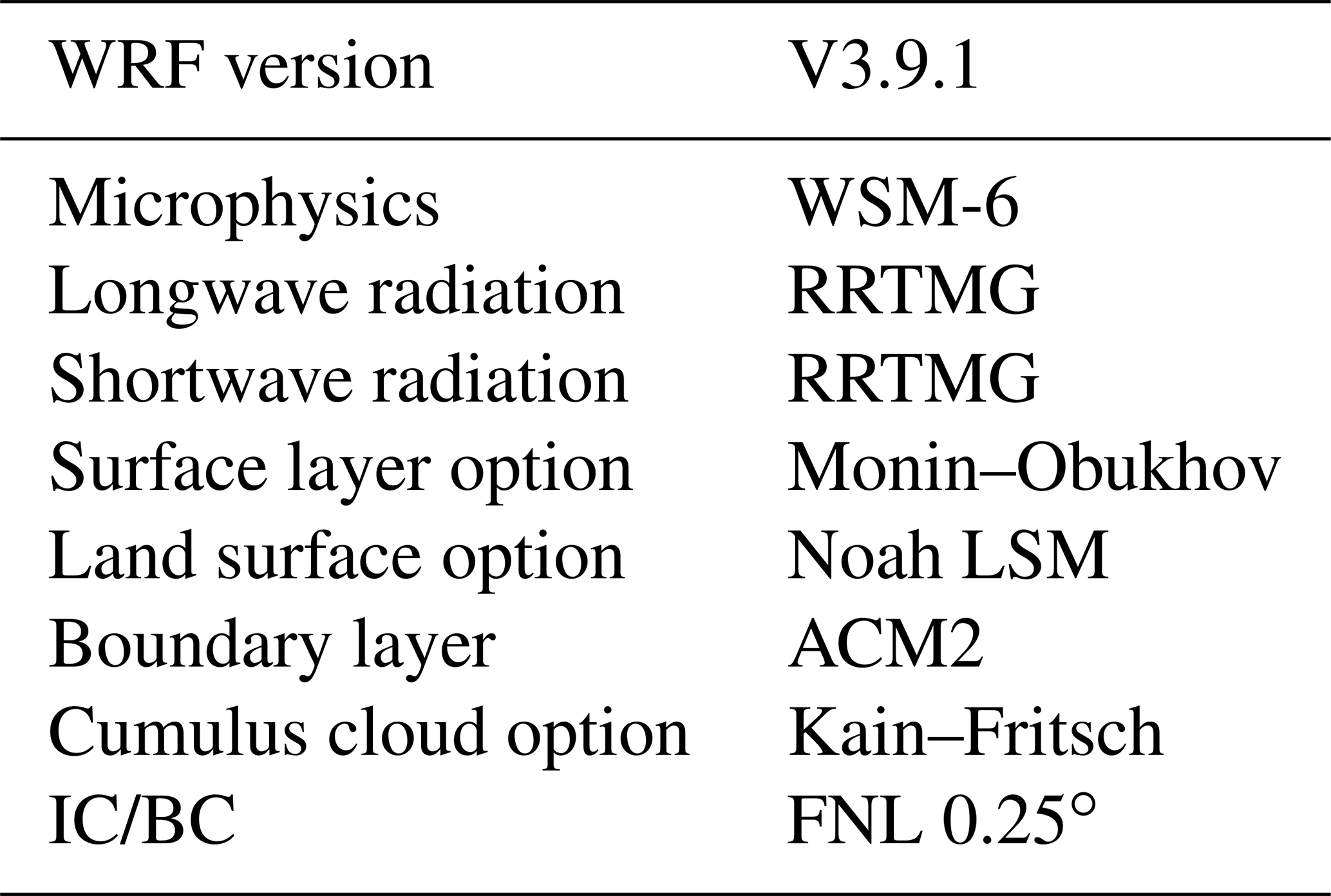
To be able to simulate the atmospheric composition, and to perform analytical inverse modeling, we set up a 27 km grid resolution regional chemical transport model using the Community Multiscale Air Quality Modeling System (CMAQ) model (v5.2.1; https://doi.org/10.5281/zenodo.1212601) (Byun and Schere, 2006) that consists of 328×323 grids covering China, Japan, South Korea, Taiwan, and some portions of Russia, India, and South Asia (Fig. 1). The time period covered by the simulation is from April to June 2016. We use the month of April for spin-up. The anthropogenic emissions are based on the monthly MIX-Asia 2010 inventory (Li et al., 2017) in the CB05 mechanism. The anthropogenic emissions are mainly grouped into three different sectors, namely mobile, point, and residential (area) sources. We apply a diurnal scale to the mobile sectors used in the National Emission Inventory (NEI) 2011 emission platform to represent the first-order approximation of traffic patterns. We include biomass burning emissions from the Fire Inventory from NCAR (FINN) v1.6 inventory (Wiedinmyer et al., 2011) and consider the plume rise parametrization used in the GEOS-Chem model (i.e., 60 % of emissions are distributed uniformly in the planetary boundary layer – PBL). We use the offline Model of Emissions of Gases and Aerosols from Nature (MEGAN) v2.1 model (Guenther et al., 2012) following the high-resolution inputs described in Souri et al. (2017). The diurnally varying lateral chemical conditions are simulated by GEOS-Chem v10 (Bey et al., 2001) using the full chemistry mechanism (NO_x–O_x–HC–Aer–Br) spun up for a year. With regard to weather modeling, we use the Weather Research and Forecasting (WRF) model v3.9.1 (Skamarock et al., 2008) at the same resolution as that of the CMAQ (∼27 km), but with a wider grid (342×337) and 28 vertical pressure sigma levels. The lateral boundary conditions and the grid nudging inputs are from the global Final (FNL) 0.25^∘ resolution model. The major configurations for the WRF-CMAQ model are summarized in Tables 1 and 2.

Table 1 CMAQ major configurations.

Table 2 WRF physics options.

2.3 Inverse modeling

We attempt to improve our high-dimensional imperfect numerical representation of atmospheric compounds using the well-characterized NO₂ and HCHO columns from satellites. We perform an analytical inversion using the WRF-CMAQ model to constrain the relevant bottom-up emission estimation (Souri et al., 2016a, 2017a, 2018). The inversion seeks to solve the following cost function under the assumptions that (i) both observation and emission error covariances follow Gaussian probability density functions with a zero bias, (ii) the observation and emission error covariances are independent, and (iii) the relationship between observations and emissions is not grossly nonlinear:

$$\begin{array}{}\text{(1)}& \begin{array}{rl}J\left(\mathit{x}\right)& ={\displaystyle \frac{\mathrm{1}}{\mathrm{2}}}{\left(\mathit{y}-F\left(\mathit{x}\right)\right)}^T{\mathbf{S}}_{\mathrm{o}}^{-\mathrm{1}}\left(\mathit{y}-F\left(\mathit{x}\right)\right)+{\displaystyle \frac{\mathrm{1}}{\mathrm{2}}}{\left(\mathit{x}-{\mathit{x}}_{\mathrm{a}}\right)}^T\\ & {\mathbf{S}}_{\mathrm{e}}^{-\mathrm{1}}\left(\mathit{x}-{\mathit{x}}_{\mathrm{a}}\right),\end{array}\end{array}$$

where x is the inversion estimate (a posteriori) given two sources of data, a priori (x_a) and observation (y). S_o and S_e are the error covariance matrices of the observation (instrument) and emission. F is the forward model (here WRF-CMAQ) to project the emissions onto columns. The first term of Eq. (1) attempts to reduce the distance between observations and the simulated columns. The second term incorporates some prior understanding and expectation of the true state of the emissions. The weight of each term is dictated by its covariance matrix. If S_e is large compared to S_o, the a posteriori will be independent of the prior knowledge and, conversely, if S_o dominates, the final solution will consist mostly of the a priori.

Following the Gauss–Newton method described in Rodgers (2000), we iteratively derive (i.e., i is the index of iteration) the posterior emissions by

$$\begin{array}{}\text{(2)}& {\mathit{x}}_{i+\mathrm{1}}=x_{\mathrm{a}}+\mathbf{G}\left[\mathit{y}-F\left({\mathit{x}}_i\right)+K_i\left({\mathit{x}}_i-{\mathit{x}}_{\mathrm{a}}\right)\right],\end{array}$$

where G is the Kalman gain,

$$\begin{array}{}\text{(3)}& \mathbf{G}={\mathbf{S}}_{\mathrm{e}}{K}_i^T{\left(K_i{\mathbf{S}}_{\mathrm{e}}{K}_i^T+{\mathbf{S}}_{\mathrm{o}}\right)}^{-\mathrm{1}},\end{array}$$

and K_i=K(x_i) is the Jacobian matrix calculated explicitly from the model (discussed later). The covariance matrix of the a posteriori is calculated by

$$\begin{array}{}\text{(4)}& {\widehat{\mathbf{S}}}_{\mathrm{e}}=\left(\mathbf{I}-\mathbf{G}{\widehat{K}}^T\right){\mathbf{S}}_{\mathrm{e}},\end{array}$$

where $\widehat{K}$is the Jacobian from the ith iteration. Here we iterate Eq. (2) three times. The averaging kernels (A) are given by

$$\begin{array}{}\text{(5)}& \mathbf{A}=\mathbf{I}-{\widehat{\mathbf{S}}}_{\mathrm{e}}{\mathbf{S}}_{\mathrm{e}}^{-\mathrm{1}}.\end{array}$$

The inversion system is complicated by the commonly overlooked fact that observations are biased. For instance, Souri et al. (2018) found that airborne remote sensing observations were high relative to surface Pandora measurements. The overestimation of the VCDs was problematic, since it could have been propagated in the inversion, inducing a bias in the top-down estimation. The authors partly mitigated it by constraining the MODIS albedo, which was assumed to be responsible for the bias. Attempts to reduce the bias resulting from coarse profiles from a global model in calculating gas shape profiles were made by recalculating the shape factors using those from higher-spatial-resolution regional models in other studies (e.g., Souri et al., 2016a; Laughner et al., 2018). For this study, we use abundant observations from the KORUS-AQ campaign and follow the intercomparison platform proposed by Zhu et al. (2016, 2020) using aircraft observations to be able to mitigate the biases in HCHO columns. Based on the corrected global model as a benchmark (Fig. S2), we scale up all OMPS HCHO columns by 20 %. To mitigate the potential biases in OMI NO₂, we exclusively followed the values reported over the KORUS-AQ period in Choi et al. (2020). We increase the NO₂ concentration uniformly by 33.9 % (see Table A3 in their paper).

We calculate the covariance matrix of observations using the column uncertainty variable provided in the satellite datasets and consider them to be random errors associated with spectrum fitting. We consider 25 % random errors for the air mass factors. Therefore, these values (as random errors) are significantly lowered by oversampling the data over the course of 2 months. In addition to that, we consider a fixed error for all pixels due to variability that exists in the applied bias correction (3.61×10¹⁵ molec. cm⁻² for NO₂ and 4.62×10¹⁵ molec. cm⁻² for HCHO). This error is based on the root mean square error (RMSE) obtained from the mentioned studies used for removing biases. Despite the fact that we do not account for non-diagonal elements of the covariance matrices, the incremental updates of G adjusted by both NO₂ and HCHO observations should better translate the covariance matrices into the emission space.

To increase the degree of freedom for the optimization, we combine all sector emissions including anthropogenic, biomass burning, and biogenic emissions for NO_x and VOCs. Therefore, we use the following formula to estimate the variance of the a priori:

$$\begin{array}{}\text{(6)}& {\mathit{\sigma }}_{\mathrm{total}}^{\mathrm{2}}=f_{\mathrm{anthro}}^{\mathrm{2}}\times {\mathit{\sigma }}_{\mathrm{anthro}}^{\mathrm{2}}+f_{\mathrm{BB}}^{\mathrm{2}}\times {\mathit{\sigma }}_{\mathrm{BB}}^{\mathrm{2}}+f_{\mathrm{bio}}^{\mathrm{2}}\times {\mathit{\sigma }}_{\mathrm{bio}}^{\mathrm{2}},\end{array}$$

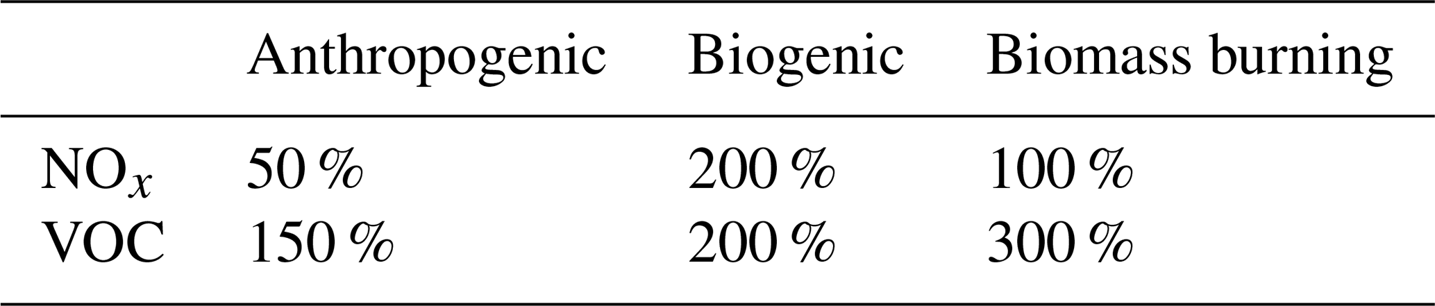
where f denotes the fraction of the emission sector with respect to the total emissions, and σ is the standard deviation of each sector category, which is calculated from the average of each sector to a relative error listed in Table 3.

Table 3 The uncertainty assumptions used for estimating the covariance matrix of the a priori.

For the same purpose (enhancing the amount of information gained from satellite observations) and to increase computational speed, we reduce the dimension of the state vectors (emissions) by aggregating them. However, grouping emissions into certain zones could also introduce another type of uncertainty, known as the aggregation error. We choose optimally aggregated zones by running the inversion multiple times, each with a certain selection of state vectors (Turner and Jacob, 2015). As in our previous study in Souri et al. (2018), we use the Gaussian model mixture (GMM) method to cluster emissions into certain zones that share roughly similar features and investigate which combinations will lead to a minimum of the sum of aggregation and smoothing errors.

In order to create the K matrix, one must estimate the impact of changes in emissions for each of the aggregated zones on the concentrations of a target compound, which is calculated using the CMAQ direct decoupled method (DDM) (Dunker et al., 1989; Cohan et al., 2005). For instance, the first row and column of K denoting the response of the first grid cell to a zonal emission can be obtained by

$$\begin{array}{}\text{(7)}& K_{\left(\mathrm{1},\mathrm{1}\right)}={\displaystyle \frac{S_{\left(\mathrm{1},\mathrm{1}\right)}^{{\mathrm{NO}}_{\mathrm{2}}}}{{\mathrm{ENO}}_x^{\mathrm{total},\mathrm{zone}}}},\end{array}$$

where $S_{\left(\mathrm{1},\mathrm{1}\right)}^{{\mathrm{NO}}_{\mathrm{2}}}$ is the DDM output in molecules per square centimeter (molec. cm⁻²) for the first row and column. It explains the resultant change in the NO₂ column by changing one unit of total NO_x emissions. The same concept will be applied to HCHO and VOC emissions. We do not consider the transport between zones due to computational burdens; therefore, we assume that the HCHO and NO₂ columns are mostly confined to their sources in the 2-month averages. The advantage of using CMAQ DDM to estimate the sensitivity lies in the fact that it calculates the local gradient, which better represents the nonlinear relationship between the emissions and the columns (Souri et al., 2017a, 2018); this, in turn, reduces the number of iterations.

3 Validation of the model in terms of meteorology

It is essential to first evaluate some key meteorological variables because large errors in the weather can complicate the inversion (e.g., Liu et al. 2017). In order to validate the performance of the WRF model in terms of a number of meteorological variables, including surface temperature, relative humidity, and winds, we use more than 1100 surface measurements from integrated surface database (ISD) stations (https://www.ncdc.noaa.gov/isd, last access: 12 September 2019) over the domain in May–June 2016. Table 4 lists the comparison of the model and the observations for the mentioned variables. Our model demonstrates a very low bias (0.6 ^∘C) with regard to surface temperature. We find a reasonable correspondence in terms of relative humidity, indicating a fair water vapor budget in the model. The largest discrepancy between the model and observations with respect to temperature and humidity occurs in grid cells that are in the proximity of the boundary conditions (not shown). Concerning the wind components, the deviation of the model from the observations is smaller than results obtained in a relatively flat area like Houston in Souri et al. (2016a, b).

Table 4 Statistics for surface temperature, relative humidity, and wind. Corr – correlation; RMSE – root mean square error; MAE – mean absolute error; MB – mean bias; O – observation; M – model; O_M – observed mean; M_M – model mean; SD – standard deviation. Units for RMSE, MAE, MB/O_M, M_M, O_SD, and M_SD: degrees Celsius for temperature, percentage for relative humidity, and meters per second for wind.

4 Comparison to satellites and providing top-down emissions

Prior to updating the emissions, we find it necessary to shed light on the spatial distribution of tropospheric NO₂ and HCHO columns from both observations and the model, as well as their potential differences relative to their key precursors' emissions. Subsequently, we report the results from the inverse modeling and the uncertainty associated with the top-down estimation; moreover, we wish to assess how much information is gained from utilizing satellite observations via the calculation of averaging kernels. Finally, observations are used to verify, to some extent, the accuracy of our top-down emission estimations.

4.1  NO_x

The first row in Fig. 2 illustrates tropospheric NO₂ columns from the regional model, OMI (using adjusted AMF and bias-corrected), and the natural logarithmic ratio of both quantities in May–June 2016 at ∼13:30 LST over Asia. The second row depicts daily mean values of dominant sources of NO_x, namely as biogenic, anthropogenic, and biomass burning emissions (that are subject to change after the inversion). A high degree of correlation between anthropogenic NO_x emissions and NO₂ columns implies the predominant production of NO₂ from the anthropogenic sources (Logan, 1983). We find a reasonable two-dimensional Pearson correlation (r=0.73) between the modeled and the observed columns. Generally, the WRF-CMAQ largely underestimated (56 %, $-\mathrm{7.72}\times {\mathrm{10}}^{\mathrm{14}}$ molec. cm⁻²) tropospheric NO₂ columns with respect to those of OMI over the entire domain. Intuitively segregating the domain into high-emission areas (NO_x > 10 t d⁻¹) and low ones (NO_x < 10 t d⁻¹) allows for a better understanding of the discrepancy between the model and the observations. In the high NO_x areas, the model tends to overestimate tropospheric NO₂ columns by 73 % (3.71×10¹⁵ molec. cm⁻²), whereas for the low NO_x regions, the model shows a substantial underestimation by 68 % ($-\mathrm{8.97}\times {\mathrm{10}}^{\mathrm{14}}$ molec. cm⁻²). Such a conflicting bias is confirmed by the contour map of the natural logarithm ratio of OMI to the model in Fig. 2. The large overestimation of the model in terms of NO₂ over polluted areas is explained by stringent regulations enacted in various countries in Asia; for instance, Chinese regulatory agencies have recently taken aggressive actions to cut anthropogenic NO_x emissions by implementing selective catalytic reductions in power plants, closing a number of coal power plants, and implementing policies on transportation (Zhang et al., 2012; Liu et al., 2016; Reuter et al., 2014; de Foy et al., 2016; Krotkov et al., 2016; Souri et al., 2017a). The highest positive bias in the model is observed over Shanxi Province in China, home to coal production, underscoring the effectiveness of the emission standards at controlling NO_x emissions. Likewise, we observe a positive bias in the model over major cities in Japan and South Korea, but the magnitude of the reduction over these cities is substantially smaller than what we observe in China.

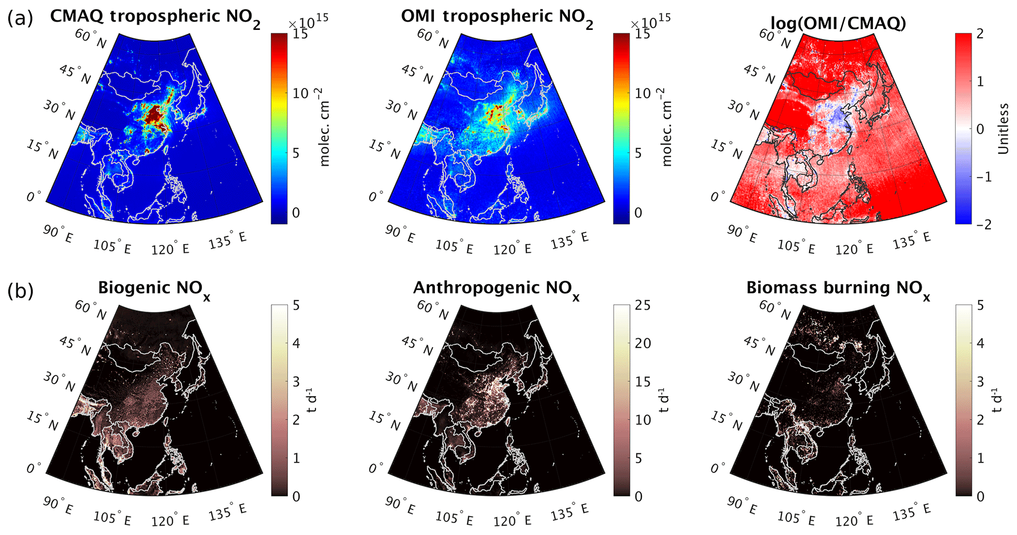
Figure 2 (a) Tropospheric NO₂ columns from the WRF-CMAQ model, OMI (using adjusted AMFs based on the shape factors derived from the model and bias-corrected following Choi et al., 2020), and the natural logarithmic ratio of OMI ∕ CMAQ during May–June 2016 at ∼13:30 LST. (b) The major sources of NO_x emissions in the region including biogenic (soil) emissions simulated by MEGAN, anthropogenic emissions estimated by MIX-Asia (2010), and biomass burning emissions made by FINN. The emissions are the daily mean values based on the emissions in May–June.

The underestimation of the model in the low NO_x regions is related to a number of factors, such as the following: (i) the widely reported underestimation of soil (biogenic) NO_x emissions due to a lack of precise knowledge of fertilizer use, soil biota, and/or canopy interactions (Jaeglé, et al., 2005; Hudman et al., 2010; Souri et al., 2016a); (ii) the underestimation of the upper-troposphere NO₂ due to non-surface emissions (aviation, lightning) or errors in the vertical mixing or moist convection (e.g., Souri et al., 2018); and (iii) a possible overprediction of the lifetime of organic nitrates diminishing background NO₂ levels (Canty et al., 2015). Addressing the second issue requires a very high-resolution model with explicit resolving microphysics and large eddy simulations, and the last problem requires more experimental studies to improve organic nitrate chemistry (Romer Present et al., 2020). In this study, we attempt to mitigate the discrepancy between the model and the satellite observations solely by adjusting the relevant emissions. Accordingly, future improvements in physical–chemical processes of models will inevitably offset top-down emission estimates.

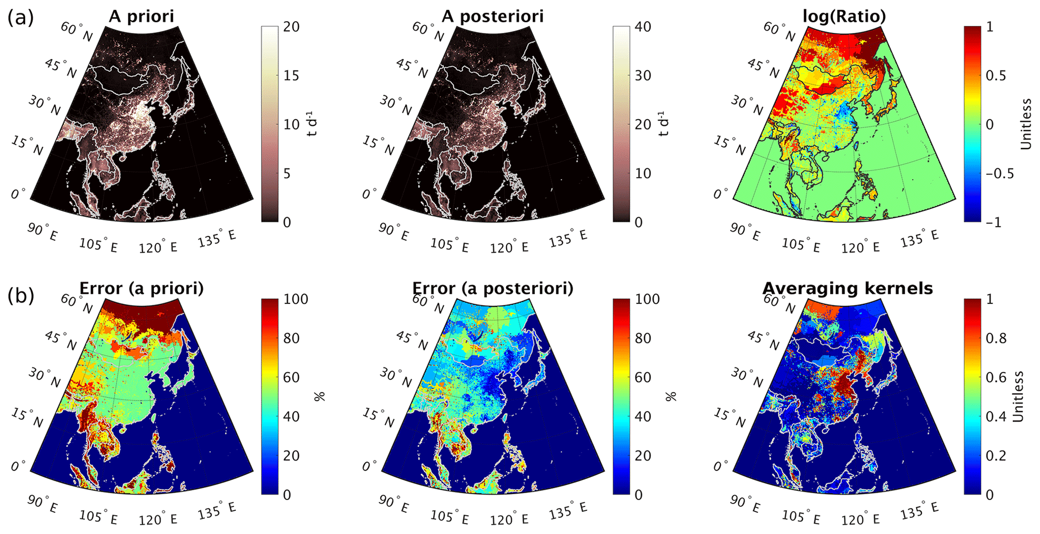
Figure 3 (a) Total NO_x emissions (i.e., the a priori) constrained by the satellite observations (i.e., the a posteriori) in May–June 2016 and the natural logarithmic ratio of the a posteriori to the a priori. (b) The errors in the a priori based on Table 3, the errors in the top-down estimation, and the averaging kernels (AKs) obtained from the estimation.

The first row in Fig. 3 shows the a priori, the a posteriori, and their ratios in terms of the total NO_x emissions in May–June 2016. We observe that the ratios are highly correlated with those of OMI ∕ CMAQ shown in Fig. 2, suggesting that the inversion attempts to reduce the distance between the model and the observations. Major reductions occur over China. The enhancements in NO_x emissions are commonly found in rural areas, especially over grasslands located in western–central China and Mongolia. The changes in NO_x emissions over South Korea and Japan are positive (Irie et al., 2016; Souri et al., 2017a), mainly due to rapid increases in the number of diesel cars in South Korea and thermal power plants built as a substitution for the Fukushima nuclear plant in Japan. This is especially the case for Japan for which we observe a larger enhancement in total NO_x emissions (12 %). The second row in Fig. 3 depicts the relative errors in the a priori, the a posteriori, and averaging kernels (AKs). Relative errors in the a priori are mostly confined to values close to 50 % in polluted areas. They increase further, up to 100 %, in areas experiencing relatively large contributions from biomass burning or biogenic (soil) emissions. Encouragingly, OMI tropospheric NO₂ columns in conjunction with the solid mathematical inversion method (Rodgers, 2000) greatly reduce the uncertainties associated with the emissions in polluted areas; we observe AKs close to 1 over major cities or industrial areas. We see the lowest values in AKs over rural areas due to weaker signal-to-noise ratios from the sensor. Therefore, it is desirable but very difficult to improve the model using the sensor with respect to NO_x chemistry and emissions in remote areas, evident in the low values of AKs. Table 5 lists the magnitude of the total NO_x emissions in several regions (refer to Fig. 1) before and after carrying out the inversion. If we assume that the dominant source of NO_x emissions is anthropogenic, the most successful countries at cutting emissions (before, after) are China (87.94±44.09 and 68.00±15.94 Gg d⁻¹), Taiwan (1.26±0.57 and 0.97±0.33 Gg d⁻¹), and Malaysia (2.89±2.77 and 2.25±1.34 Gg d⁻¹). All three countries have successfully implemented regulations to reduce anthropogenic emissions since 2010–2011 (Zhang et al., 2012; Trappey el al., 2012; Chua and Oh, 2011). The uncertainty associated with the top-down estimate improves considerably. The largest reduction in the uncertainty of the emissions is observed over China, a response to a strong signal from OMI.

Table 5 NO_x emissions before and after carrying out the inversion using OMI ∕ OMPS for different countries in May–June 2016.

^a The errors in the a priori are estimated from Eq. (6). ^b The errors in the a posteriori are calculated by Eq. (4).

An interesting observation lies in the discrepancy between the natural logarithm ratio of OMI ∕ CMAQ (Fig. 2) and that of the a posteriori to the a priori over the North China Plain (NCP), suggesting that using a bulk ratio (Martin et al., 2003) cannot fully account for possible chemical feedback. The natural logarithm ratio of OMI ∕ CMAQ is consistently lower than the changes in the emission. Two reasons contribute to this effect: (i) as NO_x emissions decrease in NO_x-saturated areas (i.e., the dominant sink of radicals is through NO₂+OH), OH levels essentially increase, resulting in a shorter lifetime of NO₂; therefore, to reduce NO₂ concentrations, a substantial reduction in NO_x (suggested by OMI ∕ CMAQ) is unnecessary, coinciding with results from the inverse modeling. Also, (ii) the CMAQ DDM (Fig. S3) suggests that NO₂ columns decrease due to increasing VOC emissions over the region; accordingly, the cross-relationship between NO₂ concentrations and VOC emissions partly adds to the discrepancy. It is because of the chemical feedback that recent studies have attempted to enhance the capability of inverse modeling by iteratively adjusting relevant emissions (e.g., Cooper et al., 2017; C. Li et al., 2019). Likewise, our iterative nonlinear inversion shows a superior performance over traditional bulk ratio methods, in part because it incrementally considers the chemical feedback.

To assess the resulting changes in the tropospheric NO₂ columns after the inversion, and to validate our results, we compare the simulated values using the a priori and the a posteriori with OMI in Fig. 4. We observe a 64 % reduction in the tropospheric NO₂ columns on average over NCP despite only a 32 % reduction in the total NO_x emissions over the region, a result of the chemical feedback. The two-dimensional Pearson correlation between the simulation using the a posteriori and OMI increases from 73 % (using the a priori) to 83 %. Both datasets now are in a better agreement as far as the magnitude goes. However, we do not see a significant change in the background values in the new simulation compared to those of OMI due to less certain column observations.

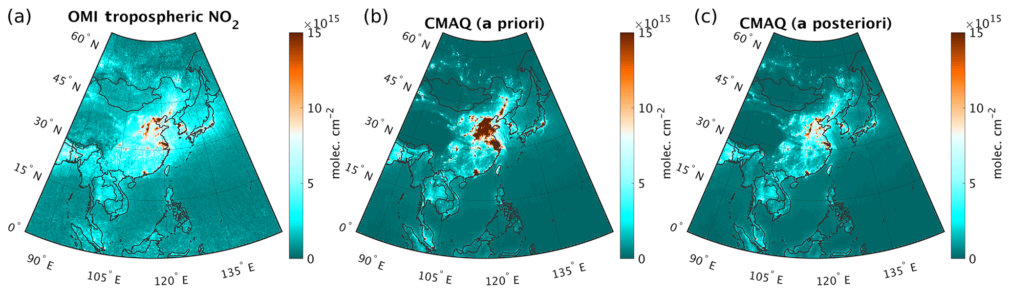
Figure 4 (a–c) Tropospheric NO₂ columns from OMI, WRF-CMAQ simulated with the prior emissions, and the same model but with the top-down emissions constrained by OMI ∕ OMPS in May–June 2016.

To further validate the results, we compare the NO₂ data from the NCAR four-channel chemiluminescence instrument onboard the DC-8 aircraft during the campaign (Fig. S4). These data are not interfered with by the NO_z family. The aircraft collected the data over the Korean Peninsula on around 23 d in May–June 2016, covering various altitudes and hours (https://www-air.larc.nasa.gov/cgi-bin/ArcView/korusaq, last access: 8 December 2019). We observe an underestimation of NO₂ at the near-surface levels (< 900 hPa) by 19 % (DC-8 =4.50 ppbv, CMAQ =3.67 ppbv). The updated emissions increase the near-surface levels over the Korean Peninsula, which in turn reduces the bias to 11 % (CMAQ =4.02 ppbv).

4.2 VOC

A comparison between HCHO columns from the model and OMPS along with the major sources of VOCs in May–June 2016 is depicted in Fig. 5. Anthropogenic VOCs are emitted from various sources such as solvent use and the mobile and chemical industries (Liu et al., 2008a, b). A reasonable correlation (r=0.78) between the model and OMPS suggests good confidence in the location of emissions. However, the magnitude of HCHO columns between the two datasets strongly disagrees, especially over the tropics where biogenic emissions are large. A myriad of studies have reported a largely positive bias (by a factor of 2–3) associated with isoprene emissions estimated by MEGAN using satellite measurements over the tropics (e.g., Millet et al., 2008; Stavrakou et al., 2009; Marais et al., 2012; Bauwens et al., 2016). To compound, Stavrakou et al. (2011) found a large overestimation in methanol emissions from the same model that can further preclude the accurate estimation of the yield of HCHO. As a response to the overestimation of the biogenic VOCs by MEGAN, we observe a largely positive bias in the simulated HCHO columns ranging from 50 % over the south of China to ∼400 % over Malaysia and Indonesia. As we move away from the hotspot of the biogenic emissions in lower latitudes, the positive bias of the model declines, ultimately turning into a negative bias at higher latitudes. OMPS HCHO columns suggest that the concentration of HCHO over NCP and Yangtze River Delta (YRD) is comparable to those over the tropics, suggesting that the anthropogenic emissions over NCP are the dominant source of HCHO (Souri et al., 2017a; Jin and Holloway, 2015). We do not see a significant deviation in the model from the observations over this region, indicating that no noticeable efforts to control VOC emissions in NCP and YRD have been made, which is very likely due to the fact that the recent regulations over China have overlooked cutting emissions from several industrial sectors (Liu et al., 2016) prior to 2016 (M. Li et al., 2019). For instance, Stavrakou et al. (2017) reported ∼6 % increases in anthropogenic VOC emissions over China from 2010 to 2014. The underestimation of the model with respect to OMPS lines up with results reported by Souri et al. (2017a) and Shen et al. (2019). We observe both underestimated and overestimated values in the simulated HCHO columns over areas in South Korea and Japan. The underestimation of HCHO in the model over regions with low VOCs (such as Mongolia and the Pacific Ocean) can be due to either missing sources or the incapability of the WRF-CMAQ to account for moist convective transport.

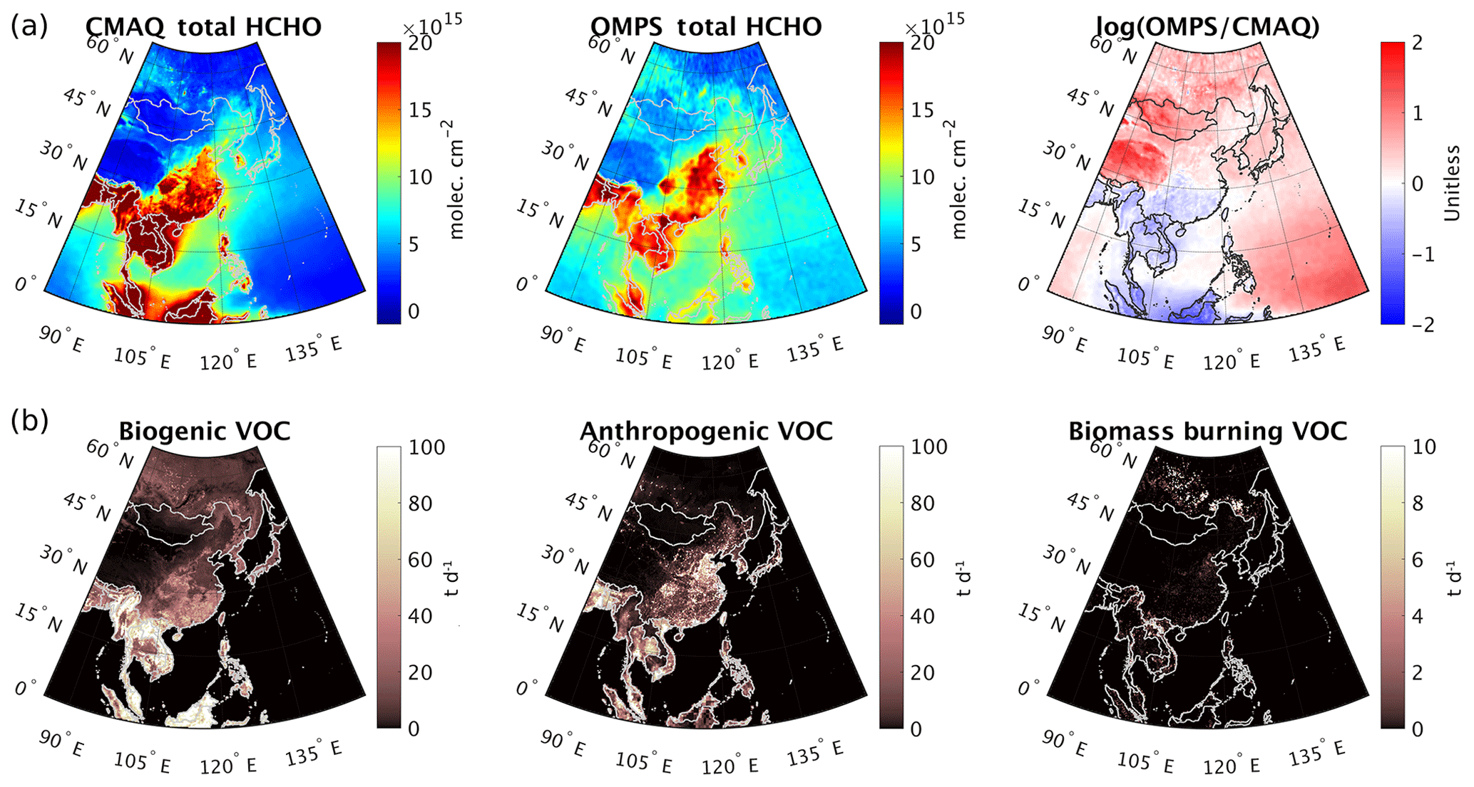
Figure 5 (a) HCHO total columns from the WRF-CMAQ model, OMPS (using adjusted AMFs based on the shape factors derived from the model and bias-corrected following the method proposed in Zhu et al., 2020), and the natural logarithmic ratio of OMPS ∕ CMAQ during May–June 2016 at ∼13:30 LST. (b) The major sources of VOC emissions in the area including biogenic emissions simulated by MEGAN, anthropogenic emissions estimated by MIX-Asia (2010), and biomass burning emissions made by FINN. The emissions are the daily mean values based on the emissions in May–June. The VOC emissions only add up those compounds that are included in the CB05 mechanism.

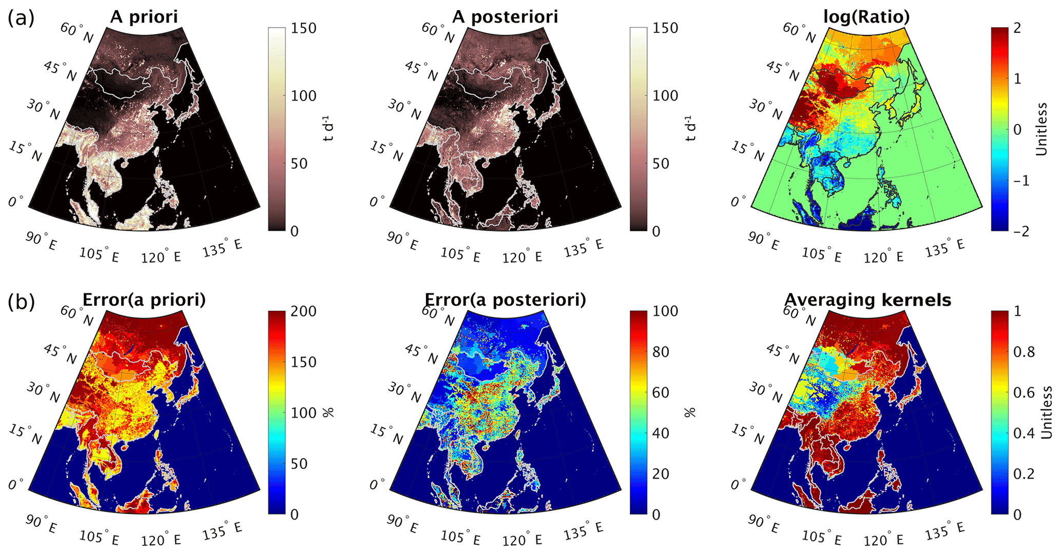
Figure 6 (a) Total VOC emissions (i.e., the a priori) constrained by the satellite observations (i.e., the a posteriori) in May–June 2016 and the natural logarithmic ratio of the a posteriori to the a priori. (b) The errors in the a priori based on Table 3, the errors in the top-down estimation, and the averaging kernels (AKs) obtained from the estimation.

Figure 6 illustrates the total VOC emissions before and after the inversion along with their errors. Immediately apparent is the large reduction of VOC emissions in the tropics and subtropics due to the overestimation of isoprene from MEGAN v2.1. In contrast, enhancements of the emissions are evident at higher latitudes. We observe that the dominantly anthropogenic VOC emissions over NCP increase (∼25 %) after the adjustment. Despite the presence of vegetation over Japan and South Korea, we do not see that the emissions are severely overestimated. Hence, the overestimation of isoprene emissions is more pronounced in the tropics, possibly because of an overestimation in the emission factors used for specific plants. Nevertheless, a nontrivial oversight in models could be an insufficient representation of both HO_x chemistry and dry deposition in forest canopies (Millet et al., 2008); as a result, the net amount of HCHO in the atmosphere over forest areas is higher than it should be if removal through either a chemical loss or faster dry deposition was considered.

Owing to the fact that we assume anthropogenic VOC emissions to be less uncertain relative to other sectors, the errors in the a priori are smaller in populated areas. We observe that OMPS HCHO columns are able to significantly reduce the uncertainty associated with the total VOC emissions over areas showing a strong HCHO signal (> 10¹⁶ molec. cm⁻²). Over clean areas, it is the other way around; we see less confidence in our top-down estimate (AK < 0.4) in areas such as Tibet and Mongolia.

We then compare the simulated HCHO column using two different emission inventories with those of OMPS in Fig. 7. We observe a substantial improvement in both the spatial structure and the magnitude of simulated HCHO columns using the a posteriori with respect to OMPS. The two-dimensional Pearson correlation increases from 0.78 to 0.91 after applying the adjustments to the emissions. In response to the increases in the total VOC emissions over the NCP, we observe ∼11 % enhancements in the simulated HCHO total columns. The updated emissions lead to a reduction in HCHO total columns as large as 70 % in the tropics.

Figure 7 (a–c) HCHO total columns from OMPS, the WRF-CMAQ simulated with the prior emissions, and the same model but with the top-down emissions constrained by the satellites in May–June 2016.

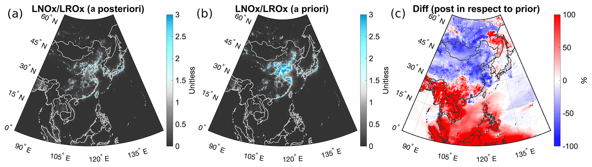
Figure 8 (a–c) Ratio of LNO_x∕LRO_x simulated by the posterior emissions, the prior, and their relative differences at 12:00–18:00 CST, averaged over May–June 2016 over the surface.

Validation of the model in terms of VOCs is not a straightforward task because the chemical mechanism used for our model has lumped several VOC species such as terminal or internal olefin or paraffin, only a handful of which were measured during the campaign. Also, the MIX-Asia inventory estimates the anthropogenic emissions for a selected number of VOCs in the CB05 mechanism. Here, we focus only on six compounds including isoprene, HCHO, ethene, ethane, acetaldehyde, and methanol, whose emissions are adjusted (with the same factor) based on satellite measurements. The comparison of the simulated values with the DC-8 measurements showed a noticeable mitigation in the discrepancy between two datasets at lower boundaries (< 900 hPa) in terms of isoprene (Fig. S5), ethane (Fig. S6), ethene (Fig. S7), and acetaldehyde (Fig. S8). Surprisingly, we observe a large underestimation of methanol over the Korean Peninsula by a factor of 10 (Fig. S9). The same tendency was observed in other regions in Wells et al. (2014) (see Fig. 8 in the paper). Our inversion obviously fails at mitigating the bias as there is not much direct constraint from the satellite observations on this compound. Wells et al. (2014) and Hu et al. (2011) demonstrated that methanol can be a secondary source of HCHO up to 10 %–20 % in midlatitudes in warm seasons. We tend to underestimate HCHO concentrations (by 15 %) in the lower atmosphere (< 900 hPa) after using the a posteriori over the Korean Peninsula (Fig. S10).

5 Implications for surface ozone

The results we have generated can be further exploited to elucidate changes in the ozone production rates, P(O₃), due to having the constrained NO_x and VOC emissions. We calculate P(O₃) by subtracting the ozone loss driven by HO_x (HO+HO₂), reaction with several VOCs (i.e., alkenes and isoprene), the formation of HNO₃, and O₃ photolysis followed by the reaction of O(¹D) with water vapor from the ozone formation via the removal of NO through HO₂ or RO₂:

$$\begin{array}{}\text{(8)}& \begin{array}{rl}& \mathrm{P}\left({\mathrm{O}}_{\mathrm{3}}\right)=k_{{\mathrm{HO}}_{\mathrm{2}}+\mathrm{NO}}\left[{\mathrm{HO}}_{\mathrm{2}}\right]\left[\mathrm{NO}\right]+\sum k_{{\mathrm{RO}}_{\mathrm{2},i}+\mathrm{NO}}\left[{\mathrm{RO}}_{\mathrm{2},i}\right]\\ & \left[\mathrm{NO}\right]-k_{\mathrm{OH}+{\mathrm{NO}}_{\mathrm{2}}+\mathrm{M}}\left[\mathrm{OH}\right]\left[{\mathrm{NO}}_{\mathrm{2}}\right]\left[\mathrm{M}\right]-k_{{\mathrm{HO}}_{\mathrm{2}}+{\mathrm{O}}_{\mathrm{3}}}\left[{\mathrm{HO}}_{\mathrm{2}}\right]\\ & \left[{\mathrm{O}}_{\mathrm{3}}\right]-k_{\mathrm{OH}+{\mathrm{O}}_{\mathrm{3}}}\left[\mathrm{OH}\right]\left[{\mathrm{O}}_{\mathrm{3}}\right]-k_{\mathrm{O}\left({}^{\mathrm{1}}\mathrm{D}\right)+{\mathrm{H}}_{\mathrm{2}}\mathrm{O}}\left[\mathrm{O}\left({}^{\mathrm{1}}\mathrm{D}\right)\right]\\ & \left[{\mathrm{H}}_{\mathrm{2}}\mathrm{O}\right]-\mathrm{loss}\left({\mathrm{O}}_{\mathrm{3}}+\mathrm{VOCs}\right).\end{array}\end{array}$$

Since P(O₃) is a nonlinear function of NO_x and VOC emissions, it is advantageous to look at the ratio of the chemical loss of NO_x to that of RO_x (RO₂+HO₂), a robust indicator pinpointing underlying drivers for the RO_x cycle. LRO_x is defined through the sum of primarily radical–radical reactions:

$$\begin{array}{}\text{(9)}& \begin{array}{rl}{\mathrm{LRO}}_x& =k_{{\mathrm{HO}}_{\mathrm{2}}+{\mathrm{HO}}_{\mathrm{2}}}{\left[{\mathrm{HO}}_{\mathrm{2}}\right]}^{\mathrm{2}}+\sum k_{{\mathrm{RO}}_{\mathrm{2},i}+{\mathrm{HO}}_{\mathrm{2}}}\left[{\mathrm{RO}}_{\mathrm{2},i}\right]\\ & \left[{\mathrm{HO}}_{\mathrm{2}}\right]+\sum k_{{\mathrm{RO}}_{\mathrm{2},\mathrm{i}}+{\mathrm{RO}}_{\mathrm{2},\mathrm{i}}}{\left[{\mathrm{RO}}_{\mathrm{2},i}\right]}^{\mathrm{2}}.\end{array}\end{array}$$

LNO_x mainly occurs via the NO₂+OH reaction:

$$\begin{array}{}\text{(10)}& {\mathrm{LNO}}_x=k_{\mathrm{OH}+{\mathrm{NO}}_{\mathrm{2}}+\mathrm{M}}\left[\mathrm{OH}\right]\left[{\mathrm{NO}}_{\mathrm{2}}\right]\left[\mathrm{M}\right].\end{array}$$

Typically, a value of LNO_x∕LRO_x ∼2.7 defines the transition line between VOC-sensitive and NO_x-sensitive regimes (Schroeder et al., 2017; Souri et al., 2020a).

Figure 8 depicts a contour map of LNO_x∕RO_x ratios over the surface before and after the inversion. As expected, the larger ratios are confined within major cities or industrial areas due to abundant NO_x emissions. The hotspot of VOC-sensitive regimes is located in NCP and YRD. Also of interest in Fig. 8 is that advection renders a major fraction of the Yellow Sea (the sea connecting China to Korea) VOC-sensitive. Using the a posteriori leads to precipitous changes in the chemical regimes. As a result of a large reduction in the isoprene emissions in both the tropics and subtropics, we observe a shift toward VOC-limited, though the values of LNO_x∕RO_x are still too far from the transition line (i.e., ≪2.7). The substantial reduction in NO_x emissions and an increase in VOC emissions over NCP and YRD go hand in hand for transitioning towards an NO_x-sensitive regime. The ratios over South Korea and Japan are found to be variable and somehow in sync with the changes in NO_x emissions.

The resultant changes in the LNO_x∕LRO_x ratios shed some light on ozone sensitivity with respect to its major precursors, but P(O₃) is also dependent on the absolute values of emissions, the degree of reactivity of VOCs, and the abundance of radicals. Here we use the integrated reaction rates (IRRs) to determine the most influential reactions pertaining to ozone loss and production at the surface. We focus on 12:00 to 18:00 China standard time (CST). Figure 9 shows the differences in the major pathways for the loss and formation of ozone at the surface within the time window. The differences are computed based on the subtraction of the simulation with the a posteriori from that with the a priori. In Fig. 9 we see a strong degree of correlation between changes in the magnitude of P(O₃) through the HO₂+NO reaction with those of NO_x emissions (Fig. 3), whereas changes in the magnitude of P(O₃) via the RO₂+NO reaction are primarily on par with those of VOC emissions (Fig. 6). We observe P(O₃) increases through HO₂+NO and RO₂+NO reactions in Japan, South Korea, Myanmar, and the Philippines because of increases in NO_x emissions in NO_x-sensitive regions. The simultaneous decrease in NO_x and VOC in PRD and Taiwan causes the production of ozone via the same pathways to reduce it.

Figure 9 Differences between the simulations with the updated emissions and the default ones of six major pathways of ozone production and loss over the surface. The time period is May–June 2016, 12:00–18:00 CST.

Normally, in VOC-rich environments, a reduction in VOC emissions boosts OH concentrations (Fig. S11). Consequently, we observe an enhancement of NO₂+OH reaction in the tropics and subtopics. A substantial reduction in the chemical loss of ozone through NO₂+OH over NCP and YRD arises from a considerable decrease in NO_x emissions and an increase in OH (due to chemical feedback of NO_x). In response to an increase in HO_x concentrations over NCP (Figs. S11–S12), we observe an enhancement of ozone loss through O₃+HO_x. The ozone photolysis (O¹D+H₂O) is majorly driven by photolysis and water vapor mixing ratios, both of which are roughly constant in both simulations; accordingly, the difference map of O¹D+H₂O is mainly reflecting changes in ozone concentrations (shown later). Interestingly, we observe a large reduction in the loss of ozone through reaction with VOCs at lower latitudes. This is essentially because of the reduction in ISOP+O₃, a VOC that prevails in those latitudes. Despite a much slower reaction rate for ISOP+O₃ compared to ISOP+OH and ISOP + hv (Karl et al. 2004), this specific chemical pathway can be important as a way to oxidize isoprene and form HO_x in forests (Paulson and Orlando, 1996).

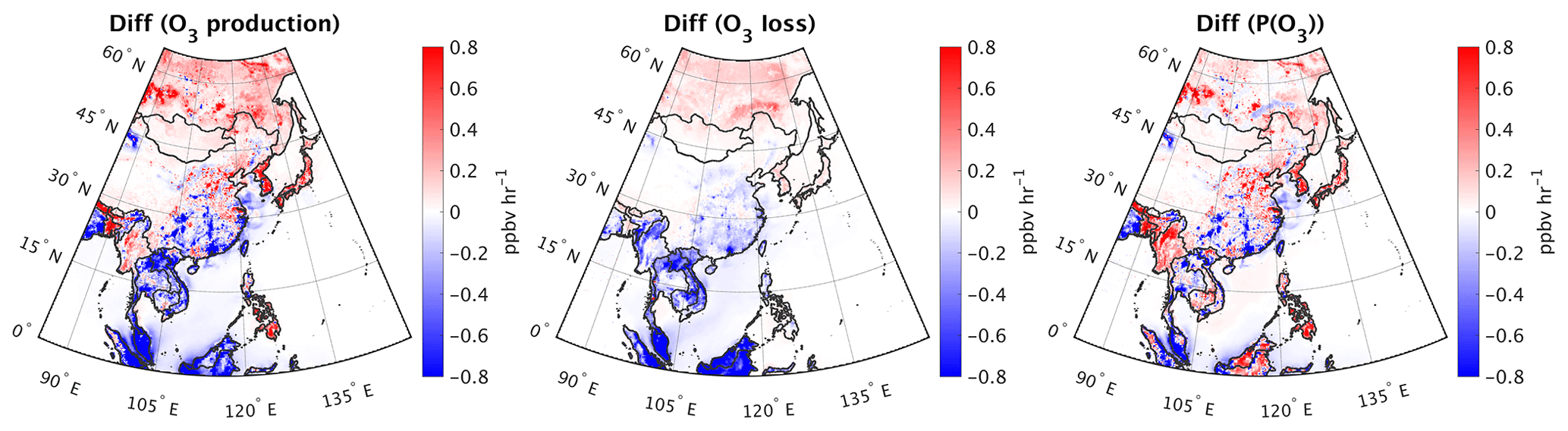
Figure 10 Changes in the major chemical pathways of ozone production and loss over the surface, as well as the net ozone production P(O₃) after updating the emissions. The time period is May–June 2016, 12:00-18:00 CST.

Figure 10 sums the differences of all mentioned chemical pathways involved in the formation and loss of surface ozone at 12:00–16:00 CST. Because of a complex nonlinear relationship between P(O₃) and its precursors, we observe large variability in both the sign and the amplitude of P(O₃). On average, changes in O₃ production dominate over changes in O₃ sinks except in Malaysia, which underwent a significant reduction in isoprene emissions, thus slowing down the ISOP + O₃ reaction. In general, the differences in P(O₃) follow the changes in the NO_x emissions depending on which chemical regimes prevail.

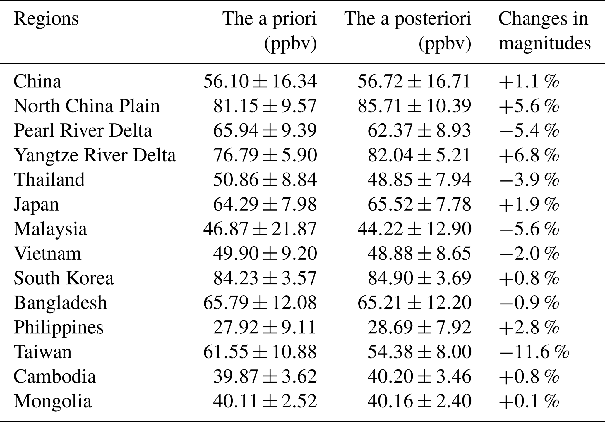
Much of the above analysis is based on ozone production rates; however, various parameters encompassing dry deposition, vertical diffusion, and advection can also affect ozone concentrations. Therefore, we further compute the difference between the simulated maximum daily 8 h average (MDA8) surface ozone levels before and after the inversion depicted in Fig. 11. For comparison, we also over-plot the Chinese air quality monitoring network observations (https://quotsoft.net/air/, last access: 2 June 2020) to have a general grasp of the performance of the model before and after adjusting the emissions. We see a striking correlation between P(O₃) (right panel in Fig. 10) and MDA8 surface ozone, indicating that the selected chemical pathways in this study can explain ozone changes. Nonetheless, the transport obviously plays a vital role in the spatial variability associated with the differences of surface ozone (e.g., Souri et al., 2016b). Figure 11 suggests a significant enhancement of ozone over NCP (∼4.56 ppbv, +5.6 %) and YRD (5.2 ppbv, +6.8 %) due to simultaneous decreases and increases in NO_x∕VOCs, which is in agreement with K. Li et al. (2019). On the other hand, reductions in NO_x mitigate ozone pollution in PRD (−5.4 %), Malaysia (−5.6 %), and Taiwan (−11.6 %). Table 6 lists the simulated MDA8 surface ozone levels for several regions before and after updating the emissions. Increases in MDA8 ozone over NCP and YRD overshadow decreases in southern China, resulting in a 1.1 % enhancement of ozone over China. This provides strong evidence that regulations on cutting VOC emissions should not be ignored. The largest reduction and increase in MDA8 ozone are found over Taiwan and YRD, respectively. Comparisons with surface observations show that the model generally captured the ozone spatial distributions; however, it tends to largely overpredict MDA8 surface ozone (∼7 ppbv). This tendency has been well-documented in other studies (e.g., Travis et al., 2016; Souri et al., 2017b; Lu et al., 2019). The updated simulation with the top-down emission partly reduces this overestimation in southern regions of China, while it further exacerbates the overestimation in the northern parts. No doubt much of this stems from the fact that the preexisting biases associated with the model (beyond emissions such as vertical mixing and cloud optical thickness) mask any potential improvement expected from the constrained emissions. Because of this, in addition to adjusting relevant emissions, a direct assimilation of ozone concentrations should complementarily be exploited (e.g., Miyazaki et al., 2019) to bolster the capability of the model to simulate ozone.

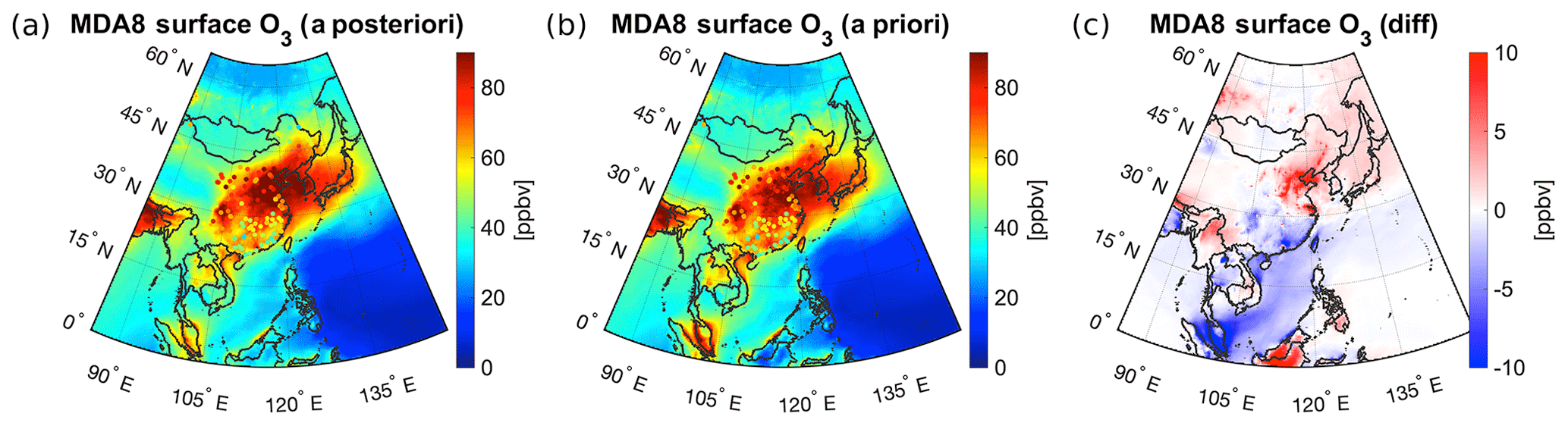
Figure 11 Simulated MDA8 surface ozone using the updated emissions constrained by OMI and OMPS observations (a), the default ones (b), and their difference (c) in May–June 2016. We over-plot surface MDA8 ozone values (circles) from the Chinese air quality monitoring network (https://quotsoft.net/air/, last access: 2 June 2020).

Table 6 MDA8 surface ozone levels before and after carrying out the inversion for different regions in May–June 2016.

6 Summary

In this paper we have focused on providing a top-down constraint on both volatile organic compound (VOC) and nitrogen oxide (NO_x) emissions using a combination of the error-characterized Smithsonian Astrophysical Observatory (SAO) Ozone Mapping and Profile Suite Nadir Mapper (OMPS-NM) formaldehyde (HCHO) and National Aeronautics and Space Administration (NASA) Ozone Monitoring Instrument (OMI) nitrogen dioxide (NO₂) retrievals during the Korean and United States (KORUS) campaign over East Asia in May–June 2016. Here, we include biogenic, biomass burning, and anthropogenic emissions from MEGAN, FINN, and the MIX-Asia 2010 inventory, respectively. A key point is that by considering the satellite observations together, we not only implicitly take the chemical feedback between HCHO–NO_x and NO₂–VOC into account by iteratively optimizing analytical nonlinear inversion, but we also quantify the impact of recent changes in emissions (since 2010) on surface ozone pollution.

Concerning total NO_x emissions, the inversion estimate suggests a substantial reduction over China (−23 %), North China Plain (NCP) (−32 %), Pearl River Delta (PRD) (−36 %), Yangtze River Delta (YRD) (−41 %), Taiwan (−23 %), and Malaysia (−22 %) with respect to the values reported in the prior emissions mostly dictated by the MIX-Asia 2010 inventory. In essence these values reflect recent actions to lower emissions in those countries (Zhang et al., 2012; Trappey el al., 2012; Chua and Oh, 2011). The analytical inversion also paves the way for estimating the averaging kernels (AKs), thereby indicating the amount of information acquired from satellites for the top-down estimation. We observe AKs > 0.8 over major polluted areas, indicating that OMI is able to improve the emission estimates over medium- to high-emitting regions. Conversely, AKs are found to be small over pristine areas, suggesting that little information can be gained from the satellite over rural areas given retrieval errors. In line with the studies of Irie et al. (2016) and Souri et al. (2017a), we observe a growth in the total NO_x emissions in Japan (+12 %) and South Korea (+9 %), which are partially explained by the new construction of thermal power plants in Japan and an upward trend in the number of diesel vehicles in South Korea.

MEGAN v2.1 estimates too much isoprene emission in the tropics and subtropics, a picture that emerges from the latitudinal dependence of the posterior VOC emissions on the prior ones. It is readily apparent from the top-down constrained VOC emissions that the prevailing anthropogenic VOC emissions in NCP are underestimated by 25 %, a direction that is in agreement with studies by Souri et al. (2017a) and Shen et al. (2019). We find that OMPS HCHO columns can greatly reduce the uncertainty associated with the total VOC emissions (AKs > 0.8) over regions having a moderate to strong signal (> 10¹⁶ molec. cm⁻²).

Large spatial variability associated with both NO_x and VOC results in great oscillation in chemical condition regimes (i.e., NO_x-sensitive or VOC-sensitive). Due to a considerable reduction and increase in NO_x∕VOC emissions in NCP and YRD, respectively, we observe a large increase (53 %) in the ratio of the chemical loss of NO_x (LNO_x) to the chemical loss of RO_x (RO₂+HO₂), shifting the regions towards NO_x-sensitive. As a result, a substantial reduction in the afternoon NO₂+OH reaction rate (a major loss of O₃) and an increase in afternoon NO+HO₂ and RO₂+NO (a major production pathway for O₃) are observed, leading to enhancements of the simulated maximum daily 8 h average (MDA8) surface ozone concentrations by ∼5 ppbv. Therefore, additional regulations on VOC emissions should be implemented to battle ozone pollution in those areas. On the other hand, being predominantly in NO_x-sensitive regimes favors regions including Taiwan, Malaysia, and PRD to benefit from reductions in NO_x, resulting in noticeable decreases in simulated MDA8 surface ozone levels. The comparison of simulated ozone before and after adjusting emissions and Chinese surface air quality observations reveals a large systematic positive bias (∼7 ppbv), which hinders attaining benefits from a more accurate ozone production rate due to the observationally constrained NO_x∕VOC ratios. This highlights the need to explicitly deal with other underlying issues in the model (e.g., Travis et al., 2016) to be able to properly simulate surface ozone.

It has taken many years to develop satellite-based gas retrievals and weather and chemical transport models accurate enough to enable observationally based estimates of emissions with reasonable confidence and quantified uncertainty, as well as to produce credible top-down emission inventories over certain areas. However, it is essential to improve certain aspects to be able to narrow the range of uncertainty associated with the estimation, such as the following: (i) parameterizing the spatiotemporally varying bias of satellite gas retrievals; (ii) improving the knowledge of prior errors in bottom-up emissions; (iii) propagating model parameter errors such as PBL, radiation, and winds to the final output (e.g., Rodgers, 2000); and (iv) due to intertwined chemical feedback between various chemical compounds, inverse modeling needs to properly incorporate all available information (beyond HCHO and NO₂) considering the cross-relationship either explicitly or implicitly. Despite these limitations, this research demonstrated that a joint inversion of NO_x and VOC emissions using well-characterized observations significantly improved the simulation of HCHO and NO₂ columns, permitting an observationally constrained quantification of the response of ozone production rates to emission changes.