the Creative Commons Attribution 4.0 License.
the Creative Commons Attribution 4.0 License.
 | 13 Aug 2020
Reformulating the bromine alpha factor and equivalent effective stratospheric chlorine (EESC): evolution of ozone destruction rates of bromine and chlorine in future climate scenarios
Debra K. Weisenstein
Ross J. Salawitch
David M. Wilmouth
Future trajectories of the stratospheric trace gas background will alter the rates of bromine- and chlorine-mediated catalytic ozone destruction via changes in the partitioning of inorganic halogen reservoirs and the underlying temperature structure of the stratosphere. The current formulation of the bromine alpha factor, the ozone-destroying power of stratospheric bromine atoms relative to stratospheric chlorine atoms, is invariant with the climate state. Here, we refactor the bromine alpha factor, introducing normalization to a benchmark chemistry–climate state, and formulate Equivalent Effective Stratospheric Benchmark-normalized Chlorine (EESBnC) to reflect changes in the rates of both bromine- and chlorine-mediated ozone loss catalysis with time. We show that the ozone-processing power of the extrapolar stratosphere is significantly perturbed by future climate assumptions. Furthermore, we show that our EESBnC-based estimate of the extrapolar ozone recovery date is in closer agreement with extrapolar ozone recovery dates predicted using more sophisticated 3-D chemistry–climate models than predictions made using equivalent effective stratospheric chlorine (EESC).
- Article
(1450 KB) - Full-text XML
- BibTeX
- EndNote


Anthropogenic emissions of ozone-destroying halocarbons have declined significantly since the implementation of the Montreal Protocol on Substances that Deplete the Ozone Layer (and its subsequent amendments); however, stratospheric inorganic halogen inventories still remain elevated relative to levels prior to the first observations of the seasonal Antarctic ozone hole due to the exceptionally long lifetimes of the precursor compounds for inorganic halogen. Recovery of the halogen content of the stratosphere to the levels representative of the benchmark year 1980 is estimated to occur some time around the year 2060 in the extrapolar regions (Newman et al., 2006; Engel et al., 2018a, b); however, 3-D chemistry–climate model (CCM) simulations predict ozone recovery dates up to 2 decades sooner (Dhomse et al., 2018; Braesicke et al., 2018) as halogen inventory recovery is an imperfect proxy for ozone recovery.
The vast majority of inorganic chlorine in the lower stratosphere is present in the reservoir forms HCl and ClONO2. The gas-phase reaction of these two reservoirs is too slow to be of atmospheric importance; however, heterogeneous reactions on the surfaces of stratospheric aerosols (Solomon et al., 1986; Brasseur et al., 1990) can be fast enough to enable chlorine activation and ClOx-mediated ozone depletion cycling. It is typical that only a few percent of inorganic chlorine is present in the active forms in the lower stratosphere because conversion of the Cl radical back to the inorganic reservoir can be quite fast, limiting the chain length (and it follows, the extent of ozone loss) of mechanisms involving chlorine alone in this region of the stratosphere.
Mechanisms of BrOx-mediated ozone depletion are much less sensitive to the surrounding environment than mechanisms mediated by ClOx. This is because inorganic reservoirs of bromine are significantly less stable, enhancing the quantity of reactive halogen available for ozone processing. Bromine is up to 2 orders of magnitude more likely to be found in its active form than chlorine, depending on the physicochemical environment (Wofsy et al., 1975; Salawitch et al., 2005). Additionally, unlike the catalytic cycles of chlorine, in which the extent of ozone loss following the addition of chlorine atoms is limited by the relatively short chain length of the catalytic center, catalytic processing of ozone facilitated by the addition of bromine is potentiated due to its greater (up to orders of magnitude in difference) chain effectiveness (Lary, 1997). The bromine interfamily ozone destruction cycles are responsible for a similarly sized fraction of global lower stratospheric ozone loss as the chlorine cycles (Salawitch et al., 2005; World Meteorological Organization, 2018; Koenig et al., 2020). This large fractional share of ozone destruction chemistry occurs despite the fact that bromine is approximately 2 orders of magnitude less abundant than chlorine as a consequence of (a) the larger fraction of reactive bromine available at a given mixing ratio and (b) the catalytic reaction channels made accessible by the weaker bromine–oxygen molecular bond (Yung et al., 1980; McElroy et al., 1986; Brune and Anderson, 1986).
The bromine alpha factor, αBr, is a metric that quantifies the ozone-depleting efficiency of a bromine atom relative to chlorine. This quantity is defined either as the ratio of ozone loss processing rates, as in Eq. (1), or as the ratio of the overall change in ozone abundance on a per-halogen-atom basis per Eq. (2). In both formulations, αBr is computed as a function of calendar date, t, and location in the atmosphere, ρ. Daniel et al. (1999) demonstrate that both equations provide identical results when changes in ozone are dominated by chemical rather than dynamical processes.
Values of αBr vary strongly as a function of pressure, latitude, and season. This variance is primarily a function of (a) chemical environment, (b) prevailing actinic flux, (c) aerosol surface area, and (d) temperature (Solomon et al., 1992; Danilin et al., 1996; Ko et al., 1998; Daniel et al., 1999). Frequently, αBr is reported as an effective value for the stratospheric column, computed in a similar manner as in Eqs. (1) or (2), the key difference being that ρ represents the position of the stratospheric column. Likewise, it is common to provide a regional annual average column αBr, which is computed as the average of column αBr values for all locations within a specified region across a calendar year. Global annual average column values for αBr are currently estimated between 60 and 65, depending on the model employed and the chemistry–climate boundary conditions (Engel et al., 2018b; Sinnhuber et al., 2009). Values of αBr tend toward a minimum at the Equator, maximizing in the boreal summer. Denitrification and heterogeneous activation produce a minimum in αBr during the austral springtime. In vertical profiles, αBr tends to maximize in the lower stratosphere where reactive chlorine is less prevalent than in the middle stratosphere.
The quantity αBr is especially useful for the determination of parameterized estimates of the budget of reactive inorganic halogens given a mixture of halogen-containing halocarbons of an arbitrary mean age, as in the metric of equivalent effective stratospheric chlorine (EESC). This quantity expresses the ozone-depleting power of a parcel of well-mixed stratospheric trace gases as a function of the mean stratospheric age of the parcel, Γ, and the trace gas background of the stratosphere at time t (Daniel et al., 1995; Newman et al., 2007). Equation (3) provides the most recently suggested formulation of EESC, in which is the trend-independent fractional release factor for species i for a parcel of air with mean age Γ, which contains ni, Cl chlorine atoms and ni, Br bromine atoms, scaled by αBr(t, Γ), where it is assumed that Γ can serve as a proxy for ρ (Ostermöller et al., 2017; Engel et al., 2018a). Inside the integral, the mixing ratio of species i is computed for each element comprising the age spectrum and normalized to the contribution of that element to the age spectrum. The tropospheric mixing ratio of species i, χ0, i is adjusted to account for transit time within the stratosphere, t′, and multiplied by the normalized release-weighted transit time distribution, , where is the mean age of halogen atom release.
EESC is frequently employed to constrain the date of stratospheric ozone recovery, often by using graph theory to determine when stratospheric chlorine levels will return to the levels observed in 1980 as a benchmark (Newman et al., 2006; Engel et al., 2018b). The technique is fast and simple: EESC is calculated as a function of location in the stratosphere (for which Γ is a proxy) and future date, following which a horizontal line is propagated in time at the value of EESC in 1980, and the intercept of the two traces is interpreted as the date of halogen recovery (and, it follows, an approximate date of ozone recovery). The extrapolation is built on the assumptions that, as the climate evolves, (1) the alpha factor remains constant and (2) the amount of ozone destroyed by chlorine, on a per-chlorine-atom basis, also remains constant. However, projections of the future physicochemical state of the stratosphere do not necessarily provide for these two assumptions to be true. Indeed, the envelope of future projections (e.g., Representative Concentration Pathway (RCP) and Shared Socioeconomic Pathway (SSP) scenarios) of emissions of CH4, N2O, and CO2, among other relevant species, indicates that it is nearly certain that these two assumptions will not be true, especially in the extrapolar stratosphere.
Significant variations between different climate models and possible states of the future atmosphere limit the skill level of model simulations in predicting ozone recovery dates (Charlton-Perez et al., 2010). These large uncertainties notwithstanding, it is understood that there may be a super-recovery of global stratospheric ozone in the future as EESC declines, the Brewer–Dobson circulation accelerates, and the stratosphere cools (Austin and Wilson, 2006; Li et al., 2009; Eyring et al., 2013; Banerjee et al., 2016; Chiodo et al., 2018). The extent of super-recovery can be attributed to both photochemical and dynamical factors. Future ozone abundance is expected to be controlled by photochemical factors in the middle to upper stratosphere. The degrees by which photochemical rates of bimolecular ozone loss processes are slowed and the rate at which the termolecular formation of ozone is increased are a result of (a) local radiative cooling due to the enhancement of the stratospheric burden of anthropogenic greenhouse gases and (b) chemical suppression of ozone loss cycling due to reactive anthropogenic greenhouse gas emission (Rosenfield et al., 2002; Waugh et al., 2009; Oman et al., 2010; Eyring et al., 2013). In the lower stratosphere, where the photochemical lifetime of ozone is large, the expected super-recovery is dominated by dynamical factors, such as the model response of the Brewer–Dobson circulation to greenhouse gas perturbation, which alters both the stratospheric lifetime of long-lived inorganic halogen precursors and the transport of ozone from the tropics where it is produced (Butchart et al., 2006; Plummer et al., 2010; Zubov et al., 2013).
Dhomse et al. (2018) provide constraints on the dates stratospheric ozone might recover to year 1980 benchmark thickness using a comprehensive multi-model framework (20 models, 155 simulations) spanning multiple greenhouse gas emissions scenarios, finding that while the date of Antarctic springtime recovery is most sensitive to Cly inventories, extrapolar column recovery dates (and to a lesser extent, the Arctic springtime recovery date) are highly sensitive to the greenhouse gas forcing applied. In their analysis, Dhomse et al. (2018) indicate that midlatitude ozone recovery will occur sooner in both hemispheres for scenarios with greater radiative forcing. When greenhouse gases are fixed, the dates projected for midlatitude recovery (∼2060) are in close agreement with the EESC-based estimates provided in Engel et al. (2018a) of 2059; however, greenhouse gas perturbations hasten projected midlatitude recovery dates in 3-D models by ∼10 years in the Northern Hemisphere and ∼20 years in the Southern Hemisphere (Eyring et al., 2010, 2013; Dhomse et al., 2018).
In this work, we present the first assessment of column αBr in future climate change scenarios. Additionally, we evaluate the sensitivity of column αBr to prescribed perturbations of reactive greenhouse gases while anthropogenic halocarbons slowly decay as the century progresses. We then refactor αBr such that parameterized estimates of ozone recovery can more accurately be related to the ozone-destroying power of the inorganic halogen content of the stratosphere given a particular benchmark date. Finally, we show that this method provides much better agreement with 3-D CCM estimates of ozone recovery to the 1980 benchmark date than EESC-based estimates.
Table 1Experiment schedulea.
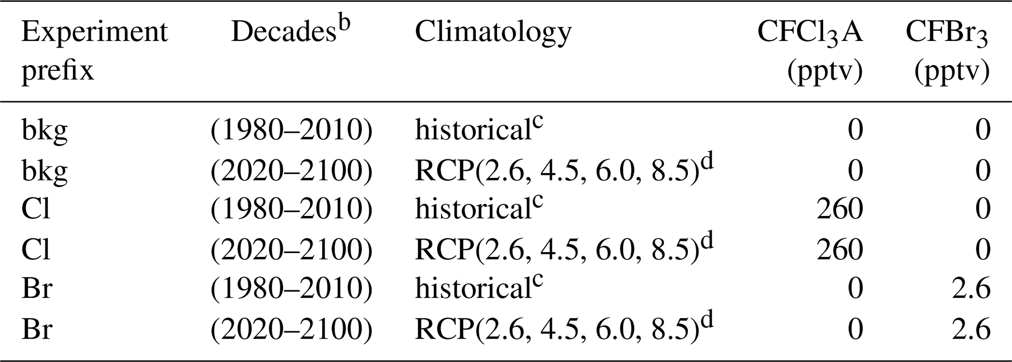
a All permutations of parenthetical parameters were evaluated. b Constant year for each decade (e.g., 1980, 1990, 2000). c Informed by Fleming et al. (1999). d Informed by Meinshausen et al. (2011) and Watanabe et al. (2011).
The AER-2D chemical transport model was employed with 19 latitudes (90∘ S–90∘ N) and 51 levels (1000–0.2 hPa) for this work (Weisenstein et al., 1997, 2007). The model includes 104 chemical species, accounting for Fy, Cly, Bry, Iy, NOy, HOx, Ox, SOx, and CHOx chemistry. Chemical reactions (314 kinetic reactions and 108 photochemical reactions) were computed using rate constants and cross sections as recommended in the most recent (2015) JPL data evaluation (Burkholder et al., 2015). Additionally, the model features fully prognostic aerosol microphysics and chemistry (e.g., nucleation, coagulation, condensation, evaporation, sedimentation, and heterogeneous chemical interactions in 40 sectional size bins). Future emissions of greenhouse gases were informed by the Representative Concentration Pathway framework (Van Vuuren et al., 2011; Meinshausen et al., 2011). Future climatological boundary conditions were obtained from the corresponding RCP experiments of MIROC-CHEM-ESM, an Earth system model with stratospheric chemistry. Future halocarbon inventories were informed by Table 6-4 of the 2018 WMO Scientific Assessment of Ozone Depletion (World Meteorological Organization, 2018) with an additional 5 pptv stratospheric bromine from very short-lived bromocarbons (Wales et al., 2018). Experiments performed in the historical past were informed by historical climatologies obtained from Fleming et al. (1999). Specified dynamics corresponding to the 1978–2004 climatological average were employed for all historical and future experiments and were prepared using data obtained from Fleming et al. (1999).
Halogen perturbation scenarios were prepared in the manner of Daniel et al. (1999). Specifically, bromine alpha factors were determined per Eq. (2), in which ozone deficits were computed by the column difference between control and halogen gas perturbation scenarios. CFC-11 proxy molecules (CFCl3A and CFBr3) were constructed to provide identical transport and release of a known quantity of halogen atoms (Br or Cl, depending on the prescribed perturbation) between runs. For bookkeeping purposes, this was done for both chlorine and bromine delivery (e.g., the molecule labeled CFCl3A has the same chemical kinetics and photolysis rates as CFC-11, providing three chlorine atoms upon decomposition, but can be perturbed in the model separately from CFC-11). Experiments were performed as outlined in Table 1, in which each permutation of the parenthetical parameters was evaluated, resulting in a total of 108 model realizations (2160 model years). Experiments of a certain scenario (e.g., for the year 2100 RCP8.5 experiment: bkg2100RCP8.5, Cl2100RCP8.5, Br2100RCP8.5) were initialized from identical 20-year chemical–climatological spun-up boundary conditions. Evaluations were conducted at constant chemical and climatological conditions (i.e., time-slice boundary conditions) corresponding to the last year of each decade (e.g., 1980, 1990, … , 2100). Perturbation and control experiments were evaluated over the course of 20 model years, a duration determined to be an appropriate period for the perturbation gas to reach chemical–dynamical steady state. Data analysis was conducted on the final 12 months of each experiment and control run. Perturbation gas surface mixing ratios were selected to produce global and local ozone depletion of less than 1 % in each climate state relative to the unperturbed condition to prevent instability in the chemical Jacobian.
The model performance and experiment design were validated using calculations of αBr in a chemistry–climate state representative of the year 2006. This climate condition has previously been evaluated for αBr (Sinnhuber et al., 2009) using the JPL-2006 photochemical–kinetics recommendations (Sander et al., 2006). Validation runs for this work were informed by either JPL-2006 or JPL-2015 photochemical–kinetics packages. A comparison of the two model evaluations is presented in Fig. 1 in which there is little qualitative difference in the annual variation in αBr between the JPL-2006 and JPL-2015 photochemical–kinetics packages. Implementation of JPL-2015 chemistry results in a general increase in column αBr of ∼10 relative to JPL-2006 contours in both polar and extrapolar regions. Our annually and globally averaged αBr of 67 in the JPL-2006 instance compares favorably to the results of Sinnhuber et al. (2009), who report an annually and globally averaged αBr of 64 in their analysis of the same chemistry–climate state using the same photochemistry and kinetics package. For the JPL-2015 evaluation, the annually and globally averaged αBr is 74, which is larger than previously reported values. These differences are likely the result of a combination of changes in chemical rates between JPL-2006 and JPL-2015, such as (a) a 2 % increase in the rate of Cl+CH4 at 200 K, (b) an 8 % increase in the formation rate of NO by N2O+O(1D) at 200 K, (c) a 4 % increase in the rate of Br+O3 at 200 K, (d) a 121 % increase in the rate of CHBr3+OH at 200 K, and (e) a 5 % increase in the rate of Cl+ClOOCl at 200 K.
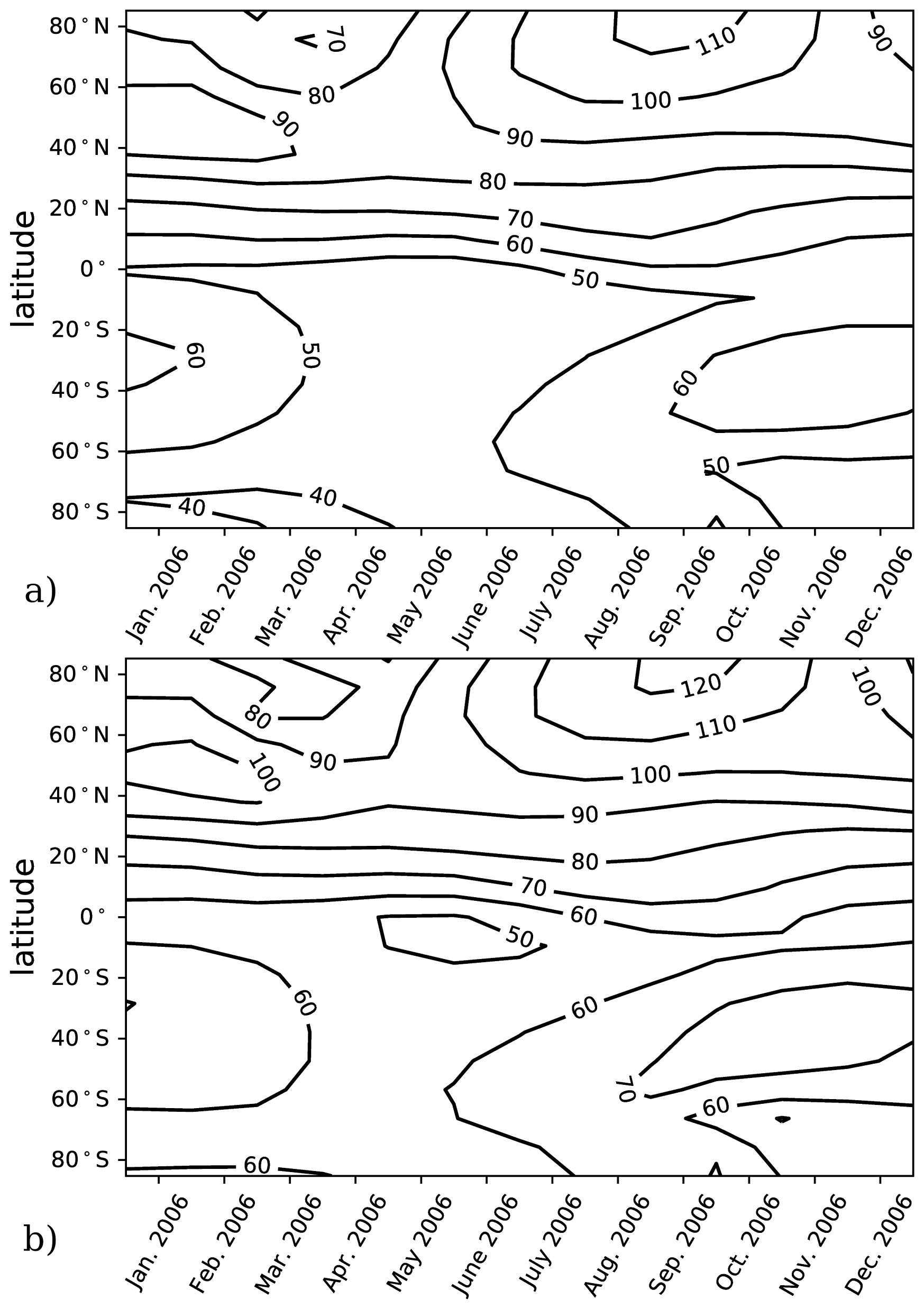
Figure 1Column αBr as a function of latitude and season for the year 2006. (a) Model results computed using JPL-2006 photochemistry and kinetics (Sander et al., 2006) for the year 2006. (b) Model results computed using JPL-2015 photochemistry and kinetics (Burkholder et al., 2015) for the year 2006.
3.1 Refactoring αBr: a new definition of EESC
Prior evaluations of αBr were computed with static chemistry–climate states. Because the relative ozone-processing rate of bromine to chlorine is likely to change with time, and also between chemistry–climate scenarios at the same point in time, we add a dependence on the chemistry–climate state, ξ, to the definition of αBr (Eq. 4).
We can then replace the climate-invariant αBr(t,Γ) in Eq. (3) with to produce a climate-sensitive EESC that accounts for changes in the relative ozone-destroying efficiency of bromine to chlorine (Eq. 5).
Furthermore, we recognize that the ozone-processing powers of chlorine and bromine are independently sensitive to changes in the physicochemical background of the stratosphere. The two variables must be separated in order to understand the evolution of the change in the processing power of chlorine and bromine as a function of the chemistry–climate state. To accomplish this, we define the eta factor, ηCl and ηBr, in Eqs. (6) and (7) as the ratio of the change in ozone following the addition of chlorine or bromine at time t, location ρ, and climate state ξ to the change in ozone following the same perturbation in a benchmark chemistry–climate state, Ξ. The eta factor thus expresses the ozone-depleting efficiency of a chlorine or bromine atom in an arbitrary chemistry–climate state relative to the ozone-depleting efficiency of a chlorine atom in the benchmark chemistry–climate state.
It is apparent that the definition of αBr given in Eq. (4) can be derived from ηBr and ηCl provided that the benchmark chemistry–climate state is identical between the two expressions (Eq. 8).
By substituting this refactored definition of αBr into Eq. (5) for the computation of EESC, we can now quantify the Equivalent Effective Stratospheric Benchmark-normalized Chlorine (EESBnC) (Eq. 9). The difference between EESC and EESBnC is significant; whereas EESC considers “the relative efficiency of chlorine and bromine for ozone depletion” (World Meteorological Organization, 2018), EESBnC accounts for the overall efficiency of chlorine and bromine relative to a benchmark chemistry–climate state. Thus, EESBnC provides the ozone-depleting power of an air parcel in the stratosphere propagated independently of changes in the rates of chlorine or bromine ozone loss catalysis.
3.2 Calculation of future RCP scenario α and η
Packaged within the definitions of α and η are both local (e.g., photochemical catalytic processing) and nonlocal influences on ozone abundance (e.g., dynamical effects, ozone layer self-healing effect, etc.), as illustrated in Eq. (10). These nonlocal factors do not cancel out in the evaluation of ηCl per Eq. (6) or ηBr per Eq. (7) as they do in the calculation of αBr per Eqs. (1) and (2) because the nonlocal factors at time t in some evolved climate state are not likely to be the same as they were during the benchmark time period.
To avoid this complication, we employ specified dynamics corresponding to the 1978–2004 climatological average in order to calculate only the photochemical component of the ozone tendency. These dynamics tend to produce less seasonal variation in αBr in the extrapolar Southern Hemisphere than in the extrapolar Northern Hemisphere, as depicted in Fig. 1. Because of the carefully controlled magnitude of the imposed ozone deficit (∼1 %), changes in ozone between experiment and control scenarios from all other effects can be assumed to be insignificant relative to the ozone changes produced by the chemical perturbation.
The temporal dependencies of the well-mixed greenhouse gases employed in the climatological perturbations are illustrated in Fig. 2, constructed from data provided by Meinshausen et al. (2011). Prescribed mixing ratios of CO2, which is chemically inert in this model and only perturbs ozone chemistry via thermal effects, are provided in panel (a). The trajectories of CH4 in panel (b) and N2O in panel (c) are particularly noteworthy because these species are closely coupled with the ozone steady state via changes in inorganic halogen reservoir inventories. In the instance of RCP8.5, CH4 increases nearly 2.5 times by the year 2100 from the 1980 mixing ratio, and N2O increases by a factor of 1.4 during the same time period. The reactive greenhouse gas situation in RCP2.6 is significantly different: CH4 mixing ratios decline by 19 % and N2O mixing ratios increase by 14 % during the period spanning the year 1980 and the year 2100. The intermediate scenarios, RCP4.5 and RCP6.0, both feature small end-of-century increases in CH4 mixing ratios of less than 10 % relative to the year 1980 value but with modest increases during the middle half of the 21st century. For RCP4.5 and RCP6.0, prescribed N2O emissions increase by 24 % and 35 %, respectively, over the same time interval.

Figure 2Surface mixing ratios of (a) CO2, (b) CH4, and (c) N2O as a function of time and RCP scenario. Data obtained from Meinshausen et al. (2011).
Table 2Values of extrapolar (60∘ S–60∘ N) , , and for historical and future scenarios.

a αBr calculated per Eq. (4). b ηCl calculated per Eq. (6) and ηBr calculated per Eq. (7), Ξ =1980. Historical temperature fields obtained from Fleming et al. (1999). Historical and future greenhouse gas emissions specified per Meinshausen et al. (2011). Future temperature fields derived from Watanabe et al. (2011).
Values of annually averaged extrapolar ηCl and ηBr (60∘ S–60∘ N) were computed on a decadal basis for every decade between 1990 and 2010 using historical data and for each decade between 2020 and 2100 for each RCP scenario. For all results reported in this work, the chemistry–climatology corresponding to the year 1980 was selected as the benchmark state (Ξ=1980). These values are presented, along with the corresponding alpha factors, in Table 2 for the historical period and for future scenarios. These results are also visualized in Fig. 3 for (a) extrapolar αBr, (b) extrapolar ηCl, and (c) extrapolar ηBr. It is immediately apparent that, while αBr deviates by less than 10 % from its 1980 value for all evaluated future atmospheres as presented in panel (d), the corresponding ηCl and ηBr values are generally observed to decline by a much more significant extent in panels (e) and (f), respectively.
We highlight the clear qualitative trends of decreasing ηCl and ηBr with climatological forcing scenario severity. Particular notice should be directed to results corresponding to RCP8.5, in which αBr does not demonstrate a significant coefficient of variation throughout the 21st century (CV(αBr) = 2.1 %), but η factors decline precipitously as the century progresses (CV(ηCl) = 14.3 % and CV(ηBr) = 14.5 %). This behavior follows the sensitivity expected when there is a large increase in N2O and CH4. A downward trend in αBr is observed as time propagates in RCP scenarios 2.6, 4.5, and 6.0. This effect is dominated by the declining availability of ClOx as a result of the slow decay of long-lived ozone-depleting substances. In the case of RCP2.6, a slight increase in ηCl occurs after the year 2040, driven by the continuous decline in the CH4 mixing ratio and the stabilization of the N2O mixing ratio in the scenario prescription.
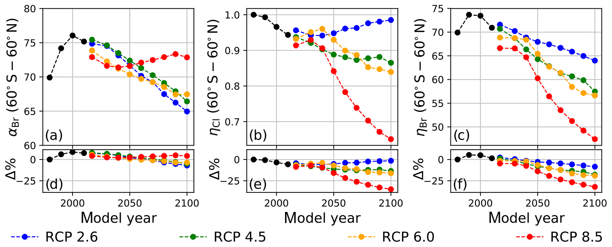
Figure 3Extrapolar α and η computed on a decadal basis as a function of RCP scenario. Black traces were calculated using historical boundary conditions. (a) αBr, (b) ηCl, and (c) ηBr. Percent differences of values in (a–c) relative to the year 1980 are presented in panels (d–f), respectively.
A sensitivity analysis was conducted on αBr, ηCl, and ηBr in order to clarify the differences presented in Fig. 3. In this analysis, αBr, ηCl, and ηBr were calculated in the manner previously described but with the chemistry–climate perturbation, ξ, identical to the chemistry–climate benchmark, Ξ, except for a single perturbed parameter. Four variables were perturbed separately: (a) N2O, (b) CH4, (c) the Bry∕Cly ratio, and (d) the temperature profile. For each perturbation experiment, all factors except for the perturbed factor were constrained to their year 1980 value(s). Perturbation values were intentionally selected to induce large variations in model response. For N2O and CH4, mixing ratios were scaled between preindustrial values and twice the RCP8.5 year 2100 value. Bry∕Cly ratios were selected to range between low values representative of the year 1990, moderate values representative of the year 2000, and high values representative of the year 2100 WMO Table 6-4 projections. Stratospheric temperature profile perturbations spanned a minimum as parameterized by the RCP8.5 year 2100 projection to a maximum value representative of the climatological average of the years 1978–2004.
Figure 4a demonstrates that αBr is only slightly sensitive to changes in the mixing ratio of N2O between preindustrial and 2× RCP8.5 year 2100 levels. Unlike αBr, both ηCl and ηBr, as shown in panels (e) and (i), decline monotonically and with nearly identical gradients, as both the bromine and chlorine cycles are suppressed through reactions with NOx. This suppression arises primarily via the direct formation of the halogen nitrate.
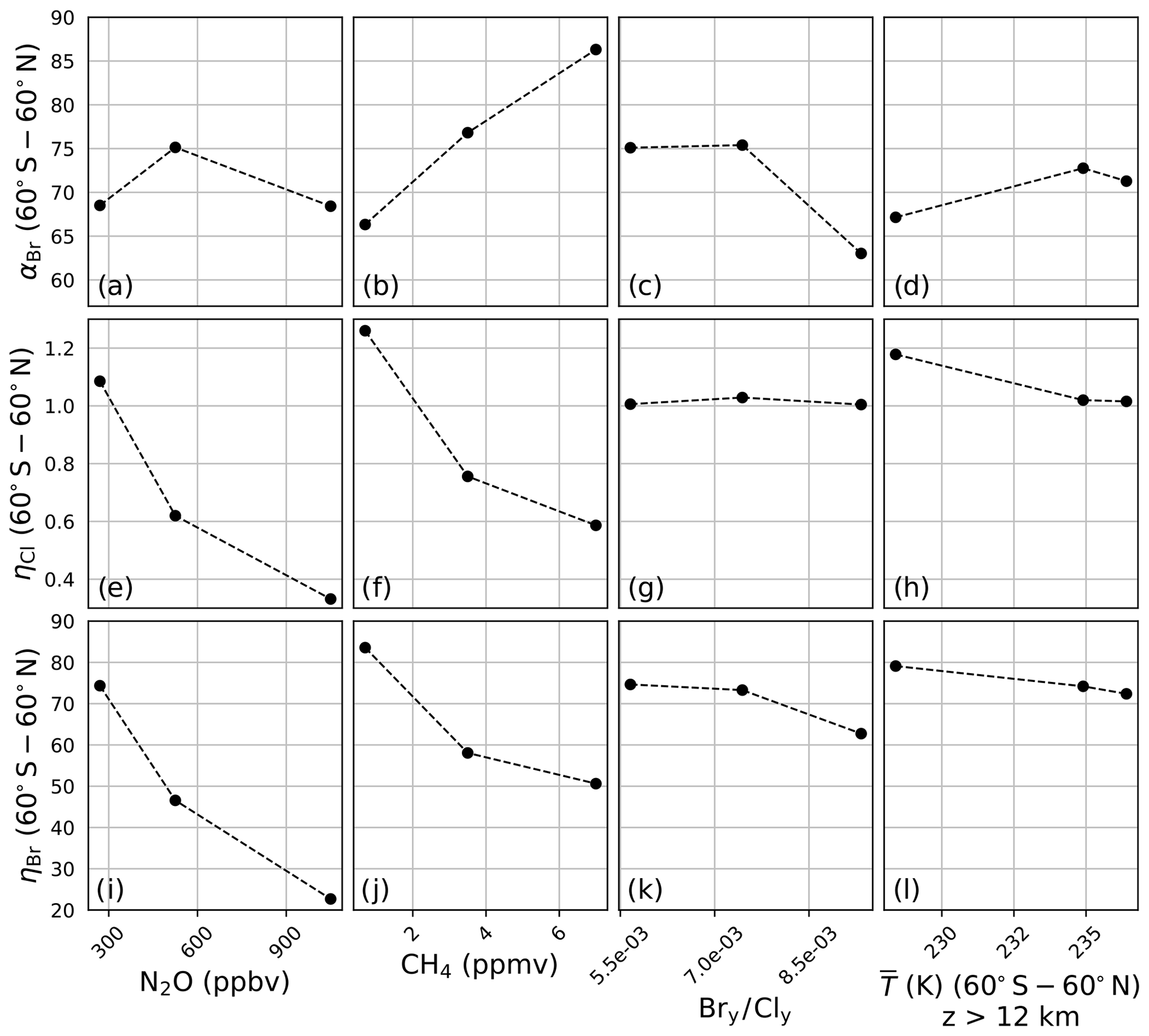
Figure 4Extrapolar α and η sensitivity to perturbation parameters. N2O: (a) αBr, (e) ηCl, (i) ηBr. CH4: (b) αBr, (f) ηCl, (j) ηBr. Bry∕Cly: (c) αBr, (g) ηCl, (k) ηBr. Temperature: (d) αBr, (h) ηCl, (l) ηBr.
Variation in the model output as a function of the mixing ratio of CH4 is presented in Fig. 4b, f, and j. Unlike the case of N2O, αBr (panel b) is a strong function of CH4, increasing as the mixing ratio is increased from the preindustrial value to 2× RCP8.5 year 2100 quantities. The reason for this behavior is made evident upon evaluation of ηCl and ηBr in panels (f) and (j). The reaction of Cl with CH4 is fast, forming the inorganic reservoir HCl, but the analogous reaction of Br with CH4 does not effectively occur. Despite these factors, some suppression of the bromine cycle does occur as a result of competition with enhanced HOx (from the oxidation of CH4) for a reduced quantity of ClOx reaction partners.
The effect of changing Bry∕Cly ratios was investigated over the range of 0.0057–0.0093. This range encapsulates the minimum and maximum ratios expected between the years 1980 and 2100 according to WMO 2018 Table 6-4. These values were computed according to Eq. (11) using the trend-independent fractional release factors of Engel et al. (2018a). The values of αBr, ηCl, and ηBr are presented in Fig. 4c, g, and k, respectively. Values of αBr are generally expected to decrease as the ratio of Bry∕Cly increases.
Both Chipperfield and Pyle (1998) and Danilin et al. (1996) demonstrated that αBr in the polar vortex is highly dependent on the relative mixing ratios of available bromine and chlorine, maximizing at low Bry∕Cly because of the enhanced abundance of ClO reaction partners for each BrO radical in those conditions. Within the polar vortex the fraction of ozone loss due to the chlorine peroxide cycle declines as Bry∕Cly increases; however, the extent of ozone depletion following the addition of bromine does not increase proportionately because the system is controlled by the chlorine abundance. While the same relationship between αBr and Bry∕Cly exists in the extrapolar stratosphere, the chemistry responsible for this effect is different. The higher temperatures of the extrapolar stratosphere render the chlorine peroxide cycle ineffective for the loss of ozone. We find that the extent of ozone loss following the addition of bromine increases significantly due to BrOx–ClOx and BrOx–HOx cycles, and we derive extrapolar αBr values as a function of Bry∕Cly, qualitatively consistent with the extrapolar results of Chipperfield and Pyle (1998).
Evaluations of the model in which stratospheric temperature profiles were varied between RCP8.5 year 2100 (low), RCP2.6 year 2030 (medium), and 1978–2004 climatological averages (high) demonstrate a dampened sensitivity of αBr, as presented in Fig. 4d, in which αBr increases by only 6 % from the coldest scenario to the warmest scenario. Heterogeneous activation of chlorine in the coldest scenario boosts ηCl by about 17 %, as shown in panel (h). The heterogeneous conversion of bromine reservoirs to active bromine is much less temperature-sensitive than the analogous reactions for chlorine, and this insensitivity is indicated in panel (l); however, ηBr does respond to the temperature perturbation primarily as a function of changes in the partitioning of Cly, as in the sensitivity studies of CH4 and Bry ∕ Cly.
3.3 Future EESC
Table 3EESC (pptv) and EESBnC (pptv) for historical and future chemistry–climate statesa.

Table 4Date of EESC and EESBnC recovery to the 1980 benchmark valuea.
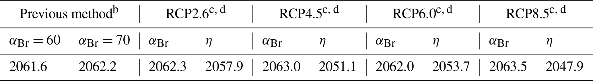
a Stratospheric mean age of air: 3 years. Fractional years provided to better demonstrate sensitivity of perturbation parameters. b EESC using static αBr calculated per Eq. (3). c Climate-variant EESC (column indicated by αBr) calculated per Eq. (5). d EESBnC (column indicated by η) calculated per Eq. (9) and benchmarked to Ξ=1980.
The propagation of EESC using climate-invariant αBr per Eq. (3) or climate-varying αBr per Eq. (5) produces significantly different dates of extrapolar halogen recovery than the propagation of EESBnC using η-factor normalization as in Eq. (9). EESC and EESBnC values are presented in Table 3 for historical and future chemistry–climate scenarios. In all cases, the computations were informed by the trend-independent fractional release factors provided in Table 1 of Engel et al. (2018a); though fractional release factors are likely to vary as the climate evolves (Leedham-Elvidge et al., 2018), these factors correlate with the specified dynamics employed in this analysis. The EESC and EESBnC calculations are visualized in Fig. 5.
In Fig. 5a, EESC is computed per Eq. (3) for static αBr = 60 (grey dashed line) and αBr = 70 (magenta dashed line) and per Eq. (5) using climate-varying αBr for the four RCP scenarios (colored solid lines). Values of αBr were interpolated between values indicated in Table 2. For reference, the black dots indicate 1980 EESC mixing ratios with αBr=70. Notably, there is very little variation between the RCP scenarios computed using Eq. (5), with a maximum deviation of 1.5 years (spanning January 2062–June 2063) for recovery to 1980 EESC values, as shown in Table 4. Scenarios of climate-invariant αBr=60 or αBr=70 provide EESC recovery dates (June 2061 and March 2062, respectively) in close agreement with the RCP scenarios. Note that for clarity, the 1980 EESC reference line for αBr=60 is not plotted in Fig. 5a.
Taking chemistry–climate changes into account (when Eq. (9) is used for EESBnC computation) results in significant variations in future EESBnC between the RCP scenarios, as shown in Fig. 5b. For comparison purposes, as in panel (a), the black dots provide the 1980 chemistry–climate benchmark EESC mixing ratio with αBr=70, and the dashed magenta line shows EESC propagated with climate-invariant αBr=70 (equivalently calculated here with ηCl=1 and ηBr=70). The range of values for the return of EESBnC to 1980 levels between the RCP scenarios in panel (b) spans a decade, 2048 to 2058, as shown in Table 4. For all RCP scenarios, the expected recovery date of the inorganic halogen content of the stratosphere to the ozone-depleting equivalent of the year 1980 is significantly sooner than the date expected using EESC. Importantly, the earlier ozone recovery dates predicted by EESBnC using Eq. (9) are in closer agreement with the 3-D CCM results of Dhomse et al. (2018) than recovery dates calculated using EESC. We note that this analysis does not include the impact of an accelerated Brewer–Dobson circulation, which would further hasten our projected date of recovery.
The divergences of expected values between the calculation techniques are even more pronounced as the century unfolds. Figure 5c provides the differences between EESC calculated with Eq. (5) and EESBnC calculated using Eq. (9). As the century ends, the EESBnC method shows that there is a difference exceeding 300 pptv of equivalent stratospheric Cl in the RCP8.5 scenario relative to a calculation of EESC. These discrepancies are negligible in the RCP2.6 scenario because the greenhouse gas inventory of the RCP2.6 year 2100 scenario is very similar to the greenhouse gas inventory of the contemporary stratosphere. Intermediate greenhouse gas scenarios lie between these two extremes.
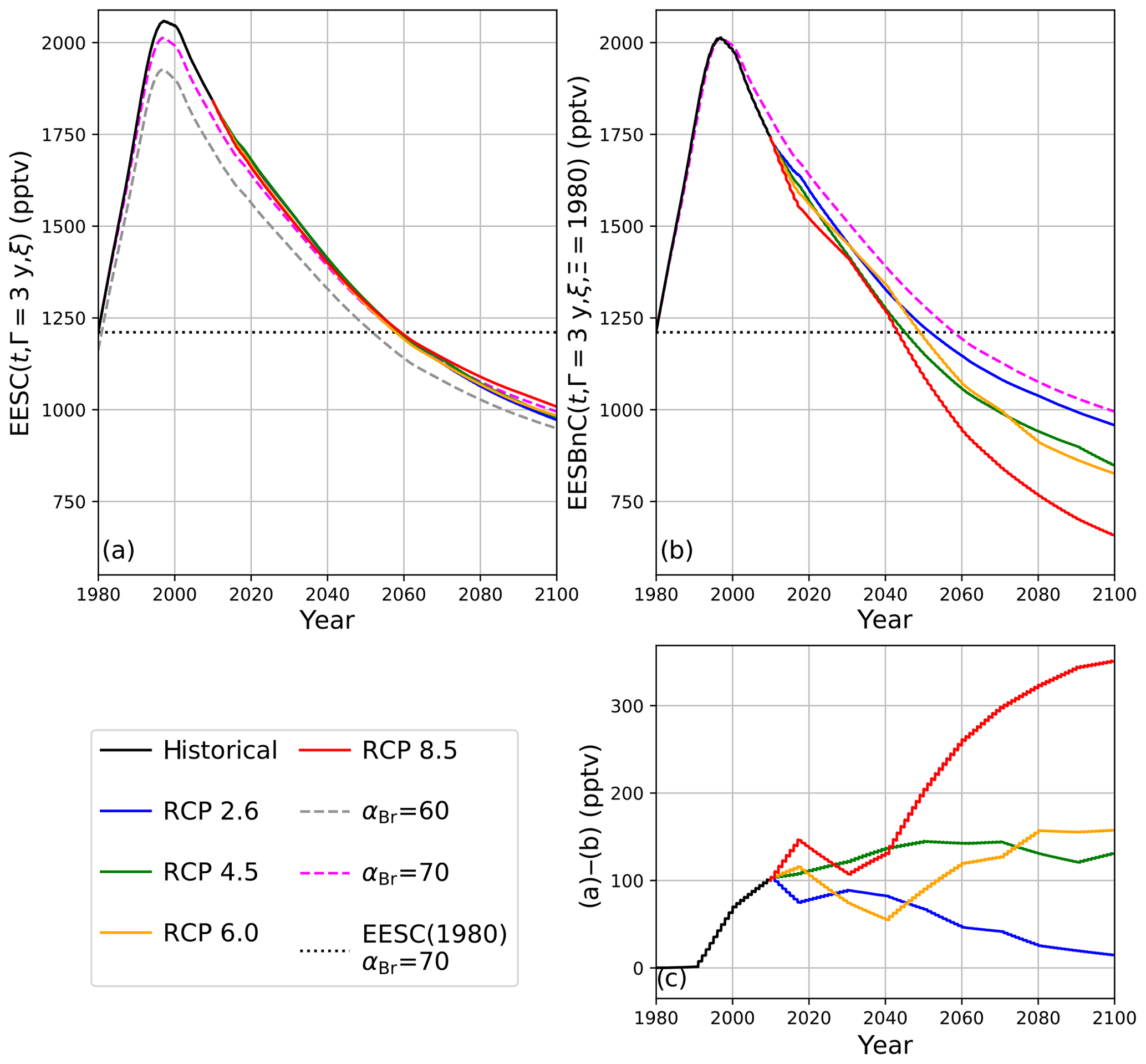
Figure 5Calculations of EESC and EESBnC for 1980–2100 using 3-year stratospheric mean age. (a) EESC calculated per Eqs. (3) and (5). Dashed traces: constant αBr as indicated in the legend. Solid traces: αBr interpolated as a function of time from values indicated in Table 2. Dotted black line: EESC corresponding to the year 1980 with αBr=70. (b) Calculation of EESBnC per Eq. (9) with benchmark chemistry–climate state Ξ=1980. Solid lines: ηCl and ηBr interpolated as a function of time from values indicated in Table 2. Magenta dashed line: EESBnC propagated with static ηCl=1 and ηBr=70 (equivalent to EESC calculated per Eq. (3) with αBr=70, as in a). Dotted black line: EESC corresponding to the year 1980 with αBr=70. (c) RCP scenario differences between (a) and (b).
The future stratosphere will be very different than the stratosphere of today in terms of trace gas loading, temperature structure, and radiative–dynamical transport. In this work, we used a 2-D chemical-transport–aerosol model to evaluate how differences in the trace gas loading and the temperature structure of the future atmosphere might influence the relative rates at which inorganic halogen species destroy ozone. These differences can be quite large and are very sensitive to the chemistry–climate boundary conditions imposed.
We provide the framework for adjusting EESC to accommodate changes in the ozone-processing rates of both chlorine and bromine driven by climate and chemistry. Current formulations of the bromine alpha factor obfuscate the fact that rates of ozone destruction by chlorine are changing alongside rates of ozone destruction by bromine. In some cases, as in RCP8.5, these rates change in concert, producing a largely time-invariant αBr over the course of the 21st century; however, the actual rates of ozone destruction facilitated by chlorine and bromine would have changed significantly, declining to about 65 % of their 1980 values. For this reason, we have refactored the bromine alpha factor in terms of a climate normalization using new eta factors, which provide an indication of the ozone-processing power of the atmosphere relative to a benchmark chemistry–climate state.
When we insert ηCl and ηBr into the formulation for the time propagation of EESC (Eq. 9), we obtain EESBnC. This metric teases out differences in the capability of the inorganic halogen background of the stratosphere to destroy ozone as a function of future chemistry–climate scenarios. Using this treatment, we find that the emission of large quantities of CH4 and N2O, as in the RCP8.5 emission scenario, decreases the ozone-processing power of the end-of-century future atmosphere by 36 % relative to what would be expected by calculating EESC (as in Eq. 5). Using EESBnC, the recovery of the stratospheric ozone layer to the thickness observed in 1980 is predicted to be 14 years earlier than the date obtained using EESC in the RCP8.5 scenario, bringing parameterized estimates of the extrapolar ozone recovery date into closer agreement with more costly 3-D CCM simulations.
Replication data for this work may be obtained from the Harvard Dataverse: https://doi.org/10.7910/DVN/EMKTTM (Klobas, 2020).
JEK and DMW developed the concept. JEK, DKW, RJS, and DMW designed the experiment. JEK and RJS were responsible for implementation and data reduction. All authors discussed the results and developed the paper.
The authors declare they have no conflict of interest.
We gratefully acknowledge funding support from the National Science Foundation and the National Aeronautics and Space Administration. J. Eric Klobas thanks Norton Allen, James Anderson, William Ball, Gabriel Chiodo, Janina Hansen, and Thomas Peter for helpful discussions of the work. For our use of RCP temperature fields, we acknowledge the World Climate Research Programme's Working Group on Coupled Modelling, which is responsible for CMIP, and we thank the Japan Agency for Marine-Earth Science and Technology, Atmosphere and Ocean Research Institute (University of Tokyo), as well as the National Institute for Environmental Studies.
This research has been supported by the National Science Foundation, Division of Atmospheric and Geospace Sciences (grant no. 1764171) and the National Aeronautics and Space Administration – Atmospheric Composition and Modeling Program (ACMAP) (grant no. 80NSSC19K0983).
This paper was edited by Jens-Uwe Grooß and reviewed by Andreas Engel and one anonymous referee.
Austin, J. and Wilson, R. J.: Ensemble simulations of the decline and recovery of stratospheric ozone, J. Geophys. Res.-Atmos., 111, D16314, https://doi.org/10.1029/2005JD006907, 2006. a
Banerjee, A., Maycock, A. C., Archibald, A. T., Abraham, N. L., Telford, P., Braesicke, P., and Pyle, J. A.: Drivers of changes in stratospheric and tropospheric ozone between year 2000 and 2100, Atmos. Chem. Phys., 16, 2727–2746, https://doi.org/10.5194/acp-16-2727-2016, 2016. a
Braesicke, P., Neu, J., Fioletov, V., Godin-Beekmann, S., Hubert, D., Petropavlovskikh, I., Shiotani, M., and Sinnhuber, B.-M.: Update on Global Ozone: Past, Present, and Future, chap. 3, in: Scientific Assessment of Ozone Depletion: 2018, Global Ozone Research and Monitoring Project – Report No. 58, World Meteorological Organization, Geneva, Switzerland, 2018. a
Brasseur, G. P., Granier, C., and Walters, S.: Future changes in stratospheric ozone and the role of heterogeneous chemistry, Nature, 348, 626–628, https://doi.org/10.1038/348626a0, 1990. a
Brune, W. H. and Anderson, J. G.: In situ observations of midlatitude stratospheric ClO and BrO, Geophys. Res. Lett., 13, 1391–1394, https://doi.org/10.1029/GL013i013p01391, 1986. a
Burkholder, J. B., Sander, S. P., Abbatt, J. P. D., Barker, J. R., Huie, R. E., Kolb, C. E., Kurylo, M. J., Orkin, V. L., Wilmouth, D. M., and Wine, P. H.: Chemical kinetics and photochemical data for use in atmospheric studies, evaluation no. 18, JPL Publication 15-10, Jet Propulsion Laboratory, Pasadena, 2015. a, b
Butchart, N., Scaife, A., Bourqui, M., De Grandpré, J., Hare, S., Kettleborough, J., Langematz, U., Manzini, E., Sassi, F., Shibata, K., Shindell, D., and Sigmond, M.: Simulations of anthropogenic change in the strength of the Brewer–Dobson circulation, Clim. Dynam., 27, 727–741, https://doi.org/10.1007/s00382-006-0162-4, 2006. a
Charlton-Perez, A. J., Hawkins, E., Eyring, V., Cionni, I., Bodeker, G. E., Kinnison, D. E., Akiyoshi, H., Frith, S. M., Garcia, R., Gettelman, A., Lamarque, J. F., Nakamura, T., Pawson, S., Yamashita, Y., Bekki, S., Braesicke, P., Chipperfield, M. P., Dhomse, S., Marchand, M., Mancini, E., Morgenstern, O., Pitari, G., Plummer, D., Pyle, J. A., Rozanov, E., Scinocca, J., Shibata, K., Shepherd, T. G., Tian, W., and Waugh, D. W.: The potential to narrow uncertainty in projections of stratospheric ozone over the 21st century, Atmos. Chem. Phys., 10, 9473–9486, https://doi.org/10.5194/acp-10-9473-2010, 2010. a
Chiodo, G., Polvani, L. M., Marsh, D. R., Stenke, A., Ball, W., Rozanov, E., Muthers, S., and Tsigaridis, K.: The response of the ozone layer to quadrupled CO2 concentrations, J. Clim., 31, 3893–3907, https://doi.org/10.1175/JCLI-D-17-0492.1, 2018. a
Chipperfield, M. and Pyle, J.: Model sensitivity studies of Arctic ozone depletion, J. Geophys. Res.-Atmos., 103, 28389–28403, https://doi.org/10.1029/98JD01960, 1998. a, b
Daniel, J. S., Solomon, S., and Albritton, D. L.: On the evaluation of halocarbon radiative forcing and global warming potentials, J. Geophys. Res.-Atmos., 100, 1271–1285, https://doi.org/10.1029/1999JD900381, 1995. a
Daniel, J. S., Solomon, S., Portmann, R., and Garcia, R.: Stratospheric ozone destruction: The importance of bromine relative to chlorine, J. Geophys. Res.-Atmos., 104, 23871–23880, https://doi.org/10.1029/1999JD900381, 1999. a, b, c
Danilin, M. Y., Sze, N.-D., Ko, M. K., Rodriguez, J. M., and Prather, M. J.: Bromine-chlorine coupling in the Antarctic Ozone Hole, Geophys. Res. Lett., 23, 153–156, https://doi.org/10.1029/95GL03783, 1996. a, b
Dhomse, S. S., Kinnison, D., Chipperfield, M. P., Salawitch, R. J., Cionni, I., Hegglin, M. I., Abraham, N. L., Akiyoshi, H., Archibald, A. T., Bednarz, E. M., Bekki, S., Braesicke, P., Butchart, N., Dameris, M., Deushi, M., Frith, S., Hardiman, S. C., Hassler, B., Horowitz, L. W., Hu, R.-M., Jöckel, P., Josse, B., Kirner, O., Kremser, S., Langematz, U., Lewis, J., Marchand, M., Lin, M., Mancini, E., Marécal, V., Michou, M., Morgenstern, O., O'Connor, F. M., Oman, L., Pitari, G., Plummer, D. A., Pyle, J. A., Revell, L. E., Rozanov, E., Schofield, R., Stenke, A., Stone, K., Sudo, K., Tilmes, S., Visioni, D., Yamashita, Y., and Zeng, G.: Estimates of ozone return dates from Chemistry-Climate Model Initiative simulations, Atmos. Chem. Phys., 18, 8409–8438, https://doi.org/10.5194/acp-18-8409-2018, 2018. a, b, c, d, e
Engel, A., Bönisch, H., Ostermöller, J., Chipperfield, M. P., Dhomse, S., and Jöckel, P.: A refined method for calculating equivalent effective stratospheric chlorine, Atmos. Chem. Phys., 18, 601–619, https://doi.org/10.5194/acp-18-601-2018, 2018a. a, b, c, d, e
Engel, A., Rigby, M., B, B. J., Fernandez, R. P., Froidevaux, L., D, H. B., Hossaini, R., Saito, T., Vollmer, M. K., and Yao, B.: Update on Ozone-Depleting Substances (ODS) and Other Gases of Interest to the Montreal Protocol, chap. 1, in: Scientific Assessment of Ozone Depletion: 2018, Global Ozone Research and Monitoring Project – Report No. 58, World Meteorological Organization, Geneva, Switzerland, 2018b. a, b, c
Eyring, V., Cionni, I., Bodeker, G. E., Charlton-Perez, A. J., Kinnison, D. E., Scinocca, J. F., Waugh, D. W., Akiyoshi, H., Bekki, S., Chipperfield, M. P., Dameris, M., Dhomse, S., Frith, S. M., Garny, H., Gettelman, A., Kubin, A., Langematz, U., Mancini, E., Marchand, M., Nakamura, T., Oman, L. D., Pawson, S., Pitari, G., Plummer, D. A., Rozanov, E., Shepherd, T. G., Shibata, K., Tian, W., Braesicke, P., Hardiman, S. C., Lamarque, J. F., Morgenstern, O., Pyle, J. A., Smale, D., and Yamashita, Y.: Multi-model assessment of stratospheric ozone return dates and ozone recovery in CCMVal-2 models, Atmos. Chem. Phys., 10, 9451–9472, https://doi.org/10.5194/acp-10-9451-2010, 2010. a
Eyring, V., Arblaster, J. M., Cionni, I., Sedláček, J., Perlwitz, J., Young, P. J., Bekki, S., Bergmann, D., Cameron-Smith, P., Collins, W. J., Faluvegi, G., Gottschaldt, K.-D., Horowitz, L. W., Kinnison, D. E., Lamarque, J.-F., Marsh, D. R., Saint-Martin, D., Sudo, K., Szopa, S., and Watanabe, S.: Long-term ozone changes and associated climate impacts in CMIP5 simulations, J. Geophys. Res.-Atmos., 118, 5029–5060, https://doi.org/10.1002/jgrd.50316, 2013. a, b, c
Fleming, E. L., Jackman, C. H., Stolarski, R. S., and Considine, D. B.: Simulation of stratospheric tracers using an improved empirically based two-dimensional model transport formulation, J. Geophys. Res.-Atmos., 104, 23911–23934, https://doi.org/10.1029/1999JD900332, 1999. a, b, c, d
Klobas, J. E.: Replication Data for: Reformulating the Bromine Alpha Factor and EESC: Evolution of Ozone Destruction Rates of Bromine and Chlorine in Future Climate Scenarios, https://doi.org/10.7910/DVN/EMKTTM, 2020. a
Ko, M. K., Sze, N. D., Scott, C., Rodríguez, J. M., Weisenstein, D. K., and Sander, S. P.: Ozone depletion potential of CH3Br, J. Geophys. Res.-Atmos., 103, 28187–28195, https://doi.org/10.1029/98JD02537, 1998. a
Koenig, T. K., Baidar, S., Campuzano-Jost, P., Cuevas, C. A., Dix, B., Fernandez, R. P., Guo, H., Hall, S. R., Kinnison, D., Nault, B. A., Ullmann, K., Jimenez, J. L., Saiz-Lopez, A., and Volkamer, R.: Quantitative detection of iodine in the stratosphere, P. Natl. Acad. Sci. USA, 50, 1860–1866, https://doi.org/10.1073/pnas.1916828117, 2020. a
Lary, D.: Catalytic destruction of stratospheric ozone, J. Geophys. Res.-Atmos., 102, 21515–21526, https://doi.org/10.1029/97JD00912, 1997. a
Leedham Elvidge, E., Bönisch, H., Brenninkmeijer, C. A. M., Engel, A., Fraser, P. J., Gallacher, E., Langenfelds, R., Mühle, J., Oram, D. E., Ray, E. A., Ridley, A. R., Röckmann, T., Sturges, W. T., Weiss, R. F., and Laube, J. C.: Evaluation of stratospheric age of air from CF4, C2F6, C3F8, CHF3, HFC-125, HFC-227ea and SF6; implications for the calculations of halocarbon lifetimes, fractional release factors and ozone depletion potentials, Atmos. Chem. Phys., 18, 3369–3385, https://doi.org/10.5194/acp-18-3369-2018, 2018. a
Li, F., Stolarski, R. S., and Newman, P. A.: Stratospheric ozone in the post-CFC era, Atmos. Chem. Phys., 9, 2207–2213, https://doi.org/10.5194/acp-9-2207-2009, 2009. a
McElroy, M. B., Salawitch, R. J., Wofsy, S. C., and Logan, J. A.: Reductions of Antarctic ozone due to synergistic interactions of chlorine and bromine, Nature, 321, 759–762, https://doi.org/10.1038/321759a0, 1986. a
Meinshausen, M., Smith, S. J., Calvin, K., Daniel, J. S., Kainuma, M., Lamarque, J.-F., Matsumoto, K., Montzka, S., Raper, S., Riahi, K., Thomson, A., Velders, G. J. M., and van Vuuren, D. P. P.: The RCP greenhouse gas concentrations and their extensions from 1765 to 2300, Climatic Change, 109, 213–241, https://doi.org/10.1007/s10584-011-0156-z, 2011. a, b, c, d, e
Newman, P. A., Nash, E. R., Kawa, S. R., Montzka, S. A., and Schauffler, S. M.: When will the Antarctic ozone hole recover?, Geophys. Res. Lett., 33, L12814, https://doi.org/10.1029/2005GL025232, 2006. a, b
Newman, P. A., Daniel, J. S., Waugh, D. W., and Nash, E. R.: A new formulation of equivalent effective stratospheric chlorine (EESC), Atmos. Chem. Phys., 7, 4537–4552, https://doi.org/10.5194/acp-7-4537-2007, 2007. a
Oman, L., Waugh, D., Kawa, S., Stolarski, R., Douglass, A., and Newman, P.: Mechanisms and feedback causing changes in upper stratospheric ozone in the 21st century, J. Geophys. Res.-Atmos., 115, D05303, https://doi.org/10.1029/2009JD012397, 2010. a
Ostermöller, J., Bönisch, H., Jöckel, P., and Engel, A.: A new time-independent formulation of fractional release, Atmos. Chem. Phys., 17, 3785–3797, https://doi.org/10.5194/acp-17-3785-2017, 2017. a
Plummer, D. A., Scinocca, J. F., Shepherd, T. G., Reader, M. C., and Jonsson, A. I.: Quantifying the contributions to stratospheric ozone changes from ozone depleting substances and greenhouse gases, Atmos. Chem. Phys., 10, 8803–8820, https://doi.org/10.5194/acp-10-8803-2010, 2010. a
Rosenfield, J. E., Douglass, A. R., and Considine, D. B.: The impact of increasing carbon dioxide on ozone recovery, J. Geophys. Res.-Atmos., 107, ACH–7, https://doi.org/10.1029/2001JD000824, 2002. a
Salawitch, R. J., Weisenstein, D. K., Kovalenko, L. J., Sioris, C. E., Wennberg, P. O., Chance, K., Ko, M. K., and McLinden, C. A.: Sensitivity of ozone to bromine in the lower stratosphere, Geophys. Res. Lett., 32, L05811, https://doi.org/10.1029/2004GL021504, 2005. a, b
Sander, S. P., Ravishankara, A. R., Golden, D. M., Kolb, C. E., Kurylo, M. J., Molina, M. J., Moortgat, G. K., Finlayson-Pitts, B. J., Wine, P. H., and Huie, R. E.: Chemical kinetics and photochemical data for use in atmospheric studies, evaluation no. 15, JPL Publication 06-2, Jet Propulsion Laboratory, Pasadena, 2006. a, b
Sinnhuber, B.-M., Sheode, N., Sinnhuber, M., Chipperfield, M. P., and Feng, W.: The contribution of anthropogenic bromine emissions to past stratospheric ozone trends: a modelling study, Atmos. Chem. Phys., 9, 2863–2871, https://doi.org/10.5194/acp-9-2863-2009, 2009. a, b, c
Solomon, S., Garcia, R. R., Rowland, F. S., and Wuebbles, D. J.: On the depletion of Antarctic ozone, Nature, 321, 755–758, https://doi.org/10.1038/321755a0, 1986. a
Solomon, S., Mills, M., Heidt, L., Pollock, W., and Tuck, A.: On the evaluation of ozone depletion potentials, J. Geophys. Res.-Atmos., 97, 825–842, https://doi.org/10.1029/94JD02028, 1992. a
Van Vuuren, D. P., Edmonds, J., Kainuma, M., Riahi, K., Thomson, A., Hibbard, K., Hurtt, G. C., Kram, T., Krey, V., Lamarque, J.-F., Masui, T., Meinshausen, M., Nakicenovic, N., Smith, S. J., and Rose, S. K.: The representative concentration pathways: an overview, Climatic Change, 109, 5–31, https://doi.org/10.1007/s10584-011-0148-z, 2011. a
Wales, P. A., Salawitch, R. J., Nicely, J. M., Anderson, D. C., Canty, T. P., Baidar, S., Dix, B., Koenig, T. K., Volkamer, R., Chen, D., Huey, G. L., Tanner, D. J., Cuevas, C. A., Fernandez, R. P., Kinnison, D. E., Lamarque, J.-F., Saiz-Lopez, A., Atlas, E. L., Hall, S. R., Navarro, M. A., Pan, L. L., Schauffler, S. M., Stell, M., Tilmes, S., Ullmann, K., Weinheimer, A. J., Akiyoshi, H., Chipperfield, M. P., Deushi, M., Dhomse, S. S., Feng, W., Graf, P., Hossaini, R., Jöckel, P., Mancini, E., Michou, M., Morgenstern, O., Oman, L. D., Pitari, G., Plummer, D. A., Revell, L. E., Rozanov, E., Saint-Martin, D., Schofield, R., Stenke, A., Stone, K. A., Visioni, D., Yamashita, Y., and Zeng, G.: Stratospheric injection of brominated very short-lived substances: Aircraft observations in the Western Pacific and representation in global models, J. Geophys. Res.-Atmos., 123, 5690–5719, https://doi.org/10.1029/2017JD027978, 2018. a
Watanabe, S., Hajima, T., Sudo, K., Nagashima, T., Takemura, T., Okajima, H., Nozawa, T., Kawase, H., Abe, M., Yokohata, T., Ise, T., Sato, H., Kato, E., Takata, K., Emori, S., and Kawamiya, M.: MIROC-ESM 2010: model description and basic results of CMIP5-20c3m experiments, Geosci. Model Dev., 4, 845–872, https://doi.org/10.5194/gmd-4-845-2011, 2011. a, b
Waugh, D., Oman, L., Kawa, S., Stolarski, R., Pawson, S., Douglass, A., Newman, P., and Nielsen, J.: Impacts of climate change on stratospheric ozone recovery, Geophys. Res. Lett., 36, https://doi.org/10.1029/2008GL036223, L03805, 2009. a
Weisenstein, D. K., Penner, J. E., Herzog, M., and Liu, X.: Global 2-D intercomparison of sectional and modal aerosol modules, Atmos. Chem. Phys., 7, 2339–2355, https://doi.org/10.5194/acp-7-2339-2007, 2007. a
Weisenstein, D. K., Yue, G. K., Ko, M. K., Sze, N.-D., Rodriguez, J. M., and Scott, C. J.: A two-dimensional model of sulfur species and aerosols, J. Geophys. Res.-Atmos., 102, 13019–13035, https://doi.org/10.1029/97JD00901, 1997. a
Wofsy, S. C., McElroy, M. B., and Yung, Y. L.: The chemistry of atmospheric bromine, Geophys. Res. Lett., 2, 215–218, https://doi.org/10.1029/GL002i006p00215, 1975. a
World Meteorological Organization: Scientific Assessment of Ozone Depletion: 2018, Global Ozone Research and Monitoring Project – Report No. 58, World Meteorological Organization, Geneva, Switzerland, 2018. a, b, c
Yung, Y., Pinto, J., Watson, R., and Sander, S.: Atmospheric bromine and ozone perturbations in the lower stratosphere, J. Atmos. Sci., 37, 339–353, https://doi.org/10.1175/1520-0469(1980)037<0339:ABAOPI>2.0.CO;2, 1980. a
Zubov, V., Rozanov, E., Egorova, T., Karol, I., and Schmutz, W.: Role of external factors in the evolution of the ozone layer and stratospheric circulation in 21st century, Atmos. Chem. Phys., 13, 4697–4706, https://doi.org/10.5194/acp-13-4697-2013, 2013. a