Temporal and spatial analysis of ozone concentrations in Europe based on timescale decomposition and a multi-clustering approach

Air quality measures that were implemented in Europe in the 1990s resulted in reductions of ozone precursor concentrations. In this study, the effect of these reductions on ozone is investigated by analyzing surface measurements of this pollutant for the time period between 2000 and 2015. Using a nonparametric timescale decomposition methodology, the long-term, seasonal and short-term variation in ozone observations were extracted. A clustering algorithm was applied to the different timescale variations, leading to a classification of sites across Europe based on the temporal characteristics of ozone. The clustering based on the long-term variation resulted in a site-type classification, while a regional classification was obtained based on the seasonal and short-term variations. Long-term trends of deseasonalized mean and meteo-adjusted peak ozone concentrations were calculated across large parts of Europe for the time period 2000–2015. A multidimensional scheme was used for a detailed trend analysis, based on the identified clusters, which reflect precursor emissions and meteorological influence either on the inter-annual or the short-term timescale. Decreasing mean ozone concentrations at rural sites and increasing or stabilizing at urban sites were observed. At the same time, downward trends for peak ozone concentrations were detected for all site types. In addition, a reduction of the amplitude in the seasonal cycle of ozone and a shift in the occurrence of the seasonal maximum towards earlier time of the year were observed. Finally, a reduced sensitivity of ozone to temperature was identified. It was concluded that long-term trends of mean and peak ozone concentrations are mostly controlled by precursor emissions changes, while seasonal cycle trends and changes in the sensitivity of ozone to temperature are among other factors driven by regional climatic conditions.

1 Introduction

Tropospheric ozone (O₃), together with particulate matter and nitrogen dioxide (NO₂), is one of the most troublesome air pollutants in Europe (EEA, 2016). A total of 17 000 premature deaths every year are attributed to excess O₃ exposure, without any sign of reduction in number of fatalities (EEA, 2016). In terms of impact on ecosystems, elevated concentrations of tropospheric O₃ are responsible for damaging agricultural production and forests mainly by reducing their growth rate. In addition, tropospheric O₃ acts as a greenhouse gas with an estimated globally averaged radiative forcing of 0.4±0.2 W m⁻² (IPCC, 2013). In the 1990s, emission control measures on O₃ precursors, namely nitrogen oxides (${\mathrm{NO}}_x=\mathrm{NO}+{\mathrm{NO}}_{\mathrm{2}}$) and volatile organic compounds (VOCs), were implemented in order to regulate air pollution. As a result, concentrations of NO_x and VOCs have significantly declined in Europe (EEA, 2017; Colette et al., 2011; Guerreiro et al., 2014; Henschel et al., 2015). NO_x emissions in particular declined in Europe by 48 % between 1990 and 2015 (EEA, 2017).

Surprisingly, O₃ concentrations have not decreased as expected (Oltmans et al., 2013; Colette et al., 2018). Mean O₃ concentrations either remained stable or even increased in rural background areas from the 1990s and even until the mid-2000s in many European countries (e.g., Boleti et al., 2018; Munir et al., 2013; Paoletti et al., 2014; Querol et al., 2016; Anttila and Tuovinen, 2009). At urban sites an increase in mean O₃ has been observed; in some cases, an increase has been found at both rural and urban sites with larger upward trends observed at urban compared to the rural sites (Paoletti et al., 2014; Querol et al., 2016; Anttila and Tuovinen, 2009). However, a change in the trend has been observed after the mid-2000s, when mean O₃ concentrations have started to decline (Boleti et al., 2018; Munir et al., 2013). On the other hand, maximum O₃ concentrations decreased continuously from the 1990s until present (Paoletti et al., 2014), except for the traffic-loaded environments (Boleti et al., 2019). Downward trends of different metrics for peak O₃ have been found at many sites across Europe (Fleming et al., 2018). However, the high year-to-year variability of O₃ tends to mask the long-term changes, leading to a large fraction of sites with nonsignificant trends. Several studies based on either observations or climate models have shown that anthropogenic emissions can affect O₃ concentrations across continents (Dentener et al., 2010; Wild and Akimoto, 2001; Lin et al., 2017). The increase in background O₃ in Europe has been associated with increasing stratospheric O₃ contribution (Ordóñez et al., 2007), as well as increased hemispheric transport of O₃ and its precursors.

A shift in the seasonal cycle of O₃ has been observed in northern midlatitudes, i.e., the peak concentrations are now observed earlier in the year compared to previous decades, with a rate of 3–6 d per decade. (Parrish et al., 2013). This shift is attributed to increasing emissions of O₃ precursors in developing countries that led to an equatorward redistribution of precursors in previous decades (Zhang et al., 2016). Negative trends of the 95th percentile of O₃ and positive trends for the 5th percentile have been detected across Europe (Yan et al., 2018). Simultaneous decrease in maximum concentrations in summer and increase in winter indicate a decrease in amplitude in the seasonal variation in O₃, probably as a result of the regulations in the 1990s (Simon et al., 2015).

O₃ variations are largely governed by climate and weather variability (Yan et al., 2018). Temperature especially influences O₃ concentrations in the troposphere, mainly by increasing the rates of several chemical reactions and increasing emissions of biogenic VOCs with increasing temperature (Sillman and Samson, 1995). Thermal decomposition of peroxyacyl nitrates (PANs) at high air temperature conditions results in elevated O₃ concentrations (Dawson et al., 2007). Indeed, extreme O₃ concentrations in central Europe are mainly associated with high temperatures (Otero et al., 2016). However, there are indications that the relationship of O₃ to temperature has changed in the last 20 years. For instance, in the US, O₃ climate penalty – defined as the slope of the O₃ versus temperature relationship – dropped from 3.2 ppbv ^∘C⁻¹ before 2002 to 2.2 ppbv ^∘C⁻¹ after 2002 as a result of NO_x emission reductions (Bloomer et al., 2009). Additionally, Colette et al. (2015), based on chemistry–transport and climate–chemistry model projections, assessed the impact of climate change on the climate penalty and found that over European land surfaces summer O₃ change is [0.44; 0.64] and [0.99; 1.50] ppbv (95 % confidence interval) for the 2041–2070 and 2071–2100 time periods, respectively.

At different locations, O₃ may show a different temporal evolution due to a variety of factors, such as local pollution, topography, influence of nearby sources, or even trans-boundary transport of O₃ and its precursors. In addition, meteorological conditions can vary amongst different locations within large regions such as Europe, affecting O₃ concentrations in various ways. O₃ trend studies in the past have tried to tackle this issue, mainly by using clustering techniques to categorize European measurement sites based on different O₃ metrics (e.g., Henne et al., 2010). For instance, a site-type classification representing O₃ regimes between 2007 and 2010 was obtained by Lyapina et al. (2016) using mean seasonal and diurnal variations. In addition, a geographical categorization reflecting the synoptic meteorological influence on O₃ variation between 1998 and 2012 was obtained by Carro-Calvo et al. (2017). To tackle low spatial representation of urban and rural sites across large domains, i.e., midlatitude North America, western Europe and East Asia, Chang et al. (2017) obtained a latitude-dependent site classification with lower concentrations in western and northern Europe and higher concentrations in southern Europe. These studies indicate that the selected metric used to characterize O₃ in clustering leads to site classifications that represent different aspects of O₃ variability.

In the current study, a multidimensional clustering method that captures several influencing factors for the long-term trend of O₃ is presented. The temporal and spatial evolution of O₃ concentrations between 2000 and 2015 is studied using data provided by the European Environmental Agency (EEA). Mean O₃ concentrations are decomposed into the underlying frequencies based on a nonparametric timescale decomposition method to obtain the long-term (LT), seasonal (S) and short-term (W) variations. The multidimensional clustering approach is applied to the distinct frequency signals LT(t) and S(t) extracted from the observations.

In addition, long-term trends of deseasonalized daily mean O₃ and meteo-adjusted peak O₃ concentrations are calculated. Through deseasonalization and meteo-adjustment, a significant fraction of the meteorologically driven variability of O₃ is excluded from the observations, and uncertainty in the trend estimation is reduced by a large factor. Intersections of site groups, i.e., LT(t) and S(t) clusters, are employed to guide the study of O₃ long-term trends. Furthermore, changes in the amplitude and phase of the seasonal variability of O₃ are explored based on the S(t) signal obtained by the timescale decomposition methodology. Finally, long-term changes in the relationship between O₃ and temperature are estimated and discussed for the different site environments and regions in Europe.

2 Data

Data for O₃ surface measurements are provided by the EEA (Air Quality e-Reporting) in an hourly resolution for the period between 2000 and 2015. In this study, only time series with a maximum of 15 % of missing values and a maximum of 120 consecutive days with missing values are used for the whole period of measurements, leaving the study with 291 sites across the European domain (Fig. 1). The daily mean and the daily maximum of the 8 h running mean based on hourly mean concentrations (MDA8 O₃) are calculated following the definition by the European Union Directive of 2008 (European Parliament and Council of the European Union, 2008). For the representation of peak concentrations the following metrics are used: (a) MTDM, which is the mean of the 10 highest daily maximum O₃ concentrations between May and September based on hourly mean data, and (b) 4-MDA8, the mean of the 4 highest MDA8 O₃ concentrations per year.

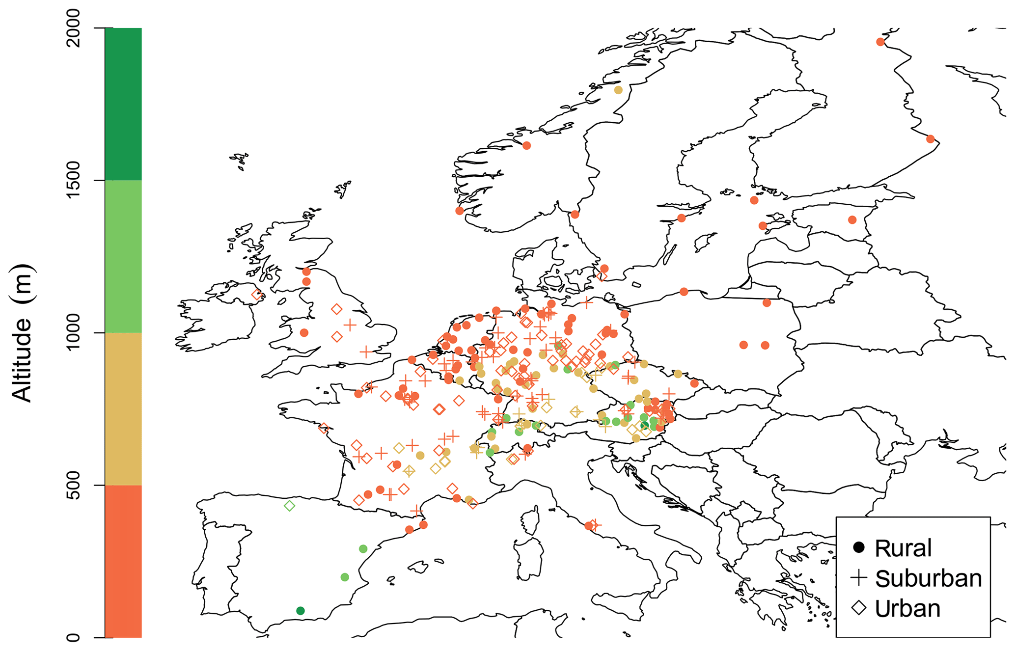
Figure 1 Map of Europe showing the location of the studied sites. Types of environment (symbols) and altitude (color bar) are indicated.

Meteorological variables are extracted from the ERA-Interim dataset on a 1^∘ grid at the location (longitude–latitude–altitude) of each station and in 3-hourly intervals. The variables considered for the meteo-adjustment of the peak O₃ metrics are temperature (K), specific humidity (g kg⁻¹), surface pressure (hPa), boundary layer height (m), convective available potential energy (CAPE, J kg⁻¹), east–west surface stress (N s m²) and north–south surface stress (N s m²).

The present trend analysis focuses on (a) the deseasonalized daily mean and MDA8 O₃ and (b) the meteo-adjusted MTDM and 4-MDA8 concentrations. The analysis of changes in the seasonal cycle of O₃ across Europe is based on the daily mean O₃ concentrations.

3 Methods

3.1 Timescale decomposition of daily mean and MDA8 O₃

Timescale decomposition refers to decomposition of the O₃ time series into the relevant underlying frequencies:

$$\begin{array}{}\text{(1)}& {\mathrm{O}}_{\mathrm{3}}\left(t\right)=\mathit{LT}\left(t\right)+S\left(t\right)+W\left(t\right)+E\left(t\right),\end{array}$$

where O₃(t) is the daily mean and MDA8 O₃ time series, LT(t) the long-term variation, S(t) the seasonal variation, W(t) the short-term variation, and E(t) the remainder of the decomposition. Timescale decomposition in this study is performed with a nonparametric method, called the ensemble empirical mode decomposition (EEMD, Huang et al., 1998; Huang and Wu, 2008; Wu and Huang, 2009), which is considered a powerful method for decomposing O₃ time series (Boleti et al., 2018). The method detects the hidden frequencies in the time series based merely on the data and yields the so-called intrinsic mode functions (IMFs); each IMF represents one distinct frequency in the signal:

$$\begin{array}{}\text{(2)}& y\left(t\right)=\sum _{j=\mathrm{1}}^n{c}_j\left(t\right)+\mathit{LT}\left(t\right),\end{array}$$

where y(t) is the input data, c_j is the different IMFs, n is the number of the IMFs and the remainder of the time series is the LT(t) of the input data. By adding together the IMFs with frequencies between around 40 d and 3 years we obtain the seasonal variation in O₃ ($S\left(t\right)=c_{\mathrm{7}}\left(t\right)+\mathrm{\dots }+c_{\mathrm{10}}\left(t\right)$), and by adding the frequencies that are smaller than 40 d the short-term variation is acquired ($W\left(t\right)=c_{\mathrm{1}}\left(t\right)+\mathrm{\dots }+c_{\mathrm{6}}\left(t\right)$). A more detailed discussion on the choice of the IMFs for the seasonal and short-term variations can be found in the study by Boleti et al. (2018).

3.2 Cluster analysis of O₃ variations

Cluster analysis is referred to pattern recognition in high-dimensional data. The main idea is to represent n objects by identifying k groups based on levels of similarity. Objects in the same group must have the highest level of similarity, while objects from different groups must have a low level of similarity (Jain, 2010). The partitioning around medoids (PAM) clustering algorithm is used in this study. It is based on k means (MacQueen, 1967; Hartigan and Wong, 1979), which is a widely used clustering technique (e.g., Lyapina et al., 2016). PAM is more robust than k means and less sensitive to outliers because it uses medoids (actual points in the data) instead of centroids (usually artificial points) (R Development Core Team, 2017). It works as follows: first, a set of n high-dimensional objects (measurement sites) is clustered into a set of k clusters. Initially, k clusters are generated randomly, and the empirical means m_k of the Euclidean distance between their data points are calculated. Then, each data point is assigned to its nearest cluster center (centroid). Centroids are iteratively updated by taking the medoid of all data points assigned to their clusters. The squared error (ε) between the m_k and the points in the cluster (x_i) is calculated as follows:

$$\begin{array}{}\text{(3)}& \mathit{\epsilon }=\sum _{i=\mathrm{1}}^n{∥x_i-m_k∥}^{\mathrm{2}}.\end{array}$$

Each centroid defines one of the clusters and each data point is assigned to its nearest centroid, and the iterative process is terminated when the ϵ is minimized.

For identification of the clusters, the LT(t), S(t) and W(t) of the daily mean and MDA8 O₃ were used as input time series in the PAM algorithm. A sufficient number of clusters must be defined in order to capture dominant behaviors such that redundant information is avoided but at the same time not overlooking important characteristics. To identify the optimal number of clusters, the PAM algorithm is iteratively executed for a range of k values (number of clusters) and the average sum of ϵ (SSE) is calculated for each iteration, i.e., each k.

$$\begin{array}{}\text{(4)}& \mathrm{SSE}=\sum _{i=\mathrm{1}}^n{\mathit{\epsilon }}^{\mathrm{2}}\end{array}$$

The number of clusters with the largest reduction in SSE is considered the most representative. Eventually, the choice of the ideal number of clusters results from a combination of the SSE approach and interpretability of the obtained clusters. In addition, a silhouette width (S_w) analysis is performed to assess the goodness of the clustering (Rousseeuw, 1987).

More details about the number of clusters, the goodness of the clustering and the S_w are provided in the Supplement (Sects. S1 and S2).

3.3 Daily mean and MDA8 O₃ long-term trend analysis

Meteorological adjustment is essential for calculation of robust O₃ long-term trends. Thus, daily mean and MDA8 O₃ observations are deseasonalized by subtracting the S(t) obtained with the EEMD from the observations (Boleti et al., 2018):

$$\begin{array}{}\text{(5)}& y_{\mathrm{d}}\left(t\right)=y\left(t\right)-S\left(t\right),\end{array}$$

where y_d(t) is the deseasonalized time series and y(t) the observations. Through deseasonalization, observations are adjusted for the effect of meteorology on the inter-annual timescale. Theil–Sen trends (Theil, 1950; Sen, 1968) are then calculated based on monthly mean deseasonalized concentrations y_d(t) for the period 2000–2015. The 95 % confidence interval of the trend is obtained by bootstrapping. The Theil–Sen trends were estimated using the openair library in R (R Development Core Team, 2017).

3.4 Peak O₃ concentrations long-term trend analysis

Trend analysis of peak O₃ metrics is performed for the MTDM and the 4-MDA8 O₃, based on a meteo-adjustment approach following Boleti et al. (2019). A different approach for meteorological adjustment was used for the peak O₃ than for the daily mean and MDA8; deseasonalization is not meaningful for peak O₃ because peak O₃ events are temporally localized. Thus, daily maximum and MDA8 O₃ observations were linked to the available meteorological variables through generalized additive models (GAMs, Hastie and Tibshirani, 1990; Wood, 2006). The models are fitted for the warm season May–September, as by definition the MTDM refers to this period of the year. GAMs are instances of generalized linear models in which the model is specified as a sum of smooth functions of the covariates. A GAM can be described as follows:

$$\begin{array}{}\text{(6)}& {\mathrm{O}}_{\mathrm{3}}\left(t\right)=\mathit{\alpha }+\sum _{i=\mathrm{1}}^n{s}_i\left(M_i\left(t\right)\right)+s_{\mathrm{0}}\left(t\right)+\mathit{ϵ}\left(t\right),\end{array}$$

where O₃(t) stands for the O₃ time series observations (daily maximum and MDA8), α is the intercept, s_i is the smooth functions (thin plates splines) of the numeric meteorological variables M_i and n denotes the number of the numeric meteorological variables in the GAM. The temporal trend is represented through the smooth function s₀(t), where t is the time variable expressed by the Julian day. Finally, ϵ stands for the residuals of the model. For the GAMs, the following meteorological variables were used: the daily maximum temperature, daily mean specific humidity, daily mean surface pressure, daily maximum boundary layer height, morning mean CAPE, daily mean east–west surface stress and daily mean north–south surface stress, as well as a time variable, i.e., the Julian day. The above explanatory meteorological variables are the ones that were most often selected at the Swiss sites by the meteorological variable selection performed by Boleti et al. (2019). The GAMs were estimated with the mgcv library in R (R Development Core Team, 2017).

The meteo-adjusted daily maximum and MDA8 O₃ concentrations were calculated similar to the approach applied by Barmpadimos et al. (2011):

$$\begin{array}{}\text{(7)}& {\mathrm{O}}_{{\mathrm{3}}_{\mathrm{metadj}}}\left(t\right)=\mathit{\alpha }+s_{\mathrm{0}}\left(t\right)+\mathit{ϵ}\left(t\right),\end{array}$$

where α is the intercept of the model, s₀(t) the time variable as Julian day and ϵ(t) the residuals. The meteo-adjusted MTDM and 4-MDA8 concentrations were estimated based on the meteo-adjusted values (${\mathrm{O}}_{{\mathrm{3}}_{\mathrm{adj}}}\left(t\right)$) on the same days as they were identified before the meteo-adjustment. Eventually, meteo-adjusted trends were calculated with the Theil–Sen trend estimator applied on the ${\mathrm{O}}_{{\mathrm{3}}_{\mathrm{metadj}}}\left(t\right)$.

3.5 O₃ seasonal cycle trend analysis

The S(t) signal extracted with the EEMD captures the meteorologically driven O₃ variation on yearly to multiyear timescales and is more representative compared to parametric fitting approaches (Boleti et al., 2018). Here, changes in the daily mean S(t) of O₃ throughout the studied period are identified as follows: the maximum and minimum O₃ value, as well as the day when the maximum O₃ occurred in each year, are identified in the S(t), referred to here as S_max, S_min and S_DoM, respectively (Fig. 2). A Theil–Sen trend estimator for each of the S_max(t), S_min(t) and S_DoM(t) is applied for each site cluster, representing the long-term temporal evolution of the amplitude and phase of S(t).

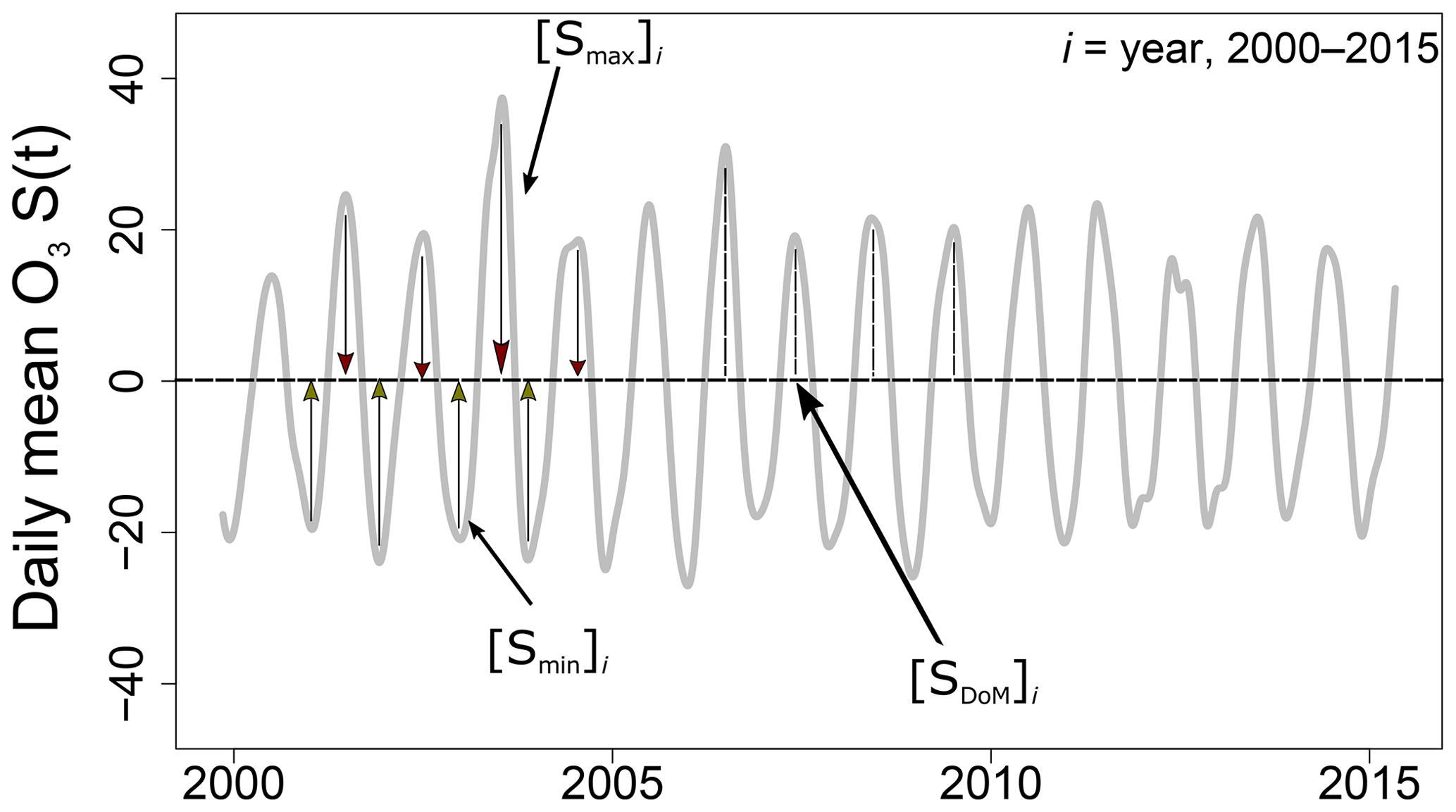
Figure 2 Schematic illustration for explaining the estimation of the (S_max(t) and S_min(t)) and the annual day of maximum of the seasonal signal (S_DoM(t)) as calculated from the daily mean O₃ time series.

3.6 Relationship between O₃ and temperature

The relationship between O₃ and temperature is studied for the warm season between May and September. A linear regression model between daily maximum O₃ concentrations and daily maximum temperature is applied for each year throughout the studied period 2000–2015 as follows:

$$\begin{array}{}\text{(8)}& {\mathrm{O}}_{\mathrm{3}}(t{)}_i={\mathit{\beta }}_{\mathrm{0}i}+{\mathit{\beta }}_{\mathrm{1}i}\cdot T(t{)}_i,i=\mathrm{1},\mathrm{2},\mathrm{\dots }n,\end{array}$$

where O₃(t) is the time series of the daily maximum O₃, T(t) the time series of the daily maximum temperature and n is the number of years. β_0i is the intercept and β_1i(t) the parameter describing the linear effect of temperature on O₃. Then, a linear model is applied to β_1i(t) over all years for each site cluster to identify the long-term trend of the slope between O₃ and temperature maximum values. In addition, a linear regression model is applied on the daily maximum O₃ concentrations against binned temperature ranges and in three consequent time periods (2000–2005, 2005–2010 and 2010–2015).

4 Results

4.1 Cluster analysis

Here, we present the results of the daily mean LT(t) and S(t) clustering; results for the W(t) clustering and the cluster analysis based on the MDA8 are provided in the Supplement (Sect. S3). The clusters based on daily mean and MDA8 O₃ are rather similar; thus, the choice of clusters based on these two metrics does not affect the conclusions. The daily mean O₃ clusters depict the main influencing factors for O₃ trends, i.e., proximity to emission sources and meteorological conditions. Therefore, it is appropriate to study long-term trends based on the O₃ daily mean clusters. Application of the clustering algorithm to the LT(t) leads to a site-type classification, which largely reflects the proximity to emission sources of O₃ precursors. S(t) and W(t) clustering leads to a regional site classification, which reflects the importance of the climate on the annual cycle of O₃. It is observed that a few sites have a negative S_w, which means that these sites are assigned to a certain cluster, although they do not really fit into any of the identified clusters (see Supplement, Sects. S2 an S5). Nevertheless, the sites with negative S_w were not excluded from the data analysis as they do not have a noticeable influence on the results.

O₃ concentrations often increase with distance from emission sources of NO_x. Thus, LT(t) clustering leads to identification of site groups with similar types of environment in terms of proximity to precursor emissions and mean O₃ concentrations, which are indicative of multiannual changes in the O₃ time series (Boleti et al., 2018). This measurement-based classification can be more informative than reported station types, for example, there are rural sites with nearby pollution sources or even sites with surroundings that might have changed dramatically with time. In the following section, clusters obtained from analysis of daily mean O₃ are presented and discussed in detail; the clusters derived from MDA8 O₃ are similar and presented in the Supplement (Sect. S3).

Cluster analysis of the long-term variation LT(t) resulted in four clusters that mainly differ in the daily mean O₃ concentration levels: cluster 1 includes sites that are marked in the Air Quality e-Reporting data repository as being of rural site type and sites that are mostly located at relatively high altitudes (on average 800 to 1200 m). The sites in cluster 1 show the highest O₃ concentrations, as illustrated in Fig. 3. The high mean O₃ concentrations indicate that the sites in cluster 1 represent background situations with minor influence from nearby emissions of man-made O₃ precursors. This cluster is therefore denoted as background cluster (BAC). Cluster 2 includes mostly rural sites that are located at lower altitudes of around 300–600 m and is therefore labeled as rural cluster (RUR, Fig. 3). The sites in cluster 3 are also located at low altitudes (around 100 to 300 m) and represent rural, suburban and urban site types in similar numbers. The sites in cluster 3 seem to be influenced by nearby man-made emissions of O₃ precursors such as NO_x, leading to lower mean O₃ concentrations compared to the sites in the RUR cluster. Cluster 3 consists of moderately polluted sites and is denoted as cluster MOD. Finally, cluster 4 consists mostly of urban and suburban sites showing the lowest daily mean O₃ concentrations, likely due to the proximity to sources of NO_x emissions and the resulting enhanced depletion of O₃ through reaction with NO. Consequently, cluster 4 is denoted as the highly polluted cluster (HIG).

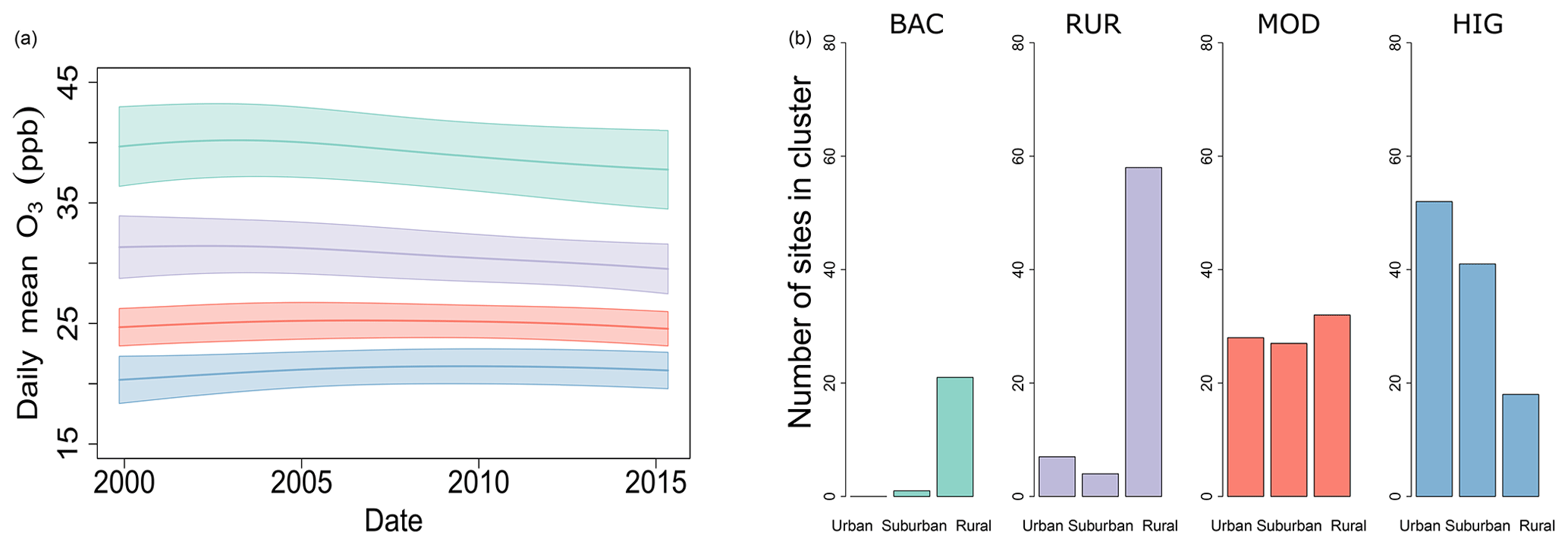
Figure 3 Clusters based on daily mean O₃ LT(t). Average LT(t) in each cluster with the standard deviation (a) and histograms (b) for the site type included in each cluster.

The LT(t) signal, as derived from the daily mean (Fig. 3) and MDA8 O₃ (Fig. S9 in the Supplement) observations, increases for BAC and RUR until around the beginning of the 2000s and decreases afterwards. For the MOD and HIG clusters the same pattern was observed, but the decrease starts much later than at the rural sites, i.e., around the end of the 2000s. Especially at the HIG sites a level-off is mostly observed after 2010 rather than a decrease. Similar temporal evolution with inflection points in the LT(t) has been observed in the study by Boleti et al. (2018) which was focused on trends of average O₃ concentrations in Switzerland.

Figure 4 Map with the site clusters derived from daily O₃ S(t) and average S(t) in each site cluster.

Clusters derived from the daily mean S(t) show a regional representation most likely due to the influence of the regional climate conditions and the annual cycle of O₃. The following five clusters were obtained from the daily mean S(t) (Fig. 4):

1. “CentralNorth” comprised of the northern and eastern parts of Germany; the Netherlands; and some eastern sites in Czech Republic, Poland, and Austria;

2. “CentralSouth” covers most of Austria, Switzerland, and some sites in southwestern Germany;

3. “West” incorporates the majority of France, Belgium, and Spain;

4. “PoValley” includes the sites located in the Po Valley, an industrial region in Northern Italy;

5. “North” covers most of the UK and Scandinavia.

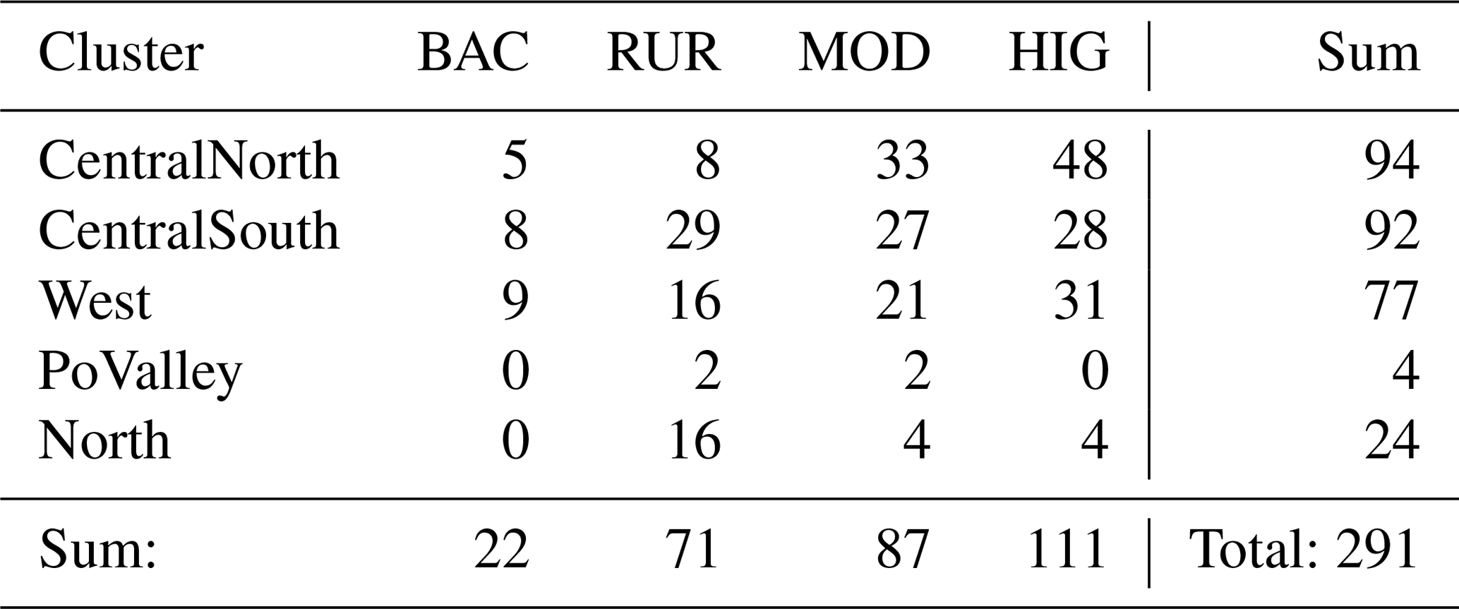
The number of sites included in each cluster are shown in Table 1. The sites in the PoValley cluster display the most pronounced S(t), mainly due to the Mediterranean weather conditions, e.g., high temperatures. At the same time, high NO_x and VOC emissions in this region leads to higher O₃ concentrations. Special topographic conditions (valley south of Alps) in combination with cyclonic systems lead to containment of emissions from the Milan industrial area in the PoValley cluster (Bärtsch-Ritter et al., 2004; Henne et al., 2005; Prévôt et al., 1997; Thunis et al., 2009). The North cluster has the smallest seasonal variability, due to generally low O₃ concentrations and lower temperature conditions in this region. At the Scandinavian sites in particular, meteorological conditions are rather unfavorable for O₃ formation. Also, the regions included in the North cluster are influenced by cyclonic systems arriving in Europe through the North Atlantic Ocean that carry air pollutants into Europe (Stohl, 2002; Dentener et al., 2010). Thus, the influence of background O₃, i.e., O₃ inflow from North America and East Asia, is high at these sites (Derwent et al., 2004, 2013). In all clusters (except in the North cluster) the hot summers of 2003 and 2006 are visible in the S(t) signal, which shows that the S(t) signal can capture important events in O₃ variability that are driven by seasonal meteorological phenomena. It is interesting to note that both CentralNorth sites have seasonal values in their signal comparable to the PoValley cluster values, probably related to industrial and agricultural emissions in the area of northern Germany.

Table 1 Number of sites in each site group based on the LT(t) and S(t) clusters.

A two-dimensional classification scheme is achieved by employing the LT(t) and S(t) clusters. Our results are in good agreement with previous classification studies, where by using different O₃ metrics similar classifications have been obtained. For instance, the spatial analysis based on gridded O₃ data (MDA8) across Europe by Carro-Calvo et al. (2017) resulted in a regional site classification. The gridded data used by Carro-Calvo et al. (2017) were obtained by spatial interpolation, leading to a larger and regular geographical coverage compared to the available observations. Compared to Carro-Calvo et al. (2017), similar geographical clusters were identified here, except for the Iberian Peninsula, eastern Europe, northern Scandinavia and the Balkan states that do not appear as separate clusters in our analysis. This is most probably due to the small number of observational sites in the above regions. In contrast to our study, gridded MDA8 O₃ concentrations during summer have exclusively been used for the cluster analysis by Carro-Calvo et al. (2017), and therefore in conditions wherein the correlation of O₃ and meteorological variables such as temperature is typically strongest. In addition, the present study results in spatial classification by utilizing the seasonal variation, while Carro-Calvo et al. (2017) have used normalized anomalies. Four site-type clusters were found based on the LT(t) in this study similar to Lyapina et al. (2016) based on absolute mixing ratios of O₃ variations, which identified five site-type clusters ranging from urban traffic (as in the HIG cluster here) to rural background environments (equivalent to RUR). Similar site classifications are obtained because the LT(t) signal of this study and the mean seasonal and diurnal profiles of Lyapina et al. (2016) both capture the O₃ concentration levels, distinguishing specific pollution regimes.

4.2 Trends of daily mean O₃ concentrations

The daily mean LT(t) and S(t) clusters identified in Sect. 4.1 are used for assessment of the temporal trends for the different site types and geographical locations. Overall, decreasing daily O₃ means are found for rural sites, while there is a tendency for increasing O₃ in more polluted urban environments (Fig. 5). MDA8 trends are similar to the daily mean trends and are shown in Sect. S4. At 64 % of all sites significant trends (p value < 0.05) were identified for the daily mean O₃; 61 % of the significant trends were negative and 39 % positive. Most rural sites – BAC and RUR – experienced decreasing daily mean O₃ concentrations in all regions, as expected following the NO_x and VOC reductions in Europe (Fig. 5). At the MOD and HIG sites a leveling off or increase is observed, respectively, especially in the CentralNorth, West and North clusters. At the HIG sites the positive trends could partly be explained by the increase in NO₂ to NO_x ratio, originating from the proliferation of diesel vehicles, which have increased in the European car fleet (EEA, 2009). In addition, the strong reduction of NO_x concentrations that led to less titration of O₃ by NO could also explain the positive trends at urban and suburban sites. The late inflection point at urban sites (LT(t) of HIG cluster in Fig. 3) could be an additional effect of the reduced titration of O₃, which leads to positive trends at the HIG sites. Flat trends at central European sites might partially be explained by the increasing influence of North American and Asian emissions, which have counterbalanced the decrease in European NO_x and VOC concentrations (Derwent et al., 2018; Yan et al., 2018).

Figure 5 Box plots of deseasonalized daily mean O₃ trends for the LT(t) and S(t) clusters. LT(t) clusters represent a site-type classification, while the S(t) clusters represent a geographical classification that is influenced by regional climate conditions. Boxes include 25th to 75th percentiles with the line indicating the median value; whiskers extend to 1.5 times the interquartile range.

In agreement with our results, significant decreases in daytime average and summertime mean of MDA8 O₃ at European rural sites, as well as small and nonsignificant downward trends of MDA8 at urban sites, have been found previously for the time period 2000–2014 (Chang et al., 2017). Similarly, in a report by EEA (2016) it was found that between 2000 and 2014 annual mean O₃ and annual mean MDA8 O₃ have been decreasing at rural background sites, while at more polluted sites influenced by nearby man-made precursor emissions upward trends have been detected.

O₃ trends at sites in the North cluster indicate changes in background O₃, especially in the RUR clusters that are mostly free from local emissions. Here, decreasing trends of daily mean O₃ were found at RUR sites, while in the MOD and HIG the trends are slightly increasing. It is interesting to compare the trends in the North cluster with the temporal evolution of O₃ at Mace Head (a remote station in northwestern Ireland), which is representative for inflow of background O₃ into Europe. For this reason, we estimated the LT(t) variation in MDA8 O₃ and the Theil–Sen trend for the site at Mace Head (Fig. 6) to compare with the MDA8 O₃ trend identified by Derwent et al. (2018). Here, an inflection point was identified in the LT(t) in 2006, i.e., MDA8 O₃ has been increasing between 1988 and 2006 and started to slightly decline after 2006. Deseasonalized Theil–Sen trends were estimated to be 0.08 ppb yr⁻¹ [0.06, 0.1] for the first period and −0.04 ppb yr⁻¹ [−0.09, 0.02] for the second period. Similarly, Derwent et al. (2018) have found an increase of 0.34±0.07 ppb yr⁻¹ with a deceleration rate after 2007 of $-\mathrm{0.0225}\pm \mathrm{0.008}$ ppb yr⁻² at the same station, based on a combination of filtered measurement data and modeling output (Lagrangian dispersion). The inflection point in the mid-2000s might be the reason for the flat trend of the annual average O₃ during 2000s as estimated by Derwent et al. (2013).

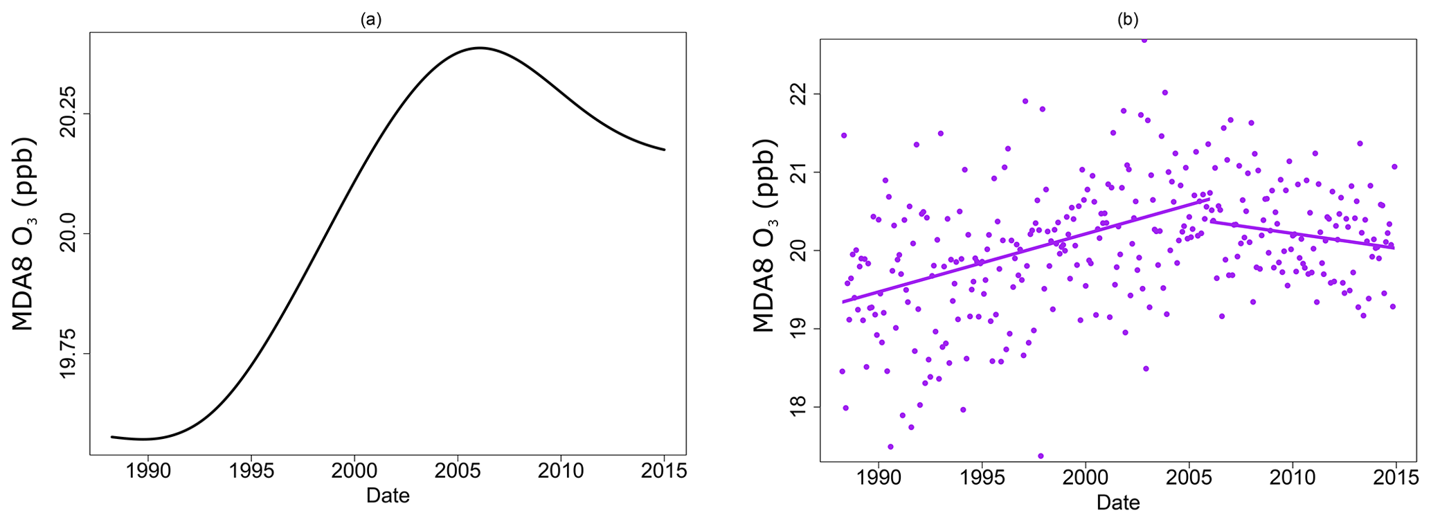
Figure 6 MDA8 LT(t) at Mace Head extracted with the EEMD (a) and the corresponding deseasonalized Theil–Sen trend (b).

4.3 Trends of peak O₃ concentrations

Peak O₃ concentrations in summertime are attributed to photochemical production during this time of the year, and the spring maximum in remote locations is linked to stratospheric influx and hemisphere-wide photochemical production during that season (Holton et al., 1995; Monks, 2000). In this study, significant negative meteo-adjusted MTDM trends were observed at 62 % of the sites (ratio of sites with negative trends and number of all sites), while without meteo-adjustment significant negative trends were identified at only 19 % of the sites (4-MDA8 trends are shown in the Sect. S4). The higher number of sites with significant trends after the meteo-adjustment indicates the advantage of using meteo-adjusted observations in the trend estimation. This argument is supported in the study by Fleming et al. (2018), where significant negative trends of the fourth-highest MDA8 O₃ between 2000 and 2014 have been detected at only 18 % of the studied sites across Europe, while at a large proportion of sites either weak negative to weak positive or no trends at all were found. The nonsignificant trends have been attributed by Fleming et al. (2018) to the influence of meteorology, which is not considered in their trend estimation.

Trends of meteo-adjusted MTDM are discussed here for the daily mean O₃ LT(t) and S(t) clusters. MTDM decreased for all site types and regions during the studied period 2000–2015. However, in the RUR cluster MTDM showed the strongest decrease of all LT(t) clusters (Fig. 7). Interestingly, in the BAC cluster (especially the West cluster) the decrease in MTDM was not so pronounced, likely due to the increase in hemispheric transport of O₃ in Europe (Derwent et al., 2007; Vingarzan, 2004). The same pattern was observed at the high alpine site of Jungfraujoch, which is representative for European continental background O₃ concentrations (Balzani-Lööv et al., 2008; Boleti et al., 2019). Also, HIG sites in the CentralSouth cluster showed a slightly smaller decrease in MTDM compared to the other regions, possibly due to industrialization in the neighboring areas of eastern Europe (Vestreng et al., 2009). Nevertheless, in order to estimate the reasons and quantify the exact influence of the above factors on the trends, dedicated modeling studies are needed.

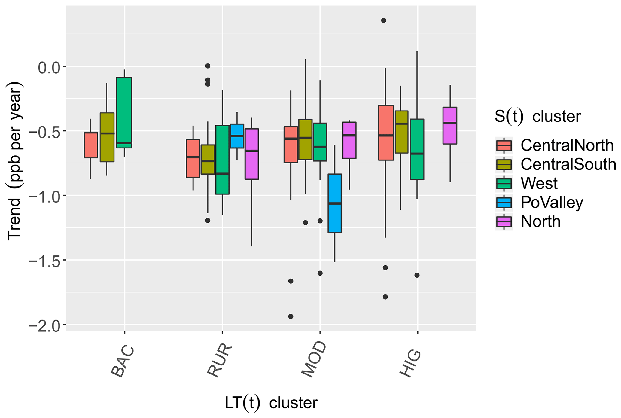
Figure 7 Box plots of meteo-adjusted MTDM trends for the daily mean O₃ LT(t) and S(t) clusters. LT(t) clusters represent a site-type classification, while the S(t) clusters a represent a geographical classification that is influenced by regional climate conditions.

Our results are in line with a modeling sensitivity study, which found negative trends of the 95th percentile of O₃ concentrations at European rural background sites for the period 1995–2014 (Yan et al., 2018). For the shorter time period between 1995 and 2005, downward trends of measured MTDM have been observed in most parts of Europe as well (in the range [−0.12, −0.55] ppb yr⁻¹), with the highest decrease in the Czech Republic, UK, and the Netherlands (on average −1 ppb yr⁻¹) and a very small (nearly flat) decrease in Switzerland (EEA, 2009). In our study, measured MTDM trends (2000–2015) for these regions are in the same range, i.e., the average decrease was estimated between −0.28 and −0.55 ppb yr⁻¹. Smaller trends in Switzerland and central and northeastern Germany have been observed by EEA (2009), which agrees with our result for the CentralSouth cluster sites that showed the smallest average trend of all clusters. The flat trend in Switzerland during 1995–2005 is probably linked to the disproportional decrease in NO_x and VOCs until the beginning of the 2000s, when an inflection point was observed at most polluted sites (Boleti et al., 2018). In Germany, a mixed behavior was observed by the EEA (2009), with the northeastern part showing a stronger decrease and the central and northeastern region showing a smaller decrease. Similar to our differentiation between the clusters, average MTDM trends within the CentralNorth cluster (with northern and northeastern Germany included) were higher, and within the CentralSouth cluster (covering central parts of Germany) these trends were lower.

Figure 8 Annual cycle of daily mean O₃ S(t) for the daily mean S(t) clusters.

4.4 O₃ seasonal cycle trends

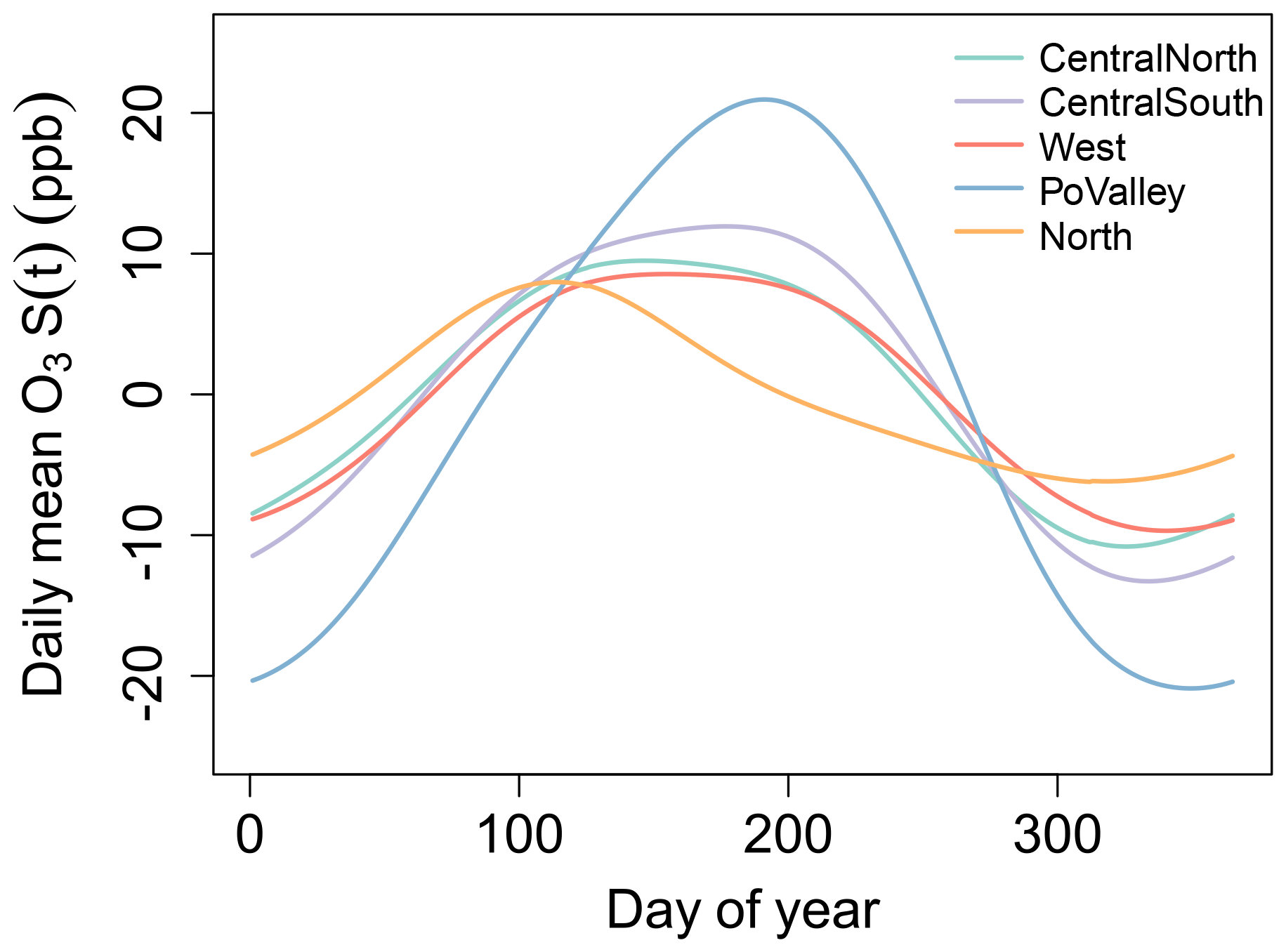
Analysis of S(t) allows for studying the characteristics of the annual cycle of O₃ without influence of short-term meteorological phenomena and long-term variations. Here, the trends of S_max(t), S_min(t) and S_DoM(t) are presented for the five regions identified based on S(t), as calculated from daily mean O₃. In Fig. 8 the average annual O₃ cycles are shown; it is clear that in the PoValley cluster the day of maximum O₃ occurs in summer (June–July), while in the North cluster it occurs around spring (late March–April). This agrees with previous studies that have reported that both the highest average O₃ concentrations and extreme O₃ episodes tend to occur over the central and southern parts of Europe during summer, while over northern Europe they occur during spring (Schnell et al., 2015; Ordóñez et al., 2017). A declining amplitude of S(t) and a simultaneous phase shift towards an earlier time in the year can be observed for the 2000 to 2015 period (Table 2).

Table 2 Linear trends of S_max, S_min and S_DoM for the daily mean O₃ S(t) clusters during 2000–2015: ${}^{**}$ indicates a highly significant trend (p value < 0.01), and – indicates a nonsignificant trend (p value > 0.05).

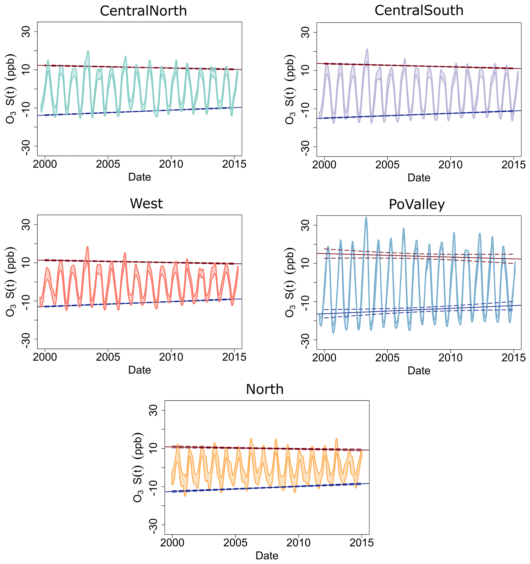
Figure 9 Temporal evolution of S_max and S_min for the daily mean O₃ S(t) clusters together with the average S(t) (bands indicate the average ± the standard deviation). Solid lines show the linear trends of S_max and S_min, and dashed lines show the 90 % confidence interval.

More specifically, an overall decrease in O₃ S_max(t) by around 0.05–0.18 ppb yr⁻¹ and a simultaneous increase in S_min(t) with a rate of around 0.25 ppb yr⁻¹ was observed for all S(t) clusters (Fig. 9). However, in the North cluster the decrease in the S_max(t) was very small and nonsignificant, probably due to the pronounced influence of background O₃ at these sites. The most pronounced shortening of S(t) amplitude can be seen at the PoValley sites, where the downward trend of peak O₃ is largest (Fig. 7). The increase in the S_min(t) may be partially due to the decreased titration of O₃ after reductions of NO_x emissions and is probably due to the increased influx of O₃ towards northern and northwestern Europe and more cyclonic activity in the North Atlantic during winter as well (Pausata et al., 2012). A decrease in the 95th percentile and an increase in the 5th percentile of O₃ for the period 1995–2014 has been also identified in the EMEP network (rural background sites) (Yan et al., 2018). Lower summertime peaks as a result of decreased photochemical production and higher O₃ concentrations during the winter months due to decreased O₃ titration have been found in European air masses between 1987 and 2012 (Derwent et al., 2013) as well.

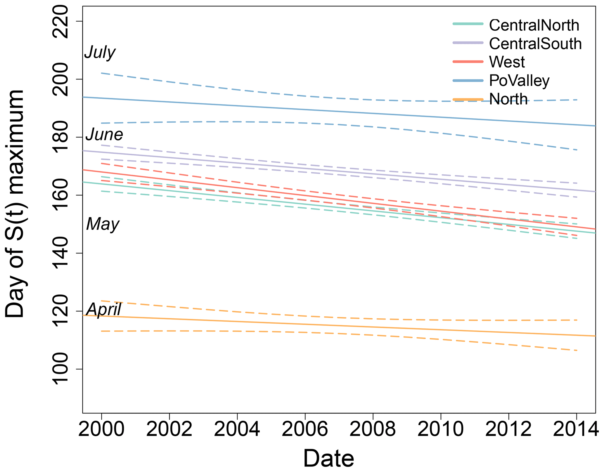
Figure 10 Linear trends of the S_DoMax for the daily mean S(t) clusters (dashed lines show the 90 % confidence interval).

The trend of O₃ S_DoM(t) is negative for all regions, i.e., the occurrence of the day of maximum O₃ has shifted to earlier days within the year with a rate of −0.47 to −1.35 d yr⁻¹ (Table 2, Fig. 10). The observed shift of the day of seasonal maximum might be linked to the increase in emissions in East Asia. The associated strong photochemical reaction rates, convection, and NO_x sensitivity in the tropics and subtropics (Derwent et al., 2008; West et al., 2009; Fry et al., 2012; Gupta and Cicerone, 1998) have probably contributed to increased transport of air pollution to midlatitudes and northern latitudes (Zhang et al., 2016). In addition, changes in meteorological factors may have affected the seasonal variation in O₃. For instance, a similar behavior with an earlier onset of the summer date (the calendar day on which the daily circulation–temperature relationship switches sign) has been observed by Cassou and Cattiaux (2016) using observational data, while Peña-Ortiz et al. (2015) have found that the summer period is extending with a rate of around 2.4 d per decade based on gridded temperature data in Europe. The positive phase of the NAO leads to increased O₃ concentrations in Europe through enhanced transport of O₃ and precursors across the North Atlantic from North America to Europe Creilson et al. (2003). An increase in baseline O₃ related to the prevailing positive NAO index – and the associated westerly flow and intercontinental transport – during the 1990s and the beginning of the 2000s is probably a factor contributing to the increase in the winter S_min O₃ values (Pausata et al., 2012). The enhanced hemispheric transport of air pollutants from North America to Europe is related to increased transport through frontal systems as well (Creilson et al., 2003; Eckhardt et al., 2003). Increased O₃ in winter and spring (but not in summer) might lead to a shifting from a pronounced maximum in late summer to a broader spring–summer peak (Cooper et al., 2014). At the West cluster sites, a slightly stronger shift of the S_DoMax was observed compared to other clusters, while at the North cluster sites the decrease was the smallest. The early spring maximum at the North cluster sites in April (Fig. 8) can be explained by elevated NO_x that is released from PAN and alkyl nitrates that are produced during winter at northern latitudes (Brice et al., 1984; Bloomer et al., 2010).

4.5 O₃ and temperature relationship

The O₃ sensitivity to temperature is a useful metric for validation of precursor reduction scenarios and emission inventories in chemistry–transport models (Oikonomakis et al., 2018). Here, we present the long-term trends of the relationship between the daily maximum O₃ concentrations and daily maximum temperature during the warm season from May to September between 2000 and 2015. Daily maximum O₃ and temperature are chosen in order to represent peak O₃ concentrations formed during the considered days.

Table 3 Linear trends of the O₃–temperature slope (based on daily maximum values) for the daily mean O₃ S(t) clusters for the time period 2000–2015: ${}^{**}$ indicates a highly significant trend (p value < 0.01), and – indicates a nonsignificant trend (p value > 0.05).

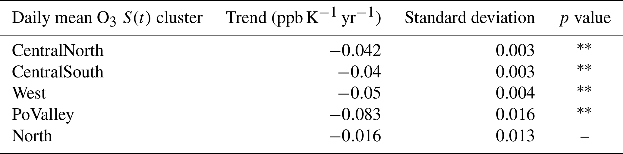
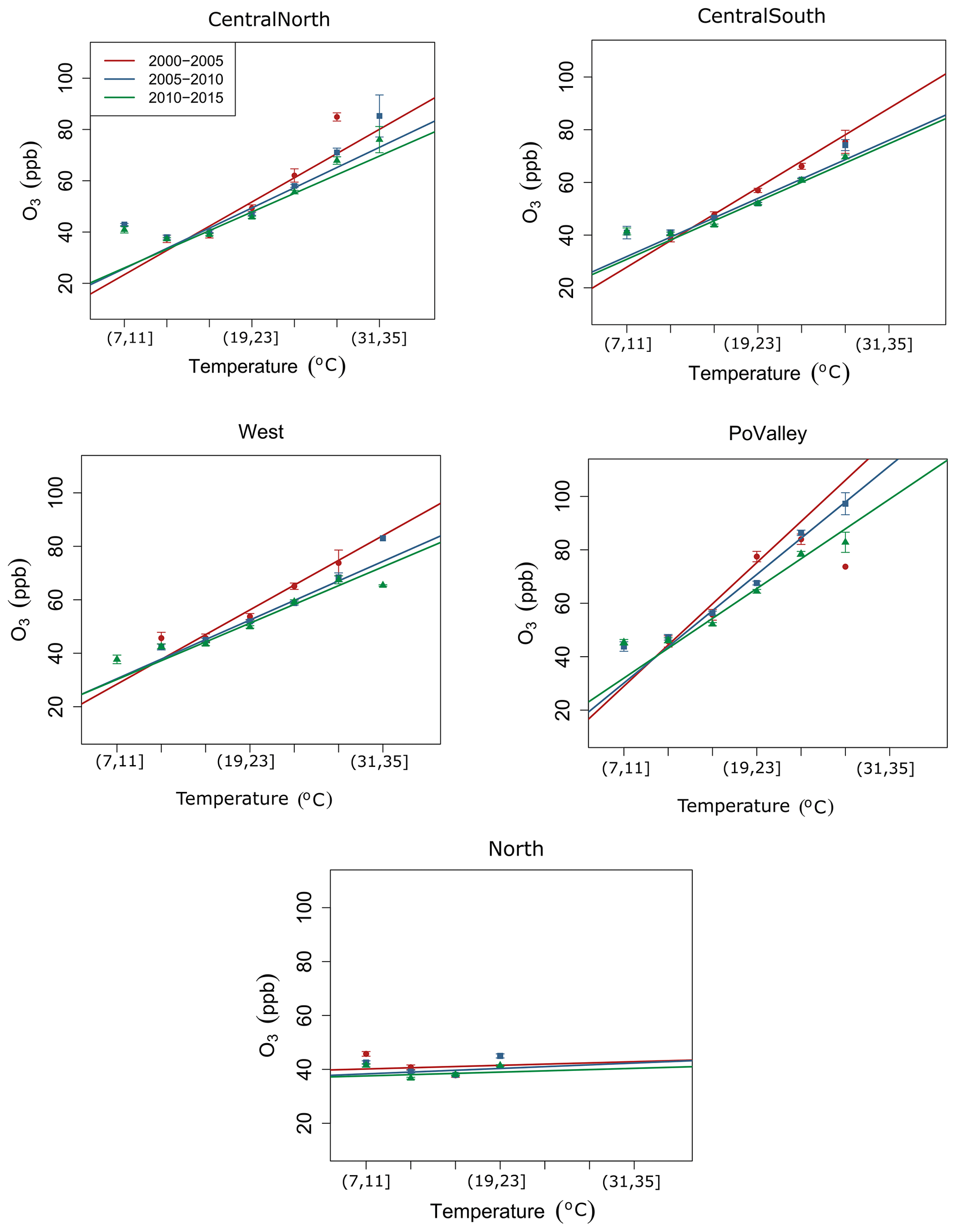
Figure 11 Linear trend of the slope between O₃–temperature daily maximum values for the warm season between May and September. The trends are calculated on the average values for each daily mean S(t) cluster and for the year groups 2000–2005, 2005–2010 and 2010–2015. Points show the mean value for the indicated temperature bin together with the corresponding standard deviation.

Decreasing sensitivity of O₃ with respect to temperature was observed during the considered time period in all regions (Fig. 11). Figure 11 shows the decreasing slopes of linear regression lines of maximum O₃ against temperature for successive year groups. The decrease is consistent for all calculated regional clusters except for the North cluster. For most regions in Europe a significant downward trend of the slope of around 0.04–0.05 ppb K⁻¹ yr⁻¹ was found (Table 3). At PoValley sites the decrease was more pronounced (−0.083 ppb K⁻¹ yr⁻¹) because of large reductions of precursor concentrations in this region, which is characterized by high industrial emissions. Note that the average correlation between O₃ and temperature in that cluster is the highest compared to the other regions. At the North cluster sites the weakest correlation of O₃ to temperature was observed and the trend is nonsignificant. This is expected because at these high latitudes the mean temperature is lower compared to other regions in Europe (Fig. 11); thus, photochemical production of O₃ is weak during the time when O₃ typically reaches its maximum concentration. In addition, in these northern regions the variability of temperature is lower compared to the central and southern parts of Europe, while O₃ concentrations are more influenced by intercontinental transport mechanisms.

Table 4 Linear trends of the O₃–temperature slope (based on daily maximum values) for the daily mean O₃ LT(t) clusters for the time period 2000–2015: ${}^{**}$ indicates a highly significant trend (p value < 0.01), and – indicates a nonsignificant trend (p value > 0.05).

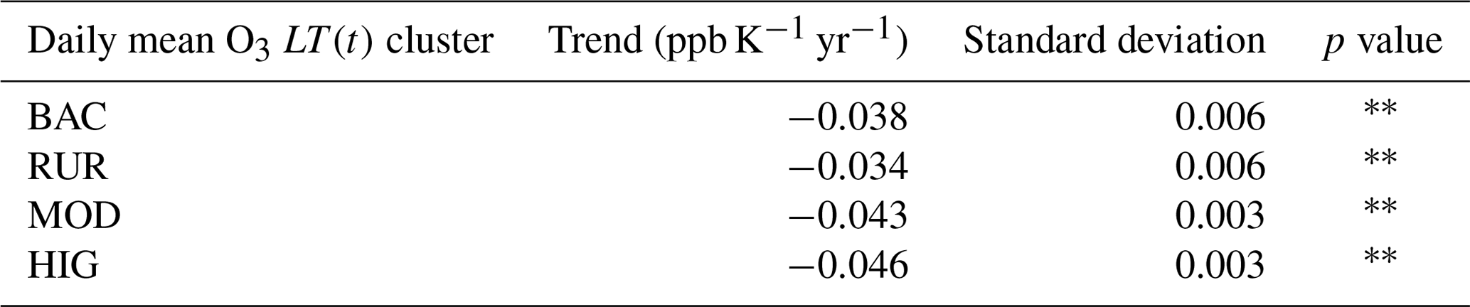
In relation to the LT(t) clusters, it was observed that the higher the pollution burden of the site is, the stronger the trend of O₃ to temperature slope will be (Table 4). As shown here, the HIG and MOD sites have higher trends compared to the clusters BAC and RUR. Our results are in line with a box model study that tested the O₃–temperature relationship under different NO_x level scenarios (Coates et al., 2016). Coates et al. (2016) have shown that at high NO_x conditions O₃ increases more strongly with temperature, while the increase is less pronounced when moving to lower NO_x conditions. Consequently, regional O₃ production has mainly decreased at the most polluted locations, due to considerable reductions of precursor emissions.

5 Conclusions

In this study, a classification of 291 sites across Europe was performed for the time period 2000–2015. The clustering algorithm applied on the long-term changes LT(t) and the seasonal cycle S(t) of daily mean O₃ resulted in a site-type and geographical site classification, respectively. Such a two-dimensional site classification scheme provides an innovative approach for O₃ trends studies in large spatial domains and can be of significant use in model evaluation studies (e.g., Otero et al., 2018). Our approach captures several features of O₃ variations, i.e., pollution level from the LT(t) clustering and influence of the regional climate conditions from the S(t) clustering, and presents a unifying perspective on past studies that report different site-type labels based on cluster analysis using different metrics of O₃ concentrations. The two-dimensional approach offers a tool beyond traditional clustering studies to study the factors that affect O₃ trends. In addition, O₃ time series analysis is complex and benefits from being characterized in different ways, as well as grouped based on several features. The regional differentiation is hampered by sparse or missing measurement sites in some regions, e.g., eastern Europe or the Balkan peninsula. However, in the last few years the number and spatial distribution of sites with longer and more dense measurements has improved.

A trend analysis of deseasonalized mean O₃ concentrations and meteo-adjusted peak O₃ concentrations was implemented for the considered sites. By using LT(t) and S(t) clusters, patterns of O₃ long-term trends across Europe were investigated, based on the multidimensional site classification scheme. Long-term trends of deseasonalized daily mean O₃ are decreasing at rural sites, while at suburban and urban sites they are either stable or slightly increasing. Positive or flat trends indicate that reduction of precursors has been less effective in reducing O₃ concentrations in heavily polluted environments. On the other hand, downward trends in peak O₃ concentrations were observed in all regions as a result of precursor emissions reductions. However, peak O₃ has been decreasing with the smallest rate at higher-altitude sites, especially in the western Europe, possibly due to the influence of background O₃ imported from North America and East Asia.

The analysis of S(t) extrema revealed a decrease in summertime maxima and an increase in wintertime minima, pointing to a decreasing amplitude of the seasonal cycle of O₃. At the same time, the occurrence of the day of maximum has shifted from summer to spring months with a rate of around −0.5 to −1.3 d yr⁻¹. Changes in the S(t) might be attributed to precursor reductions in Europe, changing weather patterns in the North Atlantic and increases in emissions in southern East Asia.

Finally, the sensitivity of O₃ to temperature has weakened since 2000 with a rate of around 0.04 ppb K⁻¹ yr⁻¹, i.e., formation of O₃ became weaker at high temperature conditions, which can be attributed to the decrease in NO_x concentrations. The trend of the sensitivity differs across sites that are influenced by different meteorological conditions.