Determination and climatology of the diurnal cycle of the atmospheric mixing layer height over Beijing 2013–2018: lidar measurements and implications for air pollution

The atmospheric mixing layer height (MLH) determines the space in which pollutants diffuse and is thus conducive to the estimation of the pollutant concentration near the surface. The study evaluates the capability of lidar to describe the evolution of the atmospheric mixing layer and then presents a long-term observed climatology of the MLH diurnal cycle. Detection of the mixing layer heights (MLH_L and MLH${}_{\mathrm{L}}^{\prime }$) using the wavelet method based on lidar observations was conducted from January 2013 to December 2018 in the Beijing urban area. The two dataset results are compared with radiosonde as case studies and statistical forms. MLH_L shows good performance in calculating the convective layer height in the daytime and the residual layer height at night. While MLH${}_{\mathrm{L}}^{\prime }$ has the potential to describe the stable layer height at night, the performance is limited due to the high range gate of lidar. A nearly 6-year climatology for the diurnal cycle of the MLH is calculated for convective and stable conditions using the dataset of MLH_L from lidar. The daily maximum MLH_L characteristics of seasonal change in Beijing indicate that it is low in winter (1.404±0.751 km) and autumn (1.445±0.837 km) and high in spring (1.647±0.754 km) and summer (1.526±0.581 km). A significant phenomenon is found from 2014 to 2018: the magnitude of the diurnal cycle of MLH_L increases year by year, with peak values of 1.291±0.646 km, 1.435±0.755 km, 1.577±0.739 km, 1.597±0.701 km and 1.629±0.751 km, respectively. It may partly benefit from the improvement of air quality. As to converting the column optical depth to surface pollution, the calculated PM_2.5 using MLH_L data from lidar shows better accuracy than that from radiosonde compared with observational PM_2.5. Additionally, the accuracy of calculated PM_2.5 using MLH_L shows a diurnal cycle in the daytime, with the peak at 14:00 LST. The study provides a significant dataset of MLH_L based on measurements and could be an effective reference for atmospheric models of surface air pollution calculation and analysis.

1 Introduction

The height of the mixing layer (MLH) is a crucial parameter for near-surface air quality forecasts, pollutant dispersion and the quantification of pollutant emissions (Haeffelin et al., 2012; Seibert et al., 2000; Baars et al., 2008; Liu and Liang, 2010; de Bruine et al., 2017). The pollutants discharged in the boundary layer diffuse vertically under the drive of turbulence (Gan et al., 2011; Monks et al., 2009; Guo et al., 2016) and finally become completely mixed over this layer if sufficient time is given (Emeis et al., 2008). The MLH determines the space in which pollutants diffuse and is thus conducive to the estimation of the pollutant concentration near the surface, which might be detrimental to the health of humans and ecosystems (Emeis et al., 2007; Collaud Coen et al., 2014; Singh et al., 2016; Mues et al., 2017).

Within the planetary boundary layer (PBL) the height of the mixing layer (ML) is defined as the height up to which vertical dispersion by turbulent mixing of air pollutants takes place due to the thermal structure of the PBL (Seibert et al., 2000; Schafer et al., 2006; Emeis et al., 2007). The MLH depends largely on the synoptic weather situation (Emeis et al., 2008). The MLH can be estimated by the detection of variance in the mechanical turbulence, the temperature enabling convection or the substance content in the low troposphere. Singh et al. (2016) investigated the evolution of the local boundary layer in the central Himalayan region using a radar wind profiler detecting wind components based on the signal-to-noise ratio profile. Collaud Coen et al. (2014) compared MLH measurements of a microwave radiometer from an atmospheric temperature profile with other measurements in the Swiss Plateau. Mues et al. (2017) used a ceilometer to retrieve the MLH based on the aerosol backscatter signal in the Kathmandu Valley. These measurements are based on different atmospheric parameters, different measuring instruments and various analysis algorithms, leading to MLH results obtained by different methods being inconsistent (Collaud Coen et al., 2014).

In order to move from the general definition to practical measurements, it is necessary to separately consider the structure of the convective boundary layer (CBL) and the stable boundary layer (SBL). In the case of fair weather days, the PBL height has a well-defined structure and diurnal cycle (Collaud Coen et al., 2014; see Fig. S1 in the Supplement). The PBL development under strong convection driven mainly by solar heating is called the CBL (Collaud Coen et al., 2014). The nocturnal SBL shows a more complex internal structure, including a stable layer caused by radiative cooling from the ground, and gradually merges into a neutral layer called the residual layer (RL) (Stull, 1988; Mahrt et al., 1998; Salmond and McKendry, 2005; Collaud Coen et al., 2014). The RL height is the top of the neutral layer and the beginning of the stable free troposphere. The pollutants discharged from the surface at night are restricted to the SBL, while the pollutant emissions from past days tend to stay in the RL. In addition to the dominance of the CBL in the afternoon, the SBL and neutral boundary layer may be formed under certain weather conditions (Stull, 1988; Poulos et al., 2002; Medeiros et al., 2005; Zhang et al., 2018)

Since most atmospheric column aerosol particles are usually present in atmosphere below the MLH, the MLH can be used to convert the aerosol optical thickness of the column observed by sun photometers and satellites to the concentration of near-surface pollutants (Sifakis et al., 1998; Dandou et al., 2002; Emeis et al., 2007). Particulate can be used as an important indicator of atmospheric layering because its vertical distribution is strongly affected by the thermal structure of the atmosphere (Neff and Coulter, 1986). Provided the vertical aerosol distribution adapts rapidly to the variational thermal dynamics of the boundary layer, the MLH can be retrieved from the analysis of this aerosol distribution (Emeis et al., 2008).

By the measurement of the profile of aerosol, lidar offers a direct and continuous way to monitor the diurnal cycle of the different layers constituting the PBL (Seibert et al., 2000; De Haij et al., 2006; Emeis et al., 2008; Liu and Liang, 2010; Tang et al., 2016; Su et al., 2017, 2019). With recent upgrades of hardware, a ceilometer, also known as an automated low-power lidar or an automated lidar–ceilometer (ALC), has been demonstrated to capably determine the MLH (Wiegner et al., 2006; Martucci et al., 2007, 2010; Geiß et al., 2017; Kotthaus and Grimmond, 2018; Mues et al., 2017). Recent studies have compared remote sensing measurements (lidar, radar wind profiler, microwave radiometer) with radiosonde (RS) (Wiegner et al., 2006; Milroy et al., 2012; Sawyer and Li, 2013; Cimini et al., 2013; Tang et al., 2016; Singh et al., 2016; Mues et al., 2017; Su et al., 2019), with which convection weather cases have good correlation with differences of 100–300 m, while non-convective weather conditions lead to much larger differences in the MLH estimations if the approaches are intended to measured different structures of the ML such as the CBL, SBL or RL (Collaud Coen et al., 2014). Meteorological radiosondes usually acquire the MLH in the morning (08:00 LT) and at night (20:00 LT), when the diurnal cycle of the ML combined with the stable and convective PBL cannot be well characterized.

In existing studies, numerical simulations, ground-based remote sensing or meteorological radiosondes are used to obtain the characterization of the MLH during short time periods in Beijing, mainly focusing on heavy pollution events (Yang et al., 2005; Quan et al., 2013; Hu et al., 2014; Zhang et al., 2015), which underscores the scarceness of continuous high-resolution measurements for a long time period. Depending on the measured atmospheric parameters and observational uncertainties, different measurement approaches may reveal different aspects of PBL structure (Seibert et al., 2000; Seidel et al., 2010; Beyrich and Leps, 2012). Thus, it is of great significance to apply consistent algorithms to consistent types of atmospheric structure parameters when comparing the MLH from different times.

The main aim of this study, therefore, is to present a long-term observed climatology of the MLH diurnal cycle based on lidar observations. For that, the capability of lidar to describe the diurnal evolution of the mixing layer height is evaluated first. The data and methods used are described in Sect. 2. Section 3 contains the results and discussion, which consist of the comparison of lidar-derived MLH with radiosonde measurements, the climatology of the MLH in Beijing, and implications for surface pollution retrieval. Then, it is concluded in Sect. 4.

2 Data and methods

2.1 Site and lidar measurements

Beijing is the capital of China with about 20 000 000 citizens. Beijing is located on flat terrain in the North China Plain (altitude of 20–60 m), with the Taihang Mountains in the west and the Yan Mountains in the north (altitude of 1000–1500 m). Similar to many other metropolitan areas, Beijing suffers from episodes of poor air quality, in particular fine particulate matter (PM_2.5). In the study, the observatory (116.379^∘ E, 40.005^∘ N) in the metropolitan area of Beijing is located on the building roof (59 m a.s.l.) of the Institute of Remote Sensing and Digital Earth, Chinese Academy of Sciences. A micro-pulse lidar (CE370, CIMEL, France) was used to detect the atmospheric aerosol structure at this site. The laser used is a frequency-doubled Nd:YAG with pulse repetition frequency 4.7 kHz and energy 8–20 µJ. The CE370 operates at a wavelength of 532 nm with the vertical resolution of 15 m and can detect a long-range profile up to 30 km every second. For the enhancement of the signal-to-noise ratio, 60 profiles are averaged to restore as one, with the time resolution of 1 min. The signal received from the lidar is processed by the subtraction of atmospheric background using the averaged value of the signal received from the height between 22 and 30 km. There are remnants of the previous signal in the system in the absence of optical signal reception, and these signals are called after-pulses. They are monitored every week and removed from the receive signal. Due to the design of the lidar, the received view close to the ground does not completely coincide with the transmitted view. There is a detection blind area in the lidar, and a geometric overlap factor is used to correct the mismatch of the field of view. Then, the correction of the range (range-corrected signal, RCS) is used to retrieve the MLH. The profile of the RCS is expressed as f (z), with z the measurement height. Logarithm calculation of the RCS (expressed in In(${\mathit{\beta }}_{\mathrm{532}}^{\prime }\left)\right)$ is presented in the lidar image (Campbell et al., 2003; Yan et al., 2014; Su et al., 2019). MLH estimation from lidar systems is based on the measurement of the sudden drop in aerosol backscatter at the top of the mixing layer (Seibert et al., 2000). The period of lidar measurements is from 2013 to 2018, nearly 6 years. Except for the lidar data for 2013 mainly in winter and spring (months 1–4 and 11–12), the measurements for 2014–2018 are all annual continued observations.

2.2 MLH derived from lidar

Wavelet transforms are commonly used in many studies for MLH determination from lidar observations (Cohn and Angevine, 2000; Davis et al., 2000; Brooks, 2003; De Haij et al., 2006; Baars et al., 2008; Su et al., 2019). When the maximum value of the attenuated backscattering profile convolved with the Haar function is reached, the corresponding height is the MLH. The equation of the wavelet is defined as follows:

$$\begin{array}{}\text{(1)}& h\left({\displaystyle \frac{z-b}{a}}\right)=\left\{\begin{array}{l}\mathrm{1},b-\frac{a}{\mathrm{2}}\le z\le b;\\ -\mathrm{1},b<z\le b+\frac{a}{\mathrm{2}}\\ \mathrm{0},\mathrm{else}\end{array}\right.,\end{array}$$

where b is the transformation of the equation, the equation is cantered and a is the expansion of the equation. The equation of the wavelet covariance transformation W_f(a,b), namely the convolution of f(z) with the wavelet function, is defined as follows:

$$\begin{array}{}\text{(2)}& W_f(a,b)={\displaystyle \frac{\mathrm{1}}{a}}\underset{z_b}{\overset{z_t}{\int }}f\left(z\right)h\left({\displaystyle \frac{z-b}{a}}\right)\mathrm{d}z,\end{array}$$

where f(z) represents the RCS at different heights, z_b denotes the lower limit of the height of the profile and z_t represents the upper limit of the height. A valid MLH_L is detected, corresponding to the value b when W_f(a,b) reaches the biggest local maximum with a coherent scale of a (Brooks, 2003; De Haij et al., 2006; Emeis et al., 2008). In this study, the expansion of a is selected as 420, 435 and 450 m, and the final W_f(a,b) is calculated from the averaged corresponding values. Another layer, called MLH${}_{\mathrm{L}}^{\prime }$, is detected simultaneously by the first local maximum W_f(a,b) from z_b, which is assumed to be smaller than or equal to MLH_L (De Haij et al., 2006; Mues et al., 2017). Actually, every local maximum corresponds to an aerosol layer and several internal layers appear, making the allocation of a local maximum to an atmospheric feature very difficult (Morille et al., 2007; Geiß et al., 2017; Poltera et al., 2017; Kotthaus and Grimmond, 2018). Since the absolute maximum in the vertical gradient of the lidar profiles is characterized by a rapid decrease in pollutant concentrations, the MLH_L can be associated with the CBL height during daytime (Haeffelin et al., 2012; Poltera et al., 2017) and the RL height during nighttime (Collaud Coen et al., 2014). However, the interpretation of the first local maximum (MLH${}_{\mathrm{L}}^{\prime }$) is critical.

To form a diurnal cycle of the MLH from these several layers, a geodesic approach was applied to pathfinderTURB (Poltera et al., 2017), while COBOLT (Geiß et al., 2017) uses a time–height tracking approach with moving windows. Nevertheless, these methods are all based on the selection of the lowest detected aerosol layer. The height of the lowest detected aerosol layer was regarded as the daytime MLH and the nocturnal stable boundary layer, as reported by Mues et al. (2017) and Kotthaus and Grimmond (2018), respectively. Su et al. (2019) developed a depend time and depend stability (DTDS) algorithm, started with the lowest point and tracked depending on the time and stability, but the nocturnal MLH with SBL height is not evaluated. The detection of nocturnal boundary layer heights, in contrast to the residual layer, is a major challenge (Haeffelin et al., 2012; Lotteraner and Piringer, 2016; de Bruine et al., 2017). Thus, one of the objectives of this study is to investigate the usefulness of MLH${}_{\mathrm{L}}^{\prime }$ from CE-370 to capture the SBL height over Beijing.

MLH retrievals are eliminated if a cloud flag is marked when the cloud base is found within 6 km of the surface, and a threshold is selected to distinguish between clouds and aerosol layers. To improve the retrieval, a Gaussian filter is applied to retrievals to smooth the temporal variability, and unrealistic outliers are deleted. Due to the limitation of the algorithm and insufficient lidar overlap, the minimum range of the MLH calculation from CE-370 is on the order of 250 m, which is higher than the order of 50 m with a ceilometer. This is due to the optical design of the ceilometer using the same lens for the emitter and the receiver optical paths, which suffers from a low signal-to-noise ratio and provides a lower overlap with the limited power transmitted from the optical design. Detecting significant vertical gradients of attenuated backscatter can be challenging on a clear day when aerosol content is low (Eresmaa et al., 2012; Haeffelin et al., 2012). Compared to CE-370, a ceilometer usually needs a large-scale temporal and vertical average at the cost of a reduction of retrieval in relatively clean atmospheric conditions (de Bruine et al., 2017; Kotthaus and Grimmond, 2018).

2.3 MLH from radiosonde

Radiosonde (RS) measurements are one of most widely used methods, especially in China, to derive the SBL height and CBL height due to the ability to characterize the thermodynamic and dynamic states of the boundary layer (Piringer et al., 2007; Seidel et al., 2010; Guo et al., 2019). Meteorological radiosondes perform measurements at the international standard weather station (39.484^∘ N, 116.282^∘ E), which was located nearly 11 km from the lidar station. It includes two categories: conventional observations around the year, which are performed at 00:00 UTC (08:00 LST) in the morning and at 12:00 UTC (20:00 LST) in the evening each day, and intensified observations only in summer, which are taken at 06:00 UTC (14:00 LT) in the afternoon. The observed meteorological parameters include atmospheric pressure (P), temperature (T), relative humidity (RH), wind speed (WS) and wind direction (WD).

The bulk Richardson number (Ri_b) is a dimensionless parameter combining the thermal energy and the vertical wind shear; it is widely used in MLH climatology (Seidel et al., 2012; Collaud Coen et al., 2014). Ri_b is defined as the ratio of turbulence associated with buoyancy to that induced by mechanical shear, which is expressed as

$$\begin{array}{}\text{(3)}& R{i}_{\mathrm{b}}={\displaystyle \frac{gz(\mathit{\theta }\left(z\right)-\mathit{\theta }(z_{\mathrm{s}}\left)\right)}{{\mathit{\theta }}_{z_{\mathrm{s}}}(U^{\mathrm{2}}\left(z\right)+V^{\mathrm{2}}\left(z\right))}},\end{array}$$

where z is the height (z>z_s, the subscript “s” denotes the surface), θ characterizes the virtual potential temperature, U and V indicate the two horizontal wind velocity components, and g represents the Earth's gravitational constant. The MLH_RS corresponds to the first elevation z, with Ri_b greater than a critical threshold taken as 0.25 (Stull, 1988; Seidel et al., 2012; Guo et al., 2016, 2019). In most cases, the exact threshold value has only a small impact on the PBL height due to the large slope of Ri_b in this interval (Collaud Coen et al., 2014).

2.4 Air pollution model

Data on the MLH are usually combined within an atmospheric model to obtain the surface air pollutant concentration. For example, PM_2.5 remote sensing (PMRS) models, such as that derived by Zhang and Li (2015), have the ability to calculate the mass concentration of PM_2.5 above the ground. The PMRS method is designed to employ currently available remote sensing parameters, including aerosol optical depth (AOD), fine-mode fraction (FMF), planetary boundary layer height (PBL height) and atmospheric relative humidity (RH), to derive PM_2.5 from instantaneous remote sensing measurements under different pollution levels (Zhang and Li, 2015; Li et al., 2016; Yan et al., 2017). PM_2.5 is calculated following the PMRS model as

$$\begin{array}{}\text{(4)}& {\mathrm{PM}}_{\mathrm{2.5}}={\displaystyle \frac{\mathrm{AOD}}{\mathrm{PBLH}}}\cdot {\displaystyle \frac{\mathrm{FMF}\cdot {\mathrm{VE}}_{\mathrm{f}}\left(\mathrm{FMF}\right)\cdot {\mathit{\rho }}_{\mathrm{2.5},\mathrm{dry}}}{f_{\mathrm{0}}\left(\mathrm{RH}\right)}},\end{array}$$

where AOD indicates aerosol optical depth and FMF represents the fine-mode fraction; VE_f is the ratio of the volume and extinction of fine-mode aerosol, which can be calculated from FMF as VE_f(FMF)=0.2887FMF²-0.4663FMF+0.356. The parameter ρ_2.5,dry indicates the density of dry PM_2.5, while f₀(RH) represents the particle hydroscopic growth function, which is f₀(RH)= (1-RH/100)⁻¹. The PBL height can be derived from remote sensing and radiosonde measurements.

Figure 1 (a) Daily backscatter profiles from lidar for 2–4 March 2017. The lines connected by black dots in the figure represent the retrieved MLH_L, while white dots line indicate the MLH${}_{\mathrm{L}}^{\prime }$, and the top of the purple triangle indicates the MLH_RS identified from radiosonde. The horizontal axis represents the local standard time (LST), and the vertical axis represents the height. The color bar denotes the logarithm of the attenuated backscattering coefficient (In(${\mathit{\beta }}_{\mathrm{532}}^{{}^{\prime }}\left)\right)$. (b, c, d) The vertical profile of RCS (orange curve) from lidar and the wavelet coefficient (red curve) of RCS, as well as the vertical profile of temperature (T) (blue curve) and relative humidity (RH) (cyan curve) for (b) 20:00 LST on 3 March 2017, (c) 08:00 LST on 4 March 2017 and (d) 20:00 LST on 4 March 2017, as indicated by the white-outlined triangle in panel (a).

All the parameters are observed by the instruments employed in the same observatory as the lidar. The optical parameters of the column aerosols (AOD and FMF) are obtained by a sky–sun photometer (CE318-DP, CIMEL, France), which is affiliated with the Aerosol RObotic NETwork (AERONET) (Holben et al., 1998; Dubovik et al., 2000). Measurements are automatically scheduled with direct sun irradiance measurements of about 15 min each and angular sky radiance scanning of about 1 h each (Li et al., 2015; Che et al., 2014; Wang et al., 2019). Atmospheric meteorological data (relative humidity, wind speed, wind direction, etc.) are obtained by an automatic meteorological monitoring station (BLJW-4). The PM_2.5 mass concentration is obtained by a PM_2.5 monitor (BAM-1020; MetOne, USA), which shows good agreement with the measurements of the national monitoring network near the observatory. All the data are quality-controlled and calculated as 1 h averages, and the measurement period is from 2014 to 2018. The MLH obtained from both lidar and radiosonde within the period is used in the model to calculate the surface PM_2.5. For convenient comparison with air quality and meteorological parameters, all MLH results are 1 h averaged.

3 Results and discussion

3.1 MLH operational measurement

A selection of typical atmospheric conditions included in the dataset of lidar measurements is plotted in Figs. 1–4. The heights of the mixing layer, MLH_L and MLH${}_{\mathrm{L}}^{\prime }$, are obtained from different criteria using the wavelet covariance transform method. As shown in Fig. 1, the development of a convective mixing layer could clearly be observed, with a sharp decrease in aerosol backscatter between the mixing layer and the free atmosphere. MLH_RS is also presented, accompanied by the evolution of MLH_L and MLH${}_{\mathrm{L}}^{\prime }$.

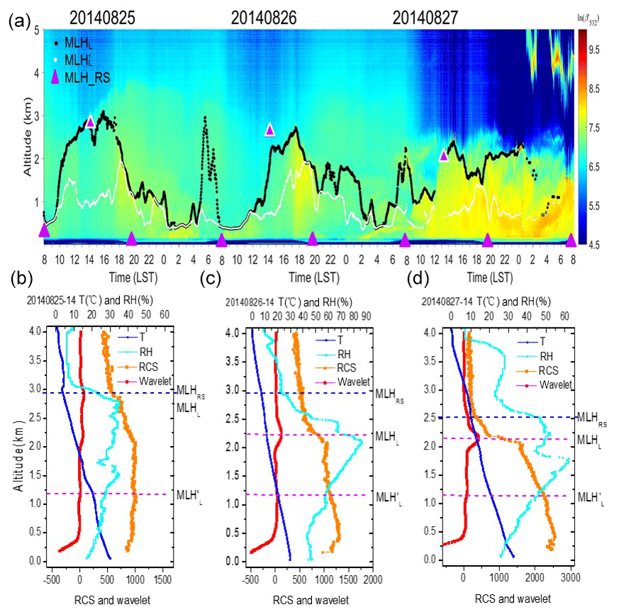
Figure 2 Similar to Fig. 1, but for (a) 25–27 August 2014, and with vertical profiles for (b) 14:00 LST on 25 August 2014, (c) 14:00 LST on 27 August 2014 and (d) 20:00 LST on 27 August 2014.

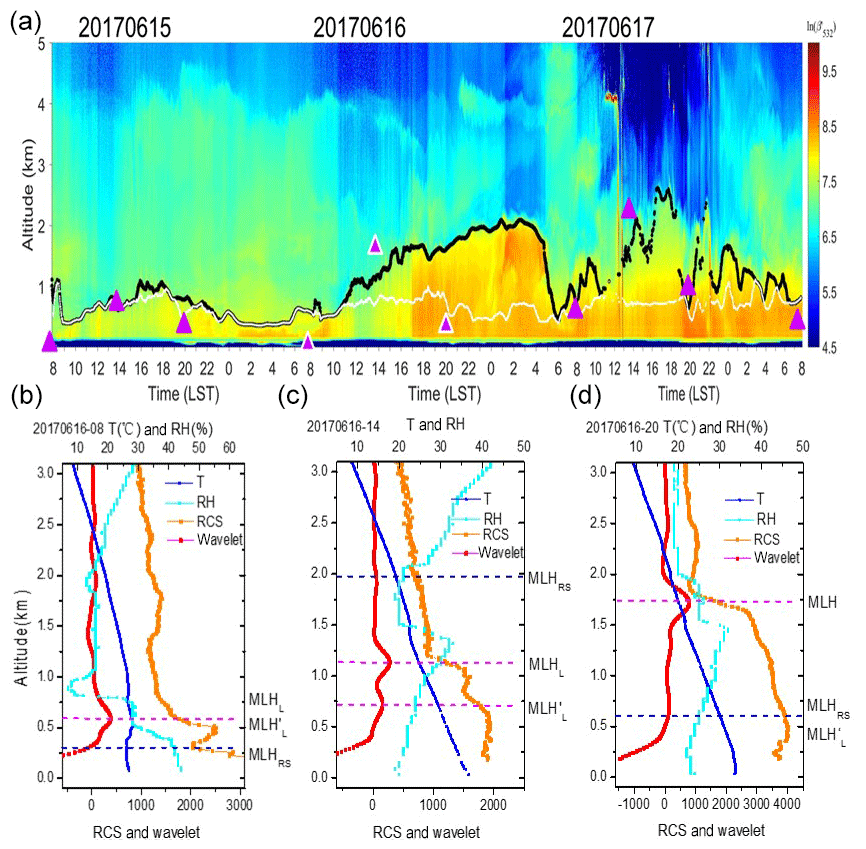
Figure 3 Similar to Fig. 1, but for (a) 15–17 June 2017, and with vertical profiles for (b) 08:00 LST on 16 June 2017, (c) 14:00 LST on 16 June 2017 and (d) 20:00 LST on 16 June 2017.

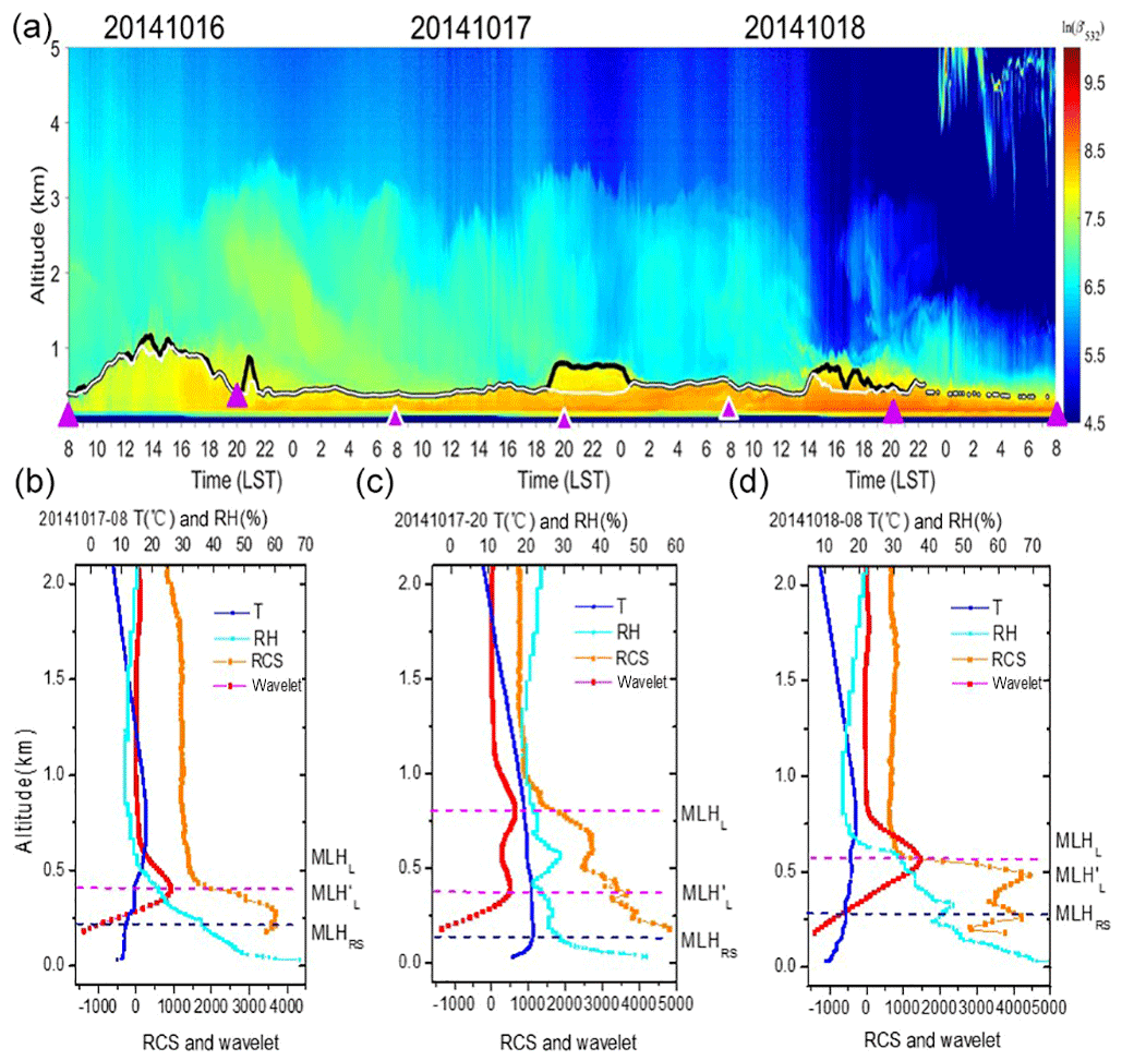
Figure 4 Similar to Fig. 1, but for (a) 16–18 October 2014, and with vertical profiles for (b) 08:00 LST on 17 October 2014, (c) 20:00 LST on 17 October 2014 and (d) 08:00 LST on 18 October 2014.

As shown in Fig. 1a , MLH_L and MLH${}_{\mathrm{L}}^{\prime }$ increase at sunrise. On 2 March 2017, MLH_L and MLH${}_{\mathrm{L}}^{\prime }$ show an obvious diurnal cycle, with a maximum up to 1.0 km. During the evening of 3 March 2017 and the early morning of 4 March 2017, the aerosol layers present two visually obvious layers; MLH${}_{\mathrm{L}}^{\prime }$ characterizes the first layer height and MLH_L represents the upper-layer top. On the next day, due to the existence of cloud, the MLH results are discrete. In the evening and early morning, MLH${}_{\mathrm{L}}^{\prime }$ deviated from MLH_L and approached MLH_RS. As shown as the vertical profile from the lidar (RCS, wavelet) and radiosonde (RH, T) at 20:00 (LST) on 3 March 2017 (Fig. 1b), both MLH${}_{\mathrm{L}}^{\prime }$ and MLH_RS demonstrate 0.53 km, while MLH_L shows 1.22 km. Figure 1c indicates that MLH${}_{\mathrm{L}}^{\prime }$ (0.86 km) approaches MLH_RS (0.61 km), although it is a little higher (0.25 km) and much lower than MLH_L (1.62 km). In these cases, the result of MLH${}_{\mathrm{L}}^{\prime }$, indicated by the first local maximal aerosol gradient, agrees well with MLH_RS. However, this is not always true, as shown in Fig. 1d. MLH${}_{\mathrm{L}}^{\prime }$ (0.752 km) is much higher than MLH_RS (0.243 km) but equal to MLH_L. It is related to the fact that the stable layer height obtained from radiosonde in this case is out of the range of lidar detection (0.255 km), so MLH${}_{\mathrm{L}}^{\prime }$ from lidar is disabled to determine the stable layer height.

In the summertime (JJA) when the radiosonde is additionally launched at 14:00 LST to detect the convective boundary layer, it can provide the comparison between lidar and RS measurements in the afternoon. As shown in Fig. 2a, MLH_L undergoes a rapid increase in the morning and reaches the peak in the afternoon, while MLH${}_{\mathrm{L}}^{\prime }$ grows with a smaller magnitude. On 25 and 26 August 2014, the aerosol load is relatively low, and MLH_L reaches the peak at around 3.0 km in the afternoon, while a lower MLH_L peak on 27 August 2014 is observed with a high aerosol content. In the afternoon on these three days, MLH_L is consistent with MLH_RS, while MLH${}_{\mathrm{L}}^{\prime }$ is frequently under MLH_RS. The measurement of RS in the evening and early morning presents very low values at 0.2–0.3 km. The detailed information represented in Fig. 2b shows that MLH_L is equal to MLH_RS, which reaches up to 2.95 km, while MLH${}_{\mathrm{L}}^{\prime }$ is only at 1.24 km. Under clear convective conditions on 25 and 26 August 2014, when there are weak vertical gradients in the aerosol load indicated by a weak RCS, lidar can still obtain good MLH results compared to radiosonde, as shown in Fig. 2c and d with MLH_L (2.25 and 2.18 km) approaching MLH_RS (2.96 and 2.50 km). The slightly lower value of MLH_RS is associated with the fact that aerosol within the mixing layer needs some time to adjust to the thermal structure, and there is a delay in reaching the thermodynamic PBL height (Stull, 1988; Collaud Coen et al., 2014).

As shown in Fig. 3a, the peaks of the three days gradually increase, with values of 1.0, 2.0 and 2.5 km. Due to the high temporal variability of the distribution of aerosol, MLH_L presents discontinuity on 17 June 2017. MLH_L presents good evolution of the mixing layer height on 15 and 17 June 2017 compared to MLH_RS. MLH${}_{\mathrm{L}}^{\prime }$ corresponds to MLH_RS for most of the time in the morning and evening from 15 to 17 June 2017. But when the stable layer height from radiosonde is around or below 0.25 km, for example at 08:00 LST on 16 June 2017 with the RS measurement of 0.27 km (Fig. 3b), MLH${}_{\mathrm{L}}^{\prime }$ misses the height of the SBL but points to the height of the residual layer (0.61 km). When the stable layer height is higher than 0.25 km, MLH${}_{\mathrm{L}}^{\prime }$ (0.62 km) tends to approach to MLH_RS (0.62 km) (Fig. 3d). However, in the afternoon MLH_L was closer to MLH_RS compared to MLH${}_{\mathrm{L}}^{\prime }$ (Fig. 3c). As shown in Fig. 4a , MLH_L (MLH${}_{\mathrm{L}}^{\prime }$) presents the diurnal cycle with the maximum of 1.2 km, while the next two days stay stable the whole day, and the height of the SBL is missed by MLH${}_{\mathrm{L}}^{\prime }$ (Fig. 4b–d).

3.2 Intercomparison of different MLH approaches

A comparison of MLH estimated by lidar and radiosonde at 08:00 and 20:00 LST, is shown in Fig. 5. The same observation period of nearly 6 years (2013–2018) is considered, during which the data are continuous except for 2013. As shown in the histograms in Fig. 5, the total column is the annual relative frequency, and the different colors indicate the contribution of each season to the total. There is a wide discrepancy between MLH_L and MLH_RS at 08:00 and 20:00 LST. The frequency of MLH from a radiosonde lower than 0.25 km is nearly 35 %, whereas there are no data for MLH_L from lidar due to the limited detection range. This lower value mainly occurs in winter and autumn, when MLH tends to be lower (Tang et al., 2016). Specifically, the rate of MLH_L from lidar lower than 0.5 km is nearly 18 % and 12 % at 08:00 and 20:00 LST, respectively, while the corresponding frequency for radiosonde is beyond 75 % and 66 %. The frequency of the larger MLH_L value at 20:00 LST is bigger than that of 08:00 LST from both lidar and radiosonde. It is reasonable that the residual layer has not yet collapsed entirely at 20:00 LST, while the CBL has not developed well in the early morning. As for the MLH${}_{\mathrm{L}}^{\prime }$, its distribution trend is more similar to MLH_RS than MLH_L (see Fig. S2), and the correlation between MLH${}_{\mathrm{L}}^{\prime }$ and MLH_RS is a little higher than that between MLH_L and MLH_RS, in spite of the fact that it is still not good (see Figs. S3 and S4). This indicates that MLH${}_{\mathrm{L}}^{\prime }$ has the potential to determine the SBL height as radiosonde does.

As for the seasonal variation of both lidar and RS measurements at 08:00 LST, the frequency of the larger MLH_L value in summer is minimal, indicating that the summer MLH is lower than in other seasons. As for radiosonde, MLH_L lower than 0.25 km is mostly distributed in winter, with a rate of around 15 % for both 08:00 and 20:00 LST, and the frequency decreases rapidly when MLH_L becomes higher than 0.25 km.

The poor agreement between MLH from lidar and MLH_RS is also reported in the study of Su et al. (2019), in which it is shown that the correlation of the PBL height measurement between the lidar and radiosonde is 0.14 at 06:30 LST. The significant scatter in the morning and evening is associated with the complicated structure of the boundary layer, as indicated by the existence of a stable boundary layer and residual layer (Su et al., 2019; Tang et al., 2016). In this study, regardless of MLH_L and MLH${}_{\mathrm{L}}^{\prime }$, more than 35 % of the measurements of the SBL height are not within the scope of the lidar detection. Additionally, in the evening and early morning in some cases, a sufficiently clear variety cannot be found in the backscatter profile at the top of the SBL within the previously well-mixed layer (Russell et al., 1974; Seibert et al., 2000).

The comparison of MLH_L and MLH_RS at 14:00 LST in summer is presented in Fig. 6, with both mainly indicating the CBL height. MLH_L shows very good agreement with MLH_RS, with a correlation coefficient of 0.692 and a root mean square error (RMSE) of 0.573 km. It is noted that the slope of the linear fitting line is smaller than the 1:1 line, indicating that MLH_RS tends to be larger than MLH_L in the afternoon, which is consistent with the case study. Although the comparison is only for summer, it can be generally concluded that MLH_L from lidar in the afternoon characterizes the CBL height with good accuracy. As shown in Fig. S4, the correlation of MLH${}_{\mathrm{L}}^{\prime }$ and MLH_RS at 14:00 LST is 0.330, and the value of MLH${}_{\mathrm{L}}^{\prime }$ is generally lower than MLH_RS, indicating that it is overall unsuitable for MLH${}_{\mathrm{L}}^{\prime }$ to describe the CBL height in the afternoon.

In fact, complete agreement is not expected between MLH_L (MLH${}_{\mathrm{L}}^{\prime }$) derived from lidar and MLH_RS from radiosonde for several reasons. First, the two systems measure different atmospheric parameters (aerosol for lidar and temperature, humidity, wind for radiosonde) with varying height resolution and accuracy, and these parameters are influenced in different ways by the processes occurring within the PBL (Seibert et al., 2000). Additionally, it is difficult to identify a clear upper boundary of the mixing layer because the measured parameter is actually not a fixed point but rather a transition layer between two atmospheric states (Stull, 1988; Garratt, 1992; Collaud Coen et al., 2014).

A dataset containing nearly 6 years of measurements in Beijing is used for assessment of the overall performance of the wavelet MLH algorithm (MLH_L and MLH${}_{\mathrm{L}}^{\prime }$) with respect to the diurnal availability, as shown in Fig. 7. It can be seen that the expected shape representing the growth of a convective mixing layer is observed. Owing to solar heating of the surface, when the convective layer begins to rise due to upward convection in the early morning and the nocturnal residual layer tends to collapse, MLH_L from lidar presents the minimal value. After that, MLH_L grows continuously and reaches its maximum height around 15:00 LST, with the value of 1.449, similar to results found for Vienna (Lotteraner and Piringer, 2016) and Berlin (Geiß et al., 2017). The shaded areas indicate the temporal variability as calculated from the standard deviation of MLH_L (MLH${}_{\mathrm{L}}^{\prime }$). It is on the order of 600 m for MLH_L (300 m for MLH${}_{\mathrm{L}}^{\prime }$) during 09:00–15:00 LST, while the other period is on the order of 700 km (400 m for MLH${}_{\mathrm{L}}^{\prime }$). The larger standard deviation is attributed to the variability of the residual layer.

Figure 5 Comparison of the frequency distribution of all MLH_L (2013–2018) retrieved from lidar and MLH_RS from radiosonde with supplementary information on seasonal variation. The MLHs from (a) lidar and (b) radiosonde at 08:00 (LST) as well as (c) lidar and (d) radiosonde at 20:00 (LST) are presented. Noted that for presenting the detailed distribution, MLH_L adds up to 20 %, while MLH_RS adds up to 45 %.

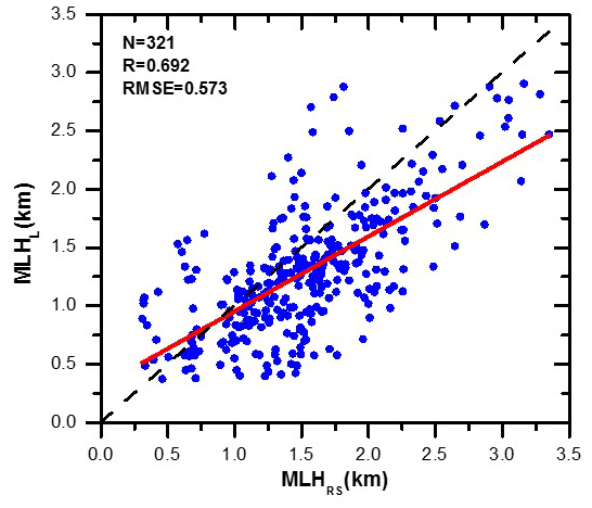
Figure 6 Comparisons between MLH_L in summer derived from lidar and MLH_RS from radiosonde at 14:00 (LST). The red line indicates the linear fitting of 321 samples, while the black dashed line represents the 1:1 line.

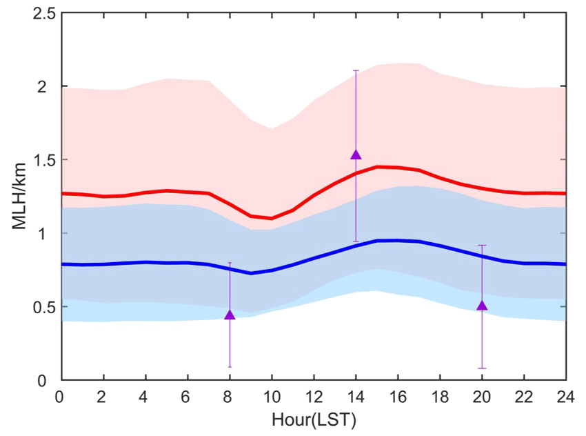
Figure 7 Diurnal cycles of the mixing layer height. The red line indicates the MLH_L retrieved from lidar, and the blue line represents the MLH${}_{\mathrm{L}}^{\prime }$ from lidar. The shaded areas show the standard deviation of MLH_L and MLH${}_{\mathrm{L}}^{\prime }$. Purple triangles indicate the MLH_RS averaged from routine RS data at 08:00 and 20:00 (LST) as well as from summer radiosonde at 14:00 (LST). The purple line indicates the standard deviation of MLH_RS.

The diurnal cycles derived from MLH_L match the RS results well in the afternoon, but they are larger than MLH_RS in the early morning and evening. Contrarily, MLH${}_{\mathrm{L}}^{\prime }$ tends to approach MLH_RS in the early morning and evening but stay far from MLH_RS in the afternoon. The difference between MLH_L (1.405±0.675 km, mean ± standard deviation of the mean) and MLH_RS (1.524±0.582 km) at 14:00 LST is around 0.120 km. This is reasonable considering that RS data are acquired at 14:00 LST only in summertime when MLH_L is usually larger throughout the year. However, the discrepancy between MLH${}_{\mathrm{L}}^{\prime }$ (0.912±0.315 km) and MLH_RS (1.524±0.582 km) at 1400 is around 0.612 km. Actually, MLH_L is nearly 0.46 km larger than MLH${}_{\mathrm{L}}^{\prime }$ throughout the day, with a bigger standard deviation. As for the measurement at 08:00 LST, the difference between MLH_L (1.196±0.710 km) and MLH_RS (0.434±0.364 km) is around 0.762 km, which is larger than the difference between MLH${}_{\mathrm{L}}^{\prime }$ (0.755±0.334 km) and MLH_RS (0.434±0.364 km). The discrepancy between lidar and RS measurements at 20:00 LST is similar.

Overall, MLH${}_{\mathrm{L}}^{\prime }$ can capture the high SBL height in the nocturnal time, when it is larger than 300 m. The stable layer height detected by MLH_L in the nighttime is the layer in which ground-emitted atmospheric pollutants are trapped; it contributes to the assessment of the surface pollutant concentration when there are emissions in the nocturnal time using numerical models (Collaud Coen et al., 2014). Due to incomplete optical overlap, in some cases the point derived from MLH${}_{\mathrm{L}}^{\prime }$ is the residual layer height rather than the low nocturnal SBL height. And in the daytime, MLH${}_{\mathrm{L}}^{\prime }$ tends to be lower than the CBL height. In the studies of Mues et al. (2017) and Kotthaus and Grimmond (2018), the MLH in the daytime is usually assigned as the lowest layer detected by a ceilometer. Using higher-power lasers (CE-370) with an increasing signal-to-noise ratio (SNR) and a small gradient detected, the attribution of the lowest layer in the daytime may remain open, since the first local maximum gradient (MLH${}_{\mathrm{L}}^{\prime }$) does not always correspond to the biggest local maximum (MLH_L). Our study indicates that MLH_L retrieves the consistent RL height during the night following the CBL diurnal maximal. The RL height corresponds to trapped atmospheric constituents discharged some hours before, which can be employed to convert column-mean optical depths into near-surface air quality information from remote sensing. And the SBL height provided by radiosonde at 08:00 and 20:00 LST can be considered complementary to the lidar approaches.

3.3 Climatology of MLH in Beijing

3.3.1 Seasonal variation

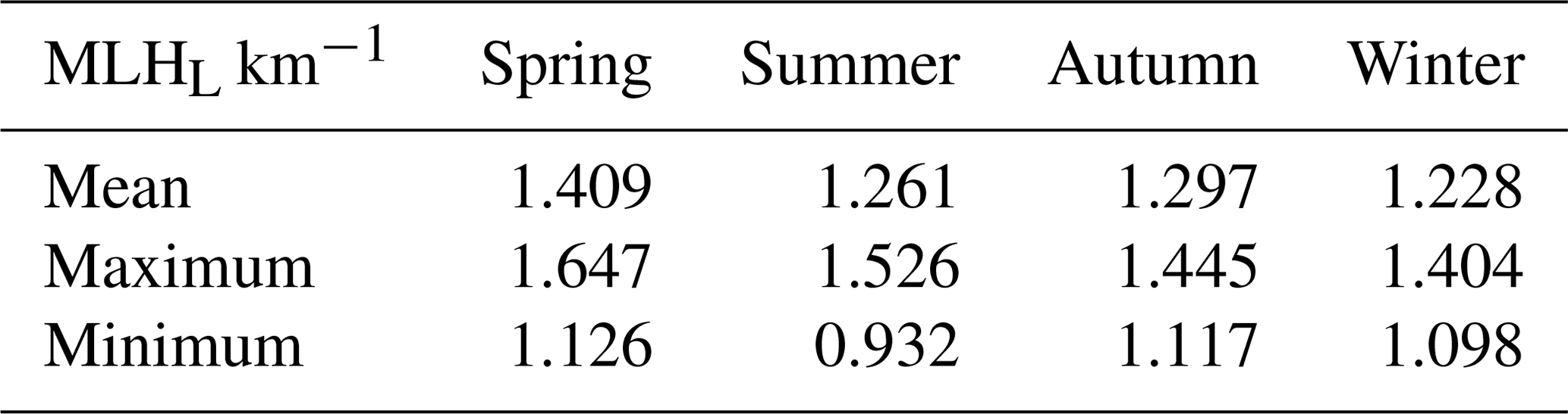
The seasonal mean diurnal cycle of the MLH_L from lidar is shown in Fig. 8. An evident seasonal variation in the magnitude of the diurnal cycle is observed. As shown in Table 1 and Fig. 8, the smallest MLH_L magnitude is found in winter, with the peak value of 1.404±0.751 km at 15:00 LST, whereas spring demonstrates the maximum magnitude with 1.647±0.754 km at 15:00 LST. The maximum in summer is 1.526±0.581 km, and the maximum in autumn is 1.445±0.837 km. From the all-day average of the four seasons, the averages in spring, summer, autumn and winter are 1.409, 1.261, 1.297 and 1.228 km, respectively. In summer, MLH_L acquired by lidar at 14:00 and 15:00 LST is 1.430 and 1.507 km, respectively, while MLH_RS at 14:00 LST is 1.524 km. The measurement of MLH_L at 15:00 LST is closer to MLH_RS at 14:00 LST. This is consistent with the case study in that it takes some time for aerosol to diffuse upward with the drive of thermal turbulence. As for the statistical variation, the values of autumn MLH_L vary most at each hour with the bigger standard deviation, indicating great fluctuations in the long measurement period, while the variation of summer MLH_L values for most hours is relatively stable.

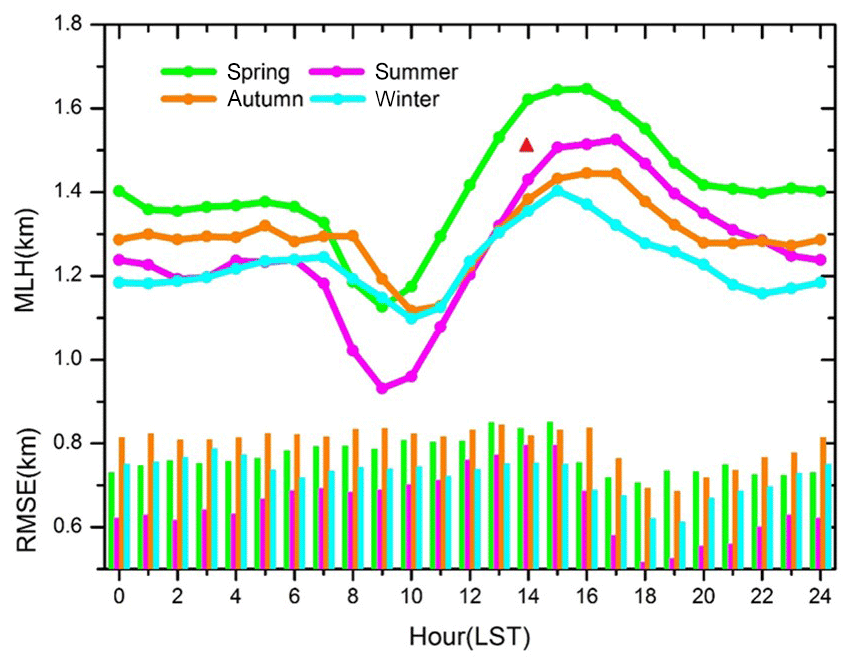
Figure 8 Seasonal variation of the diurnal cycles of MLH_L retrieved from lidar (dot lines) and the standard deviation of MLH_L (histograms). The red triangle indicates the MLH_RS measured at 14:00 LST by radiosonde.

Table 1 Statistics of boundary layer height seasonal change.

It should be noted that summer exhibits the biggest amplitude of the diurnal variation of MLH_L, with the deepest drop (0.93 km) increasing to the peak value of 1.51 km. Tang et al. (2016) indicate that the lower MLH_L value for summer nights and early mornings is attributed to effect of the mountain plain wind. When the local mountain breeze from the northeast in the summer night superimposes the surface cooling, leading to an increase in the thickness of the inversion layer, the height of the mixed layer gradually decreases. After sunrise, with the drive of thermal turbulence, the residual layer height observed by lidar is gradually replaced by a convective boundary layer height, with MLH_L increasing rapidly; after 12:00 LT, the plain wind from the southwesterly direction gradually dominates. Previous studies have suggested that the seasonal variation in the MLH_L may be associated with radiation flux (Stull, 1988; Kamp and McKendry, 2010; Munoz and Undurraga, 2010), which is consistent with our results. The observational data from Tang et al. (2016) indicate that radiation flux in spring is more than that in summer. The relatively low values in autumn and winter are likely related to the low radiation flux.

3.3.2 Interannual variation

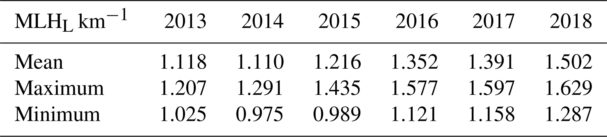
Interannual variations of the MLH_L diurnal cycle are investigated in Beijing from 2013 to 2018, as shown in Fig. 9. Diurnal variations of MLH_L in different years all have the same patterns but with a different magnitude. Clearly, from 2013 to 2018, the values of the diurnal circle of MLH_L increase year by year, including both the RL height at night and the CBL height in the daytime. Since the data for 2013 are mainly from winter and spring, the MLH_L seems stable, unlike the amplitude in other years. As shown in Fig. 9 and Table 2, from 2014 to 2018, the MLH_L all-day maximum values around 15:00 LST grow year by year, with values of 1.291±0.646 km, 1.435±0.755 km, 1.577±0.739 km, 1.597±0.701 km and 1.629±0.751 km, respectively. The all-day averages of MLH_L are 1.110, 1.216, 1.352, 1.391 and 1.502 km, respectively, also showing an increasing trend. This indicates that the volume available for the dispersion of pollutants is extending, which is beneficial to the mitigation of surface pollution. As shown in Fig. S5, from 2014 to 2018, the cumulative increase in the mean MLH_L for the whole day was 0.392 km, and the total increase in the maximum is 0.338 km. As for the annual increase in MLH_L, the average of the all-day increments in 2016 is the largest (0.136 km), while the average of the all-day increments in 2017 is the smallest (0.039 km).

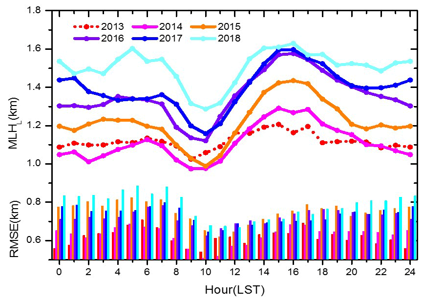
Figure 9 Interannual variation of the diurnal cycles of averaged MLH_L retrieved from lidar (dot lines) and the standard deviation of MLH_L (histograms). Due to the incomplete data for 2013, the MLH_L data for 2013 are presented as a dotted line.

Table 2 Statistics of boundary layer height interannual change.

In particular, the interannual variation of MLH_L in the period from 10:00 to 15:00 LST is calculated, when the PBL is characterized by an obvious convective boundary layer. From 2014 to 2018, the average CBL height shows a significant increasing trend of 1.075, 1.212, 1.324, 1.351 and 1.533 km, respectively. The total increase in the average CBL height is 0.458 km. As for the annual increase in CBL height, in 2018 it is the largest (0.182 km), while the average increment for the whole day in 2017 is the smallest (0.027 km).

It is found that, based on measurements from 2014 to 2017, MLH_L has a strong negative correlation with AOD ($R=-\mathrm{0.41}$) and with relative humidity ($R=-\mathrm{0.21}$), while MLH_L presents a positive correlation with wind speed (R=0.43) and shows no correlation with temperature (Fig. 10). As shown by the study of Wang et al. (2019), from 2014 to 2017 in Beijing, AOD and surface PM_2.5 have a tendency to decrease year by year, while MLH_L increases gradually. The reduction of AOD and surface PM_2.5 is revealed to relate to pollution emission control in recent years (Zhang et al., 2019). Compared with 2016, relative humidity increased in 2017 and wind speed weakened, which is not beneficial for the development of the MLH but is consistent with the small increase in MLH_L (0.027 km) in 2017. In addition to the effects of meteorological conditions, the increase in MLH_L benefits from the improvement of air quality in Beijing in recent years (Wang et al., 2019). Due to the scattering and absorbing of aerosol, solar radiation received from the ground decreases. It is thermal buoyancy generated from surface radiation that drives the PBL to develop. Thus, the development of the MLH is suppressed under a high aerosol load. Hence, with the relief of the radiation effect by aerosol during these years, the turbulence increases, thus leading to a larger PBL height (Ding et al., 2016; Li et al., 2017; Wang et al., 2019). The MLH affects the concentration of pollutants near the surface, while the total radiation of aerosol within the column atmosphere in turn influences the MLH.

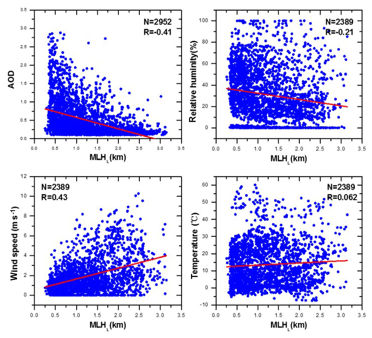
Figure 10 The correlation between MLH_L and AOD, relative humidity, wind speed and temperature for measurements from 2014 to 2017.

3.4 Implications for surface pollution retrieval

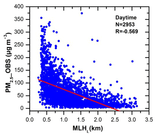
The vertical structure of the ML is important for pollution concentrations at the surface due to its impact on the volume into which pollutants are mixed (Miao et al., 2018). Mues et al. (2017) reported that black carbon concentrations show a clear anticorrelation with MLH measurements. Hu et al. (2014) found a negative correlation between near-surface O₃ and MLH for seven cities in the North China Plain. In the study, as shown in Fig. 11, the correlation between MLH_L and observed PM_2.5 data from the same observatory shows a high negative correlation ($R=-\mathrm{0.569}$) with 4 years of measurement (2014–2017). Actually, the pollutant concentration near the surface is affected by the overall effect of local emissions and meteorological conditions, with variation in different spatiotemporal distributions. The MLH is just one of these influencing factors. Geiß et al. (2017) indicated that when the MLH and near-surface concentrations are linked, it is necessary to take the locations and the details, i.e., meteorological conditions and local sources, of the MLH retrieval into account. In fact, all the data used in our study are from the same observatory. And the PMRS model used to calculate the surface PM_2.5 concentration includes the parameters for emissions (AOD) and meteorological conditions (RH).

Figure 11 The correlation between MLH_L and PM_2.5_OBS for measurements from 2014 to 2017.

Due to the difference in the sources of the MLH, lidar and radiosonde, the comparison of derived PM_2.5_lidar and PM_2.5_RS with in situ observational PM_2.5 data at 08:00 LST is presented in Fig. 12a and b. MLH from lidar shows reasonably good performance for the retrieval of PM_2.5 in the morning, with a correlation coefficient of 0.741 and RMSE 46.69 µg m⁻³. However, the calculated PM_2.5 from MLH_RS obviously overestimates the surface pollution, with lower correlation coefficients and a larger standard deviation. The large overestimation should be attributed to the underestimation of the aerosol layer height. In the morning when the PBL is not well developed, above MLH_RS there is still a large amount of aerosol, as seen in the lidar images in Figs. 1–4. The discrepancy makes sense given the method using the observed total amount of pollutant in the column atmosphere, including emissions from the surface and the residual aerosol from the day before. Therefore, MLH_L from lidar, as a good indicator of the aerosol layer height, is more suitable for estimating surface air pollution from column-mean optical depths.

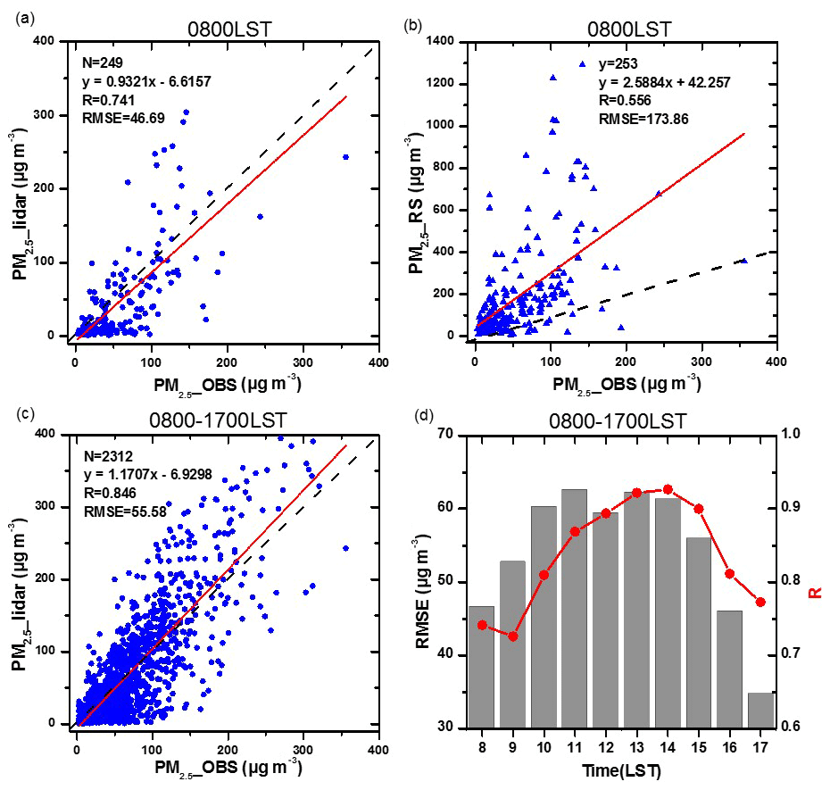
Figure 12 Comparisons between observed PM_2.5 and PM_2.5 calculated from the PMRS model using (a) MLH_L and (b) MLH_RS at 08:00 (LST) as well as (c) MLH_L for the period of 08:00–17:00 (LST). (d) The correlation coefficient and RMSE between observed PM_2.5 and PM_2.5 calculated from the PMRS model using MLH_L for each hour from 08:00 to 17:00 LST.

As presented in Fig. 12c, the calculated PM_2.5_lidar data for the daytime period (08:00–17:00 LST) show higher correlation (0.846) than those for only the early morning, and the slightly larger RMSE (55.58 µg m⁻³) is associated with the larger number of samples in the statistics. Considering the uncertainty of the series of parameters used in the model, the agreement between calculated PM_2.5_lidar and in situ measurements is reasonably good. Actually, the accuracy also shows a diurnal cycle, with the peak of correlation coefficients (0.927) at 14:00 LST (Fig. 12d). The correlations at 12:00, 13:00, 14:00 and 15:00 LST were 0.894, 0.922, 0.927 and 0.900, respectively. The higher accuracy may be due to the completed mixing of the aerosol at noon and the vertical distribution of the aerosol tending to be uniform. The correlation between 08:00, 09:00 and 17:00 LST is less than 0.8, which is related to the complex boundary layer structure in the morning and at nightfall. It is difficult to achieve full mixing of the aerosol in the stable boundary layer or the residual layer. The smaller RMSE is related to the limited number of samples. Therefore, the daily variation of the accuracy in the calculated surface pollutant using MLH retrieval by lidar varies with the daily variation of aerosol mixing uniformity at different times during the daytime. Based on the observational data, PM_2.5 tends to peak in the morning and evening. In contrast, afternoon usually witnessed lower mass concentrations due to the rapid vertical diffusion of aerosols (Guo et al., 2016, 2017). Thus, MLH_L from lidar can offer a significant contribution to retrieving the diurnal circle of surface air pollution.

4 Summary and conclusions

To acquire high-resolution observations of MLH diurnal variation, a study using lidar was performed from January 2013 to December 2018 in the Beijing urban area. The detection of the MLH based on two wavelet methods (MLH_L and MLH${}_{\mathrm{L}}^{\prime }$) applied to lidar observations was conducted. The two data results are compared with radiosonde as case studies and statistical forms. The temporal resolution (two or three measurements per day) of PBL detection by RS is not able to provide the mixing layer height diurnal cycle, regardless of its good precision. The MLH shows good performance for the convective layer height in the daytime and the residual layer height at night. MLH${}_{\mathrm{L}}^{\prime }$ has the potential to describe the stable layer height at night sometimes, even though the capability is limited due to the highly incomplete overlap with the lidar used in the study. The stable layer height detected by MLH${}_{\mathrm{L}}^{\prime }$ in the nighttime is the layer in which ground-emitted atmospheric pollutants are trapped; it contributes to the assessment of the surface pollutant concentration when there are emissions in the nocturnal time using numerical models. While the residual layer height corresponds to trapped atmospheric constituents discharged some hours before, it can be employed to convert column-mean optical depths into near-surface air quality information from remote sensing. And MLH${}_{\mathrm{L}}^{\prime }$ does not always capture the convective layer height as MLH_L in the afternoon. Nevertheless, MLH${}_{\mathrm{L}}^{\prime }$ could be useful as complementary information for the stable layer height in datasets of MLH_L.

A nearly 6-year climatology for the MLH_L diurnal cycle is calculated for convective and stable conditions. It is true that the height of the mixing layer obtained by different approaches may be different. We focus on the temporal change in the aerosol layer height with a consistent method using a dataset of MLH_L. The maximum MLH_L characteristics of seasonal change in Beijing indicate that it is low in winter (1.404±0.751 km) and autumn (1.445±0.837 km) and high in spring (1.647±0.754 km) and summer (1.526±0.581 km). A significant phenomenon is found from 2014 to 2018: the magnitude of the diurnal cycle of MLH_L increases year by year. The cumulative increase in the mean MLH_L for the whole day is 0.392 km, and the total increase in the maximum is 0.338 km. It may partly benefit from the improvement of air quality. As for converting the column optical depth to surface pollution, the calculated PM_2.5 using MLH_L data from lidar shows better accuracy than that from radiosonde compared with observational PM_2.5. Additionally, the accuracy of calculated PM_2.5 using MLH_L shows a diurnal cycle in the daytime, with the peak at 14:00 LST. For the operational measurement of PBL height, the MLH from lidar has the capability to mark the diurnal circle of the mixing layer height and can be used as an effective parameter for the vertical distribution of aerosols, providing an important reference to obtain near-ground pollutant concentrations with remote sensing.

Actually, interpreting data from aerosol lidar is often not straightforward because the detected aerosol layers are not always the result of ongoing vertical mixing; they may originate from advective transport or past accumulation processes (Russell et al., 1974; Coulter, 1979; Baxter, 1991; Batchvarova et al., 1999; Tang et al., 2016). Each detection method has good performances only for defined ML structures and under specific meteorological conditions. Therefore, the combination of several methods and instruments may contribute to characterizing the complete diurnal cycle of the complex ML structure (Wiegner et al., 2006; de Bruine et al., 2017; Morille et al., 2007; Kotthaus and Grimmond, 2018).