Observing carbon dioxide emissions over China's cities and industrial areas with the Orbiting Carbon Observatory-2

In order to track progress towards the global climate targets, the parties that signed the Paris Climate Agreement will regularly report their anthropogenic carbon dioxide (CO₂) emissions based on energy statistics and CO₂ emission factors. Independent evaluation of this self-reporting system is a fast-growing research topic. Here, we study the value of satellite observations of the column CO₂ concentrations to estimate CO₂ anthropogenic emissions with 5 years of the Orbiting Carbon Observatory-2 (OCO-2) retrievals over and around China. With the detailed information of emission source locations and the local wind, we successfully observe CO₂ plumes from 46 cities and industrial regions over China and quantify their CO₂ emissions from the OCO-2 observations, which add up to a total of 1.3 Gt CO₂ yr⁻¹ that accounts for approximately 13 % of mainland China's annual emissions. The number of cities whose emissions are constrained by OCO-2 here is 3 to 10 times larger than in previous studies that only focused on large cities and power plants in different locations around the world. Our satellite-based emission estimates are broadly consistent with the independent values from China's detailed emission inventory MEIC but are more different from those of two widely used global gridded emission datasets (i.e., EDGAR and ODIAC), especially for the emission estimates for the individual cities. These results demonstrate some skill in the satellite-based emission quantification for isolated source clusters with the OCO-2, despite the sparse sampling of this instrument not designed for this purpose. This skill can be improved by future satellite missions that will have a denser spatial sampling of surface emitting areas, which will come soon in the early 2020s.

1 Introduction

The Paris Agreement on climate change requires all parties (countries) to report their anthropogenic greenhouse gas emissions and removals at least every 2 years within an enhanced transparency framework (UNFCCC, 2018). Then, starting in 2023, the country reports will periodically form the basis for a global stocktake that will assess collective progress in bringing the global greenhouse gas emissions consistent with global warming well below 2 ^∘C above pre-industrial levels. In order to address potential biases in this self-reporting mechanism, the contribution of independent observation systems is being increasingly sought (IPCC, 2019). Our focus here is on the direct observation of fossil fuel carbon dioxide (CO₂) emission plumes from space and on the quantification of CO₂ emissions from this observation independently.

NASA's second Orbiting Carbon Observatory (OCO-2) polar satellite (Eldering et al., 2017) is one of the best existing instruments for the retrieval of column-averaged dry-air mole fraction of CO₂ (XCO₂). It observes the clear-sky and sunlit part of the Earth with footprints of a few square kilometers (1.29 km × 2.25 km) gathered in a ∼10 km wide swath for each orbit, particularly suitable for informing natural CO₂ budgets at the continental scale. It has already acquired more than 5 years of science data since its launch in July 2014, which have provided initial insight into carbon fluxes from the tropical terrestrial ecosystems (Liu et al., 2017; Palmer et al., 2019) but not without ambivalence due to likely significant residual systematic errors in the OCO-2 XCO₂ retrievals (Chevallier, 2018).

Extending the use of OCO-2 to monitor fossil fuel CO₂ emissions is rather challenging because the excess XCO₂ generated by large cities or power plants typically reaches ∼1 % at best (Kort et al., 2012), which is about 4 ppm compared with an instrument noise typically around 0.3–0.6 ppm (Worden et al., 2017) for a single sounding. This non-negligible noise in the XCO₂ retrievals is hardly balanced by the amount of data sampled near emission sources with a narrow swath, which hampers the detection of emission plumes and the precision of emission quantification. Only under rare occasions do the OCO-2 tracks cross CO₂ plumes downwind of large cities (Labzovskii et al., 2019; Reuter et al., 2019) or power plants (Schwandner et al., 2017; Nassar et al., 2017; Zheng et al., 2019), limiting the possibility to quantify the corresponding CO₂ emissions to a few cases within a year. So far, studies on the potential of spaceborne CO₂ observations to infer CO₂ emissions from large cities or power plants have relied on Observing System Simulation Experiments (OSSEs) (Bovensmann et al., 2010; O'Brien et al., 2016; Broquet et al., 2018; Kuhlmann et al., 2019; Wang et al., 2020) and on several well-chosen cases with real OCO-2 retrievals (Nassar et al., 2017; Reuter et al., 2019; Zheng et al., 2019; Wu et al., 2020). To our knowledge, no attempt has been made yet to infer anthropogenic emissions from actual OCO-2 data over a large area or a long period to evaluate a large-scale CO₂ budget.

Here we analyze all OCO-2 ground tracks between September 2014 and August 2019 over and around China, which is the largest emitter country in the world, in order to quantify CO₂ anthropogenic emissions at a large spatial extent over China. We develop a novel, simple, and effective approach to identify the CO₂ plumes from isolated emission clusters, to relate them unambiguously to nearby human emission sources, and to estimate the CO₂ emission fluxes causing each plume. The 5-year period allows nearly one-sixth of all the emissions from mainland China to be observed, although OCO-2 swaths have a low probability of crossing the emission plume from a given city. The budget of CO₂ emissions aggregating all the sources inferred from the satellite is compared to different emission inventories compiled by multiplying fuel consumption statistics by emission factors. Such a comparison, for the first time covering a significant fraction of the emissions from a country, demonstrates the potential of independently evaluating the self-reporting emission inventories from space.

2 Data and method

2.1 Data input

We use version 9r of the OCO-2 bias-corrected XCO₂ retrievals (Kiel et al., 2019). We use the good-quality data (xco2_quality_flag equals 0) over both land and ocean and associated retrieval uncertainty statistics. Our inversion framework relies on auxiliary information about winds and about the spatial distribution of emission sources, which are jointly used to link the observed CO₂ plume section with upwind local emission sources. We choose the spatially explicit Multi-resolution Emission Inventory for China (MEIC) dataset (Zheng et al., 2018a, b) that provides the locations of ∼100 000 individual industrial point sources (82 % of mainland China emissions) and $\mathrm{0.1}{}^{\circ }\times \mathrm{0.1}{}^{\circ }$ area source emissions (18 % of mainland China emissions) developed for the year 2013. Unlike other inventories used to map industrial emissions using spatial proxies, MEIC includes local reports from each power plant and industrial operator about their emissions and geographic locations. The ERA5 reanalysis data (C3S, 2017) provide us with a first guess for the local wind fields.

2.2 OCO-2 XCO₂ local enhancement

The key steps of our method are the identification of an XCO₂ local enhancement from the satellite data that can be attributed to a CO₂ plume from a large emission source, its separation from the surrounding background, and the establishment of a numerical link to the nearby upwind human emission sources. They are designed to account for the specificity of the sampling capability of OCO-2 and for the XCO₂ retrieval errors.

First, we look for XCO₂ anomalies along the OCO-2 tracks, which exceed 2σ of the spatial variability above the local average within 200 km wide moving windows centered on the locations of the anomalies. These anomalies potentially belong to significant CO₂ plumes. In each window corresponding to such an anomaly and with more than 200 high-quality retrievals (with ∼800 retrievals if none are missing due to cloud contaminations or other issues in the retrieval algorithm), the following curve fitting is applied to the XCO₂ retrieval data along the OCO-2 track:

$$\begin{array}{}\text{(1)}& y=m\cdot x+b+{\displaystyle \frac{A}{\mathit{\sigma }\sqrt{\mathrm{2}\mathit{\pi }}}}{e}^{\left[-{\left(x-\mathit{\mu }\right)}^{\mathrm{2}}/\mathrm{2}{\mathit{\sigma }}^{\mathrm{2}}\right]},\end{array}$$

where y is XCO₂ (ppm); x is the distance (km) along the OCO-2 track in a fitting window; and m, b, A, μ, and σ are parameters that determine the curve shape, estimated by a nonlinear least-squares fit weighted by the reciprocal of XCO₂ uncertainty statistics. The linear part $m\cdot x+b$ represents the background level assuming the background is linear (Reuter et al., 2019), while the remaining part depicts a single XCO₂ peak with a Gaussian shape (Nassar et al., 2017). Several XCO₂ anomalies should belong to the same CO₂ plume: in order to only define a single equation for a given plume and the corresponding background, we fit the curve around each XCO₂ anomaly and select the one with the largest R². We also reject all cases with low R² (less than 0.25) to achieve better fitting performance.

Second, we select the cases when the range of μ±3σis fully covered by the 200 km window to achieve complete fitting curves that cover both the plume part and the wide range of local background. To make the curve fitting robust, we further select the observational cases that have at least three valid cross-track footprints (eight footprints if none are missing) on average within the plume transect (μ±2σ) to constrain the shape of the fitted curve with enough data points. Finally, we check if the parameter A is positive and if the average XCO₂ value within the plume (defined as the average of raw XCO₂ retrievals within μ±2σ) minus the surrounding background concentration (derived as the average of raw XCO₂ retrievals outside 2σ) is larger than the standard deviation of the background values within 200 km. Only the cases that pass these two filtering criteria are finally identified as the XCO₂ local enhancements in this study.

2.3 Gaussian plume model

We use the Gaussian plume model (Bovensmann et al., 2010) to attribute the observed XCO₂ enhancement to a neighbor cluster of emission sources. We simulate the sum of XCO₂ plumes generated by each point source and each emission grid cell from the MEIC inventory within 50 km of the studied OCO-2 track with the equations

$$\begin{array}{}\text{(2)}& {\displaystyle }V=\sum _{\in \mathrm{50}\mathrm{km}}{\displaystyle \frac{F}{\sqrt{\mathrm{2}\mathit{\pi }}\cdot a\cdot z^{\mathrm{0.894}}\cdot u}}{e}^{-\frac{\mathrm{1}}{\mathrm{2}}{\left(\frac{n}{a\cdot z^{\mathrm{0.894}}}\right)}^{\mathrm{2}}},\text{(3)}& {\displaystyle }{\mathrm{XCO}}_{\mathrm{2}}=V\cdot {\displaystyle \frac{M_{\mathrm{air}}}{M_{{\mathrm{CO}}_{\mathrm{2}}}}}\cdot {\displaystyle \frac{g}{P_{\mathrm{surf}}-w\cdot g}}\cdot \mathrm{1000},\end{array}$$

where V is the CO₂ vertical column (g m⁻²) downwind of the emission sources, F is the emission rate (g s⁻¹), u is the wind speed (m s⁻¹), z is the along-wind distance (km), n is the across-wind distance (m), and a is the atmospheric stability parameter. Equation (3) converts V (g m⁻²) to XCO₂ (ppm), where M is the molecular weight (kg mol⁻¹), g is the gravitational acceleration (m s⁻²), P_surf is the surface pressure (Pa), and w is the total column water vapor (kg m⁻²).

F is derived from the MEIC emission inventory (Zheng et al., 2018b), including both point sources and $\mathrm{0.1}{}^{\circ }\times \mathrm{0.1}{}^{\circ }$ area source emissions. Each grid cell of area sources is used as a point source in Eq. (2). u is the average wind at 1000, 975, and 950 hPa to approximate the wind below 500 m (Beirle et al., 2011) at the time of the OCO-2 overpass, derived from the ERA5 reanalysis data (C3S, 2017). In the presence of relief, the average of the pressure-level winds is weighted towards the surface. a is a function of the atmospheric stability condition (Martin, 1976) determined by both the 10 m wind speed and the incoming solar radiation (Seinfeld and Pandis, 2006). Wind, solar radiation, and P_surf are all derived from the ERA5 reanalysis dataset (C3S, 2017), and w is adopted from the OCO-2 files.

2.4 Cross-sectional CO₂ flux estimate

We relate each satellite-observed XCO₂ enhancement to anthropogenic emission sources within 50 km using the Gaussian plume model. We visually inspect the observed and modeled XCO₂ and further select the ones that exhibit a single and isolated CO₂ plume to attribute the plume to a neighbor cluster of emission sources and estimate the corresponding cross-sectional CO₂ fluxes. We remove the linear background from the fitted curve of Eq. (1) and calculate the area under the remaining fitted curve to derive the CO₂ line density (ppm m), which can be converted to the unit of grams per meter through Eq. (3). The errors in the CO₂ line densities are those of the area under the fitted curve, mainly driven by the random errors of the XCO₂ retrievals and also by Eq. (1) that is not a perfect representation of actual CO₂ plumes. The standard error statistics for each parameter in Eq. (1) are obtained from the weighted nonlinear least-squares fitting and propagated to calculate the uncertainties of the area under the fitted curve.

The CO₂ line densities are multiplied by the wind speed (m s⁻¹) in the direction normal to the OCO-2 tracks at the location of the plume peak to estimate cross-sectional CO₂ fluxes (g s⁻¹). The average wind below 500 m is used like in Eq. (2). To reduce the errors in the wind direction, we allow rotation of the wind direction within 45^∘ on each side of the ERA5 local wind direction to maximize the spatial correlation between the Gaussian plume-modeled and the OCO-2-observed XCO₂ according to Nassar et al. (2017). The derived cross-sectional CO₂ fluxes approximately represent upwind source emissions under steady-state atmospheric conditions, while changes in the atmospheric stability (e.g., strong turbulent diffusion) could make the cross-sectional flux diverge from the source emissions (Varon et al., 2018; Reuter et al., 2019).

3 Results

3.1 CO₂ emission plumes seen by satellite

The identification of CO₂ emission plumes crossed by the satellite field of view starts with the search for XCO₂ local enhancements. These are defined as XCO₂ peaks above the background along the thin OCO-2 tracks. As shown in Fig. 1, we have identified a total of 6565 OCO-2 ground tracks over or around China between September 2014 and August 2019, with an even share between the cold-season (from September to February, 47 %) and the warm-season ones (from March to August, 53 %). We find 49 322 cases with local XCO₂ enhancements that exceed 2σ above the local average in a 200 km wide moving window along the satellite tracks. However, 97 % of these XCO₂ enhancements are removed after evaluation of the integrity of the plume section and of the spatial variation in surrounding background retrievals, leaving only 1439 XCO₂ cases as potent candidates for retrieving emissions.

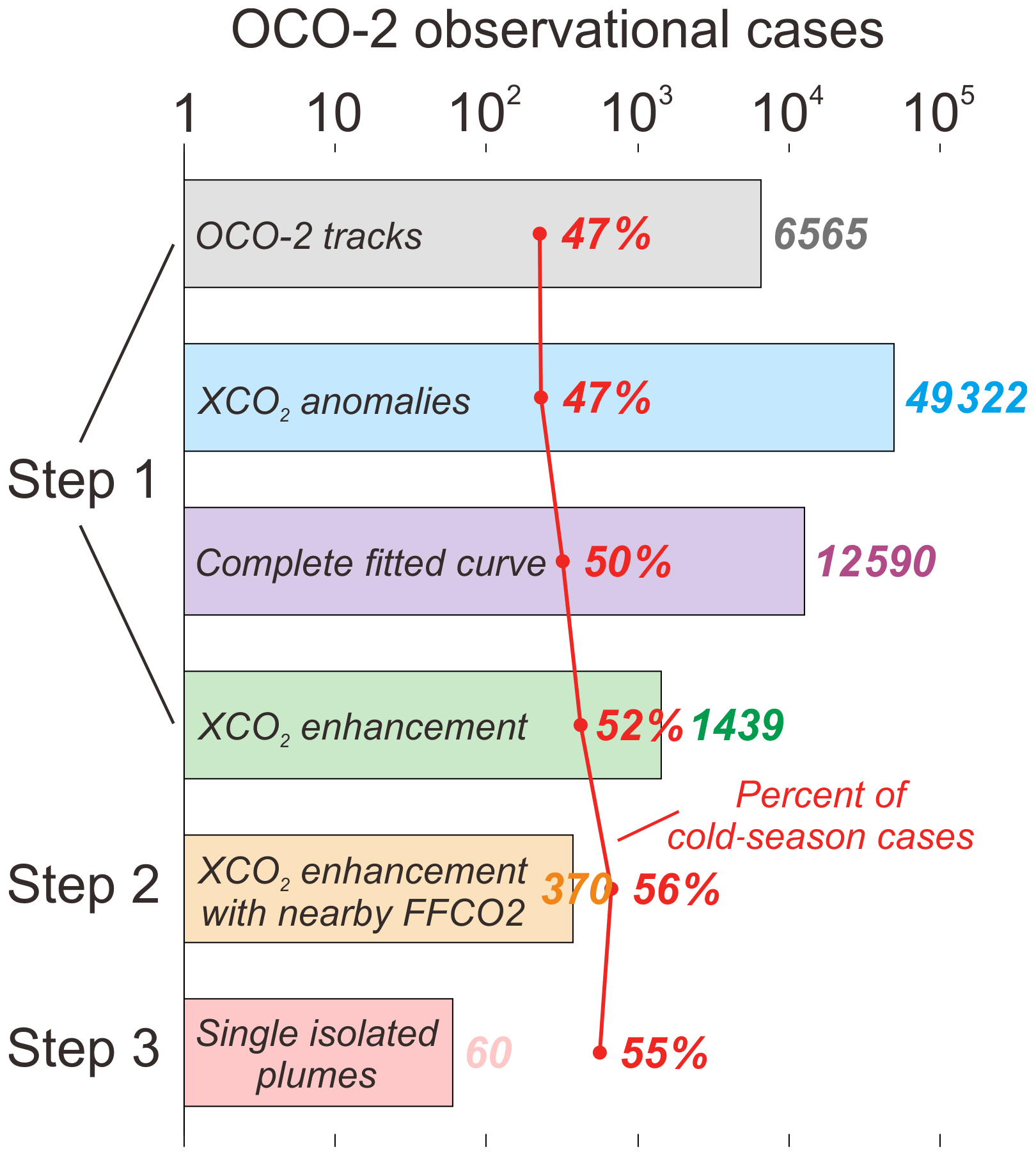
Figure 1 OCO-2 XCO₂ observational cases contained in each processing step. Step 1 starts from 6565 OCO-2 tracks around and over China between September 2014 and August 2019 (grey bar) and finds 49 322 XCO₂ anomalies along the OCO-2 tracks (blue bar). A total of 12 590 anomalies (purple bar) and their surrounding data points within a 200 km wide window can be fitted by a complete nonlinear curve using Eq. (1), of which 1439 XCO₂ anomalies (green bar) are identified as a local enhancement significantly higher than the background. Step 2 uses the Gaussian plume model to select 370 XCO₂ enhancements (yellow bar) that can be traced back to upwind fossil fuel emission sources within 50 km. In step 3, we finally select the 60 cases with single isolated CO₂ plumes to quantify the CO₂ emissions. The red curve shows the percentage of cold-season observational cases in each bar. The detail of each step is described in Sect. 2.

The second step consists in attempting to attribute the observed 1439 CO₂ enhancements to nearby human emission sources. Only 370 of the 1439 XCO₂ local enhancements can be related to emission sources in the MEIC dataset using the Gaussian plume model within a 50 km upwind distance from each OCO-2 ground track. The other cases that reveal XCO₂ enhancement but no nearby emission sources within 50 km upwind are probably due to either OCO-2 XCO₂ retrieval errors at local scales, sources missing in MEIC, or transport of CO₂ over a longer distance (Parazoo et al., 2011).

The third step is the quantification of cross-sectional CO₂ fluxes within the satellite-observed CO₂ plumes. Only 60 of the 370 cases correspond to single isolated CO₂ plumes within a 200 km wide window, which allows unambiguous attribution to an emission site or cluster. One reason why we reject the other 310 cases is that they have two or more individual plumes, partially overlapping or separated. Some of the rejected cases also lack observation data of good quality (xco2_quality_flag equals 0) at a distance of several tens of kilometers due to significant retrieval errors in the local satellite observations.

The data filtering process retains more cold-season observations (55 %) than warm-season ones, in particular after the first step (52 % cases are from the cold season after the first step), due to favorable meteorological patterns during the cold season. Although the total number of selected cases is small, it is several times larger than in previous studies that only focused on large cities and large power plants in different locations of the world (Nassar et al., 2017; Reuter et al., 2019; Wu et al., 2020). The finally selected 60 cases include both densely populated urban areas (33 cases) and small industrial areas (27 cases) that gather many industrial plants. The peak height of XCO₂ enhancement in the plumes ($A/\left(\mathit{\sigma }\sqrt{\mathrm{2}\mathit{\pi }}\right)$ in Eq. 1) is within 1.1–6.0 µmol mol⁻¹ (abbreviated as ppm) above the average local background and 2–7 times higher than the standard deviation of background levels within 200 km. The width of observed CO₂ plumes, defined as the full width at half maximum of peak height, is estimated between 2.2 and 61.2 km.

3.2 Quantifying CO₂ emissions: one city example

Figure 2 presents one example of the 60 selected cases. The emitter here is the city Anshan that has about 1.5 million inhabitants. On 17 October 2016, CO₂ emissions from Anshan were blown southward by a 7.1 m s⁻¹ wind at the OCO-2 overpass time and generated an XCO₂ local enhancement larger than 2 ppm (Fig. 2). At about 13:30 local time, OCO-2 flew over the east of China (Fig. 2a), crossed the CO₂ plume transported from Anshan, and successfully observed the local enhancement near the southernmost part of the OCO-2 ground track (Fig. 2b).

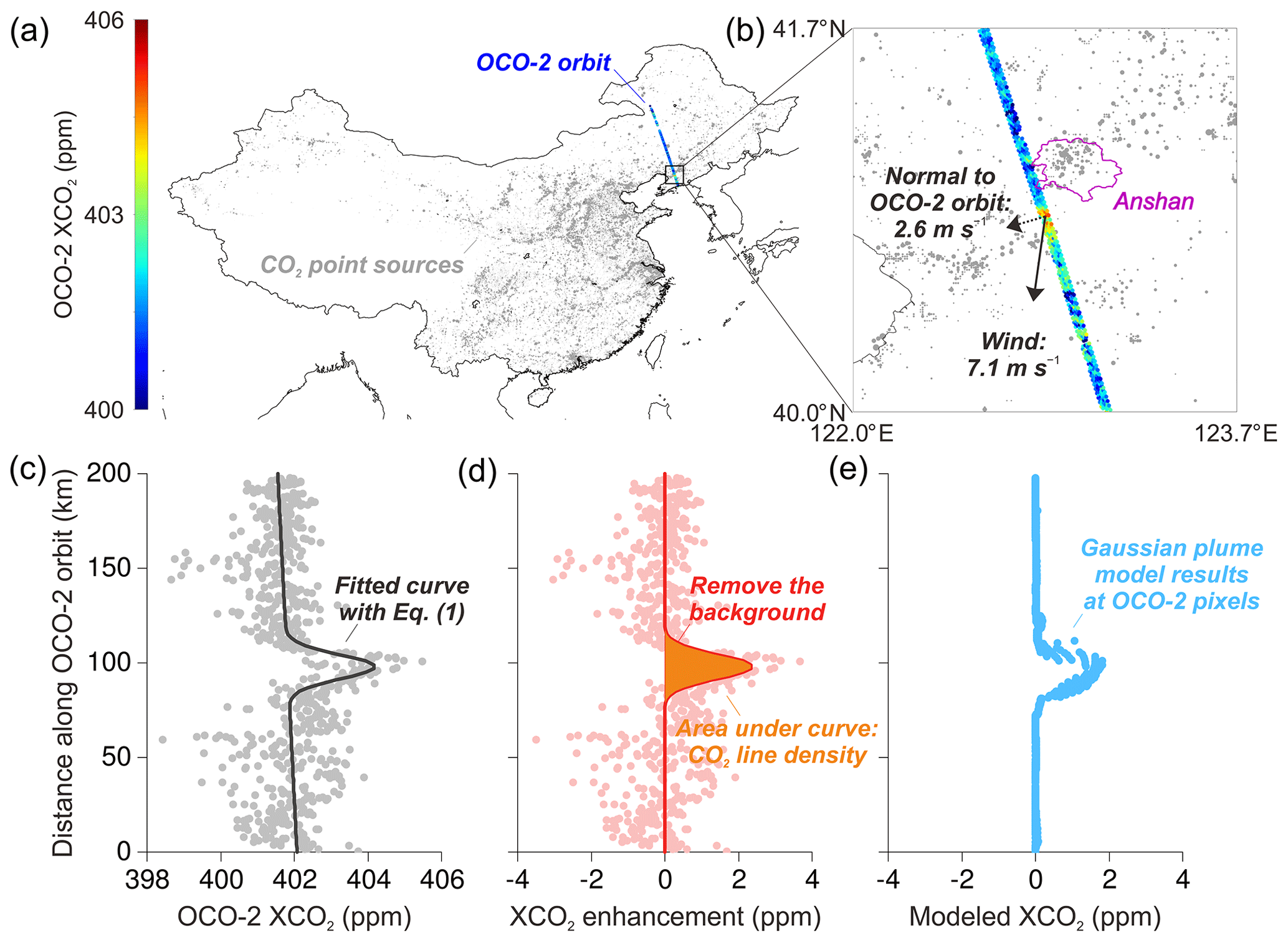
Figure 2 Quantification of CO₂ emissions from Anshan. (a) The OCO-2 orbit on 17 October 2016 is plotted on the map of MEIC emission point sources. (b) Zoom in closer to see OCO-2 XCO₂ data, local wind speed, and wind direction. The width of the track is made of eight cross-track OCO-2 footprints. (c) The valid XCO₂ data points (grey dots) plotted along the OCO-2 orbit with a fitted curve (black) based on Eq. (1). (d) The XCO₂ enhancement (red dots) above background, the fitted curve (red), and the area under the curve (orange shade). (e) The modeled XCO₂ enhancement (blue dots) by the Gaussian plume model combined with the MEIC emission inventory.

We plot the XCO₂ retrieval data (grey dots in Fig. 2c) along the satellite ground track, the plot window of which is centered at the highest XCO₂ value in the CO₂ plume. We first fit the black curve (R²=0.4) based on Eq. (1) to depict the CO₂ plume transect. The local background is represented by a straight line $-\mathrm{2.6}\times {\mathrm{10}}^{-\mathrm{3}}\cdot x+\mathrm{402.1}$ that approximates a flat background of 402.1 ppm. Then we subtract the background line from both the XCO₂ data and the fitted black curve to obtain the net enhancement of XCO₂ above the local background (pink dots and red curve in Fig. 2d). The maximum XCO₂ net enhancement (peak height of the red curve) is 2.4 ppm and the plume width is 15.0 km. The CO₂ line density is estimated as 0.60±0.04 t-CO₂ m⁻¹ (central estimate ±1σ) by computing the area under the red curve (the orange shade in Fig. 2d). The uncertainty is mainly caused by random errors of the single XCO₂ retrievals.

The CO₂ line density derived from the satellite retrievals is further multiplied by the wind speed in the normal direction to the OCO-2 track to quantify the cross-sectional CO₂ flux. We use the average wind below 500 m from the ERA5 reanalysis data. The ceiling height of 500 m is comparable to the maximum height that smoke plumes from power plants and industrial plants typically reach. The wind direction around Anshan is optimized according to Nassar et al. (2017) and is shifted by 1^∘ in this case to maximize the spatial correlation between the satellite-observed (Fig. 2d) and the model-simulated (Fig. 2e) XCO₂ enhancements. The wind speed in the normal direction to the OCO-2 track is then estimated as 2.6 m s⁻¹ at the location of the maximum XCO₂ value (Fig. 2b). The CO₂ hourly flux at the satellite overpassing time is finally estimated as 5.7±1.2 kt-CO₂ h⁻¹, considering uncertainties both in the CO₂ line density and in the wind speed.

The satellite-observed CO₂ plume can be traced back to anthropogenic emission sources located in the urbanized area of Anshan by the Gaussian plume model combined with the local emission map given by the MEIC inventory. We use monthly, weekly, and diurnal emission time profiles by region and by source sector from MEIC to split the annual emission totals reported by MEIC into hourly emission rates during the satellite overpass. The MEIC hourly emission rate of Anshan is 6.4±1.9 kt-CO₂ h⁻¹, which is close to the satellite-based inversion estimate.

3.3 CO₂ emission estimates for 60 cases in China

We quantify the CO₂ emissions corresponding to the 60 CO₂ plumes selected from the 5-year OCO-2 archive. These represent 46 different urban areas or industrial regions in China. There are 14 regions whose emission plumes were observed twice in our selection of the satellite data. The 60 CO₂ plumes present CO₂ line densities between 0.1 and 2.8 t-CO₂ m⁻¹, and hourly CO₂ fluxes at the time of the satellite overpass are estimated within the range of 0.3–16.0 kt-CO₂ h⁻¹ with the 1σ uncertainties of 20 %–30 %. The larger sources tend to present lower relative uncertainties, because a larger XCO₂ enhancement makes it easier to separate a plume from its background and is thus more easily observed by the satellite. The inversions that estimate CO₂ emissions larger than 4 kt-CO₂ h⁻¹ tend to constrain their relative uncertainties below 25 %.

We compare the satellite-based CO₂ hourly fluxes to the corresponding source emissions given by MEIC (Fig. 3), after applying emission time profiles to transform MEIC annual emissions into hourly emissions at the time of satellite overpass. Although the point-source-based MEIC emissions data are only for the year 2013, China's countrywide emissions remained stable between 2013 and 2017 and marginally grew only after 2017 (Friedlingstein et al., 2019). The satellite-based and MEIC-estimated emissions are broadly consistent within a factor of 2 (solid dots in Fig. 3) with comparable uncertainties for the same individual estimates. The average of satellite-based estimates is 27.1 % higher than the MEIC values in the cold season (solid blue dots in Fig. 3), while it is 5.2 % lower in the warm season (solid red dots in Fig. 3).

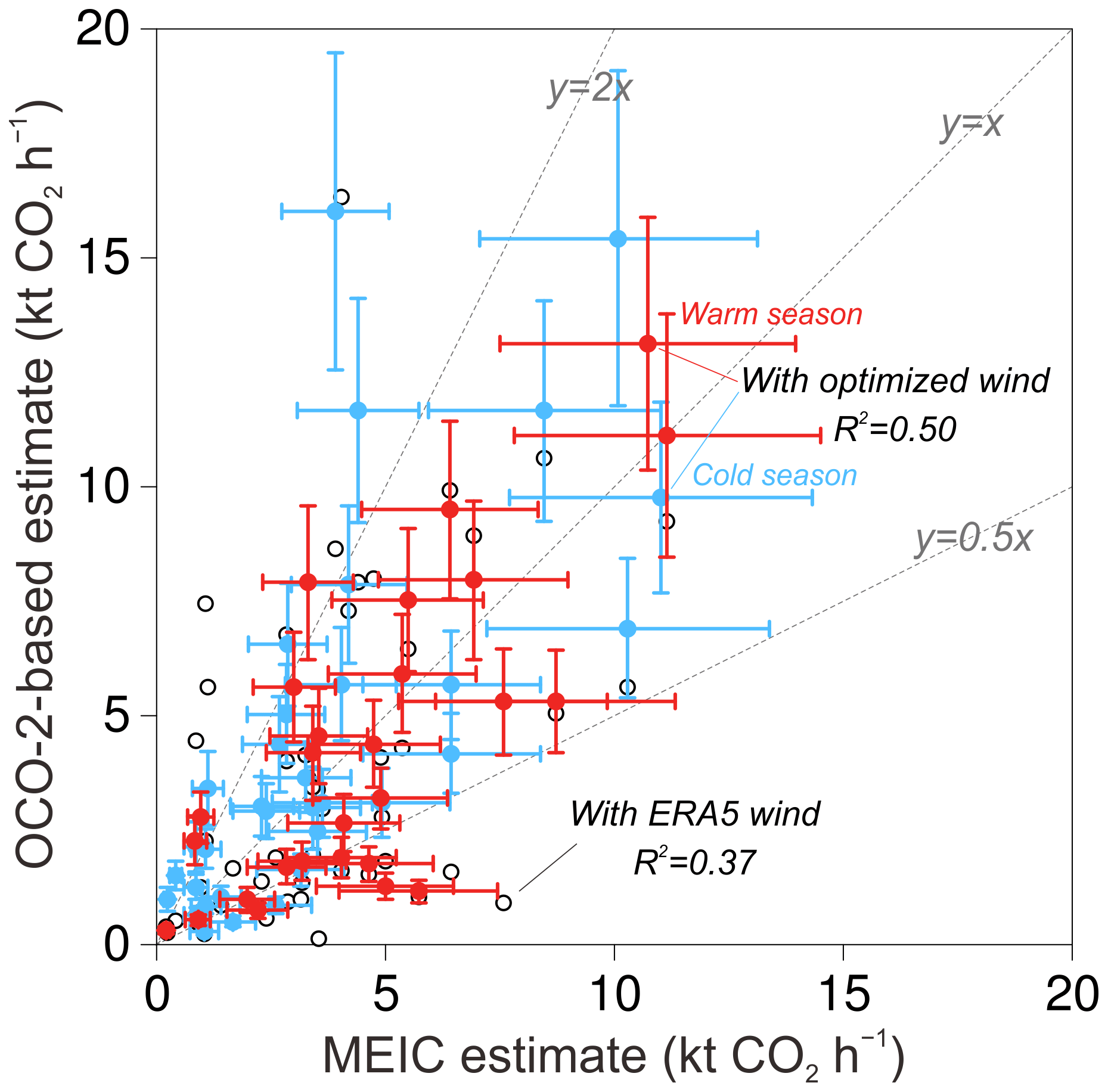
Figure 3 Comparison between OCO-2-based and MEIC-estimated CO₂ hourly fluxes. Each dot represents one of the 60 plume cases selected in this study, plotted according to the MEIC-estimated CO₂ flux (x axis) and the OCO-2-based estimate (y axis). The open dots are OCO-2 estimates using the ERA5 wind data, while the solid dots use the optimized wind and distinguish the warm-season (red dots) and the cold-season (blue dots) cases.

The differences in the results between cold and warm seasons could be due to uncertainties in the emission estimate methods of both our OCO-2-based inversion and the MEIC inventory. The larger satellite-based estimates in the cold season could be partially due to the fact that human respiration contributes to urban CO₂ fluxes while not included in the MEIC inventory of fossil fuel and cement emissions. We make a rough estimate of the metabolic CO₂ release by multiplying an emission factor of 0.52 t-CO₂ yr⁻¹ per person (Prairie and Duarte, 2007) by the population living in each emitting area. The results suggest that human metabolic CO₂ emissions explain 8 % of the larger satellite-based emission estimates on average in the cold season. The remaining difference could be due to the assumption that the 0–500 m average wind speed is representative of the transport wind in the plume diffusion, the natural processes like plant respiration, or the slight growth of fossil fuel emissions since 2013. However it could also reflect some bias in the MEIC estimates. In the warm season, despite human respiration emissions, the satellite-based inversions give lower emission estimates, possibly due to the carbon uptake by plants damping the XCO₂ enhancements (Mitchell et al., 2018), which makes anthropogenic emission signals not easily separated from the background in the satellite-based inversions.

The uncertainties in the satellite-based emission estimates are driven by those of the local wind field and of the CO₂ line density derived from the XCO₂ retrievals. We reduce the errors in wind directions and consequently increase the R² of the linear correlation between satellite- and MEIC-based emission estimates across emitting areas from 0.37 (open dots) to 0.50 (solid dots) as shown in Fig. 3. The magnitude of the wind speed uncertainty, typically considered 10 %–20 % (Nassar et al., 2017; Varon et al., 2018; Reuter et al., 2019), is comparable to the uncertainty in the satellite-based CO₂ line densities (3 %–23 % for the 60 emission plumes). In high-wind-speed conditions, the CO₂ plumes are spread more quickly and thus cause smaller local enhancements, which weakens the signal of XCO₂ and causes larger uncertainties in the estimate of CO₂ line densities. Generally, our estimates reach lower relative uncertainties for larger-emission cities under lower wind speeds.

3.4 Comparison with global bottom-up inventories

We extrapolate the satellite-based CO₂ hourly fluxes to annual total fluxes using emission time profiles, and we compare them to two global bottom-up emission maps: ODIAC (Oda and Maksyutov, 2015; Oda et al., 2018) and EDGAR (Janssens-Maenhout et al., 2019). We use the cases between the years 2014 and 2018 when both inventories are available, and we extract CO₂ emissions over each satellite-observed emitting area from the emission maps (Fig. 4). For the areas observed by the satellite in different years, we compute annual values from the corresponding inversions and average them for the comparison with ODIAC and EDGAR.

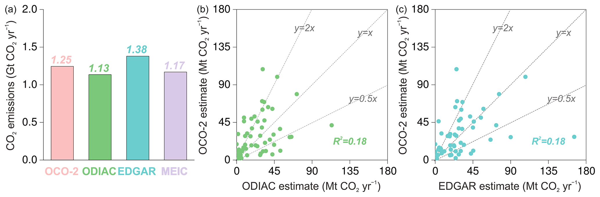
Figure 4 Comparing OCO-2-based CO₂ emission estimates with bottom-up inventories. (a) The sum of emissions from the different regions observed by OCO-2 between the years 2014 and 2018, including OCO-2 estimates (scaled up to annual emissions based on MEIC emission time profiles, pink bar), ODIAC (green bar), EDGAR (blue bar), and MEIC (purple bar) estimates. (b) Comparison of regional CO₂ emissions between OCO-2-based (y axis) and ODIAC estimates (x axis). (c) Comparison of regional CO₂ emissions between OCO-2-based (y axis) and EDGAR estimates (x axis).

For individual estimates, ODIAC (Fig. 4b) and EDGAR (Fig. 4c) are broadly consistent with the annual budgets from the satellite-based inversions, but the fit is slightly better in the case of EDGAR. The large discrepancies are not surprising since global emission inventories typically involve large uncertainties at city scales (Gately and Hutyra, 2017; Gurney et al., 2019), because they disaggregate national emissions to gridded maps with simple proxies like population or nighttime light in the countries like China where they lack detailed direct local information. Only large power plants have exact geographic locations (from the CARMA global database; Wheeler and Ummel, 2008), in principle, but not all of the industrial plants like MEIC. ODIAC uses nightlights to disaggregate national emission estimates to grid cells, which may lead to an underestimation of road emissions in cities (Gately and Hutyra, 2017) and a misplacing of industrial emissions. EDGAR relies on point source locations to allocate emissions in space while it still suffers from missing local information in China, and gridded population maps have to be used instead. Such an emission mapping approach overestimates emissions over densely populated cities in China (Zheng et al., 2017), because the industry plants, the primary CO₂ emission sources in China, are located far away from densely populated urban areas. The MEIC inventory estimates industrial emissions at the facility scale, transport emissions at the county scale, and residential emissions at the provincial scale, which can achieve better spatial accuracy in emissions estimates than the global emission inventories.

The sum of the emissions from the satellite-observed areas reaches 1.25 Gt CO₂ yr⁻¹ (Fig. 4a), accounting for approximately 13 % of the mainland China's total emissions. The corresponding bottom-up estimates from ODIAC, EDGAR, and MEIC are 1.13, 1.38, and 1.17 Gt CO₂ yr⁻¹, respectively. ODIAC emissions are 9.6 % lower than the satellite-based estimates while EDGAR emissions are 10.4 % higher. The slight growth of the emissions from 2014 to 2018 (documented in, e.g., EDGAR) could alone mostly explain the 6 % lower value for MEIC (valid for the year 2013) than the satellite estimate. Overall, EDGAR matches the individual estimates from the satellite-based inversions better than ODIAC for the 13 % of mainland China's CO₂ emissions that are observed by the satellite. However, both of these two global emission inventories reveal large uncertainties in emission estimates for individual areas as shown in Fig. 4b and c.

4 Conclusions

We developed a novel objective approach to quantify local anthropogenic CO₂ emissions from the OCO-2 XCO₂ satellite retrievals. The key of this method is a conservative selection of the satellite data that can be safely exploited for emission quantification. It also depends on the wind information and the information about the locations of human emission sources in the upwind vicinity of the selected OCO-2 tracks. Future developments could aim at refining the stringent data selection, or at improving the estimation of wind speed or the description of the plume footprint, for instance using detailed regional atmospheric transport models. However the current simplicity of our approach makes it easily applicable everywhere over the globe, in principle. Our first regional analysis over mainland China suggests that 13 % of its CO₂ human emissions can be observed and constrained, to some extent, by 5 years of retrieval data from the OCO-2, a satellite instrument not designed for this task. The satellite-based emission inversion results are broadly consistent (R²=0.50, meaning we agree on broad classes of emitters) with the reliable point-source-based MEIC regional inventory despite our simple modeling of the plume and of its background and despite possible biases due to local non-fossil-fuel emissions or local sinks that contribute to the plume intensity. We also use the satellite-based estimates as a rough independent evaluation of two global bottom-up inventories, ODIAC and EDGAR.

There is still a large gap between what the satellite can see and the National Greenhouse Gas Inventory reports submitted to the United Nations Framework Convention on Climate Change (UNFCCC), mentioned at the start of the introduction. The former is made of specific emission plumes linked to recent emission events without any sectoral distinction within the plume. The latter is made of the country- and annual-scale emission values assigned to specific human-caused source–sink categories. The exhaustiveness of the MEIC inventory, which involved detailed analysis of the fine spatial and temporal emission patterns, allowed us to bridge most of this gap for a time period when Chinese emissions did not vary much, but few countries have such a detailed geospatial inventory of their emissions and are able to update it timely for such a task. We also acknowledge the limitations of the temporal emission profiles even from the detailed MEIC inventory. The sparse sampling of the OCO-2 instrument, despite the good precision of individual soundings, will partly be overcome by the next generation of CO₂-dedicated imagery satellites, such as the CO₂ Monitoring mission (CO2M) in Europe (Clery, 2019; Janssens-Maenhout et al., 2020) and the Geostationary Carbon Cycle Observatory (GeoCarb) in the US (Moore et al., 2018) that will have denser spatial coverage. However, their measurement principle still relies on sunlight and will prevent us from sampling the diurnal emission cycle well. The need for a good knowledge of the emission space-time patterns (not only the emission values) will therefore remain for the comparison between the national inventories and the satellite-based estimates. However, for countries with less advanced CO₂ inventory infrastructures (typically non-Annex I parties to UNFCCC), we could also envisage an incremental approach where both bottom-up and top-down estimates are developed together in parallel.