Study of the dependence of long-term stratospheric ozone trends on local solar time

Reliable ozone trends after 2000 are essential to detect early ozone recovery. However, the long-term ground-based and satellite ozone profile trends reported in the literature show a high variability. There are multiple reasons for variability in the reported long-term trends such as the measurement timing and the dataset quality.

The Payerne Switzerland microwave radiometer (MWR) ozone trends are significantly positive at 2 % to 3 % per decade in the upper stratosphere (5–1 hPa, 35–48 km), with a high variation with altitude. This is in accordance with the Northern Hemisphere (NH) trends reported by other ground-based instruments in the SPARC LOTUS project. In order to determine what part of the variability between different datasets comes from measurement timing, Payerne MWR and SOCOL v3.0 chemistry–climate model (CCM) trends were estimated for each hour of the day with a multiple linear regression model. Trends were quantified as a function of local solar time (LST). In the middle and upper stratosphere, differences as a function of LST are reported for both the MWR and simulated trends for the post-2000 period. However, these differences are not significant at the 95 % confidence level. In the lower mesosphere (1–0.1 hPa, 48–65 km), the 2010–2018 day- and nighttime trends have been considered. Here again, the variation in the trend with LST is not significant at the 95 % confidence level. Based on these results we conclude that significant trend differences between instruments cannot be attributed to a systematic temporal sampling effect.

The dataset quality is of primary importance in a reliable trend derivation, and multi-instrument comparison analyses can be used to assess the long-term stability of data records by estimating the drift and bias of instruments. The Payerne MWR dataset has been homogenized to ensure a stable measurement contribution to the ozone profiles and to take into account the effects of three major instrument upgrades. At each instrument upgrade, a correction offset has been calculated using parallel measurements or simultaneous measurements by an independent instrument. At pressure levels smaller than 0.59 hPa (above ∼50 km), the homogenization corrections to be applied to the Payerne MWR ozone profiles are dependent on LST. Due to the lack of reference measurements with a comparable measurement contribution at a high time resolution, a comprehensive homogenization of the sub-daily ozone profiles was possible only for pressure levels larger than 0.59 hPa.

The ozone profile dataset from the Payerne MWR, Switzerland, was compared with profiles from the GROMOS MWR in Bern, Switzerland, satellite instruments (MLS, MIPAS, HALOE, SCHIAMACHY, GOMOS), and profiles simulated by the SOCOL v3.0 CCM. The long-term stability and mean biases of the time series were estimated as a function of the measurement time (day- and nighttime). The homogenized Payerne MWR ozone dataset agrees within ±5 % with the MLS dataset over the 30 to 65 km altitude range and within ±10 % of the HARMonized dataset of OZone profiles (HARMOZ, limb and occultation measurements from ENVISAT) over the 30 to 65 km altitude range. In the upper stratosphere, there is a large nighttime difference between Payerne MWR and other datasets, which is likely a result of the mesospheric signal aliasing with lower levels in the stratosphere due to a lower vertical resolution at that altitude. Hence, the induced bias at 55 km is considered an instrumental artifact and is not further analyzed.

1 Introduction

Since the discovery of the ozone hole over Antarctica in 1985 (Chubachi, 1985; Farman et al., 1985), the understanding of the mechanisms that drive stratospheric ozone trends has been a major area of interest in atmospheric research. After the first insights into the impacts of the Montreal Protocol on stratospheric ozone variability (Mäder et al., 2010, and references therein), the challenge is now to confirm the efficacy of the Montreal protocol by assessing stratospheric ozone recovery. Moreover, as ozone recovery is strongly influenced by climate change (Eyring et al., 2010; Meul et al., 2016), the continued monitoring of stratospheric ozone and its vertical structure is essential.

Chemical processes involved in polar ozone depletion also affect ozone in the stratosphere at a global scale (Solomon, 1999). In addition to the Chapman cycle, the main chemical species involved in stratospheric ozone loss processes are chlorine compounds (HCl, ClO_x), hydroxyl radicals (OH) and nitrogen oxides (NO_x), while stratospheric temperature (T) influences the rate of both ozone production and destruction. The effect of chlorine compounds on ozone loss has been extensively described in the literature (Farman et al., 1985; Solomon, 1999) since its first mention by Molina and Rowland (1974). In the stratosphere, the variability of NO_x plays a key role in the variability of ozone (Hendrick et al., 2012; Nedoluha et al., 2015a; Wang et al., 2014; Galytska et al., 2019), with an ozone conversion rate of the Chapman cycle of −0.25 ppmv h⁻¹ (Schanz et al., 2014). The NO_x catalytic cycle counteracts the accumulation of ozone during the day and leads to a negative correlation between anomalies in NO_x and the amplitude of the ozone diurnal cycle (Schanz et al., 2014). Finally, the negative correlation of ozone and temperature is mainly due to the temperature dependence of the rate coefficients of the Chapman cycle reactions (Barnett et al., 1975; Craig and Ohring, 1958).

In the mesosphere, OH radicals destroy ozone in auto-catalytic cycles and dominate the ozone budget above about 1 hPa (Lossow et al., 2019). Mesospheric OH is predominantly produced by the photodissociation of water vapor, and OH_x measurements can be used as a proxy for mesospheric H₂O (Newnham et al., 2019). The interaction of ozone with mesospheric water vapor is further described in Flury et al. (2009), Haefele et al. (2008) and references therein.

In the Northern Hemisphere (NH), upper-stratospheric ozone is reported to be increasing by 2 %–3 % per decade, due to both declining levels of ozone-depleting substances and stratospheric cooling. These estimates are based on measurements from satellites and ground-based instruments as well as chemistry–climate model simulations (Petropavlovskikh et al., 2019). This recovery is statistically significant down to 4 hPa (∼38 km); however, at altitudes below this level, NH midlatitude trends are not statistically significant. For the lowermost stratosphere, they even vary considerably between datasets (Bernet et al., 2019), although there is evidence for ongoing negative trends in some NH regions (Ball et al., 2018, 2019). For the mesosphere, negative trends have been reported in Moreira et al. (2015) and Kyrölä et al. (2013). In the Southern Hemisphere (SH) midlatitudes, satellites and ground-based datasets show statistically insignificant negative trends in the middle and lower stratosphere while upper-stratospheric trends are significantly positive at 2 % per decade mainly close to 2 hPa (Petropavlovskikh et al., 2019). In the tropics, a continuous decline in the middle and lower stratosphere is simulated by chemistry–climate models, and negative trends are retrieved from satellite and ground-based measurements (Petropavlovskikh et al., 2019) whose significance and magnitude are dataset dependent. The persistent negative trends are likely a consequence of dynamical forcing from climate change (Chipperfield et al., 2017). In the tropical upper-stratosphere trends are also positive, even if smaller than those in the midlatitudes.

Few studies report lower-mesospheric (altitudes above 0.6 hPa) ozone trends based on measurements for the period after 1998. Moreira et al. (2015) report negative trends up to −4 % per decade for the 1997–2015 period between 52 and 67 km in the NH. In Marsh et al. (2003), negative mesospheric long-term trends of −4 % per year are derived from HALOE sunset (SS) measurements before 2003.

Discrepancies between the post-1998 ozone profile trends calculated from ground-based instruments, satellite datasets and chemistry–climate models and the large uncertainties on the trends show that it is difficult to clearly provide evidence of stratospheric ozone recovery (Steinbrecht et al., 2017; Ball et al., 2017; Petropavlovskikh et al., 2019). In addition to information on the stability and drift of the measurements (Hubert et al., 2016), consideration of the ozone diurnal variability (Studer et al., 2014) and of the spatial and temporal sampling of the dataset (Damadeo et al., 2018) is of primary importance to understanding differences in the trends and to reduce the uncertainty associated with them. The variation in the trends with LST has to be quantified to calculate representative trends derived from sun-synchronous satellite measurements and ensure a proper comparison of these trends with those estimated from ground-based instruments, or to ensure a proper comparison of trends estimated from instruments with different measurement schedules. The consistent high time resolution of ground-based MWR instruments makes them ideal for analyzing this sampling bias.

In this study, we first carefully homogenize the SOMORA Payerne MWR ozone profile dataset and validate this dataset against simultaneous ozone profiles measured by satellites. We then investigate the effect of the ozone diurnal cycle on the linear trend after the year 2000 by calculating long-term trends for each hour of the day and night with a multiple linear regression (MLR) model. Finally we compare the SOMORA Payerne MWR ozone trends in the upper and middle stratosphere to trends of OH, NO_x and T derived from the SOCOL v3.0 CCM, to investigate the correlations between the long-term variability of ozone, water vapor, nitrous oxide and temperature, particularly at the diurnal scale.

The paper is organized as follows: Sect. 2 describes the ozone datasets measured by individual instruments. The homogenization of the Payerne MWR dataset is described in Sect. 3. Section 4 is dedicated to the description of the methods used to calculate the diurnal cycle and trends. In Sect. 5, we describe and discuss the results of the SOMORA Payerne MWR validation and of the dependence of the MLR trends as a function of the time of day. Conclusions about the variability of the long-term stratospheric ozone trends are provided in Sect. 6.

2 Data sources

2.1 Stratospheric Ozone MOnitoring RAdiometer (SOMORA)

The microwave radiometer SOMORA, hereafter referred to as the Payerne MWR, is located in Payerne (46.82^∘ N, 6.95^∘ E, 491 m), Switzerland, and has been operated continuously by MeteoSwiss since January 2000. Ozone profile retrievals are obtained independently of weather conditions throughout the diurnal cycle, forming a dataset with a constant and stable time sampling over 2 decades. Ozone profiles are provided in volume mixing ratio (ppmv) on a pressure grid between 47.3 and 0.05 hPa. The vertical resolution is 8–10 km from 47 to 1.8 hPa (20 to 40 km), increasing to 15–20 km at 0.18 hPa (60 km) (Maillard Barras et al., 2015). The measurement contribution is above 80 % from 47 to 0.27 hPa (20 to 57 km). The Payerne MWR is included in the Network for the Detection of Atmospheric Composition Change (NDACC).

2.1.1 Measurement principles and profile retrieval

Developed in 2000 by the University of Bern (Calisesi, 2000), the Payerne MWR is a total power microwave radiometer measuring the thermal emission line of ozone at 142.175 GHz. The electromagnetic radiation is measured at an antenna elevation angle of 39^∘, and the brightness temperatures range from 80 to 260 K. The Payerne MWR is calibrated using a hot load heated and stabilized at 300 K and a cold load at 77 K cooled with liquid nitrogen. A rotating planar mirror is used as a switch between the radiation sources. A Martin–Puplett interferometer (sideband filter) picks out the frequency band around 142 GHz. Outgoing from the front-end part (quasi optics), the signal is amplified and down-converted in frequency to 7.1 GHz (mixer) by means of a constant-frequency signal (GUNN oscillator). The signal is further down-converted in two steps (intermediate step at 1.5 GHz and 1 GHz) to the baseband (0–1 GHz). The spectral distribution, i.e., voltage as a function of channel or frequency, is measured by acousto-optical spectrometers (AOS) in the first decade and since then by an Acqiris fast-Fourier-transform spectrometer (FFTS) with 16 384 channels distributed over 1 GHz bandwidth.

The pressure broadening effect on the line allows the retrieval of the vertical ozone profile from the measured spectrum using an a priori profile, a radiative transfer simulation (forward model, ARTS; Buehler et al., 2005) and the optimal estimation method (OEM, Qpack; Eriksson et al., 2005) based on Rodgers (2000).

The required a priori information is taken from a monthly-varying climatology (called the ML climatology and described in McPeters and Labow (2012) formed by combining data from Aura MLS (2004–2010) with data from balloon radiosondes (1988–2010)). Ozone below 8 km is based on sonde measurements, from 16 to 65 km it is based on MLS measurements and above 65 km a climatological standard profile combining five satellite ozone datasets is used (described in Keating et al., 1990). Radiosonde and MLS data are blended in the tropospheric transition region. The ML climatology is combined with the Keating standard profile (Keating et al., 1990) in the mesospheric transition region.

The diagonal elements of the a priori covariance matrix are given by the variance of the ML climatology. The off-diagonal elements are parameterized with an exponentially decaying correlation function using a correlation length of 3 km. The diagonal elements of the error covariance matrix of the measured spectrum are estimated from the variance of the wings of the measured spectrum. The off-diagonal elements of the measurement error covariance matrix are zero.

The retrieval is characterized by the averaging kernel (AVK) matrix describing the changes in the retrieved profile as a function of changes in the true profile. The width of the AVKs is a measure of the vertical resolution of the retrievals, and the area of the AVKs indicates the measurement contribution to the retrieved profile (Rodgers, 2000). The ozone profile is considered reliable when the measurement contribution (MC) dominates the a priori information, i.e., when the measurement contribution is higher than 80 %. Figure 1 shows the Payerne MWR AVK means and the MC mean (×0.5) for one sample month (January 2013).

Figure 1 Mean values of Payerne MWR averaging kernels in parts per million per part per million and measurement contribution (×0.5) for January 2013. The shaded area represents the standard errors of the mean.

2.1.2 Data quality and reliability

The total uncertainty is calculated for each retrieved profile accounting for the following sources of uncertainty: measurement noise, tropospheric attenuation, calibration load temperatures, spectroscopy, atmospheric temperature profile and smoothing. The dominant source of uncertainty is smoothing because of the instrument's limited vertical resolution and is on the order of 15 %–20 % of the ozone content. The second most important contribution is the measurement noise on the spectra amounting to 3 %–7 % error when using a standard integration time of 1 h. Tropospheric attenuation correction, the pressure-broadening coefficient of the observed line, calibration load temperatures and the atmospheric temperature profile (Payerne radiosondes combined with the ECMWF ERA-Interim data) amount to an uncertainty of less than 3 %.

2.2 Other MWRs

2.2.1 GROMOS Bern microwave radiometer

The GROMOS (GROund-based Millimeter-wave Ozone Spectrometer) microwave radiometer, hereafter referred to as the Bern MWR, is a ground-based ozone microwave radiometer continuously observing the middle atmosphere above Bern (46.95^∘ N, 7.44^∘ E, 577 m), Switzerland, since November 1994. Like the Payerne MWR, the Bern MWR measures the thermal microwave emission of the rotational transition of ozone at 142.175 GHz, switching between the atmosphere, a cold load (liquid nitrogen at 80 K) and a hot load (electrical heater at 313 K). The Bern MWR spectral distribution has been measured since 1994 by a filter bank spectrometer with an integration time of 1 h (frequency resolution of 100 MHz to 200 kHz) replaced in 2009 by an FFTS with an integration time of 30 min (30.5 kHz frequency resolution). For technical details about the instrument, the measurement principle and the retrieval procedure, see Moreira et al. (2015) and Bernet et al. (2019, and references included therein). The vertical resolution is between 8 and 12 km in the stratosphere and increases with altitude to 20–25 km in the lower mesosphere. The measurement contribution is above 80 % from 20 to 52 km Moreira et al. (2015). The Bern MWR also contributes to NDACC.

2.2.2 Mauna Loa MWR

The Mauna Loa MWR (MLO MWR) operated by the US Naval Research Laboratory measures the emission spectrum of the ozone line at 110.836 GHz. It has been in operation at Mauna Loa (19.54^∘ N, 155.6^∘ W, 3397 m), USA, since 1995 and also contributes to NDACC. The spectral intensities are calibrated with black-body sources at ambient and liquid nitrogen temperatures. The experimental technique is described in Parrish et al. (1992), and technical details about the instrument are provided in Parrish (1994). While the basic radiometric features are similar to the Bern and Payerne MWRs, the MLO MWR receiver is cryogenically cooled, and the spectral distribution is measured by a filter bank spectrometer. The ozone mixing ratio profiles are retrieved from the spectra using an adaptation of the optimal estimation method of Rodgers (Connor et al., 1995; Rodgers, 2000).

The vertical resolution is 6 km at an altitude of 32 km, between 6 and 8 km from 20 to 42 km, and then increases to 14 km at 65 km. The measurement contribution is above 80 % from 20 to 70 km. While hourly measurements are performed for the purpose of diurnal cycle studies (Parrish et al., 2014), data are deposited in the NDACC with a 6-hourly time resolution. The NDACC dataset is used in this study. The MLO MWR underwent a major spectrometer upgrade between 2015 and 2017. For this study, only data until May 2015 have been used.

2.3 Satellites

The Payerne MWR is compared to the three instruments from the ENVISAT satellite: GOMOS (Global Ozone Monitoring by Occultation of Stars), MIPAS (Michelson Interferometer for Passive Atmospheric Sounding) and SCIAMACHY (SCanning Imaging Absorption spectroMeter for Atmospheric CHartographY), as well as to the MLS (Microwave Limb Sounder) on the Aura satellite and HALOE (Halogen Occultation Experiment) on the UARS satellite. The ENVISAT instruments are part of the Ozone Climate Change Initiative (Ozone CCI).

The HARMOZ dataset (Sofieva et al., 2013) is based on limb and occultation measurements from ENVISAT (GOMOS, MIPAS and SCIAMACHY), Odin (OSIRIS, SMR) and SCISAT (ACE-FTS) satellite instruments providing ozone profiles in the altitude range from the upper troposphere up to the mesosphere in the years 2001–2012. The ozone profiles are given in number density on a common pressure grid, which corresponds to a vertical sampling of 2–3 km.

HARMOZ and HALOE data centered 10^∘ by 10^∘ around Payerne were selected (equivalent to an area of approximately 1110 km by 760 km). The collocation criterion for MLS satellite data is $\pm \mathrm{3}{}^{\circ }$ in latitude and $\pm \mathrm{5}{}^{\circ }$ in longitude (an area of approximately 666 km by 760 km). This criterion ensures a sufficient number of collocated measurements and thus provides reliable bias estimates.

2.3.1 MLS

MLS is a microwave limb-sounding radiometer on board the Aura Earth observing satellite. Ozone profiles are retrieved from MLS radiance measurements at 240 GHz. Details about the Aura mission can be found in Waters et al. (2006). In this study we use ozone profiles from the version 4.2 dataset (Livesey, 2018). MLS measures ozone profiles from 10 to 75 km with the vertical resolution ranging from 2.5 to 4 km. MLS passes over Payerne at 01:30 and 13:30 UTC. For the comparison with coincident Payerne MWR ozone profiles, the MLS profiles are convolved to the Payerne MWR vertical resolution using AVKs.

2.3.2 ENVISAT

MIPAS is an infrared limb emission Fourier-transform spectrometer (spectral range from 685 to 2410 cm⁻¹) on board the ENVISAT satellite. MIPAS provided profiles of H₂O, O₃, HNO₃, CH₄, N₂O and NO₂ from 2002 to 2012. Stratospheric ozone profiles are retrieved with the version V7R_O3_240 research processor developed at KIT IMK/IAA via constrained inverse modeling of limb radiances (Laeng et al., 2017). Data used in this study are the OR (Optimized Resolution) dataset from 2005 to 2012. MIPAS measured ozone profiles from 10 to 80 km, with a vertical resolution ranging from 2.4 km at an altitude of 10 to 3.6 km at 30 and 5 km at 70 km.

GOMOS was a stellar occultation instrument on board ENVISAT from 2002 to 2012 (Bertaux et al., 2010). GBL (Gomos Bright Light) measured the atmospheric limb radiance of scattered sunlight (Tukiainen et al., 2015). Ozone profiles are retrieved using the ESA IPF v6 processor (Sofieva et al., 2017) from the ultraviolet and visible spectrometer measurements at wavelengths between 250 and 692 nm with a two-step inversion (Kyrölä et al., 2010). ENVISAT overpass times for Payerne are 10:00 UTC (GBL dataset) and 22:00 UTC (GOMOS dataset). GOMOS measured ozone profiles from 20 to 100 km, with a vertical resolution of 2 km below altitudes of 30 km and 3 km above 40 km.

SCIAMACHY was a spaceborne spectrometer that measured the upwelling radiation from the Earth's atmosphere in the UV, visible, near-infrared and shortwave-infrared spectral ranges. A detailed description of the instrument and its measurement modes can be found in Bovensmann et al. (1999). Ozone profiles used in this study are retrieved using the University of Bremen (UBR) limb retrieval algorithm (V3_5). SCIAMACHY measured ozone profiles from 15 to 40 km, with a vertical resolution of 3 km. While measuring, SCIAMACHY passed over Payerne at 10:00 UTC. The MIPAS, GOMOS, GBL and SCIAMACHY profiles are AVK-convolved to the vertical resolution of the Payerne MWR, and conversion from number density (HARMOZ dataset) to parts per million is carried out using ECMWF temperature profiles as a common auxiliary temperature profile. The auxiliary pressure and temperature profiles used for the unit conversion and for the vertical coordinate change influence the satellites' ozone profile difference as pointed out in Hubert et al. (2016).

2.3.3 HALOE

HALOE was a mid-infrared solar occultation instrument on board the UARS (Upper Atmosphere Research Satellite) from 1991 to 2005 (Russell et al., 1993). HALOE retrieved vertical profiles of O₃, HCl, HF, CH₄, H₂O, NO, NO₂, aerosols and temperature from 15 daily sunrise (SR) and sunset (SS) measurements equally spaced in longitude. Data used in this study are the third public release record (v19). HALOE measured ozone profiles from 15 to 80 km with a vertical resolution of 3–5 km. For comparison with coincident Payerne MWR ozone profiles, the HALOE profiles are AVK-convolved to the Payerne MWR vertical resolution.

2.4 SOCOL CCM

The SOlar Climate Ozone Links (SOCOL) CCM consists of the middle-atmosphere version of the MA-ECHAM general circulation model (Roeckner et al., 2003; Giorgetta et al., 2006), with 39 vertical levels between the surface and 0.01 hPa (∼80 km) coupled to the Model for Evaluation of oZONe trends (MEZON) chemistry module (Egorova et al., 2003). Dynamical and physical processes in the CCM SOCOL are calculated every 15 min within the model, while full radiative and chemical calculations are performed every 2 h. Chemical constituents are transported using a flux-form semi-Lagrangian scheme (Lin and Rood, 1996). The original version includes 41 chemical species participating in 140 gas-phase, 46 photolysis and 16 heterogeneous reactions. The CCM SOCOL exploits T42 horizontal spectral truncation, which corresponds approximately to 2.5^∘ by 2.5^∘ resolution. The first model version was described and evaluated by Stenke et al. (2013). The model now includes an isoprene oxidation mechanism (Poeschl et al., 2000), the online calculation of lightning NO_x emissions (Price and Rind, 1992), treatment of the effects produced by different energetic particles (Rozanov et al., 2012), updated reaction rates and absorption cross sections (Sander, 2011), improved solar heating rates (Sukhodolov et al., 2014), and a parameterization of cloud effects on photolysis rates (Chang et al., 1987). All considered halogenated ozone-depleting species are transported as separate tracers.

The SOCOL v3.0 dataset has been validated in the troposphere and stratosphere with satellites, NDACC ground-based instruments and other CCMs (Staehelin et al., 2017; Revell et al., 2015; Stenke et al., 2013). Stratospheric ozone trends derived from SOCOL v3.0 in specified dynamics mode have also been compared with trends derived from measurements (Ball et al., 2018). For the comparison with ground-based observations the model outputs were horizontally interpolated to the location of Payerne from the adjacent grid cells. An AVK convolution was also applied to the model data for comparison with the Payerne MWR profiles.

3 Homogenization of the Payerne MWR dataset

The homogenization of the Payerne MWR dataset was performed in stages. First, the integration time has been adapted at each upgrade transition to ensure a constant measurement contribution over the dataset time range. At the spectrometer upgrade transition (AOS to FFTS), a correction offset has been calculated over 1 year of simultaneous measurements. At the front end and the GUNN oscillator upgrade transitions, the correction offsets have been calculated using simultaneous measurements by an independent instrument, by the Bern MWR and by the MLS satellite. Moreover, the homogenization corrections to be applied to the Payerne MWR ozone profiles are dependent on local solar time (LST).

3.1 Homogenization of the Payerne MWR AOS and FFTS time series

Spectral analysis of the Payerne MWR measurements was performed using two acousto-optical spectrometers (AOSs) from January 2000 to October 2010; the AOS had a total bandwidth of 1 GHz, with a frequency resolution varying from 24 kHz at the line center to 980 kHz at the wings. In September 2009, an Acqiris FFTS spectrometer was added as a back end to the Payerne MWR. The FFTS covers a total bandwidth of 1 GHz with 16 384 channels, providing a frequency resolution of 61 kHz. This technical upgrade introduced a discontinuity in the time series, requiring a homogenization of the dataset. The AOS and FFTS were used in parallel for 1 year to ensure a proper homogenization of the transition.

The measurement contributions to simultaneous ozone profiles retrieved from the AOS and FFTS measurements were compared for the overlap period of 1 year and found to be different when considering the same integration time (not shown). In order to assess the influence of such a difference on the ozone content, the monthly means of the measurement contribution at 0.4 hPa as a percentage of the ozone profile are plotted in Fig. 2 against the monthly means of the diurnal cycle amplitude (maximum-to-minimum difference) as a percentage of the midnight ozone value for the 2000–2016 measurement period. A clear negative correlation between the amplitude of the ozone diurnal cycle and the measurement contribution is shown for the lower mesosphere. A low measurement contribution means there is a large a priori contribution. Since the a priori profile is a standard climatological ozone profile without any diurnal variation, the lower the measurement contribution, the lower the diurnal cycle amplitude. Since the ozone diurnal cycle amplitude is correlated to the measurement contribution value, a proper homogenization should not be limited to a correction of the bias between profiles retrieved from the spectra measured by the two spectral setups but should include a full homogenization of the characteristics of the retrieval (measurement response and vertical resolution). The AOS and FFTS ozone profile datasets used in this study were harmonized by ensuring a constant measurement contribution in time to each layer of the retrieved ozone profiles between 47 and 0.05 hPa (20 and 70 km). The integration time for one ozone profile therefore varies from 30 min to 2 h. For a stable measurement contribution over the AOS to FFTS transition in the upper stratosphere–lower mesosphere, FFTS measurements require being accumulated over 2 h (FFTS2h dataset). However, in the altitude range where the measurement contribution is much larger than 80 %, a FFTS signal accumulation time of 1 h is sufficient, therefore allowing a higher-time-resolution dataset (FFTS1h dataset). The FFTS1h data are used for the middle stratosphere and upper stratosphere below 48 km where high time resolution without any degradation of the measurement contribution is required. The FFTS2h data are used for the lower mesosphere where the consistency of the measurement contribution is more important than the time resolution requirement.

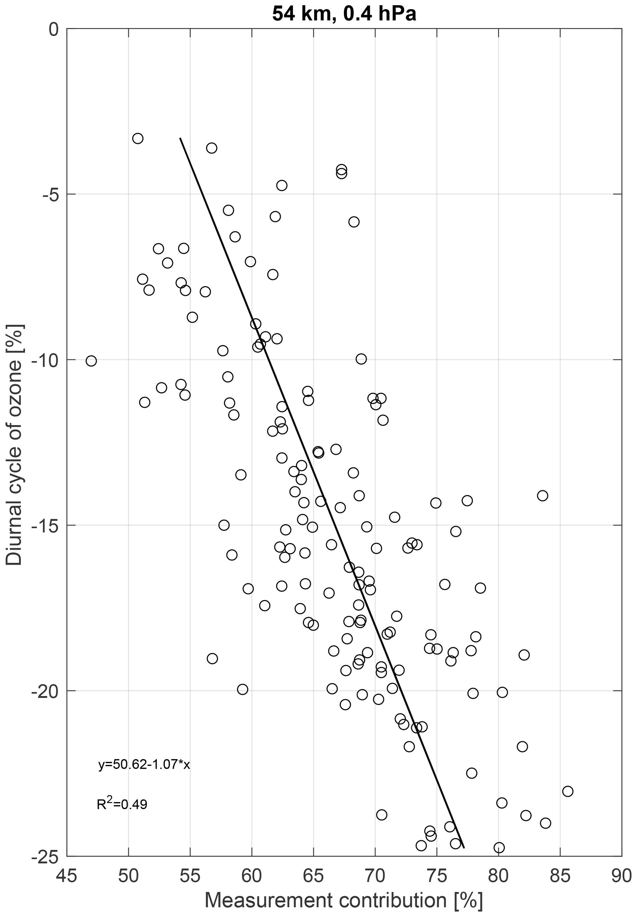
Figure 2 Ozone diurnal cycle amplitude (in percent of midnight value) as a function of measurement contribution (in percent of ozone content) for the lower mesosphere (0.4 hPa).

The bias between the profiles retrieved from the two spectral measurement setups was then determined from monthly means of simultaneous measurements during the 1 year transition period. The mean absolute difference for each profile layer was subtracted from the aggregated AOS profiles, keeping the FFTS profile dataset unchanged. The bias correction values have been determined for each pressure level and respectively applied to each pressure level. Bias values are within 10 % between 47 and 0.05 hPa (20 to 70 km).

The application range of the correction offset depends to a large extent on the way the offset is calculated. The AOS to FFTS correction offset, when determined by the comparison of simultaneous monthly means, should be applied only to the global monthly mean time series and not to sub-daily monthly means. In addition to the pressure level dependence, the time dependence (LST dependence) of the correction factor has been determined for the AOS-to-FFTS transition (for both the 1 and 2 h bins) using monthly means of simultaneous Payerne and Bern MWRs measurements. As shown in Fig. 3a and b, the correction offsets do not vary significantly with LST below 50 km (0.6 hPa). No LST-dependent correction factor has then been applied to the monthly mean time series in the stratosphere. However, in the lower mesosphere, the AOS-to-FFTS 2 h correction offset is lower during daytime than during nighttime, following the diurnal variation in ozone. A correction offset depending on the LST has to be applied to the AOS data above 50 km for a proper homogenization of time series when LST-dependent monthly means are considered. The AOS-to-FFTS spectrometer upgrade influences the measurement contribution function of the ozone profile in a nonlinear way. The resulting offset will depend on the altitude and on the amount of ozone. As above 50 km, the ozone intensity varies with LST (diurnal cycle up to 25 %), the offset presents a similar behavior.

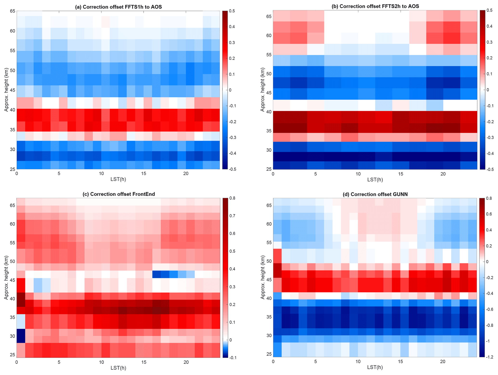
Figure 3 (a, b) Payerne MWR AOS setup vs. FFT setup offset profiles in parts per million as a function of LST; (c) correction offset for the front end (in 2005) and (d) for the GUNN oscillator (in 2009) technical upgrades.

3.2 Time series corrections for technical issues

Since January 2000 the Payerne MWR has been affected by several technical issues: the mixer diode was replaced in 2001, the front end was changed in 2005 and the GUNN oscillator was repaired in 2009. Each of these major technical interventions could potentially affect the measured spectrum by modifying the baseline shape and the receiver temperature. The retrieval was adapted between the 2001 and 2005 interventions by considering a sinusoidal function in the spectrum background removal. For the correction of the effects from the 2005 and 2009 interventions, homogenization of the ozone profile time series was performed using coincident AVK convolved ozone profiles from the Bern MWR and Aura MLS. The absolute mean differences of the coincident datasets were considered. For the 2005 homogenization, the difference between the Payerne MWR AOS dataset and the Bern MWR after the upgrade (in 2007, since in 2006 the Bern MWR dataset presents a negative anomaly compared to other instruments; Bernet et al., 2019) was subtracted from the difference between the Payerne MWR AOS dataset and the Bern MWR before the upgrade (in 2004). This relative bias was then removed from the Payerne MWR profile dataset prior to the 2005 intervention. For the 2009 homogenization, the difference between the Payerne MWR AOS dataset and MLS in 2010 was subtracted from the difference between the Payerne MWR AOS dataset and MLS in 2008. This relative bias was then removed from the Payerne MWR profile dataset prior to the 2009 intervention. These homogenizations are only possible if it is assumed the reference instruments (i.e., the Bern MWR and MLS) do not drift during the periods considered. The Bern MWR dataset does not present any anomalies compared to other ground-based instruments in 2004 and 2007 (Bernet et al., 2019), and the MLS dataset does not present any anomalies compared to other satellite instruments between 2008 and 2010 (Hubert et al., 2016). Note that the mean drifts of 5 %–10 % per decade measured between the MWRs and the satellites shown in Hubert et al. (2016) and Hubert (2019) are not representative of the drifts during the 2-year periods considered here.

Here again, the 2005 and 2009 technical issues affect the ozone profiles above 50 km differently depending on the LST. Figure 3c and d show the correction offset variation with LST for the 2005 and 2009 upgrades. Correction offsets have been evaluated by considering the 1 h time bins. While a correction for 2005 is possible using the Bern MWR high-time-resolution dataset (Fig. 3c), in 2009 the lack of coincident measurements at high time resolution makes any LST-resolved correction very difficult. Coincident MLS measurements are available only twice a day (01:30 and 13:30 UTC overpasses) and the Bern MWR underwent an upgrade in 2009, meaning the stability of the dataset in terms of measurement contribution during this particular period is uncertain (Fig. 3d).

A homogenized version of the 2000–2018 Payerne MWR dataset was thus made available for monthly means without any LST distinction above 50 km. For this study, we used the homogenized 2000–2018 time series of 1 h LST-resolved monthly means for altitudes below 50 km, and the FFTS 2010–2018 time series of 2 h LST-resolved monthly means for altitudes above 50 km. The deseasonalized ozone time series before and after the homogenization are plotted in Fig. 4 for two representative layers in the middle stratosphere (4.18 hPa, 37 km) and in the low mesosphere (0.27 hPa, 57 km).

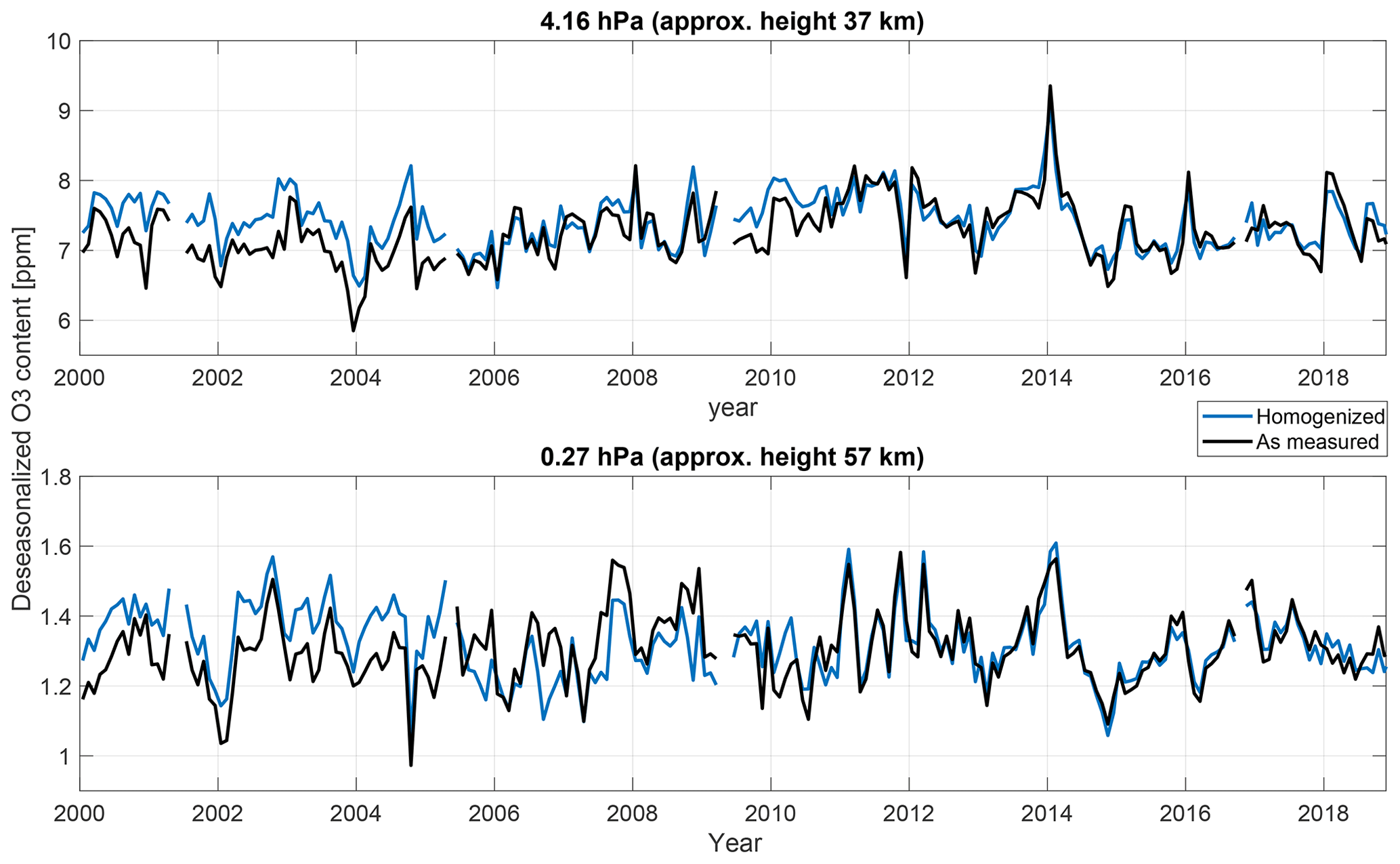
Figure 4 Deseasonalized ozone monthly mean time series before (in black) and after (in blue) the homogenization for a representative layer in the middle stratosphere and in the low mesosphere.

4 Methods

4.1 Diurnal cycle calculation

The amplitude of the ozone diurnal cycle depends on altitude and varies seasonally. Above 0.59 hPa (50 km), the daytime ozone values are 15 %–25 % lower compared to the nighttime values, while at 5 hPa (35 km) afternoon values are up to 3 % larger compared to nighttime values. The ozone diurnal cycle in the mesosphere has been intensively studied (Pallister and Tuck, 1983; Ricaud et al., 1996; Vaughan, 1984). The diurnal cycle of ozone in the stratosphere has been reported in Haefele et al. (2008), and the interannual variations in the ozone diurnal cycle have been described in Studer et al. (2014).

The diurnal ozone cycle is calculated relative to the nighttime value by

$$\begin{array}{}\text{(1)}& {\mathrm{O}}_{\mathrm{3},\mathrm{rel}}={\displaystyle \frac{{\mathrm{O}}_{\mathrm{3}}-{\mathrm{O}}_{\mathrm{3},\mathrm{midnight}}}{{\mathrm{O}}_{\mathrm{3},\mathrm{midnight}}}},\end{array}$$

where O_3,midnight is an average of the ozone values from 22:00 to 02:00 LST at each pressure level.

4.2 Trend calculation

Trend estimates are obtained by fitting a multi-linear regression (MLR) function to the monthly mean ozone time series from each dataset. Trends are calculated for each pressure level independently and form a trend profile. We calculate average daytime (10:00–14:00 LST) and nighttime (22:00–02:00 LST) trends as well as the trends for each hour of the day. The following MLR function is used:

$$\begin{array}{}\text{(2)}& \begin{array}{rl}& {\mathrm{O}}_{\mathrm{3}}\left(t\right)=a+c_{\mathrm{0}}t+\sum _{i=\mathrm{1}}^{\mathrm{2}}{c}_i\sin \left({\displaystyle \frac{\mathrm{2}\mathit{\pi }i}{\mathrm{12}}}t\right)\\ & +\sum _{j=\mathrm{1}}^{\mathrm{2}}{c}_{j+\mathrm{2}}\cos \left({\displaystyle \frac{\mathrm{2}\mathit{\pi }j}{\mathrm{12}}}t\right)+c{}_{\mathrm{5}}\mathrm{SOL}\left(t\right)+c_{\mathrm{6}}{\mathrm{QBO}}_{\mathrm{10}}\left(t\right)\\ & +c_{\mathrm{7}}{\mathrm{QBO}}_{\mathrm{30}}\left(t\right)+c_{\mathrm{8}}\mathrm{ENSO}\left(t\right)+c_{\mathrm{9}}\mathrm{NAO}\left(t\right)+r\left(t\right).\end{array}\end{array}$$

The results are given as a percentage of the respective 2000–2010 mean. The proxies used represent sources of geophysical variability with known influence on stratospheric ozone, including the quasi-biennial oscillation (QBO at 30 and 10 hPa), the 10.7 cm solar radio flux describing the 11-year solar cycle (SOL), the El Niño–Southern Oscillation (ENSO), the North Atlantic Oscillation (NAO) and Fourier components representing the seasonal cycle (annual and semi-annual variations). t is in months, r(t) is the residual, c₀ is the linear component (the trend) and a is the ordinate intercept of the regression line. The data sources for each proxy are provided in the data availability section at the end of this paper.

Stratospheric trends (below 50 km) are derived from data covering 2000 to 2018 while lower-mesospheric trends (above 50 km) are derived from data covering 2010 to 2018. The solar cycle proxy has not been considered in the latter case because of the high probability of correlation with the linear slope when regressing time series shorter than one solar cycle.

All data points are considered with equal weights, and the uncertainty of the fit parameters is estimated from the regression residuals. Residual autocorrelations are removed using the Cochrane–Orcutt transformation (Cochrane and Orcutt, 1949).

5 Results

5.1 Validation

Since the ozone profile time series used in this study is retrieved with an updated version of the OEM Arts/Qpack retrieval (see Sect. 2.1), we carried out a new validation of the Payerne MWR dataset with ground-based and satellite ozone profile measurements.

5.1.1 Profiles of the mean relative differences

Individual Payerne MWR ozone profiles were compared with coincident satellite ozone profiles with a maximal temporal separation of 2 h. The means of the relative differences between each satellite dataset and the Payerne MWR are plotted for the 25–65 km altitude range in Fig. 5a for daytime (10:00–14:00 LST) and Fig. 5b for nighttime (22:00–02:00 LST). The comparison with the HALOE sunset dataset is plotted in the daytime panel and the HALOE sunrise dataset in the nighttime panel, but these should be considered with caution given the low number of coincident measurements. The dotted lines represent the standard errors of the means.

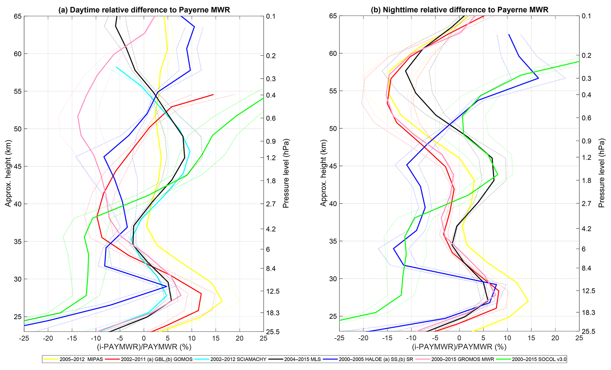
Figure 5 Payerne MWR bias vertical structure: mean of the relative difference between Payerne MWR and satellites MIPAS, MLS, GOMOS, GBL, SCIAMACHY, HALOE (a SS and b SR) and Bern MWR and SOCOL v3.0 CCM, for (a) daytime (10:00–14:00 LST) and (b) nighttime measurements (22:00–02:00 LST).

The spread of the relative differences is as large as ±12 %. Similar differences (i.e., ±5 % to ±10 %) are reported in studies comparing satellite datasets (Laeng et al., 2014; Rahpoe et al., 2015) and comparing ground-based and satellite datasets (Hubert et al., 2016).

The mean relative difference of daytime profiles compared to MLS is approximately between −8 % and +8 % over the 30–65 km altitude range, while the relative difference compared to the HARMOZ datasets is between −10 % and +10 % over the 30–65 km altitude range. A systematic positive bias of the MIPAS, GBL, GOMOS, SCIAMACHY, HALOE and Bern MWR day and night datasets compared with the Payerne MWR is reported below 30 km. The larger relative difference compared to the HARMOZ datasets (when compared to the 5% difference with MLS) can be explained by the choice of the spatial coincidence criteria. The criteria for spatial coincidence (10^∘ by 10^∘) may seem large but is necessary given the smaller number of coincidences. Reducing the spatial coincidence criterion from 10^∘ to 6^∘ in latitude (reducing the box from (41.82^∘ N, 1.95^∘ E, 51.82^∘ N, 11.95^∘ E) to (43.82^∘ N, 1.95^∘ E, 49.82^∘ N, 11.95^∘ E)) reduces the number of matches by more than 50 %. However, the spatial distribution of matches is uneven, with a large number on the north and south borders of the box. This induces a larger bias, given the ozone gradient at these latitudes. The high density of the MLS measurements means that a reduced area can be used for the spatial coincidence criteria without degrading the statistics.

Below 48 km, the nighttime differences compared to MLS, GOMOS and MIPAS are within ±5 %. Above 50 km, the relative differences are as large as −7 % compared to MLS and −15 % compared to MIPAS and GOMOS. The Payerne MWR overestimates nighttime ozone at 55 km compared to all the satellite profiles except HALOE. The positive bias at night at 55 km was reported by Hocke et al. (2007) for a previous version of the Payerne retrieval. Rüfenacht and Kämpfer (2017) show that the emission signal of the secondary ozone layer can alter the nighttime ozone retrieval and thus the ozone values above 0.2 hPa can be overestimated. The a priori profiles and standard deviations used in the Payerne retrieval are identical for day- and nighttime conditions, leading to the effects on the nighttime ozone profiles described in Rüfenacht and Kämpfer (2017), i.e., an overestimation of ozone at 55 km. Considering that the ozone secondary peak intensity is larger at night and that the width of the AVKs of the Payerne MWR dataset is on the order of 17 km in the lower mesosphere, the ozone information in the profile at 55 km is influenced by the ozone content at higher altitudes.

The ±10 % agreement of the Payerne MWR with satellites assesses the quality of the measurements considering the uncertainties of the respective instruments. The systematic 7 % underestimation of ozone at 30 km is under investigation, while the nighttime 15 % overestimation has been assigned to a mesospheric aliasing effect. The agreement between the two Swiss MWRs is described in the next paragraph.

Relative difference compared to the Bern MWR

The mean relative difference between the Bern and Payerne MWRs lies between ±10 % up to 40 km, increasing to a maximum of −10 to −13 % between 47 and 57 km (Fig. 5). Since the measurement setups of the Bern and Payerne MWRs are very similar, we would expect better agreement between the two instruments. However, the Payerne and Bern retrieval procedures differ in the calibration, the a priori climatology used, the uncertainties used for the a priori and measurement covariance matrices, the spectroscopic parameters (pressure broadening), and the temperature profiles used in the forward model. The measurement contribution and total error therefore slightly differ between the two MWRs. Based on a sensitivity study of the retrieval parameters of the Payerne MWR ozone profiles, the influence of the spectroscopic parameters is as high as ±7 % at 50 km, while the influence of the forward model temperature profile is ±2 % at 50 km. Moreover, no period weighting to account for anomalous measurements such as described in Bernet et al. (2019) has been applied to the Bern MWR dataset. Efforts are ongoing to harmonize the retrieval processes and it is future work to harmonize the two data processing chains to determine the sources for the differences.

Relative difference compared to SOCOL v3.0

The Payerne MWR and SOCOL climatological means agree within 15 % at 50 km (Fig. 5). Above this level, the daytime values show differences of similar magnitude, but the nighttime differences are much larger, up to 40 % at 0.2 hPa (60 km). The relative differences also appear to vary with season, with ozone values being closer in NH winter than in summer (not shown). The high time resolution of both the Payerne MWR and SOCOL simulations means that it is possible to derive ozone diurnal cycle profiles (Fig. 6). In the NH midlatitudes, the daytime ozone levels vary with altitude from +4 % at 4 hPa (36 km) to −25 % at 0.2 hPa (60 km) with respect to nighttime values. The comparison of ozone diurnal cycles measured by the Payerne MWR and simulated by SOCOL v3.0 shows good agreement, both with negative values during the day above 0.85 hPa, a minimum at sunrise and a maximum in the afternoon, peaking at 12 hPa and 4 hPa, respectively, for Payerne MWR (Fig. 6a and b). The disagreements in amplitude and in height of transition from the lower-mesospheric to stratospheric diurnal cycle mode are slightly reduced when considering the AVK convolution of SOCOL v3.0 profiles to the Payerne MWR vertical resolution. This is due to the degradation of the model information vertical resolution (Fig. 6c) as described in Studer et al. (2014).

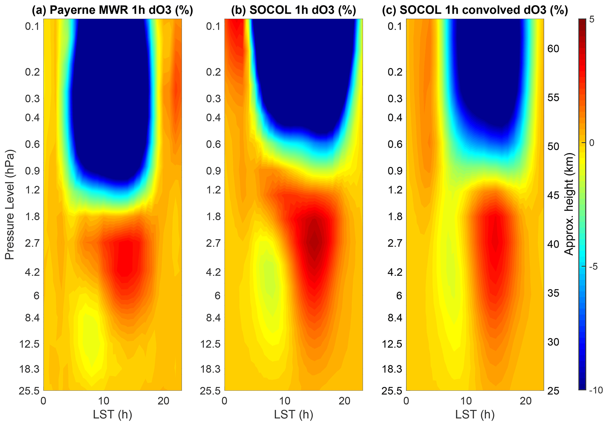
Figure 6 Annual mean O₃ daily cycle measured by (a) Payerne MWR and (b–c) simulated by SOCOL v3.0 with a time step of 1 h.

SOCOL v3.0 overestimates the amplitude of the ozone diurnal cycle in the upper and middle (32–10 hPa) stratosphere and this could be related to the known overestimation of water vapor and upward transport in the model as well as to the positive temperature bias compared to ERA-40 (Stenke et al., 2013).

Despite a modest agreement between the Payerne MWR and SOCOL v3.0 ozone content values, especially above 50 km, the good agreement between the Payerne MWR and SOCOL v3.0 diurnal variations in the 30 to 50 km altitude range makes it possible to consider the comparison of both datasets' variation with LST. Nevertheless, the disagreement in the height of the diurnal cycle extremes has to be considered when comparing trends.

5.2 Multiple linear regression analysis

5.2.1 24 h, daytime, and nighttime trends

Up to 50 km, the 2000–2018 24 h trend estimates are similar at the 95 % confidence level to the 2000–2016 trend profiles of LOTUS NH ground-based datasets (Umkehr, lidar below 40 km) and a range of models as described in Petropavlovskikh et al. (2019) (Fig. 7). At 2 hPa (43 km) the trend is with 2 % per decade significantly positive. We tested the effect of the extended time span on the results. Effects on trends can be noticed below 30 km with a shift towards more positive values, while upper-stratospheric trends do not vary significantly. At 50 km, the 24 h average Payerne MWR trend is 2 % per decade lower than the trends calculated from the Dobson Umkehr, satellite and model datasets used by Petropavlovskikh et al. (2019), which are all positive but nonsignificant at that altitude.

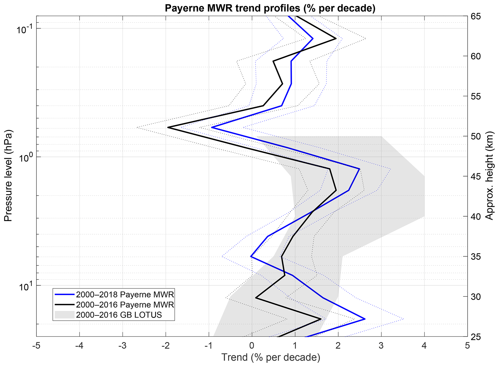
Figure 7 Payerne MWR O₃ trend profiles for the 2000–2016 time range in black and 2000–2018 time range in blue. The dotted lines show the 2σ uncertainties. The shaded area is the full range of LOTUS ground-based 2000–2016 trend profiles.

Day- and nighttime trends for the three MWRs, MLS satellite and SOCOL CCM datasets are plotted in Fig. 8. Panels (c) and (d) show 2000–2016 day- and nighttime trends up to 0.59 hPa (50 km). Panels (a) and (b) show the 2010–2018 day- and nighttime trends in the low mesosphere. The focus here is the comparison of day- and nighttime trend profiles, it being obvious that we cannot directly compare 2000–2016 with 2010–2018 trends. Similarly, the MLO MWR trends cannot be compared to the NH trends.

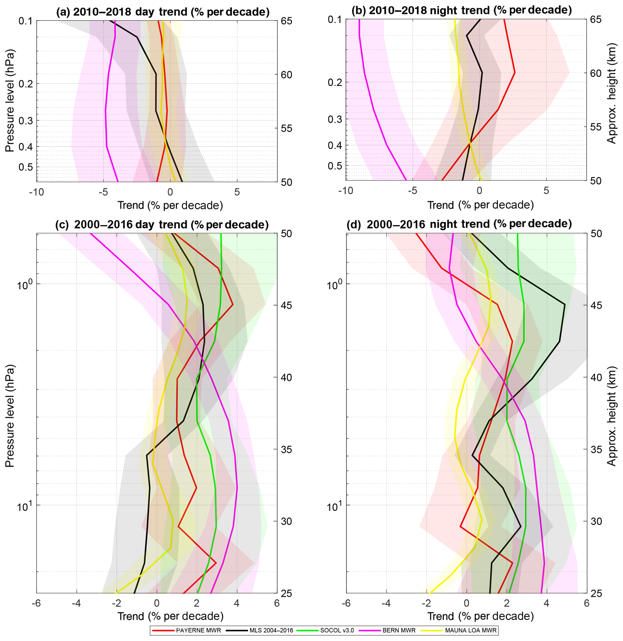
Figure 8 The 2000–2016 stratospheric (c, d) and 2010–2018 low-mesospheric (a, b) day- and nighttime trend profiles for Payerne MWR, MLS, SOCOL v3.0, Bern MWR and 2000–2015 MLO MWR. The shaded areas show the 2σ uncertainties.

Day- and nighttime mid-stratospheric trends do not differ significantly at the 95 % confidence level for the Payerne MWR, SOCOL, MLS satellite or MLO MWR (Fig. 8c, d). The largest, but still not statistically significant, difference between day- and nighttime trends is measured at 45 km, with positive trend estimates ranging from 2 to 4 % per decade for the Payerne MWR and from 2 to 5 % per decade for MLS. The statistically significant difference measured for the Bern MWR at 50 km is probably artificially produced by the 2009 homogenization which does not take into account the measurement contribution variation and/or a variation in the correction offset with LST. A similar behavior was observed for the Payerne MWR before the comprehensive homogenization of the AOS and FFTS datasets.

No significant differences between trends derived from day- and nighttime measuring instruments can therefore be attributed to a systematic measurement schedule difference between the instruments. As below 45 km the diurnal cycle amplitude is minimal at sunrise and maximal in the afternoon, we do not expect any influence of the ozone diurnal cycle on the daytime and nighttime long-term trends at these altitudes. The potential influence of the diurnal cycle (ozone morning minimum and afternoon maximum) at these altitudes will be investigated by considering trends for each hour (see Sect. 5.2.2).

Day- and nighttime lower-mesospheric trends do not differ significantly at 95 % for the Payerne MWR, SOCOL and MLS satellite or for the MLO MWR (Fig. 8a, b). The largest, but still not statistically significant, difference between day- and nighttime trends is measured at 57 km, with trend estimates ranging from 0 to 3 % per decade for the Payerne MWR, and at 62 km, with trend estimates ranging from 0 % to −2 % per decade for MLS. At these altitudes too, no significant differences between trends derived from day- and nighttime measuring instruments can be attributed to a systematic measurement schedule difference, despite the fact that we expected an influence of the ozone diurnal cycle on the trend estimates in this altitude range. The day- and nighttime trends as measured by the Bern MWR are significantly negative in the lower mesosphere. We did not investigate the large negative nighttime trend estimates in this work but, as mentioned in Sect. 5.1.1, intensive efforts are ongoing to homogenize the two Swiss MWRs for the post-2010 period.

5.2.2 Payerne MWR ozone trends as a function of LST

In the stratosphere the ozone diurnal cycle shows a minimum at sunrise (∼12.5 hPa) and a maximum (∼4.16 hPa) in the afternoon (shown in Fig. 6). Long-term trends for each hour of the day were calculated using the method described in Sect. 4.2. This is only possible for the Payerne and Bern MWR datasets and for the SOCOL v3.0 simulations, which all have the necessary hourly time resolution.

Table 1 List of the explanatory variables used in the MLR model.

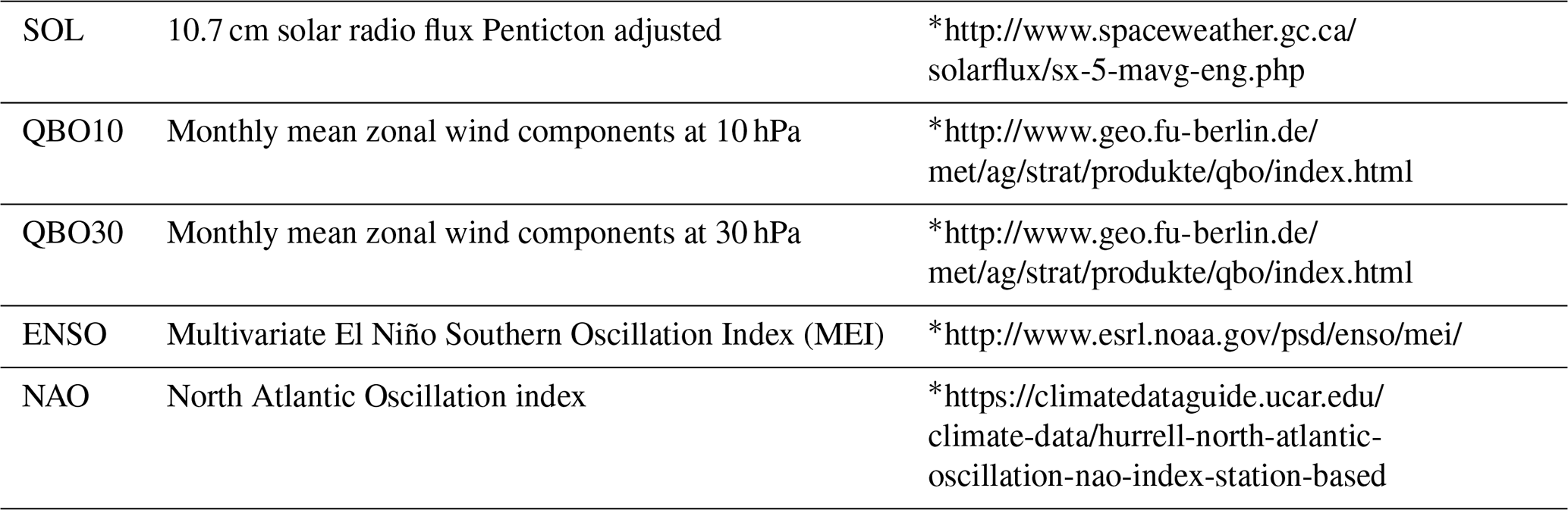
^* Last access: 17 February 2020.

In Fig. 9, one trend estimate in percent per decade is plotted for each pressure level in the stratosphere and each hour of the day without any interpolation. Trend profiles in percent per decade are shown as a function of LST, with hatches indicating values which are not significantly different from zero at the 95 % confidence level. The Payerne MWR mid-stratospheric 2000–2018 trends are represented in Fig. 9a and Bern MWR trends in Fig. 9b. For each pressure level, the variations in ozone trends as a function of LST are small, and the differences are not significant at the 95 % confidence level. The largest, but still not statistically significant, difference is shown between 04:00 and 14:00 h LST at 40 km (Fig. 9c in red). Even when considering the altitude difference between the morning minimum and the afternoon maximum, the long-term ozone trends at the morning minimum (12.5 hPa, 08:00 h LST, in blue) are similar to the long-term ozone trends at the afternoon maximum (4.16 hPa and 14:00 h LST, in black) at the 95 % confidence level.

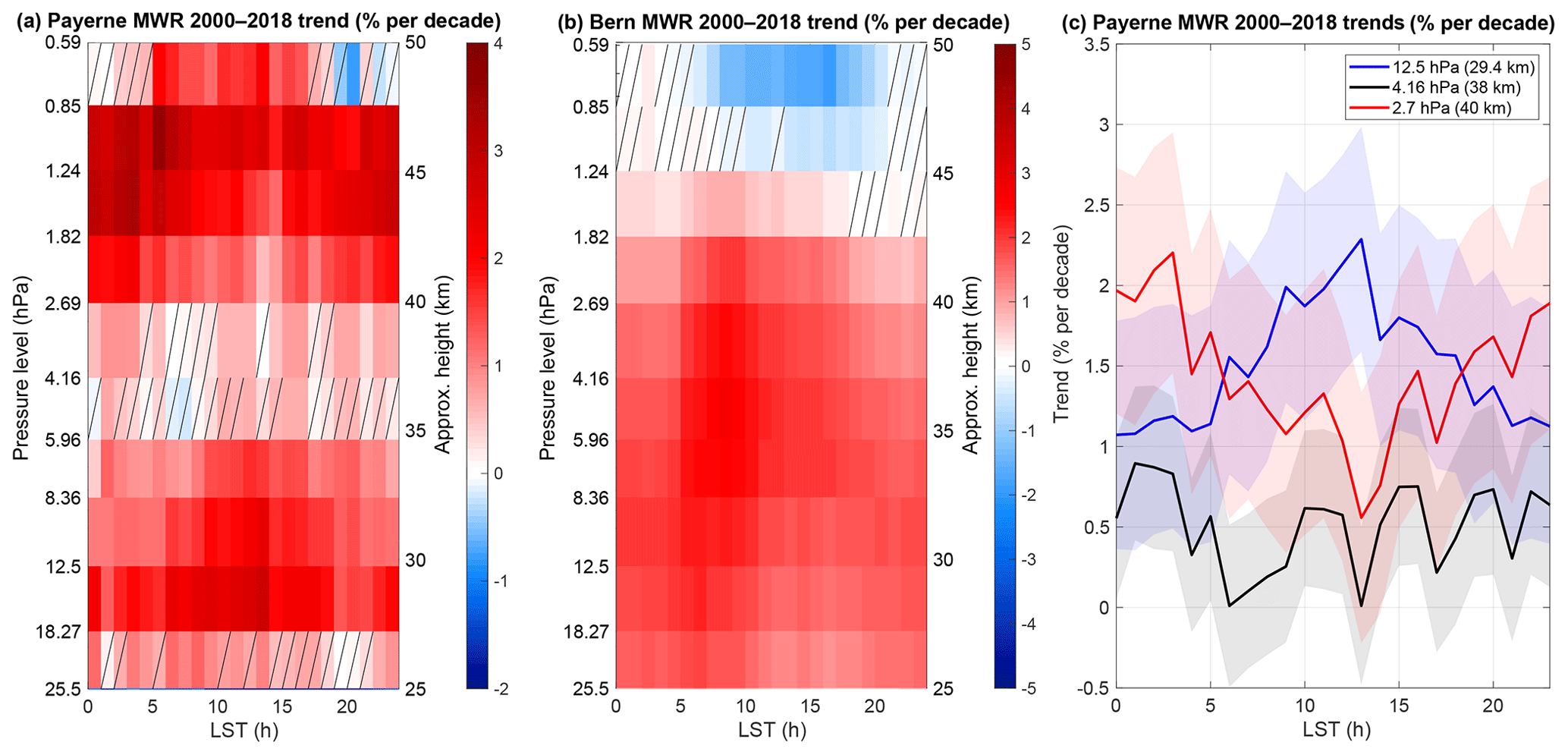
Figure 9 Long-term trends in percent per decade vs. LST for the 2000–2018 period. Trend estimates nonsignificantly different from zero at 95 % are hatched. (a) Payerne MWR 1 h time resolution dataset, (b) Bern MWR 1 h time resolution dataset and (c) Payerne MWR O₃ trends in percent per decade at 2.7 hPa (red), at morning minimum (12.5 hPa, blue) and at afternoon maximum (4.16 hPa, black) pressure levels vs. LST.

5.2.3 SOCOL OH, NO_x and temperature trends as a function of LST

Based on the correlation between long-term stratospheric O₃ and NO_x, active H, and temperature variations and on the similarities of the ozone diurnal variation simulated by SOCOL and measured by the Payerne MWR, we investigate the variation in the NO_x, OH and T trends with LST as an attempt to derive a correlation between ozone trend variation with LST and ozone-influencing-substance trend variations with LST. We derive trends of simulated OH, NO_x and T as a function of LST in the stratosphere. We apply a similar MLR with proxies for the solar cycle, QBO at 30 hPa and 10 hPa, ENSO MEI, and aerosols to monthly mean values for the 2000–2016 period.

Figure 10a shows the SOCOL OH linear trends as a function of LST. SOCOL shows a positive OH trend of 4 % per decade during the day and a nonsignificant trend of −2 % per decade at night. No significant variation in daytime OH trend with LST is seen in the stratosphere. The OH impact on ozone chemistry in this altitude range is very limited when compared to NO_x and Cl (Schanz, 2015). Active H influence increases from 0.3 hPa up but is negligible at pressure levels lower than 2 hPa. During the night, OH disappears rather fast due to the absence of photolysis (OH production) and large OH reactivity (OH loss). The nighttime chemistry is mainly influenced by temperature; thus the nighttime ozone trend simulated by SOCOL should be related to the temperature trends (Fig. 10b) and not to the OH trends.

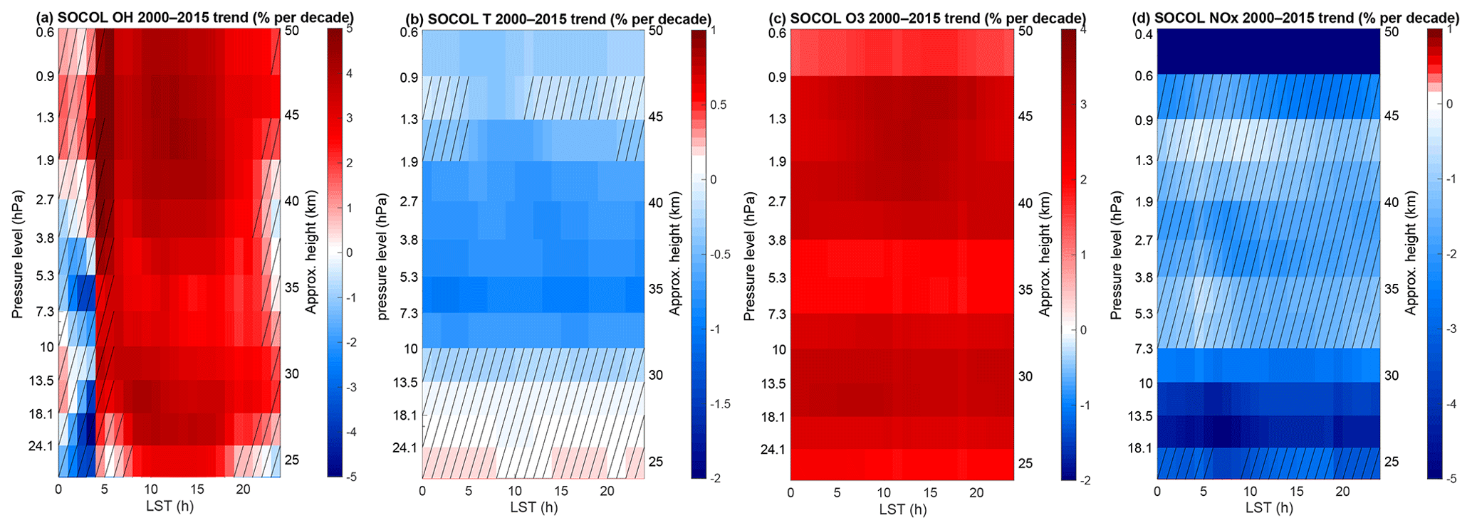
Figure 10 SOCOL v3.0 trends in percent per decade vs. LST (a), OH trends (b), T trends (c), O₃ trends and (d) NO_x trends.

Figure 10b shows the temperature trends as a function of LST. SOCOL shows a slightly negative trend of −1 % per decade for both day- and nighttime between 30 km and 43 km. The negative trends are not significant out of this altitude range. Here again, no significant variation in temperature trend with LST is reported. We can only report a negative correlation between the negative temperature trend and the positive ozone trend independent of LST.

In the stratosphere, NO_x variability plays a key role in ozone changes (Hendrick et al., 2012; Nedoluha et al., 2015a) with a maximum influence at 4 hPa. The same MLR was applied to monthly means of SOCOL-simulated reactive NO_x (${\mathrm{NO}}_x=\mathrm{NO}+{\mathrm{NO}}_{\mathrm{2}}$) for the period 2000–2016. Figure 10d shows the linear trends in simulated NO_x as a function of LST. SOCOL shows a negative trend of −3% per decade in the morning and a statistically nonsignificant negative trend of −1 % per decade in the afternoon. The variation with LST is again not significant at the 95 % confidence level. The simulated NO_x trends agree with those reported by Hendrick et al. (2012), who show negative trends of the NO_x column for 24 h average datasets. Nedoluha et al. (2015b) demonstrated using HALOE (1991–2005) and MLS (2004–2013) measurements that a significant decrease in ozone near 10 hPa in the tropics could be related to a spatially localized but long-term increase in NO_x. They also showed that the response of ozone to NO_x chemistry varies strongly with time of day (Nedoluha et al., 2015a), with ozone destruction through the NO_x cycle increasing from the morning to the afternoon (Schanz, 2015). Here we report negative trends in the morning and in the afternoon, but their difference is not significant at the 95 % confidence level. However, when we consider just the global trends without any distinction by LST, we can see a similar negative correlation between the negative NO_x trend and the positive O₃ trend.

6 Conclusions

The 2000–2018 Payerne MWR dataset has been reprocessed and harmonized to ensure a constant measurement contribution to the ozone profiles and to take into account the effects of the three major technical upgrades (2001, 2005 and 2009). Now the dataset agrees within ±5 % with MLS over the 30 to 65 km altitude range and within ±10 % of the HARMOZ satellite datasets over the 30 to 65 km altitude range. The Payerne MWR agrees within ±15 % up to 50 km with the SOCOL v3.0 CCM. We report a 15 % mean positive offset of the Payerne MWR datasets compared to other datasets at nighttime in the lower mesosphere. The overestimated nighttime ozone of the Payerne MWR is caused by an aliasing of the mesospheric nighttime ozone signal into the lower-mesospheric ozone signal. Post-2000 long-term trends were calculated using MLR applied to the global Payerne MWR dataset and results agree well with other NH ground-based instrument trends published in Petropavlovskikh et al. (2019). Adding 2 more years to the dataset was shown to increase the trends below 30 km. A MLR was also applied to the high-resolution data to assess whether significant trends could be detected in the ozone diurnal cycle. Neither stratospheric nor lower-mesospheric ozone trends vary with LST significantly at the 95 % confidence level. No significant long-term variation in the amplitude of the diurnal cycle is observed even if we consider the altitude difference of the ozone diurnal cycle minimum and maximum. Without any significant variation in the ozone trend with LST, no correlation is possible with the LST variation in temperature, OH and NO_x trends. We can only report a negative correlation between the negative NO_x trend, the negative temperature trend and the positive ozone trend independent of LST in the stratosphere. From our quantification of the ozone trends as a function of LST, we conclude that systematic sampling differences between instruments cannot explain significant differences in trend estimates for the 2000–2018 period in the stratosphere and for the 2010–2018 period in the mesosphere.