Improving the Southern Ocean cloud albedo biases in a general circulation model

The present generation of global climate models is characterised by insufficient reflection of short-wave radiation over the Southern Ocean due to a misrepresentation of clouds. This is a significant concern as it leads to excessive heating of the ocean surface, sea surface temperature biases and subsequent problems with atmospheric dynamics. In this study, we modify cloud microphysics in a recent version of the Met Office's Unified Model and show that choosing a more realistic value for the shape parameter of atmospheric ice crystals, in better agreement with theory and observations, benefits the simulation of short-wave radiation. In the model, for calculating the growth rate of ice crystals through deposition, the default assumption is that all ice particles are spherical in shape. We modify this assumption to effectively allow for oblique shapes or aggregates of ice crystals. Along with modified ice nucleation temperatures, we achieve a reduction in the annual-mean short-wave cloud radiative effect over the Southern Ocean by up to ∼4 W m⁻² and seasonally much larger reductions compared to the control model. By slowing the growth of the ice phase, the model simulates substantially more supercooled liquid cloud.

1 Introduction

One of the major known problems in present-day global climate models is an excess in the absorbed short-wave (SW) radiation over the Southern Ocean (SO) (Trenberth and Fasullo, 2010; Ceppi et al., 2012; Hwang and Frierson, 2013; Williams et al., 2013; Hyder et al., 2018). Chapter 9 of the Fifth Assessment Report of the Intergovernmental Panel on Climate Change (IPCC AR5) (Flato et al., 2014) points out that most of the fifth phase Coupled Model Intercomparison Project (CMIP5) models (Taylor et al., 2012) have a positive SW cloud radiative bias of magnitude of up to 20 W m⁻² over the SO, suggesting that inadequately simulated clouds allow substantially too much sunlight to reach the ocean surface. Several studies have focused on the relation between various aspects of cloud representation in the model and radiation biases pronounced over the SO. Bodas-Salcedo et al. (2012, 2014), using cyclone compositing cluster analyses, suggest the need to increase the optical depth of the low-level clouds and improve the simulation of mid-level cloud regime, to help reduce the biases in the model. By modifying the shallow convection detrainment in their global climate model, Kay et al. (2016) showed that the resultant increase in the supercooled liquid clouds enable large reductions in long-standing climate model SW radiation biases. Furtado et al. (2016) and Lohmann and Neubauer (2018) point towards the significance of mixed-phase clouds and their representation in the models for better representation of SO. In another study by Furtado and Field (2017), the importance of ice microphysics parameterisation in determining the phase composition, and thus the liquid water content of the SO clouds is highlighted.

Discrepancies in the response of clouds to anthropogenic forcings are recognised as a leading reason for a persistent, large spread in the climate sensitivity throughout various generations of climate models (Pachauri et al., 2014). We thus conjecture that this model problem of cloud albedo bias over the SO contributes to this large spread, and thus solving it would increase confidence in projections of anthropogenic climate change (Tan et al., 2016).

In the present study, we investigate the role of parameters involved in atmospheric ice formation within a global climate model in causing the above-mentioned SW radiation bias.

2 Data and experimental setup

We define the SO region as the latitudinal band between 50 and 70^∘ S in this study. The control climate model used in this study is the most recent version of the Met Office's Unified Model, GA7.1 (Walters et al., 2019) with modified microphysics scheme for riming process and several other scientific changes. Appendix A summarises the scientific setup for this model version. The resolution used here is N96L85 (i.e. a horizontal resolution of $\mathrm{1.875}{}^{\circ }\times \mathrm{1.25}{}^{\circ }$ and 85 terrain-following hybrid-height levels extending to 85 km of altitude). It uses the “ENDGAME” dynamical core with a semi-implicit semi-Lagrangian formulation to solve the non-hydrostatic, fully compressible deep-atmosphere equations of motion (Wood et al., 2014)

2.1 Model setup

The control model follows the Atmospheric Model Intercomparison Project (AMIP) climate model development protocol (Gates et al., 1999), using prescribed sea surface temperatures. Excess atmospheric ice has been a persistent concern in the control version of the model, which is especially pronounced over the SO region. Ice clouds have a significant influence on the global climate through their effects on the Earth's radiation budget (e.g. Hartmann and Doelling, 1991; Waliser et al., 2009). Hence, sensitivity setups in our study are aimed at modifications to the microphysics scheme such that the ice growth in the model is controlled. We achieve this by modifying those parameters that control the growth of existing ice by vapour deposition and heterogeneous nucleation of new ice. The classical theory of ice crystal growth uses an electrostatic analogy due to the similarity between the equations governing the water vapour distribution around an ice crystal and the electrostatic potential distribution around an electric conductor of the same shape as the ice crystal (Chiruta and Wang, 2003). Thus, the growth rate of ice crystals by diffusion depends on a shape (also known as capacitance) parameter C, which is a function of both ice crystal size and habit. To determine the ice crystal growth rates in models, it is necessary to know the value of C (Chiruta and Wang, 2003; Hobbs, 1976). The standard equation that is used for calculating the growth rate of ice crystals in the model is

$$\begin{array}{}\text{(1)}& {\displaystyle \frac{\mathrm{d}m}{\mathrm{d}t}}=\mathrm{4}\mathit{\pi }C\left({\mathit{\rho }}_{\mathrm{s}}-{\mathit{\rho }}_{\mathit{\alpha }}\right),\end{array}$$

where C is the capacitance, ρ_α and ρ_s are distributions of vapour densities at and away from the crystal's surface (Houghton, 1950).

From Eq. (1), it is evident that once the value of capacitance C is known, the growth rate of ice crystals can be determined. All other quantities on the right-hand side of Eq. (1) are independent of the shape (Chiruta and Wang, 2003; Hobbs, 1976). Thus, C in the model effectively defines the shape of ice crystals, which in turn is fed to the ice processes of deposition/sublimation and melting without affecting any other ice processes.

Technically the capacitance, C, is defined as 1.0×d in the model where d is the particle maximum size. However, studies have suggested that this value overestimates the evaporation rate of snowflakes by a factor of 2 (Westbrook et al., 2008). It has been shown in other studies based on theory and observations that by changing the value to 0.5×d, models show a significant improvement compared to the traditional approximations used (Westbrook et al., 2008; Field et al., 2008). Thus, in our sensitivity studies, we modified the value to 0.5×d (corresponding to any oblate ellipsoid with two unequal axes, thought to be more appropriate for aggregates and plate-like crystals rather than the assumption of spherical crystals alone). The effect of this change in the shape parameter is tested independently as well as in combination with changing the temperatures at which heterogeneous and homogeneous freezing start in the cloud microphysics scheme. The idea behind modifying the nucleation temperatures is to test the behaviour of capacitance change in a relatively cleaner environment. Basically, the ice nucleation temperature is the temperature at which heterogeneous nucleation of ice first starts to occur in the model. In the control model, this is solely following the temperature dependent function suggested by Fletcher (1962). The default value in the model is −10 ^∘C for heterogeneous nucleation temperature. However, in much cleaner environments, like the SO, ice nucleation might not start at −10 ^∘C as there is a paucity in the ice-nucleating particles (INPs). Hence, in reality, the nucleation temperatures are much colder for these regions. Since we do not have any INP dependency taken into account for ice nucleation temperature in the control model, to test the behaviour of capacitance in such conditions, experiments are conducted by changing the default value of −10 to −40 and −20 ^∘C. The higher threshold of −40 ^∘C has been chosen as it is the maximum temperature at which homogeneous nucleation occurs in the model (i.e. at this temperature, all liquid is instantaneously frozen to form ice particles; Yau and Rogers, 1996). Along with the nucleation temperature in the microphysics scheme, convection scheme also impacts the amount of ice produced in the model through its detrainment temperatures. We thus further modified the convection scheme by changing the detrainment temperatures to be colder than the default values. This thus gives us an overall base to investigate the effect of delaying the heterogeneous ice nucleation in the model. The temperature at which the detraining condensate as ice begins in the model is the start-ice temperature and the temperature at which all condensate is detrained as ice is called the all-ice temperature. Thus, we conducted three sensitivity experiments (henceforth referred to as cap, c_tnuc=-40 and c_tnuc=-20) to be compared against the control model. The values used in our numerical simulations are summarised in Table 1.

Table 1 Values used in the model runs.

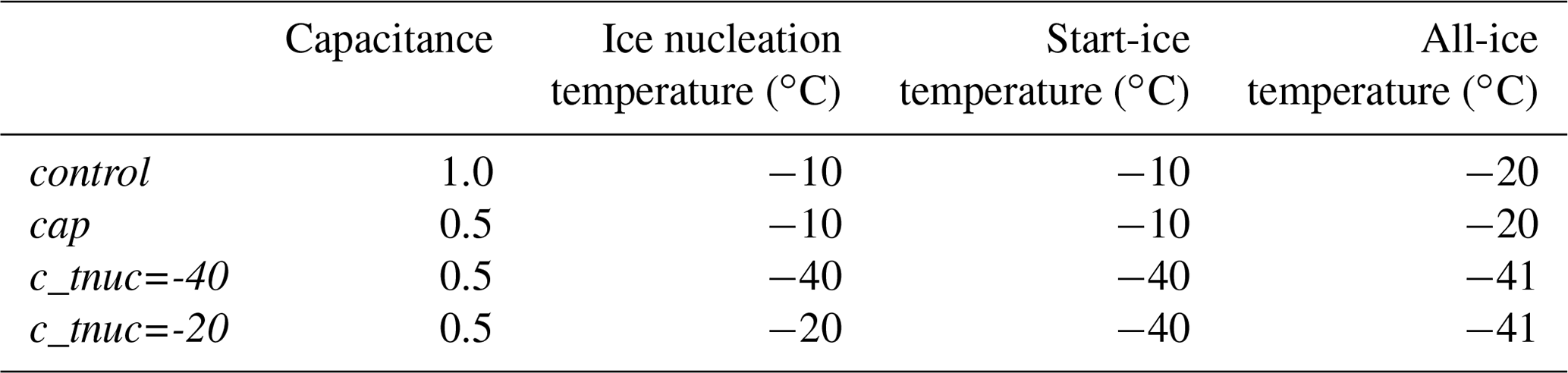
We note that the experiment where nucleation temperature is modified to −40^∘ C (i.e. c_tnuc=-40) is applicable mostly for cleaner environments like the SO but not physically realistic for rest of the world, as mentioned in the previous paragraph. However, it is still a much useful sensitivity scenario to study the importance of detrained ice vs. large-scale freezing. All simulations were run for 22 years under steady-state present-day conditions.

2.2 Observational data

We use the National Aeronautics and Space Administration (NASA) Clouds and the Earth's Radiant Energy System – Energy Balanced And Filled (CERES EBAF Ed4.0, Terra and Aqua) for comparing incoming surface long-wave (LW) and short-wave (SW) as well as the top-of-the-atmosphere (TOA) radiation covering the period 2000 to 2018. This data set, in an earlier version (Loeb et al., 2009) was used in AR5. The overall uncertainty in the monthly all-sky TOA flux for the CERES EBAF Ed4.0 data set is estimated to be 2.5 W m⁻² (for both SW and LW fluxes). For clear-sky TOA, uncertainties in SW and LW fluxes are 5 and 4.5 W m⁻², respectively (Loeb et al., 2018). Direct observations of ocean surface air–sea fluxes are extremely sparse, particularly over the Southern Ocean. There are large uncertainties in the conventional observational surface heat estimates which can affect the evaluation of simulated surface energy budgets. Hence, for the net surface flux comparison, we are using a combination of both TOA fluxes from satellite and ERA-Interim reanalysis energy divergences (assuming atmospheric column energy conservation). This approach considerably constraints the estimates of net surface flux derived from reanalyses. Further details regarding this approach can be found in Hyder et al. (2018).

3 Results

Figure 1 represents the anomaly in the annual and DJF mean distributions of ice water path (IWP) and liquid water path (LWP) for stratocumulus boundary layer clouds in the model in various experiments with respect to the control model, for the Southern Hemisphere (SH). There are seven boundary layer types that have been identified in the model based on the surface stability and capping cloud (Lock et al., 2000). As our focus is mostly on the stratocumulus boundary-layer-type clouds in this study, the cloud types considered in this figure are type 2 indicates boundary layer with stratocumulus over a stable near-surface layer, type 3 indicates well-mixed boundary layer, and type 4 indicates unstable boundary layer with a decoupled stratocumulus (DSC) layer not over cumulus. The IWP and LWP are calculated collectively over these types. The other cloud types in the model are those of stable boundary layer (type 1), boundary layer with decoupled stratocumulus layer over cumulus (type 5), cumulus-capped boundary layer (type 6) and shear-dominated unstable layer (type 7). A similar analysis for the non-stratocumulus cloud types has been provided in the Supplement (Figs. S1 and S2) for annual and DJF means.

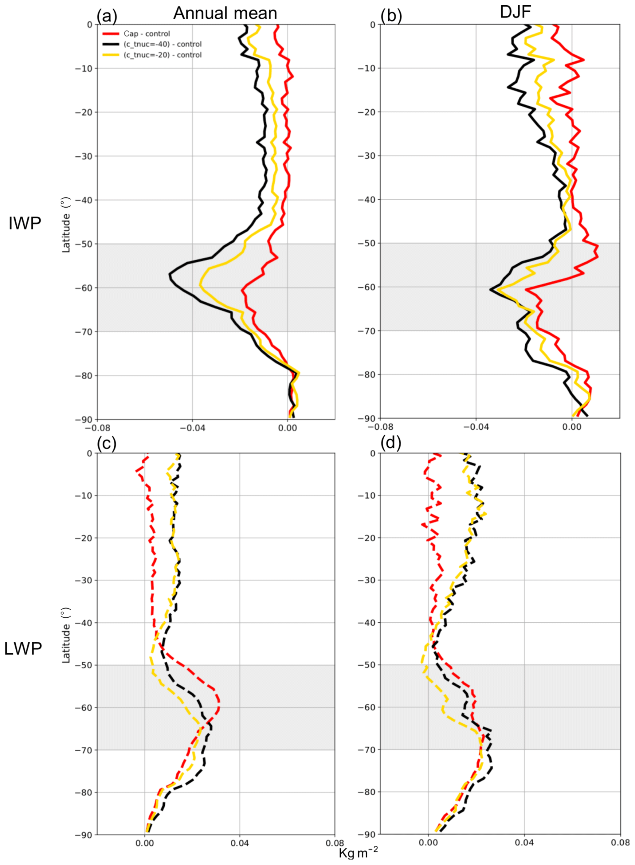
Figure 1 Distribution of zonally averaged anomalies in IWP (solid lines in panels a and b) and LWP (dashed lines in panels c and d) over the stratocumulus boundary-layer-type clouds in the model for the SH. Panels (a) and (c) represent annual mean; (b) and (d) represent DJF mean. The colour codes are as follows: red indicates the anomaly of cap with respect to control, black indicates the anomaly of c_tnuc=-40 with respect to control, and yellow indicates the anomaly of c_tnuc=-20 with respect to control. Values are calculated from 12-hourly instantaneous model output over 22 years. The SO region identified in this study is highlighted in gray.

From Fig. 1a and b, it is evident that there is a noticeable decrease in the IWP in the stratocumulus boundary layer clouds as a result of modified microphysics, which is captured in all sensitivity experiments in both annual and DJF means. The experiment, c_tnuc=-40 (solid black line in Fig. 1a and b) shows the maximum response and the experiment cap (solid red line in Fig. 1a and b) has the minimum decrease in IWP with respect to the control model. Conforming to the decrease in the IWP, there is a corresponding increase in the LWP as well, over the SO region (Fig. 1c and d). However, the response of LWP is more or less similar in all the three experiments with respect to the control model. It is because modification to capacitance value affects both the liquid and ice water contents, while changes to nucleation temperature will have an impact predominantly on IWP. Even any small sensitivity on LWP due to the changes in nucleation temperatures will not have much impact on the zonally averaged stratocumulus types, as the effects are mostly restricted to the shallow boundary types and hence not evident for Fig. 1. Thus, experiments where both capacitance and nucleation temperature are modified will have an added impact on the IWP.

Figure 2 shows the zonal-mean changes in the annual-mean distributions of various radiative fluxes in the model for the SH. Upward fluxes are used for all TOA figures and downward fluxes for surface figures. In all the model experiments, there is a general decrease in the outgoing LW flux at the TOA in the SO region (solid lines in Fig. 2a) with respect to the control model. This is accompanied by a corresponding increase in the outgoing SW flux at the TOA (dotted lines in Fig. 2b), indicating that in all model experiments the planetary albedo has increased versus the control. Except in cap, the decrease in LW radiation at the TOA, in absolute terms, is larger than the increase in SW TOA over the SO. This is visible in the distribution of net radiation at the TOA (i.e. LW plus SW at TOA) (dashed red line in Fig. 2c). For the cap experiment, there is an increase in the net outgoing TOA radiation, whereas for the c_tnuc=-40 and c_tnuc=-20 experiments, it shows a decrease over the SO region.

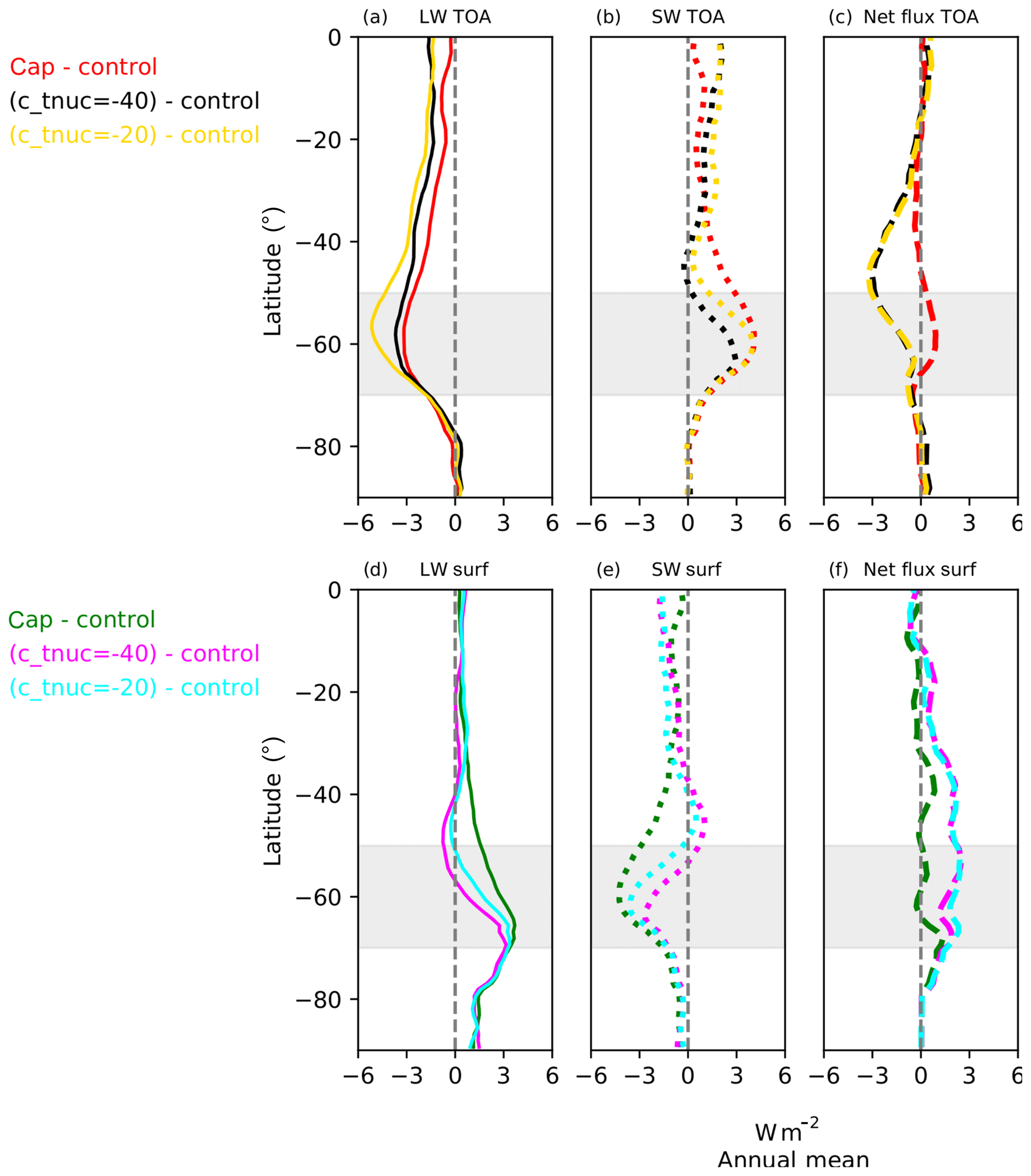
Figure 2 Distribution of zonally averaged annual-mean radiative flux anomalies in various experiments with respect to the control model for the SH. Panels (a–c) represent the TOA (upward) radiative flux anomalies and (d–f) represent the surface (downward) flux anomalies. The solid lines in panel (a) indicate LW at TOA; dotted lines in panel (b) indicate SW at TOA, and dashed lines in panel (c) indicate net flux at TOA (i.e. LW plus SW at TOA). Colour codes for TOA fluxes are as follows: red indicates cap minus control; black indicates (c_tnuc=-40) minus control; and yellow indicates (c_tnuc=-20) minus control. Similarly, the solid lines in panel (d) indicate LW at surface, dotted lines in panel (e) indicate SW at surface, and dashed lines in panel (f) indicate net radiative heat flux at surf (i.e. incoming LW plus SW at surface minus (sensible heat plus latent heat). Colour codes for surface fluxes are as follows: green indicates cap minus control; magenta indicates (c_tnuc=-40) minus control; and cyan indicates (c_tnuc=-20) minus control. Annual-mean values for model are calculated from daily-mean output over 22 years. The SO region identified in this study is highlighted in gray.

The surface distributions of the radiative fluxes are represented in Fig. 2d to f. In all the experiments, the net downward LW radiation at the surface shows an increase over the SO (solid lines in Fig. 2d) with respect to the control model. The corresponding SW component shows a decrease over SO (dotted lines in Fig. 2e). The distribution of anomaly in the radiative heat fluxes with respect to the control model is represented by dashed lines in Fig. 2f. It primarily represents the difference between total net downward surface radiation and total heat flux at the surface, i.e. (incoming LW plus SW at surface) minus (sensible heat flux plus latent heat flux). Although there is an improvement (i.e. reduction) in the downward SW component (dotted lines in Fig. 2e), due to the compensating increase in the LW component (solid lines in Fig. 2d), there is a net increase in the heat flux into the surface over the SO (dashed lines in Fig. 2f) in almost all experiments. However, the net radiative heat flux shows a tendency of slight decrease over SO for the cap experiment with respect to the control model (dashed green line in Fig. 2f).

Figure 3 shows the distributions of various radiative fluxes in the model for the SH for the DJF season. The radiative fluxes show a more pronounced response during the austral summer season. The net radiative flux at TOA (dashed lines in Fig. 3c) shows an increase over the SO for all the experiments unlike the annual-mean distribution where only the cap experiment shows an increase. Similarly, the net radiative heat flux at the surface (dashed lines in Fig. 3f) shows a general decrease over the SO in all the experiments with respect to the control model for the DJF season, whereas in annual mean, only the cap experiment showed a decrease in net surface flux.

Figure 3 Similar to Fig. 2 but for the DJF season.

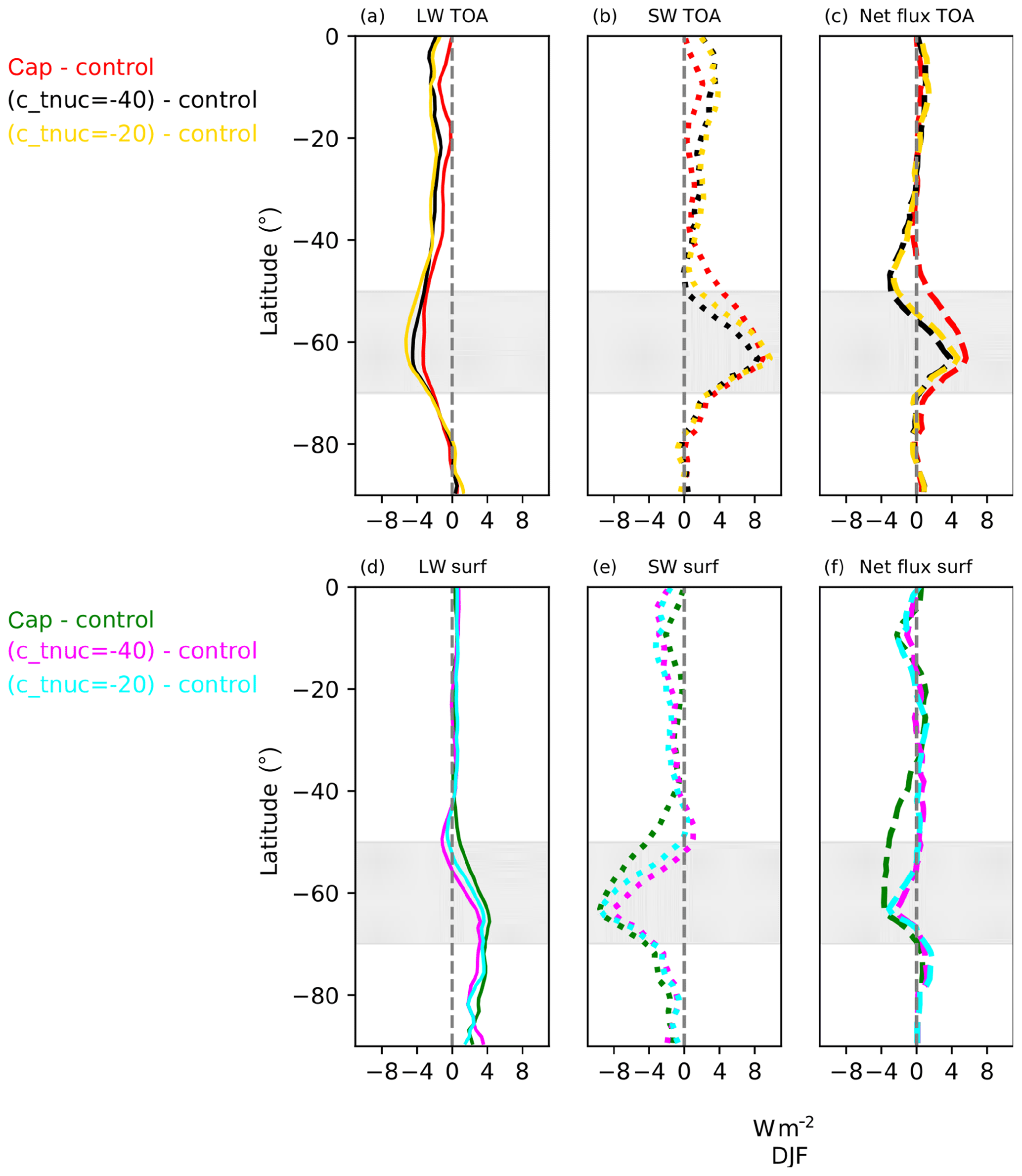
Figure 4 represents the difference between the model experiments and observational data for annual mean. It is mainly intended to provide a reference for the model behaviour in terms of radiative fluxes. By comparing Figs. 2 and 4, it can be seen that it is the LW component that shows similar signs of response (solid lines in Figs. 2a, d and 4a, d) compared to SW for SO region. But the net fluxes show mostly similar signs of response in both TOA (Figs. 2c and 4c) and surface (Figs. 2f and 4f) except for the net TOA flux in the cap experiment (dashed red line in Fig. 2c).

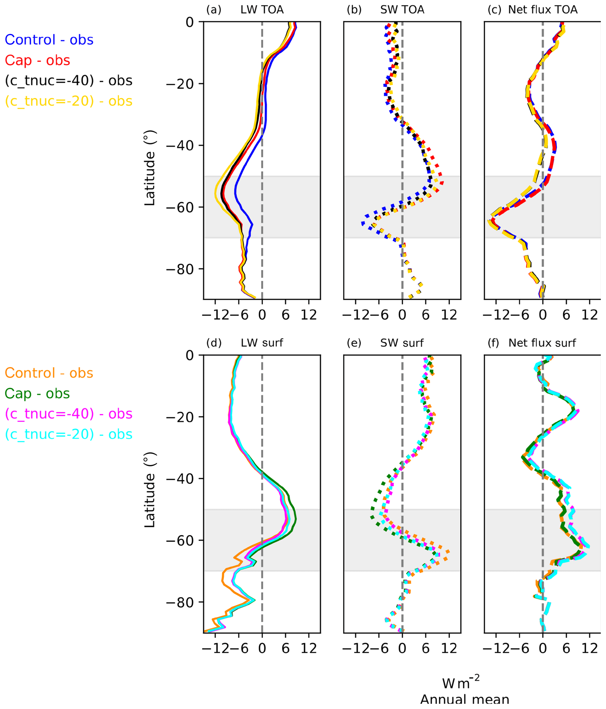
Figure 4 Distribution of zonally averaged annual-mean radiative flux anomalies in various model experiments with respect to observations for the SH. Panels (a–c) represent the TOA (upward) radiative flux anomalies and (d–f) represent the surface (downward) flux anomalies. The solid lines in panel (a) indicate LW at TOA, dotted lines in panel (b) indicate SW at TOA, and dashed lines in panel (c) indicate net flux at TOA (i.e. LW plus SW at TOA). Colour codes for TOA fluxes are as follows: blue indicates control minus obs; red indicates cap minus obs; black indicates (c_tnuc=-40) minus obs; and yellow indicates (c_tnuc=-20) minus obs. Similarly, the solid lines in panel (d) indicate LW at surface, dotted lines in panel (e) indicate SW at surface, and dashed lines in panel (f) indicate net radiative heat flux at surface (i.e. incoming LW plus SW at surface minus (sensible heat plus latent heat). Colour codes for surface fluxes are as follows: orange indicates control minus obs; green indicates cap minus obs; magenta indicates (c_tnuc=-40) minus obs; and cyan indicates (c_tnuc=-20) minus obs. Annual-mean values for model are calculated from daily-mean output over 22 years. The net surface flux observational data are a combination of both TOA fluxes from satellite and ERA-Interim reanalysis energy divergences (details in Sect. 2.2). The SO region identified in this study is highlighted in gray.

Figure 5 shows the zonally averaged annual and DJF mean distributions of the anomaly in the SW cloud radiative effect (SW CRE) between different model experiments with respect to the control model. The SW CRE shows the impact of cloud on TOA SW flux and is calculated by taking the anomaly of TOA SW flux between the clear-sky and all-sky conditions. The reduction in the SW radiative flux over SO is more pronounced in the DJF season (Fig. 5b) with the c_tnuc=-40 experiment showing the minimum reduction in SW CRE compared to the control model.

Figure 5 Distribution of zonally averaged SW CRE anomalies over the SH in various experiments with respect to the control model for (a) annual mean and (b) DJF mean. The colour codes are as follows: red indicates cap minus control, black indicates (c_tnuc=-40) minus control; and yellow indicates (c_tnuc=-20) minus control. Values are calculated from daily-mean output over 22 years. The SO region identified in this study is highlighted in gray.

Figure 6 shows the annual and DJF mean spatial distributions of the anomaly in SW CRE between different model experiments with respect to the control model. It is evident from Fig. 6 that there is a general improvement (i.e. a reduction) in the SW CRE over the SO region in all three experiments compared to the control model. The reduction is more pronounced in the cap experiment (Fig. 6a and d). The response in c_tnuc=-40 is the minimum (Fig. 6b and e). As expected, the response is more robust for the DJF season in all experiments with respect to the control model (Fig. 6d to f).

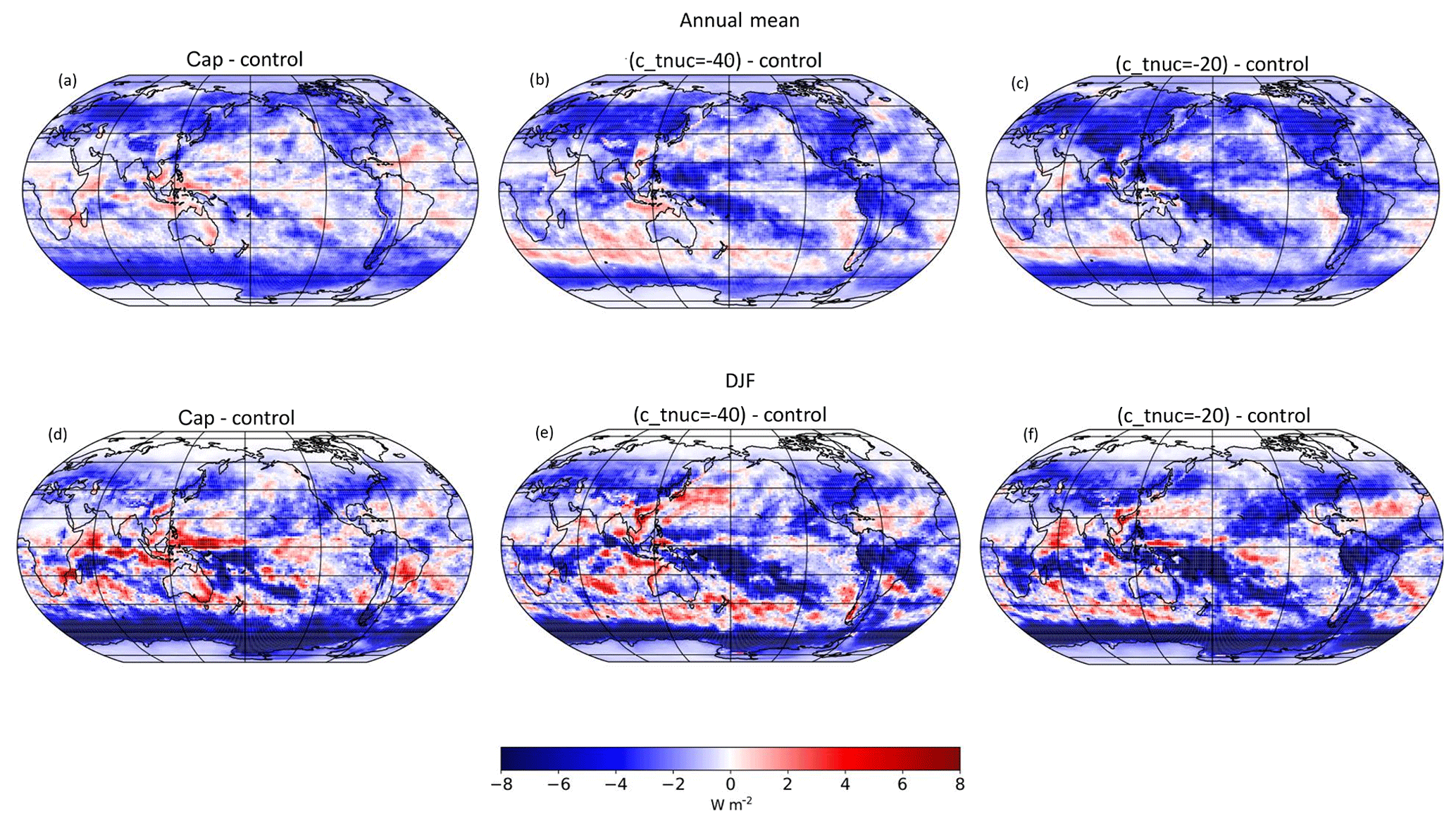
Figure 6 Spatial distributions of annual-mean (a–c) and DJF mean (d–f) SW CRE anomaly at TOA in different experiments with respect to the control model. (a, d) cap minus control, (b, e) (c_tnuc=-40) minus control, (c, f) (c_tnuc=-20) minus control. Values are calculated from daily-mean output over 22 years.

Figure 7 shows the spatial distribution of TOA SW CRE anomaly between various model simulations with respect to the CERES TOA data. As evident from Fig. 7a, the control model does have an excess in the absorbed SW radiation over the SH high latitudes like many other global models. Comparing Fig. 7a with b–d, it can be seen that the changes in microphysics parameterisation have improved the SW biases over the SO. In general, there is an increase in the reflected SW radiation over the SO compared to the control model. The values for annual-mean SW CRE biases in the model experiments (in comparison to both the control model as well as observational data) have been summarised in Table S1 of the Supplement.

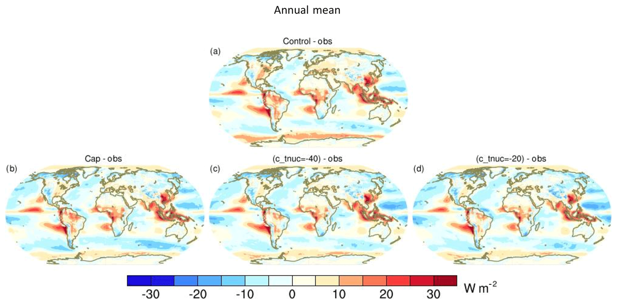
Figure 7 Spatial distributions of annual-mean SW CRE anomaly at TOA in different model simulations with respect to the CERES TOA data. Panel (a) indicates control minus obs; (b) cap minus obs, (c) (c_tnuc=-40) minus obs; (d) (c_tnuc=-20) minus obs. Model data are calculated from daily-mean output over 22 years. Observational (CERES EBAF TOA) data consist of monthly-mean values covering the period 2000–2018.

It is to be noted that the tropical regions do not show much reduction in the SW CRE in response to the capacitance changes. While the SO does show significant reduction in SW CRE with respect to the control model, especially for the cap experiment (Fig. 6a and d), the tropical regions still show an increase. In an earlier study by Furtado et al. (2016), using a similar version of the control model (numerical weather prediction (NWP) configuration), it has been shown that for tropics and subtropics there is a general tendency by the model to overpredict the LWP in response to microphysics modifications. Increasing the stratiform cloud LWP will cause more SW radiation to be reflected back to space. But over the SO, this effect is beneficial because the control model already has a large negative bias in outgoing SW radiation in that region. Basically, in tropics or quasi-steady-state features like that of the fronts, the capacitance does not have much of an impact compared to more dynamic sites like that of supercooled liquid clouds (Furtado et al., 2016, 2015).

Generally, the impact of ice nucleation temperature experiments (c_tnuc=-40 and c_tnuc=-20) on fluxes is more mixed than using capacitance change alone (cap). The detrimental effects due to changes in the ice nucleation temperature could be mostly attributed to the changes in the vertical distribution of clouds affecting not just the low clouds but also the high clouds. By changing the nucleation temperature, essentially the level at which freezing occurs is modified. When the freezing of water in lower levels is delayed, it results in cirrus clouds at higher atmospheric levels. This can change the high cloud characteristics thus affecting both LW and SW.

4 Discussion

Errors in the representation of ice clouds is one of the major shortcomings in many of the present-day global climate models and this can have a significant influence on the global climate through their effects on the Earth's radiation budget (Hartmann and Doelling, 1991; Waliser et al., 2009). These errors are mostly coupled to an underestimation of supercooled liquid clouds and are of particular importance in the SO regions that are characterised by abundant supercooled liquid clouds (Kay et al., 2016; Bodas-Salcedo et al., 2016; Huang et al., 2012; Hu et al., 2010). When ice and supercooled liquid coexist, the ice grows at the expense of the liquid by the Wegener–Bergeron–Findeisen (WBF) mechanism (Wegener, 1911; Bergeron, 1935; Findeisen, 1938). Acknowledging the complexities in representing the many possible background microphysical processes that are responsible for this in a global climate model, the primary idea of modifying the shape parameter of ice crystals is to reduce the rate of depositional growth of ice particles. This reduction essentially slows down the deposition growth of ice crystals, which leaves more water vapour to be available for condensation into liquid phase particles. By lowering the value of capacitance to 0.5×d, we model a decrease in the IWP and an associated increase in the LWP over the SO region (Fig. 1). As a result of this increase in LWP, the outgoing SW fluxes are increased (dotted lines in Figs. 2b and 3b), i.e. an increased LWP corresponds to brighter clouds reflecting more sunlight. This results in a decrease of the downwelling short-wave radiation reaching the surface.

Our choice of 0.5×d for capacitance is based on theory and observational studies (Field et al., 2008; Westbrook et al., 2008). The control model has improved in terms of SO cloud albedo bias with this value than with the default value of 1.0×d. However, as seen in Fig.7, even though the SO has shown signs of improvement, biases still remain especially in the tropics. As already mentioned before, previous studies using a similar NWP configuration of the control model have suggested that the value of depositional capacitance is important mostly for non-equilibrium situations like mixed phase, whereas for quasi-steady frontal states and tropics, capacitance might not be very significant (Furtado et al., 2016, 2015). Therefore, even if the same value for capacitance could be applied globally, the only regions where it will make noticeable differences are those of the mixed-phase cloud regions (like SO).

Earlier studies have also suggested that some cloud microphysics parameterisations produce unrealistically bright clouds, especially over the Northern Hemisphere (NH) (Furtado et al., 2016). In our control model, the SW biases over the NH were smaller than those over the SO and further brightening of modelled NH clouds is undesirable (Furtado et al., 2016). While the changes to nucleation temperature have a significant impact on the tropics as well, the capacitance changes are more localised to the high latitudes.

Our study shows that while modifying the capacitance is clearly benefiting the SO region SW radiative fluxes, there is some compensating effect from the LW TOA fluxes. As already discussed, the SW anomaly is thought to be mostly due to a lack of liquid clouds in the atmosphere. By targeting the capacitance, the loss of liquid in mixed-phase conditions is reduced, which results in an improvement in the outgoing SW TOA. However, this improvement in SW TOA always leads to an increase in the LW component due to thick clouds, which is unfortunately unavoidable. The annual-mean biases in TOA radiative fluxes along with RMSE values in comparison with observational data have been provided in Tables S2 and S3 of the Supplement. The SO RMSE values for SW TOA tend to be lower than global values as expected. Although the bias in SW TOA over SO has improved in general compared to the observational data, that improvement does not reflect much in the RMSE values. While an in-depth analysis of compensating errors from LW TOA is beyond the scope of this particular study, it is a significant aspect and provides an interesting outlook for future studies.

Also, several recent studies point towards the significance of INP for cloud phase (Kanji et al., 2017; Vergara-Temprado et al., 2018). A further development of the research outlined here could be to make glaciation explicitly dependent on INP concentration to attend to the persisting model biases in other regions of the world as well. At present, in most global climate models, cloud phase is determined only by a threshold temperature like in our control model. Vergara-Temprado et al. (2018), by combining a high-resolution NWP model with estimates of INP concentration over the SO, simulated clouds that are far more reflective than those in current global climate models, in better agreement with satellite observations.

5 Conclusions

In this study, we reduce the annual-mean SW radiation biases over SO in a recent version of the UK Met Office's Unified Model by up to ∼4 W m⁻² and seasonally up to ∼8 W m⁻² compared to the control model. This and other contemporary climate models are characterised by excess cloud ice causing biases in SW radiation which are especially pronounced over the SO. Here, we modify the capacitance or shape parameter which represents ice crystal shape and habit. In our sensitivity studies, we reduce this parameter from 1.0×d to 0.5×d (corresponding to any oblate sphere shape in general, where the horizontal axes are longer than the vertical axis and more representative of an aggregate or flat ice crystal) and thus delaying the depositional growth of ice particles. This leads to an increase in liquid water in stratiform clouds and consequently increases the outgoing SW over the SO. We also examine the impact of changing other temperature thresholds in the cloud microphysics scheme for the onset of heterogeneous ice production. Our analysis shows that the SW radiation bias has significantly reduced over the SO after the modification of these parameters. However, disparities still exist in other regions. INPs that are currently not represented in the cloud microphysics scheme might be a factor in this model behaviour. The fact that nucleation temperature changes currently is associated with the same effects globally is undesirable, it further motivates the future work to couple the nucleation temperature to a prognostic or the least a regionally specified INP concentration.

Appendix A

Several changes were introduced in the control model used in this study relative to its predecessor (GA7.1) (Walters et al., 2019; Brown et al., 2012). These changes range from minor bug fixes and optimisation techniques to major science changes in the convection, large-scale precipitation, boundary layer and radiation schemes. As far as our study is concerned, the main modification to GA7.1 is the inclusion of the modified microphysics scheme which includes a shape dependence of riming rates using the parameterisation by Heymsfield and Miloshevich (2003), as a measure to prevent small liquid droplets from riming (Furtado and Field, 2017).

Some of the modifications in the convection scheme include that of a prognostic-based convective entrainment rate, implementation of a new melting scheme to remove larger spikes in convective heating in the mid-troposphere, a revised forced detrainment calculation and a corrected evaporation of convective precipitation to remove existing errors.

The modified boundary layer scheme also includes changes to reduce vertical resolution sensitivity and an improved turbulent kinetic energy diagnostic and how it is used for aerosol activation. The change in the radiation scheme is the implementation of spectral dispersion suggested by Liu et al. (2008) to improve the simulation of the first aerosol indirect effect.

A brief overview of the science changes is available in the Unified Model Newsletter December 2017 edition (Research and Model Development News, pages 1–12. This document is included along with the model data at https://doi.org/10.5281/zenodo.3775170; Varma, 2019).