The increasing atmospheric burden of the greenhouse gas sulfur hexafluoride (SF₆)

We report a 40-year history of SF₆ atmospheric mole fractions measured at the Advanced Global Atmospheric Gases Experiment (AGAGE) monitoring sites, combined with archived air samples, to determine emission estimates from 1978 to 2018. Previously we reported a global emission rate of 7.3±0.6 Gg yr⁻¹ in 2008 and over the past decade emissions have continued to increase by about 24 % to 9.04±0.35 Gg yr⁻¹ in 2018. We show that changing patterns in SF₆ consumption from developed (Kyoto Protocol Annex-1) to developing countries (non-Annex-1) and the rapid global expansion of the electric power industry, mainly in Asia, have increased the demand for SF₆-insulated switchgear, circuit breakers, and transformers. The large bank of SF₆ sequestered in this electrical equipment provides a substantial source of emissions from maintenance, replacement, and continuous leakage. Other emissive sources of SF₆ occur from the magnesium, aluminium, and electronics industries as well as more minor industrial applications. More recently, reported emissions, including those from electrical equipment and metal industries, primarily in the Annex-1 countries, have declined steadily through substitution of alternative blanketing gases and technological improvements in less emissive equipment and more efficient industrial practices. Nevertheless, there are still demands for SF₆ in Annex-1 countries due to economic growth, as well as continuing emissions from older equipment and additional emissions from newly installed SF₆-insulated electrical equipment, although at low emission rates. In addition, in the non-Annex-1 countries, SF₆ emissions have increased due to an expansion in the growth of the electrical power, metal, and electronics industries to support their continuing development.

There is an annual difference of 2.5–5 Gg yr⁻¹ (1990–2018) between our modelled top-down emissions and the UNFCCC-reported bottom-up emissions (United Nations Framework Convention on Climate Change), which we attempt to reconcile through analysis of the potential contribution of emissions from the various industrial applications which use SF₆. We also investigate regional emissions in East Asia (China, S. Korea) and western Europe and their respective contributions to the global atmospheric SF₆ inventory. On an average annual basis, our estimated emissions from the whole of China are approximately 10 times greater than emissions from western Europe. In 2018, our modelled Chinese and western European emissions accounted for ∼36 % and 3.1 %, respectively, of our global SF₆ emissions estimate.

1 Introduction

Of all the greenhouse gases regulated under the Kyoto Protocol (United Nations, 1998), SF₆ is the most potent, with a global warming potential (GWP) of 23 500 over a 100-year time horizon (Myhre et al., 2013). In practical terms, this high GWP means that 1 t of SF₆ released to the atmosphere is equivalent to the release of 23 500 t of carbon dioxide (CO₂). However, the low atmospheric mixing ratio of SF₆ relative to CO₂ limits its current contribution to total anthropogenic radiative forcing to about 0.2 % (Engel et al., 2019). Nevertheless, with a long atmospheric residence time of 3200 years, almost all the SF₆ released so far will have accumulated in the atmosphere and will continue to do so (Ravishankara et al., 1993).

Vertical profiles of SF₆ mixing ratios, collected from balloon flights up to an altitude of about 37 km, indicated that there is very little loss of SF₆ due to photochemistry in the troposphere and lower stratosphere (Harnish et al., 1996; Patra et al., 1997). Using an improved atmospheric chemical transport model, Patra et al. (2018) reported significantly older age of air (AoA) in the stratosphere, and Krol et al. (2018), based on a comparison of six global transport models, showed that upper stratospheric AoA varied from 4 to 7 years among the models. It has been suggested that SF₆ may have a shorter atmospheric lifetime of 1937±432 years (Patra et al., 1997), 580–1400 years (Ray et al., 2017), or 1120–1475 years (Kovács et al., 2017). However, these shorter, but still very long, SF₆ lifetimes would not significantly affect SF₆ emissions estimated from atmospheric trends (Engel et al., 2019). Given the very long lifetime of SF₆, compared to the period of our study, uncertainties in this term had a small influence on the outcome. For example, changing the lifetime from 3000 to 1000 years changed the derived emissions by around 1 %, which is smaller than the derived uncertainties.

Since the 1970s, SF₆ has been used mainly in high-voltage electrical equipment as a dielectric and insulator in gas-insulated switchgear, gas circuit breakers, high-voltage lines, and transformers. Sales compiled from 1996–2003 by producers in Europe, Japan, USA, and South Africa (not including China and Russia) showed that, on an annual average basis, 80 % of the SF₆ produced during this period was consumed by electric utilities and equipment manufacturers for electric power systems (EPA, 2018). Percentage sales, averaged from 1996 to 2003, for other end-use applications included the magnesium industry (4 %), electronics industry (8 %), and uses relating to the adiabatic properties of SF₆ (3 %), e.g. incorporating SF₆ into tyres, tennis balls, and the soles of trainers as a gas cushioning filler (Palmer, 1996). For example, in 1997 Nike used 277 t (∼0.25 Gg) of SF₆ as a filler in its shoes (Harnish and Schwarz, 2003). Other uses in particle accelerators, optical fibre production, lighting, biotechnology, medical, refining, pharmaceutical, laboratory, university research, and sound-proof windows accounted for around 5 % of sales (Smythe, 2004).

Emissions from electrical equipment can occur during production, routine maintenance, refill, leakage, and disposal (Niemeyer and Chu, 1992; Ko et al., 1993). Random failure or deliberate or accidental venting of equipment may also cause unexpected and rapid high levels of emissions. For example, a ruptured seal caused the release of 113 kg of SF₆ in a single event in 2013 (Scottish Hydro Electric, 2013). We assume that such random events are generally not recorded when tabulating bottom-up emission estimates, which would lead to an underestimate in the reported inventories.

Historically, significant emissions of SF₆ occurred in magnesium smelting, where it was used as a blanketing gas to prevent oxidation of molten magnesium; in the aluminium industry, also as a blanketing gas; and in semiconductor manufacturing (Maiss and Brenninkmeijer, 1998). These industries and the electrical power industry accounted for the majority of SF₆ usage in the USA (Ottinger et al., 2015). A report on limiting SF₆ emissions in the European Union also provided estimates of emissions from sound-proof windows (60 Mg) and car tyres (125 Mg) in 1998, although these applications appear to have been largely discontinued due to environmental concern (Schwarz, 2000).

Sulfur hexafluoride has also been used as a tracer in atmospheric transport and dispersion studies (Collins et al., 1965; Saltzman et al., 1966; Turk et al., 1968; Simmonds et al., 1972; Drivas et al., 1972; Drivas and Shair, 1974). The combined SF₆ emissions from reported tracer studies (Martin et al., 2011) were approximately 0.002 Gg. Unfortunately, the amounts of tracer released are often not reported, and we conservatively assume that these also amounted to ∼0.002 Gg, providing a total estimate of about 0.004 Gg (4 t) released from historical SF₆ tracer studies. Emissions from natural sources are very small (Busenberg and Plummer, 2000; Vollmer and Weiss, 2002; Deeds et al., 2008).

The earliest measurements of SF₆ in the 1970s reported a mole fraction of <1 pmol mol⁻¹ (or ppt, parts per trillion) (Lovelock, 1971; Krey et al., 1977; Singh et al., 1977, 1979). Intermittent campaign-based measurements during the 1970s and 1980s reported an increasing trend. However, it was not until the 1990s that a near-linear increase in the atmospheric burden, throughout the 1980s, was reported (Maiss and Levin, 1994; Maiss et al., 1996, Geller et al., 1997). Fraser et al. (2004) described gas chromatography with electron capture detection (GC-ECD) measurements of SF₆ at Cape Grim, Tasmania, and noted a long-term trend of 0.1 pmol mol⁻¹ yr⁻¹ in the late 1970s increasing to 0.24 pmol mol⁻¹ yr⁻¹ in the mid-1990s. However, after 1995 the annual average growth rate from 1996 to 2000 declined by 12.5 % to 0.21 pmol mol⁻¹ yr⁻¹, coincident with a ∼32 % decrease in annual sales and prompt releases of SF₆ over this same time period (as noted in Table S2 of the RAND report).

Subsequent reports noted a continuing growth in global mole fractions, with an average growth rate of 0.29±0.02 pmol mol⁻¹ yr ⁻¹ after 2000 (Rigby et al., 2010), reaching 6.7 pmol mol⁻¹ at the end of 2008 (Levin et al., 2010). This increase in the atmospheric burden of SF₆ was also reported by Elkins and Dutton (2009). Measurement of SF₆ in the lower stratosphere and upper troposphere was reported to be 3.2±0.5 pmol mol⁻¹ at 200 mbar in 1992 (Rinsland et al., 1993). These atmospheric observations have been used to infer global emission rates (top-down estimates). Geller at al. (1997) derived a global emission rate of 5.9±0.2 Gg yr⁻¹ in 1996, which by 2008 had increased to 7.2±0.4 Gg yr⁻¹ (Levin et al., 2010) or 7.3±0.6 Gg yr⁻¹ (Rigby et al., 2010) and to 8.7±0.4 Gg yr⁻¹ by 2016 (Engel et al., 2019).

Regional inverse modelling studies indicated that emissions have increased substantially from non-Annex-1 parties to the UNFCCC, particularly in eastern Asia, and that these increases have offset the reduction in emissions from Annex-1 countries (Rigby et al., 2011, 2014; Fang et al., 2014). Rigby et al. (2010) showed an increasing trend in emissions from Asian countries growing from 2.7±0.3 Gg yr⁻¹ in 2004–2005 to 4.1±0.3 Gg yr⁻¹ in 2008. This rise was large enough to account for all the global emissions growth between these two periods. Similarly, Fang et al. (2014) found that eastern Asian emissions accounted for between 38±5 % and 49±7 % of the global total between 2006 and 2012, with China the major contributor of emissions from this region. Consistent regional estimates, within the uncertainties, were also reported for China: 0.8 (0.53–1.1) Gg yr⁻¹ from October 2006 to March 2008 (Vollmer et al., 2009); 1.3 (0.23–1.7) Gg yr⁻¹ in 2008 (Kim et al., 2010); and 1.2 (0.9–1.7) Gg yr⁻¹ from November 2007 to December 2008 (Li et al., 2011). Emissions from other Asian countries were found to be substantially smaller by Li et al. (2011) with South Korea emitting 0.38 (0.33–0.44) Gg yr⁻¹ in 2008 and Japan emitting 0.4 (0.3–0.5) Gg yr⁻¹. For North America, SF₆ emission estimates of 2.4±0.5 Gg yr⁻¹ were inferred in 1995 (Bakwin et al., 1997), whereas Hurst et al. (2006) reported emissions of 0.6±0.2 Gg yr⁻¹ in 2003, consistent with an expectation of declining Annex-1 emissions during this period. Top-down SF₆ emissions for western Europe have been reported by Ganesan et al. (2015), indicating larger modelled emission estimates than those reported to the UNFCCC.

2 Methods

Here, we use a 40-year (1978–2018) time series of SF₆ measurements made in situ, and in archived air samples, in combination with a global atmospheric box model and inverse modelling techniques to examine how the growth rate of SF₆ has changed, and we estimate global and regional emissions in a top-down approach.

In situ AGAGE measurements

In situ high-frequency (every 30 min) measurements were recorded at Cape Grim, Tasmania, beginning in 2001 using a modified Shimadzu gas chromatograph (GC) fitted with a Ni⁶³ electron capture detector (ECD) (Fraser et al., 2004). Beginning in 2003, newly developed GC mass spectrometers (GC-MS) equipped with an automated sample processing system, known as the “Medusa”, were progressively deployed at the AGAGE stations (Advanced Global Atmospheric Gases Experiment), thereby providing calibrated SF₆ measurements every 2 h (Miller et al., 2008; Arnold et al., 2012). Here we use Medusa measurements through 2018, acquired at the five core AGAGE stations: Mace Head, Ireland (beginning in 2003); Trinidad Head, California (beginning in 2005); Ragged Point, Barbados (beginning in 2005); Cape Matatula, American Samoa (beginning in 2006); and Cape Grim, Tasmania (beginning in 2005). At Monte Cimone, Italy (an affiliated AGAGE station), SF₆ measurements were measured every 15 min using a GC-ECD (Maione et al., 2013). Each real air sample is bracketed with a calibrated (NOAA-2014 scale) air sample analysis resulting in two measurements per hour, with a precision of 0.6 %.

A complete description of the equipment used in the AGAGE station network is given in Prinn et al. (2000, 2018). We combine these measurements with the Medusa GC-MS analysis of samples from the Cape Grim Air Archive (GCAA) and a collection of Northern Hemisphere (NH) archived air samples to extend the time series back to 1978 (Rigby et al., 2010). Estimated uncertainties during propagation of calibration standards from the Scripps Institution of Oceanography (SIO) to the AGAGE measurement sites was ∼0.6 % with a calibration scale uncertainty of ∼2.0 % (Prinn et al., 2018). All archived air and in situ measurements are reported on the SIO-05 calibration scale. The difference between the SIO and National Oceanic and Atmospheric Administration (NOAA) calibration scales is <0.5 % (0.03 pmol mol⁻¹) (Rigby et al., 2010).

Measurements of SF₆ from the UK Deriving Emissions linked to Climate Change network (UK, DECC, https://www.metoffice.gov.uk/research/approach/monitoring/atmospheric-trends/index, last access: 10 January 2020) started in 2012 at Tacolneston (52.5^∘ N, 1.1^∘ E) and Ridge Hill (52.0^∘ N, 2.5^∘ W) and later in 2013 at Bilsdale (54.4^∘ N, 1.2^∘ W) and Heathfield (51.0^∘ N, 0.2^∘ E), using Agilent GC-ECD instruments (Stanley et al., 2018; Stavert et al., 2019). At these four sites, SF₆ measurements were acquired every 10 min and air samples are bracketed with calibrated air samples. In addition to the GC-ECD at Tacolneston, a Medusa GC-MS was installed at the site and has been measuring SF₆ since 2012. The GC-ECD at Tacolneston was decommissioned in spring 2018. All calibration gases are on the same scale as the AGAGE stations. Stanley et al. (2018) and Stavert et al. (2019) provide a complete description of the measurement capabilities at the UK sites.

3 Bottom-up emission estimates

We compare our model-derived top-down emissions with bottom-up estimates, using reports from the 43 Annex-1 countries that submit annual emissions to the UNFCCC (2019). This contrasts with the non-Annex-1 countries that are not required to report to the UNFCCC (2010); however, some non-Annex-1 countries do voluntarily submit annual emissions, whereas others report infrequently. For infrequent reporting countries, we have linearly interpolated emissions for missing years to provide revised non-Annex-1 emissions. Acknowledging that these bottom-up estimates will have large uncertainties, we see a substantial increase in total emissions from non-Annex-1 countries after 2005, with 50 %–80 % from China. We also compare our estimates with those estimated in EDGAR v4.2 from 1970 to 2010 (EDGAR, 2010).

In the next section we compile bottom-up emission estimates based on the usage and release of SF₆ in the electrical power, metal, and electronics industries. Here we follow the approach of previous publications where SF₆ emissions are scaled to electrical production (Fang et al., 2013; Victor and MacDonald, 1998) and attempt to calculate potential emissions from the electrical power industry in China and the rest of the world (ROW), using reported emissions factors for each region.

3.1 Calculation of SF₆ emissions from the electrical power, metal, and electronics industries in China and the rest of the world (ROW)

3.1.1 Electrical power

Chinese SF₆ emissions, mainly from electrical equipment, account for 60 %–72 % of total emissions from the East Asian region (Fang et al., 2014). Following the method of Zhou et al. (2018), we first determine SF₆ consumption (Table 1) from the Chinese electric power industry, using an initial filling factor (FF) of 52 t GW⁻¹ (range 40–66 t GW⁻¹) and then calculate emissions using the highest suggested emission factors (EFs) (8.6 % manufacture and installation, 4.7 % operation and maintenance). For the ROW we also use a median FF of 52 t GW⁻¹ and a 12 % loss during manufacture and installation of new equipment and assume 3 % loss from banked SF₆ in electrical equipment in 1980 and then decreasing linearly to 1 % in 2018, reflecting the change from older to newer equipment, with the reduced leakage of SF₆ (Olivier and Bakker, 1999).

Table 1 Estimated SF₆ emissions (Gg) calculated from installed electrical capacity in China and the rest of the world (ROW).

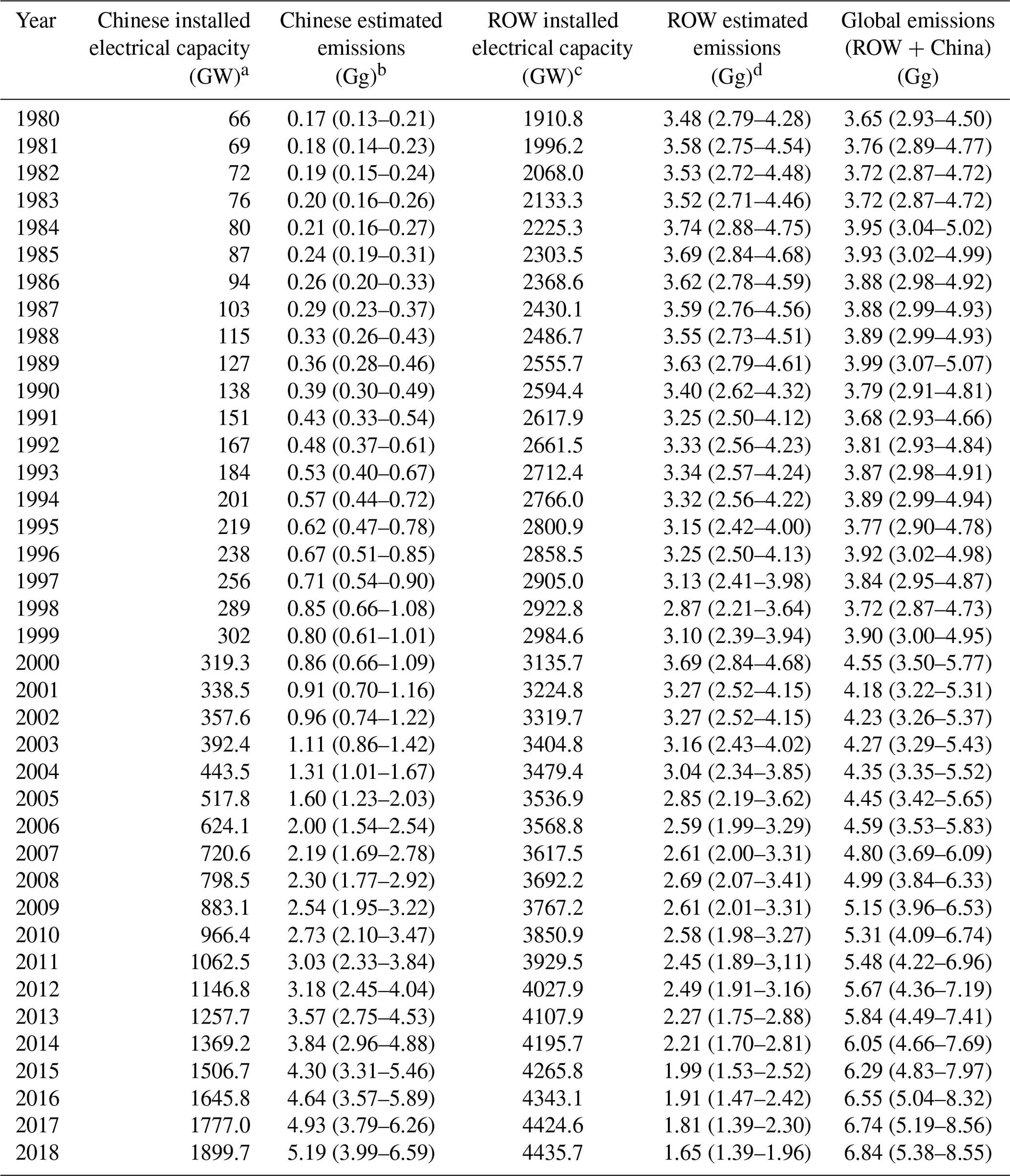
^a Chinese installed electrical power capacity compiled from https://www.statista.com/statistics/302269/china-installed-power-generation-capacity (last access: 20 December 2019) and https://www.iea.org/ (last access: 12 January 2020; IEA, 2017). ^b Estimated Chinese emissions derived from method by Zhou et al. (2018), using an initial filling of 52 t GW⁻¹ (in parenthesis, range 40–66 t GW⁻¹) and emission factors of 8.6 % (manufacture and installation) and 4.7 % (operation and maintenance). ^c Rest of the world (ROW) installed electrical power capacity is compiled from https://unstats.un.org/unsd/energystats/pubs/eprofiles (last access: 10 January 2020) (https://www.iea.org/reports/electricity-information-2019, last access: 4 December 2019) and http://mecometer.com/ (last access: 10 January 2020). ^d ROW emissions estimated using an initial filling of 52 t GW⁻¹ and a 12 % loss during manufacture and installation of new equipment and assuming 3 % loss from banked SF₆ in electrical equipment in 1980 and then decreasing linearly to 1.0 % in 2018, reflecting the change from older to newer equipment (Olivier and Bakker, 1999).

3.1.2 Magnesium industry

In the magnesium industry (dye casting, sand casting, and recycling), where SF₆ is used as a cover or blanketing gas to prevent oxidation, it is assumed that emissions are equal to consumption and all the SF₆ historically used in the magnesium industry has been emitted (https://www.ipcc-nggip.iges.or.jp, last access: 24 November 2019). The consumption of SF₆ in magnesium production in China was apparently halted after 2010 and largely replaced with SO₂ (National Bureau of Statistics, 2017). Average annual sales of SF₆ to the magnesium industry were estimated to be ∼0.25 Gg yr⁻¹ from 1996 to 2003 (Smythe, 2004). Given current regulations, the availability of substitute blanketing gases, and the assumption that Chinese and Russian producers use SO₂ as the preferred blanketing gas, we assume that current emissions from the magnesium industry are equal to or less than the 1996–2003 average of about 0.25 Gg yr⁻¹.

3.1.3 Aluminium industry

For the aluminium industry, historical emissions of SF₆ are poorly understood, as it is generally assumed to be largely destroyed during the production process by reaction with the aluminium (Victor and MacDonald, 1998); nevertheless, any surviving SF₆ will clearly be emitted (IPCC, 1997). Maiss and Brenninkmeijer (1998) roughly quantified SF₆ consumption from aluminium degassing (USA and Canada) and SF₆-insulated windows (Europe, predominately Germany) as well as numerous small specialised applications to about 450 t yr⁻¹ in 1995. Since the use of SF₆ in these applications has been substantially reduced or eliminated in the Annex-1 countries, we assume that current global emissions primarily from aluminium degassing are unlikely to be greater than 0.2 Gg yr⁻¹.

3.1.4 Electronics industry

Sulfur hexafluoride is used as a general etching agent in the electronics and semiconductor industry including the production of thin-film transistor liquid crystal displays (TFT-LCDs) and in the cleaning of chemical vapour deposition (CVD) chambers. Fang et al. (2013) reported emissions of 0.15 Gg in 2005 and 0.4 Gg in 2010 from the semiconductor industry, which has rapidly expanded in China, and emissions from this industry were reported to be 0.2–0.25 Gg yr⁻¹ during 2004–2011 (Cheng et al., 2013). Also annual average consumption by the semiconductor industry from 2012 to 2018 was reported to be 0.51 Gg yr⁻¹ (range 0.41–0.55 Gg) (World Semiconductor Council, 2020). Due to commercial confidentiality, there is very little information on the consumption of SF₆ in electronics manufacturing. However, Asian electronics industries, which dominate TFT-LCD production, have adopted substitute gases, mainly nitrogen trifluoride (NF₃), carbon tetrafluoride (CF₄), and HFC-134a (CH₂FCF₃) in preference to SF₆ in recent years. We therefore assume that global emissions of SF₆ from these industries are in the range of 0.15–0.55 Gg yr⁻¹ in the absence of any new information.

3.1.5 Production of SF₆

We also need to consider losses of SF₆ that occur during production. Fugitive emissions during SF₆ production were estimated to be 0.5 % for developed countries (IPCC, 2006). Chinese SF₆ production accounts for ∼50 % of global production and Fang et al. (2013) suggested an EF of 2.2 % (1.7–3.3 %) for China. We use these EFs for China and an EF of 0.5 % for the rest of the world to estimate an average annual SF₆ loss from production of ∼0.1 Gg yr⁻¹ (1990–2018).

The combined emissions from SF₆ production, magnesium, aluminium, and electronics industries estimated above are approximately 1.1 Gg yr⁻¹, which are prone to large uncertainties. This assumes an electronics emission of 0.55 Gg yr⁻¹, which is the highest reported by the World Semiconductor Council.

4 Top-down global emission estimates

Global emissions were derived using a two-dimensional box model of the atmosphere and a Bayesian inverse method. The AGAGE 12-box model has been used extensively for global emissions estimation and is described in Cunnold et al. (1978, 1983) and Rigby et al. (2013). The model solves for advective and diffusive fluxes between four zonal average “bands” – separated at 30^∘ N, 30^∘ S, and the Equator – and between three vertical levels separated at 500 and 200 hPa. A Bayesian inverse modelling approach was adopted that constrained the emission growth rate a priori, as described in Rigby et al. (2011, 2014) and used most recently to derive SF₆ emissions in Engel et al. (2019). Briefly, the approach assumed a priori that emissions did not change from one year to the next, with a Gaussian 1σ uncertainty in the emission growth rate set to 20 % of the maximum EDGAR v4.2 emissions. The inversion then uses an analytical Bayesian method to find a solution that best fits the observations and this prior constraint. This approach was chosen so that independent constraints on absolute emission magnitudes (e.g. as in Rigby et al., 2010), which were not available for the entire time period, were not required. Following Rigby et al. (2014), uncertainties applied to the in situ data were assumed to be equal to the variability in the monthly baseline data points, representing the sum of measurement repeatability and a model–data “mismatch” term parameterising the inability of the model to resolve sub-monthly timescales. For the archive air data, this mismatch uncertainty was taken to have the same relative magnitude as the average mismatch error found during the in situ data period. This term was added to the estimated measurement repeatability of the archive air samples. The influence of these uncertainties, and those of the prior constraint, was propagated through to the a posteriori emissions estimate; the uncertainty was augmented by an additional term representing the uncertainty in the calibration scale (2 %, applied as described in Rigby et al., 2014).

Regional emission estimates using the UK Met Office (InTEM), Empa (EBRIS), and Urbino (FLITS) inverse modelling frameworks

Three different inverse methods – (1) Inverse Technique for Emission Modelling (InTEM); (2) Swiss Federal Laboratories for Materials Science and Technology (Empa) Bayesian Regional Inversion System (EBRIS); (3) FLexpart Inversion iTalian System (FLITS), Urbino, Italy – and two different chemical transport models were used to estimate regional SF₆ emissions. A brief description of the three inverse methods is given below and a more detailed description of the InTEM and EBRIS models is provided in the Supplement.

InTEM. Arnold et al. (2018) uses the NAME (Numerical Atmospheric dispersion Modelling Environment, v7.2) (Jones et al., 2007) atmospheric Lagrangian transport model. NAME is driven by reanalysis 3-D meteorology from the UK Met Office Unified Model (Cullen, 1993). We provide estimated emissions for western Europe (UK, Ireland, Benelux countries (Belgium, the Netherlands, and Luxembourg), Germany, France, Denmark, Switzerland, Austria, Spain, Italy, and Portugal) and, in a separate analysis, emission estimates for China, using observations recorded at the Gosan station on Jeju Island, South Korea (33^∘ N, 126^∘ E). Gosan receives air masses mainly from eastern mainland China during the winter months, with winds from the north-north-west (Rigby et al., 2019; Fang et al., 2013). We subsequently scale SF₆ emissions to a Chinese total by population.

EBRIS. Henne et al. (2016) employs source sensitivities as derived from the Lagrangian particle dispersion model FLEXPART (version 9.1; Stohl et al., 2005) and observed atmospheric concentrations to optimally estimate spatially resolved surface emissions to the atmosphere. Here, EBRIS was applied to western Europe and provided country/region estimates of a posteriori SF₆ emissions.

FLITS. Another modelling approach has been used for a regional inversion. The model is based on an inversion approach developed by Stohl et al. (2005). The modelling cascade is composed of the Lagrangian particle dispersion model (LPDM) FLEXPART v9.1 (https://www.flexpart.eu/, last access: 13 May 2019) in conjunction with in situ high-frequency observations from four atmospheric monitoring sites and a Bayesian inversion technique. Here, FLEXPART was driven by operational 3-hourly meteorological data from the European Centre for Medium-Range Weather Forecasts (ECMWF) at $\mathrm{1}{}^{\circ }\times \mathrm{1}{}^{\circ }$ latitude and longitude resolution, from 2013 to 2018. We run the model in backward mode, releasing 40 000 particles from each measurement site every 3 h and followed backward in time for 20 d. Due to the long atmospheric lifetime of SF₆, the model simulation does not account for an atmospheric removal process. For the western European a priori emission field, we disaggregated 2 kt yr⁻¹ of SF₆ emissions within each country's borders according to a gridded population density data set (CIESIN, Center for International Earth Science Information Network, https://www.ciesin.org, last access: 12 November 2019), and we set 200 % of uncertainty of the emissions for every grid cell. Parameterisation details used here are described in Graziosi et al. (2015).

In Table 2 we provide details of the East Asian setup of the inversion system (InTEM), and in Table 3 we provide details of the European setup of the inversion systems (InTEM, EBRIS, FLITS).

Table 2 The East Asian setup of the inversion system runs 2007–2018 in 2-year blocks: the meteorology, atmospheric transport model (ATM), and geographical domains over which the ATM is run; the number of particles released; the inversion time steps; prior information; and observations used.

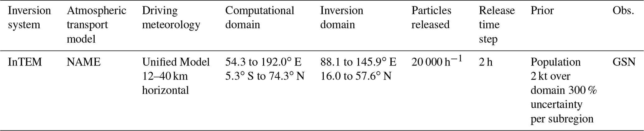
GSN: Gosan station, South Korea.

Table 3 The European setup of each inversion system run each year during 2013–2018: the meteorology, atmospheric transport model (ATM), and geographical domains over which the ATMs are run; number of particles released; inversion time steps, prior information; and observations used.

Observing stations: MHD (Mace Head, Ireland), JFJ (Jungfraujoch, Switzerland), CMN (Monte Cimone, Italy), TAC (Tacolneston, UK), RGL (Ridge Hill, UK), BSD (Bilsdale, UK), and HFD (Heathfield, UK).

5 Results

Figure 1 and Table 4 shows the AGAGE SF₆ mole fractions from 1978 to 2018, averaged into semi-hemispheres. In the lower panel of Fig. 1, we report the annual SF₆ growth rate increasing from 0.097±0.013 pmol mol⁻¹ yr⁻¹ in 1978 to reach an early maximum average growth rate in 1995 of 0.24±0.01 pmol mol⁻¹ yr⁻¹. (A Kolmogorov–Zurbenko filter was used to estimate annual mean growth rates, as described in Rigby et al., 2014.) The growth rate then gradually drops to 0.19±0.01 pmol mol⁻¹ yr⁻¹ in 2000, before increasing to reach 0.36±0.01 pmol mol⁻¹ yr⁻¹ in 2018. Between 1978 and 2018, the SF₆ loading of the atmosphere has increased by a factor of about 15. Assuming a radiative efficiency of 0.57 W m⁻² nmol mol⁻¹ (WMO, 2018), SF₆ contributed around 5.5±0.1 mW m⁻² in 2018 to global radiative forcing. In the Supplement (Fig. S1), we show the model–measurement comparison for the AGAGE 12-box model.

Table 4 Global SF₆ mole fraction output from the AGAGE 12-box model.

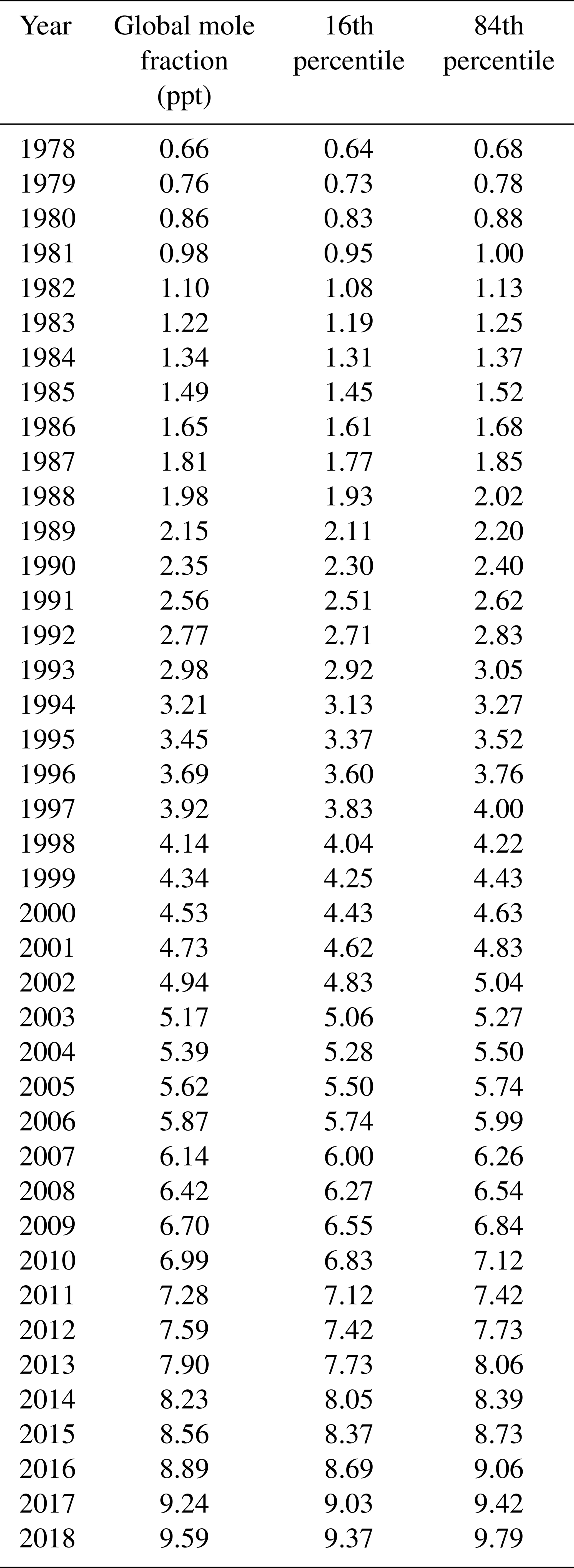
Note: mole fractions are reported at the mid-point of the year.

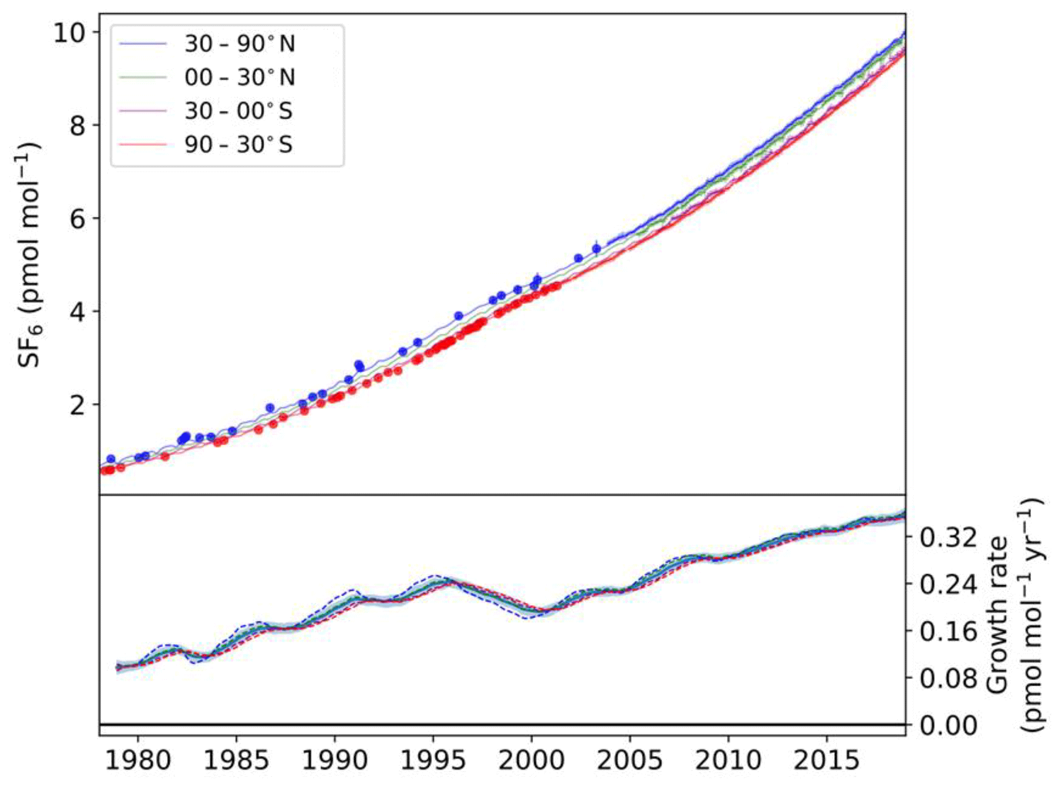
Figure 1 Observed and model-derived SF₆ mole fractions and annual growth rates from the AGAGE 12-box model. Upper panel shows measured atmospheric SF₆ mole fractions in each semi-hemisphere (points with 1σ error bars) and archived air samples collected from 1978 in the NH (blue-filled circles) and archived air samples collected at Cape Grim, Tasmania, in the SH (red-filled circles). Solid lines indicate modelled mole fractions using the mean emissions derived in the global inversion. Semi-hemispheric averages for both the model and data are shown for 30–90^∘ N (blue), 0–30^∘ N (green), 30–0^∘ S (purple), and 90–30^∘ S (red). The lower panel shows the model-derived growth rate, smoothed with an approximately 1-year filter, for each semi-hemisphere (dotted lines) and the global mean and its 1σ uncertainty (solid line and shading, respectively).

Our model-estimated annual global emissions are shown in Fig. 2 and listed in Table 5. Here we extend and update the emission estimates prior to 2008, previously described in Rigby et al. (2010), that reported a global SF₆ emission rate of 7.3±0.6 Gg yr⁻¹ (1σ uncertainty unless specified otherwise) in 2008, and Engel et al. (2019) estimated emissions of 8.7±0.4 Gg yr⁻¹ in 2016. We show that, during the last decade (2008–2018), emissions have increased by approximately 24 % to 9.04±0.35 Gg yr⁻¹. At 2018 levels, SF₆ emissions are equivalent to 212±8 Tg CO₂ (assuming a 100-year global warming potential of 23 500; Myhre et al., 2013). Our results demonstrate that, relative to 1978, global SF₆ emissions have increased by around 260 %, with cumulative global emissions through 2018 of 234±7 Gg (5500±170 Tg CO₂-equivalent). Our estimates are in close agreement through 2008 with the independent top-down estimates of Levin et al. (2010). Our estimates show similar trends to EDGAR v4.2, although our global total is on average 8.9 % higher. It should be noted that the EDGAR estimate includes some information from atmospheric observations (Rigby et al., 2010). On the other hand, it is likely that Annex-I countries are under-reporting to the UNFCCC (Weiss and Prinn, 2011) and non-Annex-I countries are not required to report to UNFCCC, which explains the much lower UNFCCC totals. There is also close agreement, within the uncertainties, of our modelled global SF₆ emission estimates and those reported by Krol et al. (2018). The annual average difference was 0.2 Gg yr⁻¹ (range 0.01–0.49 Gg yr⁻¹).

Table 5 Modelled global emissions, SF₆ emissions from China (Gg yr⁻¹), and UNFCCC reported emissions.

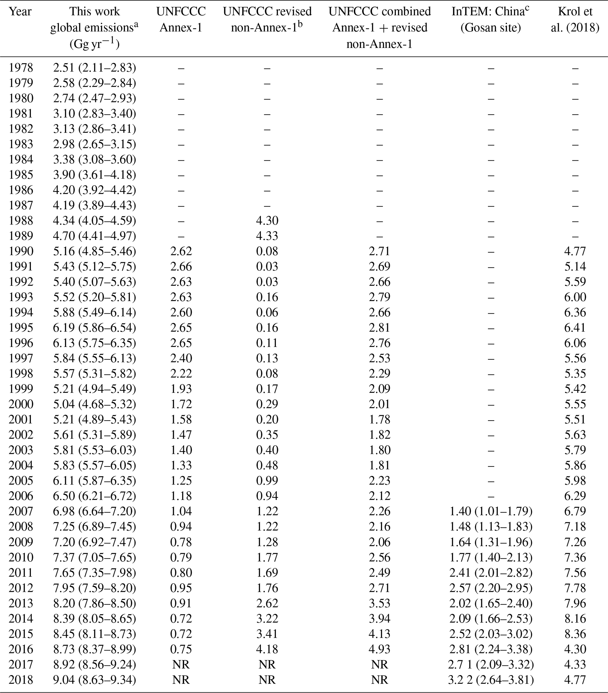
Note: uncertainties shown in parenthesis as 16th percentile and 84th percentile. NR represents “not reported”. ^a Global emissions are mid-year data. ^b Revised non-Annex-1 includes interpolated values for missing years. ^c Chinese SF₆ emissions estimated by InTEM were scaled to total Chinese emissions by population.

Figure 2 and Table 3 record the individual Annex-1 and our revised non-Annex-1 emissions and their combined emissions. UNFCCC emissions reported after 2008 for the non-Annex-1 countries exceed emissions from Annex-1 countries, as SF₆ consumption moved from Annex-1 countries to non-Annex-1 countries, particularly in Asia. We note that the significant downward trend in our top-down emission estimate between 1996 and 2000 matches the UNFCCC reported emissions; furthermore, this decline is also consistent with the drop in sales and prompt emissions listed in the RAND report (Table S2).

The average annual difference between our global top-down estimates and UNFCCC reports (Annex-1 plus revised non-Annex-1) listed in Table 5 was 4.5 Gg yr⁻¹, reaching a maximum difference of 5.2 Gg in 2012. This difference subsequently decreased to an annual average of ∼4 Gg yr⁻¹ between 2013 and 2018, implying improved or more comprehensive reporting from non-Annex-1 countries, although we recognise that these differences are prone to large uncertainties given the limited emissions data submitted to UNFCCC from the non-Annex-1 countries.

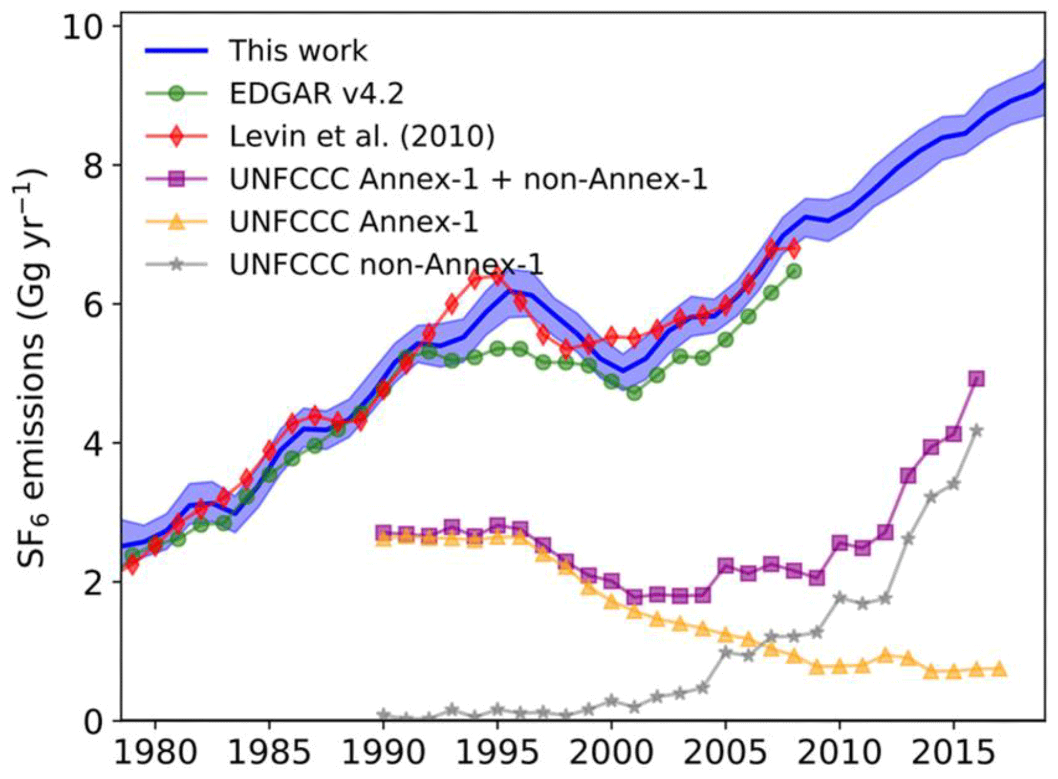
Figure 2 Optimised global SF₆ emissions using AGAGE measurements (solid blue line), and the shaded line shows the 1σ uncertainties. Emissions are from Levin et al. (2010, red diamonds), EDGAR 4.2 emissions (green circles), UNFCCC Annex-1 reported emissions (orange triangles), UNFCCC non-Annex-1 reported emissions (grey stars), and combined non-Annex-1 and Annex-1 UNFCCC emissions (purple squares).

5.1 Regional emission estimates

Top-down regional emission estimates have been calculated for two major emission regions of the world: East Asia (China, S. Korea) and western Europe. As described below, observations from Gosan (Jeju Island, South Korea; 33.3^∘ N, 126.2^∘ E) were used to estimate the Chinese emissions, and, for Europe, observations from the UK DECC network and three European AGAGE stations were used (Mace Head, MHD, Ireland; Jungfraujoch, JFJ, Switzerland; and Monte Cimone, CMN, Italy). Figure 3 records the high-frequency mole fractions of SF₆ measured at two AGAGE sites: Mace Head, MHD, Ireland (53^∘ N, 10^∘ W), and Gosan, GSN, Jeju Island, South Korea (33^∘ N, 126^∘ E). Compared to Mace Head, the Gosan data show very large enhancements (10–30 ppt, compared to 1–2 ppt) above the background mixing ratio of ∼5–10 ppt, reflecting significant regional emissions. The Gosan enhancements are associated with the transport of polluted air masses from the north-eastern part of China, the Korean Peninsula, and Japan (Kim et al., 2010; Fang et al., 2014).

Figure 3 Atmospheric mixing ratios (pmol mol⁻¹) recorded at Mace Head, Ireland (black), printed on top of the Gosan mixing ratios, Jeju Island, South Korea (green). Elevated mixing ratios represent pollution events associated with regional emissions. GSN occasionally shows a Southern Hemisphere (SH) influence during the summer, which accounts for the cases in which GSN plots below MHD.

5.2 East Asian estimated emissions

Regional top-down estimated emissions for Eastern mainland China, inferred using InTEM and Gosan measurements, are shown in Fig. 4 and listed in Table 5. Derived Chinese emissions (from an area representing 34 % of China's population) were subsequently scaled to the whole country by population. China emissions increased from 1.4 (1.0–1.8) Gg yr⁻¹ in 2007 to 3.2 (2.6–3.8) Gg yr⁻¹ in 2018, which is an increase of 130 %. Based on the InTEM regional emission estimates, China accounted for 36 % (29 %–42 %) of our model-estimated global 2018 emissions. The InTEM results show an increasing emission from China. However, the temporary rise in the mean value in 2011–2012 needs to be understood within the context of the uncertainty estimates. It is plausible, within 1σ, that there was no enhanced emissions during this period. Higher (average 38 %, 2006–2012) emissions for China (Fang et al., 2014) have been derived using observations from three stations (Gosan, South Korea; Hateruma, Japan; Cape Ochiishi, Japan) rather than one station (Gosan), using coarser and different meteorology, a detailed spatial prior, and solved for the whole of China. Also shown in Fig. 4 are our bottom-up estimated emissions calculated from the usage of SF₆ in the electrical power industry (Sect. 3.1), following the methodology published in Zhou et al. (2018) for different filling factors (FFs of 40, 52, and 66 t GW⁻¹) and high and low emission factors (EFs). The assumed high EFs were 8.6 % (manufacture and installation) and 4.7 % (operation and maintenance) and low EFs were 1.7 % (manufacture and installation) and 0.7 % (operation and maintenance). Our bottom-up estimated emissions, using the high EFs, are generally larger than the bottom-up estimated Chinese emissions determined by Fang et al. (2013), while Chinese estimates based on the lower EFs suggested by Zhou et al. (2018) are much lower than the other Chinese emission estimates. Notably, from 2007 to 2012 the bottom-up estimates, after Zhou et al. (2018), with a FF of 52 t GW⁻¹ and high EF are in close agreement with the top-down estimates by Fang et al. (2014), They also agree with our results within uncertainties. However, after about 2014 the increase in these bottom-up estimates especially with the highest FF (66 t GW⁻¹) appears to represent an unrealistically large percentage of global emissions.

The Chinese inventory compiled from biennial submissions to the UNFCCC National Communications and Biennial Update Report (2019) are also included in Fig. 4 (black-filled circles and interpolated values with grey-filled circles for missing years). Reported emissions to the UNFCCC from China, which were consistently lower than the observation-based InTEM modelled emission estimates through 2012, substantially increased in 2014 to within the uncertainties of the modelled emissions.

Figure 4 Bottom-up and top-down emission estimates scaled for the whole of China.

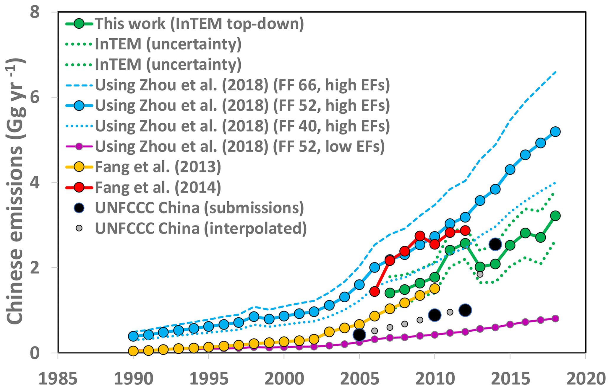
Top-down Chinese emission estimates (Fang et al., 2014) agree, within the uncertainties, with our bottom-up emission estimates. Conversely, our top-down InTEM Chinese emission estimates fall between our bottom-up and the Fang et al. (2013) bottom-up emission estimates. Regardless of the EF used, our bottom-up emission estimates would require lower Chinese EFs to obtain closer agreement with our top-down emission estimate.

Figure 5 shows the footprint of the mapped Chinese emission magnitudes determined from InTEM, based on measurements recorded at the Gosan station, South Korea. Although our main focus has been on emissions from China, it is clear from Fig. 5 that there are also emissions from South Korea. The 2007–2018 average annual SF₆ InTEM emission estimate for South Korea (population ∼52 M) is 0.26±0.05 Gg yr⁻¹ with a slight upward trend (+0.007 Gg yr⁻²). This compares well with the reported average value of 0.36 Gg yr⁻¹ over the period 2007–2014 with an upward trend of +0.006 Gg yr⁻² (South Korea, 2017, second biennial report). The emissions for South Korea are higher per head of population (∼0.005 Gg per million people) than those estimated for China (population ∼1400 million people, ∼0.002 Gg per million people in 2018). For western Europe, discussed in the next section, the equivalent value is ∼0.001 Gg per million people.

In Table S3 we list the InTEM SF₆ emission estimates for South Korea. The average annual emissions of South Korea (0.26 Gg yr⁻¹) are similar to those of western Europe (0.22 Gg yr⁻¹) and in both cases are approximately one-tenth of Chinese average annual emissions (2.2 Gg yr⁻¹).

Figure 5 Map of the top-down emission estimate from China and East Asia. The red line indicates the boundary of the region we denote “eastern mainland China”, to which the measurements at Gosan and the inversion method are most sensitive.

5.3 Western Europe emission estimates

InTEM estimated top-down emissions (2013–2018) for western Europe (United Kingdom, Ireland, Benelux, Germany, France, Denmark, Switzerland, Austria, Spain, Italy, and Portugal) from measurements at seven sites (Mace Head (MHD), Ireland; Bilsdale (BSD), UK; Heathfield (HFD), UK; Ridge Hill (RGL), UK; Tacolneston (TAC) UK; Jungfraujoch (JFJ), Switzerland; and Monte Cimone (CMN), Italy) are presented in Fig. 6 and listed in Table 6. EBRIS used observations from four sites (MHD, TAC, JFJ, CMN) to estimate top-down emissions for the period 2013–2018. Emissions from the InTEM and EBRIS inversion models are in close agreement with inventory emissions (UNFCCC 2019). FLITS also used observations (2013–2018) from four sites (MHD, TAC, JFJ, CMN) and an inverse model to estimate top-down emissions, which are higher than the other two results but follow a similar trend. The emission flux uncertainty decreases from 200 % for the a priori emission field to ∼25  % for the a posteriori emission field (average over the study period), supporting the reliability of the results. Top-down emissions for western Europe from 4 inversion systems for the year 2011 were reported to be 47 % higher than UNFCCC, with Germany identified as the principal emitter (Brunner et al., 2017).

Table 6 SF₆ emission estimates for western Europe: UNFCCC inventory, InTEM, EMPA, and FLITS emissions (Gg yr⁻¹). (Uncertainties in parenthesis.)

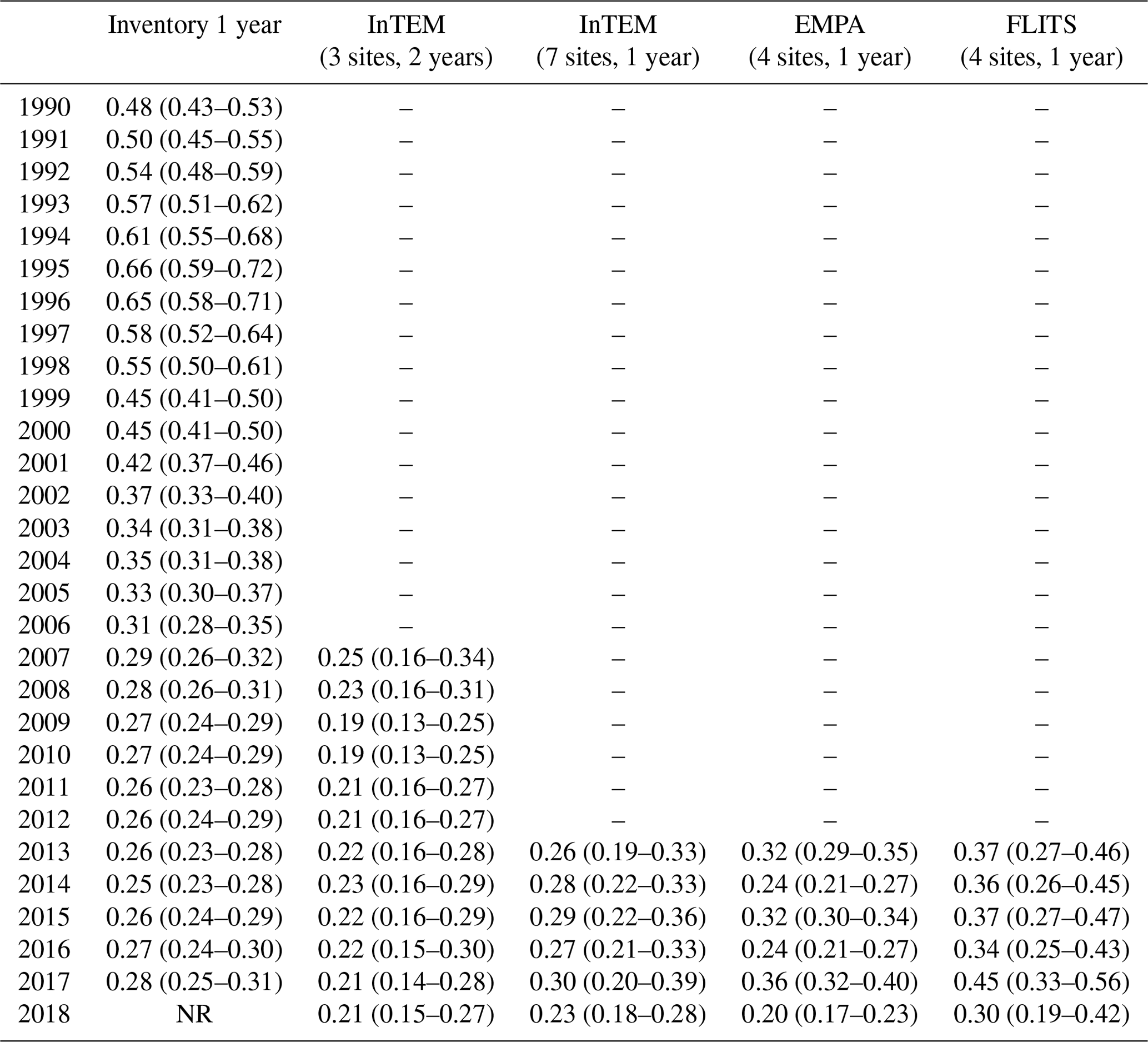
NR: not reported.

The contribution of western European SF₆ emissions to the global total in 2018 was 3.1 % (2.4–3.9 %, Table 6, average of all inversions). Comparing the model-estimated SF₆ emissions from western Europe and China, it is apparent that China is a much larger contributor to the global SF₆ inventory. On an annually averaged basis, top-down Chinese emissions exceed those emitted from western Europe by a factor of ∼10. For western Europe, EFs are generally expected to be lower, representing better maintenance practices and more efficient SF₆ capture during re-filling (EU Commission, 2015). The faster uptake of SF₆ substitutes and vacuum-insulated units would also explain the much lower emission estimates in western European countries.

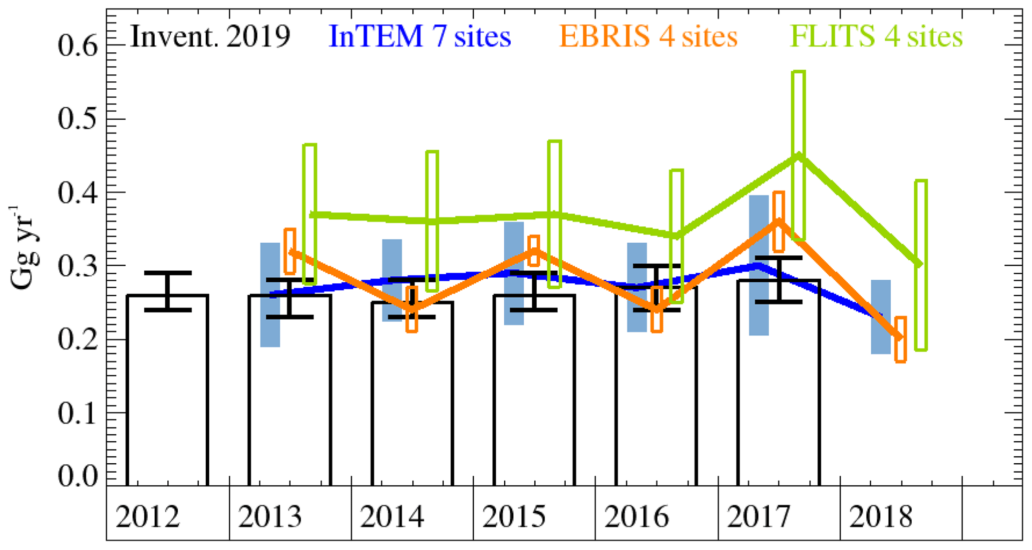
Figure 6 SF₆ western Europe emission estimates (Gg yr⁻¹) from the UNFCCC inventory (black); InTEM inversion (2013–2018, blue, seven sites: MHD, JFJ, CMN, TAC, RGL, HFD, BSD); EBRIS (2013–2018, orange, 4 sites: MHD, TAC, JFJ, CMN); and FLITS (2013–2018, green, four sites: MHD, TAC, JFJ, CMN). The uncertainty bars are ±1 SD.

Figure 7 shows the footprint of the average emission estimates for western Europe calculated using three inverse models (InTEM, EBRIS, and FLITS), illustrating that significant emissions are located in southern Germany, a region with a substantial number of semiconductor producers (https://prtr.eea.europa.eu/#home, last access: 25 November 2019).

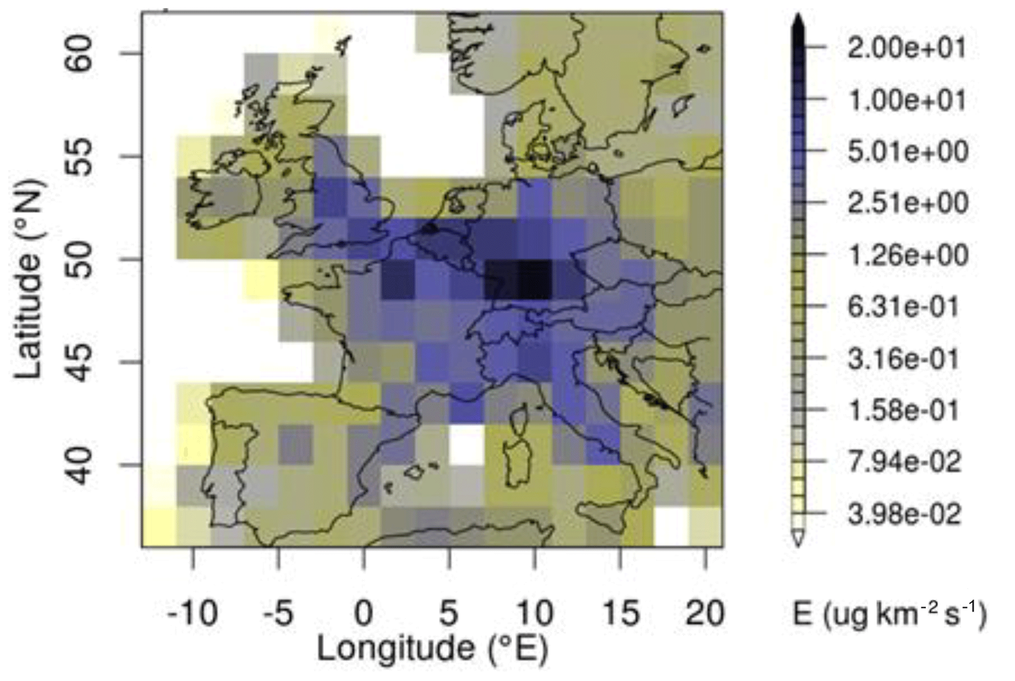
Figure 7 Top-down inversion emission estimate for western Europe (2013–2018). Average of InTEM (seven observation sites), EBRIS (four observation sites), and FLITS (four observation sites).

6 Increasing global SF₆ emissions and the deficit between bottom-up and top-down emission estimates

Weiss and Prinn (2011) noted that SF₆ bottom-up estimates derived from industrial accounting and reported to the UNFCCC by Annex-1 countries are likely under-reported, actually representing 80 % of the total in the mid-1990s and 60 % of the total in 2006, leading to poor agreement (under-reported by a factor of 2) with top-down emission estimates determined from atmospheric observations. However, for western Europe (Sect. 5.3) our estimated emissions (2013–2018) from the model inversions are in close agreement with the UNFCCC reported inventory. Limitations imposed by commercial secrecy and the lack of consistent reporting of SF₆ emissions, both from Annex-1 and non-Annex-1 countries, continue to contribute to the discrepancies between bottom-up and top-down methods.

We next explore if the increasing global emissions of SF₆ may be related to changing patterns of source location and usage in electrical equipment, magnesium smelting, aluminium production, and electronics manufacturing, and we attempt to reconcile the large average annual discrepancy of ∼4.5 Gg yr⁻¹ between bottom-up and top-down emissions estimates.

Previous reports on SF₆ emissions from the electrical power industry have noted that emission factors (EFs) may vary widely depending on the type of equipment and different maintenance and servicing practices (CAPIEL/UNIPEDE, 1999). About 12 % of SF₆ consumed in the manufacture and commissioning of electrical equipment is estimated to be directly emitted. Industry assessments of the maximum leakage during operation from older equipment (manufactured before 1980) was 3 % yr⁻¹, although higher leakage rates for some countries continued into the 1990s. For example, in 1995 USA annual refill and leakage of circuit breakers was estimated to be 20 % of total installed stock; however, with the installation of improved self-contained equipment, leakages steadily reduced from 0.5 % yr⁻¹ to 1 % yr⁻¹ (Olivier and Bakker, 1999). A recent study of the SF₆ losses from gas-insulated electrical equipment in the UK calculated an average annual leakage rate of 0.46 % yr⁻¹ from the inventory of SF₆ held in the installed equipment and 1.29 % yr⁻¹ from the transmission network, with an overall average (2010–2016) leakage rate of 1 % yr⁻¹ from the UK electrical power industry (Widger and Haddad, 2018).

Figure 8 shows the global installed electrical capacity and the percentage contribution of wind and solar power capacity from 2000 to 2018. Installed electrical capacity grew by 62 % (2412 GW) during this period. Of this rise, ∼45 % was due to solar and wind, illustrating the very rapid growth rate of the renewable sector, as utility companies invested in renewable energy (GWEC, 2018; CWEA, 2017; IRENA, 2019). The inset panel records the percentage of solar and wind power by country during 2017 – led by China, USA, and Germany. The global adoption of renewable technologies, especially hydroelectric, wind, and solar power, has been particularly strong in the non-Annex-1 countries to support their continuing development (Fang et al., 2013). For example, Chinese installed electrical capacity, relative to the ROW, increased from about 3 % in 1980 to ∼43 % in 2018, as noted in Table 1.

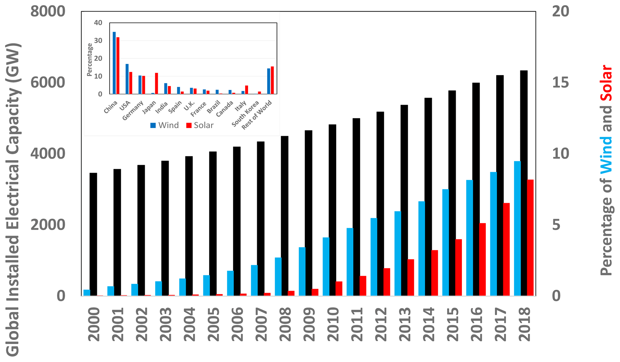
Figure 8 Global installed electrical capacity (GW) and the percentage contribution from wind power (blue bars) and solar power (red bars) from 2000 to 2018. Inset: percentage of wind and solar power by country in 2017 (IRENA, 2019).

We assume that with the wider geographical distribution of renewables, compared with the localised gas or oil-fired power stations, this has resulted in many more connections to the electricity grid and a consequent rise in the number of gas-insulated electrical switches, circuit breakers, and transformers. With the adoption of more technologically advanced gas-insulated switchgear (GIS) with lower emissions, we might expect there to be a reduction in overall SF₆ emissions over time. There is clearly a balance between the very substantial increase in the global number of newly installed GIS equipment and the major advances in reducing the leakage of SF₆ from GIS equipment and the recovery and substitution of SF₆. At present the larger number of global GIS installations appears to be overpowering the success in reducing SF₆ emissions.

Sulfur hexafluoride in the electrical power industry is primarily used in high-voltage gas-insulated switchgear (GIS), which consumes >80 % of the SF₆ used, with medium-voltage GIS consuming only about 10 % (Niemeyer and Chu, 1992; Dervos and Vassiliou, 2000; Xu et al., 2011; Xiao et al., 2018). Since this electrical equipment can be operational for 30–40 years, there is a large bank of SF₆ in older equipment that will be a continuing source of global SF₆ emissions through routine maintenance, decommissioning, catastrophic failure of components (as noted previously), and long-term leakage. Sulfur hexafluoride is also used by the utility companies in gas-insulated transmission lines (ECOFYS and ETH, 2018).

Recently, regulations have been introduced to mitigate the environmental impact of SF₆ emissions. The European Commission reinforced a 2006 F-gas regulation in 2015 (no. 517/2014) with the aim of reducing the EU's F-gas emissions by two-thirds from 2014 levels by 2030 (EU Commission, 2015). It is important to realise that under these current European regulations there are no restrictions on the use of SF₆ in switchgear, but there are requirements to recover SF₆ where possible (Biasse, 2014). Historically, SF₆ has been the preferred insulator and arc-quenching gas, although technological advances and alternative gases to SF₆ have been introduced to reduce overall emissions. Substitute gases include perfluoroketones, perfluoronitriles, and trifluoroiodomethane (CF₃I) (Okubo and Beroual, 2011; Li et al., 2018; Xiao et al., 2018). Some wind turbine manufacturers have recently started to offer SF₆-free equipment or vacuum-insulated switch gear. In 1995 the U.S. Environmental Protection Agency (EPA) established an SF₆ emissions reduction partnership for electric power systems to improve equipment reliability and reduce SF₆ emissions by technological innovation. They subsequently reported that by 2016 there had been a 74 % reduction of SF₆ emissions by the industrial partners (EPA, 2018).

The combined bottom-up emission estimated in Sect. 3.1 from SF₆ production and the various industrial applications which use SF₆ is ∼1.1 Gg yr⁻¹. Sales of SF₆ to these industries are listed in the RAND report (Smythe, 2004) from 1996 to 2003 (Table S2), which does not include recent data and only covers an unspecified part of the globe, implying a potential underestimation of actual emissions. Assuming SF₆ consumption from these industries are emitted promptly (i.e. not banked), we calculate an average annual emission from 1996 to 2003 of 1.1 Gg yr⁻¹ (0.83–1.42 Gg yr⁻¹), that includes the magnesium, electronics, adiabatic, and the fraction of “other uses” that are emitted promptly. The agreement between our bottom-up estimate of industrial emissions and the estimate derived from sales are consistently lower than modelled top-down emission estimates. Even accepting these many assumptions and uncertainties, the dominant emissions are attributable to the electrical industry and its use of SF₆-insulated equipment.

We can also obtain an “effective” EF for the electrical industry by first subtracting prompt emissions from our top-down emission estimate and then calculating the amount of SF₆ required to match the remaining annual top-down emission estimate given global installed electrical capacity and an assumed FF (52 t GW⁻¹; Zhou et al., 2018). Based on this simplified method, we estimate an effective average EF of 2.5 % for the entire time period. In Fig. 9 we compare our top-down emissions estimate and a bottom-up estimate with ±25 % uncertainty (prompt emissions plus electrical industry emissions using a median FF of 52 t GW⁻¹ and the inferred effective EF). Notwithstanding some disagreement between the top-down estimate and the simple bottom-up model during certain periods (e.g. an overestimate in the early 1980s and underestimate during the 1990s), it is notable that decadal trends in SF₆ can be broadly explained by the rise in installed electrical capacity and a single effective EF. This suggests that, when considered on ∼10-year timescales, reductions in EF achieved in certain countries, through new technologies or improved GIS management, have been offset by the growth in higher-EF GIS from other parts of the world, such that the effective EF has not changed substantially on a global scale.

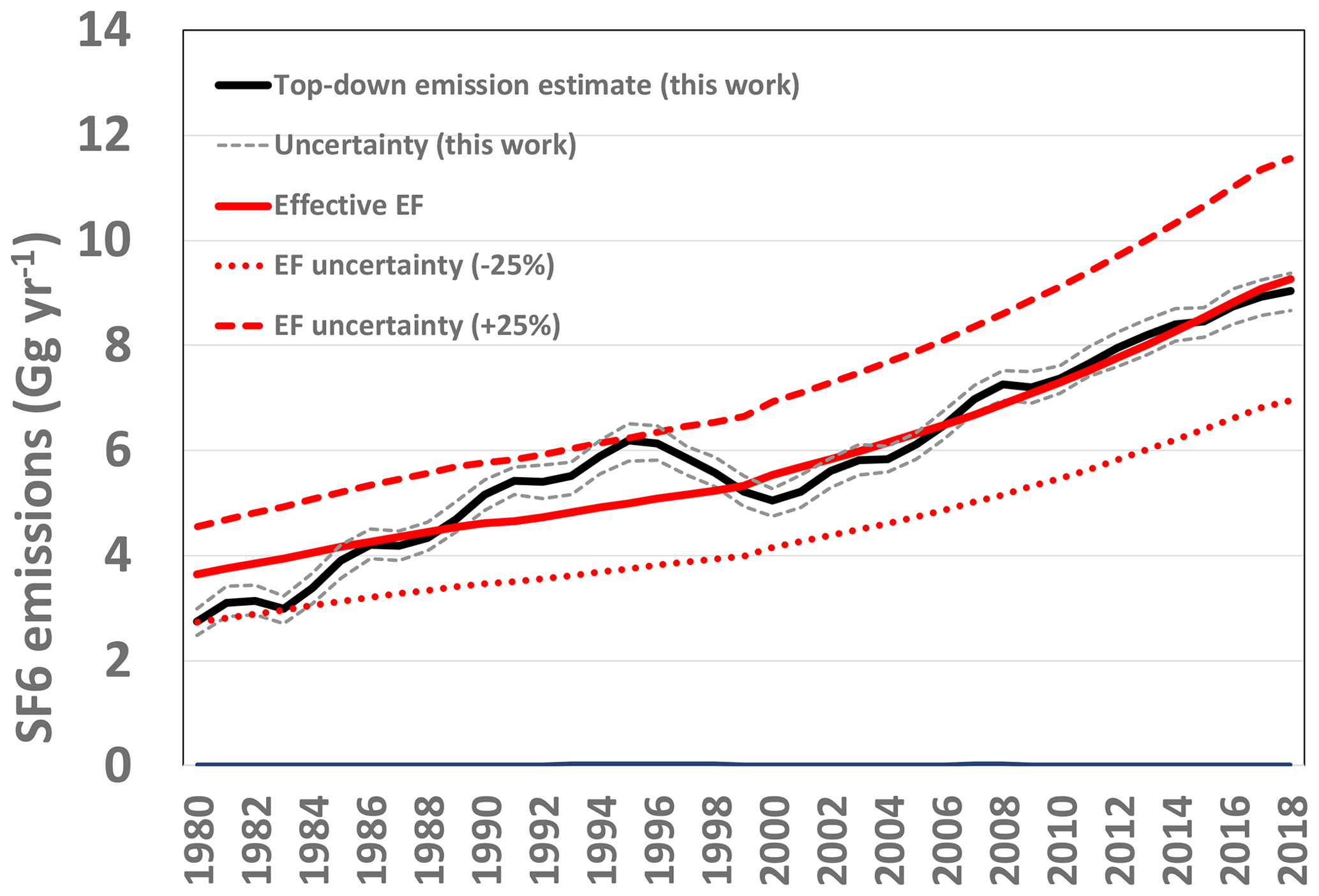
Figure 9 Top-down emission estimate (solid black line) with 1σ uncertainties and a bottom-up estimate, based on SF₆ prompt emissions plus an emissions estimate from the electrical power industry (FF=52 t GW⁻¹) and an inferred effective EF (2.5 %) with ±25 % uncertainty (dashed lines).

7 Conclusions

New atmospheric SF₆ mole fractions are presented, which extend and update our previously reported time series from the 1970s to 2008 by a further 10 years to 2018 in both hemispheres. We estimate global emissions of SF₆ using data from the five core AGAGE observing sites and archived air samples with a 12-box global chemical transport model and an inverse method. SF₆ emissions exhibited an almost linear increase from 2008–2018 reaching 9.0±0.4 Gg yr⁻¹ in 2018, a decadal increase of ∼24 %. Chinese emissions in 2018 based on InTEM regional emission estimates, with large uncertainties, account for 36 % (29 %–42 %) of total global emissions relative to our model-estimated global 2018 emissions.

We find that on an annually averaged basis emissions from China are about 10 times larger than emissions from South Korea and western Europe. Relative to 1978, global SF₆ emissions have increased by ∼260 % with cumulative global emissions through December 2018 of 234±6 Gg or CO₂ equivalents of 5.5±0.2 Pg. Further mitigating the large uncertainties will require an increase in the number of monitoring sites, improved transport models, and a substantial improvement in the accuracy and transparency of emissions reporting.

We note that the rapid expansion of global power demand and the faster adoption of renewable technologies, such as wind and solar capacity over the past decade, particularly in the Asian region, has provided a large bank of SF₆, which currently contributes to the atmospheric burden of SF₆ and will continue throughout the lifetime (30–40 years) of the installed equipment. The resultant increase in SF₆ emissions from the non-Annex-1 countries has overwhelmed the substantial reductions in overall emissions in the Annex-1 countries, where less emissive industrial practices are used in the handling of SF₆ (EPA, 2018; EU Commission, 2015). This also suggests that any decrease in emission factor from Annex-1 countries has been offset by an increase in non-Annex-1 emission factors. The non-Annex-1 countries are progressively using improved and less emissive GIS electrical equipment; however, it is only in the last few years that alternative gases to SF₆ or SF₆-free equipment have been commercially available for switchgear and other electrical systems. We conclude that the observed increase in global installed electrical capacity, in both developed and developing countries, is consistent with the temporal rise in SF₆ global emissions.