the Creative Commons Attribution 4.0 License.
the Creative Commons Attribution 4.0 License.
 | 23 Jun 2020
Effects of a priori profile shape assumptions on comparisons between satellite NO2 columns and model simulations
Randall V. Martin
Daven K. Henze
Dylan B. A. Jones
A critical step in satellite retrievals of trace gas columns is the calculation of the air mass factor (AMF) used to convert observed slant columns to vertical columns. This calculation requires a priori information on the shape of the vertical profile. As a result, comparisons between satellite-retrieved and model-simulated column abundances are influenced by the a priori profile shape. We examine how differences between the shape of the simulated and a priori profiles can impact the interpretation of satellite retrievals by performing an adjoint-based four-dimensional variational (4D-Var) assimilation of synthetic NO2 observations for constraining NOx emissions. We use the GEOS-Chem adjoint model to perform assimilations using a variety of AMFs to examine how a posteriori emission estimates are affected if the AMF is calculated using an a priori shape factor that is inconsistent with the simulated profile. In these tests, an inconsistent a priori shape factor increased root mean square errors in a posteriori emission estimates by up to 30 % for realistic conditions over polluted regions. As the difference between the simulated profile shape and the a priori profile shape increases, so do the corresponding assimilated emission errors. This reveals the importance of using simulated profile information for AMF calculations when comparing that simulated output to satellite-retrieved columns.
Please read the corrigendum first before continuing.
-
Notice on corrigendum
The requested paper has a corresponding corrigendum published. Please read the corrigendum first before downloading the article.
-
Article
(1588 KB)
-
The requested paper has a corresponding corrigendum published. Please read the corrigendum first before downloading the article.
- Article
(1588 KB) - Full-text XML
- Corrigendum
- BibTeX
- EndNote


Satellite observations provide a wealth of information on the abundance of trace gases in the troposphere (Fishman et al., 2008). The next generation of satellite instruments, including the upcoming geostationary constellation of TEMPO (Chance et al., 2013; Zoogman et al., 2017), Sentinel-4 (Bazalgette Courrèges-Lacoste et al., 2011; Ingmann et al., 2012), and GEMS (Bak et al., 2013; Kim, 2012), will provide information on NO2 and other air-quality-relevant pollutants on unprecedented spatial and temporal scales. Insight into processes that affect atmospheric composition, including emissions (Streets et al., 2013), lifetimes (Fioletov et al., 2015; de Foy et al., 2015; Laughner and Cohen, 2019), and deposition (Geddes and Martin, 2017; Kharol et al., 2018), can be gained by interpreting this information with atmospheric chemistry models.
There are three main stages in retrieving trace gas abundances from ultraviolet and visible solar backscatter radiance measurements: calculating a light-path slant column by fitting observed spectra to known spectral signatures of trace gases, removing the stratospheric portion of the column, and converting the slant column to a vertical column density using an air mass factor (AMF). AMFs are calculated using a radiative transfer model and are a function of viewing geometry, surface reflectance, clouds, and radiative transfer properties of the atmosphere. AMF calculations also require an a priori estimate of the trace gas vertical profile and are sensitive to the profile shape (Eskes and Boersma, 2003; Palmer et al., 2001). Uncertainties in AMF calculations are the dominant source of uncertainty in satellite NO2 retrievals over polluted regions (Boersma et al., 2007; Martin et al., 2002) largely due to sensitivity to surface reflectance, clouds, aerosols, and a priori profile information (Lorente et al., 2017).
Boersma et al. (2016) highlighted the issue of representativeness errors in comparing model-simulated values with UV–Vis satellite-retrieved columns. Vertical representativeness errors arise from the satellite's altitude-dependent sensitivity due to atmospheric scattering and can degrade the quality of model–measurement comparisons beyond errors that arise from either modeling or measurements alone. A consistent accounting of the altitude-dependent sensitivity is necessary to limit these errors.
Two common methods are used to account for vertical representativeness. In one method, observed slant columns are converted to vertical columns using an air mass factor calculated with scattering weights to represent instrument vertical sensitivity and shape factors to represent the vertical profile (Palmer et al., 2001). Another commonly used method employs an AMF provided with the retrieval to convert slant columns to vertical columns and then applies an averaging kernel to the simulated profile to resample the simulated profile in a manner that mimics the satellite vertical sensitivity (Eskes and Boersma, 2003). In this method both the averaging kernel and the retrieval AMF are calculated using an a priori NO2 profile that may have a different shape than the simulated profile, which may introduce errors in the observation–simulation comparison (Zhu et al., 2016).
A common application of comparisons between satellite-observed columns and model simulations is to constrain NOx emissions (e.g., Ding et al., 2018; Ghude et al., 2013; Lamsal et al., 2011; Martin et al., 2003; Vinken et al., 2014). One such approach is the use of four-dimensional variational (4D-Var) data assimilation, which seeks to minimize a cost function that accounts for the difference between simulated and retrieved values. As the cost function is a difference between observed and simulated NO2 columns, it is susceptible to vertical representativeness errors resulting from inconsistent a priori vertical profile information.
In this work we examine how a priori profile assumptions impact satellite–model comparisons and use the GEOS-Chem adjoint as a case study to assess how this impact can affect the interpretation of satellite observations. Section 2 provides the mathematical framework for AMF calculations and satellite–model comparisons. Section 3 describes the adjoint model and synthetic observations for the case study. Section 4 discusses the results.
2.1 AMFs and averaging kernels
The air mass factor translates the line-of-sight slant column abundances (Ωs) retrieved from satellite-observed radiances into vertical column abundances (Ωv). An air mass factor is the ratio of Ωs to Ωv and depends on the atmospheric path as determined by geometry, NO2 vertical profile (n), surface reflectance, and radiative transfer properties of the atmosphere. Here we use M(n) to represent an air mass factor derived using the vertical number density profile n:
In the method described by Palmer et al. (2001), a radiative transfer model is used calculate scattering weights w(z) (also known as box air mass factors) which characterize the sensitivity of backscattered radiance IB to the abundance of a trace gas at altitude z:
where αa,z is the temperature-dependent absorption cross section (m2 per molecule), αeff is the effective (weighted average) absorption cross section (m2 per molecule), and ∂τ is the incremental trace gas optical depth. MG represents a geometric path correction accounting for the satellite viewing geometry:
where θ is the solar zenith angle and θo is the satellite viewing angle. This information is then combined with an a priori NO2 shape factor (i.e., normalized vertical profile),
typically calculated with an atmospheric chemistry model to provide an air mass factor via
where S(z) is calculated using vertical profile n(z). An attribute of the formulation of Palmer et al. (2001) is the independence of atmospheric radiative transfer properties w(z) and the vertical trace gas profile S(z). The AMF definition in Eq. (1) combined with Eq. (4) indicates that a slant column can be calculated from a known vertical profile via
In an alternative formulation, the air mass factor is represented as part of an averaging kernel. As formulated by Rodgers and Connor (2003), the averaging kernel (A) provides the information needed to relate the retrieved quantity to the true atmospheric profile n:
where na is an assumed a priori profile of number density. The elements of the column averaging kernel are related to the scattering weights by
where M(na) is an air mass factor calculated using a priori vertical profile information. It is important to note that, unlike scattering weights, averaging kernels depend on the a priori assumed vertical profile shape.
A lexicon is given in Table 1 as notation used to describe these treatments has varied across the literature. We choose M for air mass factor as a single letter is clearer in equations, w for scattering weights to maintain the original formulation of Palmer et al. (2001), n for number density following IUPAC recommendations, and Ω for column densities as is common in radiative transfer literature.
Table 1Lexicon comparing notation used in this paper to that used in previous studies.
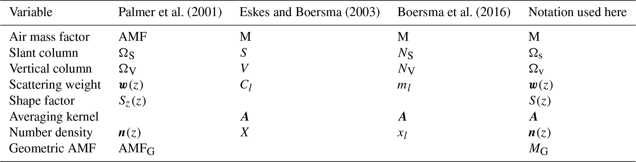
Figure 1 shows examples of typical shape factor, scattering weight, and averaging kernel profiles for a range of atmospheric conditions. NO2 shape factors have significant variability; shape factors peak near the surface in urban regions due to local pollution sources but peak in the upper troposphere in more remote regions due to lightning. The shape of a scattering weight profile depends strongly on surface reflectance and cloud conditions. Sensitivity in the lower troposphere increases over reflective surfaces. Clouds increase sensitivity above due to their reflectance but shield the satellite from observing the atmosphere below. Averaging kernels have similarities with scattering weights but depend on both the shape of the prior and the satellite sensitivity. As AMF calculations are a convolution of the shape factor and the scattering weight profiles, these shapes affect NO2 retrievals. For these examples, the AMF for a clear-sky observation with surface reflectance of 0.01 can range from 0.7 in an urban region to 1.7 in a remote region. This large difference demonstrates the importance of the assumed profile shape to the retrieval process.
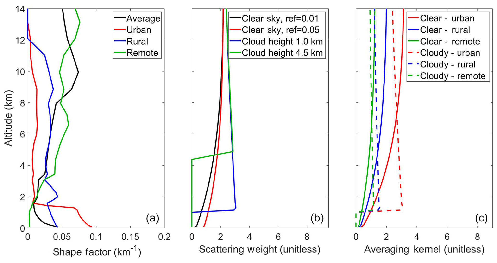
Figure 1(a) Shape factor profiles from a GEOS-Chem simulation for July 2010. Shown are a global average, as well as typical urban (Beijing), rural (Midwest USA), and remote (tropical Pacific) profiles. (b) Typical Ozone Monitoring Instrument (OMI) scattering weight profiles for varying surface reflectance and cloud height. (c) Averaging kernels calculated using the same shape factors and scattering weights (clear-sky surface reflectance is 0.01; cloudy uses a cloud height of 1 km).
2.2 Comparing satellite observations to simulated values
The following section expresses mathematically how satellite–model comparisons are made using various a priori profiles.
2.2.1 Using scattering weights
Following Palmer et al. (2001), a retrieved vertical column () is estimated using an observed slant column Ωs,o and a simulation-based air mass factor M(nm), which can be calculated with Eq. (5) using the model-simulated NO2 profile (nm):
The difference Δm between the estimated retrieved column and the model-simulated vertical column (Ωv,m) is
Equation (11) describes how this comparison is used in practice. However, we can rearrange this expression in terms of model (Ωs,m) and observed (Ωs,o) slant columns using the definition of air mass factor:
2.2.2 Using averaging kernels
Comparison of simulated and retrieved columns using the averaging kernel is described by Eskes and Boersma (2003) and in the retrieval documentation in Boersma et al. (2011). The averaging kernel is applied to the simulated profile in order to sample the simulated column in a manner that reflects the retrieval sensitivity:
The resampled simulated column is then compared to the retrieved vertical column (Ωv,o) using the a priori-based air mass factor M(na) supplied with the retrieval dataset:
Equation (16) describes how this method is used in practice. To facilitate the comparison with Eq. (13), Eq. (16) can be rewritten using an alternative formulation relating averaging kernels to scattering weights:
By comparing Eqs. (13) to (18), it is evident that the underlying difference between the two approaches is the choice of a priori profile information used to calculate the AMF, as the averaging kernel method is not independent of a priori profile assumptions. This bias could be addressed by replacing the a priori-based AMF in Eq. (18) with a simulation-based AMF using the following relationship (Boersma et al., 2016; Lamsal et al., 2010):
It should be noted that both the averaging kernel and scattering weight methods are equivalent for comparisons that examine ratios of retrieved and modeled columns:
For ratios, both methods are dependent on geophysical assumptions used to calculate scattering weights but are independent of a priori profile information. Lastly, some studies (e.g., Qu et al., 2017) may directly assimilate slant column densities rather than vertical column densities using
This approach is also still dependent upon the scattering weights but not upon external a priori profile information. Overall, the choice of approach may be influenced by whether or not scattering weights are available from either the NO2 retrieval product or radiative transfer calculations applied to the model. In contrast, use of Eqs. (11) or (16) is applicable when these are not explicitly available or provided.
3.1 GEOS-Chem and its adjoint
The GEOS-Chem chemical transport model (http://www.geos-chem.org, last access: 28 January 2020) is used to create synthetic NO2 observations and for their analysis. The GEOS-Chem version used here is version 35j of the GEOS-Chem adjoint model. GEOS-Chem includes a detailed oxidant–aerosol chemical mechanism (Bey et al., 2001; Park et al., 2004) and uses assimilated meteorological fields from the Goddard Earth Observation System (GEOS-5), with 47 vertical levels up to 0.01 hPa and a horizontal resolution of . Global anthropogenic NOx emissions are provided by the Emission Database for Global Atmospheric Research (EDGAR) inventory (Olivier et al., 2005), with regional overwrites over North America (EPA/NEI99), Europe (EMEP), Canada (CAC), Mexico (BRAVO, Kuhns et al., 2005), and East Asia (Streets et al., 2006). Other NOx sources include biomass burning (GFED2, Van der Werf et al., 2010), lightning (Murray et al., 2012), and soils (Wang et al., 1998). This model has been used previously to constrain NOx emissions (Cooper et al., 2017; Henze et al., 2009; Qu et al., 2017, 2019; Xu et al., 2013; Zhang et al., 2016).
The GEOS-Chem adjoint (Henze et al., 2007, 2009) is used here to perform a 4D-Var data assimilation. The adjoint seeks to iteratively minimize a cost function generally defined by the difference between satellite-retrieved and simulated columns (Δ, from either Eq., 11, if using a simulation-based air mass factor or Eq., 16, if using the retrieval a priori-based air mass factor):
where E and Ea are the a posteriori and a priori emissions, So and SE are the retrieval and a priori emission error covariance matrices, and γR is a regularization parameter that allows for weighting the cost function towards the retrieved columns or a priori emissions. Tests performed here required 20–30 iterations to minimize the cost function.
3.2 Experiment outline
In this study we perform 4D-Var data assimilation experiments to infer surface NOx emissions using synthetic NO2 observations. We use synthetic observations built from known emission inventories to provide a “truth” that can be used to evaluate the inversion results. To demonstrate how a priori profile information can propagate in an assimilation, we use either the model profile (Δm, Eq. 11) or an a priori profile (Δa, Eq. 16) in the cost function. A 1-week spin-up window at the start of each adjoint iteration is used to allow NOx to reach a steady state. Observation error covariances So are described as a relative error of 30 % of the slant column density plus an absolute error of 1015 molec cm−2, which is representative of typical satellite-retrieved NO2 column uncertainties (Boersma et al., 2007; Martin et al., 2002). We omit the a priori emissions constraint in the cost function (i.e., set γR=0) to isolate the impact of the observations.
3.2.1 Synthetic observations
Synthetic observations (Obs5) are created using a GEOS-Chem simulation where random Gaussian noise with a standard deviation of 5 % is added to the anthropogenic NOx emissions. Additional tests using observations where noise with a standard deviation of 30 % is added (Obs30) are also used. No additional noise is added to the individual observations to isolate the impact of AMF errors against additional sources of uncertainty. Figure 2 shows the standard (a priori) anthropogenic NOx emissions and the changes used to create the true emissions for the synthetic observations.
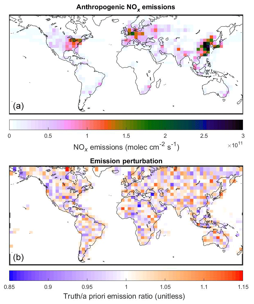
Figure 2(a) Anthropogenic NOx emissions for July 2010 used in GEOS-Chem. (b) Ratio of true emissions used to create Obs5 synthetic observations to a priori NOx emissions.
For these tests, we use one observation per hour per grid box for a period of 2 weeks in July 2010. Observations consist of synthetic slant columns (Ωs,o) created by applying scattering weights to the synthetic vertical profiles using Eq. (6). Scattering weights are calculated using the LIDORT radiative transfer model (Spurr, 2002) by providing LIDORT with the observation conditions of OMI observations during July 2010, which are used to represent typical viewing conditions of low-earth-orbit satellite observations, and aerosol profiles from the GEOS-Chem base simulation. To represent typical conditions, these representative scattering weight profiles for each grid box are used to produce the synthetic slant columns. Tests performed for all grid boxes used here indicate that the mean relative difference between an air mass factor calculated using an average scattering weight profile and the average of air mass factors using observation-specific scattering weight profiles is less than 4 %.
3.2.2 Shape factors
To test the impact of a priori profile information, seven different tests are performed using seven different NO2 profile shapes for AMF calculations:
-
Case SFM – the GEOS-Chem model-simulated profile (nm), updated at each iteration of the adjoint run.
-
Case SFprior – the a priori GEOS-Chem simulated profile, without updating.
-
Case SFn30 – an a priori profile created by a GEOS-Chem simulation where global anthropogenic NOx emissions were perturbed with random Gaussian noise with a standard deviation of 30 %; in cases where this results in negative emissions, a value of zero is used.
-
Case SFdiffem – an a priori profile created by a GEOS-Chem simulation where regional emission overwrites are turned off.
-
Case SFfiner – an a priori profile created by a GEOS-Chem simulation run at finer () resolution.
-
Case SFtrop – an a priori profile that assumes the NO2 profile shape is uniform from the surface to the tropopause (∼200 hPa).
-
Case SFBL: an a priori profile that assumes the NO2 profile shape is uniform from the surface to the boundary layer (∼800 hPa).
An advantage of using scattering weights and the simulated shape factor in a 4D-Var framework is that it allows for the shape factor, and thus the AMF, to be updated at each iteration. When a priori profiles from an external source are used it is not possible for them to update during the inversion. The SFM and SFprior cases test the impact that iterative updates to the AMF have on a posteriori estimates. The additional cases test for the impact of using an averaging kernel based on a priori profile assumptions that are inconsistent with the model. In practice, averaging kernels and a priori profiles included in retrieval datasets are generally derived from chemical transport models that have different physical processes, emissions, or spatial resolutions. The SFn30 and SFdiffem tests are representative of inversions that use a priori profile information from a different chemical transport model with similar resolution but different emissions. The SFfiner test represents an inversion that uses a priori profiles from a chemical transport model with a different horizontal resolution. The SFBLand SFtrop tests do not represent any modern retrieval algorithms but are used as extreme examples of an a priori that assumes no spatial variability. The SFBL profile is representative of polluted regions as indicated by the typical urban profile in Fig. 1, while the SFtrop profile is representative of a typical rural profile. Table 2 provides global mean AMFs for these test cases, which range from 1.3 to 2.1, and the resulting global mean observed vertical columns, which range from 0.9 to 1.5×10¹⁵ molec cm−2. Global mean observed vertical columns are 33 % higher for SF2×25 than for SFM and up to 66 % higher for SFBL. Global mean observed vertical columns for SFn30 and SFdiffem are similar to SFM, although individual observations may differ by up to 18 % for SFn30 and 28 % for SFdiffem.
Table 2Global mean air mass factors and synthetic observation vertical column density for shape factors tested here.
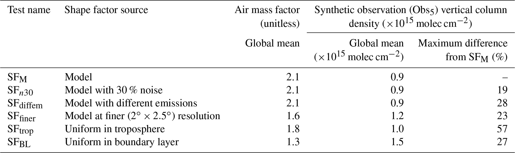
Figure 3 shows root mean square errors (RMSEs) for the a posteriori emissions estimated by the 4D-Var assimilations of Obs5 synthetic observations. All tests successfully reduce the a priori emission error by an order of magnitude or more. The SFM has the lowest RMSE, indicating that it can best estimate the true emissions. The next lowest RMSE is for the SFprior test, which uses the same initial model shape factor but does not update during the adjoint iterations, followed by the SFfiner, SFdiffem, SFn30, SFtrop, and SFBL tests.
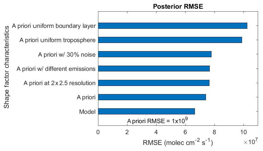
Figure 3Global root mean square error (RMSE) values for 4D-Var estimates of NOx emissions for tests using various shape factors in AMF calculations.
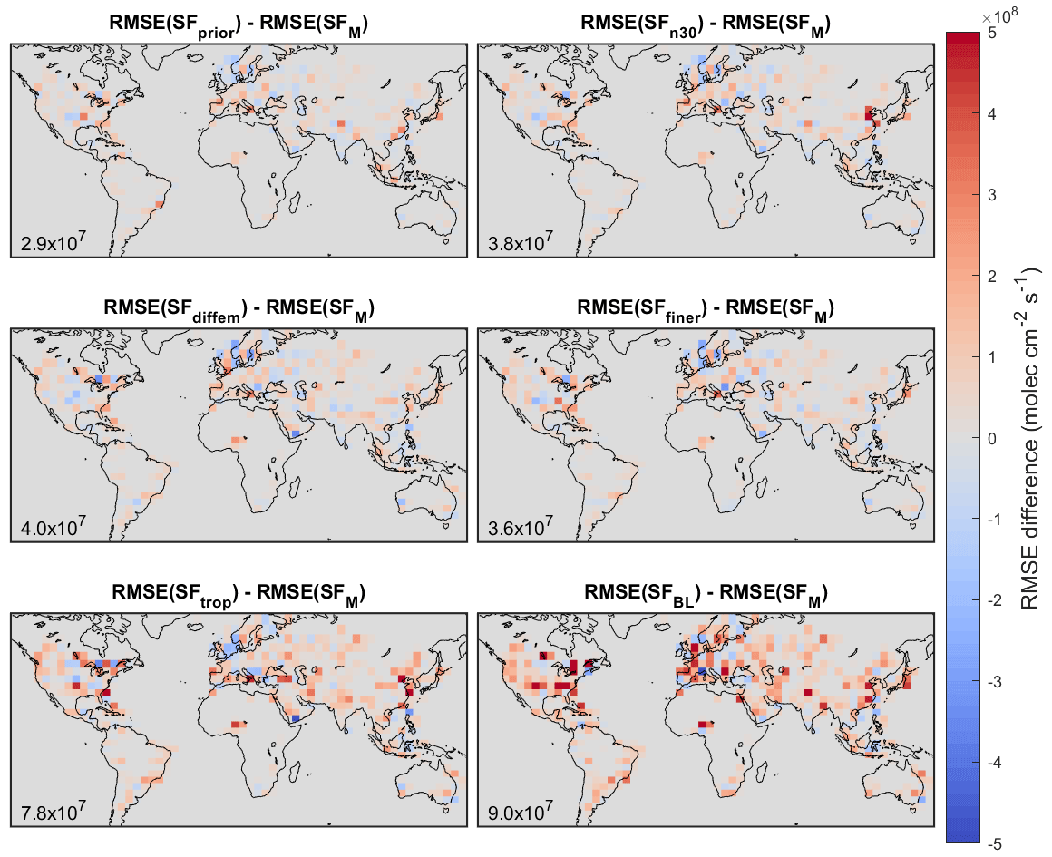
Figure 4Difference between root mean square error (RMSE) of adjoint tests for Obs5 synthetic observations. Root mean square differences between the a posteriori emissions estimates (molec cm−2 s−1) are inset.
Figure 4 shows maps of the difference in RMSE between the SFM test and the other tests for Obs5 observations. The SFM test has a lower RMSE than the other tests in 65 %–72 % grid boxes where the difference is nonzero. Again, the SFprior test is closest to the SFM test with a root mean square difference of 2.9×10⁷ molec cm−2 s−1, followed by SFfiner (3.6×10⁷ molec cm−2 s−1), SFn30 (3.8×10⁷ molec cm−2 s−1), SFdiffem (4.0×10⁷ molec cm−2 s−1), SFtrop, (7.8×10⁷ molec cm−2 s−1), and SFBL (9.0×10⁷ molec cm−2 s−1).
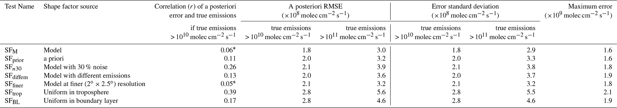
Table 3 summarizes additional error statistics focused on grid boxes with significant emission sources. Errors in a posteriori emission estimates are correlated with the true emissions in the SFtrop and SFn30 tests, and they are weakly correlated in the SFBL, SFprior, and SFdiffem tests, indicating that these tests are not constraining the emissions well. Differences between tests are more significant over polluted regions where AMF errors are more influential; for example, in the regions with the highest NOx emissions, RMSE values indicate SFM outperforms SFn30 by 30 % and SFtrop by > 80 %. Another sign of adjoint inversion quality is a low variance in errors. While the posterior error is reduced relative to the a priori error in all tests, error standard deviations are 30 % higher for SFn30 and 90 % higher for SFtrop compared to SFM. The global maximum error for the SFtrop test is 30 % higher than for the SFM test. All metrics indicate that the SFM test best represents the true emissions.
Table 3Summary of error statistics for adjoint tests. Values marked with asterisks (*) indicate that correlation is not statistically significant (p > 0.05). For comparisons, mean true emissions for grid boxes with emissions > 1010 molec cm−2 s−1 are 4.9×10¹⁰, and mean true emissions for boxes with emissions > 1011 molec cm−2 s−1 are 1.6×10¹¹ molec cm−2 s−1.
Tests using Obs30 observations and the SFMand SFtrop shape factors were also performed. Despite the difference between a priori observed vertical columns using these shape factors as indicated by Table 2, these assimilations produced similar a posteriori results, with RMSE of 2.9×10⁸ molec cm−2 s−1 for SFM and 2.8×10⁸ molec cm−2 s−1 for SFtrop.
Accounting for the vertical profile dependence of satellite observations is essential to accurately interpret those observations. This work examines how the choice of shape factor affects differences between simulated and satellite-retrieved quantities in a data assimilation framework. Examination of the mathematical frameworks behind two common methods for comparing simulated and retrieved columns highlights how the method introduced by Palmer et al. (2001) facilitates separation of observation sensitivity (scattering weights) from the profile shape (shape factor) enabling the model–retrieval comparison to be independent of a priori profile assumptions.
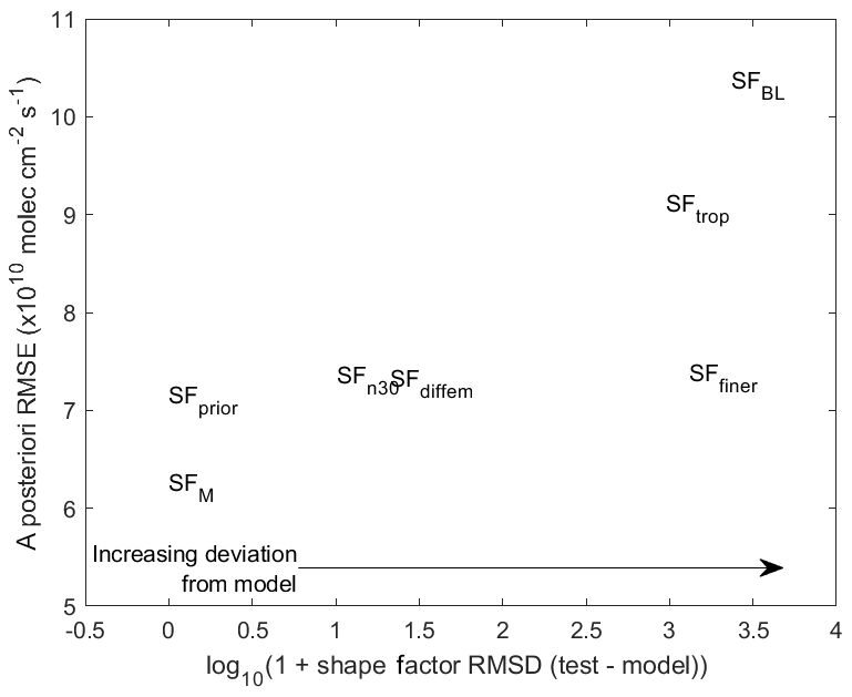
Figure 5Scatterplot of adjoint test results. X axis represents the deviation of the shape factor from the model-simulated shape factor (root mean square difference). Y axis represents the a posteriori emissions error from the adjoint inversion.
In these case studies, vertical representativeness errors were best reduced by using a shape factor that was consistent with the model simulation. This was especially true in polluted regions where the AMF errors dominate observation uncertainties, as deviations between the tests were largest in these regions. The further the shape factor deviated from the model state the larger the inversion errors became, as indicated by Fig. 5. The SFfiner test indicates that although using a finer-resolution model to generate a priori profiles is desirable for a more accurate retrieval, consistency between the simulation profile and the a priori shape factor is of greater importance explicitly for the purpose of simulation–observation comparisons to constrain emissions at the simulation resolution. Comparing the SFM and SFprior tests shows that allowing for the shape factor to update during the iterative adjoint process further reduces the RMSE by 10 %. However, even without allowing for shape factor updates, using a shape factor that is consistent with the initial model state produces a more accurate inversion result than using other assumed profile shapes.
The case study presented here demonstrates that the shape factor source can have a strong influence on adjoint inversion results. However, the magnitude of this influence can vary. Inversion tests performed using synthetic observations based on random 30 % perturbations to emissions were insensitive to the AMF, despite large differences in a priori vertical column densities. In these tests, the cost function was more sensitive to the larger difference between the observed and simulated slant columns (i.e., in Eqs. 13 and 19) than to the AMF. This indicates that while the cost function is mathematically dependent on the AMF, the inversion is less sensitive to vertical representativeness errors in cases where emissions are poorly constrained, as is the case in recent adjoint inversion studies (e.g., Qu et al., 2017). However, the choice of AMF will become increasingly important to adjoint inversions as emission inventories improve. Furthermore, omitting the a priori emissions constraint in the cost function and omitting noise in the observations in these tests to isolate the impact of the AMF effectively assume poorly constrained a priori emissions and ideal observations. In practice, cost function sensitivity to AMF choice may be buffered when a priori emissions uncertainties and observational noise are considered.
As it is beneficial for a consistent shape factor to be used when comparing satellite-retrieved values to model-simulated results, it will be useful for data products to provide the information required for this method to the user community. This is most straightforward when scattering weights (rather than averaging kernels) are provided alongside retrieved column data, as scattering weights and shape factors are independently calculated; however, simulation-based air mass factors can be calculated using the averaging kernel and a priori-based air mass factor via Eq. (19).
In summary, when comparing a model simulation to a satellite-retrieved NO2 column in a data assimilation environment utilizing column differences, calculating the AMF using the simulated shape factor allows for better accuracy in inversion results. This demonstration can provide general guidance for other methods of interpreting satellite observations with models, as using the simulated shape factor assures consistency in the vertical representativeness between model and retrieval.
The GEOS-Chem chemical transport model and its adjoint are available at http://acmg.seas.harvard.edu/geos/ (GEOS-Chem, 2017). OMI NO2 data used in this study are available from the NASA Goddard Earth Sciences Data and Information Services Center (https://doi.org/10.5067/Aura/OMI/DATA2017, Krotkov et al., 2019). AMF code (Spurr, 2002; Martin et al., 2002) used to calculate scattering weights and air mass factors is available at http://fizz.phys.dal.ca/~atmos/martin/?page_id=129 (Palmer, 2017).
MJC and RVM designed the overall study. MJC designed and carried out the case studies and their analysis. All coauthors provided guidance in analyzing results. MJC prepared the manuscript with contributions from all coauthors.
The authors declare that they have no conflict of interest.
This research has been supported by the Canadian Space Agency. Daven K. Henze was supported by NASA (grant no. NNX17AF63G).
This paper was edited by Ronald Cohen and reviewed by two anonymous referees.
Bak, J., Kim, J. H., Liu, X., Chance, K., and Kim, J.: Evaluation of ozone profile and tropospheric ozone retrievals from GEMS and OMI spectra, Atmos. Meas. Tech., 6, 239–249, https://doi.org/10.5194/amt-6-239-2013, 2013.
Bazalgette Courrèges-Lacoste, G., Ahlers, B., Guldimann, B., Short, A., Veihelmann, B., and Stark, H.: The Sentinel-4/UVN instrument on-board MTG-S, in EUMETSAT Meteorological Satellite Conference, Oslo, Norway, 2011.
Bey, I., Jacob, D. J., Yantosca, R. M., Logan, J. A., Field, B. D., Fiore, A. M., Li, Q., Liu, H. Y., Mickley, L. J., and Schultz, M. G.: Global modeling of tropospheric chemistry with assimilated meteorology: Model description and evaluation, J. Geophys. Res.-Atmos., 106, 23073–23095, 2001.
Boersma, K., Braak, R., and van der A, R. J.: Dutch OMI NO2 (DOMINO) data product v2. 0, Tropospheric Emissions Monitoring Internet Service on-line documentation, available at: http://www.temis.nl/docs/OMI_NO2_HE5_2.0_2011.pdf, last access: 19 September 2011.
Boersma, K. F., Eskes, H. J., Veefkind, J. P., Brinksma, E. J., van der A, R. J., Sneep, M., van den Oord, G. H. J., Levelt, P. F., Stammes, P., Gleason, J. F., and Bucsela, E. J.: Near-real time retrieval of tropospheric NO2 from OMI, Atmos. Chem. Phys., 7, 2103–2118, https://doi.org/10.5194/acp-7-2103-2007, 2007.
Boersma, K. F., Vinken, G. C. M., and Eskes, H. J.: Representativeness errors in comparing chemistry transport and chemistry climate models with satellite UV–Vis tropospheric column retrievals, Geosci. Model Dev., 9, 875–898, https://doi.org/10.5194/gmd-9-875-2016, 2016.
Chance, K., Liu, X., Suleiman, R. M., Flittner, D. E., Al-Saadi, J., and Janz, S. J.: Tropospheric emissions: monitoring of pollution (TEMPO), Proc. SPIE 8866, Earth Observing Systems XVIII, 88660D, https://doi.org/10.1117/12.2024479, 2013.
Cooper, M., Martin, R. V., Padmanabhan, A., and Henze, D. K.: Comparing mass balance and adjoint methods for inverse modeling of nitrogen dioxide columns for global nitrogen oxide emissions, J. Geophys. Res.-Atmos., 122, 4718–4734, https://doi.org/10.1002/2016JD025985, 2017.
de Foy, B., Lu, Z., Streets, D. G., Lamsal, L. N., and Duncan, B. N.: Estimates of power plant NOx emissions and lifetimes from OMI NO2 satellite retrievals, Atmos. Environ., 116, 1–11, 2015.
Ding, J., van der A, R. J., Mijling, B., Jalkanen, J.-P., Johansson, L., and Levelt, P. F.: Maritime NOx Emissions Over Chinese Seas Derived From Satellite Observations, Geophys. Res. Lett., 45, 2031–2037, https://doi.org/10.1002/2017GL076788, 2018.
Eskes, H. J. and Boersma, K. F.: Averaging kernels for DOAS total-column satellite retrievals, Atmos. Chem. Phys., 3, 1285–1291, https://doi.org/10.5194/acp-3-1285-2003, 2003.
Fioletov, V. E., McLinden, C. A., Krotkov, N., and Li, C.: Lifetimes and emissions of SO2 from point sources estimated from OMI, Geophys. Res. Lett., 42, 1969–1976, https://doi.org/10.1002/2015GL063148, 2015.
Fishman, J., Al-Saadi, J. A., Creilson, J. K., Bowman, K. W., Burrows, J. P., Richter, A., Chance, K. V., Edwards, D. P., Martin, R. V., Morris, G. A., Pierce, R. B., Ziemke, J. R., Schaack, T. K., Thompson, A. M., Fishman, J., Al-Saadi, J. A., Creilson, J. K., Bowman, K. W., Burrows, J. P., Richter, A., Chance, K. V., Edwards, D. P., Martin, R. V., Morris, G. A., Pierce, R. B., Ziemke, J. R., Schaack, T. K., and Thompson, A. M.: Remote Sensing of Tropospheric Pollution from Space, B. Am. Meteorol. Soc., 89, 805–821, https://doi.org/10.1175/2008BAMS2526.1, 2008.
Geddes, J. A. and Martin, R. V.: Global deposition of total reactive nitrogen oxides from 1996 to 2014 constrained with satellite observations of NO2 columns, Atmos. Chem. Phys., 17, 10071–10091, https://doi.org/10.5194/acp-17-10071-2017, 2017.
GEOS-Chem: GEOS-Chem chemical transport model, available at: http://acmg.seas.harvard.edu/geos/, last access: 20 August 2017.
Ghude, S. D., Pfister, G. G., Jena, C., van der A, R. J., Emmons, L. K., and Kumar, R.: Satellite constraints of nitrogen oxide (NOx) emissions from India based on OMI observations and WRF-Chem simulations, Geophys. Res. Lett., 40, 423–428, 2013.
Henze, D. K., Hakami, A., and Seinfeld, J. H.: Development of the adjoint of GEOS-Chem, Atmos. Chem. Phys., 7, 2413–2433, https://doi.org/10.5194/acp-7-2413-2007, 2007.
Henze, D. K., Seinfeld, J. H., and Shindell, D. T.: Inverse modeling and mapping US air quality influences of inorganic PM2.5 precursor emissions using the adjoint of GEOS-Chem, Atmos. Chem. Phys., 9, 5877–5903, https://doi.org/10.5194/acp-9-5877-2009, 2009.
Ingmann, P., Veihelmann, B., Langen, J., Lamarre, D., Stark, H., and Courrèges-Lacoste, G. B.: Requirements for the GMES Atmosphere Service and ESA's implementation concept: Sentinels-4/-5 and -5p, Remote Sens. Environ., 120, 58–69, https://doi.org/10.1016/j.rse.2012.01.023, 2012.
Kharol, S. K., Shephard, M. W., McLinden, C. A., Zhang, L., Sioris, C. E., O'Brien, J. M., Vet, R., Cady-Pereira, K. E., Hare, E., Siemons, J., and Krotkov, N. A.: Dry Deposition of Reactive Nitrogen From Satellite Observations of Ammonia and Nitrogen Dioxide Over North America, Geophys. Res. Lett., 45, 1157–1166, https://doi.org/10.1002/2017GL075832, 2018.
Kim, J.: GEMS (Geostationary Environment Monitoring Spectrometer) onboard the GeoKOMPSAT to monitor air quality in high temporal and spatial resolution over Asia-Pacific Region, in EGU General Assembly Conference Abstracts, vol. 14, p. 4051, 2012.
Kuhns, H., Knipping, E. M., and Vukovich, J. M.: Development of a United States–Mexico emissions inventory for the big bend regional aerosol and visibility observational (BRAVO) study, J. Air Waste Manage., 55, 677–692, 2005.
Lamsal, L. N., Martin, R. V., Van Donkelaar, A., Celarier, E. A., Bucsela, E. J., Boersma, K. F., Dirksen, R., Luo, C., and Wang, Y.: Indirect validation of tropospheric nitrogen dioxide retrieved from the OMI satellite instrument: Insight into the seasonal variation of nitrogen oxides at northern midlatitudes, J. Geophys. Res.-Atmos., 115, D05302, https://doi.org/10.1029/2009JD013351, 2010.
Lamsal, L. N., Martin, R. V, Padmanabhan, A., van Donkelaar, A., Zhang, Q., Sioris, C. E., Chance, K., Kurosu, T. P., and Newchurch, M. J.: Application of satellite observations for timely updates to global anthropogenic NOx emission inventories, Geophys. Res. Lett., 38, L05810, https://doi.org/10.1029/2010GL046476, 2011.
Laughner, J. L. and Cohen, R. C.: Direct observation of changing NOx lifetime in North American cities, Science, 366, 723–727, https://doi.org/10.1126/science.aax6832, 2019.
Laughner, J. L., Zare, A., and Cohen, R. C.: Effects of daily meteorology on the interpretation of space-based remote sensing of NO2, Atmos. Chem. Phys., 16, 15247–15264, https://doi.org/10.5194/acp-16-15247-2016, 2016.
Lorente, A., Folkert Boersma, K., Yu, H., Dörner, S., Hilboll, A., Richter, A., Liu, M., Lamsal, L. N., Barkley, M., De Smedt, I., Van Roozendael, M., Wang, Y., Wagner, T., Beirle, S., Lin, J.-T., Krotkov, N., Stammes, P., Wang, P., Eskes, H. J., and Krol, M.: Structural uncertainty in air mass factor calculation for NO2 and HCHO satellite retrievals, Atmos. Meas. Tech., 10, 759–782, https://doi.org/10.5194/amt-10-759-2017, 2017.
Martin, R. V., Chance, K., Jacob, D. J., Kurosu, T. P., Spurr, R. J. D., Bucsela, E., Gleason, J. F., Palmer, P. I., Bey, I., and Fiore, A. M.: An improved retrieval of tropospheric nitrogen dioxide from GOME, J. Geophys. Res.-Atmos., 107, 4437, https://doi.org/10.1029/2001JD001027, 2002.
Martin, R. V., Jacob, D. J., Chance, K., Kurosu, T. P., Palmer, P. I., and Evans, M. J.: Global inventory of nitrogen oxide emissions constrained by space-based observations of NO2 columns, J. Geophys. Res., 108, 4537, https://doi.org/10.1029/2003JD003453, 2003.
Murray, L. T., Jacob, D. J., Logan, J. A., Hudman, R. C., and Koshak, W. J.: Optimized regional and interannual variability of lightning in a global chemical transport model constrained by LIS/OTD satellite data, J. Geophys. Res.-Atmos., 117, D20307, https://doi.org/10.1029/2012JD017934, 2012.
Krotkov, N. A., Lamsal, L. N., Marchenko, S. V., Celarier, E. A., Bucsela, E. J., Swartz, W. H., Joiner, J., and the OMI core team: OMI/Aura Nitrogen Dioxide (NO2) Total and Tropospheric Column 1-orbit L2 Swath 13×24 km V003, Greenbelt, MD, USA, Goddard Earth Sciences Data and Information Services Center (GES DISC), https://doi.org/10.5067/Aura/OMI/DATA2017, 2019.
Olivier, J. G. J., Van Aardenne, J. A., Dentener, F. J., Pagliari, V., Ganzeveld, L. N., and Peters, J. A. H. W.: Recent trends in global greenhouse gas emissions: regional trends 1970–2000 and spatial distributionof key sources in 2000, Environ. Sci., 2, 81–99, 2005.
Palmer, P.: AMF code, available at http://fizz.phys.dal.ca/~atmos/martin/?page_id=129, last access: 19 June 2017.
Palmer, P. I., Jacob, D. J., Chance, K., and Martin, R. V: Air mass factor formulation for spectroscopic measurements from satellites' Application to formaldehyde retrievals from the Global Ozone Monitoring Experiment, J. Geophys. Res., 106, 14539–14550, https://doi.org/10.1029/2000JD900772, 2001.
Park, R. J., Jacob, D. J., Field, B. D., Yantosca, R. M., and Chin, M.: Natural and transboundary pollution influences on sulfate-nitrate-ammonium aerosols in the United States: Implications for policy, J. Geophys. Res.-Atmos., 109, D15204, https://doi.org/10.1029/2003JD004473, 2004.
Qu, Z., Henze, D. K., Capps, S. L., Wang, Y., Xu, X., Wang, J., and Keller, M.: Monthly top-down NOx emissions for China (2005–2012): A hybrid inversion method and trend analysis, J. Geophys. Res.-Atmos., 122, 4600–4625, https://doi.org/10.1002/2016JD025852, 2017.
Qu, Z., Henze, D. K., Theys, N., Wang, J., and Wang, W.: Hybrid mass balance/4D-Var joint inversion of NOx and SO2 emissions in East Asia, J. Geophys. Res.-Atmos., 124, 8203–8224, https://doi.org/10.1029/2018JD030240, 2019.
Rodgers, C. D. and Connor, B. J.: Intercomparison of remote sounding instruments, J. Geophys. Res.-Atmos., 108, 4116, https://doi.org/10.1029/2002JD002299, 2003.
Spurr, R. J. D.: Simultaneous derivation of intensities and weighting functions in a general pseudo-spherical discrete ordinate radiative transfer treatment, J. Quant. Spectrosc. Ra., 75, 129–175, https://doi.org/10.1016/S0022-4073(01)00245-X, 2002.
Streets, D. G., Zhang, Q., Wang, L., He, K., Hao, J., Wu, Y., Tang, Y., and Carmichael, G. R.: Revisiting China's CO emissions after the transport and chemical evolution over the Pacific (TRACE-P) mission: synthesis of inventories, atmospheric modeling, and observations, J. Geophys. Res.-Atmos., 111, D14306, https://doi.org/10.1029/2006JD007118, 2006.
Streets, D. G., Canty, T., Carmichael, G. R., De Foy, B., Dickerson, R. R., Duncan, B. N., Edwards, D. P., Haynes, J. A., Henze, D. K., Houyoux, M. R., Jacob, D. J., Krotkov, N. A., Lamsal, L. N., Liu, Y., Lu, Z., Martin, R. V., Pfister, G. G., Pinder, R. W., Salawitch, R. J., and Wecht, K. J.: Emissions estimation from satellite retrievals: A review of current capability, Atmos. Environ., 77, 1011–1042, https://doi.org/10.1016/j.atmosenv.2013.05.051, 2013.
van der Werf, G. R., Randerson, J. T., Giglio, L., Collatz, G. J., Mu, M., Kasibhatla, P. S., Morton, D. C., DeFries, R. S., Jin, Y., and van Leeuwen, T. T.: Global fire emissions and the contribution of deforestation, savanna, forest, agricultural, and peat fires (1997–2009), Atmos. Chem. Phys., 10, 11707–11735, https://doi.org/10.5194/acp-10-11707-2010, 2010.
Vinken, G. C. M., Boersma, K. F., Maasakkers, J. D., Adon, M., and Martin, R. V.: Worldwide biogenic soil NOx emissions inferred from OMI NO2 observations, Atmos. Chem. Phys., 14, 10363–10381, https://doi.org/10.5194/acp-14-10363-2014, 2014.
Wang, Y., Jacob, D. J., and Logan, J. A.: Global simulation of tropospheric O3-NOx-hydrocarbon chemistry: 1. Model formulation, J. Geophys. Res.-Atmos., 103, 10713–10725, 1998.
Xu, X., Wang, J., Henze, D. K., Qu, W., and Kopacz, M.: Constraints on aerosol sources using GEOS-Chem adjoint and MODIS radiances, and evaluation with multisensor (OMI, MISR) data, J. Geophys. Res.-Atmos., 118, 6396–6413, https://doi.org/10.1002/jgrd.50515, 2013.
Zhang, L., Shao, J., Lu, X., Zhao, Y., Hu, Y., Henze, D. K., Liao, H., Gong, S., and Zhang, Q.: Sources and Processes Affecting Fine Particulate Matter Pollution over North China: An Adjoint Analysis of the Beijing APEC Period, Environ. Sci. Technol., 50, 8731–8740, https://doi.org/10.1021/acs.est.6b03010, 2016.
Zhu, L., Jacob, D. J., Kim, P. S., Fisher, J. A., Yu, K., Travis, K. R., Mickley, L. J., Yantosca, R. M., Sulprizio, M. P., De Smedt, I., González Abad, G., Chance, K., Li, C., Ferrare, R., Fried, A., Hair, J. W., Hanisco, T. F., Richter, D., Jo Scarino, A., Walega, J., Weibring, P., and Wolfe, G. M.: Observing atmospheric formaldehyde (HCHO) from space: validation and intercomparison of six retrievals from four satellites (OMI, GOME2A, GOME2B, OMPS) with SEAC4RS aircraft observations over the southeast US, Atmos. Chem. Phys., 16, 13477–13490, https://doi.org/10.5194/acp-16-13477-2016, 2016.
Zoogman, P., Liu, X., Suleiman, R. M., Pennington, W. F., Flittner, D. E., Al-Saadi, J. A., Hilton, B. B., Nicks, D. K., Newchurch, M. J., Carr, J. L., Janz, S. J., Andraschko, M. R., Arola, A., Baker, B. D., Canova, B. P., Chan Miller, C., Cohen, R. C., Davis, J. E., Dussault, M. E., Edwards, D. P., Fishman, J., Ghulam, A., González Abad, G., Grutter, M., Herman, J. R., Houck, J., Jacob, D. J., Joiner, J., Kerridge, B. J., Kim, J., Krotkov, N. A., Lamsal, L., Li, C., Lindfors, A., Martin, R. V., McElroy, C. T., McLinden, C., Natraj, V., Neil, D. O., Nowlan, C. R., O×Sullivan, E. J., Palmer, P. I., Pierce, R. B., Pippin, M. R., Saiz-Lopez, A., Spurr, R. J. D., Szykman, J. J., Torres, O., Veefkind, J. P., Veihelmann, B., Wang, H., Wang, J., and Chance, K.: Tropospheric emissions: Monitoring of pollution (TEMPO), J. Quant. Spectrosc. Ra., 186, 17–39, https://doi.org/10.1016/j.jqsrt.2016.05.008, 2017.
The requested paper has a corresponding corrigendum published. Please read the corrigendum first before downloading the article.
- Article
(1588 KB) - Full-text XML