the Creative Commons Attribution 4.0 License.
the Creative Commons Attribution 4.0 License.
 | 05 Jun 2020
Evaluation of Southern Ocean cloud in the HadGEM3 general circulation model and MERRA-2 reanalysis using ship-based observations
Adrian J. McDonald
Olaf Morgenstern
Simon P. Alexander
John J. Cassano
Sally Garrett
Jamie Halla
Sean Hartery
Mike J. Harvey
Simon Parsons
Graeme Plank
Vidya Varma
Jonny Williams
Southern Ocean (SO) shortwave (SW) radiation biases are a common problem in contemporary general circulation models (GCMs), with most models exhibiting a tendency to absorb too much incoming SW radiation. These biases have been attributed to deficiencies in the representation of clouds during the austral summer months, either due to cloud cover or cloud albedo being too low. The problem has been the focus of many studies, most of which utilised satellite datasets for model evaluation. We use multi-year ship-based observations and the CERES spaceborne radiation budget measurements to contrast cloud representation and SW radiation in the atmospheric component Global Atmosphere (GA) version 7.1 of the HadGEM3 GCM and the MERRA-2 reanalysis. We find that the prevailing bias is negative in GA7.1 and positive in MERRA-2. GA7.1 performs better than MERRA-2 in terms of absolute SW bias. Significant errors of up to 21 W m−2 (GA7.1) and 39 W m−2 (MERRA-2) are present in both models in the austral summer. Using ship-based ceilometer observations, we find low cloud below 2 km to be predominant in the Ross Sea and the Indian Ocean sectors of the SO. Utilising a novel surface lidar simulator developed for this study, derived from an existing Cloud Feedback Model Intercomparison Project (CFMIP) Observation Simulator Package (COSP) – active remote sensing simulator (ACTSIM) spaceborne lidar simulator, we find that GA7.1 and MERRA-2 both underestimate low cloud and fog occurrence relative to the ship observations on average by 4 %–9 % (GA7.1) and 18 % (MERRA-2). Based on radiosonde observations, we also find the low cloud to be strongly linked to boundary layer atmospheric stability and the sea surface temperature. GA7.1 and MERRA-2 do not represent the observed relationship between boundary layer stability and clouds well. We find that MERRA-2 has a much greater proportion of cloud liquid water in the SO in austral summer than GA7.1, a likely key contributor to the difference in the SW radiation bias. Our results suggest that subgrid-scale processes (cloud and boundary layer parameterisations) are responsible for the bias and that in GA7.1 a major part of the SW radiation bias can be explained by cloud cover underestimation, relative to underestimation of cloud albedo.
- Article
(7837 KB) - Full-text XML
- BibTeX
- EndNote


Clouds are considered one of the largest sources of uncertainty in estimating global climate sensitivity (Boucher et al., 2013; Flato et al., 2014; Bony et al., 2015). Clouds over oceans are especially important for determining the radiation budget due to the low albedo of the sea surface compared to land. Over the Southern Ocean (SO), cloud cover is very high at over 80 %, with boundary layer clouds being particularly common (Mace et al., 2009). Excess downward shortwave (SW) radiation in general circulation models (GCMs), with a bias over the SO of up to 30 W m−2, is a problem documented well by Trenberth and Fasullo (2010) and Hyder et al. (2018) and has been the subject of many studies. Bodas-Salcedo et al. (2014) evaluated the SW bias in a number of GCMs and found that a strong SW bias is a very common feature, leading to increased sea surface temperature (SST) in the SO and corresponding biases in the storm track position. Trenberth and Fasullo (2010) note that a poor representation of clouds might lead to unrealistic climate change projections in the Southern Hemisphere. The SW bias has also been linked to large-scale model problems, such as the double Intertropical Convergence Zone (Hwang and Frierson, 2013), biases in the position of the midlatitude jet (Ceppi et al., 2012) and errors in the meridional energy transport (Mason et al., 2014). Bodas-Salcedo et al. (2012) studied the SO SW bias in the context of the Global Atmosphere (GA) 2.0 and 3.0 models and found that mid-topped and stratocumulus clouds are the dominant contributors to the bias.
Due to its extent and magnitude, the SW radiation bias is believed to limit accuracy of the models, especially for modelling the Southern Hemisphere climate. A model based on the Hadley Centre Global Environmental Model version 3 (HadGEM3) is currently used in New Zealand for assessing future climate (Williams et al., 2016). In this paper, we evaluate the atmospheric component of HadGEM3, GA7.1 (Walters et al., 2019), and the reanalysis Modern-Era Retrospective analysis for Research and Applications, version 2 (MERRA-2), using observations collected in the SO on a number of voyages. Ship-based atmospheric observations in the SO provide a unique view of the atmosphere not available via any other means. Boundary layer observations by satellite instruments are limited by the presence of an almost continuous cloud cover, potentially obscuring the view of low-level clouds. The frequently used active instruments CloudSat (Stephens et al., 2002) and Cloud–Aerosol Lidar and Infrared Pathfinder Satellite Observation (CALIPSO) (Winker et al., 2010) are both of limited use when observing low-level, thick or multi-layer cloud: CloudSat is affected by surface clutter below approximately 1.2 km (Marchand et al., 2008), and the CALIPSO lidar signal cannot pass through thick cloud. Likewise, passive instruments and datasets such as the Moderate Resolution Imaging Spectroradiometer (MODIS) (Salomonson et al., 2002) and the International Satellite Cloud Climatology Project (ISCCP) (Rossow and Schiffer, 1999) can only observe radiation scattered or emitted from the cloud top of optically thick clouds. Therefore, one can accurately identify the cloud top height or cloud top pressure with satellite instruments but not always the cloud base height (CBH) or the vertical profile of cloud, although there has been some recent progress towards deriving CBH statistically from CALIPSO measurements (Mülmenstädt et al., 2018). Ship-based measurements therefore provide valuable extra information.
Multiple explanations of the SW radiation bias have been proposed: cloud underestimation in the cold sectors of cyclones (Bodas-Salcedo et al., 2014), cloud–aerosol interaction (Vergara-Temprado et al., 2018), cloud homogeneity representation (Loveridge and Davies, 2019), lack of supercooled liquid (cloud liquid at air temperature below 0 ∘C) (Kay et al., 2016; Bodas-Salcedo et al., 2016) and the “too few, too bright” problem (Nam et al., 2012; Klein et al., 2013; Wall et al., 2017). Each model can exhibit the bias for a different set of reasons, and results from one model evaluation therefore do not necessarily explain biases in all other models (Mason et al., 2015). The use of SO voyage data for atmospheric model evaluation is not new, and has recently been used by Sato et al. (2018) to evaluate the impact of SO radiosonde observations on the accuracy of weather forecasting models. Klekociuk et al. (2019) contrasted SO cloud observations with the ECMWF Interim reanalysis (ERA-Interim) and the Antarctic Mesoscale Prediction System–Weather Research and Forecasting Model (AMPS-WRF) (Powers et al., 2012) and found that these models underestimate the coverage of the predominantly low cloud. Protat et al. (2017) compared ship-based 95 GHz cloud radar measurements at 43–48∘ S in March 2015 with the Australian Community Climate and Earth System Simulator (ACCESS) numerical weather patterns (NWP) model, a model related to HadGEM3, and found low cloud peaking at 80 % cloud cover, which was underestimated in the model. The clouds were also more spread out vertically (especially due to “multilayer” situations defined as co-occurrence of cloud below and above 3 km) and more likely to have intermediate cloud fraction rather than very low or very high cloud fraction. Previous studies have documented that supercooled liquid is often present in the SO cloud in the austral summer months (Morrison et al., 2011; Huang et al., 2012; Chubb et al., 2013; Huang et al., 2016; Bodas-Salcedo et al., 2016; Jolly et al., 2018; Listowski et al., 2019) and is linked to SO SW radiation biases in GCMs, which underestimate the amount of supercooled liquid in clouds in favour of ice. Warm clouds generally reflect more SW radiation than cold clouds containing the same amount of water (Vergara-Temprado et al., 2018). In particular, Kay et al. (2016) reported that a successful reduction of SO absorbed SW radiation in the Community Atmosphere Model version 5 (CAM5) by decreasing the shallow convection ice detrainment temperature and thereby increasing the amount of supercooled liquid cloud.
Two common techniques used for model cloud evaluation have been cloud regimes (Williams and Webb, 2009; Haynes et al., 2011; Mason et al., 2014, 2015; McDonald et al., 2016; Jin et al., 2017; McDonald and Parsons, 2018; Schuddeboom et al., 2018, 2019) and cyclone compositing (Bodas-Salcedo et al., 2012; Williams et al., 2013; Bodas-Salcedo et al., 2014, 2016; Williams and Bodas-Salcedo, 2017), both of which link the SW radiation bias to specific cloud regimes and cyclone sectors. We use simple statistical techniques, rather than sophisticated classification or machine learning algorithms, the advantage of which is easier interpretation for the purpose of model development.
We first assess the magnitude of the top of atmosphere (TOA) SO SW radiation bias in a nudged run of GA7.1 (“GA7.1N”) and MERRA-2 with respect to the Clouds and the Earth's Radiant Energy System (CERES) Energy Balanced and Filled (EBAF) and CERES Synoptic (SYN) products (Sect. 5.1). This allows us to identify the underlying magnitude of the SW bias and how this might change based on the ship track sampling pattern. We then evaluate cloud occurrence in GA7.1N and MERRA-2 relative to the SO ceilometer observations and compare SO radiosonde observations with pseudo-radiosonde profiles derived from the models (Sect. 5.2 and 5.3). Lastly, we look at zonal plots of potential temperature, humidity, cloud liquid and ice content in GA7.1N and MERRA-2 to show how these models differ in their atmospheric stability and representation of clouds (Sect. 5.4). Our aim is to identify how differences between GA7.1N and MERRA-2 can explain the TOA outgoing SW radiation bias, assuming misrepresentation of clouds is the major contributor to the bias.
We used an observational dataset of ceilometer and radiosonde data comprising multiple SO voyages (Sect. 2.1), GA7.1N atmospheric model simulations (Sect. 2.2) and the MERRA-2 reanalysis (Sect. 2.3). Later in the text, we will refer to GA7.1N and MERRA-2 together as “the models”, even though MERRA-2 is more specifically a reanalysis. CERES satellite observations (Wielicki et al., 1996) were also used as a reference for TOA outgoing SW radiation, and a National Snow and Ice Data Center (NSIDC) satellite-based dataset (Maslanik and Stroeve, 1999) was used as an auxiliary dataset for identifying sea ice.
2.1 Ship observations
We use ship-based ceilometer and radiosonde observations made in the SO on five voyages between 2015 and 2018 (Table 1 and Fig. 1):1
-
2015 TAN1502 voyage of the NIWA ship RV Tangaroa from Wellington, New Zealand, to the Ross Sea;
-
2015–2016 voyages (V1–V3) of the Australian Antarctic Division (AAD) icebreaker Aurora Australis from Hobart, Australia, to Mawson, Davis, Casey and Macquarie Island (“AA15”);
-
2016 Royal New Zealand Navy (RNZN) ship HMNZS Wellington voyages (“HMNZSW16”);
-
2017 NBP1704 voyage of the NSF icebreaker RV Nathaniel B. Palmer from Lyttelton, New Zealand, to the Ross Sea;
-
2018 TAN1802 voyage of RV Tangaroa from Wellington, New Zealand, to the Ross Sea (Hartery et al., 2019).
Table 1Table of voyages. The table lists voyages analysed in this study. Listed is the voyage name (Voyage), which is the official name of the voyage or an abbreviation for the purpose of this study, ship name (Ship), organisation (Org.), start and end dates (yyyy-mm-dd) of the voyage (Start, End), number of days spent at sea (Days), target region of the SO (Region), and maximum and minimum geographical coordinates of the voyage track (Lat., Long.).

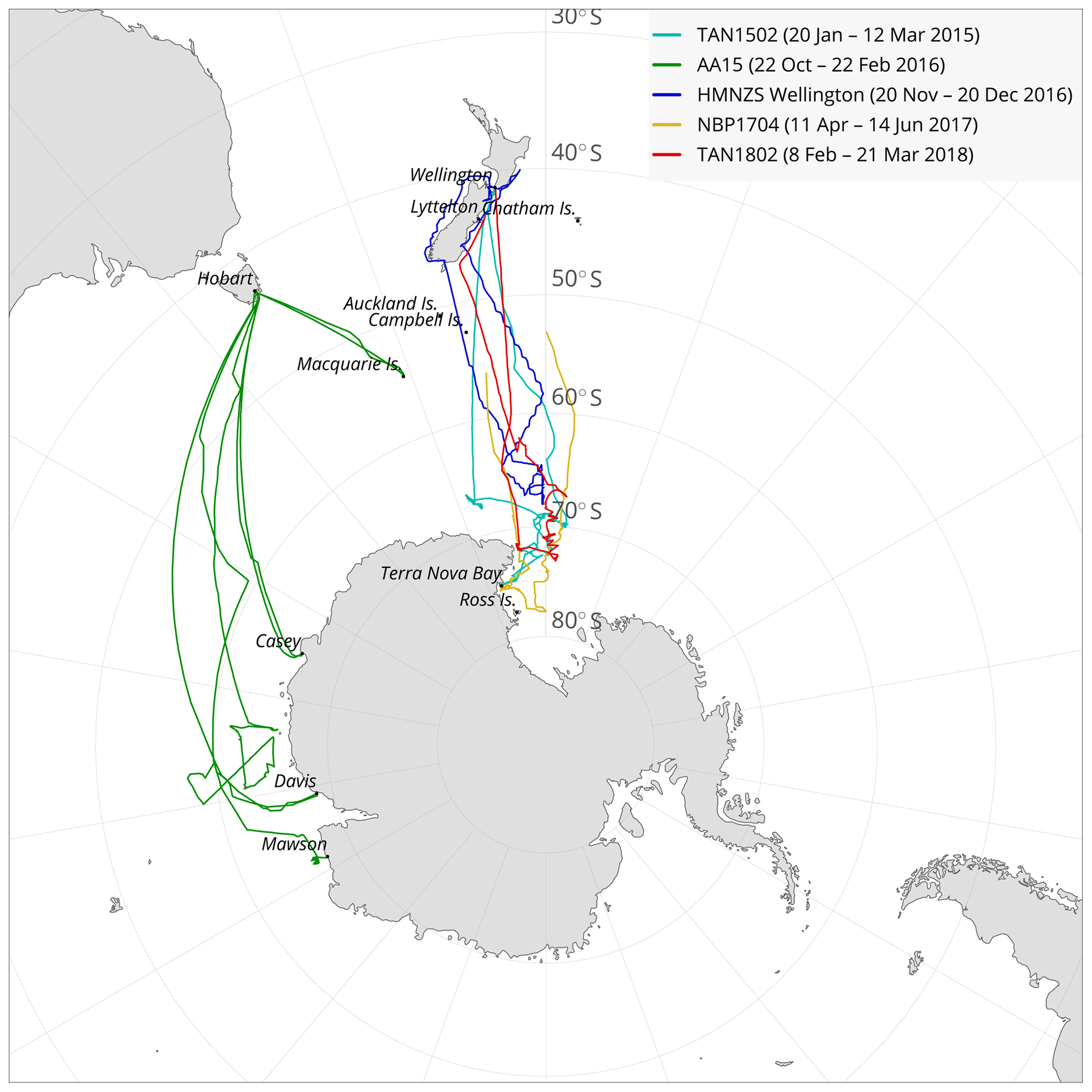
Figure 1Map showing tracks of voyages used in this study. The ship observational dataset is comprised of five voyages between 2015 and 2018, spanning the months of November to June and latitudes between 40 and 78∘ S, of which data between 50 and 70∘ S are used in this study.
Table 2Table of deployments. The table cells indicate if data from a given instrument (row) was available from a voyage (column).

Together, these voyages cover latitudes between 41 and 78∘ S and the months of November to June inclusive. A total of 298 d of observations were collected. Geographically, the voyages mostly cover the Ross Sea sector of the SO, with only AA15 covering the Indian Ocean sector (Fig. 1). This sampling emphasises the Ross Sea sector over other parts of the SO, although the SO SW radiation bias is present at all longitudes in the SO (Sect. 5.1), affected by the atmospheric circulation (Jones and Simmonds, 1993; Sinclair, 1994, 1995; Simmonds and Keay, 2000; Simmonds et al., 2003; Simmonds, 2003; Hoskins and Hodges, 2005; Hodges et al., 2011). The voyage observations were performed using a range of instruments (described below). Table 2 details which instruments were deployed on each voyage.
The primary instruments were the Lufft CHM 15k and Vaisala CL51 ceilometers. A ceilometer is an instrument which typically uses a single-wavelength laser to emit pulses vertically into the atmosphere and measures subsequent backscatter resolved on a large number of vertical levels based on the timing of the retrieved signal (Emeis, 2010). Depending on the wavelength, the emitted signal interacts with cloud droplets, ice crystals and precipitation by Mie scattering, and to a lesser extent with aerosol and atmospheric gases by Rayleigh scattering (Bohren and Huffman, 1998). The signal is quickly attenuated in thick cloud and therefore it is normally not possible to observe mid- and high-level parts of such a cloud or a multi-layer cloud. The main derived quantity determined from the backscatter is CBH, but it is also possible to apply a cloud detection algorithm to determine cloud occurrence by height. The range-normalised signal is affected by noise, which increases with the square of range. A major source of noise is solar radiation, which causes a diurnal variation in noise levels (Kotthaus et al., 2016). Due to signal attenuation and noise, ceilometers cannot measure clouds obscured by a lower cloud and therefore cannot be used for 1 : 1 comparison with model clouds without using a lidar simulator, which accounts for this effect (Chepfer et al., 2008). The Lufft CHM 15k ceilometer operates in the near-infrared spectrum at 1064 nm, measuring lidar backscatter up to a maximum height of 15 km, producing 1024 regularly spaced bins (about 15 m resolution). The sampling rate of the instrument is 2 s. The Vaisala CL51 ceilometer operates in the near-infrared spectrum at 910 nm. The sampling rate of the instrument is 2 s and range is 7.7 km, producing 770 regularly spaced bins (10 m resolution).
Radiosonde observations were performed on the TAN1802 and NBP1704 voyages south of 60∘ S. Temperature, pressure, relative humidity and Global Navigation Satellite System (GNSS) coordinates (from which wind speed and direction are derived) were retrieved to altitudes of about 10–20 km, terminated by a loss of radio communication or balloon burst.
On the TAN1802 voyage we used iMet-1 ABx radiosondes, measuring pressure, air temperature, relative humidity and GNSS coordinates of the sonde (from which wind speed and direction are derived). The sondes were launched three times a day at about 08:00, 12:00 and 20:00 UTC on 100 g Kaymont weather balloons. They reached a typical altitude of 10–20 km and then terminated by balloon burst or loss of radio communication. We used 10 s resolution profiles generated by the vendor-supplied iMetOS-II control software for further processing.
Automatic weather station (AWS) data were available on the TAN1502, TAN1802 and NBP1704 voyages. These included variables such as air temperature, pressure, sea surface temperature, wind speed and wind direction. Voyage track coordinates were obtained from the ships' GNSS receivers.
2.2 HadGEM3
HadGEM3 (Walters et al., 2019) is a general circulation model developed by the UK Met Office and the Unified Model Partnership. It can be used in a “nudging” (Telford et al., 2008) mode, in which winds and potential temperature are relaxed towards the ERA-Interim reanalysis (Dee et al., 2011). The Met Office Global Atmosphere 7.1 (GA7.1) is the atmospheric component of HadGEM3 (Walters et al., 2019), based on the Unified Model (UM) version 11.0.
The model runs used the HadISST sea surface temperature dataset (Rayner et al., 2003) as lateral boundary conditions. The nudged simulations represent atmospheric dynamics as determined by observations. The model was run on a (longitude × latitude) “N96” resolution grid, which corresponds to a horizontal resolution of about 100 km × 140 km at 60∘ S and 85 vertical levels. The model output fields were sampled every 6 h (instantaneous) and daily (mean). In our analysis we used a nudged run of GA7.1 (“GA7.1N”) between the years 2015 and 2018, corresponding to the ship observations.
2.3 MERRA-2
Modern-Era Retrospective analysis for Research and Applications (MERRA-2) is a reanalysis provided by the NASA Global Modelling and Assimilation Office (Gelaro et al., 2017). The reanalysis was chosen for its contrasting results of TOA outgoing SW radiation bias in the SO compared to GA7.1. As shown later (Fig. 3), its bias is positive rather than negative, when CERES is used as a reference.
We used the following products (Bosilovich et al., 2015):
-
1-hourly average Radiation Diagnostics (product “M2T1NXRAD.5.12.4”),
-
3-hourly instantaneous Assimilated Meteorological Fields (product “M2I3NVASM.5.12.4”),
-
1-hourly instantaneous Single-Level Diagnostics (product “M2I1NXASM.5.12.4”),
-
3-hourly average Assimilated Meteorological Fields (product “M2T3NVASM.5.12.4”),
-
1-hourly average Single-Level Diagnostics (product “M2T1NXSLV.5.12.4”).
We used the “Radiation Diagnostics” in TOA outgoing SW radiation evaluation (Sect. 5.1), the instantaneous “Assimilate Meteorological Fields” and “Single-Level Diagnostics” products to generate simulated ceilometer profiles and pseudo-radiosonde profiles (Sect. 5.2 and 5.3), and the average “Assimilate Meteorological Fields” and “Single-Level Diagnostics” to generate zonal plane plots of thermodynamic and cloud fields (Sect. 5.4). The four-dimensional MERRA-2 fields were provided on pressure and model levels. For our analysis we chose to use the model-level products (72 levels) due to their higher vertical resolution compared to pressure-level products. The analysed time period of MERRA-2 data was 2015–2018.
2.4 CERES
The Clouds and the Earth's Radiant Energy System (CERES) is a set of low Earth orbit (LEO) satellite instruments and a dataset of SW and longwave (LW) radiation observations (Loeb et al., 2018; Doelling et al., 2016). The CERES instruments (called FM1 to FM6) provide a continuous record of observations since the first deployment on the Tropical Rainfall Measuring Mission (TRMM) satellite in 1997 (Simpson et al., 1996) and have been flown on Terra, Aqua (Parkinson, 2003), the Suomi NPOESS Preparatory Project (Suomi NPP) and Joint Polar Satellite System-1 (JPSS-1) (Goldberg et al., 2013) satellites since. Currently CERES is considered the best available global Earth radiation datasets and is often used as the primary dataset for GCM tuning and validation (Schmidt et al., 2017; Hourdin et al., 2017). We used the following CERES products in our analysis:
-
CERES SYN1deg-Day edition 4A (configuration code 406406 and 407406) product of daily average radiation (“CERES SYN”),
-
CERES EBAF-TOA edition 4.1 (CERES_EBAF_Ed4.1) product of monthly energy-balanced average radiation (“CERES EBAF”).
Due to the sun-synchronous orbits of the LEO satellite platforms, the Flight Model (FM) instruments of CERES do not capture the full diurnal variation in radiation. The EBAF and SYN1deg products are adjusted for diurnal variation by using 1-hourly geostationary satellite observations between 60∘ S and 60∘ N, and use an algorithm to account for changing solar zenith angle and diurnal land heating. The CERES EBAF-TOA edition 4.1 product is a Level 3B product, which means it has been globally balanced by ocean heat measurements using the Argo network (Roemmich and Team, 2009).
2.5 NSIDC sea ice concentration
We used the Near-Real-Time Defense Meteorological Satellite Program (DMPS) Special Sensor Microwave Imager/Sounder (SSMIS) Daily Polar Gridded Sea Ice Concentrations, version 1 product (NSIDC-0081) (Maslanik and Stroeve, 1999) provided by the National Snow and Ice Data Center (NSIDC) to classify observations into those affected and unaffected by sea ice. The sea ice concentration product has a resolution of 25 km × 25 km. We used a cutoff value of 15 % of sea ice concentration for the binary classification of sea ice, in line with previous studies (Comiso and Nishio, 2008).
3.1 Lidar simulator
The CFMIP Observation Simulator Package (COSP) (Bodas-Salcedo et al., 2011), a set of instrument simulators developed by the Cloud Feedback Model Intercomparison Project (CFMIP), was extended with a surface lidar simulator and used to produce virtual lidar measurements from model fields (Kuma et al., 2020a). Resampling, noise reduction and cloud detection were performed on observational and (where applicable) model lidar data in a consistent way to reduce structural uncertainty (see Sect. 3.2). The schematic in Fig. 2 shows the processing pipeline utilised in this study.

Figure 2Schematic of the processing pipeline utilised in this study to produce lidar and radiosonde statistics from observations and model data.
COSP was originally developed as a satellite simulator package whose aim is to produce virtual satellite (and more recently ground-based) observations from atmospheric model fields in order to improve comparisons of model output with observations (Bodas-Salcedo et al., 2011). This approach is required because physical quantities derived from satellite observations generally do not directly correspond to model fields. COSP accounts for the limited view of the satellite instrument by calculating radiative transfer through the atmosphere, i.e. attenuation by hydrometeors and air molecules and backscattering. COSP comprises multiple instrument simulators, such as MODIS, ISCCP, MISR, CALIPSO and CloudSat. It has been used extensively by previous studies of model cloud, for example by Kay et al. (2012), Franklin et al. (2013), Klein et al. (2013), Williams and Bodas-Salcedo (2017), Jin et al. (2017), and Schuddeboom et al. (2018). COSP is planned to be used in the upcoming Coupled Model Intercomparison Project Phase 6 (CMIP6) (Webb et al., 2017).
For our analysis, we have developed a ground-based lidar simulator by modifying the COSP ACTSIM spaceborne lidar simulator (Chiriaco et al., 2006) (see the code and data availability section at the end of the document). This required reversing of the vertical layers, as the surface lidar looks from the surface up rather than down from space to the surface, and changing the radiation wavelength affecting Mie scattering by cloud droplets and Rayleigh scattering by air molecules. In this paper we present only a brief description of the surface lidar simulator, with a more complete description planned in an upcoming paper. The new simulator is made available as part of the Automatic Lidar and Ceilometer Framework (ALCF) at https://alcf-lidar.github.io (last access: 1 June 2020).
The recently introduced COSP version 2 (Swales et al., 2018) added support for a surface lidar simulator, although we believe our implementation, developed before COSPv2 was available, is more complete in the present context due to its treatment of Mie scattering at wavelengths other than 532 nm (the wavelength of the CALIPSO lidar). Previously, a surface lidar simulator based on COSP has been used by Chiriaco et al. (2018) and Bastin et al. (2018). A ground-based radar simulator in COSP has also recently been implemented (Zhang et al., 2018).
The surface lidar simulator takes model cloud liquid and ice mixing ratios, cloud fraction and thermodynamic profiles as the input, and calculates vertical profiles of attenuated backscatter. This can be done either by running the simulator “online” within the model code or “offline” on the model output. We used the offline approach in our analysis.
3.2 Lidar data processing
Lidar data in this study came from two different instruments: Lufft CHM 15k and Vaisala CL51 ceilometers and the lidar simulator. These instruments use different output formats, wavelengths, sampling rates and range bins, as previously noted. Backscatter and derived fields such as CBH are provided in the firmware-generated data products, but the backscatter is uncalibrated and the derived fields such as cloud detection are based on instrument-dependent algorithms. Therefore, we performed consistent subsampling, noise reduction and cloud detection on data from both instruments, and applied the same methods to the lidar simulator output. As part of the processing we developed a publicly available tool called cl2nc (“CL to NetCDF”) for converting the Vaisala CL51 ceilometer data format to NetCDF (see the code and data availability section at the end of the document).
3.2.1 Calibration
The backscatter profiles produced by the Lufft CHM 15k and Vaisala CL51 ceilometers are not calibrated to physical units, even though they are expressed in metres per steradian (m−1 sr−1). To calibrate these backscatter fields we used the method described by O'Connor et al. (2004). This method uses the lidar ratio (LR) to calculate a calibration factor based on a known value of the LR in fully scattering cloudy scenes (18.8±0.8 sr), such as thick stratocumulus clouds, which are common over the SO. We applied this technique by using visually identified scenes and choosing a calibration factor which achieves the known value. Due to the nature of the conditions (LR can be highly variable even in thick cloud scenes), the calibration is likely accurate to only about 50 % of the backscatter value. We do not expect this to have a serious impact on the accuracy of cloud detection completed in this study, largely because the predominantly low cloud tends to cause backscatter orders of magnitude greater than clear air and because of the very large differences in cloud occurrence between the observations and models.
3.2.2 Subsampling, noise removal and cloud detection
In order to simplify further processing and increase the signal-to-noise ratio, we subsampled the ceilometer observations at a sampling rate of 5 min by averaging multiple profiles, and vertically averaging on regularly spaced 50 m bins. We expect that in most cases cloud was almost constant on this timescale and vertical scale, and therefore we were not averaging together different cloud types or clear and cloudy profiles. At the same time as subsampling, we performed noise removal by estimating the noise distribution (mean and standard deviation) based on returns in the uppermost range bins (i.e. 300 samples over 5 min when sampling rate was 2 s) and subtracting the range-scaled noise mean from the backscatter. We then used the range-scaled noise standard deviation (σ) for cloud detection: a bin was considered cloudy if the calibrated backscatter minus 3σ exceeded m−1 sr−1. This threshold was chosen subjectively so that cloud was visually well separated from other features, such as boundary layer aerosol and noise on backscatter profile plots. The same threshold was used on both the observations and output from the COSP surface lidar simulator and thus should cause little bias.
3.2.3 Model lidar data processing
We used the same sampling rate (5 min) and model levels as range bins on the surface lidar simulator output. For each vertical profile we used model data at the same location as the ship and the same time relative to the start of the year. Model data were selected using nearest-neighbour interpolation. The model resolution is lower than the distance travelled by the ship in 5 min, therefore the same model data were used multiple times to generate consecutive profiles. However, we also used the SCOPS (Webb et al., 2001) subcolumn generator included in COSP to generate 10 random samples of cloud for each profile based on cloud fraction and the maximum–random cloud overlap assumption (Bodas-Salcedo, 2010). The lidar simulator processes each sample individually. The resulting cloud occurrence is calculated as the average of the 10 samples. The lidar simulator does not generate noise, and therefore we did not perform any noise removal on the simulated profiles, but we used the same threshold of m−1 sr−1 and vertical bins of 50 m for detecting cloud (as used on the observations). For the MERRA-2 cloud occurrence analysis, we applied the lidar simulator on the 3-hourly instantaneous Assimilated Meteorological Fields (M2I3NVASM.5.12.4) product.
Because our observational dataset does not span the entire geographical area of the SO and all months of the year, and the atmospheric conditions in the SO are geographically variable, we subset the datasets into a number of geographical regions (by latitude) and time periods (by season). The geographical regions investigated are 50–75∘ S by 5∘ of latitude, and the temporal periods investigated are austral summer of December, January, February (DJF) and autumn months of March, April, May (MAM).
We do not use data from 70 to 75 and 50 to 55∘ S in all parts of the analysis. The data from 70 to 75∘ S are likely affected by circulation induced by land near the Ross Sea (Coggins et al., 2014) and therefore may not be representative of the SO in general. This decision builds on the analysis detailed in Jolly et al. (2018) which shows a significant gradient in cloud properties between the Ross Ice Shelf and the Ross Sea and strong influences associated with synoptic conditions. The data from 50 to 55∘ S were relatively sparse (the ships spent relatively little time passing through these latitudes). Radiosonde observations were only available south of 60∘ S.
There is likely temporal variability present within the DJF and MAM time periods, but we decided to limit the number of temporal subsets to maintain a reasonable quantity of observations in each subset. The magnitude of the SO TOA outgoing SW radiation bias is primarily modulated by incoming solar radiation, which is the highest in DJF. The voyages do not uniformly cover all geographical regions or time periods, with the largest number of observations in the Ross Sea sector south of New Zealand (TAN1802, TAN1502, HMNZSW16 and NBP1704), followed by the Indian Ocean sector south of Western Australia (AA15). Temporally, the voyage observations mostly cover summer to autumn months of the year.
5.1 Shortwave radiation balance
Figure 3 shows TOA outgoing SW radiation in CERES, GA7.1 and MERRA-2. We present this panel plot in order to evaluate how well GA7.1N and MERRA-2 are performing in terms of SW radiation bias in the SO relative to CERES. This analysis assumes that CERES is a good observational reference, although it is affected by errors of lower order of magnitude (2.5 W m−2 “regional monthly uncertainty”; Loeb et al., 2018, Sect. 4a.). The plots reveal a relatively zonally symmetric pattern of negative and positive bias on the annual (Fig. 3b, c) and seasonal (Fig. 3e, f, h, i) timescales. GA7.1N shows predominantly negative bias, while MERRA-2 shows predominantly positive bias. The annual average is dominated by the bias in DJF due to the relatively strong incoming solar radiation in DJF. The bias displays very similar geographical pattern on the annual scale, DJF and MAM. The bias is much lower in MAM compared to DJF due to lower incoming solar radiation.
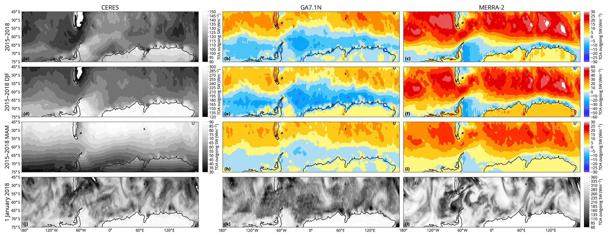
Figure 3Geographical distribution of the TOA outgoing SW radiation in CERES, GA7.1N and MERRA-2. The plots show global all-sky SW radiation as annual (2015–2018; a–c), seasonal (2015–2018 DJF, MAM; d–i) and daily (1 January 2018; j–l) mean. The blue–red colour map shows bias relative to CERES (b, c, e, f, h, i), while the grayscale colour map shows absolute values (a, d, g, j, k, l).
We chose 1 January 2018 as a representative day in DJF to show the daily scale. On the daily scale (Fig. 3j, k, l), the patterns are closely linked to synoptic features. The region on the eastern side of the Antarctic Peninsula shows the greatest negative bias in the models. The relatively zonally symmetric annual and seasonal means suggest that there is not a significant need for subsetting by longitude and that latitude averages can be very useful in identifying the key features of the SW radiation biases. The daily synoptic features are generally well correlated between CERES and the models, which is expected in nudged model runs and reanalyses. MERRA-2 has greater TOA outgoing SW radiation than GA7.1N on all three time periods presented here. Considering that cloud is the dominant factor affecting SW radiation in the SO, this can only be associated with either cloud cover that is too high or cloud albedo that is too high. GA7.1N reflects too little SW radiation south of 60∘ S and too much radiation north of 60∘ S (Fig. 3b, e, h). MERRA-2 reflects too much SW radiation in most of the SO, except for coastal regions of Antarctica (approx. 65–70∘ S) and the eastern side of the Antarctic Peninsula. The opposite sign of SW radiation bias in GA7.1N compared to MERRA-2 suggests that contrasting the two models could be useful for uncovering the cause of the bias.
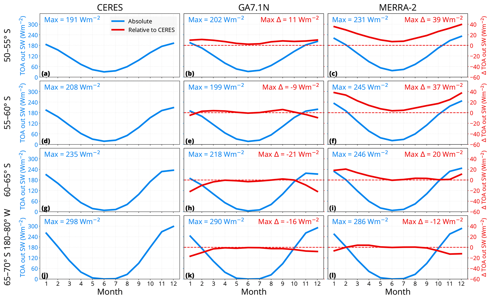
Figure 4Zonal means of the TOA outgoing SW radiation in CERES, GA7.1N and MERRA-2 during the years 2015–2018 in 5∘ latitude bands between 50 and 70∘ S. The plots show monthly zonal mean TOA outgoing SW radiation (blue) and its difference relative to CERES (red) as a function of month. Also shown are the maxima (“max”) and the difference from CERES (“max Δ”).
Figure 4 shows line plots of zonal mean reflected SW radiation and bias relative to CERES by month in multiple latitude bands between 50 and 70∘ S, with the southernmost band 65–70∘ S limited to 180–80∘W to avoid covering land areas in Antarctica. The annual cycle follows the expected seasonal pattern modulated by varying incoming solar radiation with maxima of reflected radiation in December and maxima of bias in December and January. The Antarctic sea ice extent, at its minimum in February and peaking in September, is also likely a secondary modulating factor of the TOA outgoing SW radiation at higher latitudes. The models represent the seasonal pattern well but differ substantially during the periods of peak incoming solar radiation. The GA7.1N model (Fig. 4b, e, h, k) exhibits bias ranging from −21 to +11 W m−2. The bias is positive north of 55∘ S and negative south of this latitude, with the greatest absolute bias between 60 and 65∘ S. MERRA-2 displays a clearly different bias from GA7.1N, ranging from −12 to 39 W m−2 (Fig. 4c, f, i, l). The peak SW bias in MERRA-2 is positive for latitudes north of 65∘ S and negative south of this latitude. The absolute bias in MERRA-2 is much larger than in GA7.1N north of 60∘ S and similar to GA7.1N south of this latitude. Therefore, the MERRA-2 results are valuable for contrasting with GA7.1. The strong latitudinal variation in the TOA outgoing SW radiation bias is important to take into consideration. Previous studies of SO clouds often did not discern different latitudes.

Figure 5Scatter plot of SW radiation bias in (a) GA7.1N and (b) MERRA-2 grid cells between 55 and 70∘ S in January 2018. Each point represents a daily average of SW radiation bias as a function of near-surface air temperature and near-surface relative humidity. The bias is expressed as a percentage of the incoming solar radiation in the grid cell. The points are a random sample of 100 000 points.
Figure 5 shows a scatter plot of the TOA outgoing SW radiation bias in GA7.1N and MERRA-2 as a function of near-surface air temperature and relative humidity between 55 and 70∘ S in January 2018. The bias is predominantly negative in GA7.1N and positive MERRA-2. There is a strong cluster of negative bias at temperature around 0 ∘C in GA7.1N and −2 ∘C in MERRA-2 and a cluster of positive bias at higher temperatures. This is consistent with the latitudinal dependence of bias in both models shown above.
5.2 Cloud occurrence in model and observations
To understand how clouds contribute to the SW bias, we examine cloud cover and cloud occurrence as a function of height in the models and observations. Figure 6 shows cloud occurrence profiles derived from ceilometer observations on different voyages and GA7.1N and MERRA-2 model output derived via the COSP surface lidar simulator, in subsets by latitude and season. Most notably, the observed cloud cover is consistently very high in the observations (80 %–100 %) for all periods and latitude bands examined and greater than 90 % in most of the subsets. This finding differs substantially from the modelled cloud cover derived via the surface lidar simulator, which ranges between 69 % and 100 % in GA7.1N, and is about 4 %–9 % lower than observations across the subsets. The cloud cover in MERRA-2 is also lower than observed and much lower than in GA7.1N, spanning 51 %–95 %. Only in four subsets is the cloud cover greater in GA7.1N than observed, and only in one subset is the cloud cover greater in MERRA-2 than observed (out of 21 subsets). Our analysis therefore shows that cloud cover is underestimated in both GA7.1N and MERRA-2 in the evaluated geographical regions and seasons.
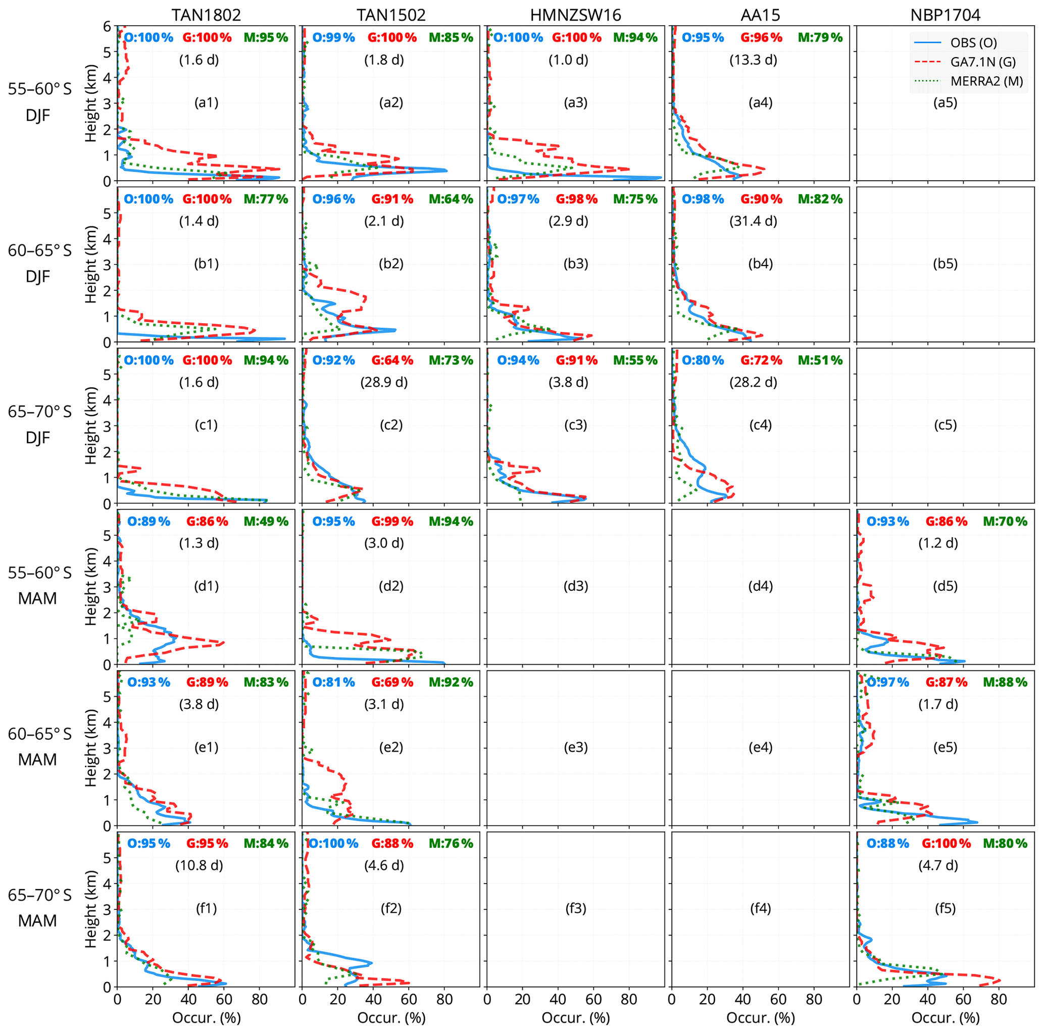
Figure 6Cloud occurrence frequency as a function of height derived from ceilometer observations (OBS) and model fields (GA7.1N and MERRA-2). The observational and model data were subsetted by latitude and season (DJF, MAM) along the voyage track. The numbers at the top of each panel show total (vertically integrated) cloud cover and the number of days the ship spent passing through the spatio-temporal subset. The height in the plots is limited to 6 km. There was no significant amount of cloud detected above this level.
Examination of the vertical distributions in Fig. 6 shows that observations have a strong predominance of cloud below 2 km and peaking below 500 m in most subsets, including a substantial amount of surface-level fog in some subsets. In contrast, GA7.1N and MERRA-2 simulate clouds at a higher altitude, peaking at about 500 m and generally the peak is higher than in observed clouds. Especially, clouds below 500 m and fog appear to be lacking in the models.
The subsets in Fig. 6 are derived from uneven length of ship observations (1.0–28.9 d) due to the limited availability of data. The longer subsets (Fig. 6a4, b4, c2, c4, f1) appear marginally more consistent between the models and observations in terms of the cloud occurrence profile, but the cloud cover is still markedly underestimated.
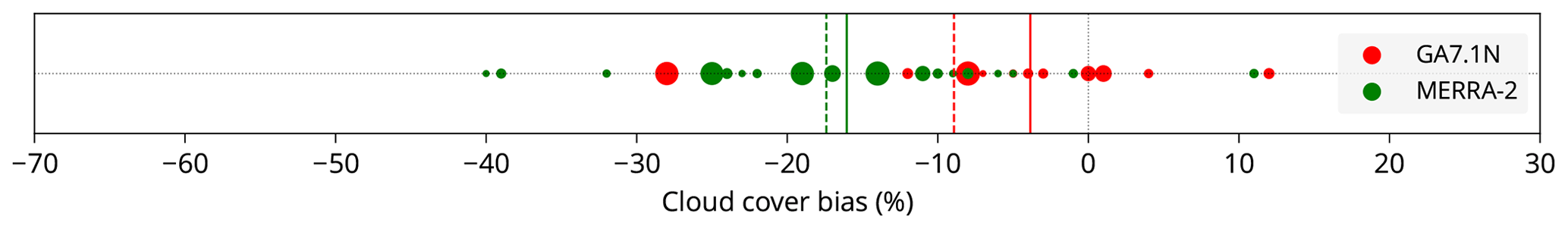
Figure 7Cloud cover bias in models relative to observations. The points represent subsets as in Fig. 6. The size of the circles is proportional to the number of days of observations in the subset. The solid lines are averages, and dashed lines are averages weighted by the number of days the ship spent passing through the spatio-temporal subset.
Figure 7 shows the model subsets of Fig. 6 as points by their cloud cover bias relative to observations. It can be seen that GA7.1N underestimates cloud cover by about 4 % and MERRA-2 by 16 % when non-weighted averages are considered, and by 9 % (GA7.1N) and 18 % (MERRA-2) when weighted averages are considered.
Due to the nature of the lidar measurements, middle to high clouds may be obscured by low clouds, as the laser signal is quickly attenuated by thick cloud. Therefore, the lack of clouds above 2 km in the plots does not imply that no clouds are present. The lidar simulator, however, ensures unbiased 1 : 1 comparison with observations by accounting for the signal attenuation.
The results demonstrate the value of surface cloud measurements in the SO relative to satellite measurements such as CloudSat and CALIPSO, which would likely provide a biased sample of these clouds because of “ground clutter” and obscuration by higher-level clouds, respectively (Alexander and Protat, 2018).
5.3 Radiosonde observations
We use radiosonde measurements performed on TAN1802 and NBP1704 to evaluate boundary layer properties and correlate them with clouds observed by a ceilometer. We compare the observations with “pseudo-radiosonde” profiles extracted from model fields at the same location and time. The location is based on the GNSS coordinates of the ship at the time of the balloon launch (the balloon trajectory length was generally not long enough to span multiple model grid cells in the lower troposphere).
We define a new quantity “SST lifting level” (SLL) derived from SST and boundary layer atmospheric potential temperature, defined as the level to which an air parcel with the same temperature as SST, rising from the sea surface, would rise adiabatically by buoyancy. That is, it is the level closest to the surface at which potential temperature is equal to SST, provided the air parcel is permitted to rise to this level by buoyancy (otherwise the air parcel does not rise and SLL is 0 m). This quantity is applicable in sea-ice-free conditions in the SO, when cold Antarctic air is warmed by the open sea surface and is lifted by buoyancy until it reaches a limit imposed by the atmospheric stability of the atmosphere. Alongside the lifting condensation level (LCL), we found SLL to be a useful quantity for evaluation of CBH. The authors are not aware of any previous use of SLL, but this definition is supported by observations (see below).
Apart from SLL and LCL, we also use the lower tropospheric stability (LTS) (Klein and Hartmann, 1993). LTS is defined as the difference between potential temperature at 700 hPa and sea level pressure (Klein and Hartmann, 1993). It has been used in multiple previous studies (Williams et al., 2006; Franklin et al., 2013; Williams et al., 2013; Naud et al., 2014).
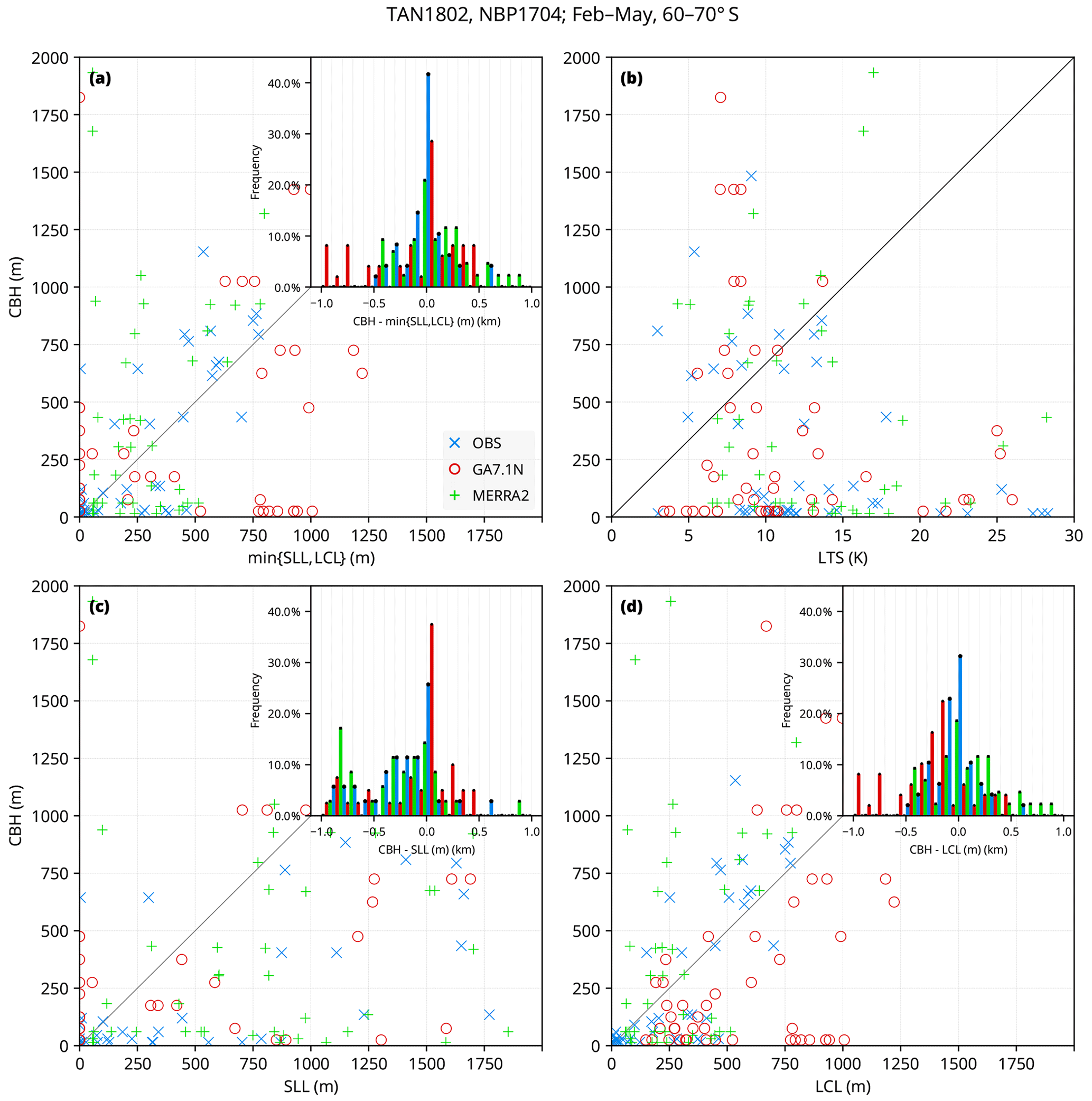
Figure 8Scatter plots of radiosonde measurements on the TAN1802 and NBP1704 voyages between February and May and 60 and 70∘ S latitude. Corresponding profiles from GA7.1N and MERRA-2 are selected, i.e. having the same geographical coordinates and the same time of the year. Each point on the scatter plots represents a radiosonde profile. The plots compare three datasets: observations (OBS), GA7.1N and MERRA-2. The radiosonde observations are matched with ceilometer (OBS) and COSP-based CBH (GA7.1N and MERRA-2). Panel (a) shows the points as a function of min{SLL, LCL} and CBH. The inset histogram shows distribution of the difference of CBH and min{SLL, LCL} in bins of 100 m, where each bin contains three bars for the three datasets. Panels (b), (c) and (d) show the points as a function of LTS, SLL and LCL, respectively.
Figure 8 shows the observed and modelled relationship between CBH and the minimum of SLL and LCL (“min{SLL,LCL}”), LTS, SLL and LCL. A large fraction of the observed points (OBS) in Fig. 8a lie close to the origin (40 % in the first 100 m in observations vs. 26 % and 17 % in GA7.1N and MERRA-2, respectively), which suggests that near zero min{SLL,LCL} is a good indicator of fog or very low cloud, a relationship not well represented in the models. The remaining observed points show a close equivalence between min{SLL,LCL} and CBH, while the models do not represent this equivalence well. The histogram in Fig. 8a reveals that about 42 % of observed profiles have CBH within 100 m of min{SLL,LCL}, while only about 28 % of GA7.1N and 21 % of MERRA-2 profiles do.
Using SLL or LCL as a predictor for CBH individually resulted in a weaker relationship than min{SLL,LCL}: 25 % and 31 % of OBS profiles have CBH within 100 m of SLL and LCL, respectively (Fig. 8c, d). This suggests that min{SLL,LCL} is more strongly related to CBH than SLL or LCL individually. Figure 8b shows CBH as a function of LTS. LTS does not display a good predictive ability for CBH in this dataset, with the exception of very stable profiles (LTS >15 K), when observed CBH was below 250 m in all but one case.
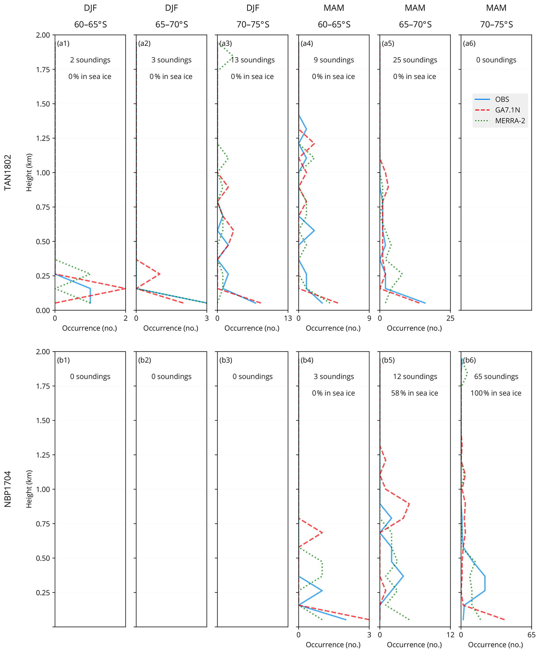
Figure 9Histogram of min{SLL,LCL} derived from radiosonde observations (OBS) on TAN1802 and NBP1704, and the equivalent profiles in GA7.1N and MERRA-2. Shown are subsets by latitude between 60 and 75∘ S and seasons DJF and MAM. The numbers at the top of each panel indicate the number of profiles that make up the histogram and the percentage of sea ice cases determined from NSIDC satellite-derived sea ice concentration.
Figure 9 shows the distribution of min{SLL,LCL} derived from radiosonde observations and model fields. In observations, the quantity almost consistently peaks near the ground and reaches up to 1.5 km in ice-free cases (Fig. 9a1–a5, b4). GA7.1N represents this distribution relatively well. This is not the case with MERRA-2, which is less likely to peak near the ground (Fig. 9a3, a5, c4). The sea-ice cases (Fig. 9b5, b6) show markedly different observed distribution of the quantity, with peak at about 300 m. GA7.1N and MERRA-2 represent the distribution over sea ice relatively poorly.
5.4 Zonal plane comparison of GA7.1N and MERRA-2
In order to better understand the differences in the SW radiation bias between GA7.1N and MERRA-2, we inspect zonal plane plots of cloud occurrence and thermodynamic fields of the models in DJF 2017/18 and 1 January 2018 (Fig. 10). The figure shows seasonal and daily average cloud liquid and ice mixing ratio contours plotted over two different backgrounds: potential temperature and relative humidity (RH). The daily average plots (Fig. 10c, d) show a very pronounced difference between the cloud liquid amount between the two models, with MERRA-2 simulating a much greater amount of cloud liquid. In contrast, GA7.1N simulates cloud with ice, which are nearly absent in MERRA-2 at the chosen contour levels. The liquid content is generally concentrated near SLL in MERRA-2 but much less so in GA7.1N, where SLL is often at 0 m. The cloud ice in GA7.1N generally has significantly greater vertical extent than the cloud liquid. These differences are also present on the seasonal scale (Fig. 10a, b). The difference in potential temperature between the models is relatively small. GA7.1N, however, shows a slightly higher potential temperature. The RH field is very different between GA7.1N and MERRA-2, with MERRA-2 simulating higher RH by about 10 %.

Figure 10Zonal plane plot of cloud liquid and ice mixing ratios in GA7.1N and MERRA-2 at 60∘ S. The cloud liquid and ice mixing ratios are plotted as contours on top of the potential temperature fields (a–d) and relative humidity fields (e–h). SLL is indicated by a white line. Panels (a), (b), (e) and (f) show a seasonal average in DJF 2017/2018, and panels (c), (d), (g) and (h) show a daily average on 1 January 2018. Panels (i) and (j) show the column-integrated values of cloud liquid and ice water as a function of longitude corresponding to the plots above. All liquid shown in the plots is supercooled (air temperature is less than 0 ∘C everywhere).
Perhaps most interestingly, the vertically integrated liquid and ice content (Fig. 10i, j) is very different between the models. Both models simulate almost the same liquid + ice total, but the phase composition of cloud in GA7.1N is majority ice, while in MERRA-2 it is almost entirely liquid.
The TOA outgoing SW radiation assessment shows that the models exhibit monthly average biases of up to 39 W m−2 (MERRA-2, 50–55∘ S in December), and that these biases have a significant latitudinal dependency, with the opposite sign of bias between different latitude bands. In GA7.1N the bias is predominantly negative, while in MERRA-2 the bias is predominantly positive. A similar pattern of bias is present in both models. The bias is positive north of 55∘ S (65∘ S) in GA7.1N (MERRA-2) and negative south of this latitude. This finding is consistent with Schuddeboom et al. (2019), who observed opposite sign of SW cloud radiative effect south and north of 55∘ S in GA7.1.
A very similar geographical pattern of bias is present in DJF and MAM, suggesting that similar cloud biases are present in both seasons. This is also supported by Fig. 6, which does not display a significant difference in observed cloud occurrence and bias in the models between DJF and MAM. Consistent with the maximum of incoming solar radiation, December and January were found to be the months with the greatest absolute bias in the models. Therefore, fixing the representation of clouds in the SO in these months is relatively more important than in other months.
Figure 5 suggests that the bias correlates not only with latitude but also with near-surface air temperature. The negative bias is strongly clustered around 0 ∘C in GA7.1N and −2 ∘C in MERRA-2, and positive bias is predominantly correlated with higher temperature.
The ship-based lidar cloud occurrence revealed close to 100 % cloud cover in multiple subsets. Subsetting allowed us to identify whether the cloud cover is substantially different by latitude and season and also sample independent weather situations (it is expected that cloud occurrence profiles are highly correlated over several days due to persistence of synoptic situations). The subsets show a relatively consistent cloud occurrence profile peaking below 500 m and almost zero above 2 km (possibly also due to obscuration of lidar signal by lower clouds). The models generally do not reproduce this profile well. Apart from underestimating the total cloud cover, the peak of cloud occurrence in the models is higher than observed. Improving the cloud profile representation in the models is likely key for improving the SW radiation bias.
The effect of clouds on SW radiation is the product of cloud cover (the fraction of the sky containing clouds) and cloud albedo (the fraction of SW radiation reflected by the clouds). With our ship-based lidar observations we measured cloud cover (total, and cloud cover as a function of height), while we did not measure cloud albedo. The cloud cover was almost consistently underestimated in both GA7.1N and MERRA-2 across all latitudes. At the same time, the satellite observations show that MERRA-2 reflects too much all-sky SW radiation. Therefore, the cloud albedo in MERRA-2 must be too high in order to cause too much all-sky SW radiation reflection despite the lack of cloud cover. This effect is visible on the daily scale in Fig. 3j–l, where the individual clouds in MERRA-2 appear significantly brighter than on satellite observations.
Remarkably, the observed cloud occurrence profiles appear to be similar between the DJF and MAM seasons and latitude bands between 55 and 70∘ S (Fig. 6): if we focus on the subsets with more than 10 d (Fig. 6a4, b4, c2, c4, f1), i.e. not heavily skewed toward a single weather situation, we find that they are all characterised by a peak below 500 m of 25 %–60 % and falling to near-zero above 2–3 km, sometimes with a minor secondary peak between 1 and 2 km. The simulated profiles show a slightly higher altitude of the primary peak between 0 and 1 km, underestimated in MERRA-2 by up about two-thirds and falling to near-zero between 2 and 3 km without any substantial secondary peak. The total cloud fraction appears to be more strongly underestimated at high latitudes in GA7.1N in DJF, by 8 %–28 % (Fig. 6c2, c4) vs. 8 % (Fig. 6b4). This is an important consideration in connection with the SW radiation bias, which shows a strong latitudinal gradient of the TOA outgoing SW radiation bias in the models (Figs. 3, 4). Based on the presented results, a plausible explanation for the SW radiation bias could be overestimation of cloud albedo north of about 55∘ S (65∘ S) in GA7.1N (MERRA-2) causing positive TOA outgoing SW radiation bias north of this latitude and underestimation of cloud cover over the whole SO causing negative TOA outgoing SW radiation bias south of this latitude.
In the ship observations we found a notable correspondence between CBH, SLL and LCL. Boundary layer thermodynamics, which determine the lifting levels, are a plausible driver of cloud formation in the absence of other forcing. We examined SLL in models and radiosonde observations and found differences which are likely too small to explain the cloud occurrence differences between the models and ceilometer observations. Bodas-Salcedo et al. (2012), in their analysis of an earlier version of the GA model (GA3.0) using cyclone composites also noted that biases in thermodynamics are not likely to explain the SW radiation bias but may still play a significant role. The presence of positive TOA outgoing SW radiation bias in the SO between 50 and 55∘ S in GA7.1, which contrasts with the negative bias south of the latitude, is important because it places a limit on the applicability of other studies, which used SO observational data from regions north of 55∘ S (Lang et al., 2018).
In Sect. 5.3 we show that min{SLL,LCL} has a stronger equivalence to CBH than SLL, LCL individually or LTS. This relationship becomes quite notable when examining the individual voyage radiosonde profiles (not presented here). We hypothesise that the theoretical reason for this relationship is the following. When SLL is higher than LCL, an air parcel warmed by the sea surface to temperature close to SST rises by buoyancy past LCL to a level with the equivalent potential temperature. The water vapour starts to condensate at LCL (assuming enough cloud condensation nuclei are present at 100 % saturation), forming cloud with CBH equal to LCL. If SLL is lower than LCL, the air parcel rises to the level of equivalent potential temperature, where air lifted from the sea surface eventually accumulates, potentially forming cloud if enough moisture is transported from the sea surface. The models do not represent the observed relationship well and improving this relationship may be one way of improving the cloud simulation.
Considering the strong observed relationship between min{SLL,LCL} and CBH (CBH tends to occur at the same level as min{SLL,LCL}), we evaluated the distribution of min{SLL,LCL} in the models in comparison with radiosonde observations (Fig. 9). We found that GA7.1N represents this distribution relatively well in sea-ice-free cases, while MERRA-2 underestimates cases when min{SLL,LCL} was near the surface. This may be the reason for the underestimation of very low cloud and fog in this model identified in the comparison with lidar observations. Therefore, improving the distribution of the quantity in MERRA-2 may lead to improvement of low cloud simulation.
It is interesting to contrast our results with previous studies which used cyclone compositing for the TOA SW radiation bias evaluation in GCMs. We cannot make substantial conclusions from our results on how much of the model bias is attributable to cyclones. It appears, however, that the cloud cover and cloud liquid and ice mixing ratio bias in GA7.1N is systematic rather than isolated to cyclonic activities due to its relative consistency across spatio-temporal subsets in the high-latitude SO. This does not rule out even greater biases related to cyclonic sectors. Specifically, Bodas-Salcedo et al. (2014) evaluated a large set of models, including HadGEM2-A, a predecessor model to HadGEM3, likely affected by similar biases and found that about 80 % of grid cells south of 55∘ S could be classified as affected by a cyclone, and that these grid cells were responsible for the majority of the total SW radiation bias. Moreover, their cyclone compositing showed that the bias in HadGEM2-A was largely negative in the cold quadrants, and near zero in the warm quadrants. Their results also indicate a strong contrast in SW bias south and north of 55∘ S, similar to the result we found in GA7.1N. We think these results can be reconciled with our study by assuming that the model has a particular difficulty in representing cloud in situations when near-surface air temperature is lower than the SST. In these regions the heat flux from the ocean to the atmosphere is positive, which in the austral summer predominantly occur south of 55∘ S and in the cold sectors of cyclones. The cloud representation when near-surface air temperature is greater than SST is relatively accurate, this case occurring predominantly north of 55∘ S and in the warm sector of cyclones. As shown in Fig. 5, the negative TOA outgoing SW radiation bias in the models is clustered at zero and sub-zero temperatures. This suggests a possible explanation that sub-zero air mass advecting from Antarctica or from sea-ice-covered areas over warm water (cold-air outbreaks) could be inducing low cloud and fog and that this process is not well represented in the models (Bodas-Salcedo et al., 2012).
Previous studies have documented that supercooled liquid is often present in the SO cloud in summer months (Morrison et al., 2011; Huang et al., 2012; Chubb et al., 2013; Huang et al., 2016; Bodas-Salcedo et al., 2016; Jolly et al., 2018; Listowski et al., 2019). We cannot substantially add to these findings with our observations, although preliminary analysis of a polarising lidar Sigma Space MiniMPL profiles from the TAN1802 voyage suggests supercooled liquid was commonly present in the ubiquitous stratocumulus cloud. The side-by-side comparison of cloud liquid and ice mixing ratios on the zonal plane (Fig. 10) suggests that models can differ significantly in their representation of cloud phase, with GA7.1N simulating markedly less supercooled liquid than MERRA-2. This is the most likely the explanation for the overestimation of TOA outgoing SW radiation in MERRA-2, despite the underestimated cloud cover in this model. If cloud cover is increased in MERRA-2 to better match with the lidar observations, the cloud albedo would have to be lowered to obtain a reasonable match of TOA outgoing SW radiation with CERES.
The 2016–2018 voyages may have been affected by the unusually low sea ice extent (discussed below), which can have a significant effect on cloud (Frey et al., 2018; Taylor et al., 2015). The modulating effect of sea ice on cloud in the SO has previously been shown by Listowski et al. (2019) and there is an apparent difference in cloud between the Ross Sea and Ross Ice Shelf, as shown by Jolly et al. (2018), with cloud over the ice shelf having smaller cloud cover, a greater amount of altostratus cloud and a smaller amount of deep convective cloud. The sea ice and ice shelves block transport of heat and moisture to the atmosphere. Their low thermal conductivity and high albedo mean the surface can cool to very low temperature and thus have an effect on the radiation balance of the atmosphere. We did not focus on sea ice conditions, since one can expect the effect of cloud biases on the SW radiation bias over sea ice to be small – the ice surface is already highly reflective in the SW, and the presence of cloud has little impact on the grid cell SW reflectivity (the SW albedo of cloud is similar to sea ice, depending on the sea ice concentration).
Antarctic sea ice extent underwent a rapid decrease starting in the spring of 2016 after about a decade of slightly increasing extent (Turner et al., 2017; Stuecker et al., 2017; Doddridge and Marshall, 2017; Kusahara et al., 2018; Schlosser et al., 2018; Ludescher et al., 2018). The sea ice extent due to this decrease was found to be the lowest on observational record since 1979, and the Ross Sea was particularly affected by this anomaly. The unusually low sea ice extent likely affected atmospheric observations made on the voyages presented in this study, e.g. the TAN1802 voyage in February and March 2018 to the Ross Sea experienced no sea ice during the entire voyage. Because sea ice is an important factor influencing the atmospheric boundary layer stability and radiation balance, a significant secondary effect on cloud cover, cloud phase and opacity is expected. Sea ice is, however, not expected to be responsible for the SO SW radiation bias described here because the bias is present even when sea ice concentration is prescribed from satellite observations, as is the case in the nudged run GA7.1 and the MERRA-2 reanalysis. Given that few of the ship-based observations were collected before 2016, we cannot reliably estimate how the anomalous sea ice extent affected our results.
In our results we found that even when model atmospheric dynamics are prescribed based on past observations, the TOA outgoing SW radiation bias is large and cloud occurrence, especially of low cloud and fog, is underestimated. CBH is found to be strongly linked to the boundary layer thermodynamics, and this link does not seem to be well represented in GA7.1N and MERRA-2. We therefore expect that cloud and boundary layer parameterisations (as part of subgrid-scale processes in the models) are responsible for this bias. We have identified the parts of the GA7.1N model that are most likely to be responsible: the large-scale cloud scheme, the PC2 scheme (Wilson et al., 2008a, b) and the boundary layer scheme. A future study should focus on these schemes to identify the parts responsible for the bias. In particular, the model should improve simulation of very low cloud and fog and achieve a closer match between the lifting levels and CBH (Fig. 8a).
Table 3A table showing a “back-of-the-envelope” calculation of how the GA7.1N peak TOA outgoing SW radiation bias (Fig. 4) would change if the cloud cover were increased by 5 % (Fig. 7), assuming the cloud albedo does not change. The “corrected” TOA outgoing SW radiation is calculated by multiplying the original value by 1.05.
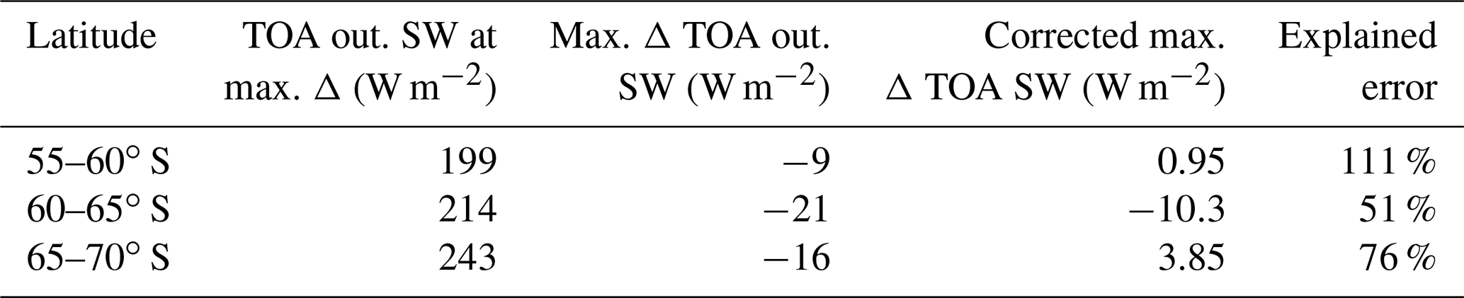
In Table 3 we present a simple calculation of how the GA7.1N peak TOA outgoing SW radiation bias would change if the cloud cover were increased by 5 % (as suggested by Fig. 7), assuming the cloud albedo does not change. This correction would explain 51 %–111 % of the bias depending on the latitude. The remaining part of the bias must be attributed to cloud albedo. One way this could be improved is by increasing the supercooled liquid fraction, or by increasing the total cloud water (liquid + ice) path. Therefore, our results suggest that in GA7.1N underestimation of cloud cover is responsible for the majority of the negative TOA outgoing SW radiation bias, relative to underestimation of cloud albedo.
We analysed 4 years of observational SO ship data, and contrasted them with a nudged run of the GA7.1 GCM and MERRA-2 reanalysis. We used satellite observations of the Earth radiation budget to assess the TOA outgoing SW radiation bias in the SO in the models. We examined the total cloud cover and vertical distribution of cloud as measured by ceilometers and simulated by a ceilometer simulator based on the model data. We also compared SO radiosonde observations from two voyages with pseudo-radiosonde profiles from the models in order to assess boundary layer stability and the correlation between cloud base and atmospheric lifting levels. We also compared model fields of cloud liquid and ice content, potential temperature and relative humidity in a zonal plane analysis across the SO to contrast cloud and thermodynamics simulated by GA7.1N and MERRA-2.
The SO SW radiation bias is significant in GA7.1N and MERRA-2 and tends to be positive in the northern parts of the SO and negative in the southern parts of the SO in both models. MERRA-2 shows greater absolute bias than GA7.1N. SO ship-based lidar and radiosonde observations are a valuable tool for model cloud evaluation, considering the amount of low cloud in this region which is likely poorly sampled by satellite instruments due to possible obscuration by higher overlapping cloud. The main findings of this study are that multi-year ship-based observations are as follows:
-
corroborating satellite-based evidence of underestimated cloud cover, with both GA7.1N and MERRA-2 underestimating cloud cover on average by about 4 %–9 % (GA7.1N) and 18 % (MERRA-2);
-
showing that low cloud below 2 km is almost continuous in the SO in summer months in sea-ice-free conditions and not well represented in the models;
-
indicating that boundary layer thermodynamics are a strong driver of cloud in the SO and that this relationship is not well represented in the models;
-
suggesting that subgrid-scale processes in situations when near-surface atmospheric temperature is lower or close to SST are responsible for the cloud misrepresentation.
Here, we introduced a new quantity (a thermodynamic level) called SST lifting level (SLL), which is the level of neutral buoyancy of an adiabatically lifted parcel with temperature equal to SST. The motivation for introducing this level was the frequently observed occurrence of cloud base at this height, together with LCL. We think that this is explained by the strongly thermodynamically driven cloud in the Southern Ocean boundary layer and is linked to the particular conditions of the summertime Southern Ocean: sub-zero temperatures of the near-surface atmosphere, which are destabilised by the relatively warmer (near-zero) sea surface.
Future studies of SO cloud representation in the GA model could focus on specific details of the model subgrid-scale cloud processes (such as the large-scale cloud, boundary layer and convection schemes), and how their tuning impacts cloud occurrence distributions compared to the ship observations. The stark difference between GA7.1N and MERRA-2 cloud liquid and ice content also remains to be explained, and could provide valuable insight for improving the SO SW radiation bias in the model and the reanalysis.
The original COSP version 1 simulator is open source and available publicly at https://github.com/CFMIP/COSPv1 (Bodas-Salcedo and Swales, 2018). The modified COSP version 1 simulator, including the ground-based lidar simulator used in this study is open source and available at https://alcf-lidar.github.io (Kuma et al., 2020b). The cl2nc software for converting Vaisala CL51 data to NetCDF is available at https://github.com/peterkuma/cl2nc (Kuma, 2020). The CERES EBAF and SYN1deg products are available publicly from the CERES website: https://doi.org/10.5067/TERRA-AQUA/CERES/EBAF-TOA_L3B004.1 (Doelling, 2019). The Near-Real-Time DMPS SSMIS Daily Polar Gridded Sea Ice Concentrations product is available publicly from the NSIDC website: https://doi.org/10.5067/U8C09DWVX9LM (Maslanik, 1999). The Hadley Centre Sea Ice and Sea Surface Temperature dataset (HadISST) is available publicly from the Met Office website: https://www.metoffice.gov.uk/hadobs/hadisst/ (Rayner et al., 2019). The MERRA-2 data are available publicly from the MERRA-2 website: https://gmao.gsfc.nasa.gov/reanalysis/MERRA-2/ (Gelaro et al., 2016). The ship-based observations dataset, as well as all processing code, is available on request from the authors.
PK participated in methodology development, voyage observations, data analysis, writing and reviewing of the manuscript. AJM participated in conceptualisation, funding acquisition, methodology development, voyage observations, data analysis, writing and reviewing of the manuscript. OM participated in model development, methodology development, data analysis, writing and reviewing of the manuscript. SPA, JJC, JH, SH, SG, MJH, SP, and GP participated in voyage observations and reviewing of the manuscript. VV and JW participated in model development and reviewing of the manuscript.
The authors declare that they have no conflict of interest.
We would like to thank the editor Patrick Chuang and two anonymous referees for reviewing the manuscript. We would like to thank everyone who participated in obtaining the Southern Ocean voyage observations, especially Kelly Schick and Peter Guest for performing ceilometer and radiosonde measurements on RV Nathaniel B. Palmer, the Royal New Zealand Navy for ceilometer and radar measurements on HMNZS Wellington, Alex Schuddeboom for deployment of instruments on RV Nathaniel B. Palmer; and the crews of the TAN1502 Aurora Australis V1–V3 2015/16 and HMNZS Wellington NBP1704 and TAN1802 voyages. Logistical and technical support for the ceilometer observations made aboard Aurora Australis during the summer of 2015/16 were provided as part of the Australian Antarctic Science project 4292. We acknowledge the Met Office for use of the MetUM and for providing the HadGEM3 model. We acknowledge NASA-GMAO and ECMWF for the MERRA-2 and ERA-Interim reanalyses, respectively. We acknowledge the software tools Python, R (R Core Team, 2018), NumPy (Oliphant, 2006), SciPy (Virtanen et al., 2020), Matplotlib (Hunter, 2007), Climate Data Operators (CDO) (Schulzweida, 2018) and parallel (Tange, 2011), all of which we used in our data analysis.
This research has been supported by the Deep South National Science Challenge Clouds and Aerosols project, New Zealand; the Australian Antarctic Science project (grant no. 4292); and the NeSI collaborator institutions and Ministry of Business, Innovation & Employment Research Infrastructure programme, New Zealand.
This paper was edited by Patrick Chuang and reviewed by two anonymous referees.
Alexander, S. and Protat, A.: Cloud properties observed from the surface and by satellite at the northern edge of the Southern Ocean, J. Geophys. Res.-Atmos., 123, 443–456, https://doi.org/10.1002/2017jd026552, 2018. a
Bastin, S., Chiriaco, M., and Drobinski, P.: Control of radiation and evaporation on temperature variability in a WRF regional climate simulation: comparison with colocated long term ground based observations near Paris, Clim. Dynam., 51, 985–1003, https://doi.org/10.1007/s00382-016-2974-1, 2018. a
Bodas-Salcedo, A.: COSP user's manual: Version 1.3.1, Met Office Hadley Centre, Exeter, UK, 2010. a
Bodas-Salcedo, A. and Swales, D.: CFMIP Observation Simulator Package, available at: https://github.com/CFMIP/COSPv1 (last access: 2 June 2020), 2018. a
Bodas-Salcedo, A., Webb, M., Bony, S., Chepfer, H., Dufresne, J.-L., Klein, S., Zhang, Y., Marchand, R., Haynes, J., Pincus, R., and John, V. O.: COSP: Satellite simulation software for model assessment, B. Am. Meteorol. Soc., 92, 1023–1043, https://doi.org/10.1175/2011bams2856.1, 2011. a, b
Bodas-Salcedo, A., Williams, K., Field, P., and Lock, A.: The surface downwelling solar radiation surplus over the Southern Ocean in the Met Office model: The role of midlatitude cyclone clouds, J. Climate, 25, 7467–7486, https://doi.org/10.1175/JCLI-D-11-00702.1, 2012. a, b, c, d
Bodas-Salcedo, A., Williams, K. D., Ringer, M. A., Beau, I., Cole, J. N., Dufresne, J.-L., Koshiro, T., Stevens, B., Wang, Z., and Yokohata, T.: Origins of the solar radiation biases over the Southern Ocean in CFMIP2 models, J. Climate, 27, 41–56, https://doi.org/10.1175/JCLI-D-13-00169.1, 2014. a, b, c, d
Bodas-Salcedo, A., Hill, P., Furtado, K., Williams, K., Field, P., Manners, J., Hyder, P., and Kato, S.: Large contribution of supercooled liquid clouds to the solar radiation budget of the Southern Ocean, J. Climate, 29, 4213–4228, https://doi.org/10.1175/jcli-d-15-0564.1, 2016. a, b, c, d
Bohren, C. F. and Huffman, D. R.: Absorption and scattering of light by small particles, John Wiley & Sons, Hoboken, NJ, USA, 1998. a
Bony, S., Stevens, B., Frierson, D. M., Jakob, C., Kageyama, M., Pincus, R., Shepherd, T. G., Sherwood, S. C., Siebesma, A. P., Sobel, A. H., Watanabe, M., and Webb, M. J.: Clouds, circulation and climate sensitivity, Nat. Geosci., 8, 261–268, https://doi.org/10.1038/ngeo2398, 2015. a
Bosilovich, M., Lucchesi, R., and Suarez, M.: MERRA-2: File specification, GMAO Office Note No. 9 (Version 1.1), Global Modeling and Assimilation Office, Greenbelt, MD, USA, available at: http://gmao.gsfc.nasa.gov/pubs/office_notes (last access: 2 June 2020), 2015. a
Boucher, O., Randall, D., Artaxo, P., Bretherton, C., Feingold, G., Forster, P., Kerminen, V.-M., Kondo, Y., Liao, H., Lohmann, U., Rasch, P., Satheesh, S., Sherwood, S., Stevens, B., and Zhang, X.: Clouds and aerosols, in: Climate change 2013: the physical science basis. Contribution of Working Group I to the Fifth Assessment Report of the Intergovernmental Panel on Climate Change, edited by: Stocker, T., Qin, D., Plattner, G.-K., Tignor, M., Allen, S., Boschung, J., Nauels, A., Xia, Y., Bex, V., and Midgley, P., Cambridge University Press, Cambridge, UK and New York, NY, USA,, 571–657, 2013. a
Ceppi, P., Hwang, Y.-T., Frierson, D. M., and Hartmann, D. L.: Southern Hemisphere jet latitude biases in CMIP5 models linked to shortwave cloud forcing, Geophys. Res. Lett., 39, L19708, https://doi.org/10.1029/2012GL053115, 2012. a
Chepfer, H., Bony, S., Winker, D., Chiriaco, M., Dufresne, J.-L., and Sèze, G.: Use of CALIPSO lidar observations to evaluate the cloudiness simulated by a climate model, Geophys. Res. Lett., 35, L15704, https://doi.org/10.1029/2008gl034207, 2008. a
Chiriaco, M., Vautard, R., Chepfer, H., Haeffelin, M., Dudhia, J., Wanherdrick, Y., Morille, Y., and Protat, A.: The ability of MM5 to simulate ice clouds: Systematic comparison between simulated and measured fluxes and lidar/radar profiles at the SIRTA atmospheric observatory, Mon. Weather Rev., 134, 897–918, https://doi.org/10.1175/MWR3102.1, 2006. a
Chiriaco, M., Dupont, J.-C., Bastin, S., Badosa, J., Lopez, J., Haeffelin, M., Chepfer, H., and Guzman, R.: ReOBS: a new approach to synthesize long-term multi-variable dataset and application to the SIRTA supersite, Earth Syst. Sci. Data, 10, 919–940, https://doi.org/10.5194/essd-10-919-2018, 2018. a
Chubb, T. H., Jensen, J. B., Siems, S. T., and Manton, M. J.: In situ observations of supercooled liquid clouds over the Southern Ocean during the HIAPER Pole-to-Pole Observation campaigns, Geophys. Res. Lett., 40, 5280–5285, https://doi.org/10.1002/grl.50986, 2013. a, b
Coggins, J. H., McDonald, A. J., and Jolly, B.: Synoptic climatology of the Ross Ice Shelf and Ross Sea region of Antarctica: k-means clustering and validation, Int. J. Climatol., 34, 2330–2348, https://doi.org/10.1002/joc.3842, 2014. a
Comiso, J. C. and Nishio, F.: Trends in the sea ice cover using enhanced and compatible AMSR-E, SSM/I, and SMMR data, J. Geophys. Res.-Oceans, 113, C02S07, https://doi.org/10.1029/2007JC004257, 2008. a
Dee, D. P., Uppala, S. M., Simmons, A., Berrisford, P., Poli, P., Kobayashi, S., Andrae, U., Balmaseda, M., Balsamo, G., Bauer, D. P., Bechtold, P., Beljaars, A. C. M., van de Berg, L., Bidlot, J., Bormann, N., Delsol, C., Dragani, R., Fuentes, M., Geer, A. J., Haimberger, L., Healy, S. B., Hersbach, H., Hólm, E. V., Isaksen, L., Kållberg, P., Köhler, M., Matricardi, M., McNally, A. P., Monge-Sanz, B. M., Morcrette, J.-J., Park, B.-K., Peubey, C., de Rosnay, P., Tavolato, C., Thépaut, J.-N., and Vitart, F.: The ERA-Interim reanalysis: Configuration and performance of the data assimilation system, Q J. Roy. Meteor. Soc., 137, 553–597, https://doi.org/10.1002/qj.828, 2011. a
Doelling, D.: CERES Energy Balanced and Filled (EBAF) TOA Monthly means data in netCDF Edition4.1, CERES, https://doi.org/10.5067/TERRA-AQUA/CERES/EBAF-TOA_L3B004.1, 2019. a
Doddridge, E. W. and Marshall, J.: Modulation of the seasonal cycle of Antarctic sea ice extent related to the Southern Annular Mode, Geophys. Res. Lett., 44, 9761–9768, https://doi.org/10.1002/2017gl074319, 2017. a
Doelling, D. R., Haney, C. O., Scarino, B. R., Gopalan, A., and Bhatt, R.: Improvements to the geostationary visible imager ray-matching calibration algorithm for CERES Edition 4, J. Atmos. Ocean. Tech., 33, 2679–2698, https://doi.org/10.1175/jtech-d-16-0113.1, 2016. a
Emeis, S.: Surface-based remote sensing of the atmospheric boundary layer, vol. 40, Springer Science & Business Media, https://doi.org/10.1007/978-90-481-9340-0, 2010. a
Flato, G., Marotzke, J., Abiodun, B., Braconnot, P., Chou, S. C., Collins, W., Cox, P., Driouech, F., Emori, S., Eyring, V., Forest, C., Gleckler, P., Guilyardi, E., Jakob, C., Kattsov, V., Reason, C., and Rummukainen, M.: Evaluation of climate models, in: Climate change 2013: the physical science basis. Contribution of Working Group I to the Fifth Assessment Report of the Intergovernmental Panel on Climate Change, Cambridge University Press, 741–866, https://doi.org/10.1017/CBO9781107415324.020, 2014. a
Franklin, C. N., Sun, Z., Bi, D., Dix, M., Yan, H., and Bodas-Salcedo, A.: Evaluation of clouds in ACCESS using the satellite simulator package COSP: Regime-sorted tropical cloud properties, J. Geophys. Res.-Atmos., 118, 6663–6679, https://doi.org/10.1002/jgrd.50496, 2013. a, b
Frey, W., Morrison, A., Kay, J., Guzman, R., and Chepfer, H.: The combined influence of observed Southern Ocean clouds and sea ice on top-of-atmosphere albedo, J. Geophys. Res.-Atmos., 123, 4461–4475, https://doi.org/10.1029/2018JD028505, 2018. a
Gelaro, R., McCarty, W., Suárez, M. J., Todling, R., Molod, A., Takacs, L., Randles, C. A., Darmenov, A., Bosilovich, M. G., Reichle, R., Wargan, K., Coy, L., Cullather, R., Draper, C., Akella, S., Buchard, V., Conaty, A., da Silva, A. M., Gu, W., Kim, G.-K., Koster, R., Lucchesi, R., Merkova, D., Nielsen, J. E., Partyka, G., Pawson, S., Putman, W., Rienecker, M., Schubert, S. D., Sienkiewicz, M., and Zhao, B.: Modern-Era Retrospective Analysis for Research and Applications, Version 2, available at: https://gmao.gsfc.nasa.gov/reanalysis/MERRA-2/ (last access: 2 June 2020), 2016. a
Gelaro, R., McCarty, W., Suárez, M. J., Todling, R., Molod, A., Takacs, L., Randles, C. A., Darmenov, A., Bosilovich, M. G., Reichle, R., Wargan, K., Coy, L., Cullather, R., Draper, C., Akella, S., Buchard, V., Conaty, A., da Silva, A. M., Gu, W., Kim, G.-K., Koster, R., Lucchesi, R., Merkova, D., Nielsen, J. E., Partyka, G., Pawson, S., Putman, W., Rienecker, M., Schubert, S. D., Sienkiewicz, M., and Zhao, B.: The modern-era retrospective analysis for research and applications, version 2 (MERRA-2), J. Climate, 30, 5419–5454, https://doi.org/10.1175/JCLI-D-16-0758.1, 2017. a
Goldberg, M. D., Kilcoyne, H., Cikanek, H., and Mehta, A.: Joint Polar Satellite System: The United States next generation civilian polar-orbiting environmental satellite system, J. Geophys. Res.-Atmos., 118, 13–463, https://doi.org/10.1002/2013jd020389, 2013. a
Hartery, S., Kuma, P., McGregor, J., Marriner, A., Sellegri, K., Saint-Macary, A., Law, C., von Hobem, M., Kremser, S., Lennartz, S., Archer, S., DeMott, P., Hill, T., Querel, R., Brailsford, G., Geddes, A., Parsons, S., McDonald, A., and Harvey, M.: Atmospheric Measurements During the Antarctic and Southern Ocean Marine Environment and Ecosystem Study (ASOMEES), in preparation, 2019. a
Haynes, J. M., Jakob, C., Rossow, W. B., Tselioudis, G., and Brown, J.: Major characteristics of Southern Ocean cloud regimes and their effects on the energy budget, J. Climate, 24, 5061–5080, https://doi.org/10.1175/2011jcli4052.1, 2011. a
Hodges, K. I., Lee, R. W., and Bengtsson, L.: A comparison of extratropical cyclones in recent reanalyses ERA-Interim, NASA MERRA, NCEP CFSR, and JRA-25, J. Climate, 24, 4888–4906, https://doi.org/10.1175/2011jcli4097.1, 2011. a
Hoskins, B. J. and Hodges, K. I.: A new perspective on Southern Hemisphere storm tracks, J. Climate, 18, 4108–4129, https://doi.org/10.1175/jcli3570.1, 2005. a
Hourdin, F., Mauritsen, T., Gettelman, A., Golaz, J.-C., Balaji, V., Duan, Q., Folini, D., Ji, D., Klocke, D., Qian, Y., Rauser, F., Rio, C., Tomassini, L., Watanabe, M., and Williamson, D.: The art and science of climate model tuning, B. Am. Meteorol. Soc., 98, 589–602, https://doi.org/10.1175/BAMS-D-15-00135.1, 2017. a
Huang, Y., Siems, S. T., Manton, M. J., Protat, A., and Delanoë, J.: A study on the low-altitude clouds over the Southern Ocean using the DARDAR-MASK, J. Geophys. Res.-Atmos., 117, D18204, https://doi.org/10.1029/2012JD017800, 2012. a, b
Huang, Y., Siems, S. T., Manton, M. J., Rosenfeld, D., Marchand, R., McFarquhar, G. M., and Protat, A.: What is the role of sea surface temperature in modulating cloud and precipitation properties over the Southern Ocean?, J. Climate, 29, 7453–7476, https://doi.org/10.1175/JCLI-D-15-0768.1, 2016. a, b
Hunter, J. D.: Matplotlib: A 2D graphics environment, Comput. Sci. Eng., 9, 90–95, https://doi.org/10.1109/MCSE.2007.55, 2007. a
Hwang, Y.-T. and Frierson, D. M.: Link between the double-Intertropical Convergence Zone problem and cloud biases over the Southern Ocean, P. Natl. Acad. Sci. USA, 110, 4935–4940, https://doi.org/10.1073/pnas.1213302110, 2013. a
Hyder, P., Edwards, J. M., Allan, R. P., Hewitt, H. T., Bracegirdle, T. J., Gregory, J. M., Wood, R. A., Meijers, A. J., Mulcahy, J., Field, P., Furtado, K., Bodas-Salcedo, A., Williams, K. D., Copsey, D., Josey, S. A., Liu, C., Roberts, C. D., Sanchez, C., Ridley, J., Thorpe, L., Hardiman, S. C., Mayer, M., Berry, D. I., and Belcher, S. E.: Critical Southern Ocean climate model biases traced to atmospheric model cloud errors, Nat. Commun., 9, 3625, https://doi.org/10.1038/s41467-018-05634-2, 2018. a
Jin, D., Oreopoulos, L., and Lee, D.: Regime-based evaluation of cloudiness in CMIP5 models, Clim. Dynam., 48, 89–112, https://doi.org/10.1007/s00382-016-3064-0, 2017. a, b
Jolly, B., Kuma, P., McDonald, A., and Parsons, S.: An analysis of the cloud environment over the Ross Sea and Ross Ice Shelf using CloudSat/CALIPSO satellite observations: the importance of synoptic forcing, Atmos. Chem. Phys., 18, 9723–9739, https://doi.org/10.5194/acp-18-9723-2018, 2018. a, b, c, d
Jones, D. A. and Simmonds, I.: A climatology of Southern Hemisphere extratropical cyclones, Clim. Dynam., 9, 131–145, https://doi.org/10.1007/BF00209750, 1993. a
Kay, J., Hillman, B., Klein, S., Zhang, Y., Medeiros, B., Pincus, R., Gettelman, A., Eaton, B., Boyle, J., Marchand, R., and Ackerman, T. P.: Exposing global cloud biases in the Community Atmosphere Model (CAM) using satellite observations and their corresponding instrument simulators, J. Climate, 25, 5190–5207, https://doi.org/10.1175/JCLI-D-11-00469.1, 2012. a
Kay, J. E., Wall, C., Yettella, V., Medeiros, B., Hannay, C., Caldwell, P., and Bitz, C.: Global climate impacts of fixing the Southern Ocean shortwave radiation bias in the Community Earth System Model (CESM), J. Climate, 29, 4617–4636, https://doi.org/10.1175/JCLI-D-15-0358.1, 2016. a, b
Klein, S. A. and Hartmann, D. L.: The seasonal cycle of low stratiform clouds, J. Climate, 6, 1587–1606, https://doi.org/10.1175/1520-0442(1993)006<1587:TSCOLS>2.0.CO;2, 1993. a, b
Klein, S. A., Zhang, Y., Zelinka, M. D., Pincus, R., Boyle, J., and Gleckler, P. J.: Are climate model simulations of clouds improving? An evaluation using the ISCCP simulator, J. Geophys. Res.-Atmos., 118, 1329–1342, https://doi.org/10.1002/jgrd.50141, 2013. a, b
Klekociuk, A. R., French, W. J. R., Alexander, S. P., Kuma, P., and McDonald, A. J.: The state of the atmosphere in the 2016 southern Kerguelen Axis campaign region, Deep-Sea Res. Pt. II, https://doi.org/10.1016/j.dsr2.2019.02.001, in press, 2019. a
Kotthaus, S., O'Connor, E., Münkel, C., Charlton-Perez, C., Haeffelin, M., Gabey, A. M., and Grimmond, C. S. B.: Recommendations for processing atmospheric attenuated backscatter profiles from Vaisala CL31 ceilometers, Atmos. Meas. Tech., 9, 3769–3791, https://doi.org/10.5194/amt-9-3769-2016, 2016. a
Kuma, P.: cl2nc, available at: https://github.com/peterkuma/cl2nc, last access: 2 June 2020. a
Kuma, P., McDonald, A., Morgenstern, O., Querel, R., Silber, I., and Flynn, C.: Ground-based lidar simulator framework for comparing models and observations (ALCF 1.0), Zenodo, https://doi.org/10.5281/zenodo.3785715, 2020a. a
Kuma, P., McDonald, A. J., Morgenstern, O., Querel, R., Silber, I., and Flynn, C. J.: Automatic Lidar and Ceilometer Framework (ALCF), Zenodo, https://doi.org/10.5281/zenodo.3779518, 2020b. a
Kusahara, K., Reid, P., Williams, G. D., Massom, R., and Hasumi, H.: An ocean-sea ice model study of the unprecedented Antarctic sea ice minimum in 2016, Environ. Res. Lett., 13, 084020, https://doi.org/10.1088/1748-9326/aad624, 2018. a
Lang, F., Huang, Y., Siems, S., and Manton, M.: Characteristics of the Marine Atmospheric Boundary Layer Over the Southern Ocean in Response to the Synoptic Forcing, J. Geophys. Res.-Atmos., 123, 7799–7820, https://doi.org/10.1029/2018jd028700, 2018. a
Listowski, C., Delanoë, J., Kirchgaessner, A., Lachlan-Cope, T., and King, J.: Antarctic clouds, supercooled liquid water and mixed phase, investigated with DARDAR: geographical and seasonal variations, Atmos. Chem. Phys., 19, 6771–6808, https://doi.org/10.5194/acp-19-6771-2019, 2019. a, b, c
Loeb, N. G., Doelling, D. R., Wang, H., Su, W., Nguyen, C., Corbett, J. G., Liang, L., Mitrescu, C., Rose, F. G., and Kato, S.: Clouds and the earth’s radiant energy system (CERES) energy balanced and filled (EBAF) top-of-atmosphere (TOA) edition-4.0 data product, J. Climate, 31, 895–918, https://doi.org/10.1175/JCLI-D-17-0208.1, 2018. a, b
Loveridge, J. and Davies, R.: Cloud Heterogeneity in the Marine Midlatitudes: Dependence on Large-Scale Meteorology and Implications for General Circulation Models, J. Geophys. Res.-Atmos., 124, 3448–3463, https://doi.org/10.1029/2018JD029826, 2019. a
Ludescher, J., Yuan, N., and Bunde, A.: Detecting the statistical significance of the trends in the Antarctic sea ice extent: an indication for a turning point, Clim. Dynam., 53, 237–244, https://doi.org/10.1007/s00382-018-4579-3, 2018. a
Mace, G. G., Zhang, Q., Vaughan, M., Marchand, R., Stephens, G., Trepte, C., and Winker, D.: A description of hydrometeor layer occurrence statistics derived from the first year of merged Cloudsat and CALIPSO data, J. Geophys. Res.-Atmos., 114, D00A26, https://doi.org/10.1029/2007jd009755, 2009. a
Marchand, R., Mace, G. G., Ackerman, T., and Stephens, G.: Hydrometeor detection using CloudSat—An Earth-orbiting 94-GHz cloud radar, J. Atmos. Ocean. Tech., 25, 519–533, https://doi.org/10.1175/2007JTECHA1006.1, 2008. a
Maslanik, J.: Near-Real-Time DMSP SSM/I-SSMIS Daily Polar Gridded Sea Ice Concentrations, Version 1, NSIDC, https://doi.org/10.5067/U8C09DWVX9LM, 1999. a
Maslanik, J. and Stroeve, J.: Near-Real-Time DMSP SSMIS Daily Polar Gridded Sea Ice Concentrations, Version 1, NASA National Snow and Ice Data Center, https://doi.org/10.5067/U8C09DWVX9LM, 1999. a, b
Mason, S., Jakob, C., Protat, A., and Delanoë, J.: Characterizing observed midtopped cloud regimes associated with Southern Ocean shortwave radiation biases, J. Climate, 27, 6189–6203, https://doi.org/10.1175/jcli-d-14-00139.1, 2014. a, b
Mason, S., Fletcher, J. K., Haynes, J. M., Franklin, C., Protat, A., and Jakob, C.: A hybrid cloud regime methodology used to evaluate Southern Ocean cloud and shortwave radiation errors in ACCESS, J. Climate, 28, 6001–6018, https://doi.org/10.1175/jcli-d-14-00846.1, 2015. a, b
McDonald, A. and Parsons, S.: A Comparison of Cloud Classification Methodologies: Differences Between Cloud and Dynamical Regimes, J. Geophys. Res.-Atmos., 123, 11–173, https://doi.org/10.1029/2018jd028595, 2018. a
McDonald, A. J., Cassano, J. J., Jolly, B., Parsons, S., and Schuddeboom, A.: An automated satellite cloud classification scheme using self-organizing maps: Alternative ISCCP weather states, J. Geophys. Res.-Atmos., 121, 13009–13030, https://doi.org/10.1002/2016jd025199, 2016. a
Morrison, A. E., Siems, S. T., and Manton, M. J.: A three-year climatology of cloud-top phase over the Southern Ocean and North Pacific, J. Climate, 24, 2405–2418, https://doi.org/10.1175/2010JCLI3842.1, 2011. a, b
Mülmenstädt, J., Sourdeval, O., Henderson, D. S., L'Ecuyer, T. S., Unglaub, C., Jungandreas, L., Böhm, C., Russell, L. M., and Quaas, J.: Using CALIOP to estimate cloud-field base height and its uncertainty: the Cloud Base Altitude Spatial Extrapolator (CBASE) algorithm and dataset, Earth Syst. Sci. Data, 10, 2279–2293, https://doi.org/10.5194/essd-10-2279-2018, 2018. a
Nam, C., Bony, S., Dufresne, J.-L., and Chepfer, H.: The “too few, too bright” tropical low-cloud problem in CMIP5 models, Geophys. Res. Lett., 39, L21801, https://doi.org/10.1029/2012gl053421, 2012. a
Naud, C. M., Booth, J. F., and Del Genio, A. D.: Evaluation of ERA-Interim and MERRA cloudiness in the Southern Ocean, J. Climate, 27, 2109–2124, https://doi.org/10.1175/JCLI-D-13-00432.1, 2014. a
O'Connor, E. J., Illingworth, A. J., and Hogan, R. J.: A technique for autocalibration of cloud lidar, J. Atmos. Ocean. Tech., 21, 777–786, https://doi.org/10.1175/1520-0426(2004)021<0777:atfaoc>2.0.co;2, 2004. a
Oliphant, T. E.: A guide to NumPy, vol. 1, Trelgol Publishing, Spanish Fork, UT, USA, 2006. a
Parkinson, C. L.: Aqua: An Earth-observing satellite mission to examine water and other climate variables, IEEE T. Geosci. Remote, 41, 173–183, https://doi.org/10.1109/tgrs.2002.808319, 2003. a
Powers, J. G., Manning, K. W., Bromwich, D. H., Cassano, J. J., and Cayette, A. M.: A decade of Antarctic science support through AMPS, B. Am. Meteorol. Soc., 93, 1699–1712, https://doi.org/10.1175/bams-d-11-00186.1, 2012. a
Protat, A., Schulz, E., Rikus, L., Sun, Z., Xiao, Y., and Keywood, M.: Shipborne observations of the radiative effect of Southern Ocean clouds, J. Geophys. Res.-Atmos., 122, 318–328, https://doi.org/10.1002/2016jd026061, 2017. a
Rayner, N., Parker, D., Folland, C., Horton, E., Alexander, L., and Rowell, D.: The global sea-ice and sea surface temperature (HadISST) data sets, J. Geophys. Res., 108, ACL 2-1–ACL 2-22, https://doi.org/10.1029/2002JD002670, 2003. a
Rayner, N. A., Parker, D. E., Horton, E. B., Folland, C. K., Alexander, L. V., Rowell, D. P., Kent, E. C., and Kaplan, A.: Hadley Centre Sea Ice and Sea Surface Temperature data set (HadISST), available at: https://www.metoffice.gov.uk/hadobs/hadisst/ (last access: 2 June 2020), 2019. a
R Core Team: R: A Language and Environment for Statistical Computing, R Foundation for Statistical Computing, Vienna, Austria, available at: https://www.R-project.org/ (last access: 2 June 2020), 2018. a
Roemmich, D. and Team, A. S.: Argo: the challenge of continuing 10 years of progress, Oceanography, 22, 46–55, 2009. a
Rossow, W. B. and Schiffer, R. A.: Advances in understanding clouds from ISCCP, B. Am. Meteorol. Soc., 80, 2261–2288, https://doi.org/10.1175/1520-0477(1999)080<2261:AIUCFI>2.0.CO;2, 1999. a
Salomonson, V. V., Barnes, W., Xiong, J., Kempler, S., and Masuoka, E.: An overview of the Earth Observing System MODIS instrument and associated data systems performance, in: IEEE International Geoscience and Remote Sensing Symposium, 24–28 June 2002, Toronto, Ontario, Canada, vol. 2, 1174–1176, https://doi.org/10.1109/IGARSS.2002.1025812, 2002. a
Sato, K., Inoue, J., Alexander, S. P., McFarquhar, G., and Yamazaki, A.: Improved Reanalysis and Prediction of Atmospheric Fields Over the Southern Ocean Using Campaign-Based Radiosonde Observations, Geophys. Res. Lett., 45, 11406–11413, https://doi.org/10.1029/2018GL079037, 2018. a
Schlosser, E., Haumann, F. A., and Raphael, M. N.: Atmospheric influences on the anomalous 2016 Antarctic sea ice decay, The Cryosphere, 12, 1103–1119, https://doi.org/10.5194/tc-12-1103-2018, 2018. a
Schmidt, G. A., Bader, D., Donner, L. J., Elsaesser, G. S., Golaz, J.-C., Hannay, C., Molod, A., Neale, R. B., and Saha, S.: Practice and philosophy of climate model tuning across six US modeling centers, Geosci. Model Dev., 10, 3207–3223, https://doi.org/10.5194/gmd-10-3207-2017, 2017. a
Schuddeboom, A., McDonald, A. J., Morgenstern, O., Harvey, M., and Parsons, S.: Regional Regime-Based Evaluation of Present-Day General Circulation Model Cloud Simulations Using Self-Organizing Maps, J. Geophys. Res.-Atmos., 123, 4259–4272, https://doi.org/10.1002/2017JD028196, 2018. a, b
Schuddeboom, A., Varma, V., McDonald, A. J., Morgenstern, O., Harvey, M., Parsons, S., Field, P., and Furtado, K.: Cluster-Based Evaluation of Model Compensating Errors: A Case Study of Cloud Radiative Effect in the Southern Ocean, Geophys. Res. Lett., 46, 3446–3453, https://doi.org/10.1029/2018GL081686, 2019. a, b
Schulzweida, U.: CDO User Guide Version 1.9.5, Zenodo, https://doi.org/10.5281/zenodo.3539275, 2018. a
Simmonds, I.: Modes of atmospheric variability over the Southern Ocean, J. Geophys. Res.-Oceans, 108, SOV 5-1–SOV 5-30, https://doi.org/10.1029/2000jc000542, 2003. a
Simmonds, I. and Keay, K.: Mean Southern Hemisphere extratropical cyclone behavior in the 40-year NCEP–NCAR reanalysis, J. Climate, 13, 873–885, https://doi.org/10.1175/1520-0442(2000)013<0873:mshecb>2.0.co;2, 2000. a
Simmonds, I., Keay, K., and Lim, E.-P.: Synoptic activity in the seas around Antarctica, Mon. Weather Rev., 131, 272–288, https://doi.org/10.1175/1520-0493(2003)131<0272:saitsa>2.0.co;2, 2003. a
Simpson, J., Kummerow, C., Tao, W.-K., and Adler, R. F.: On the tropical rainfall measuring mission (TRMM), Meteorol. Atmos. Phys., 60, 19–36, https://doi.org/10.1007/BF01029783, 1996. a
Sinclair, M. R.: An objective cyclone climatology for the Southern Hemisphere, Mon. Weather Rev., 122, 2239–2256, https://doi.org/10.1175/1520-0493(1994)122<2239:aoccft>2.0.co;2, 1994. a
Sinclair, M. R.: A climatology of cyclogenesis for the Southern Hemisphere, Mon. Weather Rev., 123, 1601–1619, https://doi.org/10.1175/1520-0493(1995)123<1601:acocft>2.0.co;2, 1995. a
Stephens, G. L., Vane, D. G., Boain, R. J., Mace, G. G., Sassen, K., Wang, Z., Illingworth, A. J., O'connor, E. J., Rossow, W. B., Durden, S. L., Miller, S. D., Austin, R. T., Benedetti, A., and Mitrescu, C.:: The CloudSat mission and the A-Train: A new dimension of space-based observations of clouds and precipitation, B. Am. Meteorol. Soc., 83, 1771–1790, https://doi.org/10.1175/BAMS-83-12-1771, 2002. a
Stuecker, M. F., Bitz, C. M., and Armour, K. C.: Conditions leading to the unprecedented low Antarctic sea ice extent during the 2016 austral spring season, Geophys. Res. Lett., 44, 9008–9019, https://doi.org/10.1002/2017gl074691, 2017. a
Swales, D. J., Pincus, R., and Bodas-Salcedo, A.: The Cloud Feedback Model Intercomparison Project Observational Simulator Package: Version 2, Geosci. Model Dev., 11, 77–81, https://doi.org/10.5194/gmd-11-77-2018, 2018. a
Tange, O.: Gnu parallel-the command-line power tool, The USENIX Magazine, 36, 42–47, 2011. a
Taylor, P. C., Kato, S., Xu, K.-M., and Cai, M.: Covariance between Arctic sea ice and clouds within atmospheric state regimes at the satellite footprint level, J. Geophys. Res.-Atmos., 120, 12656–12678, https://doi.org/10.1002/2015JD023520, 2015. a
Telford, P. J., Braesicke, P., Morgenstern, O., and Pyle, J. A.: Technical Note: Description and assessment of a nudged version of the new dynamics Unified Model, Atmos. Chem. Phys., 8, 1701–1712, https://doi.org/10.5194/acp-8-1701-2008, 2008. a
Trenberth, K. E. and Fasullo, J. T.: Simulation of present-day and twenty-first-century energy budgets of the southern oceans, J. Climate, 23, 440–454, https://doi.org/10.1175/2009JCLI3152.1, 2010. a, b
Turner, J., Phillips, T., Marshall, G. J., Hosking, J. S., Pope, J. O., Bracegirdle, T. J., and Deb, P.: Unprecedented springtime retreat of Antarctic sea ice in 2016, Geophys. Res. Lett., 44, 6868–6875, https://doi.org/10.1002/2017gl073656, 2017. a
Vergara-Temprado, J., Miltenberger, A. K., Furtado, K., Grosvenor, D. P., Shipway, B. J., Hill, A. A., Wilkinson, J. M., Field, P. R., Murray, B. J., and Carslaw, K. S.: Strong control of Southern Ocean cloud reflectivity by ice-nucleating particles, P. Natl. Acad. Sci. USA, 115, 2687–2692, https://doi.org/10.1073/pnas.1721627115, 2018. a, b
Virtanen, P., Gommers, R., Oliphant, T. E., Haberland, M., Reddy, T., Cournapeau, D., Burovski, E., Peterson, P., Weckesser, W., Bright, J., van der Walt, S. J., Brett, M., Wilson, J., Jarrod Millman, K., Mayorov, N., Nelson, A. R. J., Jones, E., Kern, R., Larson, E., Carey, C., Polat, İ., Feng, Y., Moore, E. W., VanderPlas, J., Laxalde, D., Perktold, J., Cimrman, R., Henriksen, I., Quintero, E. A., Harris, C. R., Archibald, A. M., Ribeiro, A. H., Pedregosa, F., van Mulbregt, P., and Contributors, S..: SciPy 1.0: Fundamental Algorithms for Scientific Computing in Python, Nat. Methods, 17, 261–272, https://doi.org/10.1038/s41592-019-0686-2, 2020. a
Wall, C. J., Hartmann, D. L., and Ma, P.-L.: Instantaneous linkages between clouds and large-scale meteorology over the Southern Ocean in observations and a climate model, J. Climate, 30, 9455–9474, https://doi.org/10.1175/JCLI-D-17-0156.1, 2017. a
Walters, D., Baran, A. J., Boutle, I., Brooks, M., Earnshaw, P., Edwards, J., Furtado, K., Hill, P., Lock, A., Manners, J., Morcrette, C., Mulcahy, J., Sanchez, C., Smith, C., Stratton, R., Tennant, W., Tomassini, L., Van Weverberg, K., Vosper, S., Willett, M., Browse, J., Bushell, A., Carslaw, K., Dalvi, M., Essery, R., Gedney, N., Hardiman, S., Johnson, B., Johnson, C., Jones, A., Jones, C., Mann, G., Milton, S., Rumbold, H., Sellar, A., Ujiie, M., Whitall, M., Williams, K., and Zerroukat, M.: The Met Office Unified Model Global Atmosphere 7.0/7.1 and JULES Global Land 7.0 configurations, Geosci. Model Dev., 12, 1909–1963, https://doi.org/10.5194/gmd-12-1909-2019, 2019. a, b, c
Webb, M., Senior, C., Bony, S., and Morcrette, J.-J.: Combining ERBE and ISCCP data to assess clouds in the Hadley Centre, ECMWF and LMD atmospheric climate models, Clim. Dynam., 17, 905–922, https://doi.org/10.1007/s003820100157, 2001. a
Webb, M. J., Andrews, T., Bodas-Salcedo, A., Bony, S., Bretherton, C. S., Chadwick, R., Chepfer, H., Douville, H., Good, P., Kay, J. E., Klein, S. A., Marchand, R., Medeiros, B., Siebesma, A. P., Skinner, C. B., Stevens, B., Tselioudis, G., Tsushima, Y., and Watanabe, M.: The Cloud Feedback Model Intercomparison Project (CFMIP) contribution to CMIP6, Geosci. Model Dev., 10, 359–384, https://doi.org/10.5194/gmd-10-359-2017, 2017. a
Wielicki, B. A., Barkstrom, B. R., Harrison, E. F., Lee III, R. B., Smith, G. L., and Cooper, J. E.: Clouds and the Earth's Radiant Energy System (CERES): An earth observing system experiment, B. Am. Meteorol. Soc., 77, 853–868, https://doi.org/10.1175/1520-0477(1996)077<0853:CATERE>2.0.CO;2, 1996. a
Williams, J., Morgenstern, O., Varma, V., Behrens, E., Hayek, W., Oliver, H., Dean, S., Mullan, B., and Frame, D.: Development of the New Zealand Earth System Model: NZESM, Weather and Climate, 36, 25–44, https://doi.org/10.2307/26779386, 2016. a
Williams, K. D. and Bodas-Salcedo, A.: A multi-diagnostic approach to cloud evaluation, Geosci. Model Dev., 10, 2547–2566, https://doi.org/10.5194/gmd-10-2547-2017, 2017. a, b
Williams, K. D. and Webb, M.: A quantitative performance assessment of cloud regimes in climate models, Clim. Dynam., 33, 141–157, https://doi.org/10.1007/s00382-008-0443-1, 2009. a
Williams, K. D., Ringer, M., Senior, C., Webb, M., McAvaney, B., Andronova, N., Bony, S., Dufresne, J.-L., Emori, S., Gudgel, R., Knutson, T., Li, B., Lo, K., Musat, I., Wegner, J., Slingo, A., and Mitchell, J. F. B.: Evaluation of a component of the cloud response to climate change in an intercomparison of climate models, Clim. Dynam., 26, 145–165, https://doi.org/10.1007/s00382-005-0067-7, 2006. a
Williams, K. D., Bodas-Salcedo, A., Déqué, M., Fermepin, S., Medeiros, B., Watanabe, M., Jakob, C., Klein, S., Senior, C., and Williamson, D.: The Transpose-AMIP II experiment and its application to the understanding of Southern Ocean cloud biases in climate models, J. Climate, 26, 3258–3274, https://doi.org/10.1175/JCLI-D-12-00429.1, 2013. a, b
Wilson, D. R., Bushell, A. C., Kerr-Munslow, A. M., Price, J. D., and Morcrette, C. J.: PC2: A prognostic cloud fraction and condensation scheme. I: Scheme description, Q. J. Roy. Meteor. Soc., 134, 2093–2107, https://doi.org/10.1002/qj.333, 2008a. a
Wilson, D. R., Bushell, A. C., Kerr-Munslow, A. M., Price, J. D., Morcrette, C. J., and Bodas-Salcedo, A.: PC2: A prognostic cloud fraction and condensation scheme. II: Climate model simulations, Q. J. Roy. Meteor. Soc., 134, 2109–2125, https://doi.org/10.1002/qj.332, 2008b. a
Winker, D., Pelon, J., Coakley Jr., J., Ackerman, S., Charlson, R., Colarco, P., Flamant, P., Fu, Q., Hoff, R., Kittaka, C., Kubar, T. L., Le Treut, H., Mccormick, M. P., Mégie, G., Poole, L., Powell, K., Trepte, C., Vaughan, M. A., and Wielicki, B. A.: The CALIPSO mission: A global 3D view of aerosols and clouds, B. Am. Meteorol. Soc., 91, 1211–1230, https://doi.org/10.1175/2010BAMS3009.1, 2010. a
Zhang, Y., Xie, S., Klein, S. A., Marchand, R., Kollias, P., Clothiaux, E. E., Lin, W., Johnson, K., Swales, D., Bodas-Salcedo, A., Tang, S., Haynes, J. M., Collis, S., Jensen, M., Bharadwaj, N., Hardin, J., and Isom, B.: The ARM Cloud Radar Simulator for Global Climate Models: Bridging Field Data and Climate Models, B. Am. Meteorol. Soc., 99, 21–26, https://doi.org/10.1175/BAMS-D-16-0258.1, 2018. a
The voyage name pattern is a 2–6 character ship name followed by a two-digit year and a two-digit sequence number. TANxxxx and NBPxxxx are official voyage names, while HMNZSW16 and AA15 are names made for the purpose of this study.