the Creative Commons Attribution 4.0 License.
the Creative Commons Attribution 4.0 License.
 | 20 May 2020
Improving air quality forecasting with the assimilation of GOCI aerosol optical depth (AOD) retrievals during the KORUS-AQ period
Zhiquan Liu
Wei Sun
Yonghee Lee
Limseok Chang
The Korean Geostationary Ocean Color Imager (GOCI) satellite has monitored the East Asian region in high temporal (e.g., hourly) and spatial resolution (e.g., 6 km) every day for the last decade, providing unprecedented information on air pollutants over the upstream region of the Korean Peninsula. In this study, the GOCI aerosol optical depth (AOD), retrieved at the 550 nm wavelength, is assimilated to enhance the quality of the aerosol analysis, thereby making systematic improvements to air quality forecasting over South Korea. For successful data assimilation, GOCI retrievals are carefully investigated and processed based on data characteristics such as temporal and spatial distribution. The preprocessed data are then assimilated in the three-dimensional variational data assimilation (3D-Var) technique for the Weather Research and Forecasting model coupled with Chemistry (WRF-Chem). For the Korea–United States Air Quality (KORUS-AQ) period (May 2016), the impact of GOCI AOD on the accuracy of surface PM2.5 prediction is examined by comparing with effects of other observations including Moderate Resolution Imaging Spectroradiometer (MODIS) sensors and surface PM2.5 observations. Consistent with previous studies, the assimilation of surface PM2.5 measurements alone still underestimates surface PM2.5 concentrations in the following forecasts, and the forecast improvements last only for about 6 h. When GOCI AOD retrievals are assimilated with surface PM2.5 observations, however, the negative bias is diminished and forecast skills are improved up to 24 h, with the most significant contributions to the prediction of heavy pollution events over South Korea.
- Article
(4268 KB) - Full-text XML
- BibTeX
- EndNote


With the recent increase in chemical and aerosol observations in the troposphere, chemical data assimilation is expected to play an essential role in improving air quality forecasting, particularly in the real-time environment. Although various data assimilation (or analysis) techniques have been developed for many decades, they were predominantly applied in the context of numerical weather prediction (NWP) (Kalnay, 2003) and have not been extensively exploited for the prediction of air pollution.
Uncertainties in aerosol chemistry, as well as its multiscale interactions with daily changing weather conditions, make it challenging to predict air pollutants accurately (Grell and Baklanov, 2011; Baklanov et al., 2014; Kong et al., 2015; Baklanov et al., 2017). Surface concentrations are directly affected by the transport and dispersion of chemical species through advection, convection, vertical diffusion, and surface fluxes. In general, they are strongly driven by external forcing such as anthropogenic and natural emissions. The latter heavily relies on temperature, humidity, and wind speed in the boundary layer as well as solar radiation and soil moisture. Aerosols in turn affect local meteorology via aerosol–meteorology interaction (by directly scattering and absorbing solar radiation and also as sources of cloud condensation nuclei) at short timescales. For the operational air quality forecasting in South Korea, the Korean National Institute of Environmental Research (NIER) performs chemical simulations at 3 km resolution at present (Chang et al., 2016). For such a high-resolution application and for situations with very high aerosol concentrations, these fast-varying complex mechanisms might be better represented through online coupling between chemical and meteorological components. The online coupled forecasting system is particularly suitable for air quality forecasting associated with strong synoptic forcing or long-range transport of air pollutants. Also, finer-scale features may require more frequent coupling of the atmospheric system and only the online coupled system can provide the framework for such applications.
With large uncertainties in chemical modeling and emission data, particularly associated with meteorological components, one of the most effective ways of utilizing aerosol observations is to assimilate them into the forecast model and improve the initialization of aerosol simulations. However, due to the scarcity of three-dimensional chemical observations and the complexity of how to project the observed information (usually in the optical properties) onto the parameterized schemes in the chemical model, aerosol or chemical data assimilation in coupled chemistry and meteorology models has been limited to date (Bocquet et al., 2015). Improving the quality of chemical assimilation will not only improve the prediction of air pollution, but also advance numerical weather prediction (NWP) for precipitation, visibility, and high-impact weather.
An international cooperative air quality field study conducted in Korea, named Korea–United States Air Quality (KORUS-AQ), was a field campaign jointly developed by air quality researchers in the United States and South Korea to improve our understanding of major contributors to poor air quality in Korea for 1 May–12 June 2016. During this early summertime when it is mostly warm and humid, numerous measurements of pollutants were made at multiple platforms in an effort to identify local and transboundary pollution sources contributing to the formation of ozone and fine particulate matter (PM2.5). Although local emissions played a nontrivial role throughout the period, the highest pollution event occurred through the long-range transport from the upwind area on 25–27 May 2016 (Miyazaki et al., 2019). As the transboundary transport cannot be fully measured by surface stations over land, the proper use of satellite data that have a wide spatial coverage would have great potential to improve air quality forecasting for such events.
The Korean Geostationary Ocean Color Imager (GOCI) onboard the Communication, Ocean, and Meteorology Satellite (COMS) provides hourly aerosol optical depth (AOD) retrievals at multiple spectral bands monitoring the East Asian region centered on the Korean Peninsula during daytime (Kim et al., 2017). Since its launch in 2010, the GOCI satellite has been producing AOD retrievals at high spatial and temporal resolution. It has long been demonstrated that the GOCI data are of high accuracy, comparable to the low-orbiting Moderate Resolution Imaging Spectroradiometer (MODIS) and Visible Infrared Imaging Radiometer Suite (VIIRS) products (Lee et al., 2010; Wang et al., 2013; Xiao et al., 2016; Choi et al., 2018).
Liu et al. (2011) first implemented the capability of assimilating AOD retrieved from MODIS satellite sensors (Remer et al., 2005) into the National Centers for Environmental Prediction (NCEP) Gridpoint Statistical Interpolation (GSI; Wu et al., 2002; Kleist et al., 2009) system. Since they confirmed that the AOD assimilation improved aerosol forecasts in a dust storm event that occurred in East Asia, the GSI three-dimensional variational data assimilation (3D-Var) system has been widely used for air quality forecasting and extended for additional aerosol observations such as surface particulate matter – all particles with an aerodynamic diameter less than 2.5 µm (PM2.5) or up to 10 µm (PM10) (Schwartz et al., 2012 and Jiang et al., 2013, respectively).
GOCI AOD retrievals have been assimilated in several studies to assess their impact on short-term air pollution forecasts in the online coupled forecasting system. Saide et al. (2014) performed the Observing System Experiment (OSE) using the eight-bin MOdel for Simulating Aerosol Interactions and Chemistry aerosol model (MOSAIC) (Zaveri et al., 2008) in the WRF-Chem/GSI 3D-Var system. Pang et al. (2018) assimilated AOD retrievals from GOCI and the Visible Infrared Imaging Radiometer Suite (VIIRS; Jackson et al., 2013) to predict surface PM2.5 concentrations over eastern China and found that the assimilation of AOD retrievals improved the forecast accuracy but still underestimated heavy pollution events.
This work further extends the assimilation capabilities in the GSI 3D-Var system to best use GOCI AOD retrievals during the KORUS-AQ period with careful investigation of data characteristics. Aiming to improve the operational air quality forecasting in Korea, which is currently lacking a state-of-the-art analysis system, we are discussing how to effectively assimilate satellite-derived aerosol data and examine their impact on surface PM2.5 predictions compared to other observations. In the categorical forecasts for different air pollution events, we focus on severe pollution cases describing how air pollutants evolve, coupled with the synoptic weather systems.
A brief overview of the analysis and forecasting systems used in this study is presented in Sect. 2, followed by cycling experiments with details on observation processing for GOCI retrievals described in Sect. 3. Results are summarized in Sect. 4, discussing the observation impact during the cycles and extended forecasts separately. Forecast performances in heavy pollution events are briefly described as well. Finally, conclusions are made in Sect. 5, along with a discussion on the limitations of this study and suggestions for future research.
2.1 WRF-Chem forecast model
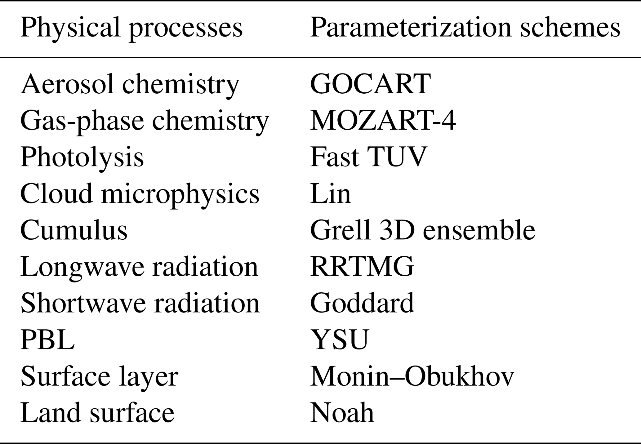
The model used in this study is an online coupled meteorology and chemistry model, WRF-Chem version 3.9.1 (Grell et al., 2005). The physics options used in WRF-Chem include the rapid radiative transfer model for general circulation models (RRTMG) for longwave radiation (Iacono et al., 2008), new Goddard shortwave radiation (Chou and Suarez, 1994), the Yonsei University (YSU) planetary boundary layer (PBL) scheme (Hong et al., 2006), the Lin microphysics scheme (Lin et al., 1983), and a new Grell 3D cumulus parameterization scheme. These options are chosen based on the operational configuration currently used in the Korean National Institute of Environmental Research (NIER) for their daily air quality forecasting in South Korea. The Goddard Chemistry Aerosol Radiation and Transport (GOCART; Chin et al., 2002), developed by the National Aeronautics and Space Administration (NASA), is used as an aerosol scheme. Aerosol direct effects are allowed through the interaction between GOCART and the Goddard shortwave radiation scheme (Fast et al., 2006; Barnard et al., 2010).
The Model for Ozone and Related Chemical Tracers (MOZART) gas-phase chemistry (Emmons et al., 2010) is generated with the kinetic preprocessor (KPP) (Damian et al., 2002; Sandu and Sander, 2006) and is used together with the simple GOCART aerosol scheme, known as the MOZCART mechanism (Pfister et al., 2011). The MOZART chemistry in WRF-Chem is designed to run with the Madronich FTUV scheme for photolysis processes (Tie et al., 2003), reading in climatological O3 and O2 overhead columns. It also utilizes the standard WRF-Chem implementation of the Wesley dry deposition scheme (based on Wesely, 1989) allowing for seasonal changes in the dry deposition. The resolved-scale wet scavenging is inactivated, but convective wet scavenging is applied in the Grell cumulus parameterization. Also, GOCART sea salt emissions and dust emissions with AFWA modifications (LeGrand et al., 2019) are included in this study.
Anthropogenic emissions are estimated offline based on the global EDGAR-Hemispheric Transport of Air Pollutants (HTAP) emission inventory (http://edgar.jrc.ec.europa.eu/htap_v2/, last access: 1 May 2018) that consists of grid maps of CH4, CO, SO2, NOx, NMVOC, NH3, PM10, PM2.5, BC, and OC from the year 2010. The emission data mapped to our model grids have a single level with no vertical variations and are generated from the annual mean with no diurnal variations (e.g., time-invariant). In terms of data range, the maximum (average) value of PM2.5 in the data, for example, is 3.56 (0.032) and 2.84 (0.026) µg m−2 s−1 in domain 1 and 2, respectively.
Biogenic emissions are built up using the Model of Emission of Gases and Aerosol from Nature (MEGAN; version 2) (Guenther et al., 2006), and for biomass burning emissions, daily fire estimates provided by the fire inventory from NCAR (FINN; Wiedinmyer et al., 2011) are used with tracer transport allowed. All the WRF files including biomass and biomass burning emissions are processed using the MODIS land use datasets (Friedl et al., 2002).
2.2 The GSI 3D-Var analysis system
2.2.1 Cost function
To assimilate AOD retrievals and surface PM2.5 observations in the Weather Research and Forecasting-Chemistry (WRF-Chem) model, the NCEP GSI 3D-Var version 3.5 system is used. As Liu et al. (2011) and Schwartz et al. (2012) described the details of the system for aerosol data assimilation, only a brief explanation follows. Incorporating observations into the three-dimensional model state space, a 3D-Var system produces the best estimate to the true state by minimizing the differences between observations and background forecasts (e.g., innovations; represented by o–b), which is called the “analysis”. The analysis is then used to initialize aerosol variables in the forecast model (e.g., WRF-Chem) so that the quality of aerosol forecasts can be largely dependent on the quality of the aerosol analysis produced in the 3D-Var system. Given the model state vector (x), the penalty function (or cost function) J(x) is defined as
where xb stands for the background state vector (e.g., forecasts from the previous cycle), and y is an observation vector. Here, the terms of background (b) and forecast (f) are used interchangeably throughout the paper; H is an observation operator that projects the model states onto the observation space linearly or nonlinearly to compute the model correspondent to each observation. Background and observation error covariance matrices B and R, respectively, indicate how reliable the background forecast (B in the first term) and the observed information (R in the second term) might be to determine how to properly weight the two disparate resources. By minimizing the cost function (J(x)) with respect to the model state vector x at the analysis time, the variational analysis algorithm produces the analysis that fits best to all the observations assimilated within the assimilation time window.
To characterize the forecast error magnitude and its spatial structure, background error covariance B is estimated for each aerosol species using the National Meteorological Center (NMC) method (Parrish and Derber, 1992) based on the differences between 48 and 24 h WRF-Chem forecasts valid at the same time for 30 samples ending at 00:00 UTC in May 2016. The current GSI/3D-Var system does not allow cross-correlation between aerosol species or between aerosol and meteorological variables. As this is a 3D-Var analysis with no time information, B only characterizes the spatial correlations in each analysis variable, which determines how to propagate the observed information across the model grids.
2.2.2 Observation operators
Following Liu et al. (2011) and Schwartz et al. (2012), this study also takes the speciated approach whereby the analysis vectors are comprised of 15 WRF-Chem/GOCART aerosol variables – sulfate, organic carbon and black carbon, mineral dust in five particle size bins (with effective radii of 0.5, 1.4, 2.4, 4.5, and 8.0 µm), sea salt in four particle size bins (with effective radii of 0.3, 1.0, 3.25, and 7.5 µm for dry air), and unspeciated aerosol contributions to PM2.5 – as opposed to using the total aerosol mass of PM2.5 as the analysis variable in Pagowski et al. (2010).
The observation operator H(x) for surface PM2.5 requires 10 GOCART aerosol variables as
where P represents unspeciated aerosol contributions to PM2.5; U denotes sulfate; O1 and O2 (B1 and B2) are hydrophobic and hydrophilic organic (black) carbon, respectively; and D1 and D2 (S1 and S2) are dust (sea salt) aerosols in the smallest and second-smallest size bins. This formula originated from the WRF-Chem diagnostics of PM2.5 for the GOCART aerosol scheme. PM observations are mass concentrations (µg m−3), while all the model variables listed within the bracket on the right-hand side are aerosol mixing ratios (µg kg−1); dry density ρd is thus required for the unit conversion in Eq. (2).
In this study, we assimilate AOD retrievals at 550 nm from both MODIS and GOCI sensors using the same observation operator based on the community radiative transfer model (CRTM; Han et al., 2006; Liu and Weng, 2006) as described in Liu et al. (2011). Although the GOCART aerosol scheme is well known to underestimate surface PM concentrations due to the lack of secondary organic aerosol (SOA) formation, nitrate, and ammonium (Liu et al., 2011; Volkamer et al., 2006; McKeen et al., 2009; Pang et al., 2018), it is widely used in analysis studies because it is the only scheme publicly available for assimilating AOD retrievals from satellite data in the GSI system. Aerosol optical depth (AOD) measures the amount of light extinction by aerosol scattering and absorption in the atmospheric column, which depends on the refractive indices and the size distribution of aerosol. In GSI, the CRTM computes the effective radii and the refractive indices of the 14 speciated WRF-Chem/GOCART aerosol species, assuming spherical aerosol particles and lognormal size distributions. Applying single-scattering properties of spheres by Mie theory, the mass extinction coefficient is computed as a function of the effective radius for each aerosol species at a certain wavelength (here, 550 nm) at each model level. The mass extinction coefficient (m2 g−1) for each aerosol species multiplied by the aerosol layer mass (g m−2) produces dimensionless AOD for the species at that level. To represent the entire atmospheric column, model-simulated AOD is then computed as the column integration of AOD for all aerosol species. Using the CRTM as a forward operator, AOD retrievals are assimilated separately or simultaneously with PM2.5 observations from the surface network over East Asia, as described in the following section.
During the month of May 2016, observations are assimilated in the GSI 3D-Var system to produce the analysis that is used as an initial condition for the following WRF-Chem simulations. WRF-Chem forecasts valid at the next analysis time are then used as a first guess (or background) for the next GSI analysis. In this study, the whole process is repeated every 6 h (called “cycled”) for the month-long period. Here we describe the analysis and the forecast systems used in the cycling.
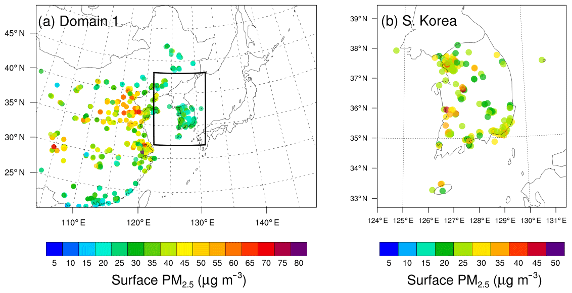
Figure 1Surface observation network with 960 Chinese stations and 361 Korean stations in domain 1 (a) and zoomed in over South Korea in (b). A black box in (a) indicates domain 2 over the Korean Peninsula. Dots indicate surface PM2.5 observations averaged over the month of May 2016.
3.1 Model configurations and cycling
All the analyses and the following forecasts are conducted over two one-way nested domains centered on the Korean Peninsula, as shown in Fig. 1. Domain 1 uses 175×127 horizontal grids at 27 km resolution, and domain 2 has 97×136 grids at 9 km resolution. Both domains have a total of 31 vertical levels up to 50 hPa. The initial and boundary meteorological conditions for domain 1 are provided by the UK Met Office Unified Model (UM-MET) global forecasts operated by the Korean Meteorological Administration (KMA) with a horizontal resolution of ∼25 km () at 26 isobaric levels every 6 h. This configuration was chosen due to the limitation of computational resources, but the use of higher resolutions both in time and space might be desirable to further improve forecast skills in the future. The chemical initial and boundary conditions for domain 1 are taken from the output of the global Model for Ozone and Related Chemical Tracers (MOZART-4) (Emmons et al., 2010) converted to WRF-Chem species by using the “mozbc” utility (downloaded from https://www2.acom.ucar.edu/wrf-chem/wrf-chem-tools-community/, last access: 28 November 2018). Meteorological and chemical fields in domain 1 are initialized from the global forecasts every cycle, while initial and boundary conditions for domain 2 are nested down from domain 1 in a one-way nesting. Aerosol and chemical initial conditions are then overwritten by WRF-Chem forecasts from the previous cycle in each domain. The GSI analysis is consecutively performed in the two domains using the same observations within each domain to update the initial conditions. During the cycles, 24 h forecasts are initialized from the 00:00 UTC analysis every day.
3.2 Observations
3.2.1 Surface PM2.5
Hourly surface PM concentrations are provided by the NIER, which collects real-time pollutant observations at 361 South Korean stations from AirKorea (http://www.airkorea.or.kr, last access: 11 September 2018) and those at ∼900 Chinese sites from the China National Environmental Monitoring Centre (CNEMC; http://www.cnemc.cn, last access: 31 October 2017). Figure 1 shows the entire surface observing network that was used to assimilate surface PM2.5. Observation sites are concentrated in the urban area where many sites are close enough to be overlapped with each other. The Seoul Metropolitan Area (SMA; centered around 37.5∘ N, 127∘ E), for example, has hourly reports from a total of 41 stations.
As part of data quality control (QC), surface PM2.5 concentrations higher than 100 µg m−3 are not assimilated, and observations producing innovations (represented as o–b) that exceed 100 µg m−3 were also discarded during the analysis step. To accommodate most measurements in China during heavy pollution events, a much higher threshold of 500 µg m−3 was once applied as the maximum observed value in our test experiment for the same month-long cycles, but it did not lead to any meaningful changes in the forecast performance over South Korea (not shown). Presumably this is because such high values were observed only over China where air pollutants were already overestimated by emission data based on the 2010 inventory such that the forecast skills over Korea became insensitive to the assimilation of those additional surface observations in China. Therefore, we applied the original threshold of 100 µg m−3 to all our experiments presented here.
Observation error is composed of measurement error (ϵo) and the representative error (ϵr) caused by the discrete model grid spacing (e.g., ). Following Elbern et al. (2007) and Schwartz et al. (2012), observation error for surface PM2.5 increases with the observed value (xo) as . The representative error is formulated as , where γ is 0.5, Δx is grid spacing (here, 27 km for domain 1 and 9 km for domain 2), and the scaling factor L is defined as 3 km. Based on this formula, observation error () ranges from 2.0 to 3.2 µg m−3 in domain 2, assigning the error of 2.48 µg m−3 to the PM2.5 observation of 50 µg m−3, for example. In this 3D-Var analysis, observation errors are considered to be uncorrelated so that the observation error covariance matrix R becomes diagonal. During the 6 h cycling, all the surface observations within a ±1 h window at each analysis time were assimilated without further adjustment of observation error.
3.2.2 AOD retrievals and observation preprocessing
Total AOD retrievals at 550 nm from MODIS sensors onboard the Terra and Aqua satellites have been widely used in aerosol studies (Zhang and Reid, 2006, 2010; Lee et al., 2011). But the polar-orbiting satellites produce a very limited dataset temporally (mostly around 06:00 UTC only) and spatially (with sparse coverage) over Korea during the KORUS-AQ period. The MODIS AOD level 2 products over both the land and ocean “dark” area are available at 10 km×10 km resolution and thinned over 60 km resolution during the GSI analysis in this study. Following Remer et al. (2005), observation errors are specified as the retrieval errors: () over ocean and () over land. They do not include the representativeness error and are slightly smaller than those for GOCI AOD, as described below.
The GOCI satellite monitors the East Asian region centered on the Korean Peninsula (36∘ N, 130∘ E), covering about 2500 km×2500 km. GOCI level II data have eight spectral bands from the visible to near-infrared range (412 to 865 nm) with hourly measurements during daytime from 09:00 (00:00 UTC) to 17:00 local time (08:00 UTC) at 6 km resolution. As summarized in Choi et al. (2018), a recently updated GOCI Yonsei aerosol retrieval (YAER) version 2 algorithm targets cloud- and snow-free pixels over land and cloud- and ice-free pixels over ocean in producing the level II data. By adopting the MODIS and VIIRS aerosol retrieval and cloud-masking algorithms, cloud pixels are filtered to avoid cloud contamination, and high-reflectance or highly heterogeneous reflectance pixels are also masked to further increase data accuracy and consistency during the retrieval process.
Unlike MODIS retrievals, GOCI AOD has not been extensively used in the data assimilation community. The GSI system takes most observation types in PrepBUFR format, which has already gone through some processing to be prepared for data assimilation, but the preprocessing algorithms are not publicly available. This means that when a new dataset is assimilated in GSI, users need to investigate the characteristics of the data (such as temporal and spatial distribution) and thereby make the data suitable for assimilation, which is of crucial importance for the analysis quality.
In terms of temporal distribution, most GOCI level II data are retrieved at 30 min past each hour in the hourly report. For example, the actual time for most of the data reported at 00:00 UTC is centralized around 00:30:00 UTC (hh:mm:ss). In the 3D-Var algorithm, there is no time dimension and all observations are considered to be available at the analysis time. To account for temporal distribution, different weights are often given to observations based on the relative distance between the actual report time and the analysis time during the analysis step. However, taking possible latency in data transfer and retrieval processing into consideration, it is not legitimate to assign weights to the retrievals based on their final report time without further information. Therefore, considering the high temporal and spatial variability of aerosols, the assimilation window is set to ±1 h in order to avoid inconsistent observed information within the window in this study.
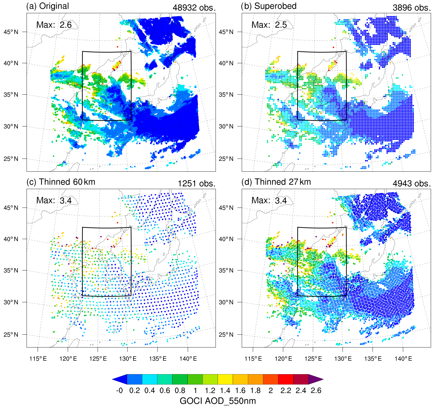
Figure 2Horizontal distribution of GOCI AOD at 550 nm retrieved at 06:00:00 UTC on 1 May 2016 in (a) the original level II data at 6 km resolution, (b) the preprocessed data at 27 km resolution before GSI, and the data thinned over (c) 60 km and (d) 27 km resolution during the GSI analysis. The total number of observations available for the GSI analysis is shown in the upper right corner of each panel, and the maximum value is in the upper left corner of each map. Domain 2 is marked as a black box in each panel.
Satellite data are known to have a large positive impact on the analysis quality thanks to the high data volume both in time and space, but such high density violates the assumption of uncorrelated observation errors in the analysis algorithm and increases the computation time for the analysis step excessively. Hence, a large volume of satellite retrievals are typically sampled on a regularly spaced grid through the horizontal thinning procedure. In GSI, satellite radiance data can be thinned such that retrievals are randomly sampled at a predefined spacing for each instrument type before being ingested into the observation operator during the analysis (Rienecker et al., 2008). This thinning procedure, however, can pick up inconsistent data (near the cloud boundaries, for instance) and is reported as suboptimal (Ochotta et al., 2005; Reale et al., 2018). Therefore, we decided to preprocess GOCI AOD retrievals with superobing whereby all the data points are averaged within a certain radius. In this study, we superobed GOCI retrievals over each grid box in domain 1 (at 27 km resolution). Figure 2 shows the sample horizontal distribution of GOCI AOD retrievals valid at 06:00 UTC on 1 May 2016 before (a) and after (b) preprocessing them, comparing with those thinned over 60 km (c) and 27 km meshes (d) during the GSI analysis, respectively. Some high AOD values in the original dataset (as shown in a), especially on cloud edges, cannot be fully resolved by our 27 km model grids. By averaging all data points over each grid box at 27 km resolution, the superobed data in (b) have a better quality control throughout the domain, reducing the data volume effectively. The total number of observations marked in the upper right corner of each panel indicates that thinning over the 60 km mesh in (c) reduces the number of assimilated observations to 2.5% of that in the original level II data, while superobing and thinning over the 27 km mesh utilize 8 %–10 % of the original data, representing the whole data coverage fairly well.
It might be noteworthy to make two more points related to data processing here. First, superobing was applied as part of preprocessing before the GSI analysis is started while, the thinning was conducted during the analysis step so that the preprocessing could speed up the GSI analysis up to 25 times (by injecting less than 10 % of the original data and turning off the thinning process). This can facilitate the use of satellite retrievals in operational air quality forecasting. Next, the thinning algorithm in GSI V3.5 resulted in erroneous values in some places, as indicated by the maximum values in (c) and (d). For the month of May 2016, multiple cases with such extreme fake values were found after the thinning process. This bug may need to be fixed in the GSI or avoided by bounding the values exceeding the original data.
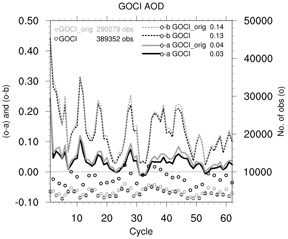
Figure 3Time series of observation minus analysis (o–a; solid lines) and observation minus background (o–b; dotted) with respect to GOCI AOD retrievals at 550 nm for two cycling experiments over domain 1. The GOCI_orig experiment assimilates the original data thinned over the 27 km mesh (in gray), while the GOCI experiment assimilates GOCI retrievals averaged over the 27 km grid mesh in domain 1 (black). Cycle-mean values are displayed next to each component. The total number of observations assimilated in each experiment at each cycle is also plotted as the “o” sign on the right y axis, ranging from 2000 to 12 000.
To examine the effect of data processing on the performance of the analysis and the background during the cycles, we compare two cycling experiments – one with the assimilation of the original level II data thinned over the 27 km mesh (named GOCI_orig in gray) and the other with the assimilation of GOCI retrievals preprocessed over the 27 km grids in domain 1 (called GOCI in black) – in Fig. 3. As GOCI data are reported from 00:00 to 08:00 UTC, only 00:00 and 06:00 UTC cycles are shown here in consecutive cycle numbers. The time series of (o–a) and (o–b) in each experiment show that the preprocessed data fit slightly better to the observations than the thinned data, assimilating more retrievals throughout the period. Because the differences between the two experiments are not significant, for computational efficiency, we decided to preprocess all the GOCI retrievals and assimilate them with the thinning process turned off in GSI for the rest of the experiments shown in this study.
Choi et al. (2018) described their improved retrieval algorithm (GOCI YAER V2) with updated cloud-masking and surface reflectance calculations, making a long-term evaluation against other ground- and satellite-based measurements. In their study, depending on the verifying objects – either ground-based Aerosol Robotic Network (AERONET) or satellite-based retrievals – they specified the uncertainties of GOCI AOD retrievals over land and ocean using two different linear regression formulae. We assign ϵ1 following their error specification with respect to AERONET and ϵ2 based on their expected error against retrieved satellite AOD in GOCI YAER V2.
Here, τA stands for GOCI AOD values. In an effort to account for representativeness error, we also tried with ϵ2 increased by 20 % everywhere as the third error formula (e.g., ) and compared all three types of errors in Fig. 4. When these different observation errors were applied to GOCI retrievals in the assimilation, the smallest error (ϵ2) produced slightly better fits to observations, especially for the high values (AOD >2) during the cycles, as expected, but not in a statistically meaningful way (not shown). In fact, it is not straightforward to estimate the representativeness error, which is subject to the model resolution (in the both horizontal and vertical) and data processing in use. Therefore, in many cases, observation error is specified based on the resulting forecast performance (Ha and Snyder, 2014). But because our forecast skills were not very sensitive to the three different error formulae tried here, for the rest of the experiments, ϵ2 is used as the observation error for GOCI retrievals.
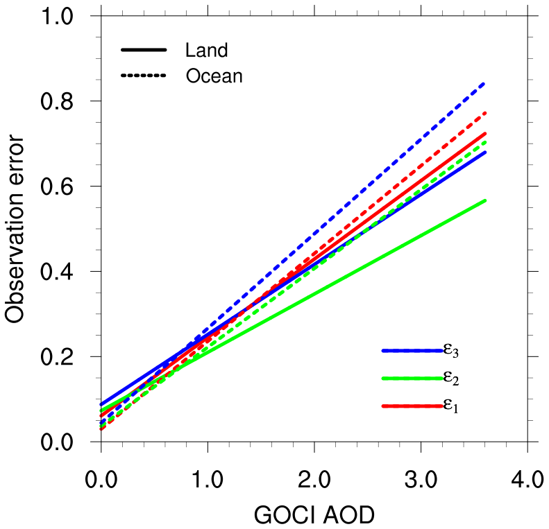
Figure 4Three different types of observation errors (ϵ) applied to GOCI AOD retrievals over land (solid line) and ocean (dashed line). The first two errors (ϵ1 and ϵ2) are described in Eqs. (3)–(6), and the third error (ϵ3) increases ϵ2 by 20 % everywhere.
The goal of this study is to examine the relative impact of the GOCI assimilation on the prediction of surface PM2.5 and ultimately to improve the forecasts for pollution events. Although it is rather easy to render the analysis close to GOCI observations by reducing the observation error, it is not guaranteed that the analysis in good agreement with AOD retrievals would actually lead to better forecasts in surface PM2.5. This is partly because AOD, a column-integrated quantity, is not directly associated with surface PM2.5 and partly because large uncertainties in the forecast model and the emission forcing can dominate over the analysis error during the model integration. Even if the efficiency of assimilating AOD toward improving surface PM2.5 forecasts can be largely affected by the quality of the forecast model and the emission data in use, the effectiveness of the AOD assimilation is based on the relationship between the column-integrated AOD and PM2.5 on the ground. Therefore, it might be worth checking the correlation between GOCI AOD retrievals and surface PM2.5 observations for the cycling period. Figure 5 depicts a scatter diagram of GOCI AOD retrievals at 550 nm and surface PM2.5 observations that are collocated in each grid box in domain 1 for the month of May 2016. As shown with the linear regression coefficient of 0.33, the two observation types have low correlations during this period, which is consistent with previous studies (Saide et al., 2014; Pang et al., 2018). Such an indirect relationship between the two observations makes the analysis challenging because it can induce a large error in the observation operator and heavily depends on the model's ability to derive PM2.5 from AOD based on the vertical structure of aerosol variables and the conversion from aerosol mass to optical properties.
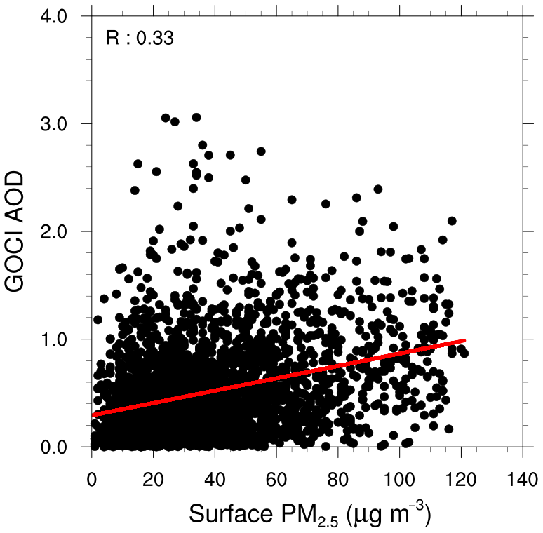
Figure 5Scatter plots of GOCI AOD retrievals versus ground PM2.5 observations collocated in domain 1 for the month of May 2016. The value of R is the correlation coefficient between the two observation types based on the linear regression shown as the red line.
With a careful design of the model configuration and observation processing, the overall impact of assimilating all the available observations (DA) is illustrated compared to the baseline experiment without data assimilation (NODA) in Fig. 6. Here, the 0–23 h hourly forecasts from all the 00:00 UTC analyses in domain 2 are concatenated for the entire month. Surface PM2.5 observations marked as black dots show that the air quality becomes distinctively aggravated for the last 7 d, which is related to the long-range transport of air pollutants. With data assimilation (DA), the analyses at 00:00 UTC and the following forecasts (red) are in better agreement with the corresponding observations than those without assimilation (gray), especially from day 15 (e.g., after a full spin-up for 2 weeks). In particular, on 25–27 May, forecast error grows quickly even from the good analysis at 00:00 UTC, possibly associated with large uncertainties in lateral boundary conditions and the forecast model in use. However, averaged over the entire period, the mean absolute error (MAE) indicates that the performance of 0–23 h forecasts at 9 km resolution is improved by ∼30 % through data assimilation.

Figure 6Time series of surface PM2.5 simulated with (DA; red) and without assimilation (NODA; gray) in domain 2, representing hourly 0–23 h forecasts from 00:00 UTC every day, as averages over 361 stations over South Korea. Corresponding observations are marked as black dots. The mean absolute error (MAE; |o–f|) averaged over the entire period is shown for each experiment. Here, DA refers to the ALL experiment.
4.1 Observation impact during the cycles
Given that the aerosol assimilation has a positive impact on air quality forecasting, it might be worth isolating the contribution of each observation type to the improvement of the analysis and the following forecasts. We first assimilate individual observation types separately, naming the experiment following each observation type, then we assimilate them all together (called ALL). Figure 7 illustrates the vertical profile of 10 three-dimensional GOCART aerosol variables that are used to diagnose PM2.5 in the GOCART scheme, the analysis (solid), and background (e.g., 6 h forecast; dashed) averaged over domain 2. Assuming that cycles may need to spin up meteorology and chemistry at least for 3 d in the regional simulations, all the statistics are computed from day 4 in the rest of the figures. Although the analysis variables only at the lowest model level are used in the observation operator for surface PM2.5, the observation impact is detected throughout the atmosphere due to the spatial correlations specified in the background error covariance. Contributions of different observations to each analysis variable vary, with the largest variability in the analysis increments (analysis minus background) displayed in sulfate. Interestingly, a large impact of AOD retrievals is noticed in hydrophilic organic carbon (O2) aloft (e.g., between 12 and 25 levels) and unspeciated aerosol (P) in the boundary layer. The assimilation of all the observations (ALL) tends to reduce O2, dust in both size bins (D1 and D2), and unspeciated aerosol (P) in the lower atmosphere.
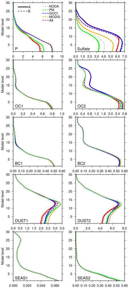
Figure 7Vertical profile of 10 GOCART aerosol variables composed of PM2.5 – unspeciated aerosol contributions to PM2.5 (P), sulfate, OC1 and OC2 (BC1 and BC2) as hydrophobic and hydrophilic organic (black) carbon, respectively, and DUST1 and DUST2 (SEAS1 and SEAS2) as dust (sea salt) aerosols in the smallest and second-smallest size bins. All the variables shown are mixing ratios ( µg kg−1). Different experiments are depicted in different colors, as averaged over domain 2 for the period of 4–31 May 2016. The analysis (A) is drawn as a solid line, while the background (e.g., 6 h forecast; B) is drawn as a dashed line.
Figure 8 summarizes the effect of different observations on PM2.5 in both domains. The assimilation of surface PM2.5 observations (green) results in the smallest PM2.5, while the GOCI assimilation (blue) produces the largest PM2.5 throughout the atmosphere in both domains. When the analysis (solid line) is compared to background (dashed), it is revealed that PM2.5 is predominantly increased over domain 1 with the assimilation of GOCI retrievals. Overall, the aerosol assimilation affects the entire profile of PM2.5, with the largest impact at the surface.
It is noted that the vertical distribution of the model aerosol species is associated with the vertical stratification of the model as well as the vertical distribution of the species in the background error covariance. It might be worth evaluating the vertical structure of individual species simulated in the model with respect to the vertical profiles observed during the KORUS-AQ field campaign (such as NASA DC-8 aircraft) in the future, although all the flight tracks were limited to the vicinity of the Korean Peninsula (Peterson et al., 2019).
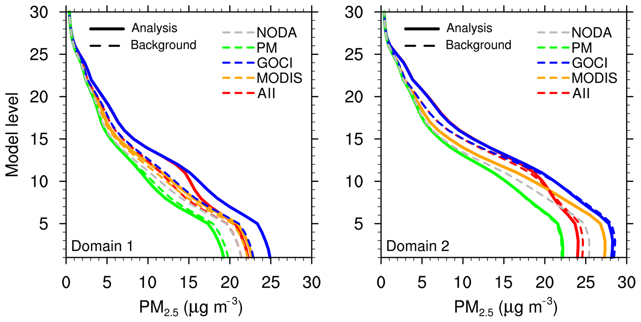

Figure 9Horizontal distribution of analysis increments (analysis minus background) in PM2_5_DRY, the model variable corresponding to PM2.5, at the lowest level in domain 1 averaged over the period of 4–31 May 2016. Maximum and mean values of the domain in each experiment are shown in the upper right corner of each panel.
To understand the observation impact in the horizontal distribution, Fig. 9 shows the analysis increments (analysis minus background) averaged over the period of 4–31 May 2016. Generally, the assimilation of surface PM2.5 observations (PM) reduces surface PM2.5 over most regions in China, while the GOCI assimilation largely increases surface PM2.5 almost everywhere, consistent with Fig. 8. As MODIS retrievals have a relatively low coverage of the East Asian region for the entire period, they have the smallest impact among all the observation types. When all the observations are assimilated together (in ALL), it combines the effect of surface PM2.5 and GOCI retrievals, changing the vertical distribution of aerosol species to match the AOD column values and pulling the surface states towards surface PM2.5 concentrations. While the observing network of surface PM2.5 is widely distributed over China, the impact of GOCI data is more centralized over Korea, making unequivocal contributions to air quality forecasting in the Korean Peninsula.
Note that we employ the 2010 inventory for our emission data, which does not reflect the emission control started from 2013 in China (Zheng et al., 2018). Given that air pollutants in the emission data constitute the majority of the precursors of PM2.5 pollution, surface PM2.5 concentrations could strongly depend on emissions, which might have led to the overestimation in the background (e.g., first guess). Therefore, the assimilation of surface PM2.5 tends to counteract the overestimation driven by the emission data over China. On the other hand, over South Korea, the emission data do not seem to be overestimated and the assimilation of surface PM2.5 leads to increasing surface PM2.5 most effectively during the cycles.
Different from surface particulate matter, AOD in the background is contingent upon the optical properties described in the observation operator (e.g., CRTM) and the vertical structure of aerosols simulated in the column. The influence of the GOCI assimilation may indicate model deficiencies in the two aspects because the model states are pulled toward the observed information during the analysis step, as depicted in the analysis increment.
Table 1Physical and chemical parameterizations used in the experiments.
4.2 Observation impact on 24 h forecasts
Since the real effect of data assimilation is manifested in the subsequent forecasts, we now examine forecast improvements when initialized by our own analyses. A good analysis is expected to slow down the forecast error growth, leading to better forecasts. In this subsection, forecast errors at the lowest model level are compared between experiments for 24 h with respect to surface observations from various sites in South Korea. As we focus on 9 km simulations over the Korean Peninsula, it is hard to anticipate the direct effect of the assimilation beyond 24 h, especially in such a small domain in which the weather systems dramatically change from day to day. As shown in Fig. 10, the forecast error is the largest in the baseline experiment (NODA), followed by the assimilation of MODIS retrievals alone (MODIS) in terms of mean absolute error (MAE). Note that the analysis in the PM experiment is verified against the same surface PM2.5 observations used in the assimilation. Therefore, the analysis error is smaller than those in other experiments, but the forecast error grows quickly over the next 24 h. The assimilation of surface PM2.5 alone generally underestimates the prediction of surface PM2.5, with the fastest growth of forecast error. On the other hand, the assimilation of AOD retrievals (either GOCI or MODIS) alone does not improve the surface analysis and mostly overestimates surface PM2.5 for 24 h.
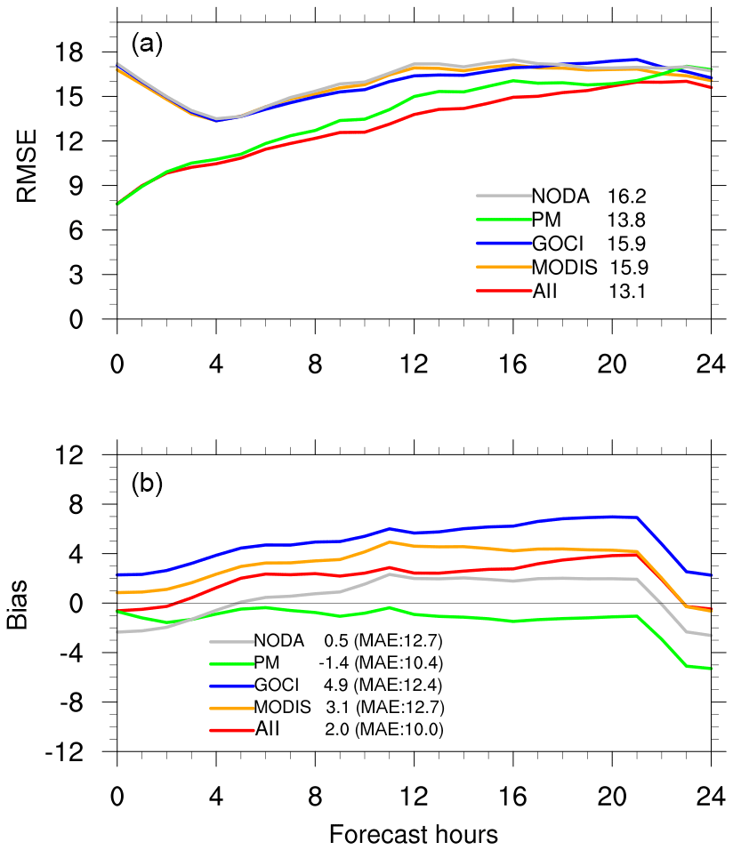
Figure 10Time series of root mean square error (RMSE; a) and bias (b) of the hourly forecasts from the 00:00 UTC initialization for 4–31 May 2016. Different experiments in domain 2 are verified against surface PM2.5 observations from 361 stations in South Korea. An average of 0–24 h forecast errors is shown next to each experiment name. The mean absolute error (MAE) over the 24 h forecasts is also shown in panel (b).
This might be ascribed to an imperfection of the forward operator of AOD and the model deficiency in the representation of three-dimensional aerosol species that comprised AOD and PM2.5. When assimilated with surface PM2.5 observations (in ALL), however, AOD retrievals effectively reduce the forecast error and suppress the error growth throughout 24 h forecasts.
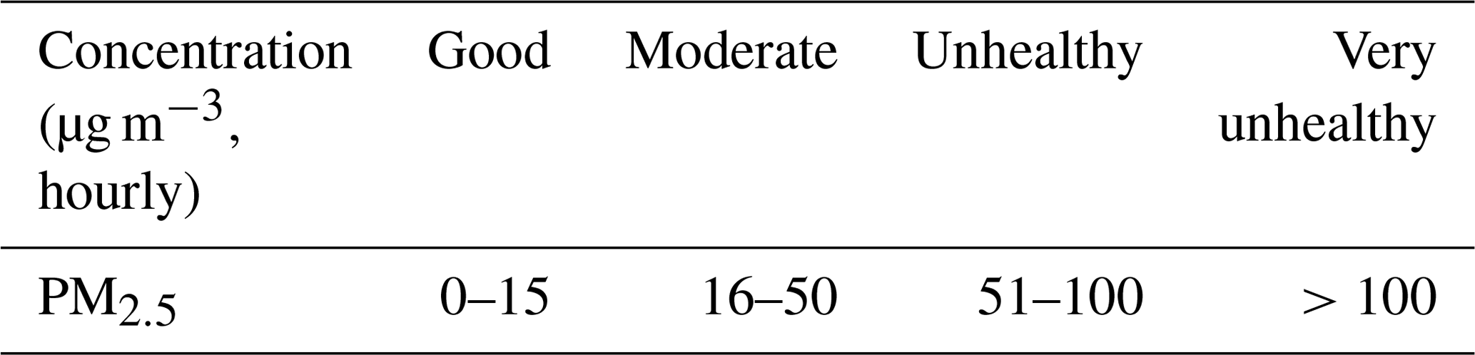
Table 3Categorical forecasts for different air pollution events.
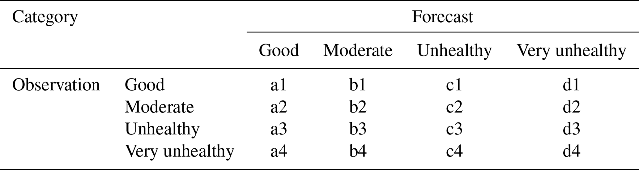
Recently, heavy pollution events have often taken place over Korea, and considerable attention has been drawn to the accuracy of operational air quality forecasting in the country, particularly in surface PM2.5. As accurately predicting exceedance and non-exceedance events in categorical predictions has great social impact, it is necessary to evaluate the forecast accuracy for different categorical events. While Miyazaki et al. (2019) classified the entire KORUS-AQ campaign period into four different phases based on dominant atmospheric circulation patterns, we categorize events for the month of May 2016 based on hourly surface PM2.5 concentrations, as summarized in Tables 2 and 3. Figure 11 summarizes the evaluation of 24 h forecasts based on the formulae described below.
Here, , , , and .
The air quality forecasting operated by the Korean NIER is currently evaluated in the same way on a daily basis, except for daily mean values.
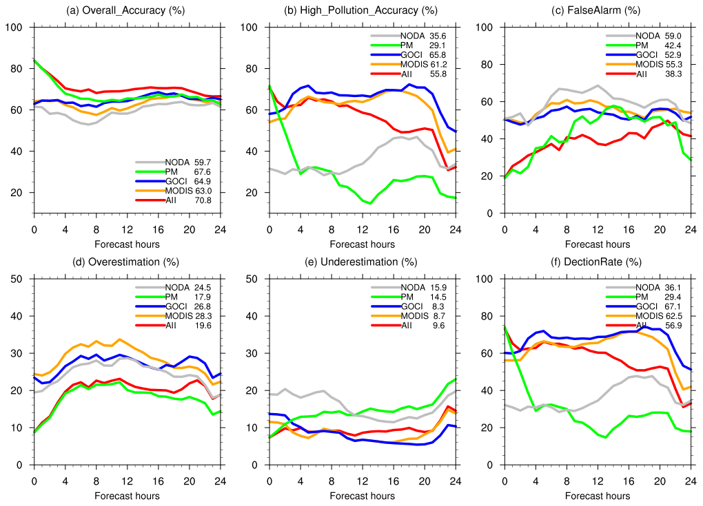
In all events, the overall accuracy of 0–24 h forecasts is the highest in ALL (∼70 %) and the lowest in NODA (∼60 %), which is about 10 % improvement through assimilation during this KORUS-AQ period. It is noted that the forecast error illustrated in Fig. 10 is dominated by days with a clear sky or moderate air quality conditions (about two-thirds of the month-long period, as shown in Fig. 6), while the forecast accuracy summarized in Fig. 11 is determined by equally weighting different categorical forecasts with different sample sizes. This implies that the categorical forecast evaluation tends to emphasize the forecast accuracy for pollution events (which has a smaller sample size). As such, Fig. 11a highlights the effect of data assimilation on improving air pollution forecasts. Differences between experiments are much larger in high pollution events (Fig. 11b) and the detection rate (Fig. 11f) to which AOD retrievals (both GOCI and MODIS) make the biggest positive contributions. While NODA produces poor forecasts consistently in most metrics shown in Fig. 11, the forecast accuracy in PM (green) drops very quickly for the first 12 h for all events (a) and pollution events (b), indicating that the assimilation of surface PM2.5 alone may not be enough to maintain the forecast skills beyond the cycling frequency (e.g., 6 h). It also increasingly underestimates surface PM2.5 with time, especially after 20 h, and produces more false alarms even though its overestimation rate is the lowest among all experiments. Overall, the AOD assimilation tends to overestimate the prediction of surface PM2.5 with a relatively large false alarm rate, but it clearly helps enhance the forecast accuracy up to 24 h when assimilated with surface PM2.5 observations. Even with low correlations with surface PM2.5 (as illustrated in Fig. 5), AOD retrievals keep the surface air pollution forecasts from drifting away from the true state, compensating for model deficiencies. This demonstrates that it could be substantially beneficial to monitor a wide range of the surrounding area using a geostationary satellite for the enhancement of air quality forecasts.
Table 4Forecast error in total AOD at 500 nm verified against AERONET sites, computed over 0–23 h forecasts from the 00:00 UTC analysis for 4–31 May.
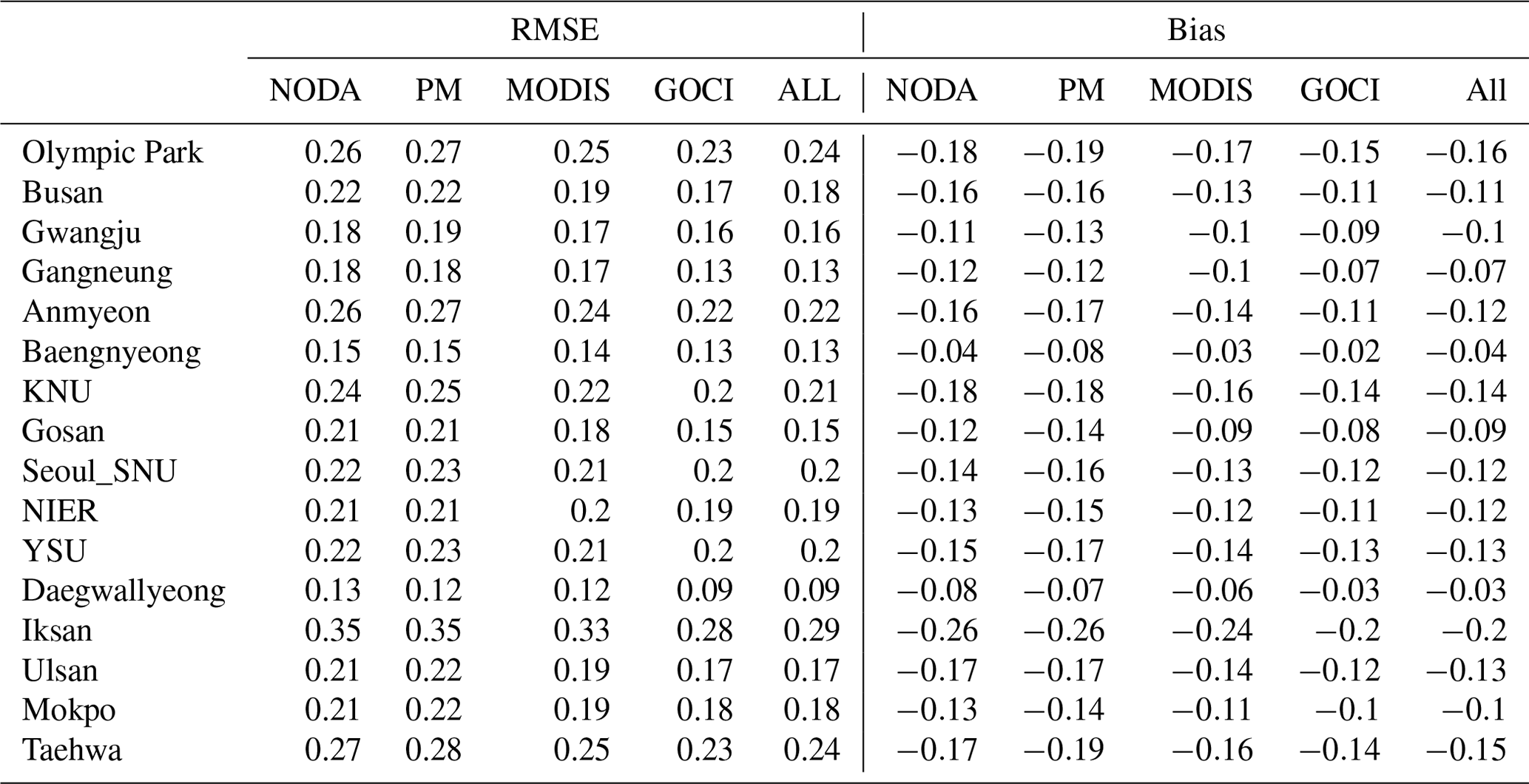
In order to verify our forecasts against independent observations, we processed total AOD at 500 nm from the Aerosol Robotic Network (AERONET; https://aeronet.gsfc.nasa.gov/, last access: 1 February 2019) sites and surface PM2.5 concentrations measured at three more stations operated by the NIER during the KORUS-AQ field campaign (Fig. 12). The level 2 data are used for AERONET AOD observations as cloud-free and quality-assured data. Figure 13 illustrates the time series of hourly AOD from our experiments compared to hourly averages of AOD observations from eight AERONET sites (black dots). At all sites, GOCI (blue) produces the largest AOD at most of the high peaks, while PM (green) and NODA (gray) simulate the smallest AOD throughout the period. Regardless of relative AOD values between the experiments, model forecasts are well matched with observations at low AOD values but mostly miss high AOD observations, especially during the high pollution events for 24–27 May. This leads to the negative mean bias (as f–o) in all experiments (shown in the legend), implying that our forecasts produce AOD slightly lower than the observed one as a whole. The RMSE and mean bias at a total of 16 AERONET sites are summarized in Table 4, indicating that GOCI has the smallest forecast error in AOD nationwide.
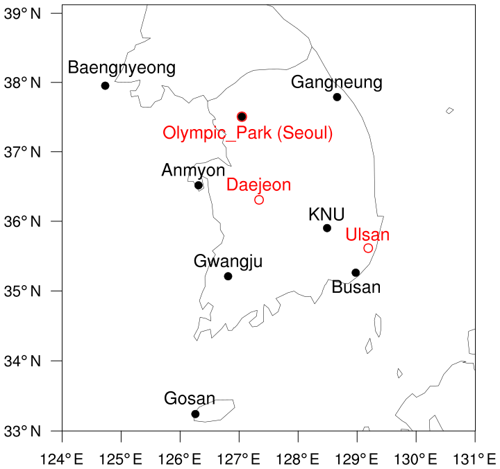
Surface PM2.5 measurements from three NIER sites were downloaded from https://www-air.larc.nasa.gov/cgi-bin/ArcView/korusaq (last access: 17 December 2019) as raw data with no quality control. They are provided as hourly averages starting from 9 May and compared to our hourly model output for 9–31 May (Fig. 14). These observations look somewhat noisy, but our forecasts broadly follow them throughout the period. Similar to the AOD verification shown in Fig. 13, forecasts from GOCI produce the smallest forecast mean bias among all the experiments in Olympic Park (a) and Daejeon (b), predicting high surface PM2.5 concentrations between 24 and 26 May. But GOCI was worse than other experiments in Ulsan (c), overestimating surface PM2.5, especially during high pollution days.
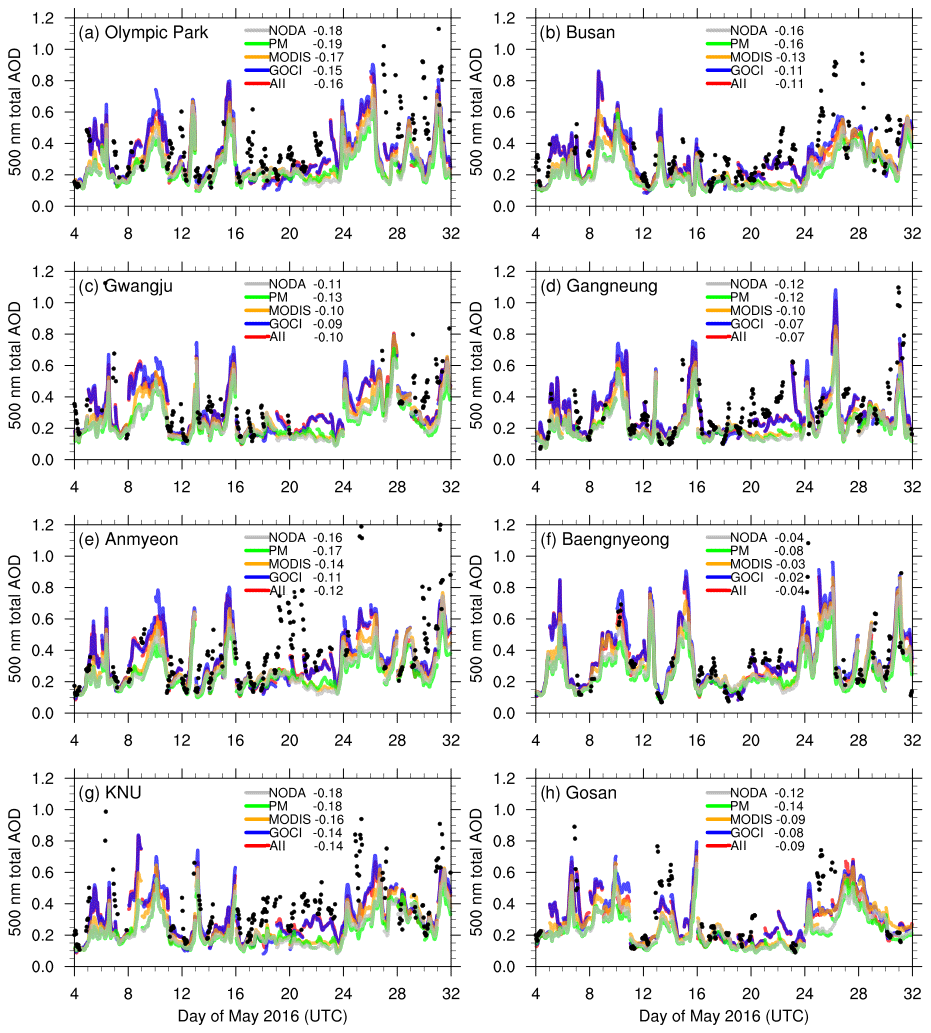
Figure 13Hourly time series of total AOD at 500 nm from 00:00 UTC on 4 May to 23:00 UTC on 31 May at eight different AERONET sites. Model values in different colors represent output every hour beginning at the initial time and ending at the 23rd hour of integration patched together for each 00:00 UTC forecast. The bias (represented as f–o) averaged over the entire period is shown next to each experiment name. AERONET observations represent hourly averages as black dots.

Figure 14Same as Fig. 13, but for surface PM2.5 concentrations from 00:00 UTC on 9 May to 23:00 UTC on 31 May at (a) Olympic Park in Seoul, (b) Daejeon, and (c) Ulsan. The sites are marked as red open dots in Fig. 12. The RMSE over the whole period is written next to each experiment name, along with the mean bias (represented as f–o) in parentheses.
In the assimilation system, raw data are not considered to be reliable, but this verification is included for completeness because there was no other instrument that reported surface PM2.5 concentrations or all the precursors of PM2.5 concentrations to validate PM2.5 forecasts on the ground level.
4.3 A heavy pollution case
The effect of assimilating different observations is most distinguishable in high pollution events, as demonstrated in Fig. 11. During the KORUS-AQ period, there were about five heavy pollution cases (when surface PM2.5>50 µg m−3, as defined in Table 2) over South Korea. The longest and the most severe pollution events occurred on 25–26 May 2016. Figure 15 illustrates how air pollutants were transported from China, associated with the strong synoptic weather systems in the region for a few days.
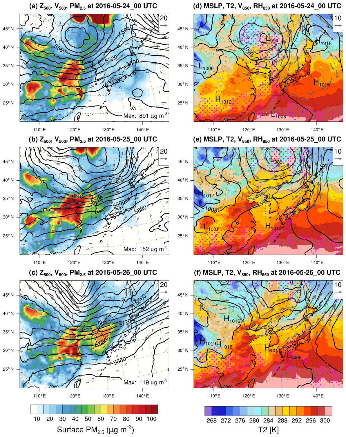
Figure 15The GSI 3D-Var analyses at 27 km resolution in domain 1 in the ALL experiment for 3 d from 24 to 26 May 2016 at 00:00 UTC (top to bottom). (a–c) The horizontal distribution of surface PM2.5 (µg m−3; filled), geopotential height (contours every 40 m), and horizontal winds (m s−1; gray vectors) at 500 hPa illustrates that the long-range transport of air pollution from China causes the heavy pollution over South Korea. (d–f) Mean sea level pressure (contours every 4 hPa), 2 m temperature (K; filled), relative humidity (>90 %; pink dots), and horizontal winds (m s−1; gray vectors) at 850 hPa represent the weather system in the low troposphere at the same time.
As the analysis of our best experiment ALL showed, the Korean Peninsula was positioned in the downstream region of the upper-level trough at 500 hPa (in the left panel). In the low troposphere, the center of the North Pacific High was situated in the east of Japan, bringing lots of moisture to Korea at 00:00 UTC on 24 May 2016 and blocking the eastward movement of the surface low-pressure system located north of Korea (centered around 46∘ N, 125∘ E), as shown in Fig. 15d. With the slowly approaching upper-level westerlies, these warm and moist conditions in the low troposphere provided a favorable environment for increasing air pollution in the Korean Peninsula for the next few days. At 00:00 UTC on 25 May, the Shangdong area in China (shown as the largest polluted area to the west of Korea) exceeded 150 µg m−3 in surface PM2.5 (Fig. 15b). This area has high topography with elevations higher than 3.5 km (in height above ground level; a.g.l.), while most regions in South Korea, especially the Seoul Metropolitan Area (SMA), are elevated near sea level. Therefore, when slow and deep baroclinic systems are approaching the Korean Peninsula like these events, a deep pool of highly polluted air can be advected from China as a whole to substantially degrade the air quality in South Korea at least for a day or two. This long-range transport case produced an hourly maximum surface PM2.5 observation of 117 µg m−3 over the SMA in Korea at 00:00 UTC on 26 May 2016, as shown in Fig. 16a.

Figure 16Horizontal distribution of 24 h forecast in 9 km simulations of PM2.5 at the lowest level in each experiment compared to (a) observations from 361 stations in South Korea valid at 00:00 UTC on 26 May 2016.
One notable difference between observations (a) and all the model simulations (b–f) in Fig. 16 is that 9 km forecasts driven by anthropogenic emissions cannot simulate such a high spatial variability across stations. During this heavy pollution event, there were dozens of missing observations, resulting in fewer stations in (a) than all the experiments (b–f). With only 145 stations reporting high concentrations (e.g., surface PM2.5>50 µg m−3), the observed distribution still shows a sharp gradient between the stations, especially in the SMA. Consistent with all the previous figures, the assimilation of surface PM2.5 alone (in PM) underpredicts surface PM2.5 (even more than NODA), while GOCI overpredicts surface PM2.5 the most among all observation types almost everywhere except for the SMA. MODIS retrievals slightly increase the concentrations from NODA (by ∼10 µg m−3), with the spatial distribution almost the same as that of NODA. In the concurrent assimilation of all the observations (in ALL), a moderate overestimation is presented everywhere, but higher levels of pollution in the SMA are not simulated either. To resolve such a large variability between urban and rural areas and to increase the sharpness of the forecast accuracy, the use of higher grid resolutions (such as 3 km), more accurate emission data, and more sophisticated aerosol chemistry mechanisms might be indispensable.
GOCI AOD retrievals provide reliable and consistent aerosol information, monitoring air pollutants over the Korean Peninsula at high resolution every day. One of the best ways of utilizing such invaluable observations is to inject them into the forecast system through data assimilation and better initialize numerical forecasts. For the successful assimilation of real observations, especially retrievals from satellites, extra attention should be paid to processing the data properly based on the characteristics. The spatial and temporal representativeness of GOCI retrievals was carefully examined and the corresponding data processing was conducted before assimilation in this study. We averaged all the pixels over each grid box at 27 km resolution (e.g., superobing) instead of thinning them randomly, for instance.
It is worth noting several challenges in the assimilation of AOD retrievals for improving the prediction of surface PM2.5 concentrations: (i) AOD is not directly associated with PM2.5 concentrations on the ground. Although the two datasets can be highly correlated in specific conditions such as cloud-free, low boundary layer heights, and low relative humidity, the overall correlation is low (∼0.3) in the present study and a direct impact on each other cannot be expected. (ii) An observation operator for AOD has errors due to the simplification and limited aerosol specifications in the community radiative transfer model (CRTM). (iii) There is significant model error, which is presumably one of the most critical issues. In the 3D-Var assimilation, in particular, the model estimates of AOD, a column-integrated quantity, are strongly constrained by the model error structure of each aerosol species both horizontally and vertically.
Even with these challenges, however, satellite-based AOD, especially from geostationary satellites like GOCI, can be extremely useful for improving the prediction of air pollution on a daily basis. In the situation in which air quality can be largely affected by the long-range transport of air pollutants, such consistent information on the wide upstream area is essential but hard to obtain otherwise.
Using the GSI 3D-Var system coupled with the WRF-Chem forecast model, we assimilated satellite AOD retrievals and surface PM2.5 observations for the month of May 2016 during the KORUS-AQ period. Compared to the baseline experiment (NODA), the simultaneous assimilation of various observations consistently improved the prediction of ground PM2.5 for 24 h forecasts, reducing systematic error and false alarms. The assimilation of ground PM2.5 alone improved the analysis during the cycles, reducing the analysis error to almost half the size compared to the experiment without assimilation. However, the forecast error grew very quickly over the next 12 h, underestimating PM2.5 at the surface, especially in heavy pollution events during which the forecast accuracy dropped from over 70 % to ∼30 % in only 4 h. Meanwhile, the GOCI AOD retrievals alone tended to overestimate surface PM2.5 but significantly contributed to improving air quality forecasts up to 24 h when assimilated with surface PM2.5 observations. The effect of data assimilation is most distinguishable and remarkable for high pollution events. During the month of May 2016, most heavy pollution events were associated with long-range transport from China. In such cases, it was particularly beneficial to monitor the wide upstream region using geostationary instruments such as GOCI.
To assess the effect of data assimilation with respect to independent observations, 0–23 h forecasts from different experiments are verified against AOD from AERONET sites and ground PM2.5 measurements from the sites operated during the KORUS-AQ field campaign. In this verification, the assimilation of GOCI retrievals is the most effective in improving the forecast performance at most sites, especially for high pollution events.
Even with successful data assimilation, there are several limitations in this study. First, the simple GOCART aerosol scheme is well known for the underestimation of air pollutants due to the lack of aerosol size distribution and secondary organic aerosol (SOA) formation. We had to use the scheme for the assimilation of AOD retrievals since the observation operator for AOD was only built for the GOCART scheme in the GSI system. Next, as there is no cross-covariance between aerosol and meteorological variables considered in the background error covariance estimates, the influence of aerosols on meteorological variables was not fully simulated in this study. Without the assimilation of meteorological observations, it was not possible to make an optimal estimate that is fully coupled between chemistry and meteorology, although the meteorological information was provided through the first guess and lateral boundary conditions. Finally, the emission inventory used in this study was based on the annual mean of 2010, which did not reflect the actual emissions for the year 2016, especially over China. The large bias and uncertainties in the emission data were particularly detrimental to the assimilation of surface PM2.5 alone.
To overcome the systematic underestimation of the GOCART aerosol scheme in the assimilation context, there is an ongoing effort for the development of a new interface for more sophisticated aerosol schemes such as MOSAIC and/or the Modal Aerosol Dynamics in Europe and the volatility basis set (MADE–VBS; Ackermann et al., 1998; Ahmadov et al., 2012) in the WRFDA system (Barker et al., 2012). This would be advantageous for more realistic forecast behavior in high-resolution applications.
The positive impact of data assimilation is generally limited to 24 h forecasts for three major reasons: first, most air pollutants have a short lifetime due to dry and wet deposition and transformations through interactions with solar radiation and clouds. Secondly, pollutant transport and transformations in chemical transport models are strongly driven by external forcing, such as emissions, boundary conditions, and meteorological fields. Lastly, there are large uncertainties in aerosol- and gas-phase chemistry parameterized in chemical transport models. Therefore, to extend the period of forecast improvements, emission data need to be improved, and large uncertainties in chemical and meteorological boundary conditions should be minimized. It has been shown that the estimation of emission inventories as part of the DA procedure can help extend the impact of data assimilation in longer forecasts (Elbern et al., 2007; Kumar et al., 2019). Also, more sophisticated aerosol and chemical mechanisms might be able to improve air quality forecasting by reducing model deficiencies (Chen et al., 2019). A simultaneous assimilation of meteorological observations and measurements of individual chemical species as well as particulate matter would certainly be beneficial in both NWP and air quality forecasting. To better account for high nonlinearities and uncertainties of aerosol forecasting on small scales, more advanced analysis techniques such as ensemble or hybrid data assimilation would be more desirable.
The WRF-Chem v3.9.1 codes are freely available from the University Corporation for Atmospheric Research (https://www2.mmm.ucar.edu/wrf/users/downloads.html, last access: 15 May 2020). The GSI v3.5 model codes are publicly available from the Developmental Testbed Center (https://dtcenter.org/com-GSI/users/downloads/index.php, last access: 15 May 2020).
ZL helped formulate the study, and WS performed initial test runs. YL and LC provided input datasets, partially funding this study. SH designed and ran the experiments, analyzed the results, and wrote the paper.
The authors declare that they have no conflict of interest.
All the experiments presented here were performed on the Cheyenne supercomputer at the National Center for Atmospheric Research (NCAR). This work was jointly supported by the National Science Foundation and the National Institute of Environment Research (NIER) funded by the Ministry of Environment (MOE) of the Republic of Korea. We acknowledge the use of the WRF-Chem preprocessor tool (mozbc, fire_emiss, megan_bio_emiss, and anthro_emiss) provided by the Atmospheric Chemistry Observations and Modeling Lab (ACOM) of NCAR. The authors are also grateful to Seunghee Lee, Ganghan Kim, and Myong-In Lee at UNIST in South Korea for their help transferring the input data for our experiments. Dave Gill and Wei Wang at MMM/NCAR helped us process data in WPS and tune the WRF configuration, respectively. Special thanks should go to Gabriele Pfister at ACOM/NCAR and Dan Chen at the China Meteorological Administration for their internal review, which greatly improved the paper. Two anonymous reviewers also helped to improve the clarify of the paper.
This research has been supported by the National Science Foundation (grant no. M0856145) and the Ministry of Environment (MOE) of the Republic of Korea (grant no. NIER-SP2018-252).
This paper was edited by Ilona Riipinen and reviewed by two anonymous referees.
Ackermann, I. J., Hass, H., Memmesheimer, M., Ebel, A., Binkowski, F. S., and Shankar, U.: Modal aerosol dynamics model for Europe: development and first applications, Atmos. Environ., 32, 2981–2999, https://doi.org/10.1016/S1352-2310(98)00006-5, 1998. a
Ahmadov, R., McKeen, S. A., Robinson, A. L., Bahreini, R., Middlebrook, A. M., de Gouw, J. A., Meagher, J., Hsie, E.-Y., Edgerton, E., Shaw, S., and Trainer, M.: A volatility basis set model for summertime secondary organic aerosols over the eastern United States in 2006, J. Geophys. Res.-Atmos., 117, D06301, https://doi.org/10.1029/2011JD016831, 2012. a
Baklanov, A., Schlünzen, K., Suppan, P., Baldasano, J., Brunner, D., Aksoyoglu, S., Carmichael, G., Douros, J., Flemming, J., Forkel, R., Galmarini, S., Gauss, M., Grell, G., Hirtl, M., Joffre, S., Jorba, O., Kaas, E., Kaasik, M., Kallos, G., Kong, X., Korsholm, U., Kurganskiy, A., Kushta, J., Lohmann, U., Mahura, A., Manders-Groot, A., Maurizi, A., Moussiopoulos, N., Rao, S. T., Savage, N., Seigneur, C., Sokhi, R. S., Solazzo, E., Solomos, S., Sørensen, B., Tsegas, G., Vignati, E., Vogel, B., and Zhang, Y.: Online coupled regional meteorology chemistry models in Europe: current status and prospects, Atmos. Chem. Phys., 14, 317–398, https://doi.org/10.5194/acp-14-317-2014, 2014. a
Baklanov, A., Brunner, D., Carmichael, G., Flemming, J., Freitas, S., Gauss, M., Hov, O., Mathur, R., Schlünzen, K. H., Seigneur, C., and Vogel, B.: Key Issues for Seamless Integrated Chemistry–Meteorology Modeling, B. Am. Meteorol. Soc., 98, 2285–2292, https://doi.org/10.1175/BAMS-D-15-00166.1, 2017. a
Barker, D., Huang, X.-Y., Liu, Z., Auligné, T., Zhang, X., Rugg, S., Ajjaji, R., Bourgeois, A., Bray, J., Chen, Y., Demirtas, M., Guo, Y.-R., Henderson, T., Huang, W., Lin, H.-C., Michalakes, J., Rizvi, S., and Zhang, X.: The Weather Research and Forecasting Model's Community Variational/Ensemble Data Assimilation System: WRFDA, B. Am. Meteorol. Soc., 93, 831–843, https://doi.org/10.1175/BAMS-D-11-00167.1, 2012. a
Barnard, J. C., Fast, J. D., Paredes-Miranda, G., Arnott, W. P., and Laskin, A.: Technical Note: Evaluation of the WRF-Chem ”Aerosol Chemical to Aerosol Optical Properties” Module using data from the MILAGRO campaign, Atmos. Chem. Phys., 10, 7325–7340, https://doi.org/10.5194/acp-10-7325-2010, 2010. a
Bocquet, M., Elbern, H., Eskes, H., Hirtl, M., Žabkar, R., Carmichael, G. R., Flemming, J., Inness, A., Pagowski, M., Pérez Camaño, J. L., Saide, P. E., San Jose, R., Sofiev, M., Vira, J., Baklanov, A., Carnevale, C., Grell, G., and Seigneur, C.: Data assimilation in atmospheric chemistry models: current status and future prospects for coupled chemistry meteorology models, Atmos. Chem. Phys., 15, 5325–5358, https://doi.org/10.5194/acp-15-5325-2015, 2015. a
Chang, L.-S., Cho, A., Park, H., Nam, K., Kim, D., Hong, J.-H., and Song, C.-K.: Human-model hybrid Korean air quality forecasting system, J. Air Waste Manage., 66, 896–911, https://doi.org/10.1080/10962247.2016.1206995, 2016. a
Chen, D., Liu, Z., Ban, J., Zhao, P., and Chen, M.: Retrospective analysis of 2015–2017 wintertime PM2.5 in China: response to emission regulations and the role of meteorology, Atmos. Chem. Phys., 19, 7409–7427, https://doi.org/10.5194/acp-19-7409-2019, 2019. a
Chin, M., Ginoux, P., Kinne, S., Torres, O., Holben, B., Duncan, B., Martin, R., Logan, J., Higurashi, A., and Nakajima, T.: Tropospheric Aerosol Optical Thickness from the GOCART Model and Comparisons with Satellite and Sun Photometer Measurements, J. Atmos. Sci., 59, 461–483, https://doi.org/10.1175/1520-0469(2002)059<0461:TAOTFT>2.0.CO;2, 2002. a
Choi, M., Kim, J., Lee, J., Kim, M., Park, Y.-J., Holben, B., Eck, T. F., Li, Z., and Song, C. H.: GOCI Yonsei aerosol retrieval version 2 products: an improved algorithm and error analysis with uncertainty estimation from 5-year validation over East Asia, Atmos. Meas. Tech., 11, 385–408, https://doi.org/10.5194/amt-11-385-2018, 2018. a, b, c
Chou, M.-D. and Suarez, M. J.: An efficient thermal infrared radiation parameterization for use in general circulation models, Tech. Memo 104606 [NTIS N95-15745], NASA, 1994. a
Damian, V., Sandu, A., Damian, M., Potra, F., and Carmichael, G. R.: The kinetic preprocessor KPP-a software environment for solving chemical kinetics, Comput. Chem. Eng., 26, 1567–1579, https://doi.org/10.1016/S0098-1354(02)00128-X, 2002. a
Elbern, H., Strunk, A., Schmidt, H., and Talagrand, O.: Emission rate and chemical state estimation by 4-dimensional variational inversion, Atmos. Chem. Phys., 7, 3749–3769, https://doi.org/10.5194/acp-7-3749-2007, 2007. a, b
Emmons, L. K., Walters, S., Hess, P. G., Lamarque, J.-F., Pfister, G. G., Fillmore, D., Granier, C., Guenther, A., Kinnison, D., Laepple, T., Orlando, J., Tie, X., Tyndall, G., Wiedinmyer, C., Baughcum, S. L., and Kloster, S.: Description and evaluation of the Model for Ozone and Related chemical Tracers, version 4 (MOZART-4), Geosci. Model Dev., 3, 43–67, https://doi.org/10.5194/gmd-3-43-2010, 2010. a, b
Fast, J. D., Gustafson Jr., W. I., Easter, R. C., Zaveri, R. A., Barnard, J. C., Chapman, E. G., Grell, G. A., and Peckham, S. E.: Evolution of ozone, particulates, and aerosol direct radiative forcing in the vicinity of Houston using a fully coupled meteorology-chemistry-aerosol model, J. Geophys. Res.-Atmos., 111, D21305, https://doi.org/10.1029/2005JD006721, 2006. a
Friedl, M., McIver, D., Hodges, J., Zhang, X., Muchoney, D., Strahler, A., Woodcock, C., Gopal, S., Schneider, A., Cooper, A., Baccini, A., Gao, F., and Schaaf, C.: Global land cover mapping from MODIS: algorithms and early results, Remote Sens. Environ., 83, 287–302, https://doi.org/10.1016/S0034-4257(02)00078-0, 2002. a
Grell, G. and Baklanov, A.: Integrated modeling for forecasting weather and air quality: A call for fully coupled approaches, Atmos. Environ., 45, 6845–6851, https://doi.org/10.1016/j.atmosenv.2011.01.017, 2011. a
Grell, G., Peckham, S., Schmitz, R., McKeen, S., Frost, G., Skamarock, W. C., and Eder, B.: Fully coupled “online” chemistry within the WRF model, Atmos. Environ., 39, 6957–6975, https://doi.org/10.1016/j.atmosenv.2005.04.027, 2005. a
Guenther, A., Karl, T., Harley, P., Wiedinmyer, C., Palmer, P. I., and Geron, C.: Estimates of global terrestrial isoprene emissions using MEGAN (Model of Emissions of Gases and Aerosols from Nature), Atmos. Chem. Phys., 6, 3181–3210, https://doi.org/10.5194/acp-6-3181-2006, 2006. a
Ha, S.-Y. and Snyder, C.: Influence of Surface Observations in Mesoscale Data Assimilation Using an Ensemble Kalman Filter, Mon. Weather Rev., 142, 1489–1508, https://doi.org/10.1175/MWR-D-13-00108.1, 2014. a
Han, Y., van Delst, P., Liu, Q., Weng, F., Yan, B., Treadon, R., and Derber, J.: JCSDA Community Radiative Transfer Model (CRTM) – Version 1, NOAA tech. rep. NESDIS 122, 2006. a
Hong, S.-Y., Noh, Y., and Dudhia, J.: A New Vertical Diffusion Package with an Explicit Treatment of Entrainment Processes, Mon. Weather Rev., 134, 2318–2341, https://doi.org/10.1175/MWR3199.1, 2006. a
Iacono, M. J., Delamere, J. S., Mlawer, E. J., Shephard, M. W., Clough, S. A., and Collins, W. D.: Radiative forcing by long-lived greenhouse gases: Calculations with the AER radiative transfer models, J. Geophys. Res., 113, D13103, https://doi.org/10.1029/2008JD009944, 2008. a
Jackson, J. M., Liu, H., Laszlo, I., Kondragunta, S., Remer, L. A., Huang, J., and Huang, H.-C.: Suomi-NPP VIIRS aerosol algorithms and data products, J. Geophys. Res.-Atmos., 118, 12673–12689, https://doi.org/10.1002/2013JD020449, 2013. a
Jiang, Z., Liu, Z., Wang, T., Schwartz, C. S., Lin, H.-C., and Jiang, F.: Probing into the impact of 3DVAR assimilation of surface PM10 observations over China using process analysis, J. Geophys. Res.-Atmos., 118, 6738–6749, https://doi.org/10.1002/jgrd.50495, 2013. a
Kalnay, E.: Atmospheric Modeling, Data Assimilation and Predictability, Cambridge Univ. Press, Cambridge, available at: http://cds.cern.ch/record/992314 (last access: 2 May 2018), 2003. a
Kim, J., Kim, M., and Choi, M.: Monitoring Aerosol Properties in East Asia from Geostationary Orbit: GOCI, MI and GEMS, 323–333, Springer International Publishing, Cham, https://doi.org/10.1007/978-3-319-59489-7_15, 2017. a
Kleist, D. T., D. F. Parrish, J. C. D., Treadon, R., Wu, W.-S., and Lord, S.: Introduction of the GSI into the NCEP Global Data Assimilation System, Weather Forecast., 24, 1691–1705, 2009. a
Kong, X., Forkel, R., Sokhi, R. S., Suppan, P., Baklanov, A., Gauss, M., Brunner, D., Barò, R., Balzarini, A., Chemel, C., Curci, G., Jiménez-Guerrero, P., Hirtl, M., Honzak, L., Im, U., Pérez, J. L., Pirovano, G., San Jose, R., Schlünzen, K. H., Tsegas, G., Tuccella, P., Werhahn, J., Z̆abkar, R., and Galmarini, S.: Analysis of meteorology-chemistry interactions during air pollution episodes using online coupled models within AQMEII phase-2, Atmos. Environ., 115, 527–540, https://doi.org/10.1016/j.atmosenv.2014.09.020, 2015. a
Kumar, R., Delle Monache, L., Bresch, J., Saide, P. E., Tang, Y., Liu, Z., da Silva, A. M., Alessandrini, S., Pfister, G., Edwards, D., Lee, P., and Djalalova, I.: Toward Improving Short-Term Predictions of Fine Particulate Matter Over the United States Via Assimilation of Satellite Aerosol Optical Depth Retrievals, J. Geophys. Res.-Atmos., 124, 2753–2773, https://doi.org/10.1029/2018JD029009, 2019. a
Lee, H. J., Liu, Y., Coull, B. A., Schwartz, J., and Koutrakis, P.: A novel calibration approach of MODIS AOD data to predict PM2.5 concentrations, Atmos. Chem. Phys., 11, 7991–8002, https://doi.org/10.5194/acp-11-7991-2011, 2011. a
Lee, J., Kim, J., Song, C. H., Ryu, J.-H., Ahn, Y.-H., and Song, C.: Algorithm for retrieval of aerosol optical properties over the ocean from the Geostationary Ocean Color Imager, Remote Sens. Environ., 114, 1077–1088, https://doi.org/10.1016/j.rse.2009.12.021, 2010. a
LeGrand, S. L., Polashenski, C., Letcher, T. W., Creighton, G. A., Peckham, S. E., and Cetola, J. D.: The AFWA dust emission scheme for the GOCART aerosol model in WRF-Chem v3.8.1, Geosci. Model Dev., 12, 131–166, https://doi.org/10.5194/gmd-12-131-2019, 2019. a
Lin, Y.-L., Farley, R. D., and Orville, H. D.: Bulk parameterization of the snow field in a cloud model, J. Clim. Appl. Meteorol., 22, 1065–1092, https://doi.org/10.1175/1520-0450(1983)022<1065:BPOTSF>2.0.CO;2, 1983. a
Liu, Q. and Weng, F.: Advanced Doubling-Adding Method for Radiative Transfer in Planetary Atmospheres, J. Atmos. Sci., 63, 3459–3465, https://doi.org/10.1175/JAS3808.1, 2006. a
Liu, Z., Liu, Q., Lin, H.-C., Schwartz, C. S., Lee, Y.-H., and Wang, T.: Three-dimensional variational assimilation of MODIS aerosol optical depth: Implementation and application to a dust storm over East Asia, J. Geophys. Res., 116, D23206, https://doi.org/10.1029/2011JD016159, 2011. a, b, c, d, e
McKeen, S., Grell, G., Peckham, S., Wilczak, J., Djalalova, I., Hsie, E.-Y., Frost, G., Peischl, J., Schwarz, J., Spackman, R., Holloway, J., de Gouw, J., Warneke, C., Gong, W., Bouchet, V., Gaudreault, S., Racine, J., McHenry, J., McQueen, J., Lee, P., Tang, Y., Carmichael, G. R., and Mathur, R.: An evaluation of real-time air quality forecasts and their urban emissions over eastern Texas during the summer of 2006 Second Texas Air Quality Study field study, J. Geophys. Res.-Atmos., 114, D00F11, https://doi.org/10.1029/2008JD011697, 2009. a
Miyazaki, K., Sekiya, T., Fu, D., Bowman, K. W., Kulawik, S. S., Sudo, K., Walker, T., Kanaya, Y., Takigawa, M., Ogochi, K., Eskes, H., Boersma, K. F., Thompson, A. M., Gaubert, B., Barre, J., and Emmons, L. K.: Balance of Emission and Dynamical Controls on Ozone During the Korea-United States Air Quality Campaign From Multiconstituent Satellite Data Assimilation, J. Geophys. Res.-Atmos., 124, 387–413, https://doi.org/10.1029/2018JD028912, 2019. a, b
Ochotta, T., Gebhardt, C., Saupe, D., and Wergen, W.: Adaptive thinning of atmospheric observations in data assimilation with vector quantization and filtering methods, Q. J. Roy. Meteor. Soc., 131, 3427–3437, https://doi.org/10.1256/qj.05.94, 2005. a
Pagowski, M., Grell, G. A., McKeen, S. A., Peckham, S. E., and Devenyi, D.: Three-dimensional variational data assimilation of ozone and fine particulate matter observations: some results using the Weather Research and Forecasting Chemistry model and Grid-point Statistical Interpolation, Q. J. Roy. Meteor. Soc., 136, 2013–2024, https://doi.org/10.1002/qj.700, 2010. a
Pang, J., Liu, Z., Wang, X., Bresch, J., Ban, J., Chen, D., and Kim, J.: Assimilating AOD retrievals from GOCI and VIIRS to forecast surface PM2.5 episodes over Eastern China, Atmos. Environ., 179, 288–304, https://doi.org/10.1016/j.atmosenv.2018.02.011, 2018. a, b, c
Parrish, D. F. and Derber, J. C.: The National Meteorological Center's spectral statistical-interpolation analysis system, Mon. Weather Rev., 120, 1747–1763, 1992. a
Peterson, D., Hyer, E., Han, S.-O., Crawford, J. H., Park, R., Holz, R., Kuehn, R., Eloranta, E., Knote, C., Jordan, C. E., and Lefer, B.: Meteorology influencing springtime air quality, pollution transport, and visibility in Korea, Elem. Sci. Anth., 7, 57, https://doi.org/10.1525/elementa.395, 2019. a
Pfister, G. G., Avise, J., Wiedinmyer, C., Edwards, D. P., Emmons, L. K., Diskin, G. D., Podolske, J., and Wisthaler, A.: CO source contribution analysis for California during ARCTAS-CARB, Atmos. Chem. Phys., 11, 7515–7532, https://doi.org/10.5194/acp-11-7515-2011, 2011. a
Reale, O., McGrath-Spangler, E. L., McCarty, W., Holdaway, D., and Gelaro, R.: Impact of Adaptively Thinned AIRS Cloud-Cleared Radiances on Tropical Cyclone Representation in a Global Data Assimilation and Forecast System, Weather Forecast., 33, 909–931, https://doi.org/10.1175/WAF-D-17-0175.1, 2018. a
Remer, L. A., Kaufman, Y. J., Tanré, D., Mattoo, S., Chu, D. A., Martins, J. V., Li, R.-R., Ichoku, C., Levy, R. C., Kleidman, R. G., Eck, T. F., Vermote, E., and Holben, B. N.: The MODIS Aerosol Algorithm, Products, and Validation, J. Atmos. Sci., 62, 947–973, https://doi.org/10.1175/JAS3385.1, 2005. a, b
Rienecker, M., Rienecker, M., Suarez, M. J., Todling, R., Bacmeister, J., Takacs, L., Liu, H.-C., Gu, W., Sienkiewicz, M., Koster, R. D., Gelaro, R., Stajner, I., and Nielsen, J. E.: The GEOS-5 Data Assimilation System: Documentation of versions 5.0.1, 5.1.0, and 5.2.0. NASA/TM-2008-104606, NASA Tech. Rep. Series on Global Modeling and Data Assimilation, Tech. Note NASA/TM-2008-104606, NASA, available at: https://ntrs.nasa.gov/search.jsp?R=20120011955 (last access: 9 November 2018), 2008. a
Saide, P. E., Kim, J., Song, C. H., Choi, M., Cheng, Y., and Carmichael, G. R.: Assimilation of next generation geostationary aerosol optical depth retrievals to improve air quality simulations, Geophys. Res. Lett., 41, 9188–9196, https://doi.org/10.1002/2014GL062089, 2014. a, b
Sandu, A. and Sander, R.: Technical note: Simulating chemical systems in Fortran90 and Matlab with the Kinetic PreProcessor KPP-2.1, Atmos. Chem. Phys., 6, 187–195, https://doi.org/10.5194/acp-6-187-2006, 2006. a
Schwartz, C. S., Liu, Z., Lin, H.-C., and McKeen, S. A.: Simultaneous three-dimensional variational assimilation of surface fine particulate matter and MODIS aerosol optical depth, J. Geophys. Res.-Atmos., 117, D13202, https://doi.org/10.1029/2011JD017383, 2012. a, b, c, d
Tie, X., Madronich, S., Walters, S., Zhang, R., Rasch, P., and Collins, W.: Effect of clouds on photolysis and oxidants in the troposphere, J. Geophys. Res.-Atmos., 108, 4642, https://doi.org/10.1029/2003JD003659, 2003. a
Volkamer, R., Jimenez, J. L., San Martini, F., Dzepina, K., Zhang, Q., Salcedo, D., Molina, L. T., Worsnop, D. R., and Molina, M. J.: Secondary organic aerosol formation from anthropogenic air pollution: Rapid and higher than expected, Geophys. Res. Lett., 33, L17811, https://doi.org/10.1029/2006GL026899, 2006. a
Wang, M., Ahn, J.-H., Jiang, L., Shi, W., Son, S., Park, Y.-J., and Ryu, J.-H.: Ocean color products from the Korean Geostationary Ocean Color Imager (GOCI), Opt. Express, 21, 3835–3849, https://doi.org/10.1364/OE.21.003835, 2013. a
Wesely, M.: Parameterization of surface resistances to gaseous dry deposition in regional-scale numerical models, Atmos. Environ., 23, 1293–1304, https://doi.org/10.1016/0004-6981(89)90153-4, 1989. a
Wiedinmyer, C., Akagi, S. K., Yokelson, R. J., Emmons, L. K., Al-Saadi, J. A., Orlando, J. J., and Soja, A. J.: The Fire INventory from NCAR (FINN): a high resolution global model to estimate the emissions from open burning, Geosci. Model Dev., 4, 625–641, https://doi.org/10.5194/gmd-4-625-2011, 2011. a
Wu, W.-S., Purser, R. J., and Parrish, D. F.: Three-Dimensional Variational Analysis with Spatially Inhomogeneous Covariances, Mon. Weather Rev., 130, 2905–2916, https://doi.org/10.1175/1520-0493(2002)130<2905:TDVAWS>2.0.CO;2, 2002. a
Xiao, Q., Zhang, H., Choi, M., Li, S., Kondragunta, S., Kim, J., Holben, B., Levy, R. C., and Liu, Y.: Evaluation of VIIRS, GOCI, and MODIS Collection 6 AOD retrievals against ground sunphotometer observations over East Asia, Atmos. Chem. Phys., 16, 1255–1269, https://doi.org/10.5194/acp-16-1255-2016, 2016. a
Zaveri, R. A., Easter, R. C., Fast, J. D., and Peters, L. K.: Model for Simulating Aerosol Interactions and Chemistry (MOSAIC), J. Geophys. Res.-Atmos., 113, D13204, https://doi.org/10.1029/2007JD008782, 2008. a
Zhang, J. and Reid, J. S.: MODIS aerosol product analysis for data assimilation: Assessment of over-ocean level 2 aerosol optical thickness retrievals, J. Geophys. Res.-Atmos., 111, D22207, https://doi.org/10.1029/2005JD006898, 2006. a
Zhang, J. and Reid, J. S.: A decadal regional and global trend analysis of the aerosol optical depth using a data-assimilation grade over-water MODIS and Level 2 MISR aerosol products, Atmos. Chem. Phys., 10, 10949–10963, https://doi.org/10.5194/acp-10-10949-2010, 2010. a
Zheng, B., Tong, D., Li, M., Liu, F., Hong, C., Geng, G., Li, H., Li, X., Peng, L., Qi, J., Yan, L., Zhang, Y., Zhao, H., Zheng, Y., He, K., and Zhang, Q.: Trends in China's anthropogenic emissions since 2010 as the consequence of clean air actions, Atmos. Chem. Phys., 18, 14095–14111, https://doi.org/10.5194/acp-18-14095-2018, 2018. a