the Creative Commons Attribution 4.0 License.
the Creative Commons Attribution 4.0 License.
 | 06 Apr 2020
Bromine from short-lived source gases in the extratropical northern hemispheric upper troposphere and lower stratosphere (UTLS)
Timo Keber
Harald Bönisch
Carl Hartick
Marius Hauck
Fides Lefrancois
Florian Obersteiner
Akima Ringsdorf
Nils Schohl
Tanja Schuck
Ryan Hossaini
Phoebe Graf
Patrick Jöckel
Andreas Engel
We present novel measurements of five short-lived brominated source gases (CH2Br2, CHBr3, CH2ClBr, CHCl2Br and CHClBr2). These rather short-lived gases are an important source of bromine to the stratosphere, where they can lead to depletion of ozone. The measurements have been obtained using an in situ gas chromatography and mass spectrometry (GC–MS) system on board the High Altitude and Long Range Research Aircraft (HALO). The instrument is extremely sensitive due to the use of chemical ionization, allowing detection limits in the lower parts per quadrillion (ppq, 10−15) range. Data from three campaigns using HALO are presented, where the upper troposphere and lower stratosphere (UTLS) of the northern hemispheric mid-to-high latitudes were sampled during winter and during late summer to early fall. We show that an observed decrease with altitude in the stratosphere is consistent with the relative lifetimes of the different compounds. Distributions of the five source gases and total organic bromine just below the tropopause show an increase in mixing ratio with latitude, in particular during polar winter. This increase in mixing ratio is explained by increasing lifetimes at higher latitudes during winter. As the mixing ratios at the extratropical tropopause are generally higher than those derived for the tropical tropopause, extratropical troposphere-to-stratosphere transport will result in elevated levels of organic bromine in comparison to air transported over the tropical tropopause. The observations are compared to model estimates using different emission scenarios. A scenario with emissions mainly confined to low latitudes cannot reproduce the observed latitudinal distributions and will tend to overestimate organic bromine input through the tropical tropopause from CH2Br2 and CHBr3. Consequently, the scenario also overestimates the amount of brominated organic gases in the stratosphere. The two scenarios with the highest overall emissions of CH2Br2 tend to overestimate mixing ratios at the tropical tropopause, but they are in much better agreement with extratropical tropopause mixing ratios. This shows that not only total emissions but also latitudinal distributions in the emissions are of importance. While an increase in tropopause mixing ratios with latitude is reproduced with all emission scenarios during winter, the simulated extratropical tropopause mixing ratios are on average lower than the observations during late summer to fall. We show that a good knowledge of the latitudinal distribution of tropopause mixing ratios and of the fractional contributions of tropical and extratropical air is needed to derive stratospheric inorganic bromine in the lowermost stratosphere from observations. In a sensitivity study we find maximum differences of a factor 2 in inorganic bromine in the lowermost stratosphere from source gas injection derived from observations and model outputs. The discrepancies depend on the emission scenarios and the assumed contributions from different source regions. Using better emission scenarios and reasonable assumptions on fractional contribution from the different source regions, the differences in inorganic bromine from source gas injection between model and observations is usually on the order of 1 ppt or less. We conclude that a good representation of the contributions of different source regions is required in models for a robust assessment of the role of short-lived halogen source gases on ozone depletion in the UTLS.
- Article
(6103 KB) - Full-text XML
-
Supplement
(63321 KB) - BibTeX
- EndNote


Following the detection of the ozone hole during springtime over Antarctica (Farman et al., 1985) and the attribution of the decline in both polar and global ozone to the emissions of anthropogenic halogenated compounds (see Molina and Rowland, 1974; Solomon, 1999; Engel and Rigby, 2018), production and use of long-lived halogenated species, in particular chlorofluorocarbons (CFCs), have been regulated by the Montreal Protocol (WMO, 2018). This has led to decreasing levels of chlorine in the atmosphere (Engel and Rigby, 2018), despite recent concerns over ongoing emissions of CFC-11, which have been attributed to unreported and thus illegal production (Montzka et al., 2018; Engel and Rigby, 2018; Rigby et al., 2019). Bromine reaching the stratosphere has been identified as an even stronger catalyst for the depletion of stratospheric ozone than chlorine (Wofsy et al., 1975; Sinnhuber et al., 2009). Its relative efficiency on a per molecule basis is currently estimated to be 60–65 times larger than that of chlorine (see discussion in Daniel and Velders, 2006). Long-lived bromine gases include CH3Br with partly natural and partly anthropogenic sources and halons, which are of purely anthropogenic origin. Next to long-lived gases, some chlorine and bromine from so-called “very-short-lived substances” (VSLS), i.e. substances with atmospheric lifetimes less than 6 months, can reach the stratosphere. It has been estimated that, for the year 2016, about 25 % of the bromine entering the stratosphere is from VSLS (Engel and Rigby, 2018). Due to the decline in chlorine and bromine from long-lived species, the relative contribution of short-lived species to stratospheric halogen loading is expected to increase, which is also driven by increasing anthropogenic emissions of some short-lived chlorinated halocarbons (Hossaini et al., 2017, 2019; Oram et al., 2017; Leedham Elvidge et al., 2015; Engel and Rigby, 2018).
A number of factors control the abundance of ozone at mid latitudes, including influences from dynamics, chemical destruction, aerosol loading and the solar cycle (e.g. Feng et al., 2007; Harris et al., 2008; Dhomse et al., 2015). In the lowermost stratosphere, the breakdown of VSLS provides a significant bromine source in a region where (a) ozone loss cycles involving bromine chemistry are known to be important (e.g. Salawitch et al., 2005) and (b), on a per molecule basis, ozone perturbations have a relatively large radiative effect (Hossaini et al., 2015). At present, VSLS are estimated to supply a total of ∼5 (3–7) ppt (parts per trillion, 10−12) Br to the stratosphere, with source gas injection estimated to provide 2.2 (0.8–4.2) ppt Br and product gas injection 2.7 (1.7–4.2) ppt Br (Engel and Rigby, 2018). Attribution of lower stratospheric ozone trends is complex and trends in this region are highly uncertain (Steinbrecht et al., 2017; Ball et al., 2018; Chipperfield et al., 2018). It has been suggested that continuing negative ozone trends observed in the lower stratosphere (defined as about 13 to 24 km in the mid latitudes) may partly be related to increasing anthropogenic and natural VSLS (Ball et al., 2018). While Chipperfield et al. (2018) suggested that the main driver for variability and trends in lower stratospheric ozone is dynamics rather than chemistry, the bromine budget of the upper troposphere and lower stratosphere (UTLS) needs to be well understood.
In the past, the main focus of upper tropospheric bromine studies for VSLS has been on the tropics, as this is the main entry region for air masses to reach above 380 K potential temperatures (see discussion in Engel and Rigby, 2018) and thus for the main part of the stratosphere. However, as many authors have shown, the lowermost stratosphere, i.e. the part of the stratosphere situated below 380 K but above the extratropical stratosphere, is influenced by transport from the tropics and from the extratropics (e.g. Holton et al., 1995; Gettelman et al., 2011; Fischer et al., 2000; Hoor et al., 2005). Some authors have quantified the fraction of air in the lowermost stratosphere, which did not pass the tropical tropopause, from tracer measurements (Hoor et al., 2005; Bönisch et al., 2009; Ray et al., 1999; Werner et al., 2010) and others have used trajectory analyses to study mass fluxes and stratosphere–troposphere exchange (e.g. Stohl et al., 2003; Wernli and Bourqui, 2002; Škerlak et al., 2014; Appenzeller et al., 1996). Based on tracer measurements of mainly CO, Hoor et al. (2005) estimated that the fraction of air with extratropical origin in the mid-latitude lowermost stratosphere of the Northern Hemisphere ranged between about 35 % during winter and spring to about 55 % during summer and fall. Using a different approach based on CO2 and SF6 observations, Bönisch et al. (2009) found a similar seasonality but higher extratropical fractions, which were consistently higher than 70 % during summer and fall and above 90 % in the entire lowermost stratosphere during October. Similarly, Bönisch et al. (2009) also derived much lower fractions of air with recent extratropical origin during winter and spring, which were sometimes as low as 20 % during April. It has also been argued that the relative role of different source regions for the UTLS could alter with a changing circulation (Boothe and Homeyer, 2017).
Both extratropical and tropical source regions are important for the lowermost stratosphere. A recent compilation of entry mixing ratios of brominated VSLS to the stratosphere (Engel and Rigby, 2018) has focused on mixing ratios representative of the tropical tropopause. Two pathways for input of halogens from short-lived gases are discussed. Halogen atoms can be transported to the stratosphere in the form of the organic source gas (source gas injection (SGI)) or in the inorganic form as photochemical breakdown products of source gases (product gas injection (PGI)). Halogens from product gases are readily available for catalytic ozone depletion reactions. Source gases have to undergo a photochemical transformation into inorganic bromine, which can then interact with ozone. Due to the short lifetimes of VSLS, this release is expected to occur in the lowest part of the stratosphere. Therefore, brominated VSLS are particularly effective with respect to ozone chemistry in the lower and lowermost stratosphere, below about 20 km, with the associated ozone decreases exerting a significant radiative effect (Hossaini et al., 2015). It has been shown that observed and modelled ozone show a better agreement if bromine from short-lived species is included in models (Sinnhuber and Meul, 2015; Fernandez et al., 2017; Oman et al., 2016). In particular for the Antarctic ozone hole, an enhancement in size by 40 % and an enhancement in mass deficit by 75 % was simulated due to VSLS (Fernandez et al., 2017) in comparison with a model run without VSLS. A delay in polar ozone recovery by about a decade has also been reported due to the inclusion of brominated VSLS (Oman et al., 2016). In order to have solid projections on the effect of VSLS on ozone and climate, a good knowledge of their atmospheric distribution is thus needed for models.
Observations indicate that the main source of brominated VSLS is from oceans and in particular from coastal regions. Four global emission scenarios of short-lived brominated gases have been proposed (Warwick et al., 2006; Ordóñez et al., 2012; Ziska et al., 2013; Liang et al., 2010), with variations in VSLS source strengths of more than a factor of 2 between them (Engel and Rigby, 2018). In the past, these scenarios have been compared to each other and to observations; large differences have been identified in modelled tropospheric mixing ratios of CHBr3 and CH2Br2, along with estimates of stratospheric bromine input (Hossaini et al., 2013, 2016; Sinnhuber and Meul, 2015). Hossaini et al. (2013) concluded that the lowest suggested emissions of CHBr3 (Ziska et al., 2013) and the lowest suggested emissions of CH2Br2 (Liang et al., 2014) yielded the overall best agreement in the tropics and thus the most realistic input of stratospheric bromine from VSLS. They also concluded that “Averaged globally, the best agreement between modelled CHBr3 and CH2Br2 with long-term surface observations made by NOAA/ESRL is obtained using the top-down emissions proposed by Liang et al. (2010)”. It has also been proposed that VSLS emissions may have increased by 6 %–8 % between 1979 and 2013 (Ziska et al., 2017), although no observational evidence for this has been found (Engel and Rigby, 2018). A further future increase has been suggested (Ziska et al., 2017; Falk et al., 2017), although this projection is very uncertain and the processes associated with the oceanic production of brominated VSLS are still poorly understood. It has also been proposed that certain source regions could be more effective with respect to transport to the stratosphere, in particular the Indian Ocean, the Maritime Continent and the tropical western Pacific (Liang et al., 2014; Fernandez et al., 2014; Tegtmeier et al., 2012). The Asian monsoon has also been named as a possible pathway for transport of bromine from VSLS to the stratosphere (Liang et al., 2014; Fiehn et al., 2017; Hossaini et al., 2016).
While most investigations of natural VSLS focused on tropical injection of bromine to the stratosphere, this study focuses on the extratropical bromine VSLS budget. In order to investigate the regional variability of bromine input into the lowermost stratosphere, we have performed a range of airborne measurement campaigns using an in situ gas chromatograph (GC) coupled to a mass spectrometer (MS) on board the High Altitude and Long Range Research Aircraft (HALO). The differences in stratospheric inorganic bromine from observations and from models are discussed. In Sect. 2 we give a brief introduction to the instrument, the available observations and the models used for this study. Typical distributions of brominated VSLS derived from these observations are then presented in Sect. 3 and compared to model output from two different atmospheric models run with the different emission scenarios mentioned above in Sect. 4. Finally, in Sect. 5 the implications of the observations for inorganic bromine in the stratosphere are discussed.
2.1 Instrumentation and observations
The data presented here have been measured with the in situ Gas chromatograph for Observational Studies using Tracers – Mass Spectrometer (GhOST-MS) deployed on board HALO. GhOST-MS is a two-channel GC instrument. An electron capture detector (ECD) is used in an isothermal channel in a similar set-up as used during the SPURT campaign (Bönisch et al., 2009, 2008; Engel et al., 2006) to measure SF6 and CFC-12 with a time resolution of 1 min. The second channel is temperature programmed and uses a cryogenic pre-concentration system (Obersteiner et al., 2016; Sala et al., 2014) and a mass spectrometer (MS) for detection. It is similar to the set-up described by Sala et al. (2014) and measures halocarbons in the chemical ionization mode (e.g. Worton et al., 2008) with a time resolution of 4 min. As explained in Sala et al. (2014), CH2BrCl2 and CH2Br2 are not separated chromatographically during normal measurements with GhOST-MS, as this would require too much time. Instead, a correlation between the two species from either independent measurements or measurements of the two species from dedicated flights are used. Such dedicated flights have been performed during the WISE and PGS campaigns (defined below). The procedure of how CHBrCl2 and CH2Br2 are derived from the single chromatographic peak with this additional information is explained in Sala et al. (2014). While CH4 has been used as chemical ionization gas for the TACTS campaign (defined below) and for the tropical measurements discussed in Sala et al. (2014), a change in chemical ionization gas was necessary for later measurements due to safety reasons. During the PGS campaign pure Argon was used, which resulted in very good sensitivities but also an interference with water vapour. In order to avoid this interference for the mid-latitude (more humid) measurements during WISE, a mixture of Argon and methane (non-burnable, below 5 % methane) was used as ionization gas. These (and some other) changes resulted in different performances of the instrument during different campaigns. Typical performance details of the instrument are given for the WISE and PGS campaigns in Table 1 for the brominated hydrocarbons.
The instrument is tested for non-linearities, memory and blank signals, which are corrected where necessary (see the description in Sala, 2014, and Sala et al., 2014, for details). Table 1 also includes typical local lifetimes of the different VSLS species and the global lifetimes of the long-lived species. The instrument was deployed during several campaigns of the German research aircraft HALO, providing observations in the UTLS over a wide range of latitudes and different seasons mainly in the Northern Hemisphere. Some observations from the Southern Hemisphere are also available, but, due to their sparsity, they will not be part of this work.
Table 1Brominated species measured with Gas chromatograph for Observational Studies using Tracers – Mass Spectrometer (GhOST-MS) during three High Altitude and Long Range Research Aircraft campaigns, described in Table 2. Tropospheric mole fractions (parts per trillion, ppt; 10−12) of the halons are taken from Table 1-1 in Engel and Rigby (2018) and from Table 1-7 for the bromocarbons (marine boundary layer value mixing ratios). Lifetimes of bromocarbons are local lifetimes for upper tropospheric conditions (10 km altitude, 25–60∘ N) from Table 1-5 in Carpenter and Reimann (2014) and global/stratospheric lifetimes are from Table A-1 in WMO 2018 (Burkholder, 2018). Local lifetimes are given in days (d), while global and stratospheric lifetimes are given in years (yr). Reproducibilities and detection limits of GhOST have been determined during the WISE and the PGS campaigns. For the TACTS campaign instrument, performance was similar to that reported in Sala et al. (2014).

n/a: not applicable.
GhOST-MS measurements from three HALO missions will be presented and discussed here. The first atmospheric science mission of HALO was TACTS (Transport and Composition in the Upper Troposphere/Lowermost Stratosphere), conducted between August and September 2012, with a focus on the Atlantic sector of the mid latitudes of the Northern Hemisphere. The second campaign was PGS, a mission consisting of three sub-missions: POLSTRACC (Polar Stratosphere in a Changing Climate), GW-LCYCLE (Investigation of the Life cycle of gravity waves) and SALSA (Seasonality of Air mass transport and origin in the Lowermost Stratosphere). PGS took place mainly in the Arctic between December 2015 and March 2016. Finally, the GhOST-MS was deployed during the WISE (Wave-driven ISentropic Exchange) mission between September and October 2017. The dates of the missions and some parameters on the available observations are summarized in Table 2, and the flight tracks are shown in Figs. 1 and 2. As the WISE and TACTS campaigns covered a similar time of the year and latitude range, the data from the two campaigns have been combined into a single dataset, which we will refer to as “WISE_TACTS”. Vertical profiles of the two major bromine VSLS, CH2Br2 and CHBr3, for the TACTS and WISE campaigns are shown separately in Fig. S1 in the Supplement. For this combined dataset, some observations from the TACTS campaign have been omitted, where some extremely high values of VSLS (up to a factor of 10 above typical tropospheric mixing ratios) were observed in the UTLS, which are suspected of being contaminated. The source of the contamination is, however, unknown. Figure 3 shows an example time series of halon 1301 (CF3Br), CH2Br2 and CHBr3, ozone and mean age of air calculated from the SF6 measurements obtained during a typical flight in the Arctic in January 2016. It is clearly visible that the halocarbons are correlated amongst each other, whereas they are anticorrelated with ozone and mean age. It is further evident from Fig. 3 that the shortest-lived halocarbon measured by GhOST-MS, i.e. CHBr3, decreases much faster with increasing ozone than the longer-lived CH2Br2 or the long- lived source gas halon 1301. Note that the local lifetimes of the halocarbons may differ significantly from their typical mid-latitude lifetimes shown in Table 1. Lifetimes generally increase with (a) decreasing temperature for species with a sink through the reaction with the OH radical and (b) with decreasing solar irradiation for species with direct photolytic sink. Therefore, in particular during winter, lifetimes are estimated to increase considerably with increasing latitude due to the decreased solar illumination and low temperatures.
Table 2Brief description of measurement campaigns with the High Altitude and Long Range Research Aircraft (HALO) used for this study.
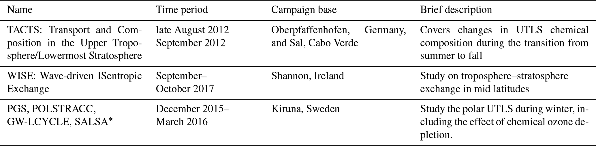
* PGS is a synthesis of three measurement campaigns: POLSTRACC (The Polar Stratosphere in a Changing Climate), GW-LCYCLE (Investigation of the Life cycle of gravity waves) and SALSA (Seasonality of Air mass transport and origin in the Lowermost Stratosphere).

Figure 1Flight tracks of HALO during the (a) TACTS campaign (late August and September 2012) and (b) WISE campaign (September–October 2017). The basis of the TACTS campaign was mainly Oberpfaffenhofen (near Munich in Germany), while the basis of the WISE campaign was Shannon (Ireland).

Figure 2Flight tracks of HALO during the PGS campaign (December 2015 to April 2016). The basis of the campaign was mainly Kiruna in northern Sweden.
2.2 Models and meteorological data
Data from two different models were used in this study: ESCiMo (Earth System Chemistry Integrated Modelling) data from the EMAC (ECHAM/MESSy Atmospheric Chemistry) chemistry climate model (CCM) and the TOMCAT (Toulouse Off-line Model of Chemistry And Transport) chemistry transport model (CTM).
For EMAC data, we used results from the simulations in the so-called specified dynamics (SD) mode, for which the model was nudged (by Newtonian relaxation) towards ERA-Interim meteorological reanalysis data from the European Centre for Medium-Range Weather Forecasts (ECMWF; Dee et al., 2011). T42 spectral model resolution was used, corresponding to a quadratic Gaussian grid of approximately 2.8∘ by 2.8∘ horizontal resolution, and the vertical resolution comprised 90 hybrid sigma-pressure levels up to 0.01 hPa. The model output has been subsequently interpolated to pressure levels between 1000 and 0.01 hPa. The emissions of VSLS were taken from the emission scenario 5 in Warwick et al. (2006). The EMAC SD simulations with 90 vertical levels, as described in detail by Jöckel et al. (2016), were integrated with an internal model time step length of 12 min, and the data have been output every 10 h from which the monthly averages on pressure levels have been derived. The SC1SD-base-01 simulation, which has been used here, has been branched off from RC1SD-base-10 (see Jöckel et al., 2016) at 1 January 2000 using the RCP8.5 emissions and greenhouse gas scenario.
The TOMCAT model (Chipperfield, 2006; Monks et al., 2017) is driven by analysed wind and temperature fields taken 6-hourly from the ECMWF ERA-Interim product. Here, the model was run with T42 horizontal resolution (2.8∘ by 2.8∘) and with 60 vertical levels, extending from the surface to ∼60 km. The internal model time step was 30 min, and tracers were output as monthly means. This configuration of the model has been used in a number of VSLS-related studies and is described by Hossaini et al. (2019). In this study, three different VSLS emission scenarios are used with TOMCAT (Liang et al., 2010; Ordóñez et al., 2012; Ziska et al., 2013). In the case of the Liang et al. (2010) scenario, their scenario A has been used. Chemical breakdown by reaction with OH and photolysis in the model for all VSLS (CHBr3, CH2Br2, CH2BrCl, CHBr2Cl and CHBrCl2) are calculated using the relevant kinetic data from Burkholder et al. (2015).
Local tropopause information for the flights with HALO have been derived from ERA-Interim data. The climatological tropopause has been calculated based on potential vorticity (PV) according to the method described in Škerlak et al. (2015) and Sprenger et al. (2017) based on the ERA-Interim reanalysis. As the PV tropopause is not physically meaningful in the tropics, the level with a potential temperature of 380 K has been adapted for the tropopause where the 2 PVU (potential vorticity unit) level is located above the 380 K level.
Spatial distributions are shown in tropopause-relative coordinates and as functions of equivalent latitude. As equivalent latitude is mainly a useful horizontal coordinate for the stratosphere, we chose to use standard latitude for all measurements below the tropopause and equivalent latitude for all measurements above the tropopause. We refer to this coordinate as equivalent latitude*. As the observations typically cover a range of latitudes, vertical profiles are shown for 20∘ bins. In the vertical direction, three different coordinates are used in this paper. These are potential temperature θ, potential temperature above the local tropopause Δ θ and finally a coordinate we refer to as θ∗, which is calculated by adding the potential temperature of the mean tropopause to Δ θ. We used the dynamical tropopause, defined by a potential vorticity of 2 PVU or by a potential temperature of 380 K in the tropics (see Sect. 2), as a reference surface.
3.1 Mean vertical profiles
All measurements from the individual campaigns have been binned into 10 K potential temperature bins between −40 and 100 K of Δθ. For potential temperature binning, the 10 K bins have been chosen ranging from 40 K below the mean tropopause to 100 K above the mean tropopause. In this way, the centres of the Δθ and θ bins are the same relative to the mean tropopause observed during the measurements. The results are presented for the two main VSLS bromine source gases CH2Br2 and CHBr3, averaged over equivalent latitude* of 40–60∘ N in Fig. 4 for PGS (northern hemispheric winter) and the WISE_TACTS combined dataset (late summer to fall, Northern Hemisphere). Results for the minor VSLS and total organic bromine are shown in Figs. S2 and S3. Only bins which contain at least five data points have been included in the analysis. The results are also summarized in Tables 3 and 4 for the same latitude intervals for all species and for total organic bromine derived from the five brominated VSLS. The tropopause mole fractions shown in Tables 3 and 4 have been derived as the average of all values in that latitude interval and within 10 K below the tropopause. The potential temperature of the average tropopause has been used for θ averaging, while the potential temperature difference to the local tropopause has been used as reference when averaging in Δθ coordinates. Due to this different sampling, a higher range in Δθ is achieved than in θ, as the actual tropopause altitude varies. We have checked the validity of using means to represent the data, by comparing means and medians. Differences were always below 5 % of the mean tropopause mixing ratios. We have thus chosen to use means throughout this paper. The uncertainties given in all figures are 1σ standard deviations of these means, both for the vertical and horizontal error bars. In the WISE_TACTS dataset, total organic bromine at the dynamical tropopause between 40 and 60∘ N was 4.05 and 3.5 ppt, using Δθ and θ as vertical coordinates, respectively. Higher mixing ratios of total organic bromine were found during the winter campaign PGS, when average tropopause mixing ratios were 5.2 and 4.9 ppt both using Δθ and θ as vertical coordinates. These mixing ratios are considerably higher than the tropical tropopause values of organic bromine derived in the vicinity of the tropical tropopause (Engel and Rigby, 2018) as will be discussed in detail below. When using the WMO definition of the tropopause, the total organic bromine at mid latitudes was lower by up to 0.5 ppt than using the PV tropopause, reflecting the fact that the WMO tropopause is usually slightly higher than the dynamical tropopause using the 2 PVU definition (e.g. Gettelman et al., 2011).
Table 3Averaged mole fractions (parts per trillion, ppt; 10−12) and vertical gradients of brominated very-short-lived substances from the combined WISE and TACTS dataset, representative of 40–60∘ N during late summer to early fall (data from late August to October). Data have been averaged using potential temperature, θ, and potential temperature difference to the tropopause, Δθ, as vertical profile coordinates. Tropopause (TP) mixing ratios are from the 10 K bin below the dynamical tropopause (see text for details). The 10 K bin standard deviations in the table represent the variability averaged over the four lowest stratospheric bins. The average potential temperature of the tropopause during the WISE and TACTS campaigns has been calculated from the European Centre for Medium-Range Weather Forecasts data at the locations of our measurements.
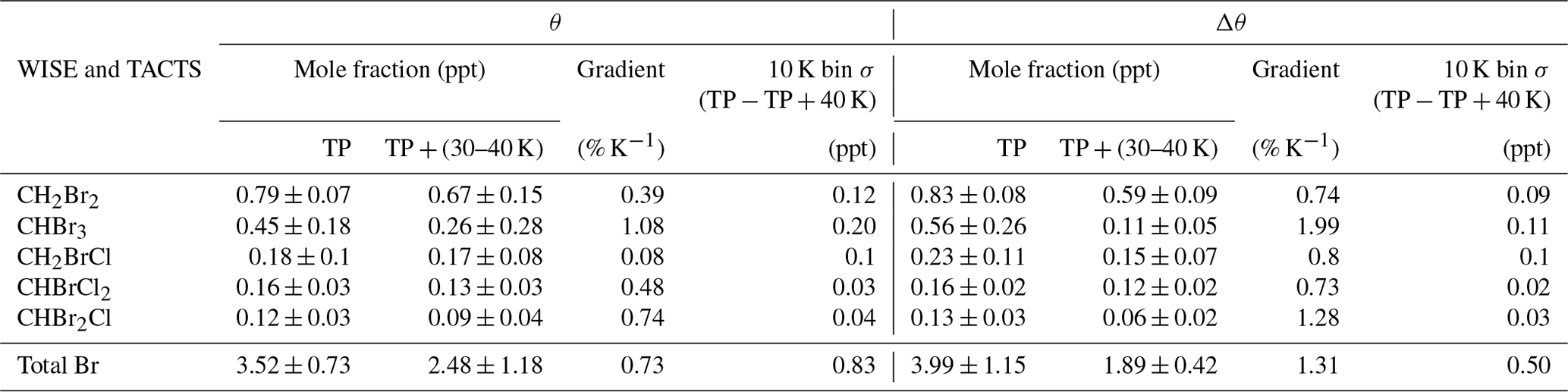
Table 4Averaged mole fractions and vertical gradients of brominated VSLS during the PGS campaign. Data have been averaged using potential temperature, θ, and potential temperature difference to the tropopause, Δθ, as vertical profile coordinates. Tropopause (TP) mixing ratios are from the 10 K bin below the dynamical tropopause (see text for details). The 10 K bin standard deviations in the table represent the variability averaged over the four lowest stratospheric bins. The average potential temperature of the tropopause during the PGS campaign has been calculated from ECMWF data at the locations of our measurements.
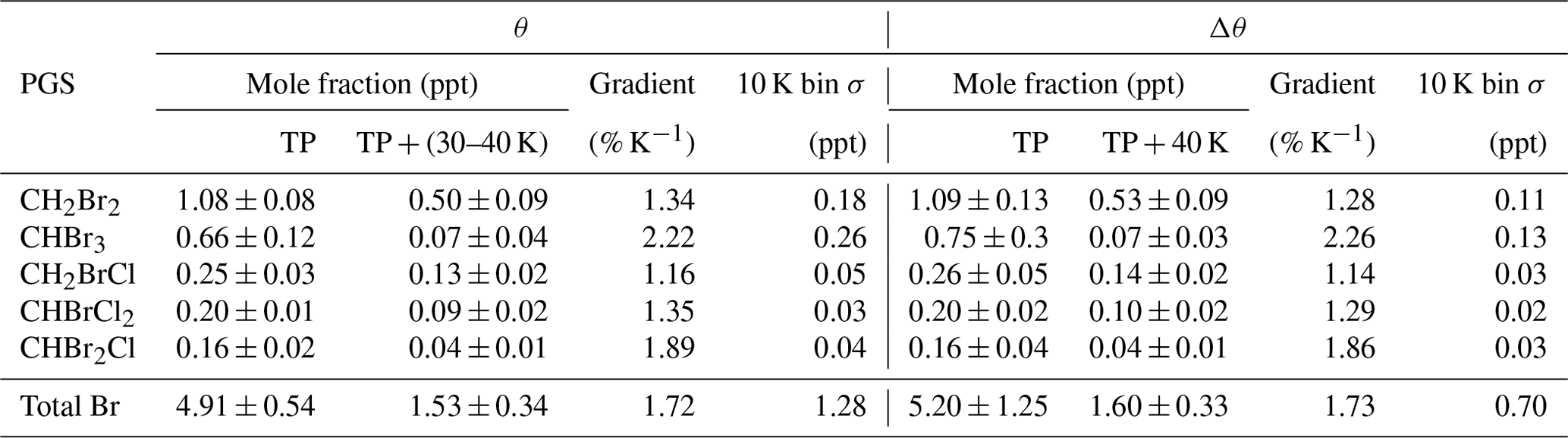
CHBr3 showed the largest vertical gradients of all species discussed here, followed by CHBr2Cl. This is well in line with their atmospheric lifetimes (see Table 1), which will generally decrease with an increase in bromine atoms in the molecule and is shortest for CHBr3, followed by CHBr2Cl. The relationship between lifetime and vertical gradient is less clear for the longer-lived species, where vertical profiles are expected to be more influenced by transport. In particular, the vertical gradient of CHBrCl2 is closer to the vertical gradient of CH2Br2 than to that of CHBr2Cl, although the lifetime should be closer to CHBr2Cl. This could be related to the way that CHBrCl2 is derived, as it is not chromatographically separated from CH2Br2 (see Sect. 2.1 and Sala et al., 2014). The strongest vertical gradients with respect to both θ and Δθ were observed during the winter campaign PGS, with the exception of CHBr3, which was nearly completely depleted for all campaigns at 40 K above the tropopause and thus shows very similar averaged gradients over this potential temperature region. When evaluated only for the first 20 K above the tropopause, the gradient of CHBr3 was also much larger during PGS then during WISE and TACTS. The short lifetime and strong vertical gradient of CHBr3 is also reflected in the largest relative variability (see Tables 3 and 4).
We further determined the variability of the different species in 10 K intervals of θ and Δθ. For all campaigns, the variability averaged over the four lowest stratospheric bins when using Δθ was always lower than in the four lowest bins above the climatological tropopause using θ as a coordinate (see Tables 3 and 4). This shows that using the tropopause-centred coordinate system Δθ reduces the variability in the stratosphere, and it is therefore the best suited coordinate system to derive typical distributions. In the troposphere, the variability is larger when using Δθ coordinates than for θ, indicating that the variability in the free troposphere is not influenced by the potential temperature of the tropopause. The observed variabilities were found to be very similar for the WMO and PV tropopause definitions (not shown). As the dynamical PV tropopause is generally expected to be better suited for tracer studies, we decided to reference all data to the dynamical tropopause.
3.2 Latitude–altitude cross sections
We slightly diverge from the coordinate system used to present zonal mean latitude–altitude distributions used in previous work (e.g. Bönisch et al., 2011; Engel et al., 2006), where equivalent latitude and potential temperature were used as horizontal and vertical coordinates. We use equivalent latitude* as a horizontal coordinate, i.e. latitude for all tropospheric observations and equivalent latitude for observations at or above the tropopause. As a vertical coordinate we have chosen to use a modified potential temperature coordinate θ∗ (see explanation above, Sect. 3). In this way, all measurements are presented relative to a climatological tropopause, which has been derived from ERA-Interim reanalysis as zonal mean for the latitude of interest and the specific months of the campaign (see Sect. 2 for campaign details). This is expected to reduce variability by applying the information from Δθ, yet the absolute vertical information is also maintained. In order to ensure that this tropopause value is representative also of the period of our observations, we compare the potential temperature of the campaign-based tropopause with the climatological tropopause. The campaign-based tropopause has been calculated by averaging the tropopause at all locations for which observations are available during the campaign. For the latitude band between 40 and 60∘ N, the climatological PV tropopause for the TACTS_WISE time period was derived to be at 329 K, in excellent agreement with the campaign-based tropopause, which was also at 329 K. For the PGS campaign, both the climatological tropopause and the campaign-based tropopause were found to be at 312 K. In contrast to the campaign-based tropopause, the climatological tropopause is also available for latitude bands and longitudes not covered by our observations and will be more representative of typical conditions during the respective season and latitude.
Figure 5 shows the distributions of the two main VSLS bromine source gases, CH2Br2 and CHBr3, in the coordinate system discussed above for the two campaign seasons (PGS: winter; WISE_TACTS: late summer to early fall). The data have been binned in 5∘ latitude and 5 K intervals of the modified potential temperature coordinate θ∗. As expected, the distributions closely follow the tropopause (indicated by the dashed line), with mixing ratios decreasing with distance to the tropopause and also with increasing equivalent latitude. The distributions observed during the WISE and the TACTS campaigns show rather high levels of CH2Br2 in the lower stratosphere, with a depletion of only about 35 % at 40–50 K above the tropopause. This is consistent with the rather long lifetime of CH2Br2 in the cold upper troposphere and lower stratosphere (Hossaini et al., 2010). The shorter-lived CHBr3 is depleted by about 85 % already at 20–30 K above the tropopause during the winter campaign PGS. In the case of the winter campaign PGS, mixing ratios close to zero at the highest flight altitudes are also observed for the longer-lived CH2Br2, indicating that in the most stratospheric air masses observed during PGS nearly all bromine from VSLS has been converted to inorganic bromine. This stratospheric character is in agreement with the observation of air masses with very high mean age of air derived from SF6 observations of GhOST-MS (see Fig. 3), reaching up to 5 years for the oldest air (not shown). This is air which has descended inside the polar vortex and has not been in contact with tropospheric sources for a long time, allowing even the longer-lived CH2Br2 to be nearly completely depleted.
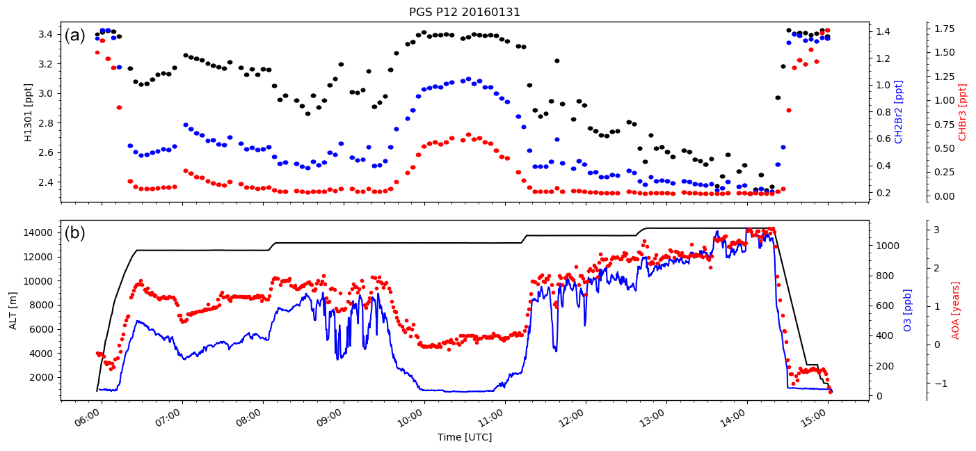
Figure 3Example of data gathered during a single flight of HALO during the PGS campaign. The flight PGS 12 started on 31 January 2016 from Kiruna in northern Sweden. Panel (a) shows measurements of the long-lived brominated source gas halon 1301 (CF3Br) and the short-lived source gases CH2Br2 and CHBr3, all measured with the GhOST-MS. Panel (b) shows flight altitude, ozone (parts per billion, ppb; 10−9; measured by the FAIRO instrument; Zahn et al., 2012) and mean age of air derived from SF6 measurements from the ECD channel of the GhOST-MS (1 min time resolution; see Bönisch et al., 2009, for a description of the measurement technique). An air mass with low ozone and also low mean age of air was observed during the middle of the flight between about 10:00 and 11:00 UTC. High mixing ratios of all three source gases are found in this region, as well as during take-off and landing of the aircraft. CHBr3 mixing ratios are close to detection limit when flying in aged stratospheric air masses, indicating a complete conversion of the bromine to its inorganic form.
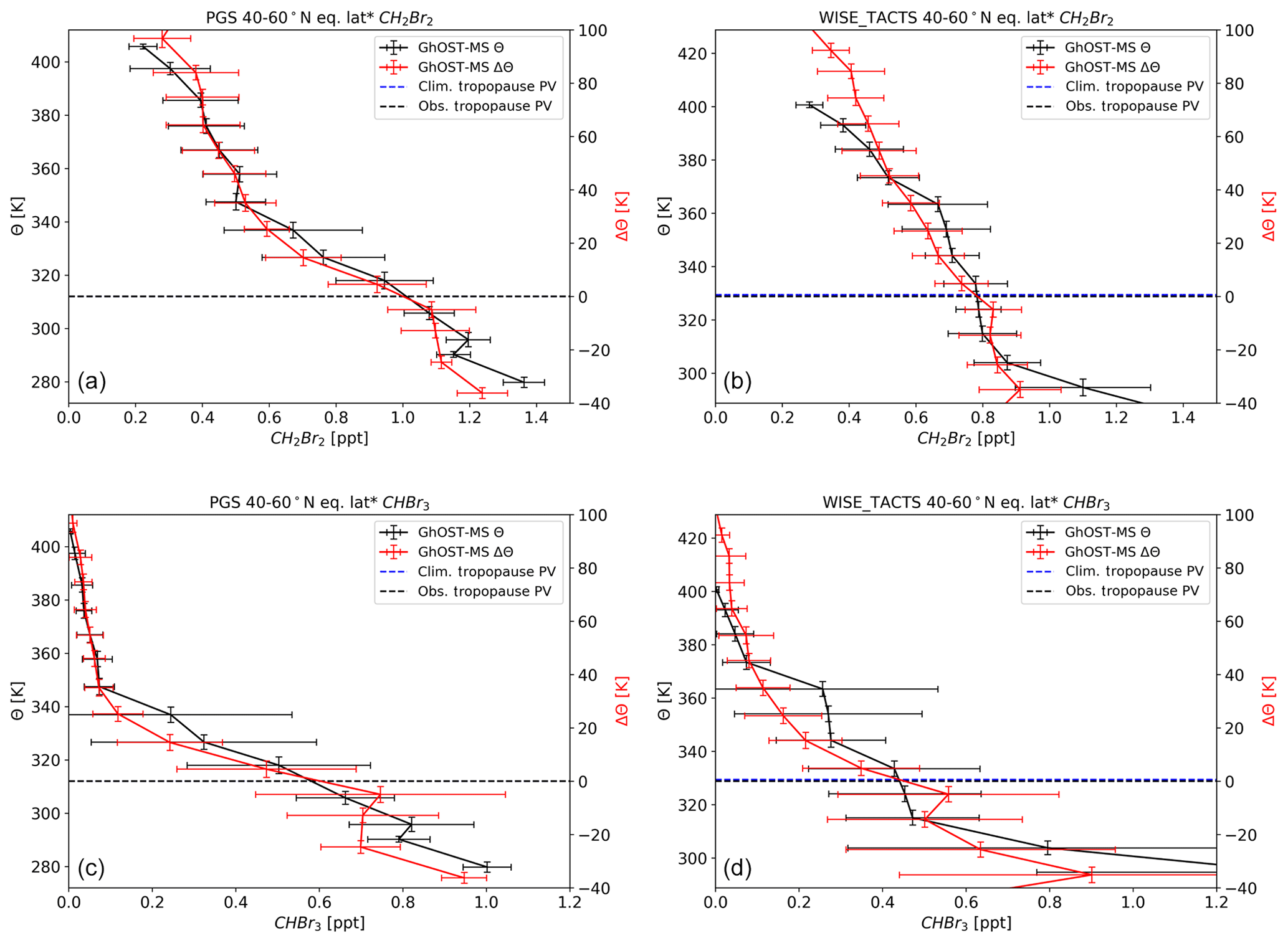
Figure 4Vertical profiles of CH2Br2 (a, b) and CHBr3 (c, d) averaged over 40–60∘ of equivalent latitude* and all flights during the PGS campaign (a, c, late December 2015 to March 2016) and from the merged dataset from the TACTS and WISE campaigns (b, d, representative of late summer to fall). The data are displayed as a function of potential temperature and potential temperature above the tropopause. The dashed blue line shows the zonal mean dynamical tropopause derived from ERA-Interim during September and October of the respective years in the Northern Hemisphere between 40 and 60∘ latitude, while the dashed black line is the average dynamical tropopause derived for the times and locations of our observations. Both vertical and horizontal error bars denote 1σ variability.
3.3 Upper tropospheric latitudinal gradients
If air is transported into the lowermost stratosphere via exchange with the extratropical upper troposphere, the levels of organic bromine compounds are likely to be different than for air being transported into the stratosphere via the tropical tropopause. In order to investigate the variability and the gradient in the upper tropospheric input region, we binned our data according to latitude and to potential temperature difference to the tropopause. All data in a range of 10 K below the local dynamical tropopause have been averaged to characterize the upper tropospheric input region. For these upper tropospheric data, standard latitude has been chosen and not equivalent latitude as for the stratospheric data. The latitudinal gradients are shown in Fig. 6 for CH2Br2, CHBr3 and total organic bromine derived from the sum of all VSLS (including the mixed bromochlorocarbons CH2BrCl, CHBrCl2 and CHBr2Cl), each weighted by the number of bromine atoms. For the tropical tropopause, input mixing ratios from different measurement campaigns have recently been reviewed by Engel and Rigby (2018). They found that total organic bromine from these five compounds averaged between 375 and 385 K; i.e. around the tropical tropopause it was 2.2 (0.8–4.2) ppt and in the upper tropical tropopause layer (TTL) (365–375 K potential temperature) it was around 2.8 (1.2–4.6) ppt. These upper TTL mixing ratios have also been included as reference in Fig. 6 (see also Table 5). The average mixing ratios derived here for the 10 K interval below the extratropical tropopause are larger. For data in the late summer to early fall from TACTS and WISE (Table 3), they increase from 2.6 ppt around 30∘ N (20–40∘ N equivalent latitude*) to 3.8 ppt around 50∘ N (40–60∘ N equivalent latitude*), while no further increase is found for higher latitudes with a total organic bromine mixing ratio of 3.4 ppt. For the winter measurements during PGS (Table 4), a clear increase with latitude is observed from 3.3 ppt around 30∘ N (20–40∘ N equivalent latitude*) via 3.8 ppt around 50∘ N (40–60∘ N equivalent latitude*) to 5.5 ppt in the high latitudes (60–80∘ N equivalent latitude*). There is considerable variability in these values derived in the upper troposphere, due to the short lifetime of these compounds and the high variability in emissions depending on the source region. Nevertheless, there is a clear tendency for an increase in tropopause mixing ratios with latitude, particularly during northern hemispheric winter. This is most probably related to the increase in lifetime with latitude, as especially during the wintertime PGS campaign the photolytical breakdown in higher latitudes is slower than in lower latitudes. Additional effects due to the sources and their latitudinal, seasonal and regional variability cannot be excluded. However, we note that emissions are most likely to be largest during summer, as shown in Hossaini et al. (2013), which would not explain the large mixing ratios of brominated VSLS in the upper troposphere in high latitudes during winter.
Table 5Mixing ratios of organic VSLS bromine in air at the tropical, and respectively extratropical (40–60∘ N), tropopause ( and ) used in the calculation of inorganic bromine (Bry) for the observation (OBS), and respectively the models, using the emission scenarios of Liang et al. (2010), Ordóñez et al. (2012), Ziska et al. (2013) and Warwick et al. (2006). For the Warwick et al. (2006) scenario, the data have been derived from the EMAC model, while for the other scenarios the TOMCAT model has been used. For the tropics, annual average for the years 2012 to 2016 have been calculated between 10∘ N and 10∘ S in a potential temperature range from 365 to 375 K. The tropical mixing ratios for the observations are from the observations compiled in the 2018 WMO report (Engel and Rigby, 2018) in the tropics between 365 and 375 K potential temperature. All data presented are shown in parts per trillion.
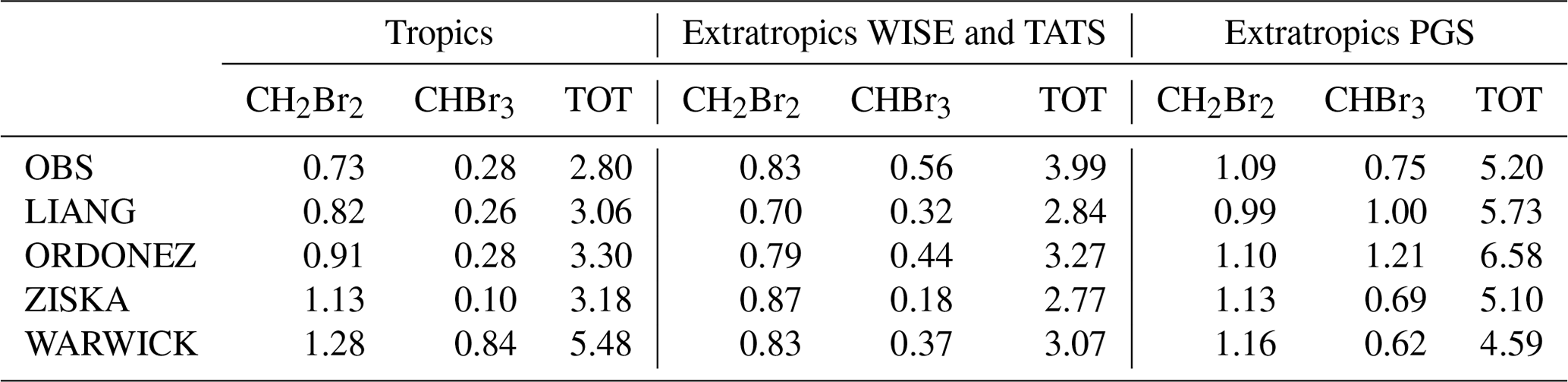

Figure 5Altitude–latitude cross sections of CH2Br2 (a, b) and CHBr3 (c, d) compiled from all flights during the PGS campaign from late December 2015 to March 2016 (a, c) and the TACTS WISE campaigns representative of conditions in late summer to early fall (b, d). The data are displayed as a function of θ* (see description in Sect. 2) and equivalent latitude*. The dynamical tropopause (dashed line) has been derived from the ERA-Interim reanalysis, providing a climatological mean zonal mean value of the tropopause.
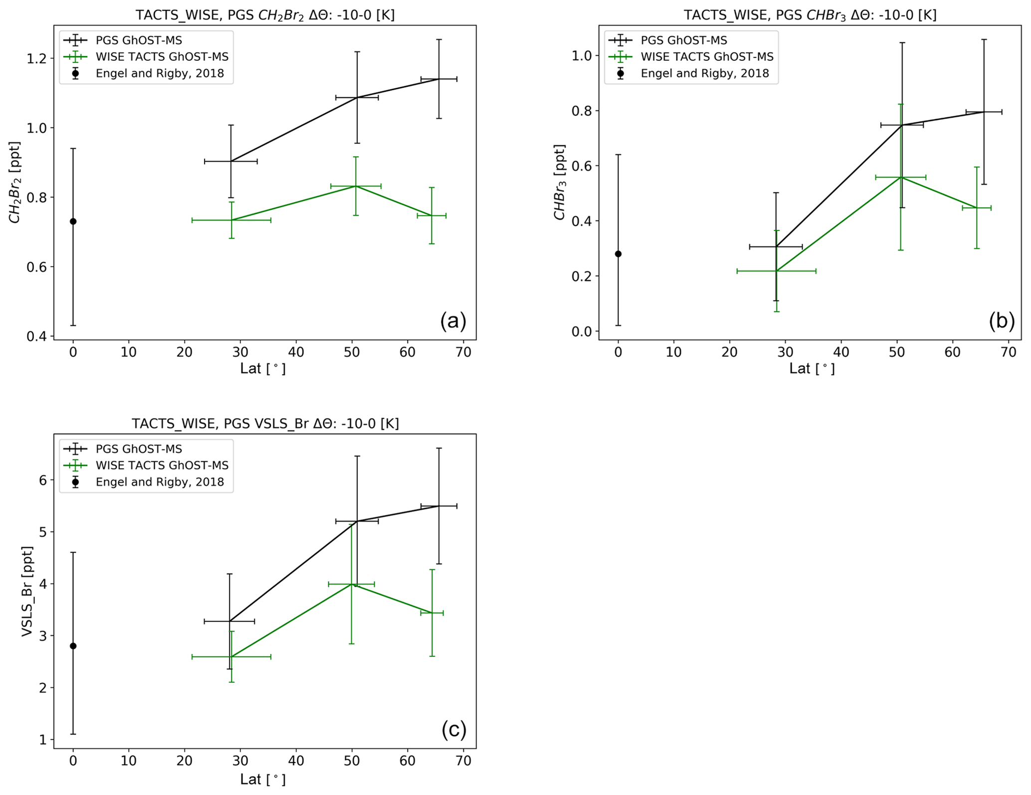
Figure 6Latitudinal cross section of CH2Br2 (a), CHBr3 (b) and total organic VSLS bromine (c) for all three campaigns, binned by latitude and averaged within 10 K below the local dynamical tropopause. Also included are the reference mixing ratios for the tropical tropopause (Engel and Rigby, 2018).
As bromocarbons are an important source of stratospheric bromine, it is worthwhile to investigate if current models can reproduce the observed distributions shown in Sect. 3. This is a prerequisite to realistically simulate the input of bromine from VSLS source gases to the stratosphere and also the further chemical breakdown and the transport processes related to the propagation of these gases in the stratosphere. As explained in Sect. 2, we used two different models with different emission scenarios for the brominated very-short-lived source gases. The ESCiMo simulation results from the chemistry climate model EMAC (Jöckel et al., 2016) are based on the emission scenario by Warwick et al. (2006), while the TOMCAT model (Hossaini et al., 2013) was run with three different emission scenarios (Ordóñez et al., 2012; Ziska et al., 2013; Liang et al., 2010). Both models have been used in the past to investigate the effect of brominated VSLS on the stratosphere (e.g. Sinnhuber and Meul, 2015; Hossaini et al., 2012, 2015; Wales et al., 2018; Graf, 2017). For the EMAC model, we have chosen to use results from a so-called “specified dynamics” simulation, which has been extended from the ESCiMo simulations to cover our campaign time period (see Sect. 2). The model data have been extracted for the time period and latitude ranges of the observations and have been zonally averaged. Here we compare vertical profiles, latitude–altitude cross sections and latitudinal gradients between our observations and the model results in a similar way as the observations have been presented in Sect. 3. We also compare results for total organic bromine. Only the scenarios of Warwick et al. (2006) and Ordóñez et al. (2012) contain emissions of the mixed bromochlorocarbons CH2BrCl, CHBrCl2 and CHBr2Cl. For the calculation of total VSLS organic bromine, based on the emission scenarios by Liang et al. (2010) and Ziska et al. (2013), we have adopted the results from the TOMCAT model using the emissions by Ordóñez et al. (2012). The contribution from these mixed bromochlorocarbons to total VSLS organic bromine is typically on the order of 20 %, while about 80 % of total VSLS organic bromine in the upper troposphere and lower stratosphere is due to CH2Br2 and CHBr3. This relative contribution of 20 % from minor VSLS is found in our observations (Tables 3 and 4) as well as in the values compiled in Engel and Rigby (2018) (see Table 5), and it is slightly larger than that derived, for example, in Fernandez et al. (2014).
4.1 Mean vertical profiles
Observed vertical profiles are available up to the maximum flight altitude of HALO, which is about 15 km, corresponding to about 400 K in potential temperature. Due to the variability of the tropopause potential temperature, this translates into a maximum of about 100 K for Δθ. The emphasis of this section is on the mid latitudes of the Northern Hemisphere, i.e. between 40 and 60∘ equivalent latitude*. All comparisons are shown as a function of Δθ. As no direct tropopause information was available for the TOMCAT output, we have chosen to derive Δθ for this comparison from the difference between model potential temperature and the potential temperature of the climatological zonal mean tropopause, which has been derived as explained in Sect. 2. As we are comparing our observations to the models in tropopause relative coordinates, we have also compared this climatological tropopause with the tropopause derived from the EMAC model results for the time of our campaigns. The potential temperature of the EMAC tropopause and the climatological tropopause differed by less than 3 K for all campaigns at mid latitudes.
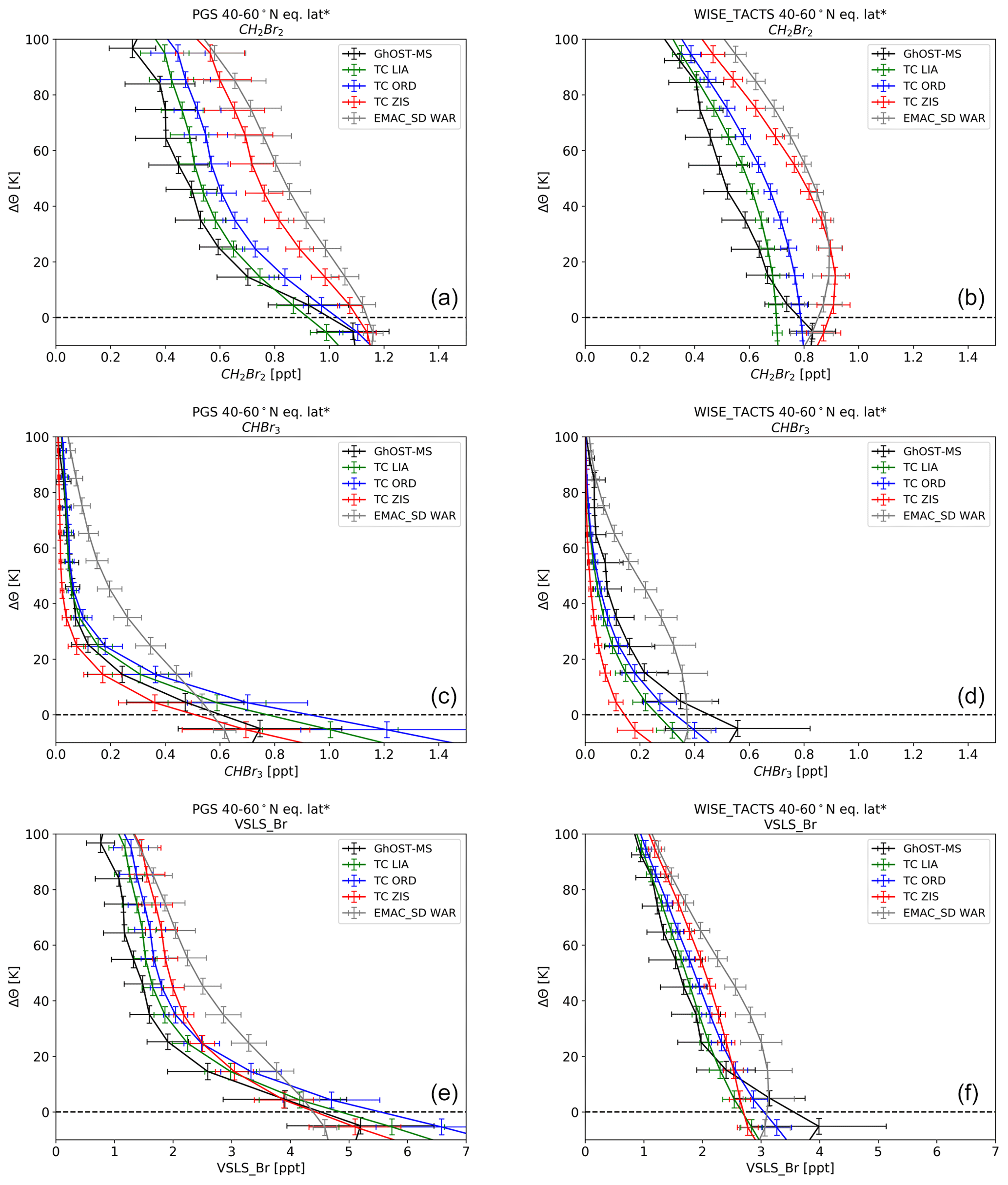
Figure 7Vertical profiles of CH2Br2 (a, b), CHBr3 (c, d) and total organic VSLS bromine (e, f) averaged over 40–60∘ of equivalent latitude* and all flights during the PGS campaign from late December 2015 to March 2016 (left-hand side) and from the combined WISE_TACTS dataset, representative of conditions in late summer to fall. Also shown are model results from the TOMCAT and EMAC model using different emission scenarios (see text for details). The data are displayed as a function of potential temperature above the dynamical tropopause. In the case when no model information on the tropopause altitude was available (TOMCAT), climatological tropopause values have been used (see text for details).
Figure 7 presents the model–measurement comparisons for the two main VSLS bromine source gases for the winter PGS campaign and for the combined dataset from WISE and TACTS. A similar figure for the minor VSLS is shown in the Supplement (Fig. S4). Overall the Liang et al. (2010) and the Ordoñez et al. (2012) emission scenarios give the best agreement with our observations of CH2Br2. The averaged deviation is 0.1 ppt or less, averaged over all campaigns and all stratospheric measurements in the 40–60∘ N equivalent latitude band, corresponding to a mean absolute percentage difference (MAPD) on the order of 10 %–25 %. Using the Ziska et al. (2013) emissions, CH2Br2 is overestimated in the mid-latitude lowest stratosphere during both campaigns by about 0.2 ppt, corresponding to about 40 %–60 % overestimation. The overestimation is even larger with 0.25–0.3 ppt (50 %–70 %) when using the Warwick et al. (2006) emissions in the EMAC model. As CHBr3 is nearly completely depleted in the upper part of the profiles, differences will become negligible there. Therefore, we only compared mixing ratios in the lowest 50 K potential temperature above the tropopause. In this region, the best agreement is again found with the Liang et al. (2010) and Ordoñez et al. (2012) emission scenarios, with mean differences always below 0.1 ppt, corresponding to a MAPD of about 20 %–30 %. Using the Ziska et al. (2013) emission scenario, we find an underestimation on the order of 0.05–0.1 ppt (40 %–70 %), while CHBr3 is overestimated by about 0.15 ppt (120 %–180 %) in the EMAC model based on the Warwick et al. (2006) emission scenario.
Using the Ziska et al. (2013) emission scenario, the overestimation of CH2Br2 and the underestimation of CHBr3 tend to cancel out. When adding the contribution from minor VSLS based on the scenario by Ordóñez et al. (2012), this results in a reasonable agreement in total VSLS organic bromine. The EMAC model with the Warwick et al. (2006) emissions substantially overestimates both CH2Br2 and CHBr3 in the lowermost stratosphere of the mid latitudes. The vertical profiles of CH2Br2 and CHBr3 from the EMAC model with the Warwick et al. (2006) emission scenario is therefore completely different from the observations, showing a maximum around the tropopause or even above.
We additionally compare model data from EMAC simulations using all four emission scenarios (Graf, 2017) in order to investigate if the large deviation of the Warwick et al. (2006) emission scenario is due to the EMAC model or due to the specific emission scenario. These simulations are only available for the time period up to 2011. This comparison for the January–March period (representative for the PGS campaign) is shown in Fig. 8 for CH2Br2 and CHBr3. Figure 8 looks qualitatively very similar to the comparisons in Fig. 7; i.e. both CH2Br2 and CHBr3 using the Warwick et al. (2006) emission scenario show highest mixing ratios in the lower stratosphere, and CHBr3 shows the least pronounced vertical gradients. Also, the pattern for the Ziska et al. (2013) emission scenario is the same, with the second highest CH2Br2 values and lowest CHBr3 values. Differences between the different models are certainly a factor in the explanation of model–observation differences. However, it is clear that the pattern when comparing all scenarios in the EMAC model is similar to that described above and that differences in the emission scenarios are the main driver of model–observation differences.
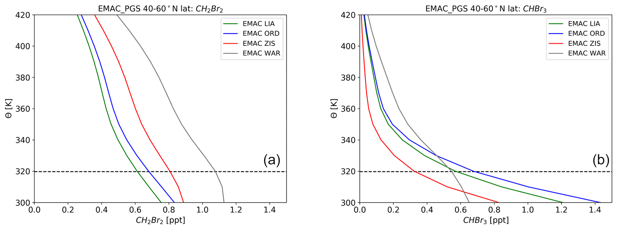
Figure 8Vertical profiles of CH2Br2 (a) and CHBr3 (b) averaged over 40–60∘ latitude from four model simulations with the EMAC model using the emission scenarios by Liang et al. (2010), Warwick et al. (2006), Ordóñez et al. (2012) and Ziska et al. (2013). The data have been averaged for the period from January to March, i.e. representative of the time period covered by the PGS campaign. The dashed line represents the model tropopause. Model results are nudged simulations of EMAC but do not cover the time period of our observations.
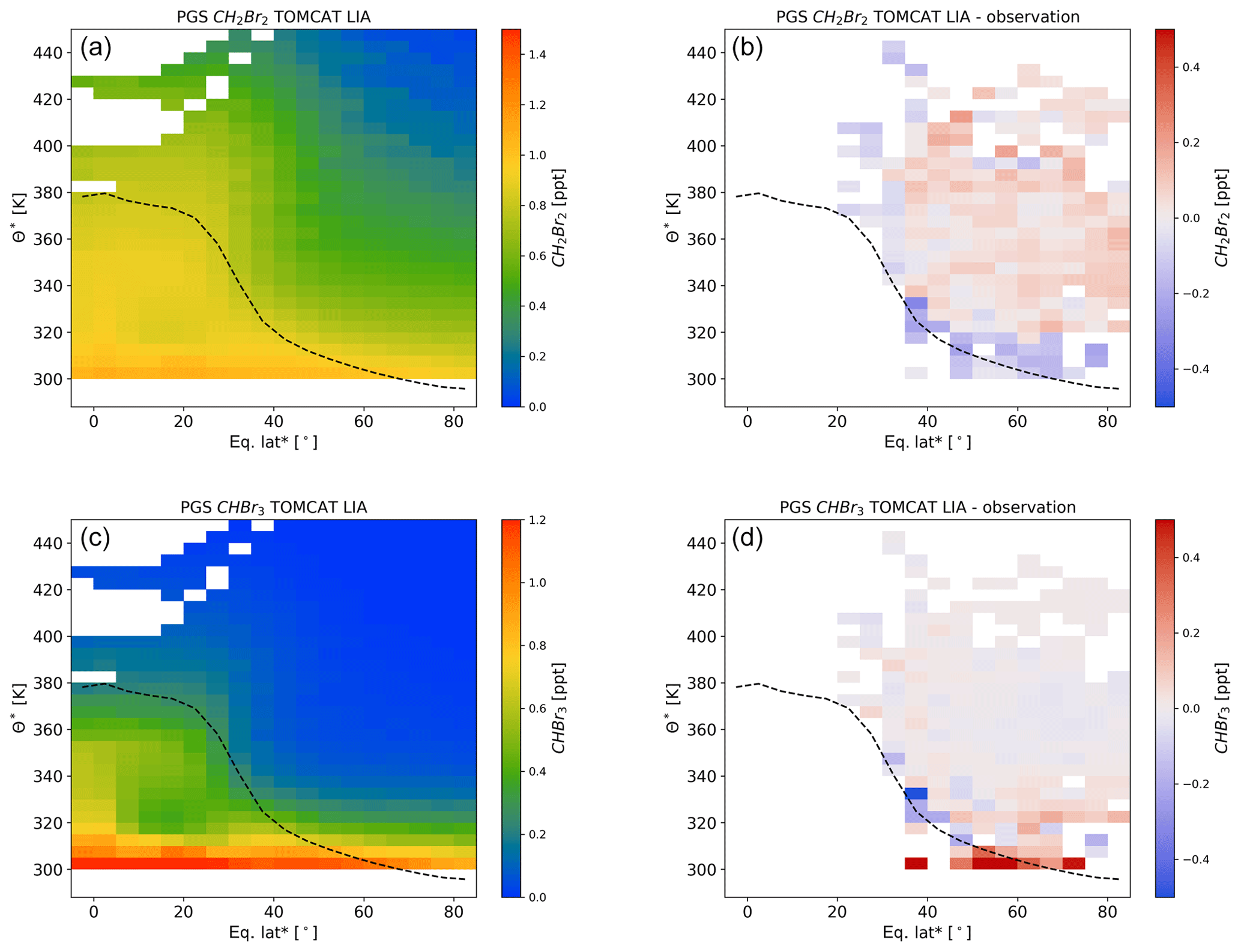
Figure 9Latitude–altitude cross section of CH2Br2 (a, b) and CHBr3 (c, d) for the TOMCAT model using the Liang et al. (2010) emission scenario (a, c) and differences to the observations (b, d) for all flights during the PGS campaign from late December 2015 to March 2016. The data are binned using equivalent latitude* and θ∗ as coordinates (see text for details). Also shown in the climatological mean tropopause (see text for details; dashed line). Boxes in which, due to the vertical resolution of the model, no values are available are left blank.
4.2 Latitude–altitude cross sections
As has been shown in the comparison of the vertical profiles, differences between model results and observations are found, especially in the case of the Ziska et al. (2013) emissions in the TOMCAT model and in the case of the Warwick et al. (2006) emissions in the EMAC model for the northern hemispheric mid latitudes (40–60∘ N). To visualize these differences, we present latitude–altitude cross sections of the model datasets and the differences to our observations in Figs. 9–12. While we use equivalent latitude* as the latitudinal coordinate for the observations and θ∗ as vertical coordinate, the zonal mean data are displayed as a function of latitude and potential temperature, θ, for the model results. The comparison is shown here for the winter dataset from PGS, for which the observational set covers a wide range of latitudes and also reaches very low tracer mole fractions. The comparison for the campaign in late summer to fall (TACTS and WISE) gives a rather similar picture (not shown). The overall best agreement in the vertical profiles has been found for the TOMCAT model using the emission scenarios by Liang et al. (2010) and Ordóñez et al. (2012). The latitude–altitude cross section for these two datasets is shown in Figs. 9 and 10. Using these two emission scenarios, the TOMCAT model tends to overestimate high-latitude tropospheric mole fractions of CHBr3 during this winter campaign. However, the stratospheric distribution is rather well reproduced with absolute deviations to the model mostly being below 0.1 ppt. In the case of CH2Br2, overall stratospheric mole fractions are slightly larger in the model results compared to the observations. The deviations between the TOMCAT model using the Ziska et al. (2010) emissions and the EMAC model using the Warwick et al. (2006) emissions are substantially larger. These are shown in Figs. 11 and 12 again for the PGS campaign. As noted above, the TOMCAT model with the Ziska et al. (2013) emissions overestimates stratospheric CH2Br2, while stratospheric CHBr3 is reasonably well captured. The largest discrepancies between model and observations are observed in the case of the EMAC model with the Warwick et al. (2006) emissions. In this case, both CH2Br2 and CHBr3 are overestimated in the lower stratosphere.
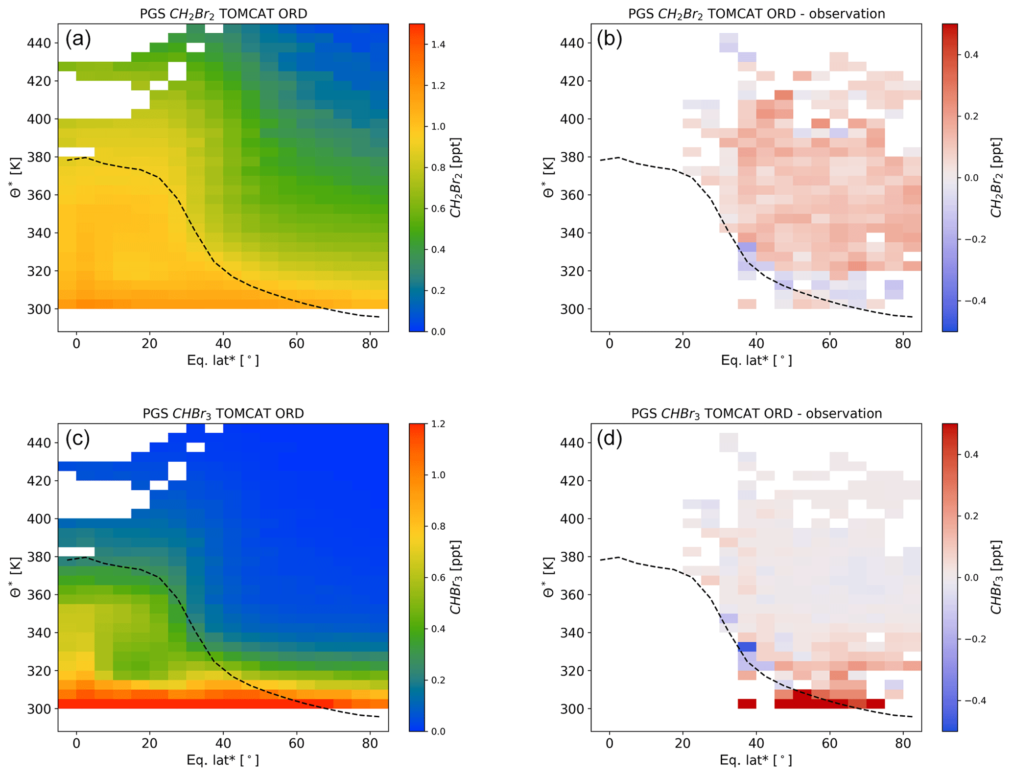
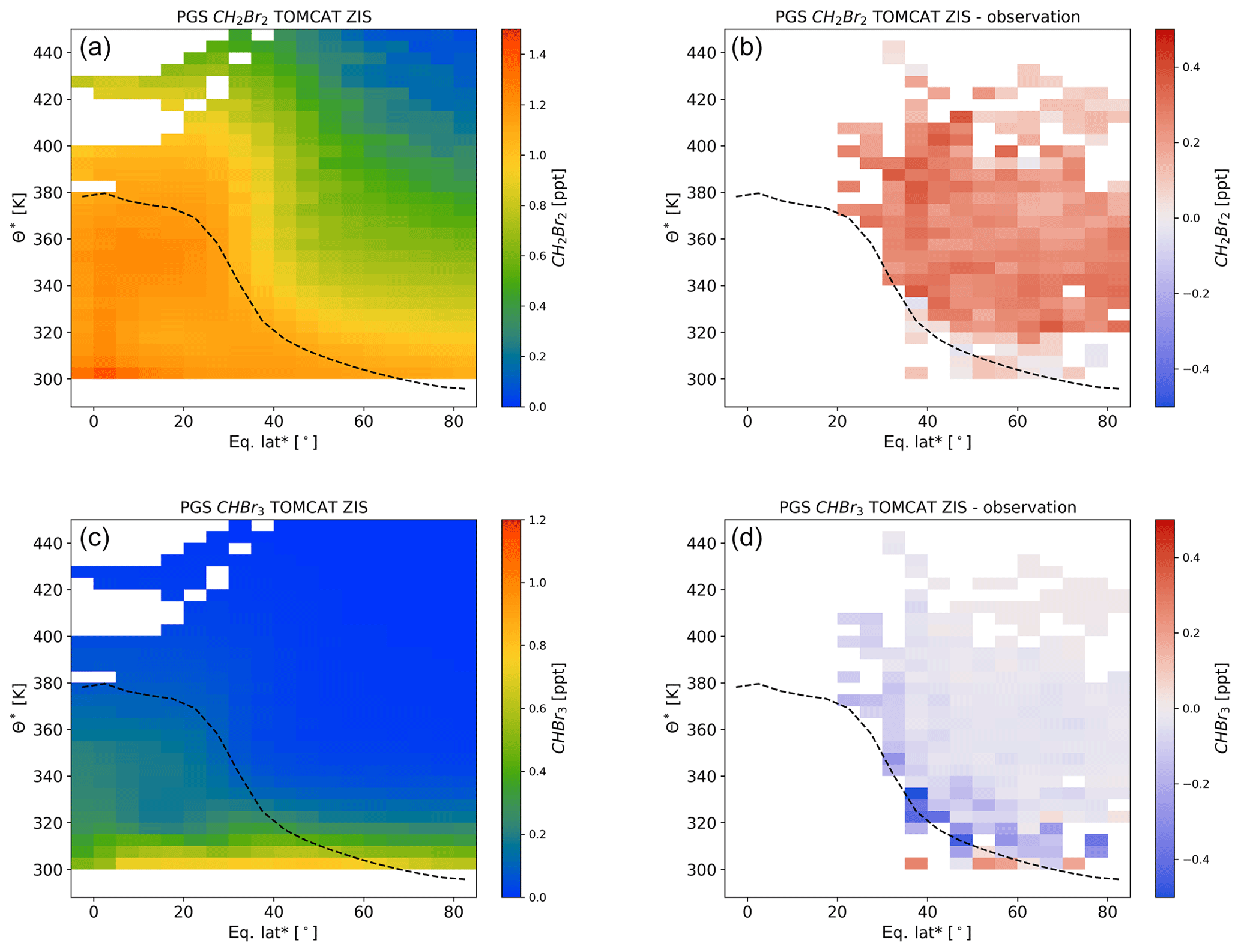
In the case of CHBr3, the two emission scenarios which have a more even distribution of emissions with latitude, i.e. the emission scenarios by Liang et al. (2010) and Ordoñez et al. (2012), show the best agreement with the observations. The emission scenario by Warwick et al. (2006) yields much higher mole fractions in the tropics and has the poorest agreement with measurement data. The emission scenario by Ziska et al. (2013) yields overall much lower CHBr3 in large parts of the atmosphere and seems to be the only set-up in which mid-latitude tropopause mixing ratios of CHBr3 are underestimated in comparison to our observations. For CH2Br2, again the Ordoñez et al. (2012) and Liang et al. (2010) emission scenarios in the TOMCAT model show rather similar distributions and rather good agreement with our observations. In the case of the TOMCAT model with the Ziska emissions, very high mole fractions of CH2Br2 are simulated throughout the tropics. Our low-latitude observations from HALO during late summer and fall (WISE and TACTS) and the values compiled in the WMO 2018 report for the tropics (Engel and Rigby, 2018) are lower by about 0.3–0.5 ppt than the mixing ratios of CH2Br2 in the tropics using the Warwick et al. (2006) and Ziska et al. (2013) emissions. The latitudinal distribution in the upper troposphere in models and observations is therefore investigated in more detail in the next section.
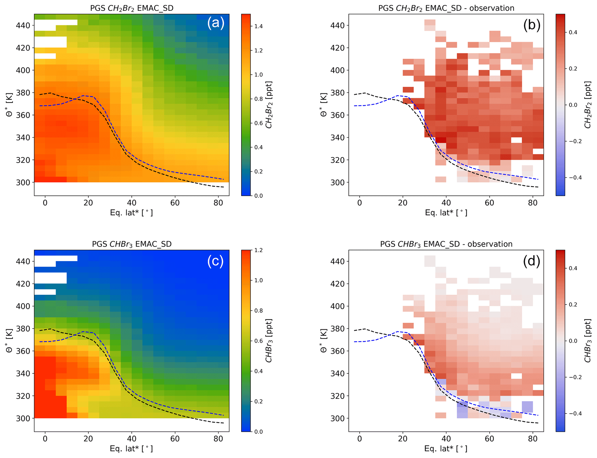
Figure 12As Figs. 9–11 but for the EMAC model using the Warwick et al. (2006) emission scenario.
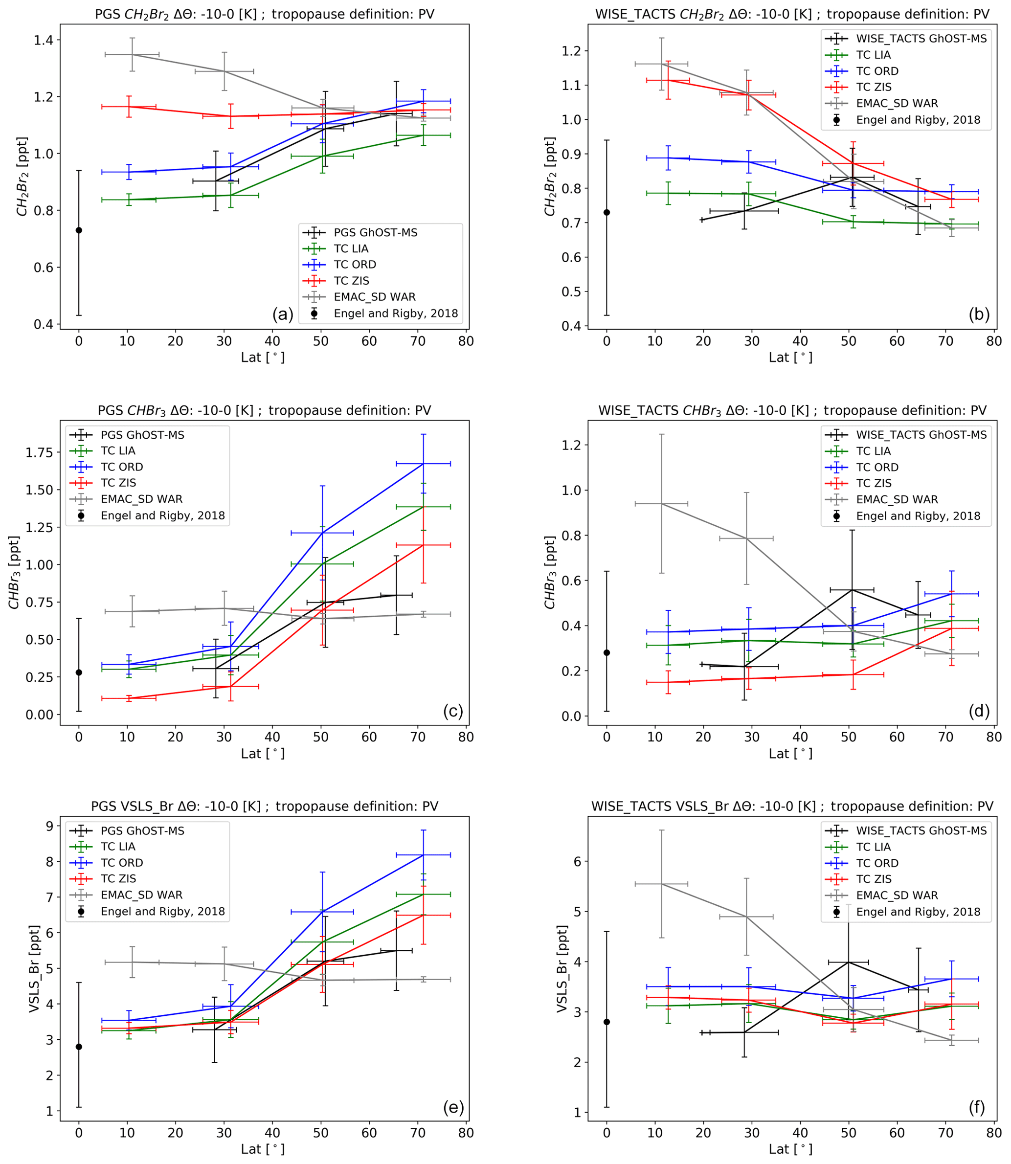
Figure 13Latitude cross section of tropopause representative mixing ratios of CH2Br2 (a, b) CHBr3 (c, d) and total organic VSLS bromine (a, b) for all the measurements from the PGS campaign (a, c, e) and WISE_TACTS dataset (b, d, f) from observations in comparison to all model emissions scenario combinations. Data are binned by latitude and averaged over 10 K below the tropopause. Due to the different sampling of the observations and the models, the centres of the different latitude bins are not the same for observations and models.
4.3 Upper tropospheric latitudinal gradients
Knowledge of the input of organic bromine into the stratosphere is crucial in understanding the stratospheric bromine budget and, therefore, also in determining the amount of inorganic bromine available for catalytic reactions involved in ozone depletion. For air masses in the stratosphere above about 400 K, it is generally assumed that the input is nearly exclusively through the tropical tropopause. For the lowermost stratosphere, however, input via the extratropical tropopause is also expected to play an important role (e.g. Holton et al., 1995; Gettelman et al., 2011). In order to investigate if the models are able to represent the latitudinal gradient in upper tropospheric mole fractions, we compare the observed extratropical mole fractions of the brominated VSLS in the upper troposphere (Sect. 3.3) and compiled tropical observations (Engel and Rigby, 2018) with those determined from the different model set-ups. For this purpose, the model data have been averaged in an interval of 10 K below the climatological (TOMCAT), or respectively modelled (EMAC), tropopause. The results are shown for the two main bromine VSLS, CH2Br2 and CHBr3, as well as for total VSLS organic bromine in Fig. 13 and Table 5 for the two campaign periods in comparison to observations. Note that for the scenarios by Liang et al. (2010) and Ziska et al. (2013), no estimates of emissions for the mixed bromochlorocarbons are available; instead, we have used the model results based on the Ordóñez et al. (2012) emissions for the calculation of total VSLS organic bromine.
During the two campaigns in late summer to fall (TACTS and WISE), all model set-ups show a decrease of CH2Br2 mixing ratios with latitude. Although, the latitudinal gradients are much steeper when the scenarios by Warwick et al. (2006) and Ziska et al. (2013) are used, which is due to overestimated mixing ratios at low latitudes. This is in good agreement with findings by Hossaini et al. (2013), who showed that TOMCAT using the Warwick et al. (2006) emission scenario overestimated HIAPER1 Pole-to-Pole Observations (HIPPO) in northern hemispheric mid latitudes. An increase in observed mixing ratios with latitude was found, especially during the winter PGS campaign, which is presumably related to the increase in atmospheric lifetime of compounds in the cold and dark high-latitude tropopause region during winter. This feature is qualitatively reproduced by the TOMCAT simulations with Liang et al. (2010) and Ordóñez et al. (2012) scenario, but not for the Ziska et al. (2013) and Warwick et al. (2006) scenario-based results, which show a moderate decrease and no latitudinal gradient. This feature is consistent with emissions in these two scenarios being more strongly biased towards the tropics.
For CHBr3, the observations show an increase with latitude, especially during the PGS campaign. The data in late summer to fall from TACTS and WISE show a less clear picture, with an increase between the subtropics and mid latitudes but a decrease towards high latitudes. This general tendency during the wintertime is reproduced by the TOMCAT model using all emission scenarios. Nonetheless, the gradient in the EMAC model results with the Warwick et al. (2006) emissions is reversed, which is mainly caused by the larger tropical mixing ratios and also evident from the latitude–altitude cross sections shown before. We also note that the subtropical mixing ratios based on the Ziska et al. (2013) emissions are lower than the observations.
The results for total organic bromine, including the three mixed bromochlorocarbons, can be mainly understood as a combination of the behaviour of CH2Br2 and CHBr3. In the case of the TOMCAT model with Ziska et al. (2013) emissions, a certain compensation is observed; i.e. total organic bromine is better reproduced than each compound by itself. This is due to an overestimation of CH2Br2, especially at low latitudes, and an underestimation of CHBr3. Total organic bromine from VSLS in the EMAC model using the Warwick et al. (2006) emissions is very different from the observations. It shows nearly constant mixing ratios with latitude during northern hemispheric winter (PGS) and a strong decrease during the period from late summer to fall of the TACTS and WISE campaigns. Most importantly, the overall levels, especially in the low latitudes, are much higher than our observations and also much higher than the tropical observations compiled in the WMO report (Engel and Rigby, 2018). We also note that poleward of 40∘ N and below 320 K (see Figs. 9 and 10) there is a small negative model bias for CH2Br2 at the extratropical tropopause when using the scenarios by Liang et al. (2010) and Ordóñez et al. (2012). At the same time the model simulations using these two scenarios yield a substantial positive bias for CHBr3 in the same region. This will result in a misrepresentation of the input of brominated VSLS source gases to the lowermost stratosphere via the different pathways.
As shown in the previous section, discrepancies exist between the various combinations of models and emission scenarios with respect to our observations, both around the tropopause and in the lower stratosphere. In this section, we will discuss the possible implications for inorganic bromine in the lower and lowermost stratosphere. Inorganic bromine is of key importance, as this is the form of bromine which can influence ozone through, for example, catalytic ozone depletion cycles. Note that this discussion only focuses on the input of bromine in the form of organic source gases (so-called source gas injection, SGI; see Engel and Rigby, 2018) from VSLS. The inorganic bromine from SGI can be derived as the difference between the organic bromine in the source region (tropopause) and the organic bromine still observed or modelled at a certain stratospheric location. The input of bromine into the stratosphere in the inorganic form (product gas injection) is expected to add more bromine in addition to the SGI discussed here. However, PGI cannot be investigated with the source gas measurements used in this study. Here, we focus on assessing what the different mixing ratios of bromine source gases at the tropical and extratropical tropopause in both observations and in model results imply for the total (organic and inorganic) bromine and inorganic bromine content of the lower and lowermost stratosphere.
We have shown in Sects. 3 and 4 that the organic bromine around the tropopause shows significant variability and also latitudinal gradients. In addition, large differences between the different model set-ups and observations are found. As mentioned in the introduction, the air in the extratropical lower and lowermost stratosphere is influenced by transport through the tropical and extratropical tropopause. As both regions show different levels or organic bromine source gases, the relative contribution of these source regions needs to be known to derive total bromine which entered the stratosphere and thus also inorganic bromine from SGI. Several authors have attempted to quantify the relative fractions of air masses from the different source regions based on tracer measurements (e.g. Hoor et al., 2005; Bönisch et al., 2009; Ray et al., 1999; Werner et al., 2010). No studies on mass fractions are available for the campaigns discussed here, so we will rely on previous studies for these fractions as discussed in the introduction to estimate the fractions of tropical and extratropical air in the lowermost stratosphere. The differences in Bry discussed here should thus be taken as a sensitivity study, and the values derived below can only be considered to be estimates showing how much the inorganic bromine may differ between different model set-ups and observations. In general, air masses close to the extratropical tropopause will be mainly of extratropical origin, while air masses near 400 K will almost be entirely of tropical origin. As a simplified approach, we have therefore chosen to assume that at the extratropical tropopause (Δθ=0), the extratropical fraction is 100 % and that this fraction decreases linearly to 0 % at 100 K above the tropopause. The organic bromine species transported into the stratosphere are chemically or photochemically depleted, and the bromine is transferred to the inorganic form. The total (organic and inorganic) bromine content from VSLS SGI in an air parcel in the lowermost stratosphere at Δθ above the tropopause, Brtot(Δθ), is thus the sum of organic, Brorg(Δθ), and inorganic, Brinorg (Δθ), bromine. Inorganic bromine is usually referred to as Bry.
The total bromine can also be described by summing up the organic bromine transported to the stratosphere via input through the tropical and extratropical tropopause.
where fex-trop and ftrop are the fractions of air of extratropical and of tropical origin, respectively, and and are the total organic VSLS bromine contents in air at the extratropical (40–60∘ N) and tropical tropopause, respectively, i.e. at Δθ=0. For observations only, the extratropical is available from our HALO campaigns. for the observations is therefore taken from observations at the tropical tropopause compiled in the 2018 WMO ozone assessment (Engel and Rigby, 2018). For the different model set-ups, and are derived from the global model fields. For the tropical input mixing ratios, the model output has been averaged between 10∘ S and 10∘ N in a potential temperature range from 365 to 375 K in a similar way as used for the observations (Engel and Rigby, 2018). Extratropical mixing ratios have been derived by averaging the model results, and respective observations, in a range of 10 K below the tropopause. In order to be consistent between models and observations, extratropical reference mixing ratios are derived for the time of the campaign, while the tropical tropopause mixing ratios are taken as seasonal mean.
Due to mass conservation, the sum of fex-trop and ftrop must be unity, so we can rewrite Eq. (2) to yield
If we assume that fex-trop increases linearly from 0 at Δθ=0 K to 1 at Δθ=100 K, the total bromine from VSLS SGI can be derived and the inorganic bromine, Bry(Δθ), is then calculated by combining Eqs. (1) and (3):
where Brorg(Δθ) is the organic bromine measured, and respectively simulated, at Δθ above the tropopause.
Figure 14 compares the vertical profiles of total and inorganic bromine derived in this way from the observations and the different model set-ups for the PGS campaign and the combined WISE_TACTS dataset. The values of and used for the models, and respectively the observations, are shown in Table 5.
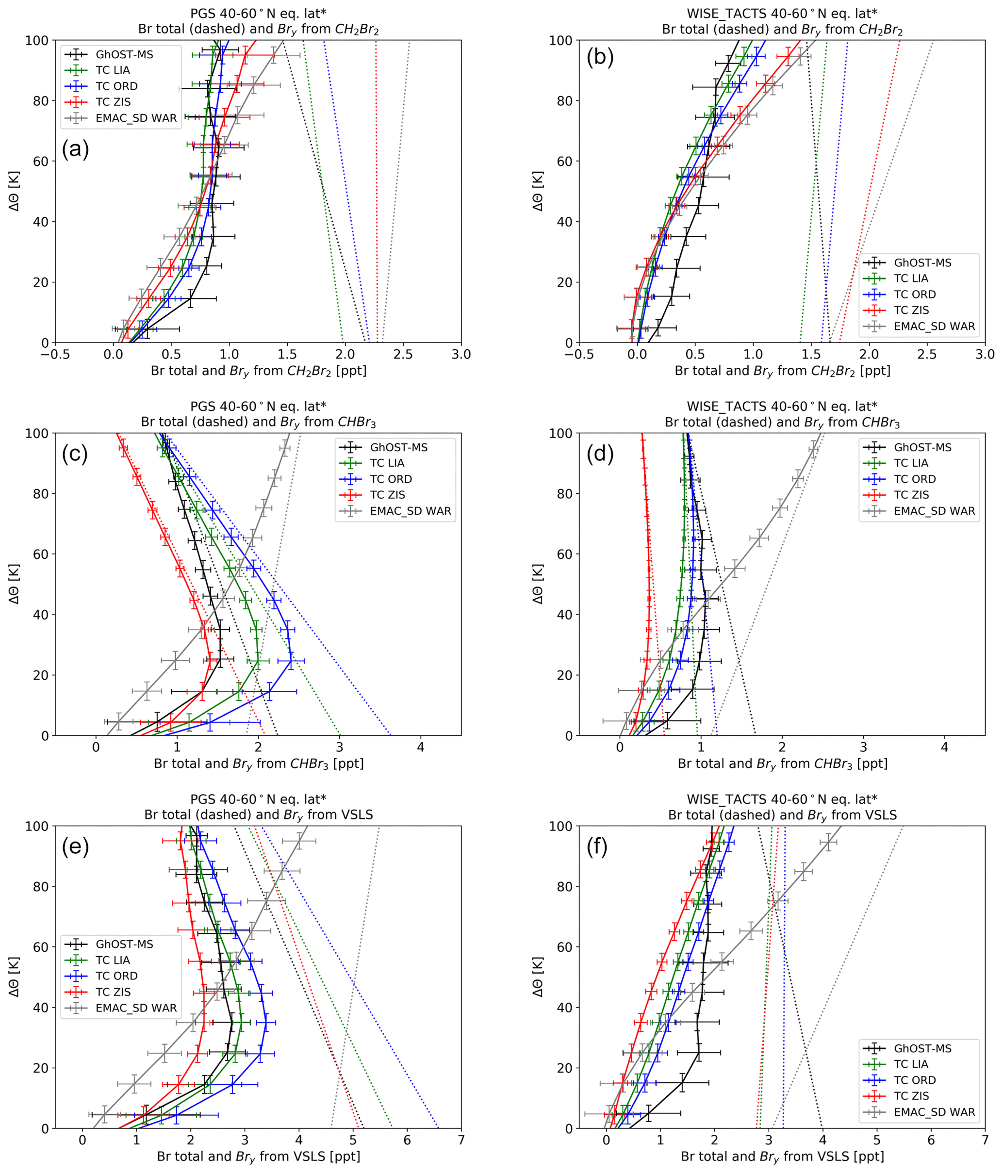
Figure 14Vertical profiles of Bry (solid lines) and total bromine (dotted lines) from CH2Br2, CHBr3 and total organic VSLS bromine averaged over 40–60∘ of equivalent latitude* for the winter PGS campaign (a, c, e, late December 2015 to March 2016) and the period form late summer to early fall (b, d, f, WISE and TACTS campaigns) in comparison to model results from the TOMCAT and the EMAC model using different emission scenarios (see text for details on calculation of Bry). Total bromine is calculated from data at the tropical and extratropical tropopause and using assumptions about fractional input from these two source regions (see text for details). The data are displayed as a function of potential temperature above the tropopause. In the case when no model information on the tropopause altitude was available (TOMCAT), climatological tropopause values have been used (see text for details).
Due to the nature of the set-up for the calculation of the SGI contribution to Bry described above, both model- and observation-derived Bry is close to zero at the extratropical tropopause. The assumed fractional contribution of tropical air increases with altitude, and thus the amount of organic bromine assumed at the tropical tropopause becomes more important in the calculation of total bromine and thus also in Bry. Overall, all model set-ups capture Bry from CH2Br2 rather well. For all campaigns, the Bry estimate from the observations is smaller than the model calculations above about 60 K above the tropopause and larger below this level. Under the given assumptions about fractional input, the larger Bry values derived in the model calculations above 60 K are caused by the higher total bromine values from CH2Br2, which are caused by the higher CH2Br2 levels at the tropical tropopause in comparison to the observations. For the campaigns in late summer to early fall, this difference is largest for the TOMCAT model with the Ziska et al. (2013) emissions and the EMAC model with the Warwick et al. (2006) emissions, consistent with these two model set-ups having the largest CH2Br2 mixing ratios at the tropical tropopause (1.13 and 1.28 ppt; see Table 5). Under the given assumptions about fractional input, the discrepancy in the lower part is more due to higher simulated CH2Br2 in the lowermost stratosphere than found in the observations. Using the emission scenarios by Liang et al. (2010) and Ordóñez et al. (2012), the differences are usually below 0.3 ppt of Bry, corresponding to a MAPD of less than 40 %.
Much larger variations are found in the amount of Bry derived from CHBr3. As can be seen from Fig. 7, the remaining organic bromine in the form of CHBr3 is very small for all three set-ups using the TOMCAT model and the observations already at about 30 to 40 K above the tropopause. The Bry from CHBr3 (solid lines in Fig. 14) is thus close to the total bromine in the form of CHBr3 (dotted lines in Fig. 14). In contrast, EMAC results using the Warwick et al. (2006) emissions still show substantial amounts of CHBr3 in the organic form even at 50 K above the tropopause and above. For the EMAC set-up, the Bry derived from CHBr3 is thus influenced by both the assumed input and the remaining organic CHBr3 in the stratosphere. However, the tropical input of CHBr3 in the EMAC model using the Warwick et al. (2006) emissions is very large (0.84 ppt, corresponding to about 2.5 ppt of bromine). Therefore, despite the fact that EMAC still shows substantial remaining CHBr3 rather deep into the lowermost stratosphere, this model set-up overestimates the amount of Bry due to CHBr3 in comparison to the observations. We find differences of about 1.5 ppt of Bry at about 100 K above the tropopause, which is about a factor of 3 higher than the mixing ratio derived from the observations. The amount of Bry from CHBr3 in the different emission scenarios used in TOMCAT is mainly determined by the amount of CHBr3 reaching the stratosphere, and especially for regions with Δθ above 50 K by the tropical input. As the TOMCAT model with the Ziska et al. (2013) emissions underestimates these tropical tropopause mixing ratios, it shows Bry amounts that are too small from CHBr3 throughout the stratosphere. In contrast, the tropical tropopause mixing ratio of CHBr3 from the Ordóñez et al. (2012) and Liang et al. (2010) scenarios are in better agreement with the observations presented here, and thus Bry estimates at 100 K above the tropopause are in good agreement with the observation-based estimates.

Figure 15Sensitivity of Bry from CH2Br2 and CHBr3 at Δθ=40 K as a function of the fraction of extratropical air for the PGS campaign from January to April 2016 for observations in comparison to the different model calculations.
The total Bry from VSLS SGI can be understood mainly as an addition of the contributions of CH2Br2 and CHBr3, as these are responsible for about 80 % of total VSLS organic bromine. As the differences are largest for CHBr3, this dominates the differences in total Bry from VSLS SGI. Interestingly, while the Ziska et al. (2013) emissions in TOMCAT showed some significant differences, in particular for CHBr3 at the tropopause, the differences in total Bry are not as large. The underestimation of Bry from CHBr3 is partly compensated by an overestimation of Bry from CH2Br2. The EMAC model with the Warwick et al. (2006) emissions overestimates Bry from both CH2Br2 and CHBr3, so that in total a difference in Bry of more than 2 ppt is derived, corresponding to an overestimation by a factor of more than 2 with respect to observation-derived values. This difference is expected to have a significant effect on ozone chemistry in the lower stratosphere.
The Bry mixing ratios derived in the approach described above depend on the assumed input mixing ratios but also on the assumed fractional contribution of air from the tropics and the extratropics. In order to test the sensitivity of the results on the assumed fractions, we have varied the fractional input. Figure 15 shows the Bry, derived from CH2Br2 and CHBr3 for the PGS campaign at 40 K above the tropopause, as a function of the assumed fractional contribution from the extratropical source region (fex-trop); the tropical fraction ftrop is then always (1−fex-trop). A similar figure (Fig. S5) is shown for the WISE_TACTS dataset in the Supplement. While the differences are not very large for CH2Br2, which shows a much less pronounced latitudinal gradient, differences for CHBr3 can be very large. This is particularly true for the EMAC model with the Warwick et al. (2006) scenario, where the dependency of Bry on the fractional input behaves in an opposite way to the CHBr3 observations and the other model-emission scenario combinations. This shows that for the calculation of Bry in the lowermost stratosphere from observations, it is necessary to have a good knowledge of the relative contributions and that for models it is necessary to have a realistic representation not only of chemistry but also of transport in the lowermost stratosphere.
We present a large dataset of around 4000 in situ measurements of five brominated VSLS with the GhOST-MS instrument in the UTLS region using HALO. We used data from the three HALO missions: TACTS, WISE and PGS. Data are presented in tropopause-relative coordinates, i.e. the difference in potential temperature relative to the dynamical tropopause, defined by the value of 2 PVU. Stratospheric data are sorted by equivalent latitude, while we used normal latitude for tropospheric data. We find systematic variabilities with latitude, altitude and season. The shortest-lived VSLS mixing ratios decrease fastest with altitude. During polar winter, vertical gradients are larger than during late summer to early fall, which is in line with the well-known diabatic descent of stratospheric air during polar winter. An important aspect of the observed distributions is that CHBr3 mixing ratios at the extratropical tropopause are systematically higher than those at the tropical tropopause. A similar feature is found for CH2Br2, although the latitudinal gradient is less pronounced than in the case of CHBr3. The increase of VSLS mole fractions is especially clear during northern hemispheric winter, when lifetimes become very long at high latitudes.
We further compared the observed distributions with a range of modelled distributions from TOMCAT and EMAC, run with different global emission scenarios. The features of the observed distribution are partly reproduced by the model calculations, with large differences caused by the different emissions. Overall, for CH2Br2, we find much better agreement between observations and model output for simulations using the emission scenarios by Liang et al. (2010) and Ordóñez et al. (2012), which have lower overall emissions than the scenarios by Ziska et al. (2013) and Warwick et al. (2006). This is in agreement with a recently proposed revision of the best estimate of global CH2Br2 emissions towards the lower edge of previous estimates (Engel and Rigby, 2018) . In the case of CHBr3, the use of the emission scenario by Ziska et al. (2013), which has the lowest global emissions, results in mixing ratios that are too low at the tropical tropopause and also at the extratropical tropopause. The use of the emission scenario by Warwick et al. (2006) results in strongly elevated mixing ratios of CHBr3 at the tropical tropopause and a reversed latitudinal gradient at the tropopause in comparison to the observations. These findings are in good agreement with previous comparisons of the different emission scenarios (Hossaini et al., 2013, 2016) for CH2Br2. For CHBr3, Hossaini et al. (2016) found that the lower emissions in the Ziska et al. (2013) scenario generally gave best agreement with ground-based observations in the tropics. However, the tropopause mixing ratios derived with this scenario are too low, both in the tropics and in the extratropics. In a recent paper, Fiehn et al. (2018) discussed that a modified version of the Ziska et al. (2013) scenario, with seasonally varying emissions, yielded significantly higher tropopause values. The Ordóñez et al. (2012) scenario, which has higher emissions than the Ziska et al. (2013) scenario, yielded mixing ratios of CHBr3 that are too high during the winter period. It is clear that no scenario is able to capture tropical and extratropical values from our observations. However, it is clear from the comparison with the scenario by Warwick et al. (2006), which restricts emissions to latitudes below 50∘, that the sources of these short-lived brominated compounds are not only in the tropics, because significant emissions must also occur at higher latitudes. This is consistent with comparison of tropospheric data (see Fig. 6 in Hossaini et al., 2013). For improved emission scenarios, more emphasis on the seasonality of the sources might also lead to an improvement.
Air in the lowermost stratosphere is composed of air masses originating from both the tropical and the extratropical upper troposphere. The latitudinal gradient of VSLS will therefore impact the amount of bromine transported into the stratosphere and thus also the amount of reactive, inorganic bromine (Bry) in the lowermost stratosphere able to contribute to catalytic ozone depletion. The bromine budget in the lower stratosphere will depend on the relative fraction of air from the tropical and extratropical tropopause. The relative contribution of extratropical air decreases with latitude and reaches zero at about 400 K potential temperature. Using simplified assumptions about the fractional distributions, we derive substantial differences in stratospheric Bry, depending on the emission scenario. These can be as high as 2 ppt, corresponding to a difference of a factor of 2 relative to observation-derived values, when using the scenario by Warwick et al. (2006). Typical differences in Bry when using the other scenarios are on the order of 1 ppt. This is expected to have an impact on modelled ozone depletion in the lower stratosphere. For example, it has been shown that inclusion of about 5 ppt of Bry from VSLS leads to an expansion of the ozone hole area of km2 and an increase in maximum Antarctic ozone hole depletion by up to 14 % (Fernandez et al., 2017). The impact of bromine on ozone is most pronounced in the lowest part of the stratosphere (Hossaini et al., 2015). Further, as the efficiency of bromine to destroy ozone depends on the amount of available chlorine, it is also likely that modelled temporal trends of ozone will be influenced, even if there are no long-term changes in VSLS bromine. If relative contributions of the different pathways (tropical vs. extratropical air) change, e.g. due to changes in stratospheric circulation, this could further influence ozone due to the different amounts of bromine in these air masses. As shown in our sensitivity study (Sect. 5), the assumptions on the relative contribution of the different source regions has a substantial impact especially on the Bry produced from CHBr3 in the lowermost stratosphere.
While the dataset presented here provides a much better picture of the distribution of brominated VSLS in the UTLS region than previously available, there are still considerable gaps in our knowledge of the distribution of these species. Only data in late summer to fall and winter have been presented here for the Northern Hemisphere. Spring and early summer are less well covered, as is the Southern Hemisphere. Southern hemispheric distributions are expected to differ from northern hemispheric distributions, as the main sources of many brominated VSLS are believed to be from coastal ocean regions. Due to the different distribution of oceans, land and coastal areas between the hemispheres, it is not possible to extrapolate northern hemispheric observations to the Southern Hemisphere. Further, while no signs of increasing emissions of natural brominated VSLS have been observed so far, such an increase is possible in a changing climate and needs to be monitored.
The observational data are available via the HALO Database (halo-db.pa.op.dlr.de/). The data of the ESCiMo simulations using the EMAC model will be made available in the Climate and Environmental Retrieval and Archive (CERA) database at the German Climate Computing Centre (DKRZ; https://cera-www.dkrz.de, Jöckel et al., 2016); the simulations results of Graf (2017) are available upon request. TOMCAT model data will be uploaded to the Lancaster University data repository upon article acceptance. Access to data may be dependent on the signature of a data protocol.
The supplement related to this article is available online at: https://doi.org/10.5194/acp-20-4105-2020-supplement.
TK, FO, HB and AE were involved in developing the GhOST instrument and operating it in the field during the missions, data evaluation and interpretation. FL, MH and TS were also involved in the operation, evaluation and interpretation. NS, AR and CH were involved in the evaluation and interpretation. RH, PG and PJ have provided model data and also participated in the discussion of the data and the comparisons. AE and TK have mainly written the article. All co-authors were involved in the discussion and iterations of the article.
The authors declare that they have no conflict of interest.
The work carried out at the University Frankfurt has been funded through several projects by the German Science Foundation (DFG) for the development and operation of GHOST-MS and for the measurement campaigns (EN367/5, EN367/8, EN367/11, EN367/13 and EN367/14). Andreas Engel would like to thank CSIRO in Aspendale, Australia, for a Frohlich Fellowship, during which parts of this analysis was performed. Many thanks also to Kieran Stanley for proof reading and improving the article. We would further like to thank the DLR staff, including pilots and ground staff, for the operation of HALO and the support during the campaigns. The good collaboration with the other groups involved in the HALO campaigns is also acknowledged. We would like to thank Andreas Zahn from KIT Karlsruhe for provision of the ozone data in Fig. 3. We further thank Jens-Uwe Grooß from Forschungszentrum Jülich for the calculation of the tropopause and equivalent latitude for the HALO campaigns and Michael Sprenger from ETH Zürich for the provision of the climatological dynamical tropopause from ERA-Interim data. Ryan Hossaini is supported by a NERC Independent Research Fellowship (NE/N014375/1). The EMAC simulations have been performed at the German Climate Computing Centre (DKRZ) through support from the Bundesministerium für Bildung und Forschung (BMBF). DKRZ and its scientific steering committee are gratefully acknowledged for providing the high-performance computing and data archiving resources for this consortial project (ESCiMo: Earth System Chemistry integrated Modelling).
This research has been supported by the Deutsche Forschungsgemeinschaft (DFG) (grant nos. EN367/5, EN367/8, EN367/11, EN367/13 and EN367/14).
This paper was edited by Farahnaz Khosrawi and reviewed by Rafael Pedro Fernandez, Stefanie Falk, and one anonymous referee.
Appenzeller, C., Holton, J. R., and Rosenlof, K. H.: Seasonal variation of mass transport across the tropopause, J. Geophys. Res.-Atmos., 101, 15071–15078, 1996.
Ball, W. T., Alsing, J., Mortlock, D. J., Staehelin, J., Haigh, J. D., Peter, T., Tummon, F., Stübi, R., Stenke, A., Anderson, J., Bourassa, A., Davis, S. M., Degenstein, D., Frith, S., Froidevaux, L., Roth, C., Sofieva, V., Wang, R., Wild, J., Yu, P., Ziemke, J. R., and Rozanov, E. V.: Evidence for a continuous decline in lower stratospheric ozone offsetting ozone layer recovery, Atmos. Chem. Phys., 18, 1379–1394, https://doi.org/10.5194/acp-18-1379-2018, 2018.
Bönisch, H., Hoor, P., Gurk, C., Feng, W., Chipperfield, M., Engel, A., and Bregman, B.: Model evaluation of CO2 and SF6 in the extratropical UT/LS region, J. Geophys. Res.-Atmos., 113, D06101, https://doi.org/10.1029/2007jd008829, 2008.
Bönisch, H., Engel, A., Curtius, J., Birner, Th., and Hoor, P.: Quantifying transport into the lowermost stratosphere using simultaneous in-situ measurements of SF6 and CO2, Atmos. Chem. Phys., 9, 5905–5919, https://doi.org/10.5194/acp-9-5905-2009, 2009.
Bönisch, H., Engel, A., Birner, T., Hoor, P., Tarasick, D. W., and Ray, E. A.: On the structural changes in the Brewer-Dobson circulation after 2000, Atmos. Chem. Phys., 11, 3937–3948, https://doi.org/10.5194/acp-11-3937-2011, 2011.
Boothe, A. C. and Homeyer, C. R.: Global large-scale stratosphere–troposphere exchange in modern reanalyses, Atmos. Chem. Phys., 17, 5537–5559, https://doi.org/10.5194/acp-17-5537-2017, 2017.
Burkholder, J. B.: (Lead Author) Hodnebrog, Ø., and Orkin, V. L.: Summary of Abundances, Lifetimes, Ozone Depletion Potentials (ODPs), Radiative Efficiencies (REs), Global Warming Potentials (GWPs), and Global Temperature change Potentials (GTPs) Appendix 1 to Scientific Assessment of Ozone Depletion: 2018, Global Ozone Research and Monitoring Project-Report No. 58, World Meteorological Organization, Geneva, Switzerland, 2018.
Burkholder, J. B., Sander, S. P., Abbatt, J., Barker, J. R., Huie, R. E., Kolb, C. E., Kurylo, M. J., Orkin, V. L., Wilmouth, D. M., and Wine, P. H. C. K. A. P. D. F. U. I. A. S.: Chemical kinetics and photochemical data for use in atmospheric studies, Evaluation number 18, JPL Publication 15-10, Jet Propulsion Laboratory, 2015.
Carpenter, L. J., Reimann, S., Burkholder, J. B., Clerbaux, C., Hall, B. D., Hossaini, R., Laube, J. C., and Yvon-Lewis, S. A.: Ozone-Depleting Substances (ODSs) and Other Gases of Interest to the Montreal Protocol, Chapter 1 in Scientific Assessment of Ozone Depletion: 2014, Global Ozone Research and Monitoring Project – Report No. 55, World Meteorological Organization, Geneva, Switzerland, 2014.
Chipperfield, M. P.: New version of the TOMCAT/SLIMCAT off-line chemical transport model: Intercomparison of stratospheric tracer experiments, Q. J. Roy. Meteor. Soc., 132, 1179–1203, https://doi.org/10.1256/qj.05.51, 2006.
Chipperfield, M. P., Dhomse, S., Hossaini, R., Feng, W., Santee, M. L., Weber, M., Burrows, J. P., Wild, J. D., Loyola, D., and Coldewey-Egbers, M.: On the Cause of Recent Variations in Lower Stratospheric Ozone, Geophys. Res. Lett., 45, 5718–5726, https://doi.org/10.1029/2018GL078071, 2018.
Daniel, J. S., and Velders, G. J. M., Douglass, A. R., Forster, P. M. D., Hauglustaine, D. A., Isaksen, I. S. A., Kuijpers, L. J. M., Mc-Culloch, A., and Wallington, T.: JHalocarbon scenarios, ozonedepletion potentials, and global warming potentials, chap. 8, in: World Meteorological Organization: Scientific assessment ofozone depletion: 2006, Global Ozone Research and MonitoringProject – Report No. 50, Geneva, 2006.
Dee, D. P., Uppala, S. M., Simmons, A. J., Berrisford, P., Poli, P., Kobayashi, S., Andrae, U., Balmaseda, M. A., Balsamo, G., Bauer, P., Bechtold, P., Beljaars, A. C. M., van de Berg, L., Bidlot, J., Bormann, N., Delsol, C., Dragani, R., Fuentes, M., Geer, A. J., Haimberger, L., Healy, S. B., Hersbach, H., Hólm, E. V., Isaksen, L., Kållberg, P., Köhler, M., Matricardi, M., McNally, A. P., Monge-Sanz, B. M., Morcrette, J.-J., Park, B.-K., Peubey, C., de Rosnay, P., Tavolato, C., Thépaut, J.-N., and Vitart, F.: The ERA-Interim reanalysis: configuration and performance of the data assimilation system, Q. J. Roy. Meteor. Soc., 137, 553–597, https://doi.org/10.1002/qj.828, 2011.
Dhomse, S. S., Chipperfield, M. P., Feng, W., Hossaini, R., Mann, G. W., and Santee, M. L.: Revisiting the hemispheric asymmetry in midlatitude ozone changes following the Mount Pinatubo eruption: A 3-D model study, Geophys. Res. Lett., 42, 3038–3047, https://doi.org/10.1002/2015gl063052, 2015.
Engel, A. and Rigby, M., Burkholder, J. B., Fernandez, R. P., Froidevaux, L., Hall, B. D., Hossaini, R., Saito, T., Vollmer, M. K., and Yao, B.: Update on Ozone-Depleting Substances (ODS) and Other Gases of Interest to the Montreal Protocol, chap. 1, in: Scientific Assessment of Ozone Depletion: 2018, Global Ozone Research and Monitoring Project-Report No. 58, World Meteorological Organization, Geneva, Switzerland, 2018.
Engel, A., Bönisch, H., Brunner, D., Fischer, H., Franke, H., Günther, G., Gurk, C., Hegglin, M., Hoor, P., Königstedt, R., Krebsbach, M., Maser, R., Parchatka, U., Peter, T., Schell, D., Schiller, C., Schmidt, U., Spelten, N., Szabo, T., Weers, U., Wernli, H., Wetter, T., and Wirth, V.: Highly resolved observations of trace gases in the lowermost stratosphere and upper troposphere from the Spurt project: an overview, Atmos. Chem. Phys., 6, 283–301, https://doi.org/10.5194/acp-6-283-2006, 2006.
Falk, S., Sinnhuber, B. M., Krysztofiak, G., Jöckel, P., Graf, P., and Lennartz, S. T.: Brominated VSLS and their influence on ozone under a changing climate, Atmos. Chem. Phys., 17, 11313–11329, https://doi.org/10.5194/acp-17-11313-2017, 2017.
Farman, J. C., Gardiner, B. G., and Shanklin, J. D.: Large Losses of Total Ozone in Antarctica Reveal Seasonal Clox/Nox Interaction, Nature, 315, 207–210, https://doi.org/10.1038/315207a0, 1985.
Feng, W., Chipperfield, M. P., Dorf, M., Pfeilsticker, K., and Ricaud, P.: Mid-latitude ozone changes: studies with a 3-D CTM forced by ERA-40 analyses, Atmos. Chem. Phys., 7, 2357–2369, https://doi.org/10.5194/acp-7-2357-2007, 2007.
Fernandez, R. P., Salawitch, R. J., Kinnison, D. E., Lamarque, J. F., and Saiz-Lopez, A.: Bromine partitioning in the tropical tropopause layer: implications for stratospheric injection, Atmos. Chem. Phys., 14, 13391–13410, https://doi.org/10.5194/acp-14-13391-2014, 2014.
Fernandez, R. P., Kinnison, D. E., Lamarque, J.-F., Tilmes, S., and Saiz-Lopez, A.: Impact of biogenic very short-lived bromine on the Antarctic ozone hole during the 21st century, Atmos. Chem. Phys., 17, 1673–1688, https://doi.org/10.5194/acp-17-1673-2017, 2017.
Fiehn, A., Quack, B., Hepach, H., Fuhlbrügge, S., Tegtmeier, S., Toohey, M., Atlas, E., and Krüger, K.: Delivery of halogenated very short-lived substances from the west Indian Ocean to the stratosphere during the Asian summer monsoon, Atmos. Chem. Phys., 17, 6723–6741, https://doi.org/10.5194/acp-17-6723-2017, 2017.
Fiehn, A., Quack, B., Stemmler, I., Ziska, F., and Krüger, K.: Importance of seasonally resolved oceanic emissions for bromoform delivery from the tropical Indian Ocean and west Pacific to the stratosphere, Atmos. Chem. Phys., 18, 11973–11990, https://doi.org/10.5194/acp-18-11973-2018, 2018.
Fischer, H., Wienhold, F. G., Hoor, P., Bujok, O., Schiller, C., Siegmund, P., Ambaum, M., Scheeren, H. A., and Lelieveld, J.: Tracer correlations in the northern high latitude lowermost stratosphere: Influence of cross-tropopause mass exchange, Geophys. Res. Lett., 27, 97–100, 2000.
Gettelman, A., Hoor, P., Pan, L. L., Randel, W. J., Hegglin, M. I., and Birner, T.: The extratropical upper troposphere and lower stratosphere, Rev. Geophys., 49, RG3003, https://doi.org/10.1029/2011rg000355, 2011.
Graf, P.: The impact of very short-lived substances on the stratospheric chemistry and interactions with the climate, Ph.D. thesis, Ludwig-Maximilians-Universität München, 123 pp., http://nbn-resolving.de/urn:nbn:de:bvb:19-207510 (last access: 30 March 2020), 2017.
Harris, N. R. P., Kyrö, E., Staehelin, J., Brunner, D., Andersen, S. B., Godin-Beekmann, S., Dhomse, S., Hadjinicolaou, P., Hansen, G., Isaksen, I., Jrrar, A., Karpetchko, A., Kivi, R., Knudsen, B., Krizan, P., Lastovicka, J., Maeder, J., Orsolini, Y., Pyle, J. A., Rex, M., Vanicek, K., Weber, M., Wohltmann, I., Zanis, P., and Zerefos, C.: Ozone trends at northern mid- and high latitudes – a European perspective, Ann. Geophys., 26, 1207–1220, https://doi.org/10.5194/angeo-26-1207-2008, 2008.
Holton, J. R., Haynes, P. H., Mcintyre, M. E., Douglass, A. R., Rood, R. B., and Pfister, L.: Stratosphere-Troposphere Exchange, Rev. Geophys., 33, 403–439, 1995.
Hoor, P., Fischer, H., and Lelieveld, J.: Tropical and extratropical tropospheric air in the lowermost stratosphere over Europe: A CO-based budget, Geophys. Res. Lett., 32, L07802, https://doi.org/10.1029/2004gl022018, 2005.
Hossaini, R., Chipperfield, M. P., Monge-Sanz, B. M., Richards, N. A. D., Atlas, E., and Blake, D. R.: Bromoform and dibromomethane in the tropics: a 3-D model study of chemistry and transport, Atmos. Chem. Phys., 10, 719–735, https://doi.org/10.5194/acp-10-719-2010, 2010.
Hossaini, R., Chipperfield, M. P., Feng, W., Breider, T. J., Atlas, E., Montzka, S. A., Miller, B. R., Moore, F., and Elkins, J.: The contribution of natural and anthropogenic very short-lived species to stratospheric bromine, Atmos. Chem. Phys., 12, 371–380, https://doi.org/10.5194/acp-12-371-2012, 2012.
Hossaini, R., Mantle, H., Chipperfield, M. P., Montzka, S. A., Hamer, P., Ziska, F., Quack, B., Krüger, K., Tegtmeier, S., Atlas, E., Sala, S., Engel, A., Bönisch, H., Keber, T., Oram, D., Mills, G., Ordóñez, C., Saiz-Lopez, A., Warwick, N., Liang, Q., Feng, W., Moore, F., Miller, B. R., Marécal, V., Richards, N. A. D., Dorf, M., and Pfeilsticker, K.: Evaluating global emission inventories of biogenic bromocarbons, Atmos. Chem. Phys., 13, 11819–11838, https://doi.org/10.5194/acp-13-11819-2013, 2013.
Hossaini, R., Chipperfield, M. P., Montzka, S. A., Rap, A., Dhomse, S., and Feng, W.: Efficiency of short-lived halogens at influencing climate through depletion of stratospheric ozone, Nat. Geosci., 8, 186–190, https://doi.org/10.1038/ngeo2363, 2015.
Hossaini, R., Patra, P. K., Leeson, A. A., Krysztofiak, G., Abraham, N. L., Andrews, S. J., Archibald, A. T., Aschmann, J., Atlas, E. L., Belikov, D. A., Bönisch, H., Carpenter, L. J., Dhomse, S., Dorf, M., Engel, A., Feng, W., Fuhlbruegge, S., Griffiths, P. T., Harris, N. R. P., Hommel, R., Keber, T., Krueger, K., Lennartz, S. T., Maksyutov, S., Mantle, H., Mills, G. P., Miller, B., Montzka, S. A., Moore, F., Navarro, M. A., Oram, D. E., Pfeilsticker, K., Pyle, J. A., Quack, B., Robinson, A. D., Saikawa, E., Saiz-Lopez, A., Sala, S., Sinnhuber, B.-M., Taguchi, S., Tegtmeier, S., Lidster, R. T., Wilson, C., and Ziska, F.: A multi-model intercomparison of halogenated very short-lived substances (TransCom-VSLS): linking oceanic emissions and tropospheric transport for a reconciled estimate of the stratospheric source gas injection of bromine, Atmos. Chem. Phys., 16, 9163–9187, https://doi.org/10.5194/acp-16-9163-2016, 2016.
Hossaini, R., Chipperfield, M. P., Montzka, S. A., Leeson, A. A., Dhomse, S. S., and Pyle, J. A.: The increasing threat to stratospheric ozone from dichloromethane, Nat. Commun., 8, 15962, https://doi.org/10.1038/ncomms15962, 2017.
Hossaini, R., Atlas, E., Dhomse, S. S., Chipperfield, M. P., Bernath, P. F., Fernando, A. M., Mühle, J., Leeson, A. A., Montzka, S. A., Feng, W., Harrison, J. J., Krummel, P., Vollmer, M. K., Reimann, S., O'Doherty, S., Young, D., Maione, M., Arduini, J., and Lunder, C. R.: Recent Trends in Stratospheric Chlorine From Very Short-Lived Substances, J. Geophys. Res.-Atmos., 124, 2318–2335, https://doi.org/10.1029/2018jd029400, 2019.
Jöckel, P., Tost, H., Pozzer, A., Kunze, M., Kirner, O., Brenninkmeijer, C. A. M., Brinkop, S., Cai, D. S., Dyroff, C., Eckstein, J., Frank, F., Garny, H., Gottschaldt, K. D., Graf, P., Grewe, V., Kerkweg, A., Kern, B., Matthes, S., Mertens, M., Meul, S., Neumaier, M., Nützel, M., Oberländer-Hayn, S., Ruhnke, R., Runde, T., Sander, R., Scharffe, D., and Zahn, A.: Earth System Chemistry integrated Modelling (ESCiMo) with the Modular Earth Submodel System (MESSy) version 2.51, Geosci. Model Dev., 9, 1153–1200, https://doi.org/10.5194/gmd-9-1153-2016, 2016.
Leedham Elvidge, E. C., Oram, D. E., Laube, J. C., Baker, A. K., Montzka, S. A., Humphrey, S., O'Sullivan, D. A., and Brenninkmeijer, C. A. M.: Increasing concentrations of dichloromethane, CH2Cl2, inferred from CARIBIC air samples collected 1998–2012, Atmos. Chem. Phys., 15, 1939–1958, https://doi.org/10.5194/acp-15-1939-2015, 2015.
Liang, Q., Stolarski, R. S., Kawa, S. R., Nielsen, J. E., Douglass, A. R., Rodriguez, J. M., Blake, D. R., Atlas, E. L., and Ott, L. E.: Finding the missing stratospheric Bry: a global modeling study of CHBr3 and CH2Br2, Atmos. Chem. Phys., 10, 2269–2286, https://doi.org/10.5194/acp-10-2269-2010, 2010.
Liang, Q., Atlas, E., Blake, D., Dorf, M., Pfeilsticker, K., and Schauffler, S.: Convective transport of very short lived bromocarbons to the stratosphere, Atmos. Chem. Phys., 14, 5781–5792, https://doi.org/10.5194/acp-14-5781-2014, 2014.
Molina, M. J. and Rowland, F. S.: Stratospheric Sink for Chlorofluoromethanes – Chlorine Atomic-Catalysed Destruction of Ozone, Nature, 249, 810–812, https://doi.org/10.1038/249810a0, 1974.
Monks, S. A., Arnold, S. R., Hollaway, M. J., Pope, R. J., Wilson, C., Feng, W., Emmerson, K. M., Kerridge, B. J., Latter, B. L., Miles, G. M., Siddans, R., and Chipperfield, M. P.: The TOMCAT global chemical transport model v1.6: description of chemical mechanism and model evaluation, Geosci. Model Dev., 10, 3025–3057, https://doi.org/10.5194/gmd-10-3025-2017, 2017.
Montzka, S. A., Dutton, G. S., Yu, P., Ray, E., Portmann, R. W., Daniel, J. S., Kuijpers, L., Hall, B. D., Mondeel, D., Siso, C., Nance, J. D., Rigby, M., Manning, A. J., Hu, L., Moore, F., Miller, B. R., and Elkins, J. W.: An unexpected and persistent increase in global emissions of ozone-depleting CFC-11, Nature, 557, 413–417, https://doi.org/10.1038/s41586-018-0106-2, 2018.
Obersteiner, F., Bönisch, H., Keber, T., O'Doherty, S., and Engel, A.: A versatile, refrigerant- and cryogen-free cryofocusing–thermodesorption unit for preconcentration of traces gases in air, Atmos. Meas. Tech., 9, 5265–5279, https://doi.org/10.5194/amt-9-5265-2016, 2016.
Oman, L. D., Douglass, A. R., Salawitch, R. J., Canty, T. P., Ziemke, J. R., and Manyin, M.: The effect of representing bromine from VSLS on the simulation and evolution of Antarctic ozone, Geophys. Res. Lett., 43, 9869–9876, https://doi.org/10.1002/2016gl070471, 2016.
Oram, D. E., Ashfold, M. J., Laube, J. C., Gooch, L. J., Humphrey, S., Sturges, W. T., Leedham-Elvidge, E., Forster, G. L., Harris, N. R. P., Mead, M. I., Samah, A. A., Phang, S. M., Ou-Yang, C. F., Lin, N. H., Wang, J. L., Baker, A. K., Brenninkmeijer, C. A. M., and Sherry, D.: A growing threat to the ozone layer from short-lived anthropogenic chlorocarbons, Atmos. Chem. Phys., 17, 11929–11941, https://doi.org/10.5194/acp-17-11929-2017, 2017.
Ordóñez, C., Lamarque, J. F., Tilmes, S., Kinnison, D. E., Atlas, E. L., Blake, D. R., Santos, G. S., Brasseur, G., and Saiz-Lopez, A.: Bromine and iodine chemistry in a global chemistry-climate model: description and evaluation of very short-lived oceanic sources, Atmos. Chem. Phys., 12, 1423–1447, https://doi.org/10.5194/acp-12-1423-2012, 2012.
Ray, E. A., Moore, F. L., Elkins, J. W., Dutton, G. S., Fahey, D. W., Vomel, H., Oltmans, S. J., and Rosenlof, K. H.: Transport into the Northern Hemisphere lowermost stratosphere revealed by in situ tracer measurements, J. Geophys. Res.-Atmos., 104, 26565–26580, https://doi.org/10.1029/1999jd900323, 1999.
Rigby, M., Park, S., Saito, T., Western, L. M., Redington, A. L., Fang, X., Henne, S., Manning, A. J., Prinn, R. G., Dutton, G. S., Fraser, P. J., Ganesan, A. L., Hall, B. D., Harth, C. M., Kim, J., Kim, K. R., Krummel, P. B., Lee, T., Li, S., Liang, Q., Lunt, M. F., Montzka, S. A., Mühle, J., O'Doherty, S., Park, M. K., Reimann, S., Salameh, P. K., Simmonds, P., Tunnicliffe, R. L., Weiss, R. F., Yokouchi, Y., and Young, D.: Increase in CFC-11 emissions from eastern China based on atmospheric observations, Nature, 569, 546–550, https://doi.org/10.1038/s41586-019-1193-4, 2019.
Sala, S.: Entwicklung und Einsatz eines flugzeuggetragenen GC/MS – Systems zum Nachweis halogenierter Kohlenwasserstoffe in der Atmosphäre, PhD Thesis, Goethe University Frankfurt, Frankfurt, Germany, 206 pp., 2014.
Sala, S., Bönisch, H., Keber, T., Oram, D. E., Mills, G., and Engel, A.: Deriving an atmospheric budget of total organic bromine using airborne in situ measurements from the western Pacific area during SHIVA, Atmos. Chem. Phys., 14, 6903–6923, https://doi.org/10.5194/acp-14-6903-2014, 2014.
Salawitch, R. J., Weisenstein, D. K., Kovalenko, L. J., Sioris, C. E., Wennberg, P. O., Chance, K., Ko, M. K. W., and McLinden, C. A.: Sensitivity of ozone to bromine in the lower stratosphere, Geophys. Res. Lett., 32, L05811, https://doi.org/10.1029/2004gl021504, 2005.
Sinnhuber, B.-M. and Meul, S.: Simulating the impact of emissions of brominated very short lived substances on past stratospheric ozone trends, Geophys. Res. Lett., 42, 2449–2456, https://doi.org/10.1002/2014GL062975, 2015.
Sinnhuber, B.-M., Sheode, N., Sinnhuber, M., Chipperfield, M. P., and Feng, W.: The contribution of anthropogenic bromine emissions to past stratospheric ozone trends: a modelling study, Atmos. Chem. Phys., 9, 2863–2871, https://doi.org/10.5194/acp-9-2863-2009, 2009.
Škerlak, B., Sprenger, M., and Wernli, H.: A global climatology of stratosphere–troposphere exchange using the ERA-Interim data set from 1979 to 2011, Atmos. Chem. Phys., 14, 913–937, https://doi.org/10.5194/acp-14-913-2014, 2014.
Škerlak, B., Sprenger, M., Pfahl, S., Tyrlis, E., and Wernli, H.: Tropopause folds in ERA-Interim: Global climatology and relation to extreme weather events, J. Geophys. Res.-Atmos., 120, 4860–4877, https://doi.org/10.1002/2014jd022787, 2015.
Solomon, S.: Stratospheric ozone depletion: A review of concepts and history, Rev. Geophys., 37, 275–316, 1999.
Sprenger, M., Fragkoulidis, G., Binder, H., Croci-Maspoli, M., Graf, P., Grams, C. M., Knippertz, P., Madonna, E., Schemm, S., Škerlak, B., and Wernli, H.: Global Climatologies of Eulerian and Lagrangian Flow Features based on ERA-Interim, B. Am. Meteorol. Soc., 98, 1739–1748, https://doi.org/10.1175/bams-d-15-00299.1, 2017.
Steinbrecht, W., Froidevaux, L., Fuller, R., Wang, R., Anderson, J., Roth, C., Bourassa, A., Degenstein, D., Damadeo, R., Zawodny, J., Frith, S., McPeters, R., Bhartia, P., Wild, J., Long, C., Davis, S., Rosenlof, K., Sofieva, V., Walker, K., Rahpoe, N., Rozanov, A., Weber, M., Laeng, A., von Clarmann, T., Stiller, G., Kramarova, N., Godin-Beekmann, S., Leblanc, T., Querel, R., Swart, D., Boyd, I., Hocke, K., Kämpfer, N., Maillard Barras, E., Moreira, L., Nedoluha, G., Vigouroux, C., Blumenstock, T., Schneider, M., García, O., Jones, N., Mahieu, E., Smale, D., Kotkamp, M., Robinson, J., Petropavlovskikh, I., Harris, N., Hassler, B., Hubert, D., and Tummon, F.: An update on ozone profile trends for the period 2000 to 2016, Atmos. Chem. Phys., 17, 10675–10690, https://doi.org/10.5194/acp-17-10675-2017, 2017.
Stohl, A., Bonasoni, P., Cristofanelli, P., Collins, W., Feichter, J., Frank, A., Forster, C., Gerasopoulos, E., Gäggeler, H., James, P., Kentarchos, T., Kromp-Kolb, H., Krüger, B., Land, C., Meloen, J., Papayannis, A., Priller, A., Seibert, P., Sprenger, M., Roelofs, G. J., Scheel, H. E., Schnabel, C., Siegmund, P., Tobler, L., Trickl, T., Wernli, H., Wirth, V., Zanis, P., and Zerefos, C.: Stratosphere-troposphere exchange: A review, and what we have learned from STACCATO, J. Geophys. Res.-Atmos., 108, 8516, https://doi.org/10.1029/2002jd002490, 2003.
Tegtmeier, S., Krüger, K., Quack, B., Atlas, E. L., Pisso, I., Stohl, A., and Yang, X.: Emission and transport of bromocarbons: from the West Pacific ocean into the stratosphere, Atmos. Chem. Phys., 12, 10633–10648, https://doi.org/10.5194/acp-12-10633-2012, 2012.
Wales, P. A., Salawitch, R. J., Nicely, J. M., Anderson, D. C., Canty, T. P., Baidar, S., Dix, B., Koenig, T. K., Volkamer, R., Chen, D., Huey, L. G., Tanner, D. J., Cuevas, C. A., Fernandez, R. P., Kinnison, D. E., Lamarque, J.-F., Saiz-Lopez, A., Atlas, E. L., Hall, S. R., Navarro, M. A., Pan, L. L., Schauffler, S. M., Stell, M., Tilmes, S., Ullmann, K., Weinheimer, A. J., Akiyoshi, H., Chipperfield, M. P., Deushi, M., Dhomse, S. S., Feng, W., Graf, P., Hossaini, R., Jöckel, P., Mancini, E., Michou, M., Morgenstern, O., Oman, L. D., Pitari, G., Plummer, D. A., Revell, L. E., Rozanov, E., Saint-Martin, D., Schofield, R., Stenke, A., Stone, K. A., Visioni, D., Yamashita, Y., and Zeng, G.: Stratospheric Injection of Brominated Very Short-Lived Substances: Aircraft Observations in the Western Pacific and Representation in Global Models, J. Geophys. Res.-Atmos., 123, 5690–5719, https://doi.org/10.1029/2017JD027978, 2018.
Warwick, N. J., Pyle, J. A., Carver, G. D., Yang, X., Savage, N. H., O'Connor, F. M., and Cox, R. A.: Global modeling of biogenic bromocarbons, J. Geophys. Res.-Atmos., 111, D24305, https://doi.org/10.1029/2006jd007264, 2006.
Werner, A., Volk, C. M., Ivanova, E. V., Wetter, T., Schiller, C., Schlager, H., and Konopka, P.: Quantifying transport into the Arctic lowermost stratosphere, Atmos. Chem. Phys., 10, 11623–11639, https://doi.org/10.5194/acp-10-11623-2010, 2010.
Wernli, H. and Bourqui, M.: A Lagrangian “1-year climatology” of (deep) cross-tropopause exchange in the extratropical Northern Hemisphere, J. Geophys. Res.-Atmos., 107, 4021, https://doi.org/10.1029/2001jd000812, 2002.
WMO: (World Meteorological Organization), Scientific Assessment of Ozone Depletion: 2018, Global Ozone Research and Monitoring Project-Report No. 58, World Meteorological Organization, Geneva, Switzerland, 2018.
Wofsy, S. C., McElroy, M. B., and Yung, Y. L.: The chemistry of atmospheric bromine, Geophys. Res. Lett., 2, 215–218, https://doi.org/10.1029/GL002i006p00215, 1975.
Worton, D. R., Mills, G. P., Oram, D. E., and Sturges, W. T.: Gas chromatography negative ion chemical ionization mass spectrometry: Application to the detection of alkyl nitrates and halocarbons in the atmosphere, J. Chromatogr. A, 1201, 112–119, https://doi.org/10.1016/j.chroma.2008.06.019, 2008.
Zahn, A., Weppner, J., Widmann, H., Schlote-Holubek, K., Burger, B., Kühner, T., and Franke, H.: A fast and precise chemiluminescence ozone detector for eddy flux and airborne application, Atmos. Meas. Tech., 5, 363–375, https://doi.org/10.5194/amt-5-363-2012, 2012.
Ziska, F., Quack, B., Abrahamsson, K., Archer, S. D., Atlas, E., Bell, T., Butler, J. H., Carpenter, L. J., Jones, C. E., Harris, N. R. P., Hepach, H., Heumann, K. G., Hughes, C., Kuss, J., Krueger, K., Liss, P., Moore, R. M., Orlikowska, A., Raimund, S., Reeves, C. E., Reifenhaeuser, W., Robinson, A. D., Schall, C., Tanhua, T., Tegtmeier, S., Turner, S., Wang, L., Wallace, D., Williams, J., Yamamoto, H., Yvon-Lewis, S., and Yokouchi, Y.: Global sea-to-air flux climatology for bromoform, dibromomethane and methyl iodide, Atmos. Chem. Phys., 13, 8915–8934, https://doi.org/10.5194/acp-13-8915-2013, 2013.
Ziska, F., Quack, B., Tegtmeier, S., Stemmler, I., and Krüger, K.: Future emissions of marine halogenated very-short lived substances under climate change, J. Atmos. Chem., 74, 245–260, https://doi.org/10.1007/s10874-016-9355-3, 2017.
high-performance instrumented airborne platform for environmental research
- Abstract
- Introduction
- Observations and models
- Observed distribution and atmospheric gradients of different brominated VSLS
- Comparison with model-derived distributions
- Implications for stratospheric inorganic bromine
- Summary and outlook
- Data availability
- Author contributions
- Competing interests
- Acknowledgements
- Financial support
- Review statement
- References
- Supplement