the Creative Commons Attribution 4.0 License.
the Creative Commons Attribution 4.0 License.
 | 16 Mar 2020
Methanethiol, dimethyl sulfide and acetone over biologically productive waters in the southwest Pacific Ocean
Sarah J. Lawson
Cliff S. Law
Mike J. Harvey
Thomas G. Bell
Carolyn F. Walker
Warren J. de Bruyn
Eric S. Saltzman
Atmospheric methanethiol (MeSHa), dimethyl sulfide (DMSa) and acetone (acetonea) were measured over biologically productive frontal waters in the remote southwest Pacific Ocean in summertime 2012 during the Surface Ocean Aerosol Production (SOAP) voyage. MeSHa mixing ratios varied from below the detection limit (< 10 ppt) up to 65 ppt and were 3 %–36 % of parallel DMSa mixing ratios. MeSHa and DMSa were correlated over the voyage (R2=0.3, slope = 0.07) with a stronger correlation over a coccolithophore-dominated phytoplankton bloom (R2=0.5, slope 0.13). The diurnal cycle for MeSHa shows similar behaviour to DMSa with mixing ratios varying by a factor of ∼ 2 according to time of day with the minimum levels of both MeSHa and DMSa occurring at around 16:00 LT (local time, all times in this paper are in local time). A positive flux of MeSH out of the ocean was calculated for three different nights and ranged from 3.5 to 5.8 µmol m−2 d−1, corresponding to 14 %–24 % of the DMS flux (MeSH ∕ (MeSH + DMS)). Spearman rank correlations with ocean biogeochemical parameters showed a moderate-to-strong positive, highly significant relationship between both MeSHa and DMSa with seawater DMS (DMSsw) and a moderate correlation with total dimethylsulfoniopropionate (total DMSP). A positive correlation of acetonea with water temperature and negative correlation with nutrient concentrations are consistent with reports of acetone production in warmer subtropical waters. Positive correlations of acetonea with cryptophyte and eukaryotic phytoplankton numbers, and high-molecular-weight sugars and chromophoric dissolved organic matter (CDOM), suggest an organic source. This work points to a significant ocean source of MeSH, highlighting the need for further studies into the distribution and fate of MeSH, and it suggests links between atmospheric acetone levels and biogeochemistry over the mid-latitude ocean.
In addition, an intercalibration of DMSa at ambient levels using three independently calibrated instruments showed ∼ 15 %–25 % higher mixing ratios from an atmospheric pressure ionisation chemical ionisation mass spectrometer (mesoCIMS) compared to a gas chromatograph with a sulfur chemiluminescence detector (GC-SCD) and proton transfer reaction mass spectrometer (PTR-MS). Some differences were attributed to the DMSa gradient above the sea surface and differing approaches of integrated versus discrete measurements. Remaining discrepancies were likely due to different calibration scales, suggesting that further investigation of the stability and/or absolute calibration of DMS standards used at sea is warranted.
- Article
(1756 KB) - Full-text XML
-
Supplement
(68 KB) - BibTeX
- EndNote


Volatile organic compounds (VOCs) are ubiquitous in the atmosphere, and they have a central role in processes affecting air quality and climate, via their role in formation of secondary organic aerosol and tropospheric ozone. The role of the ocean in the global cycle of several VOCs is becoming increasingly recognised, with recent studies showing that the ocean serves as a major source, sink, or both for many pervasive and climate-active VOCs (Law et al., 2013; Liss and Johnson, 2014; Carpenter and Nightingale, 2015).
The ocean is a major source of reduced volatile sulfur gases and the most well-studied of these is dimethyl sulfide (DMS) (CH3SCH3), with a global ocean source of ∼ 28 Tg S a−1 (Lee and Brimblecombe, 2016). Since the publication of the CLAW hypothesis (Charlson et al., 1987), which proposed a climate feedback loop between ocean DMS concentrations and cloud droplet concentrations and albedo, extensive investigations have been undertaken into DMS formation and destruction pathways, ocean–atmosphere transfer, atmospheric transformation, and impacts on chemistry and climate (Law et al., 2013; Liss and Johnson, 2014; Carpenter et al., 2012; Quinn and Bates, 2011). Methanethiol or methyl mercaptan (MeSH) (CH3SH) is another reduced volatile organic sulfur gas which originates in the ocean, with a global ocean source estimated to be ∼ 17 % of the DMS source (Lee and Brimblecombe, 2016). The MeSH ocean source is twice as large as the total of all anthropogenic sources (Lee and Brimblecombe, 2016). However, the importance of ocean-derived MeSH as a source of sulfur to the atmosphere, and the impact of MeSH and its oxidation products on atmospheric chemistry and climate, is not well understood.
DMS and MeSH in seawater (DMSsw and MeSHsw) are both produced from precursor dimethylsulfoniopropionate (DMSP), which is biosynthesised by different taxa of phytoplankton and released into seawater as a result of ageing, grazing or viral attack (Yoch, 2002). DMSP is then degraded by bacterial catabolism (enzyme-catalysed reaction) via competing pathways that produce either DMS or MeSH (Yoch, 2002). Recent research showed that the bacterium Pelagibacter can simultaneously catabolise both DMSsw and MeSHsw (Sun et al., 2016), although it is not known how widespread this phenomenon is. DMS may also be produced by phytoplankton that directly cleave DMSP into DMS (Alcolombri et al., 2015). Once released, MeSHsw and DMSsw undergo further reaction in seawater. These compounds may be assimilated by bacteria, converted to dissolved non-volatile sulfur, be photochemically destroyed, or, in the case of MeSHsw, react with dissolved organic matter (DOM) (Kiene and Linn, 2000; Kiene et al., 2000; Flöck and Andreae, 1996). MeSHsw has a much higher loss rate constant than DMSsw, with a lifetime of the order of minutes to an hour compared to approximately days for DMSsw (Kiene, 1996; Kiene and Linn, 2000). A fraction (∼ 10 %) of DMSsw ventilates to the atmosphere where it can influence particle numbers and properties through its oxidation products (Simó and Pedrós-Alió, 1999; Malin, 1997). The fraction of MeSHsw ventilating to the atmosphere is poorly constrained.
While DMSsw measurements are relatively widespread, only a few studies have measured MeSHsw. During an Atlantic Meridional Transect cruise in 1998 (Kettle et al., 2001) MeSHsw was higher in coastal and upwelling regions with the ratio of DMSsw to MeSHsw varying from unity to 30. Leck and Rodhe (1991) also reported ratios of DMSsw ∕ MeSHsw of 16, 20 and 6 in the Baltic Sea, Kattegat–Skagerrak, and North Sea, respectively. The drivers of this variability are unknown, but they are likely due to variation in the dominant bacterial pathway and/or spatial differences in degradation processes. More recent MeSHsw measurements in the northeast subarctic Pacific Ocean showed that the ratio of DMSsw ∕ MeSHsw varied from 2 to 5, indicating that MeSHsw was a significant contributor to the volatile sulfur pool in this region (Kiene et al., 2017). MeSHsw measurements from these three studies (Kettle et al., 2001; Leck and Rodhe, 1991; Kiene et al., 2017) were also used to calculate the ocean–atmosphere flux of MeSH, assuming control from the water side. The flux of MeSH ∕ (MeSH + DMS) ranged from 4 % to 5 % in the Baltic Sea and Kattegat, and it was 11 % in the North Sea (Leck and Rodhe, 1991), 16 % over the North Atlantic–South Atlantic transect (Kettle et al., 2001) and ∼ 15 % over the northeast subarctic Pacific (Kiene et al., 2017). In a review of global organo-sulfide fluxes, Lee and Brimblecombe (2016) estimated that ocean sources provide over half of the total global flux of MeSH to the atmosphere, with a total of 4.7 Tg S a−1; however, this estimate is based on a voyage-average value from a single study in the North Atlantic–South Atlantic (Kettle et al., 2001) in which flux measurements varied by several orders of magnitude.
There are very few published atmospheric measurements of MeSHa over the ocean. To the best of our knowledge, the only prior MeSHa measurements over the ocean were made in 1986 over the Drake Passage and the coastal and inshore waters west of the Antarctic Peninsula (Berresheim, 1987). MeSHa was detected occasionally at up to 3.6 ppt, which was roughly 3 % of the measured atmospheric DMSa levels (Berresheim, 1987).
Once MeSHsw is transferred from ocean to atmosphere (MeSHa), the main loss pathway for MeSHa is via reaction with OH and NO3 radicals. MeSHa reacts with OH at a rate 2–3 times faster than DMS, and as such MeSHa has an atmospheric lifetime of only a few hours (Lee and Brimblecombe, 2016). The oxidation pathways and products that result from MeSHa degradation are still highly uncertain (Lee and Brimblecombe, 2016; Tyndall and Ravishankara, 1991), though they may be somewhat similar to DMS (Lee and Brimblecombe, 2016). This leads to uncertainty around the final atmospheric fate of the sulfur emitted via MeSH and also the overall impact of MeSHa oxidation on atmospheric chemistry, particularly in regions when MeSH is a significant proportion of total sulfur emitted.
In the case of acetone, positive fluxes from the ocean have been observed in biologically productive areas (Taddei et al., 2009) and over some subtropical ocean regions (Beale et al., 2013; Yang et al., 2014a; Tanimoto et al., 2014; Schlundt et al., 2017); however, in other subtropical regions, and generally in oligotrophic waters and at higher latitudes, net fluxes are zero (e.g. ocean and atmosphere in equilibrium) or negative (transfer of acetone into ocean) (Yang et al., 2014a, b; Marandino et al., 2005; Beale et al., 2015; Schlundt et al., 2017). Atmospheric acetone (acetonea) also has significant terrestrial sources including direct biogenic emissions from vegetation, oxidation of anthropogenic and biogenic hydrocarbons (predominantly alkanes), and biomass burning (Fischer et al., 2012). In the ocean, acetonesw is produced photochemically from chromophoric dissolved organic matter (CDOM), either directly by direct photolysis or via photosensitiser reactions (Zhou and Mopper, 1997; Dixon et al., 2013; de Bruyn et al., 2012; Kieber et al., 1990). There is also evidence of direct biological production by marine bacteria (Nemecek-Marshall et al., 1995) and phytoplankton (Schlundt et al., 2017; Sinha et al., 2007; Halsey et al., 2017). Furthermore, acetonesw has been found to decrease with depth (Beale et al., 2015; Yang et al., 2014a; Beale et al., 2013; Williams et al., 2004), pointing to the importance of photochemistry and/or biological activity as the source. Studies have shown that acetonesw production linked to photosynthetically active radiation (PAR) and net shortwave radiation (Sinha et al., 2007; Beale et al., 2015; Zhou and Mopper, 1997), and Beale et al. (2015) found higher acetonesw concentrations in spring and summer compared to autumn and winter. Removal processes include uptake of acetone by bacteria as a carbon source (Beale et al., 2013, 2015; Halsey et al., 2017; Dixon et al., 2013), gas transfer into the atmosphere, vertical mixing into the deep ocean and photochemical destruction (Carpenter and Nightingale, 2015).
There are relatively few observations of acetonesw and acetonea over the remote ocean, particularly in mid- and high-latitude regions. An understanding of the spatial distribution of acetone is particularly important due to the high degree of regional variation in the direction and magnitude of the acetone flux.
The Surface Ocean Aerosol Production (SOAP) voyage investigated the relationship between ocean biogeochemistry and aerosol and cloud processes in a biologically productive but under sampled region in the remote southwest Pacific Ocean (Law et al., 2017). In this work, we present measurements of DMSa, MeSHa and acetonea, including the largest observed mixing ratios of MeSHa in the marine boundary layer to date. We explore the relationship between DMSa, MeSHa and acetonea as well as the relationship with ocean biogeochemical parameters. In particular, we investigate links between MeSHa and its precursor DMSP for the first time. We explore whether variability in acetonea is linked to biogeochemistry, including warmer subtropical waters and organic precursors such as CDOM as has been reported elsewhere.
Given the large uncertainty in the oceanic budget of MeSH, we estimate the importance of MeSH as a source of atmospheric sulfur in this region and compare results with other studies. Finally, we present results from a DMSa method comparison which was undertaken at sea between three independently calibrated measurement techniques.
2.1 Voyage
The Surface Ocean Aerosol Production (SOAP) voyage took place on the NIWA RV Tangaroa over the biologically productive frontal waters of Chatham Rise (44∘ S, 174–181∘ E), east of New Zealand in the southwest Pacific Ocean. The 23-day voyage took place during the austral summer in February–March 2012. The scientific aim was to investigate interactions between the ocean and atmosphere, and as such the measurement programme included comprehensive characterisation of ocean biogeochemistry, measurement of ocean–atmosphere gas and particle fluxes, and measurement of distribution and composition of trace gases and aerosols in the marine boundary layer (MBL) (Law et al., 2017). During the voyage, NASA MODIS ocean colour images and underway sensors were used to identify and map phytoplankton blooms. Three blooms were intensively targeted for measurement: (1) a dinoflagellate bloom with elevated Chl a, DMSsw and pCO2 drawdown, and high irradiance (bloom 1 – B1); (2) a coccolithophore bloom (bloom 2 – B2); and (3) a mixed community bloom of coccolithophores, flagellates, and dinoflagellates sampled before (bloom 3a – B3a) and after (bloom 3b – B3b) a storm. For further voyage and measurement details, see Law et al. (2017).
2.2 PTR-MS
A high-sensitivity proton transfer reaction mass spectrometer (PTR-MS) (Ionicon Analytik) was used to measure DMS, acetone and methanethiol. The PTR-MS sampled from a 25 m 3/8 in. i.d. PFA (perfluoroalkoxy) inlet line, which drew air from the crow's nest of the vessel 28 m above sea level (a.s.l.) at 10 L min−1. A baseline switch based on relative wind speed and direction was employed to minimise flow of ship exhaust down the inlet (see Lawson et al., 2015).
The PTR-MS instrument parameters were as follows: inlet and drift tube temperature of 60 ∘C, a 600 V drift tube and 2.2 mbar drift tube pressure (E ∕ N = 133 Td, townsend). The O2 signal was < 1 % of the primary ion H3O+ signal. DMS, acetone and MeSH were measured at m∕z 63, m∕z 59 and m∕z 49, respectively, with a dwell time of 10 s. From day-of-year (DOY) 43–49, 19 selected ions including m∕z 59 and m∕z 63 were measured, resulting in 17 mass scans per hour; however, from DOY 49 the PTR-MS measured in scan mode from m∕z 21 to 155, allowing three full mass scans per hour. As such, MeSH measurements (m∕z 49) were made only from DOY 49 onward.
VOC-free air was generated using a platinum-coated glass wool catalyst heated to 350 ∘C; four times per day this air was used to measure the background signal resulting from interference ions and outgassing of materials. An interpolated background signal was used for background correction. Calibrations of DMS and acetone were carried out daily by diluting calibration gas into VOC-free ambient air (Galbally et al., 2007). Calibration gases used were a custom ∼ 1 ppm VOC mixture in nitrogen containing DMS and acetone (Scott Specialty Gases) and a custom ∼ 1 ppm VOC calibration mixture in nitrogen containing acetone (Apel Riemer). The calibration gas accuracy was ±5 %. A calibration gas for MeSH was not available during this voyage. The PTR-MS response to a given compound is dependent on the chemical ionisation reaction rate, defined by the collision rate constant and the mass dependent transmission of ions through the mass spectrometer. Given the similarity of the MeSH and DMS collision rate constants (Williams et al., 1998) and the very similar transmission efficiencies of m∕z 63 and m∕z 49, we applied the empirically derived PTR-MS response factor for DMS (m∕z 63) to the MeSH signal at m∕z 49. The instrument response to DMS and acetone varied by 2 % and 5 % throughout the voyage, respectively.
In this work m∕z 59 is assumed to be dominated by acetone. Propanal could also contribute to m∕z 59, although studies suggest that this signal is likely low (Beale et al., 2013; Yang et al., 2014a). Similarly, m∕z 49 has been attributed to MeSH, based on a literature review (Feilberg et al., 2010; Sun et al., 2016), and a lack of likely other contributing species at m∕z 49 in the MBL. As such m∕z 59 and m∕z 49 represent an upper limit for acetone and MeSH, respectively.
The minimum detectable limit for a single 10 s measurement of a selected mass was determined using the principles of ISO 6879 (ISO, 1995). Average detection limits for the entire voyage were as follows: m∕z 59 (acetone), 24 ppt; m∕z 63 (DMS), 22 ppt; and m∕z 49 (MeSH), 10 ppt. The percentages of 10 s observations above detection limits were as follows: m∕z 59, 100 %; m∕z 63, 98 %; and m∕z 49, 63 %. Inlet losses were determined to be < 2 % for isoprene, monoterpenes, methanol and DMS. Acetone and MeSH losses were not determined during the voyage; however, acetone inlet losses were tested previously using a parts-per-billion level mixture of calibration gases with PFA inlet tubing and found to be < 5 %. MeSH has a similar structure and physical properties to DMS at pH < 10 (Sect. 3.2), and so inlet losses are likely to be similar. These small (< 5 %) losses could lead to a small underestimation in reported mixing ratios of DMSa, acetonea and MeSHa.
2.3 DMS intercomparison
During the SOAP voyage, DMSa measurements were made using three independently calibrated instruments: atmospheric pressure ionisation chemical ionisation mass spectrometer (mesoCIMS) from the University of California Irvine (UCI) (Bell et al., 2013, 2015), an Ionicon PTR-MS operated by the Commonwealth Scientific and Industrial Research Organisation (CSIRO) (Lawson et al., 2015) and a HP gas chromatograph with sulfur chemiluminescence detector (GC-SCD) operated by the National Institute of Water and Atmospheric Research (NIWA) (Walker et al., 2016).
Details of the mesoCIMS and GC-SCD measurement systems are provided by Bell et al. (2015) and Walker et al. (2016) with a brief description provided here. The mesoCIMS instrument (Bell et al., 2013) ionises DMS to DMS-H+; ) by atmospheric pressure proton transfer from H3O+ by passing a heated air stream over a radioactive nickel foil (Ni-63). The mesoCIMS drew air from the eddy covariance set-up on the bow mast at approximately 12 m a.s.l. The inlet was a 1∕2 in. i.d. PFA tube with a total inlet length of 19 m and a turbulent flow at 90 slpm (standard litres per minute). The mesoCIMS subsampled from the inlet at 1 L m−1. A gaseous tri-deuterated DMS standard (D3-DMS) was added to the air sample stream at the entrance to the inlet. The internal standard was ionised and monitored continuously in the mass spectrometer at , and the atmospheric DMS mixing ratio was computed from the measured 63∕66 ratio. The internal standard was delivered from a high-pressure aluminium cylinder and calibrated against a DMS permeation tube prior to and after the cruise (Bell et al., 2015).
The GC-SCD system included a semiautomated purge and trap system, a HP 6850 gas chromatograph with cryogenic pre-concentrator and thermal desorber, and sulfur chemiluminescence detection (Walker et al., 2016). The system was employed during the voyage for discrete DMS seawater measurements and gradient flux measurement bag samples (Smith et al., 2018). The system was calibrated using an internal methylethylsulfide (MES) permeation tube and external DMS permeation tube located in a Dynacalibrator® with a twice daily five-point calibration and a running standard every 12 samples (Walker et al., 2016).
A DMS measurement intercomparison between the mesoCIMS, GC-SCD and PTR-MS was performed during the voyage on DOY 64 and DOY 65. Tedlar bags (70 L) with blackout polythene covers were filled with air containing DMS at sub-parts-per-billion levels, and they were sequentially distributed between all instruments for analysis within a few hours. On DOY 64, two bags were prepared including ambient air filled from the foredeck and a DMS standard prepared using a permeation device (Dynacalibrator) and dried compressed air (DMS range 384–420 ppt from permeation uncertainty). On DOY 65, two additional bags were prepared including one ambient air sample from the foredeck with tri-deuterated DMS added and a DMS standard prepared using the Dynacalibrator and dried compressed air (DMS range 331–363 ppt). MesoCIMS values are not available for DOY 64 due to pressure differences between bag and instrument calibration measurements; this was resolved by using an internal standard on DOY 65. For those analyses, the mesoCIMS and PTR-MS measured DMS at m∕z 63 and tri-deuterated DMS at m∕z 66, while the GC-SCD measured both DMS and deuterated DMS as a single peak.
2.4 Biogeochemical measurements in surface waters
Continuous seawater measurements were obtained from surface water sampled by an intake in the vessel's bow at a depth of ∼ 7 m during the SOAP voyage and included underway temperature and salinity (Sea-Bird thermosalinograph SBE-21), underway chlorophyll a (Chl a) and backscatter (Wetlabs (Sea-Bird) ECOtriplet), and dissolved DMS (DMSsw) (miniCIMS) (Bell et al., 2015). Quenching obscured the Chl a signal during daylight when irradiance was > 50 W m−2.
The following parameters were measured in surface waters (depths 2–10 m) in discrete samples from Niskin bottles on a conductivity–temperature–depth (CTD) rosette: nutrients according to methods described in Law et al. (2011), particulate nitrogen concentration (Nodder et al., 2016), phytoplankton speciation, groups and numbers (optical microscopy of samples preserved in Lugol's solution) (Safi et al., 2007), and flow cytometry (Hall and Safi, 2001). In addition, the organic parameters measured included high-molecular-weight (HMW) reducing sugars (Somogyi, 1926, 1952; for details see Burrell, 2015), DMSP (Walker et al., 2016) and CDOM measured using a liquid waveguide capillary cell (Gall et al., 2013). See Table S1 for measurement specifications and Law et al. (2017) for further details and results for these parameters.
3.1 DMS atmospheric intercalibration
This section describes a comparison of DMSa measurements from bag samples of ambient air and DMS standard mixtures (analysed by GC-SCD, PTR-MS and mesoCIMS; see Sect. 2), as well as comparison of ambient DMSa measurements (PTR-MS and mesoCIMS).
Table 1Results of the DMS bag sample intercomparison study undertaken during the SOAP voyage. Note that a 1 s PTR-MS dwell time for m∕z 63 and m∕z 66 was used during the intercomparison compared to the 10 s during ambient measurements; as such, the PTR-MS standard deviation reported here is expected to be ∼ 3 times higher than during ambient measurements. “Total” refers to the ambient DMS + spiked tri-deuterated DMS bag sample on DOY 65.

3.1.1 Comparison of bag samples
Table 1 summarises the comparison between the GC-SCD, PTR-MS and mesoCIMS instruments for ambient and DMS standard bags prepared and analysed on DOY 64 and 65 (see Sect. 2.2). The highest DMS levels were measured by the mesoCIMS, with GC-SCD and PTR-MS being ∼ 20 %–25 % and ∼ 20 %–30 % lower, respectively. The GC-SCD and PTR-MS agreed reasonably well, with a mean difference of 5 % (range 0 %–10 %) between instruments for different diluted standard and ambient air bags. There was no clear influence of dry versus humid (ambient) bag samples on the differences between instruments.
3.1.2 Comparison of in situ ambient measurements
Measurements from the PTR-MS and mesoCIMS were interpolated to a common time stamp for comparison, and differences were examined only where data were available for both instruments. PTR-MS results for DMS were reported for 10 s every 4 min until DOY 49 and then 10 s every 20 min until the end of the voyage (Sect. 2.2). The mesoCIMS measured DMS continuously and reported 10 min averages. As such the PTR-MS measured only a “snapshot” of the DMSa levels in each measurement cycle of 4 or 20 min. This was a potential source of difference between the two instruments when DMS levels changed rapidly (Bell et al., 2015).
The mesoCIMS was deployed primarily for DMS eddy covariance measurements, while the PTR-MS was deployed to measure atmospheric mixing ratios of a range of VOCs. As such, the mesoCIMS was situated on the foredeck and sampled from the eddy covariance set-up on the bow mast (12 m a.s.l.), while the PTR-MS was sited further back in the vessel and sampled from the crow's nest (28 m a.s.l.). Therefore, due to different intake heights, a further source of the difference between the PTR-MS and mesoCIMS measurements is likely due to vertical gradients in DMS caused by turbulent mixing of the local surface DMS flux into the atmospheric surface layer. On days with a strong DMS source and/or more stable stratification in the boundary layer, a significant decrease with height is expected (Smith et al., 2018). If all the DMS observed was due to local emissions, the vertical gradient would be described by Eq. (2) from Smith et al. (2018):
where u* is friction velocity, C* is scaling parameter for gas concentration, k is the von Kármán constant, φc is the stability function for mass, z is the height above mean water level and L is the Monin–Obukhov scaling length representing atmospheric stability. Atmospheric stability is a measure of the degree of vertical motion in the atmosphere, where indicates neutral stability, indicates a stable atmosphere and indicates an unstable atmosphere.
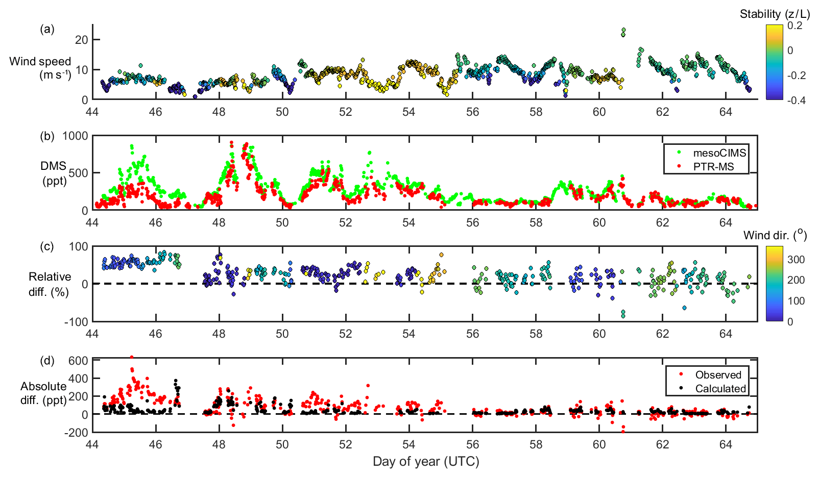
Figure 1From top to bottom, wind speed and stability (a), DMSa measurements from mesoCIMS and PTR-MS (b), relative difference (normalised to mesoCIMS) according to absolute wind direction (c), and absolute observed and calculated difference between mesoCIMS and PTR-MS (d), taking into account the expected DMS concentration gradient (Eq. 1).
Figure 1 shows wind speed, absolute wind direction and atmospheric stability, DMSa levels from the voyage measured by PTR-MS and mesoCIMS, relative percent difference between the two measurements (normalised to the mesoCIMS), and observed absolute difference in DMSa between the two measurements, as well as the expected calculated difference (Eq. 1) between the two measurements due to the DMSa concentration gradient.
The mesoCIMS and PTR-MS DMSa data showed similar temporal behaviour over the voyage (Fig. 1). From DOY 44 to 46 there was an average of 50 % (± 10 %) relative difference between measurements, yet on DOY 47 this difference decreased suddenly to an average of ∼ 20 % (± 20 %).
Overall, agreement between instruments improved with time during the voyage, with differences of several hundred parts per trillion (ppt) of DMS observed in the first few days decreasing to differences of only 10–20 ppt by the end of the voyage. The agreement between instruments improves with increasing wind speeds (Fig. 1). The expected calculated difference between DMSa at the two inlet heights due to the DMS concentration gradient also decreases throughout the voyage. This indicates that the increasing agreement between instruments during the voyage was likely influenced by a progressively well-mixed atmosphere leading to weaker DMS vertical gradients.
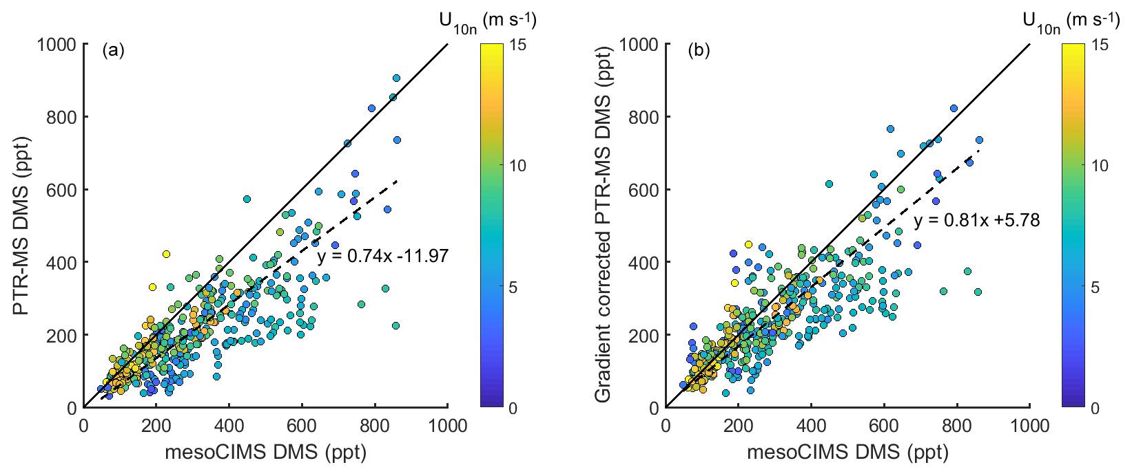
Figure 2(a) DMSa measured by mesoCIMS (x axis) and PTR-MS (y axis) (b) mesoCIMS (x axis) and PTR-MS (y axis) DMS data corrected for the expected concentration gradient (observed PTR-MS DMS + calculated delta DMS). Dashed lines represent the reduced major axis regression and solid lines represent a 1 : 1 relationship.
The reason for the improved agreement between mesoCIMS and PTR-MS at DOY 47 is unlikely due to a decrease in the DMS concentration gradient (Fig. 1d, bottom panel), but it is more likely due to changes in instrument calibration or other differences. However, careful inspection of the instrument parameters, configurations and calibration responses prior to DOY 47 did not identify the cause of the disagreement.
Figure 2a shows paired DMSa data from the mesoCIMS versus PTR-MS over the whole voyage, and Fig. 2b shows paired mesoCIMS data versus PTR-MS data converted to the same height as the mesoCIMS with the expected DMS difference calculated from the eddy covariance estimate of DMS flux (from mesoCIMS) and eddy diffusivity (PTR-MS DMSa+ calculated difference between the two intake heights). The reduced major axis regression relationship between the two measurement systems for uncorrected data gives a slope of 0.74±0.02, while for the corrected data the relationship gives 0.81±0.02 (R2=0.69). The gradient-corrected slope agrees with the ambient bag sample ratio from the method comparison (PTR-MS ∕ mesoCIMS ) (Table 1). Correcting for the DMS gradient improved the comparison between PTR-MS and mesoCIMS. The remaining ∼ 20 % difference is likely due to instrument calibration differences and differing approaches of integrated versus discrete measurements.
There was no obvious impact of absolute wind direction on the differences observed between measurement systems. Note that due to the baseline switch which was employed to avoid sampling ship exhaust down the PTR-MS inlet (Lawson et al., 2015), the PTR-MS did not sample during certain relative wind directions. However, this does not affect the comparison which was undertaken only when data were available for both instruments.
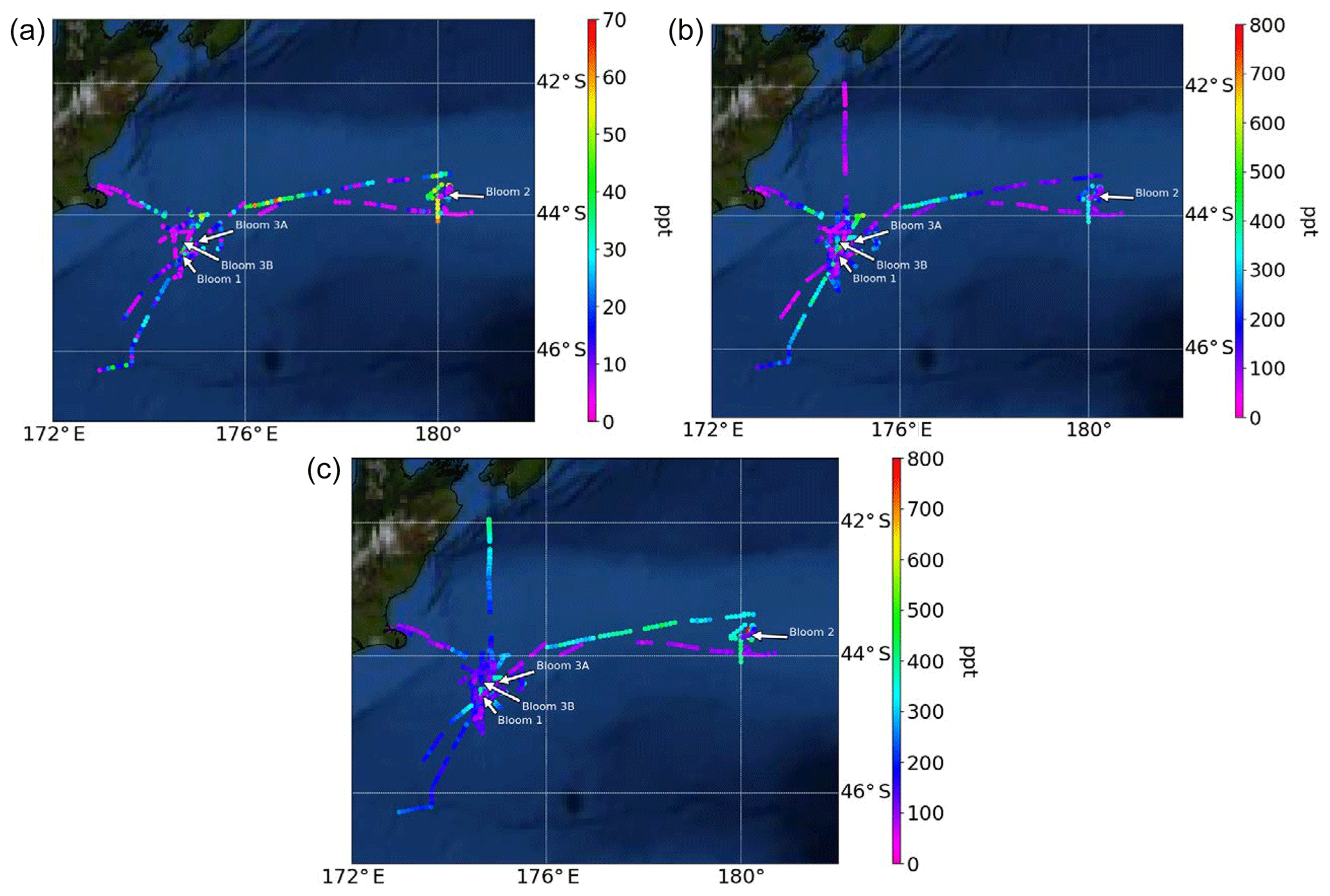
Figure 3Atmospheric mixing ratios of (a) MeSHa, (b) DMSa and (c) acetonea as a function of the voyage track. Location of the blooms are shown.
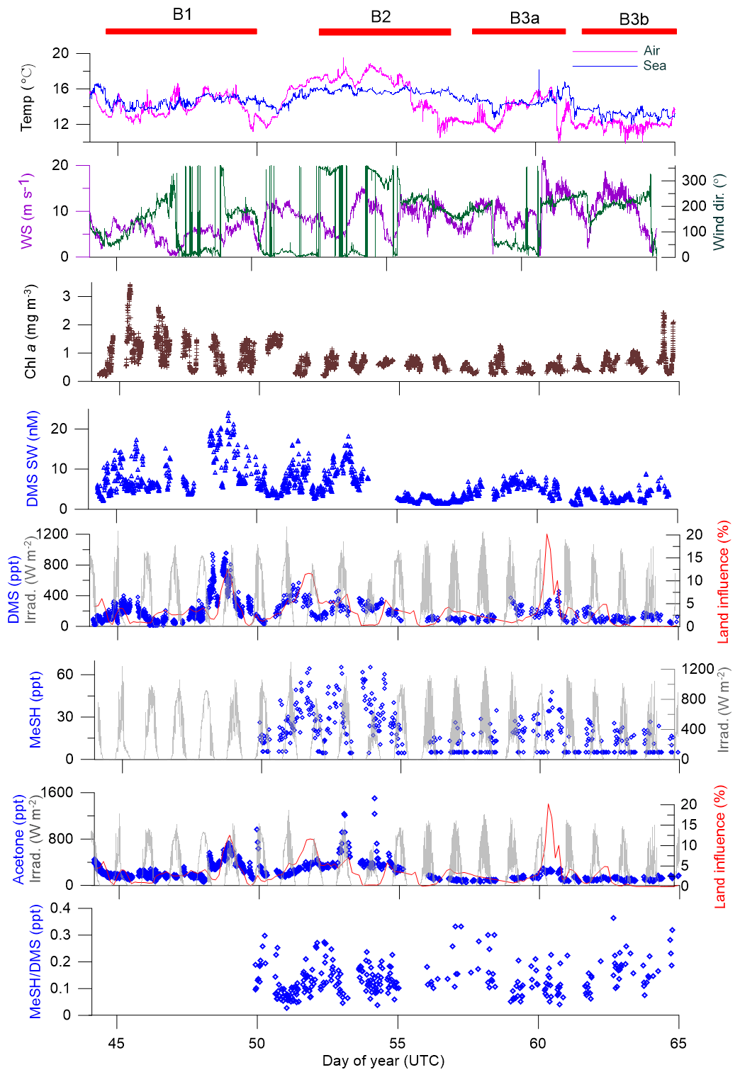
Figure 4Time series of measurements during the SOAP voyage according to DOY. Atmospheric DMS and MeSH measurements below detection limit have had half detection limit substituted. WS represents wind speed, wind dir represents wind direction, Irrad. represents irradiance and Chl a represents chlorophyll a.
3.2 Ambient atmospheric data
Atmospheric mixing ratios of MeSHa, DMSa and acetonea are shown along the voyage track in Fig. 3 with bloom locations highlighted. Figure 4 shows a time series of MeSHa, DMSa, acetonea and MeSHa ∕ DMSa (all measured with PTR-MS), as well as DMSsw (miniCIMS) from Bell et al. (2015), Chl a, irradiance, wind speed, wind direction, and sea and air temperature. Note that MeSHa measurements started on DOY 49 (the last day of bloom B1). The fraction of backward trajectories arriving at the ship that had been in contact with land masses in the previous 10 days is also shown with a value of 0 indicating no contact with land masses in the preceding 10 days. This was calculated using the Lagrangian Numerical Atmospheric-dispersion Modelling Environment (NAME) for the lower atmosphere (0–100 m) as time-integrated particle density (g s m−3), every 3 h from the ship location (Jones et al., 2007) as shown in Law et al. (2017). Where air contacted land masses, this was the New Zealand land mass in almost all cases.
Table 2MeSHa, DMSa and acetonea measured with PTR-MS during the SOAP voyage, with reaction rate constant for OH and calculated lifetime with respect to OH.
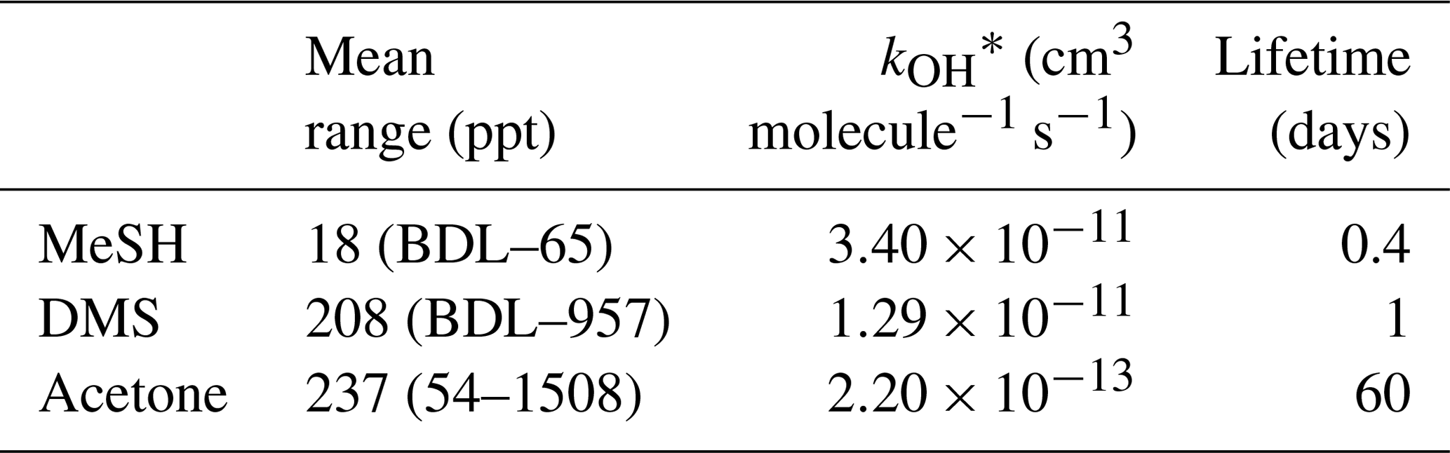
BDL represents below detection limit. * Reaction rate constants from Atkinson (1997) (MeSH), Berresheim et al. (1987) (DMS) and Atkinson (1986) (acetone).
MeSHa ranged from below detection limit (< 10 ppt) to 65 ppt, DMSa ranged from below detection limit (∼ 22 ppt) up to 957 ppt, and acetonea ranged from 50 to 1500 ppt (Table 2). The ratio of MeSHa to DMSa ranged from 0.03 to 0.36 (mean 0.14) for measurements when both were above the minimum detectable limit. Periods of elevated DMSa generally correspond to periods of elevated DMSsw. Both DMSa and DMSsw were very high during B1, during the transect to B2, and the first half of B2 occupation. MeSHa variability broadly correlates with DMSa and DMSsw, with highest levels during B2 (no data available for B1). The highest acetonea levels observed occur during B2, and a broad acetone peak during B1 of 700 ppt (∼ DOY 49) overlaps with but is slightly offset from the largest DMSa peak during the voyage (∼ 957 ppt). DMSa, acetonea and MeSHa were somewhat lower during B3a and lowest during B3b (the post-storm part of that bloom B3) (see Law et al., 2017). In general, DMSa levels during B1 were at the upper range of those found in prior studies elsewhere (Lana et al., 2011; Law et al., 2017). MeSHa levels during B2 ranged from below detection limit (∼ 10 ppt) up to 65 ppt (mean 25 ppt), which is substantially higher than the only comparable measurements from the Drake Passage and the coastal and inshore waters west of the Antarctic Peninsula (3.6 ppt) (Berresheim, 1987). The average acetonea levels during this study were broadly comparable to those from similar latitudes reported in the South Atlantic and Southern Ocean (Williams et al., 2010) and at Cape Grim (Galbally et al., 2007). Acetonea during SOAP was generally lower than at similar latitudes at Mace Head (Lewis et al., 2005), the southern Indian Ocean (Colomb et al., 2009) and also the marine subtopics (Read et al., 2012; Schlundt et al., 2017; Warneke and de Gouw, 2001; Williams et al., 2004).
There were two occasions when elevated acetonea corresponded closely to an increased land influence – during B1 on DOY 48–49 (maximum land influence 12 %) and DOY 60 (maximum land influence 20 %) (Fig. 4). Both these periods corresponded to winds from the north, and back trajectories show that the land mass contacted was the southern tip of New Zealand's North Island (including the city of Wellington and the northern section of the South Island in both cases). The acetone measured during these periods may have been emitted from anthropogenic and biogenic sources as well as from photochemical oxidation of hydrocarbon precursors (Fischer et al., 2012). The acetone enhancement relative to the degree of land influence was higher on DOY 48–49 than DOY 60 possibly due to different degrees of dilution of the terrestrial plume or different terrestrial source strengths.
The period with the highest acetone levels during B2 (1508 ppt) corresponds with a period of negligible land influence (0.3 %), indicating a non-terrestrial, possibly local, source of acetonea. Neither MeSHa nor DMSa maxima corresponded with peaks in land influence, except for the latter part of the DMSa maximum on DOY 48–49; however, the source of DMSa during DOY 48–49 is attributed to local ocean emissions as shown by strong association between DMSsw and DMSa during this period (Fig. 4).

Figure 5Correlation between (a) DMSa and MeSHa all data (DOY 49 onwards) and (b) DMSa and MeSHa bloom (B2) only.
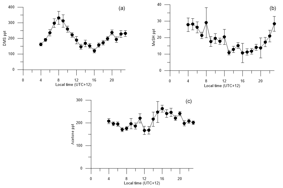
Figure 6Diurnal cycles of (a) DMSa, (b) MeSHa, (c) acetonea with land-influenced data removed. Average values from 00:00 to 03:00 are excluded because of lower data collection during this period, due to calibrations and zero air measurements.
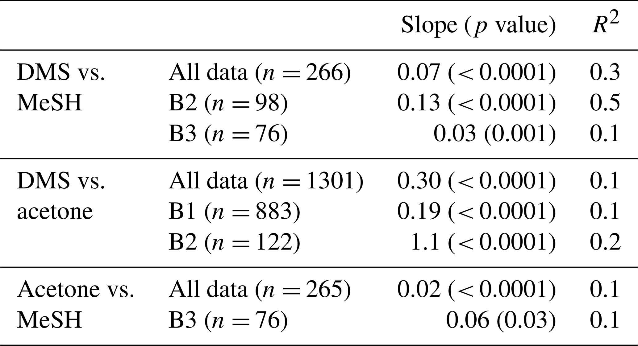
Correlations of DMSa, MeSHa and acetonea were examined to identify possible common marine sources or processes influencing atmospheric levels (Table 3). Only data above the minimum detectable limit were included in the regressions. Acetonea data likely influenced by terrestrial sources (DOY 48–49 and 60, described above) were removed from this analysis. A moderate correlation (R2=0.5, p<0.0001) was found between DMSa and MeSHa during B2 with a correlation of R2=0.3, (p<0.0001) between DMSa and MeSHa for all data (Fig. 5). During B2 the slope was 0.13 (MeSHa roughly 13 % of the DMSa mixing ratios), while for all data the slope was 0.07 (including blooms and transiting between blooms).
Table 3Pearson correlations between DMSa, MeSHa and acetonea, which are significant at the 95 % confidence interval. Land-influenced data were removed (acetone).
MeSHsw and DMSsw are produced from bacterial catabolism of DMSP via two competing processes, so the amount of DMSsw vs. MeSHsw produced from DMSP will depend on the relative importance of these two pathways at any given time. Additional sources of DMSsw, such as phytoplankton that cleave DMSP into DMS, will also influence the amount of DMSsw vs. MeSHsw produced. A phytoplankton-mediated source of DMSsw was likely to be an important contributor to the DMSsw pool during the SOAP voyage, either through indirect processes (zooplankton grazing, viral lysis and senescence) or direct processes (algal DMSP-lyase activity) (Lizotte et al., 2017). The relative loss rates of DMSsw and MeSHsw through oxidation, bacterial uptake or reaction with DOM will also influence the amount of each gas available to transfer to the atmosphere, with MeSHsw having a much faster loss rate in seawater than DMSsw (Kiene and Linn, 2000; Kiene et al., 2000). Differences between the gas transfer velocities of DMS and MeSH would also affect the atmospheric mixing ratios. Such differences are likely to be small, due to similar solubilities (Sander, 2015) and diffusivities (Johnson, 2010). A final factor that will influence the slope of DMSa vs. MeSHa is the atmospheric lifetime (Table 2). The average lifetimes of DMSa and MeSHa in this study are estimated at 24 and 9 h, respectively, with respect to OH, calculated using DMS reaction rate of OH from Berresheim et al. (1987), the MeSH reaction rate from Atkinson et al. (1997) and OH concentration calculated as described in Lawson et al. (2015). Hence, the correlation between DMSa and MeSHa reflects the common seawater source of both gases, while the differing slopes between B2 and all data probably reflect the different sources and atmospheric lifetimes. While a correlation between MeSH and DMS has been observed in seawater samples previously (Kettle et al., 2001; Kiene et al., 2017), to our knowledge this is the first time that a correlation between MeSHa and DMSa has been observed in the atmosphere over the remote ocean.
There were several weak (R2≤0.2) but significant correlations between DMSa and acetonea and acetonea and MeSHa (Table 3). The correlation of acetonea with DMSa may reflect elevated organic sources for photochemical production of acetone in regions of high dissolved sulfur species. A further discussion of drivers of DMSa, acetonea and MeSHa mixing ratios is provided in Sect. 3.3.
An additional factor which may influence the measured mixing ratios of DMSa, MeSHa and acetonea is entrainment of air from the free troposphere into the MBL. For short-lived DMS and MeSH (Table 2), free tropospheric air is most likely to be depleted in these gases compared to air sampled close to the ocean surface. Acetone is relatively long lived (Table 2) and has significant terrestrial sources (Fischer et al., 2012), and so, depending on the origin of the free tropospheric air, it could be enhanced or depleted relative to MBL air.
Figure 6 shows the voyage-average diurnal cycles for DMSa, MeSHa and acetonea. The diurnal cycle of DMSa shows variations by almost a factor of 3 from morning (maximum at 08:00, ∼ 330 ppt) to late afternoon (minimum, 16:00, ∼ 120 ppt). A DMSa diurnal cycle with sunrise maximum and late afternoon minimum has been observed in many previous studies and is attributed to photochemical destruction by OH. This includes Cape Grim baseline station, which samples air from the Southern Ocean (average minimum and maximum ∼ 40–70 ppt) (Ayers and Gillett, 2000), over the tropical Indian ocean (average minimum and maximum ∼ 25–60 ppt (Warneke and de Gouw, 2001) and at Kiritimati in the tropical Pacific (average minimum and maximum 120–200 ppt) (Bandy et al., 1996). The higher atmospheric levels in this study are due to high DMSsw concentrations (> 15 nM). The amplitude of the DMS diurnal cycle is likely to have been influenced by stationing the vessel over blooms with high DMSsw from 08:00 each day and regional mapping of areas with lower DMSsw overnight (Law et al., 2017).
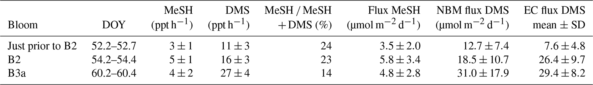
Table 4MeSH and DMS fluxes calculated using the nocturnal buildup method (NBM) compared with DMS flux measured using the eddy covariance (EC) method (Bell et al., 2015). The ± values on the MeSH and DMS fluxes are due to the standard deviation (SD) of the MBL height.
The diurnal cycle for MeSHa (Fig. 6b) shows similar behaviour to DMSa with the mixing ratios varying by a factor of ∼ 2 with the minimum mixing ratio occurring at around 16:00 (the same time as minimum DMSa). The most important sink of MeSHa is thought to be oxidation by OH (Lee and Brimblecombe, 2016), and the minima in late afternoon may be due to destruction by OH. The decoupling of the DMS and MeSH diurnal cycles between 04:00 and 08:00, with DMS increasing and MeSH decreasing, is likely due to the differing production pathways as well as the possibility of additional sinks for MeSH in the ocean during this time. This period may also have been influenced by mapping areas with lower DMSsw overnight and stationing the vessel over blooms with high DMSsw from 08:00 each day, as described above.
The acetonea diurnal cycle (Fig. 6c) with land-influenced data removed shows reasonably consistent mixing ratios from the early morning until midday, with an overall increase in acetone levels during the afternoon hours from 14:00 onwards, then decreasing again at night, which is the opposite to the behaviour of DMSa and MeSHa. Acetone is long lived (∼ 60 days – Table 2) with respect to oxidation by OH. The increase of acetonea mixing ratios in the afternoon may indicate photochemical production from atmosphere or sea surface precursors but there was no correlation between irradiance and acetonea during the voyage.
3.3 Flux calculation from nocturnal accumulation of MeSH
MeSH and DMS fluxes (F) were calculated according to the nocturnal accumulation method (Marandino et al., 2007). This approach assumes that nighttime photochemical losses are negligible and that sea surface emissions accumulate overnight within the well-mixed marine boundary layer (MBL). Horizontal homogeneity and zero flux at the top of the boundary layer are also assumed. The air–sea flux is calculated from the increase in MeSH and DMS. For example,
where [MeSH] is the concentration of MeSH (mol m−3) and h is the average nocturnal MBL for the voyage of 1135 m ± 657 m, estimated from nightly radiosonde flights.
DMS and MeSH fluxes were calculated for three nights (DOY 52, 54 and 60) (Table 4) when linear increases in mixing ratios occurred over several hours (Fig. 4). The MeSH flux was lowest on DOY 52 prior to B2 (3.5±2 µmol−1 m−2 d−1), higher on DOY 60 during B3a (4.8±2.8 µmol−1 m−2 d−1) and highest on DOY 42 during B2 (5.8±3.4 µmol−1 m−2 d−1). There are no MeSH measurements during B1. The percentage of MeSH ∕ (DMS + MeSH) emitted varied from 14 % for DOY 60 (B3a) up to 23 % and 24 % for DOY 54 (B2) and DOY 52 (prior to B2), respectively.
For comparison, the DMS fluxes measured using eddy covariance (EC) at the same time are given in Table 4 (Bell et al., 2015). DMS fluxes calculated using the nocturnal accumulation method are within the variability of the EC fluxes (Bell et al., 2015).
Table 5MeSH flux from this and previous studies (voyage averages).

The average MeSH flux calculated from this study (4.7 µmol m−2 d−1) was more than 4 times higher than average MeSH fluxes from previous studies in the North Atlantic–South Atlantic transect (Kettle et al., 2001) and in the Baltic Sea, Kattegat, and North Sea (Leck and Rodhe, 1991) (Table 5). The MeSH fluxes calculated from this work are comparable to maximum values reported by Kettle et al. (2001), which were observed in localised coastal and upwelling regions. The average emission of MeSH compared to DMS (MeSH ∕ (DMS + MeSH)) was higher in this study (20 %) compared to previous studies (Table 5) including the Baltic Sea, Kattegat, and North Sea (5 %, 4 % and 11 %); North Atlantic–South Atlantic (16 %); and a recent study from the northeast subarctic Pacific (∼ 15 %) (Kiene et al., 2017). Note that other sulfur species such as dimethyl disulfide (DMDS), carbon disulfide (CS2) and hydrogen sulfide (H2S) typically make a very small contribution to the total sulfur compared to DMS and MeSH (Leck and Rodhe, 1991; Kettle et al., 2001; Yvon et al., 1993), and so they are neglected from this calculation.
3.4 Correlation with ocean biogeochemistry
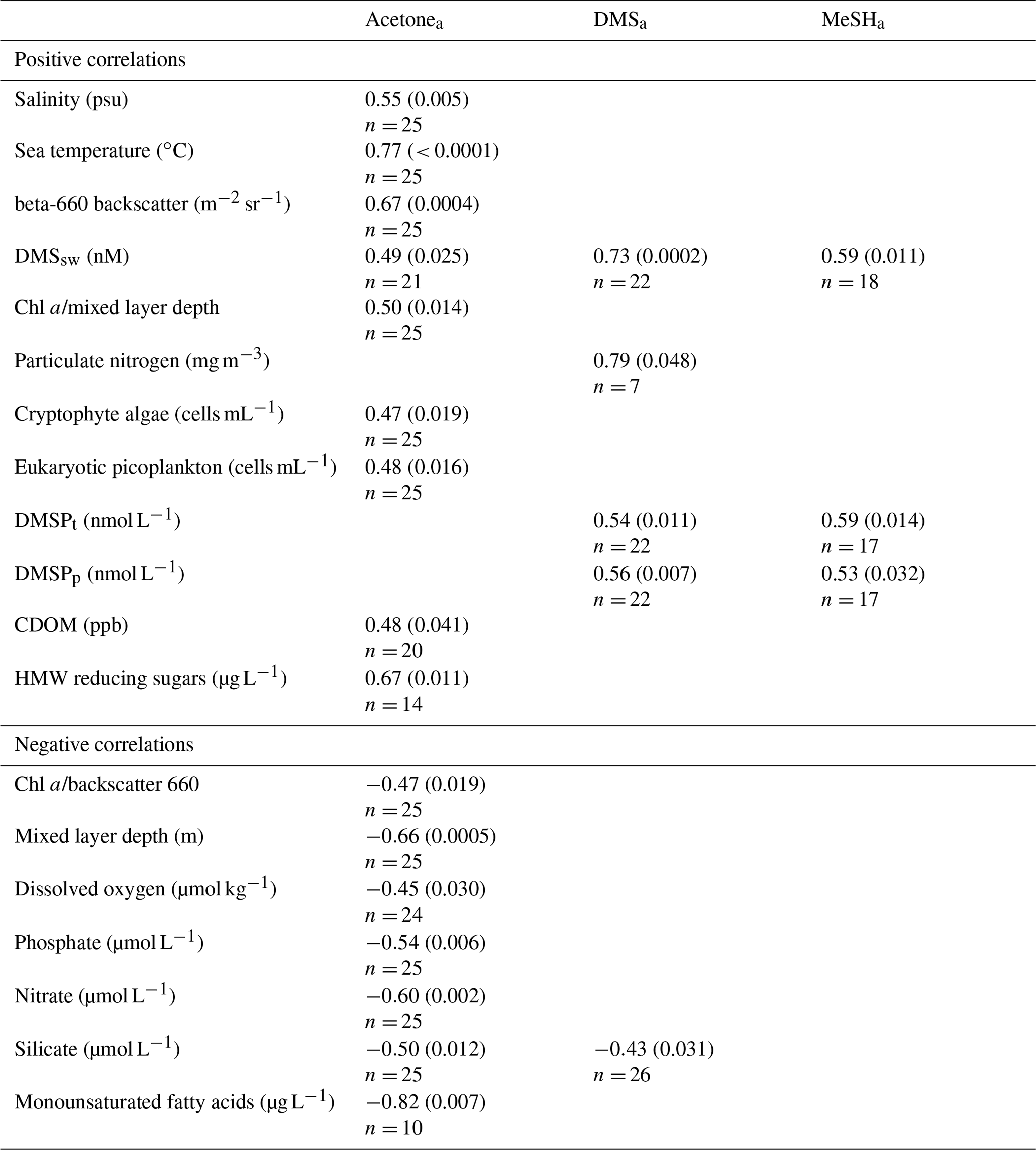
To investigate the influence of biogeochemical parameters on atmospheric mixing ratios of MeSHa, DMSa and acetonea, Spearman rank correlations were undertaken to identify relationships significant at the 95 % confidence interval (CI). Table 6 summarises the correlation coefficients and p values for significant correlations. MeSHa, DMSa and acetonea data were averaged for 1 h either side of the CTD water entry time for the analysis.
Sulfur gases MeSHa and DMSa are short lived and so the air–sea flux is controlled by the seawater concentration. By contrast, acetonea is much longer lived in the atmosphere (∼ 60 days), so the air–sea gradient can be influenced by both oceanic emissions and atmospheric transport from other sources. As such, the variability in acetonea mixing ratios may be driven by ocean–air exchange and/or input of acetonea to the boundary layer from terrestrial sources, the upper atmosphere or in situ production. This means that correlation analyses to explore ocean biogeochemical sources of acetonea may be confounded by atmospheric sources. Removal of land-influenced data reduces the likelihood of this, but observed increases in atmospheric acetone could still be from in situ processes such as oxidation of organic aerosol or mixing from above the boundary layer.
Both MeSHa and DMSa have a strong positive and highly significant relationship with DMSsw, and a moderate correlation with discrete measurements of DMSPt (total) and DMSPp (particulate). The correlation of DMSa with DMSsw can be attributed to the positive flux of DMS out of the ocean; however, the correlation of MeSHa with DMSsw is likely due to a common ocean precursor of both gases (DMSP), albeit via different production pathways. DMSa and MeSHa correlate with DMSPp (particulate) but not with DMSPd (dissolved). For DMSa, the correlation may reflect that a proportion of the DMS observed was derived directly from phytoplankton rather than being bacterially mediated, which is in agreement with findings by Lizotte et al. (2017); however, as demethylation of DMSPd represents the primary source of MeSH, the lack of correlation is surprising. The latter may reflect MeSH sinks in surface water associated with organics and particles (Kiene, 1996), and this could be confirmed via incubation experiments. DMSa also correlated with particulate nitrogen and showed a moderate negative correlation with silicate that may reflect lower DMS production in diatom-dominated waters.
Acetonea shows a positive correlation with temperature and negative correlation with nutrients. This is consistent with reported sources of acetonesw in warmer subtropical waters (Beale et al., 2013; Yang et al., 2014a; Tanimoto et al., 2014; Schlundt et al., 2017). The positive relationship with organic material including HMW sugars and CDOM may reflect a photochemical ocean source (Zhou and Mopper, 1997; Dixon et al., 2013; de Bruyn et al., 2012; Kieber et al., 1990) or possibly a biological source (Nemecek-Marshall et al., 1995, 1999; Schlundt et al., 2017; Sinha et al., 2007; Halsey et al., 2017) as indicated by the correlations with cryptophyte and picoeukaryote abundance. Correlation with particle backscatter suggests potential links between acetonea and coccolithophores (Sinha et al., 2007). Alternatively, the positive correlations of acetonea with these organic components of sea water may reflect acetone production in the atmosphere from photochemical oxidation of ocean-derived organic aerosols (Pan et al., 2009; Kwan et al., 2006; Jacob et al., 2002). Seawater acetone measurements would allow for further elucidation of the relationships between acetonea and biogeochemical parameters identified in this study. More generally, mesocosm or laboratory studies could be employed to identify the explicit sources and production mechanisms of these gases in Chatham Rise waters.
Table 6Spearman rank correlations between acetonea, DMSa and MeSHa, as well as biogeochemical parameters, using data from the 14 February–4 March 2012 (acetonea, DMSa) and 20 February–4 March 2012 (MeSHa). Correlations shown are significant at the 95 % confidence interval (CI). Correlation coefficient (and p value) are shown. No entry indicates there was no correlation at 95 % CI. Land-influenced acetonea data excluded (see text for details).
Mixing ratios of short-lived MeSHa over the remote ocean of up to 65 ppt in this study are the highest observed to date, and they provide evidence that MeSH transfers from the ocean into the atmosphere and may be present at non-negligible levels in the atmosphere over other regions of high biological productivity. The average MeSH flux calculated from this study (4.7 µmol m−2 d−1) was at least 4 times higher than average MeSH fluxes from previous studies, and it is comparable to maximum MeSH flux values reported in localised coastal and upwelling regions of the North Atlantic–South Atlantic (Kettle et al., 2001) (Table 5). The average emission of MeSH compared to DMS (MeSH ∕ (DMS + MeSH)) was higher in this study (20 %) compared to previous studies (4 %–16 %), indicating that MeSH provides a significant transfer of sulfur to the atmosphere in this region. Taken together with other studies, the magnitude of the ocean MeSH flux to the atmosphere appears to be highly variable as is the proportion of S emitted as MeSH compared to DMS. For example, MeSH fluxes in the Kettle et al. (2001) study varied by several orders of magnitude, and in some cases the MeSH flux equalled the DMS flux. Similarly, DMSsw ∕ MeSHsw concentration ratios have varied substantially (Kettle et al., 2001, Leck and Rodhe, 1991; Kiene et al., 2017). As such, further studies are needed to investigate the spatial distribution of MeSH both in seawater and the atmosphere as well as the importance of MeSH as a source of atmospheric sulfur. The fate of atmospheric MeSH sulfur in the atmosphere is also highly uncertain, in terms of its degradation pathways, reactions, and intermediate and final degradation products. For example, the impact that oxidation of MeSHa has on the oxidative capacity of the MBL, and on other processes such as particle formation or growth, to the best of our knowledge remains largely unknown, and further work is needed on its atmospheric processes and fate.
A correlation analysis of MeSHa and biogeochemical parameters was undertaken for the first time, and it showed that MeSHa, as well as DMSa, correlated with their ocean precursor, DMSP, and also correlated with seawater DMS (DMSsw). The correlation of MeSHa with DMSsw is likely due to a common ocean precursor of both gases (DMSP), which is produced via different pathways.
Correlation of acetonea with biogeochemical parameters suggests a source of acetone from warmer subtropical ocean waters, in line with other studies, with positive correlations between acetonea and ocean temperature, high-molecular-weight sugars, cryptophyte, eukaryote phytoplankton, chromophoric dissolved organic matter (CDOM), and particle backscatter, and a negative correlation with nutrients. While data with a terrestrial source influence were removed from this analysis, it is still possible that the acetone peaks observed may not have been due to a positive flux of acetone from the ocean but rather from in situ processes, leading to acetone production such as oxidation of marine-derived organic aerosol.
Finally, the SOAP voyage provided the opportunity to compare three independently calibrated DMSa measurement techniques at sea (PTR-MS, mesoCIMS and GC-SCD). Agreement between the three techniques was generally good; however, some systematic differences between the datasets were observed. Some of these differences were attributed to the near-surface DMS gradient and the use of different inlet heights (28 and 12 m a.s.l. for the PTR-MS and mesoCIMS, respectively), as well as differing approaches of integrated versus discrete measurements. The remaining discrepancies are likely due to differences in calibration scales, suggesting that further investigation of the stability and/or absolute calibration of DMS standards used at sea is warranted.
DMS, acetone and MeSH data are available via the CSIRO data access portal (DAP) at https://doi.org/10.25919/5d914b00c5759 (Lawson, 2019). Further data are available by emailing the corresponding author or the voyage leader: cliff.law@niwa.co.nz.
The supplement related to this article is available online at: https://doi.org/10.5194/acp-20-3061-2020-supplement.
SJL wrote the paper. CSL led the research voyage. All authors operated instrumentation during the voyage and contributed data. All authors contributed to data analysis and/or interpretation.
The authors declare that they have no conflict of interest.
This article is part of the special issue “Surface Ocean Aerosol Production (SOAP) (ACP/OS inter-journal SI)”. It is not associated with a conference.
We thank the officers and crew of the RV Tangaroa and NIWA vessels for logistics support. Many thanks to John McGregor (NIWA) for providing land influence data and to Paul Selleck and Erin Dunne (CSIRO) for helpful discussions. Thanks to the NIWA Visiting Scientist Scheme and CSIRO's Capability Development Fund for providing financial support for Sarah Lawson's participation in the SOAP voyage.
This paper was edited by Mario Hoppema and reviewed by Cathleen Schlundt and one anonymous referee.
Alcolombri, U., Ben-Dor, S., Feldmesser, E., Levin, Y., Tawfik, D. S., and Vardi, A.: Identification of the algal dimethyl sulfide–releasing enzyme: A missing link in the marine sulfur cycle, Science, 348, 1466–1469, https://doi.org/10.1126/science.aab1586, 2015.
Atkinson, R.: Kinetics and mechanisms of the gas-phase reactions of the hydroxyl radical with organic compounds under atmospheric conditions, Chem. Rev., 86, 69–201, https://doi.org/10.1021/cr00071a004, 1986.
Atkinson, R., Baulch, D. L., Cox, R. A., Hampson, R. F., Kerr, J. A., Rossi, M. J., and Troe, J.: Evaluated Kinetic, Photochemical and Heterogeneous Data for Atmospheric Chemistry: Supplement V. – IUPAC Subcommittee on Gas Kinetic Data Evaluation for Atmospheric Chemistry, J. Phys. Chem. Ref. Data, 26, 521–1011, https://doi.org/10.1063/1.556011, 1997.
Ayers, G. P. and Gillett, R. W.: DMS and its oxidation products in the remote marine atmosphere: implications for climate and atmospheric chemistry, J. Sea Res., 43, 275–286, 2000.
Bandy, A. R., Thornton, D. C., Blomquist, B. W., Chen, S., Wade, T. P., Ianni, J. C., Mitchell, G. M., and Nadler, W.: Chemistry of dimethyl sulfide in the equatorial Pacific atmosphere, Geophys. Res. Lett., 23, 741–744, https://doi.org/10.1029/96gl00779, 1996.
Beale, R., Dixon, J. L., Arnold, S. R., Liss, P. S., and Nightingale, P. D.: Methanol, acetaldehyde, and acetone in the surface waters of the Atlantic Ocean, J. Geophys. Res.-Oceans, 118, 5412–5425, https://doi.org/10.1002/jgrc.20322, 2013.
Beale, R., Dixon, J. L., Smyth, T. J., and Nightingale, P. D.: Annual study of oxygenated volatile organic compounds in UK shelf waters, Mar. Chem., 171, 96–106, https://doi.org/10.1016/j.marchem.2015.02.013, 2015.
Bell, T. G., De Bruyn, W., Miller, S. D., Ward, B., Christensen, K. H., and Saltzman, E. S.: Air–sea dimethylsulfide (DMS) gas transfer in the North Atlantic: evidence for limited interfacial gas exchange at high wind speed, Atmos. Chem. Phys., 13, 11073–11087, https://doi.org/10.5194/acp-13-11073-2013, 2013.
Bell, T. G., De Bruyn, W., Marandino, C. A., Miller, S. D., Law, C. S., Smith, M. J., and Saltzman, E. S.: Dimethylsulfide gas transfer coefficients from algal blooms in the Southern Ocean, Atmos. Chem. Phys., 15, 1783–1794, https://doi.org/10.5194/acp-15-1783-2015, 2015.
Berresheim, H.: Biogenic sulfur emissions from the Subantarctic and Antarctic Oceans, J. Geophys. Res., 92, 13245–13262, https://doi.org/10.1029/JD092iD11p13245, 1987.
Burrell, T. J.: Bacterial extracellular enzyme activity in a future ocean, PhD thesis, Victoria University of Wellington, 324 pp., 2015.
Carpenter, L. J., Archer, S. D., and Beale, R.: Ocean-atmosphere trace gas exchange, Chem. Soc. Rev., 41, 6473–6506, https://doi.org/10.1039/c2cs35121h, 2012.
Carpenter, L. J. and Nightingale, P. D.: Chemistry and Release of Gases from the Surface Ocean, Chem. Rev., 115, 4015–4034, https://doi.org/10.1021/cr5007123, 2015.
Charlson, R., Lovelock, J., Andreae, M., and Warren, S.: Oceanic phytoplankton, atmospheric sulphur, cloud albedo and climate, Nature, 326, 655–661, https://doi.org/10.1038/326655a0, 1987.
Colomb, A., Gros, V., Alvain, S., Sarda-Esteve, R., Bonsang, B., Moulin, C., Klupfel, T., and Williams, J.: Variation of atmospheric volatile organic compounds over the Southern Indian Ocean (30-49∘ S), Environ. Chem., 6, 70–82, https://doi.org/10.1071/en08072, 2009.
de Bruyn, W. J., Clark, C. D., Pagel, L., and Takehara, C.: Photochemical production of formaldehyde, acetaldehyde and acetone from chromophoric dissolved organic matter in coastal waters, J. Photoch. Photobio. A, 226, 16–22, https://doi.org/10.1016/j.jphotochem.2011.10.002, 2012.
Dixon, J. L., Beale, R., and Nightingale, P. D.: Production of methanol, acetaldehyde, and acetone in the Atlantic Ocean, Geophys. Res. Lett., 40, 4700–4705, https://doi.org/10.1002/grl.50922, 2013.
Feilberg, A., Liu, D., Adamsen, A. P. S., Hansen, M. J., and Jonassen, K. E. N.: Odorant Emissions from Intensive Pig Production Measured by Online Proton-Transfer-Reaction Mass Spectrometry, Environ. Sci. Technol., 44, 5894–5900, https://doi.org/10.1021/es100483s, 2010.
Fischer, E. V., Jacob, D. J., Millet, D. B., Yantosca, R. M., and Mao, J.: The role of the ocean in the global atmospheric budget of acetone, Geophys. Res. Lett., 39, L01807, https://doi.org/10.1029/2011gl050086, 2012.
Flöck, O. R. and Andreae, M. O.: Photochemical and non-photochemical formation and destruction of carbonyl sulfide and methyl mercaptan in ocean waters, Mar. Chem., 54, 11–26, https://doi.org/10.1016/0304-4203(96)00027-8, 1996.
Galbally, I. E., Lawson, S. J., Weeks, I. A., Bentley, S. T., Gillett, R. W., Meyer, M., and Goldstein, A. H.: Volatile organic compounds in marine air at Cape Grim, Australia, Environ. Chem., 4, 178–182, https://doi.org/10.1071/en07024, 2007.
Gall, M. P., Davies-Colley, R. J., and Merrilees, R. A.: Exceptional visual clarity and optical purity in a sub-alpine lake, Limnol. Oceanogr., 58, 443–451, https://doi.org/10.4319/lo.2013.58.2.0443, 2013.
Hall, J. A. and Safi, K.: The impact of in situ Fe fertilisation on the microbial food web in the Southern Ocean, Deep-Sea Res. Pt II, 48, 2591–2613, https://doi.org/10.1016/S0967-0645(01)00010-8, 2001.
Halsey, K. H., Giovannoni, S. J., Graus, M., Zhao, Y., Landry, Z., Thrash, J. C., Vergin, K. L., and de Gouw, J.: Biological cycling of volatile organic carbon by phytoplankton and bacterioplankton, Limnol. Oceanogr., 62, 2650–2661, https://doi.org/10.1002/lno.10596, 2017.
ISO: ISO 6879: Air Quality, Performance Characteristics and Related Concepts for Air Quality Measuring Methods, International Organisation for Standardisation, Geneva, Switzerland, 1995.
Jacob, D. J., Field, B. D., Jin, E. M., Bey, I., Li, Q. B., Logan, J. A., Yantosca, R. M., and Singh, H. B.: Atmospheric budget of acetone, J. Geophys. Res.-Atmos., 107, 4100, https://doi.org/10.1029/2001jd000694, 2002.
Johnson, M. T.: A numerical scheme to calculate temperature and salinity dependent air-water transfer velocities for any gas, Ocean Sci., 6, 913–932, https://doi.org/10.5194/os-6-913-2010, 2010.
Jones, A. R., Thomson, D. J., Hort, M., and Devenish, B.: The UK Met Office's next-generation atmospheric dispersion model, NAME III, in: Proceedings of the 27th NATO/CCMS International Technical Meeting on Air Pollution Modelling and its Application, edited by: Borrego, C. and Norman, A.-L., Springer, 580–589, 2007.
Kettle, A. J., Rhee, T. S., von Hobe, M., Poulton, A., Aiken, J., and Andreae, M. O.: Assessing the flux of different volatile sulfur gases from the ocean to the atmosphere, J. Geophys. Res., 106, 12193–12209, https://doi.org/10.1029/2000jd900630, 2001.
Kieber, R. J., Zhou, X., and Mopper, K.: Formation of carbonyl compounds from UV-induced photodegradation of humic substances in natural waters: Fate of riverine carbon in the sea, Limnol. Oceanogr., 35, 1503–1515, https://doi.org/10.4319/lo.1990.35.7.1503, 1990.
Kiene, R. P.: Production of methanethiol from dimethylsulfoniopropionate in marine surface waters, Mar. Chem., 54, 69–83, https://doi.org/10.1016/0304-4203(96)00006-0, 1996.
Kiene, R. P. and Linn, L. J.: The fate of dissolved dimethylsulfoniopropionate (DMSP) in seawater: tracer studies using 35S-DMSP, Geochim. Cosmochim. Ac., 64, 2797–2810, https://doi.org/10.1016/S0016-7037(00)00399-9, 2000.
Kiene, R. P., Linn, L. J., and Bruton, J. A.: New and important roles for DMSP in marine microbial communities, J. Sea Res., 43, 209–224, https://doi.org/10.1016/S1385-1101(00)00023-X, 2000.
Kiene, R. P., Williams, T. E., Esson, K., Tortell, P. D., and Dacey, J. W. H.: Methanethiol Concentrations and Sea-Air Fluxes in the Subarctic NE Pacific Ocean, American Geophysical Union, Fall meeting, 2017.
Kwan, A. J., Crounse, J. D., Clarke, A. D., Shinozuka, Y., Anderson, B. E., Crawford, J. H., Avery, M. A., McNaughton, C. S., Brune, W. H., Singh, H. B., and Wennberg, P. O.: On the flux of oxygenated volatile organic compounds from organic aerosol oxidation, Geophys. Res. Lett., 33, L15815, https://doi.org/10.1029/2006gl026144, 2006.
Lana, A., Bell, T. G., Simó, R., Vallina, S. M., Ballabrera-Poy, J., Kettle, A. J., Dachs, J., Bopp, L., Saltzman, E. S., Stefels, J., Johnson, J. E., and Liss, P. S.: An updated climatology of surface dimethlysulfide concentrations and emission fluxes in the global ocean, Global Biogeochem. Cy., 25, GB1004, https://doi.org/10.1029/2010gb003850, 2011.
Law, C. S., Brévière, E., de Leeuw, G., Garçon, V., Guieu, C., Kieber, D. J., Kontradowitz, S., Paulmier, A., Quinn, P. K., Saltzman, E. S., Stefels, J., and von Glasow, R.: Evolving research directions in Surface Ocean–Lower Atmosphere (SOLAS) science, Environ. Chem., 10, 1–16, https://doi.org/10.1071/EN12159, 2013.
Law, C. S., Smith, M. J., Harvey, M. J., Bell, T. G., Cravigan, L. T., Elliott, F. C., Lawson, S. J., Lizotte, M., Marriner, A., McGregor, J., Ristovski, Z., Safi, K. A., Saltzman, E. S., Vaattovaara, P., and Walker, C. F.: Overview and preliminary results of the Surface Ocean Aerosol Production (SOAP) campaign, Atmos. Chem. Phys., 17, 13645–13667, https://doi.org/10.5194/acp-17-13645-2017, 2017.
Law, C. S., Woodward, E. M. S., Ellwood, M. J., Marriner, A., Bury, S. J., and Safi, K. A.: Response of surface nutrient inventories and nitrogen fixation to a tropical cyclone in the southwest Pacific, Limnol. Oceanogr., 56, 1372–1385, https://doi.org/10.4319/lo.2011.56.4.1372, 2011.
Lawson, S.: DMS, acetone, methanethiol atmospheric data from SOAP voyage. v1. CSIRO, Data Collection, https://doi.org/10.25919/5d914b00c5759, 2019.
Lawson, S. J., Selleck, P. W., Galbally, I. E., Keywood, M. D., Harvey, M. J., Lerot, C., Helmig, D., and Ristovski, Z.: Seasonal in situ observations of glyoxal and methylglyoxal over the temperate oceans of the Southern Hemisphere, Atmos. Chem. Phys., 15, 223–240, https://doi.org/10.5194/acp-15-223-2015, 2015.
Leck, C. and Rodhe, H..: Emissions of marine biogenic sulfur to the atmosphere of northern Europe, J. Atmos. Chem., 12, 63–86, https://doi.org/10.1007/bf00053934, 1991.
Lee, C. L. and Brimblecombe, P.: Anthropogenic contributions to global carbonyl sulfide, carbon disulfide and organosulfides fluxes, Earth-Sci. Rev., 160, 1–18, https://doi.org/10.1016/j.earscirev.2016.06.005, 2016.
Lewis, A. C., Hopkins, J. R., Carpenter, L. J., Stanton, J., Read, K. A., and Pilling, M. J.: Sources and sinks of acetone, methanol, and acetaldehyde in North Atlantic marine air, Atmos. Chem. Phys., 5, 1963–1974, https://doi.org/10.5194/acp-5-1963-2005, 2005.
Liss, P. S. and Johnson, M. T. (Eds.): Ocean-Atmosphere Interactions of Gases and Particles, Springer Earth System Sciences, 315 pp., 2014.
Lizotte, M., Levasseur, M., Law, C. S., Walker, C. F., Safi, K. A., Marriner, A., and Kiene, R. P.: Dimethylsulfoniopropionate (DMSP) and dimethyl sulfide (DMS) cycling across contrasting biological hotspots of the New Zealand subtropical front, Ocean Sci., 13, 961–982, https://doi.org/10.5194/os-13-961-2017, 2017.
Malin, G.: Sulphur, climate and the microbial maze, Nature, 387, 857–858, https://doi.org/10.1038/43075, 1997.
Marandino, C. A., De Bruyn, W. J., Miller, S. D., Prather, M. J., and Saltzman, E. S.: Oceanic uptake and the global atmospheric acetone budget, Geophys. Res. Lett., 32, L15806, https://doi.org/10.1029/2005gl023285, 2005.
Marandino, C. A., De Bruyn, W. J., Miller, S. D., and Saltzman, E. S.: Eddy correlation measurements of the air/sea flux of dimethylsulfide over the North Pacific Ocean, J. Geophys. Res.-Atmos., 112, D03301, https://doi.org/10.1029/2006jd007293, 2007.
Nemecek-Marshall, M., Wojciechowski, C., Kuzma, J., Silver, G. M., and Fall, R.: Marine Vibrio species produce the volatile organic compound acetone, Appl. Environ. Microbiol., 61, 44–47, 1995.
Nemecek-Marshall, M., Wojciechowski, C., Wagner, W. P., and Fall, R.: Acetone formation in the Vibrio family: a new pathway for bacterial leucine catabolism, J. Bacteriol., 181, 7493–7499, 1999.
Nodder, S. D., Chiswell, S. M., and Northcote, L. C.: Annual cycles of deep-ocean biogeochemical export fluxes in subtropical and subantarctic waters, southwest Pacific Ocean, J. Geophys. Res.-Oceans, 121, 2405–2424, https://doi.org/10.1002/2015jc011243, 2016.
Pan, X., Underwood, J. S., Xing, J.-H., Mang, S. A., and Nizkorodov, S. A.: Photodegradation of secondary organic aerosol generated from limonene oxidation by ozone studied with chemical ionization mass spectrometry, Atmos. Chem. Phys., 9, 3851–3865, https://doi.org/10.5194/acp-9-3851-2009, 2009.
Quinn, P. K. and Bates, T. S.: The case against climate regulation via oceanic phytoplankton sulphur emissions, Nature, 480, 51–56, https://doi.org/10.1038/nature10580, 2011.
Read, K. A., Carpenter, L. J., Arnold, S. R., Beale, R., Nightingale, P. D., Hopkins, J. R., Lewis, A. C., Lee, J. D., Mendes, L., and Pickering, S. J.: Multiannual Observations of Acetone, Methanol, and Acetaldehyde in Remote Tropical Atlantic Air: Implications for Atmospheric OVOC Budgets and Oxidative Capacity, Environ. Sci. Technol., 46, 11028–11039, https://doi.org/10.1021/es302082p, 2012.
Safi, K. A., Griffiths, F. B., and Hall, J. A.: Microzooplankton composition, biomass and grazing rates along the WOCE SR3 line between Tasmania and Antarctica, Deep-Sea Res. Pt I, 54, 1025–1041, https://doi.org/10.1016/j.dsr.2007.05.003, 2007.
Sander, R.: Compilation of Henry's law constants (version 4.0) for water as solvent, Atmos. Chem. Phys., 15, 4399–4981, https://doi.org/10.5194/acp-15-4399-2015, 2015.
Schlundt, C., Tegtmeier, S., Lennartz, S. T., Bracher, A., Cheah, W., Krüger, K., Quack, B., and Marandino, C. A.: Oxygenated volatile organic carbon in the western Pacific convective center: ocean cycling, air–sea gas exchange and atmospheric transport, Atmos. Chem. Phys., 17, 10837–10854, https://doi.org/10.5194/acp-17-10837-2017, 2017.
Simó, R. and Pedrós-Alió, C.: Short-term variability in the open ocean cycle of dimethylsulfide, Glocal Biogeochem. Cy., 13, 1173–1181, https://doi.org/10.1029/1999gb900081, 1999.
Sinha, V., Williams, J., Meyerhöfer, M., Riebesell, U., Paulino, A. I., and Larsen, A.: Air-sea fluxes of methanol, acetone, acetaldehyde, isoprene and DMS from a Norwegian fjord following a phytoplankton bloom in a mesocosm experiment, Atmos. Chem. Phys., 7, 739–755, https://doi.org/10.5194/acp-7-739-2007, 2007.
Smith, M. J., Walker, C. F., Bell, T. G., Harvey, M. J., Saltzman, E. S., and Law, C. S.: Gradient flux measurements of sea–air DMS transfer during the Surface Ocean Aerosol Production (SOAP) experiment, Atmos. Chem. Phys., 18, 5861–5877, https://doi.org/10.5194/acp-18-5861-2018, 2018.
Somogyi, M.: Notes on Sugar Determination, J. Biol. Chem., 70, 599–612, 1926.
Somogyi, M.: Notes on Sugar Determination, J. Biol. Chem., 195, 19–23, 1952.
Sun, J., Todd, J. D., Thrash, J. C., Qian, Y., Qian, M. C., Temperton, B., Guo, J., Fowler, E. K., Aldrich, J. T., Nicora, C. D., Lipton, M. S., Smith, R. D., De Leenheer, P., Payne, S. H., Johnston, A. W. B., Davie-Martin, C. L., Halsey, K. H., and Giovannoni, S. J.: The abundant marine bacterium Pelagibacter simultaneously catabolizes dimethylsulfoniopropionate to the gases dimethyl sulfide and methanethiol, Nat. Microbiol., 1, 16065, https://doi.org/10.1038/nmicrobiol.2016.65, 2016.
Taddei, S., Toscano, P., Gioli, B., Matese, A., Miglietta, F., Vaccari, F. P., Zaldei, A., Custer, T., and Williams, J.: Carbon Dioxide and Acetone Air−Sea Fluxes over the Southern Atlantic, Environ. Sci. Technol., 43, 5218-5222, https://doi.org/10.1021/es8032617, 2009.
Tanimoto, H., Kameyama, S., Iwata, T., Inomata, S., and Omori, Y.: Measurement of Air-Sea Exchange of Dimethyl Sulfide and Acetone by PTR-MS Coupled with Gradient Flux Technique, Environ. Sci. Technol., 48, 526–533, https://doi.org/10.1021/es4032562, 2014.
Tyndall, G. S. and Ravishankara, A. R.: Atmospheric oxidation of reduced sulfur species, Int. J. Chem. Kinet., 23, 483–527, https://doi.org/10.1002/kin.550230604, 1991.
Walker, C. F., Harvey, M. J., Smith, M. J., Bell, T. G., Saltzman, E. S., Marriner, A. S., McGregor, J. A., and Law, C. S.: Assessing the potential for dimethylsulfide enrichment at the sea surface and its influence on air–sea flux, Ocean Sci., 12, 1033–1048, https://doi.org/10.5194/os-12-1033-2016, 2016.
Warneke, C. and de Gouw, J. A.: Organic trace gas composition of the marine boundary layer over the northwest Indian Ocean in April 2000, Atmos. Environ., 35, 5923–5933, 2001.
Williams, T. L., Adams, N. G., and Babcock, L. M.: Selected ion flow tube studies of H3O+(H2O)0.1 reactions with sulfides and thiols, Int. J. Mass Spectrom., 172, 149–159, https://doi.org/10.1016/S0168-1176(97)00081-5, 1998.
Williams, J., Holzinger, R., Gros, V., Xu, X., Atlas, E., and Wallace, D. W. R.: Measurements of organic species in air and seawater from the tropical Atlantic, Geophys. Res. Lett., 31, L23S06, https://doi.org/10.1029/2004gl020012, 2004.
Williams, J., Custer, T., Riede, H., Sander, R., Jöckel, P., Hoor, P., Pozzer, A., Wong-Zehnpfennig, S., Hosaynali Beygi, Z., Fischer, H., Gros, V., Colomb, A., Bonsang, B., Yassaa, N., Peeken, I., Atlas, E. L., Waluda, C. M., van Aardenne, J. A., and Lelieveld, J.: Assessing the effect of marine isoprene and ship emissions on ozone, using modelling and measurements from the South Atlantic Ocean, Environ. Chem., 7, 171–182, https://doi.org/10.1071/EN09154, 2010.
Yang, M., Beale, R., Liss, P., Johnson, M., Blomquist, B., and Nightingale, P.: Air–sea fluxes of oxygenated volatile organic compounds across the Atlantic Ocean, Atmos. Chem. Phys., 14, 7499–7517, https://doi.org/10.5194/acp-14-7499-2014, 2014a.
Yang, M., Blomquist, B. W., and Nightingale, P. D.: Air-sea exchange of methanol and acetone during HiWinGS: Estimation of air phase, water phase gas transfer velocities, J. Geophys. Res.-Oceans, 119, 7308–7323, https://doi.org/10.1002/2014jc010227, 2014b.
Yoch, D. C.: Dimethylsulfoniopropionate: Its Sources, Role in the Marine Food Web, and Biological Degradation to Dimethylsulfide, Appl. Environ. Microbiol., 68, 5804–5815, https://doi.org/10.1128/AEM.68.12.5804-5815.2002, 2002.
Yvon, S. A., Cooper, D. J., Koropalov, V., and Saltzman, E. S.: Atmospheric hydrogen sulfide over the equatorial Pacific (SAGA 3), J. Geophys. Res.-Atmos., 98, 16979–16983, https://doi.org/10.1029/92jd00451, 1993.
Zhou, X. and Mopper, K.: Photochemical production of low-molecular-weight carbonyl compounds in seawater and surface microlayer and their air-sea exchange, Mar. Chem., 56, 201–213, https://doi.org/10.1016/S0304-4203(96)00076-X, 1997.