the Creative Commons Attribution 4.0 License.
the Creative Commons Attribution 4.0 License.
 | 02 Mar 2020
A robust clustering algorithm for analysis of composition-dependent organic aerosol thermal desorption measurements
Emma L. D'Ambro
Siegfried Schobesberger
Cassandra J. Gaston
Felipe D. Lopez-Hilfiker
Jiumeng Liu
John E. Shilling
Joel A. Thornton
Christopher D. Cappa
One of the challenges of understanding atmospheric organic aerosol (OA) particles stems from its complex composition. Mass spectrometry is commonly used to characterize the compositional variability of OA. Clustering of a mass spectral dataset helps identify components that exhibit similar behavior or have similar properties, facilitating understanding of sources and processes that govern compositional variability. Here, we developed an algorithm for clustering mass spectra, the noise-sorted scanning clustering (NSSC), appropriate for application to thermal desorption measurements of collected OA particles from the Filter Inlet for Gases and AEROsols coupled to a chemical ionization mass spectrometer (FIGAERO-CIMS). NSSC, which extends the common density-based special clustering of applications with noise (DBSCAN) algorithm, provides a robust, reproducible analysis of the FIGAERO temperature-dependent mass spectral data. The NSSC allows for the determination of thermal profiles for compositionally distinct clusters of mass spectra, increasing the accessibility and enhancing the interpretation of FIGAERO data. Applications of NSSC to several laboratory biogenic secondary organic aerosol (BSOA) systems demonstrate the ability of NSSC to distinguish different types of thermal behaviors for the components comprising the particles along with the relative mass contributions and chemical properties (e.g., average molecular formula) of each mass spectral cluster. For each of the systems examined, more than 80 % of the total mass is clustered into 9–13 mass spectral clusters. Comparison of the average thermograms of the mass spectral clusters between systems indicates some commonality in terms of the thermal properties of different BSOA, although with some system-specific behavior. Application of NSSC to sets of experiments in which one experimental parameter, such as the concentration of NO, is varied demonstrates the potential for mass spectral clustering to elucidate the chemical factors that drive changes in the thermal properties of OA particles. Further quantitative interpretation of the thermograms of the mass spectral clusters will allow for a more comprehensive understanding of the thermochemical properties of OA particles.
- Article
(7156 KB) - Full-text XML
-
Supplement
(1789 KB) - BibTeX
- EndNote


Atmospheric particles are composed of hundreds to thousands of individual compounds (e.g., Hamilton et al., 2004; Goldstein and Galbally, 2007), reflecting the many different sources and the variety of chemical pathways that lead to their formation and growth. Various mass spectrometry (MS) methods provide for the characterization of this compositional variability, among other techniques. Individual MS methods yield different insights into particle composition, dependent upon the chemical selectivity of the method. Application of various data reduction methods, such as clustering or matrix factorization, helps to reduce the inherent compositional complexity and develop an understanding of the sources and chemical transformations that determine particle composition. Clustering and matrix factorization are complementary methods. In this work, we develop and apply a new clustering method to measurements of the evolved gas composition derived from the thermal desorption of organic aerosol, specifically to mass spectral measurements from the Filter Inlet for Gases and AEROsols (Lopez-Hilfiker et al., 2014) coupled with chemical ionization mass spectrometry (Lee et al., 2014) (FIGAERO-CIMS). The mass spectral clustering method developed here facilitates an interpretation of variability in organic aerosol composition and volatility, as well as how these depend on formation conditions.
Clustering methods applied across many research fields have aided in the interpretation and understanding of large datasets. Clustering methods work by classifying data into several groups according to the similarity between one or more properties. In the field of atmospheric chemistry, clustering methods have been applied to a variety of data types. Examples include the following: back trajectories of trace gases (Cape et al., 2000) or particles (Abdalmogith and Harrison, 2005; Pinero-Garcia et al., 2015), helping to elucidate the origin and transport of pollutants; particle size distributions, providing information on aerosol emission and formation (Beddows et al., 2009; Wegner et al., 2012); and organic functional groups comprising individual particles, allowing for the classification of the types of organic carbon (Takahama et al., 2007).
Beyond the above examples, clustering methods have been extensively applied to the interpretation of single-particle mass spectra, serving to characterize variability in their chemical composition and identify the sources and extent of chemical processing (e.g., Gaston et al., 2013; Lee et al., 2015). While clustering is a general method, a variety of specific algorithms have been developed for application to a given particle mass spectral dataset. The algorithms applied to the analysis of single-particle mass spectra include k-means (Giorio et al., 2012; Liu et al., 2013; Lee et al., 2015), fuzzy c-means (Kirchner et al., 2003; Roth et al., 2016), density-based special clustering of applications with noise (DBSCAN) (Zhou et al., 2006), neural-network-based methods, such as an algorithm derived from adaptive resonance theory (ART-2a) (Song et al., 1999; Zhao et al., 2008; Giorio et al., 2012), hierarchical clustering (Murphy et al., 2003; Rebotier and Prather, 2007), and some combined algorithms (Zhao et al., 2008; Reitz et al., 2016). Each clustering algorithm has strengths and weaknesses. In some cases, different algorithms are equally effective and lead to a similar categorization of the same dataset, while in other cases quite different results are obtained (Zhao et al., 2008). For example, k-means and ART-2a gave broadly similar results on a regional particle dataset (Giorio et al., 2012), and k-means performed as well as a variant of hierarchical clustering method on four particle datasets (Rebotier and Prather, 2007).
Here, we describe and apply a clustering method, an extension of DBSCAN appropriate for the analysis of combined thermal desorption–mass spectral measurements of organic particle composition, specifically applied to data from FIGAERO-CIMS. FIGAERO-CIMS has been increasingly used in field (e.g., Gaston et al., 2016; Lee et al., 2016; Lopez-Hilfiker et al., 2016; Mohr et al., 2017; Huang et al., 2018; Le Breton et al., 2019) and laboratory studies (e.g., Lopez-Hilfiker et al., 2015; D'Ambro et al., 2017; Wang and Hildebrandt Ruiz, 2018) to develop an understanding of the molecular composition of organic aerosols. A key feature of FIGAERO-CIMS is the ability to characterize the thermal behavior of organic compounds in particles on a nearly molecular level (Lopez-Hilfiker et al., 2014). The use of chemical ionization, a relatively soft ionization method, facilitates the detection and characterization of both monomeric and oligomeric parent compounds in organic aerosols. In FIGAERO-CIMS, particles are collected and then thermally desorbed, with mass spectra of the evolved gases measured as a function of temperature. This can also be displayed as a thermogram: the concentration of an ion or sum of ions as a function of desorption temperature. The temperature at which a thermogram reaches maximum signal, or Tmax, provides information on the volatility, while particularly broad desorption shapes can indicate thermal decomposition, suggesting the presence of lower-volatility, possibly oligomeric, material (Lopez-Hilfiker et al., 2014). A typical FIGAERO-CIMS mass spectrum of either ambient or laboratory-generated organic aerosol consists of hundreds of individual ions and thermograms (D'Ambro et al., 2018; Lee et al., 2018).
Previous studies using FIGAERO-CIMS provided insights into particle composition, including the presence of lower-volatility material, based on analysis of the thermograms of several major ions (Lopez-Hilfiker et al., 2014; D'Ambro et al., 2017, 2018; Lee et al., 2018). We expand on this previous work through the application of cluster analysis to FIGAERO-CIMS thermograms. Clustering of FIGAERO-CIMS data provides a means to expand the understanding developed from single-ion thermograms and establish the contributions of different types of thermograms to the bulk particles. One previous study clustered FIGAERO-CIMS data using the k-means algorithm using two parameters: the ion molecular weight and the maximum desorption temperature (Faxon et al., 2018). What distinguishes our work is that we cluster the thermogram across the entire desorption period for each ion, with ions grouped according to the similarity of their overall volatility distribution. We have considered the performance of various clustering algorithms (including k-means), ultimately concluding that a variant of the DBSCAN algorithm, which we develop here and name noise-sorted scanning clustering (NSSC), provides a robust performance and has several advantages over other existing algorithms for FIGAERO-CIMS data. The NSSC algorithm is applied to several laboratory datasets of secondary organic aerosol (SOA) formed from various precursors and under various conditions; some are previously described (D'Ambro et al., 2018). In this work we do not aim to a provide comprehensive interpretation of the resulting clustered thermograms in terms of their thermochemical properties (Schobesberger et al., 2018), only to illustrate the potential of clustering to enhance the interpretation of FIGAERO-CIMS and other similar data.
Application of a given clustering algorithm to a particular data type involves a number of steps. Below, we discuss the specific steps for clustering FIGAERO-CIMS data, including a description of our noise-sorted scanning clustering algorithm. A brief discussion of other algorithms is also provided.
2.1 Data preprocessing
2.1.1 Exclusion of anomalous thermograms
The quality of the dataset should be examined prior to clustering. A typical thermogram exhibits a continuous evolution to a peak, peaking during a temperature ramping period, after which there is a steady decrease in the signal-to-background ratio over time during a constant temperature soaking period; the background-corrected signal at all temperatures remains above zero or around zero within the uncertainties. See Sect. 3.1 for further details of FIGAERO-CIMS. An anomalous thermogram, however, contains a negative signal with large magnitude.
Anomalous thermograms should be excluded from the clustering to ensure the quality of the results, although most such thermograms do not end up clustered with other ions. Anomalous thermograms are identified as follows. (i) Estimate a reference noise level (σref) for each thermogram as the standard deviation of the last 100 points (corresponding to 500 s) of the thermogram at the end of the constant temperature soaking period, during which the signals are usually relatively constant. The use of more points incorporates times when the signals were still decreasing, while use of fewer points provides a less robust estimate of the noise level. (ii) Find the minimum in the thermogram and calculate the average of this and the 50 points (corresponding to 250 s, or 100 points) before and after the minimum, Amin. This provides for consistency with the determination of σref. (iii) Identify thermograms for which as anomalous and exclude these associated ions from further analysis. In other words, when a thermogram has a valley with averaged negative values exceeding the magnitude of 3 times the reference noise level, then it is considered anomalous. The specific criteria specified above were determined based on consideration of thermograms from 10 distinct SOA experiments. While these criteria should be robustly applicable to other FIGAERO-CIMS datasets, they can be adjusted depending on the specific application, data quality, and needs.
Ideally, when anomalous ions are identified the original data would be inspected to identify the likely origin of the anomalous behavior. Possible origins include problems with background subtraction when the blank has substantially higher signal levels than the particle samples, which can happen when there is residual contamination or incomplete separation of ions having the same nominal mass. It is also possible that the components detected for the same ion are different for the particle and blank measurements. In the example systems considered here, we identified up to five anomalous ions out of what is typically a few hundred total ions.
In some cases, it is desirable to compare thermograms between related experiments, for example the experiments discussed here that investigated the influence of NO concentration on SOA formation (Sect. 4.3) and the impact of isothermal dilution on SOA composition and volatility (Sect. 4.4). In such cases, ions identified as anomalous for one experiment are excluded from analysis for all related experiments to ensure consistency.
2.1.2 Euclidean distance
Any clustering algorithm requires a metric to determine the similarity between two members in the dataset. Here, we apply the commonly used Euclidean distance (ED) as the metric. A smaller ED indicates greater similarity. A FIGAERO thermogram has n points, with all thermograms having an equal number of points in a dataset. A dataset here is defined as the collection of thermograms for all individual ions measured for a single desorption event. The ED between two thermograms a and b is calculated as
An individual ED value is obtained for every pair of ions in the mass spectrum, resulting in an n×n matrix of ED values with the diagonal elements all zero. The signal levels between individual ions differ substantially, reflecting their relative abundances. Therefore, the ED calculation uses normalized thermograms, allowing for comparison between thermogram profiles irrespective of signal magnitude. Normalization is achieved by dividing each point of the original thermogram by the thermogram maximum, with the maximum determined after smoothing using a 35-point boxcar moving average with the end points excluded from the smoothed thermogram. Use of the smoothed maximum instead of the unsmoothed maximum reduces the influence of noise on normalization. In the FIGAERO datasets used in this study, a typical thermogram has a temperature resolution of ΔT∼0.7 ∘C during the ramping period, and a 35-point smooth corresponds to smoothing over ∼24.5 ∘C. Typical FIGAERO thermograms exhibit peaks ca. 40 ∘C wide, and thus a 35-point smoothing retains the main peak shape while reducing the influence of noise. In the constant temperature part of the thermogram (soaking period), signal levels change slowly with time, on average less than 5 % for a 35-point (∼3 min) period, so a 35-point smoothing is also appropriate. We note that the unsmoothed profiles are those that are normalized; smoothing relates only to determining the maximum signal values used for normalization.
The ED calculation from Eq. (1) gives equal weight to all points in the thermogram. However, in a FIGAERO thermogram, equal weighting may not be appropriate. The desorption process has two stages, ramping and soaking, with the soaking period comprising approximately 70 % of the time points in thermograms. However, most thermograms are featureless in the soaking period. In contrast, many thermograms exhibit a peak, or some otherwise characteristic behavior, in the ramping period. Since the behavior in the ramping period provides greater information as to the overall similarity between individual thermograms, we recommend down-weighting the soaking period such that the ramping and soaking periods ultimately carry approximately 4 : 1 weight in the calculation of the ED. We have tested weighting of 1 : 1, 2 : 1, and 10 : 1. Weighting of 4 : 1 provides for the most robust clustering results for the example datasets. We do not recommend completely excluding the soaking period as this period still carries informational content (Schobesberger et al., 2018). Specifically, in calculating ED we use all data from the ramping period while down-weighting the data in the soaking period by calculating and using 10-point averages.
In summary, we calculate the ED based on the following steps: (i) smooth the original thermogram (with absolute signal) to find the maximum value; (ii) normalize the original thermogram to the smoothed maximum; (iii) average every 10 points in the soaking period; and (iv) calculate the ED between every two normalized, down-weighted thermograms.
2.1.3 Dealing with noise
Noise is an inherent property of any measurement. Noise in the FIGAERO thermograms results from various sources, including detector noise, background subtraction, and imperfect fitting of mass spectra. Noise influences the ED calculated between two thermograms, typically increasing the ED. Here, the level of noise, ξ, is characterized for each thermogram by calculating the average difference between the smoothed and unsmoothed normalized thermograms for the ramping period. The use of only the ramping period in assessing the noise level is consistent with the generally more characteristic behavior compared to the soaking period. The use of the normalized thermograms, rather than absolute, allows for comparison of noise between thermograms.
The noise level generally varies inversely with the fractional mass contribution of the ions, illustrated for a case study of α-pinene + OH SOA (Experiment 1 in Table 1 and Fig. 1). This indicates that ions contributing more to the total signal generally have a lower noise level. Detector noise is nominally independent of ion identity, and thus the low-signal ions have enhanced ξ after normalization.
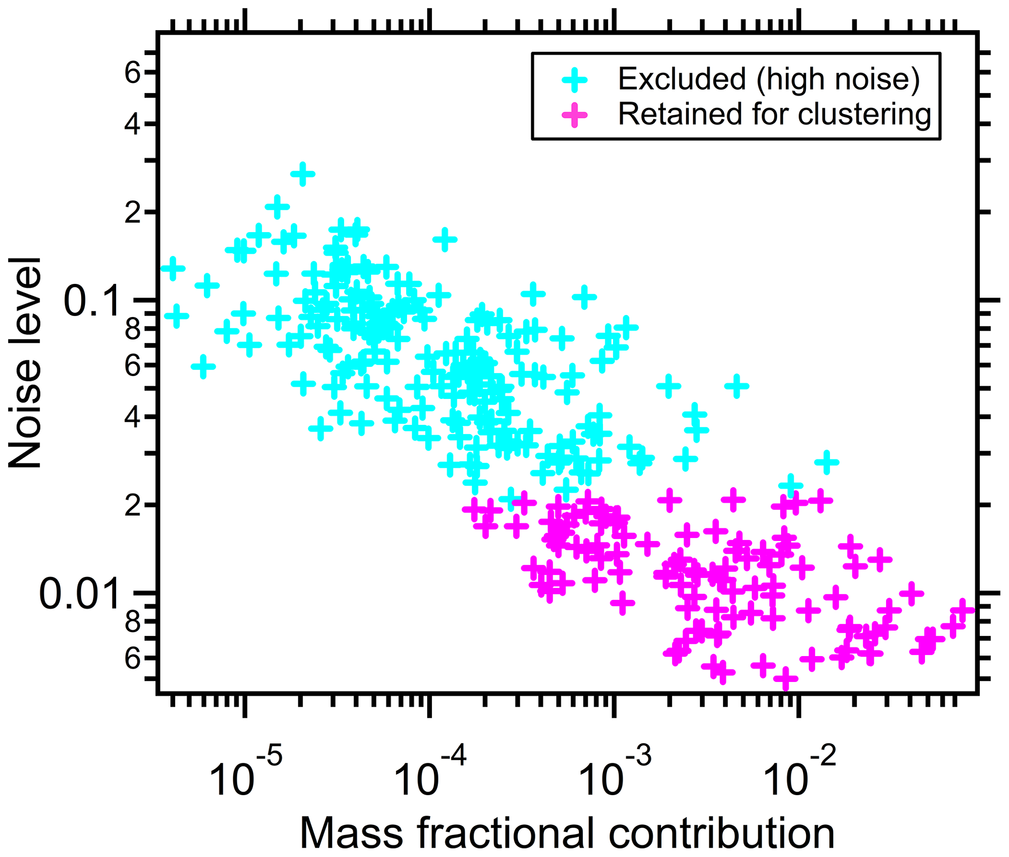
Figure 1The relationship between thermogram noise levels and the fractional contributions of the corresponding ions to total mass for α-pinene + OH SOA. The noise threshold, ξref=0.021, is used to distinguish high-noise thermograms (cyan markers) from thermograms having acceptable noise levels (pink markers).
Table 1Details of SOA formation and chamber conditions for all the example SOA systems.
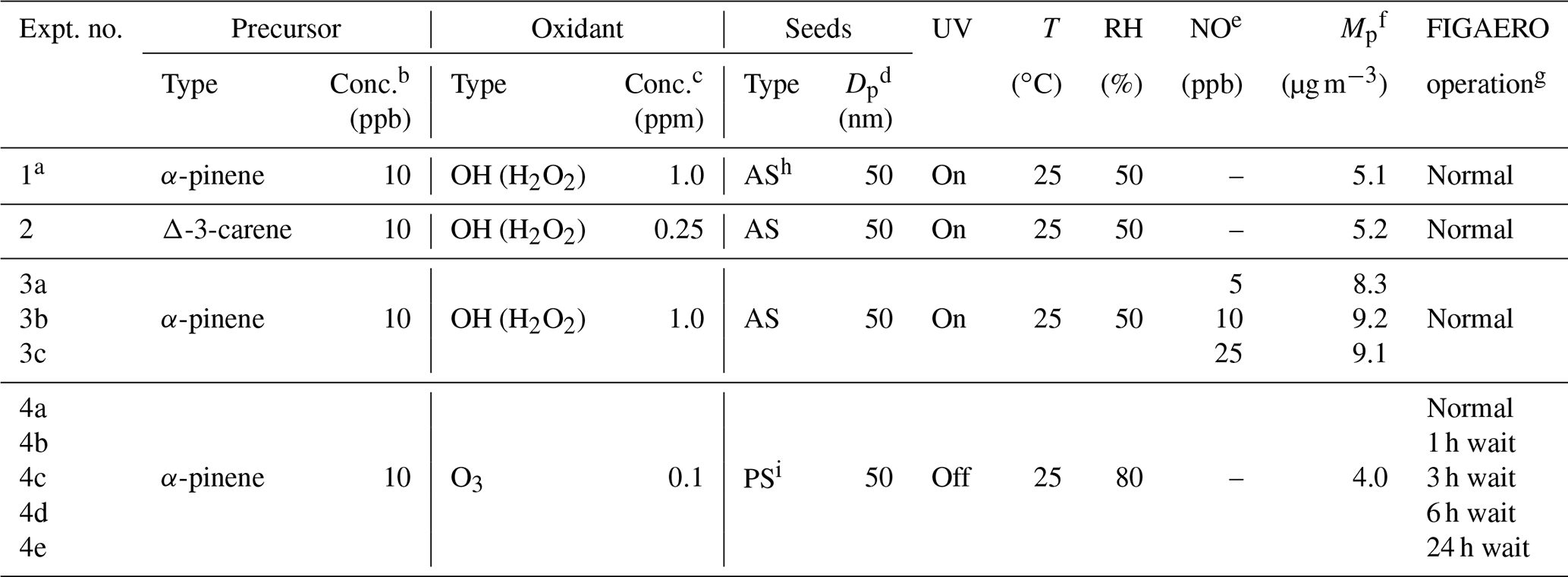
a Experiment no. 1 is a case study used to test the performances of different clustering algorithms. b Conc. of precursors refers to the concentrations expected in the chamber with the absence of any chemistry. c For OH, conc. refers to the concentration of H2O2 injected into the chamber; for O3, conc. refers to the steady-state concentration of O3 in the chamber during SOA formation. d Seed particles are size-selected in all the experiments. e NO concentration refers to the targeted NO concentration when NO is injected into the chamber. The actual steady-state concentration of NO is lower than targeted; “–” indicates that no external NO is added to the chamber. f Mp is the estimated mass concentration of particles including SOA and seeds measured by SMPS when the chamber is at steady state, except for Experiment 4 in which Mp is the mass concentration of SOA only. g Normal operation mode means the desorption process starts immediately after the collection period. X h wait means that particles are isothermally diluted for X h before the desorption process is initiated. h AS: ammonium sulfate. i PS: potassium sulfate.
Discussed further in Sect. 2.3, clustering algorithms often perform poorly when overly noisy data are included in the clustering. This is especially the case for algorithms such as k-means and partitioning around medoids, which assign all the members to a cluster. Clustering methods that do not require the assignment of all members, such as DBSCAN or our NSSC, are generally less sensitive to the influence of overly noisy members. However, we have found that the explicit exclusion of noisy thermograms up front serves to provide for more robust behavior and also removes the need to consider each noisy thermogram as a possible single-member cluster. The inclusion of overly noisy peaks might obscure the underlying structure of clustered thermograms. Noisy thermograms are identified as follows. First, the 5 % of ions having the lowest noise are identified. The ξ value of the noisiest ion from this subset of low-noise ions is defined as the reference noise level, ξref. Small differences in the choice of this threshold (e.g., using the lowest 7 % of ions) do not materially influence the results. Ions for which are considered noisy and excluded from the initial clustering. For the experiments we examined, there are 88–120 out of ∼300 ions left after noise screening, contributing 83.5 %–92.5 % to the total particle mass.
2.2 Noise-sorted scanning clustering (NSSC)
2.2.1 Algorithm description
The noise-sorted scanning clustering (NSSC) algorithm developed here is a variant of the commonly used DBSCAN. In NSSC, the identification and clustering of thermograms occur based on their similarity to seed thermograms. When the ED between a given thermogram and the seed is less than a specified ED criterion (ε) the two members belong to the same cluster. Importantly, in NSSC the selection of the seed thermograms occurs based on their respective noise levels. The least noisy thermogram is selected as the initial seed, the next noisiest is selected as the second seed (assuming it is not already clustered), and so on. We have found that low-noise thermograms typically have more well-defined and characteristic shapes and comprise a substantial fraction of the total mass. The choice to select seeds based on the noise level leads to overall more robust and reproducible clustering compared to the random selection of seeds.
The optimal value of the distance criterion, ε, is not known a priori but must be determined by the user, as discussed in Sect. 2.2.3. A valid cluster must contain at least Nmin members, inclusive of the seed. We use . The consideration and inspection of individual unclustered thermograms exhibiting unique behavior occur as a post-clustering process (Sect. 2.2.2).
The flow of the noise-sorted scanning clustering algorithm is shown in Fig. 2 and summarized here. Clustering proceeds in two rounds. For the initial round, the thermograms are sorted by the noise (ξ), and the ED values between all pairs of thermograms are calculated accordingly. All of the thermograms are identified according to whether they have already been used as seeds (SEED = 0 or 1, with 1 for thermograms used as seeds) and whether they have already been included in a cluster (CLUSTER = 0 or 1, with 1 for already clustered thermograms). At the start, SEED = 0 and CLUSTER = 0 for all thermograms. Clustering begins using the least noisy thermogram having SEED = 0 and CLUSTER = 0 as the initial seed. The state of that seed is then changed to SEED = 1. All thermograms having ED < ε for that seed and with CLUSTER = 0 are identified from the ED matrix; these thermograms are considered neighbors of the seed thermogram. The seed does not evolve as neighbors are added to the cluster during this step. If the number of neighbors plus the seed is greater than or equal to Nmin, the cluster is valid and stored, with the states of all the thermograms in the cluster changed to CLUSTER = 1. Otherwise, the cluster is dismissed, and CLUSTER = 0 for all the members. In this case, the current seed (with SEED = 1 and CLUSTER = 0) will no longer be used as a seed in the future steps but can still end up clustered as a neighbor in the other clusters. The above steps are repeated until all the thermograms have either SEED = 1 or CLUSTER = 1.

Figure 2Flow of the noise-sorted scanning clustering. There are two rounds of clustering. (a) Round 1: the EDs between all thermogram pairs are calculated and two parameters, ε and Nmin, are set. Each thermogram is initialized with state SEED = 0 and CLUSTER = 0. Only thermograms with SEED = 0 and CLUSTER = 0 can serve as seeds, while thermograms with CLUSTER = 0 can be added to new clusters. The procedure terminates when all the thermograms are marked either SEED = 1 or CLUSTER = 1. (b) Round 2: seeds are specified as the weighted average thermogram for each cluster, and any remaining unclustered thermograms from Round 1 are potentially added to these clusters. With the indexing, j refers to the total number of thermograms, i to the number of clusters, and k to the number of unclustered thermograms after Round 1.
Because a cluster must have at least Nmin elements, not all the thermograms may end up clustered. Some of these unclustered thermograms may nonetheless have very similar shapes to the clustered thermograms. Here, an iterative second round of clustering potentially adds these initially unclustered thermograms to the initial clusters using the signal-weighted average thermograms for the clusters from the first round as the initial seeds. A matrix of ED values is calculated between the individual unclustered thermograms and the new seeds. For each unclustered thermogram, the minimum ED, corresponding to only one of the seeds, is identified. When this minimum ED is less than ε, the unclustered thermogram is added into that cluster. A new signal-weighted average thermogram for the cluster is calculated and this process repeats until no additional unclustered thermograms can be added to existing clusters. The mass contribution of the remaining unique unclustered thermograms after this second round can be substantial or negligible, ranging from <0.05 % to 2.6 % in the experiments presented here, and depends largely on the choice of ε. Some of these unclustered thermograms are defined as additional one-member clusters, as discussed in the following section.
2.2.2 Post-clustering processes
After thermograms are clustered, we perform two post-clustering analyses to better understand the whole dataset: (1) identifying additional one-member clusters and (2) sorting of the clusters.
Some of the remaining unclustered thermograms have significant individual mass contributions and should be considered one-member clusters. The criterion of “significant” mass contribution is user-defined. We recommend determining the significance criterion as follows: (i) sorting all the ions (before the noise-filtering process) from largest to smallest individual mass concentration; (ii) calculating the cumulative mass fraction for this sorted list; and (iii) defining as “significant” all those ions contributing to a cumulative mass contribution up to 80 %.
The number of significant ions in a dataset depends on the specific chemical system, varying from only a few to tens of ions. Significant unclustered ions are identified as additional one-member clusters. In some cases, the thermograms for these one-member clusters are unique compared to the previously identified clusters. In others, their shapes are visually similar to the previously identified clusters but with the one-member clusters sufficiently distinct that they were not clustered. For the purpose of automation, these one-member clusters are all included in the final clustering results, and the number of one-member clusters serves as one of the parameters to determine the optimal ε. Users can also choose to exclude them or some of them manually from the final clustering results based on their judgement. For the example systems considered in Sect. 4, there are only a few one-member clusters (ranging from 0 to 4) for the optimal ε used.
Sorting clustered thermograms facilitates the visual presentation and identification of the similarities and dissimilarities among the clusters. The specific method of sorting can be varied depending on the application and system under consideration. Here, we use the temperature at which 50 % of the mass is desorbed (Tm,50) for the weighted average cluster thermogram as a first criterion. The Tm,50 is typically similar to but slightly larger than the temperature at which the signal reaches a maximum. As such, the Tm,50 is approximately related to the saturation vapor pressure of the desorbing compound, at least for compounds that desorb directly (e.g., Lopez-Hilfiker et al., 2014). When two or more clustered average thermograms have identical Tm,50, a rare but occasional occurrence, they are further sorted by Tm,75, the temperature at which 75 % of the mass is desorbed. The temperature difference between Tm,50 and Tm,75 indicates the slope of the thermogram between these two temperatures, with larger values indicating slower decay. Therefore, these two parameters generally illustrate the shape of a thermogram. The Tm,50 and Tm,75 are determined by calculating the cumulative desorbed mass and finding the temperatures at which 50 % and 75 % are reached.
The sorting process tends to organize the cluster-specific thermograms such that clusters having lower peak temperatures (lower Tm,50) and steeper downslopes after the peak (lower Tm,75) come first. Thermograms of this type are indicative of major contributions from higher-volatility monomers (Schobesberger et al., 2018). Thermograms having higher Tm,50 generally have broader peaks and shallower downslopes, indicative of substantial contributions from low-volatility compounds or the decomposition of oligomers. A further discussion of the interpretation of thermogram shapes is provided in Sect. 3.2.
2.2.3 Choosing the optimal ε
NSSC is a distance-based clustering method, so the choice of the distance criterion, ε, is a crucial step. For small ε, members within a cluster have high similarity, but few thermograms end up clustered. In contrast, for large ε the majority of the thermograms are clustered into only a few clusters having comparably low intra-cluster similarity. The choice of the optimal ε value is guided here by the consideration of several parameters that vary with ε. The overall aim is to simultaneously (i) minimize the unclustered mass fraction (fm,unclustered) while (ii) maximizing the number of clusters (Nc) having two or more members and (iii) minimizing the number of one-member clusters (Nc,one) yet (iv) maintaining inter-cluster separation (RinterClst).
In general, Nc increases with ε for small ε because more thermograms of different shapes get clustered and fewer thermograms remain unclustered. As ε further increases, some clusters are combined and a greater number of thermograms are assigned to a single cluster. Consequently, as ε increases the Nc generally increases, reaches a maximum level, and then decreases. The maximum Nc and the ε at which the maximum occurs depend on the exact size and the properties of the dataset being examined. We have found that a typical SOA system usually has 9–13 distinct thermogram clusters. We recommend selecting an ε that provides for Nc at or near the maximum as this captures the greatest number of thermogram types.
The mass fraction of unclustered thermograms, fm,unclustered, includes only the unclustered thermograms that were not excluded based on the noise filtering. In general, a smaller fm,unclustered is preferable as this indicates that a greater amount of the OA mass is included in a cluster (including one-member clusters). The fm,unclustered generally decreases with ε, then plateaus above a certain value of ε; ideally this plateau occurs at . The ε where the plateau starts is indicated as εMF, where MF stands for mass fraction. Given that significant one-member clusters are allowed, the unclustered thermograms that remain above εMF have individually small mass contributions and are either truly unique in their shapes or have a sufficiently high noise level that they cannot be clustered, even after the noise-screening process. We generally recommend selecting ε≥εMF to minimize the unclustered mass.
The number of one-member clusters, Nc,one, generally decreases with ε, as these ions are incorporated into multi-member clusters. Ideally, these one-member clusters would exhibit clear, visually distinct behavior compared to other one-member clusters and to multi-member clusters. However, we find this is often not the case, especially at smaller ε. Thus, the number of one-member clusters should generally be minimized; we suggest Nc,one be held to 5 or fewer in general.
The inter-cluster separation parameter, RinterClst, characterizes the dissimilarity between clusters and is the ratio between the average inter-cluster distance (EDseed,avg) and ε, where
and ED is the distance between the seeds for the different clusters i and j and . For a 2-D dataset, the seed can be visualized as the center of a circle and ε the radius of the circle. Thus, when ED, the two circles defining the boundaries of these two clusters have overlapping areas. Good separation (i.e., cluster dissimilarity) is indicated when ED. Although our dataset is more than two dimensions, this illustrates the idea of establishing the level of similarity (or dissimilarity) between clusters, i.e., the extent to which they are unique. We recommend selecting an ε that results in RinterClst≥2, when possible.
All four parameters should be considered when determining the optimal ε. Consideration of the parameters individually may not result in the same optimal ε. Ultimately, the user must consider each parameter and aim to select an optimal ε that balances the different information provided in each parameter. This can be achieved by plotting the above parameters as a function of ε and then selecting as the optimal value the ε that results in (i) a small fm,unclustered with (ii) Nc near the maximum and (iii) a small Nc,one and (iv) RinterClst near or above 2. In addition, visual comparison of the clustering results, illustrated as the average thermogram of each cluster, can be helpful. For the example data considered below, we find that the optimal ε tends to fall within a relatively narrow range of values.
2.2.4 Summary
The NSSC allows for the clustering of ion peaks in temperature-dependent mass spectra measured by FIGAERO-CIMS, from which mass thermograms of the different clusters are determined. The NSSC emphasizes the contributions of ions having high a signal-to-noise ratio by selecting seeds for the mass spectral clusters according to a decreasing signal-to-noise ratio. The NSSC also accounts for the full temperature-dependent behavior of each ion, weighted towards the temperature ramping period during which the ions generally exhibit more characteristic desorption profiles. However, the NSSC requires as user input a distance criterion, ε, which characterizes the minimum similarity required between a selected seed ion thermogram and all other (non-clustered) ion-specific thermograms for the non-seed ion to be considered part of the mass spectral cluster. The appropriate ε value must be uniquely determined for a given experiment or set of experiments, but we recommend that it should be selected to provide both the greatest amount of clustered mass and the number of mass spectral clusters having two or more members while also maintaining the greatest average separation between the mass spectral clusters. Altogether, these steps facilitate a robust, reproducible determination of mass spectral clusters from a given dataset.
2.3 Alternative clustering methods
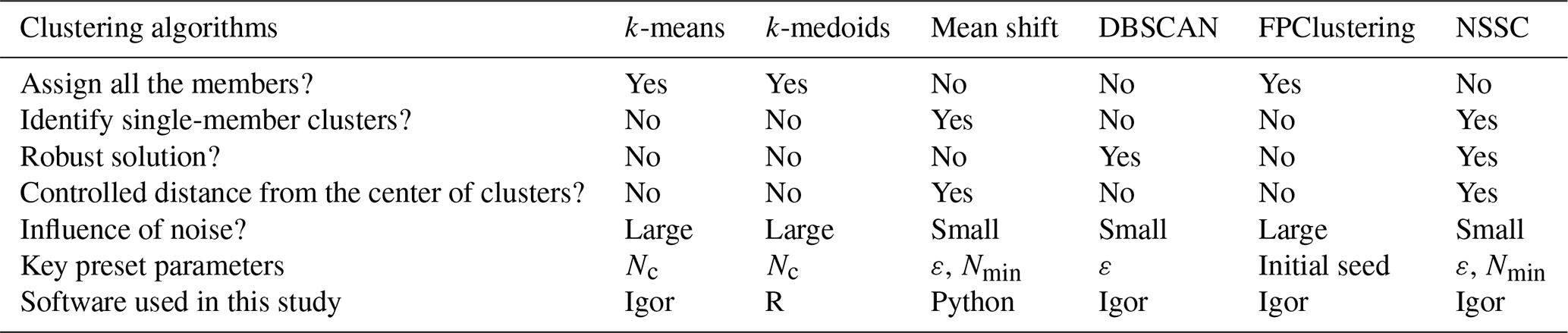
We have alternatively considered the performance of some of the most commonly used clustering algorithms (k-means, k-medoids, mean shift, DBSCAN) and a less commonly used one (FPClustering; Gonzalez, 1985) for interpreting FIGAERO-CIMS observations. The clustering methods considered are summarized in Table 2, with some of their pros and cons listed, and described in further detail in Appendix A. We discuss them briefly here in the context of FIGAERO-CIMS data. All the methods considered require the input of at least one key user-specified parameter. These parameters and the associated clustering algorithms can be generally classified into two categories: number-based and distance-based. Number-based clustering algorithms require the specification of the desired number of retrieved clusters; this includes k-means and k-medoids. Number-based algorithms usually assign all members to clusters. The extent of similarity among members of a cluster can vary greatly since there is no strict distance criterion for each cluster. When applied to FIGAERO-CIMS thermograms, we have found these number-based algorithms are particularly sensitive to the presence of noisy members and the initialization method. In contrast, some clustering algorithms require the specification of a distance (similarity) criterion. This includes the mean shift, DBSCAN, and our NSSC algorithm. These distance-based algorithms need not cluster all members of the initial population and generally emphasize intra-cluster similarity or the density of the points. The methods differ in terms of the procedure used for the selection of the initial seed or center and the extent to which they emphasize point density versus cluster similarity. Noisy members tend to naturally be excluded from any clusters. NSSC is a variant of DBSCAN. It does, however, differ from the standard DBSCAN algorithm because NSSC only searches for neighbors of the seed, while DBSCAN also searches for neighbors of the neighbors. In doing so, NSSC emphasizes cluster similarity rather than point density. This is particularly useful when clustering thermograms, as the behavior of the entire thermogram is considered; inclusion of neighbors of neighbors may cluster together thermograms that exhibit especially similar behavior in one region (e.g., the soaking period) but not another, an undesirable result. Accordingly, the sorting of seeds by noise levels is a key aspect of the NSSC algorithm, which we have found provides for more robust clustering results.
Most of these clustering algorithms, including k-means, k-medoids, and mean shift, are initialized with a random choice of the initial cluster centers (or seeds). For large datasets, this randomness usually leads to different results of clustering with different runs. The extent to which this impacts the analysis and clustering of FIGAERO-CIMS data is considered using SOA from the α-pinene + OH SOA system as the case study (Sect. 4.1). For the FIGAERO-CIMS data we find that the various clustering results exhibit a moderate sensitivity to how the initial seeds are selected for all of these algorithms, although the final clusters are generally similar between different runs for the same input parameter. This may reflect either the relatively small size of the dataset (∼300 members originally and ∼100 members after noise screening) or that there are generally characteristic peak shapes with overall good separation. However, some differences between independent clustering runs result, which is undesirable. For FIGAERO-CIMS data we know that not all thermograms are of equal quality; i.e., they have different noise levels reflecting in part their different overall contributions to the total mass. The standard clustering methods do not account for this information. The NSSC algorithm developed here takes into account this measure of data quality and uses it to identify the seeds for clustering. This provides for an entirely reproducible clustering and generally emphasizes the behavior of the ions that contribute most to the FIGAERO-CIMS signal while still allowing for the consideration of the contributions of low-signal ions.
We find that different clustering algorithms can result in similar numbers of clusters, with the cluster-averaged thermograms having visually similar shapes when each is run with appropriate user-selected parameters, although the details and robustness of each cluster vary method by method. The “appropriate” parameters, however, are different from the “optimal” parameters. There is usually different guidance for different algorithms on how to find the optimal parameters that result in the greatest similarity within clusters and dissimilarity among clusters. In the case of k-medoids, for example, the average silhouette indicates an optimal number of clusters of two for the case study system. Yet, this is certainly too few clusters based on the other methods.
In summary, we propose NSSC as the preferred algorithm in dealing with the FIGAERO dataset based on the following: (i) the ability to generate similar results as the other commonly used clustering algorithms; (ii) good reproducibility and stability of results due to accounting for the noise of individual thermograms; (iii) good control over the similarity within the clusters by using a user-definable distance criterion; and (iv) a capability to identify unique thermograms as one-member clusters.
3.1 Instrument and experiment description
The FIGAERO-CIMS instrument has been described previously in detail (Lee et al., 2014; Lopez-Hilfiker et al., 2014). A brief description is provided here, with some additional details in the Supplement. FIGAERO-CIMS measures the evolved gases from filter-collected particles during temperature-programmed thermal desorption. The thermal desorption of particles occurs in two stages: a ramping period and a soaking period. During ramping, the temperature increases from room temperature to 200 ∘C, typically at 10 ∘C min−1. Most OA mass desorbs during the ramping stage. The temperature is held at 200 ∘C for ca. 30–40 min during the soaking period to facilitate evaporation of the remaining low-volatility organic mass from the filter. The evolved gas-phase compounds are measured using CIMS with the iodide (I−) reagent ion, appropriate for the characterization of generally highly oxygenated components comprising most secondary organic aerosol (Lopez-Hilfiker et al., 2016; Isaacman-VanWertz et al., 2017; Lee et al., 2018). The resulting signal or mass concentration versus temperature (or equivalently time) curves for each ion constitute a thermogram. All individual thermograms are background-corrected by subtracting the observed thermograms from appropriate blank experiments. The overall bulk thermogram is obtained by summing together the individual thermograms.
Several example applications of the clustering on FIGAERO-CIMS data are discussed in Sect. 4. These cover laboratory experiments on SOA derived from the following: (1) OH+α-pinene and (2) OH+Δ-3-carene, both at low NOx conditions; (3) OH+α-pinene as a function of [NO]; and (4) O3+α-pinene, but with the SOA allowed to isothermally evaporate at 80 % RH for varying amounts of time prior to thermal desorption. These experiments are summarized in Table 1, with further details in the Supplement and associated publications (D'Ambro et al., 2018, 2019); all data are publicly available (Cappa et al., 2019). All the experiments were done in a 10.6 m3 Teflon environmental chamber at Pacific Northwest National Laboratory (PNNL) (Liu et al., 2012, 2016).
3.2 General interpretation of FIGAERO-CIMS thermograms
This work focuses on the development of the clustering method rather than on interpretation of the FIGAERO-CIMS thermograms; an illustrative thermogram is shown in Fig. 3b. However, a discussion of the clustering results is aided by a general understanding of how FIGAERO-CIMS thermograms have been previously interpreted. Ions contributed by semi-volatile and low-volatility compounds that desorb directly tend to exhibit strongly peaked, Gaussian-like thermograms with single-mode peaks of around 50 to 120 ∘C; the lower the peak desorption temperature (Tpeak) the higher the volatility of the desorbing compound (Lopez-Hilfiker et al., 2014, 2015). We therefore refer to thermograms, or portions of thermograms, having this general shape as the “monomeric” content of the ion hereafter; direct evaporation of thermally stable dimers or other oligomers is possible, although it will typically occur at higher temperatures due to the comparably lower volatility of these compounds. When multiple monomeric compounds having different vapor pressures contribute to the same ion, the resulting thermogram exhibits a broader peak and shallower slopes or, in particular cases, multiple distinct peaks (Lopez-Hilfiker et al., 2015). However, very broad thermograms, especially those that peak at higher temperatures (> 120 ∘C or so), can also indicate contributions from the thermal decomposition of very low-volatility monomers, dimers, and oligomers (Lopez-Hilfiker et al., 2015; Gaston et al., 2016; Schobesberger et al., 2018). Dimers and oligomers can evaporate directly, without thermal decomposition, as observed for isoprene-derived SOA (D'Ambro et al., 2017) and ambient monoterpene oxidation products (Mohr et al., 2017). However, fragments of dimers or oligomers are generally more abundant, indicating the importance of thermal decomposition for the desorption of these low-volatility compounds. Both the direct evaporation of extremely low-volatility compounds and the decomposition of large molecules or oligomers can lead to high signal levels above ∼120 ∘C. We refer to both peaks and the slowly varying signal above ∼120 ∘C as the “oligomeric” content of the ion hereafter. We use the terms monomer and oligomer in a qualitative manner. A more quantitative analysis of the thermograms can help distinguish between direct evaporation, thermal decomposition, and the contributions of monomers versus oligomers (Schobesberger et al., 2018), yet this is beyond the scope of the current work.
To illustrate the broad utility of NSSC for the interpretation and analysis of FIGAERO-CIMS data, we apply NSSC to the laboratory-generated SOA systems described above. The systems include SOA formed from a single precursor under NOx-free conditions, SOA formed from a single precursor as a function of input [NO], and SOA formed from a single precursor with thermal desorption following isothermal evaporation.
4.1 α-pinene + OH SOA
A total of 298 ions were characterized by FIGAERO-CIMS for SOA generated from the α-pinene + OH reaction (Table 1). Four ions were characterized as anomalous and excluded from further analysis (see Sect. 2.1.1). The mass concentration of each ion was calculated by integrating the signal across the entire desorption period and assuming an equal sensitivity of CIMS for all the compounds. The total mass concentration is the sum of all the non-anomalous ions. The mass spectrum and bulk thermogram of the remaining 294 ions are shown in Fig. 3, with the bulk thermogram shown versus both temperature (Fig. 3b) and time (Fig. 3c) to illustrate the difference between the ramping and soaking periods. The individual thermograms exhibited a variety of shapes. The noise threshold for this dataset was ξref=0.020893. A total of 188 ions were screened out via noise filtering. The remaining 106 ions contribute 92.5 % to the total mass detected by FIGAERO-CIMS. The optimal ε was established through consideration of the codependencies of Nc, Nc,total, fm,unclustered, and RinterClst on ε (Fig. 4; Table 3). For this dataset, we determine the optimal ε=2.6. The choice of a much smaller ε, around 1.5, gives a maximum in Nc but leaves a large fraction of the mass unclustered. The choice of ε=2.1 or 2.2 yields larger Nc and RinterClst than ε=2.6, with a reasonably small fm,unclustered. However, there is one type of thermogram (Clst no. 11 in Fig. 5) that is only captured with ε≥2.6, and this yields . Using ε≥2.7 also yields and , but Nc and RinterClst decrease from ε=2.6, indicating increasing similarity between clusters with fewer types of shapes captured. The choice of ε=2.6 provides a compromise between maximizing Nc, minimizing fm,unclustered, and keeping RinterClst above 2. The parameters and thresholds used for this dataset are summarized in Table 3.

Figure 3(a) Mass spectrum of α-pinene + OH SOA measured by FIGAERO-CIMS. The mass excludes iodine. (b) Normalized thermogram of the bulk SOA versus temperature. (c) Normalized thermogram of the bulk SOA versus time (black line) and the variation in desorption temperature with time (dark red dashed line). The long tail during the soaking period is evident when the thermogram is considered in time space. The light blue shaded area denotes the ramping period and the pink shaded area the soaking period.
Table 3Parameters and thresholds used for the data processing and noise-sorted scanning clustering for all the example experiments.
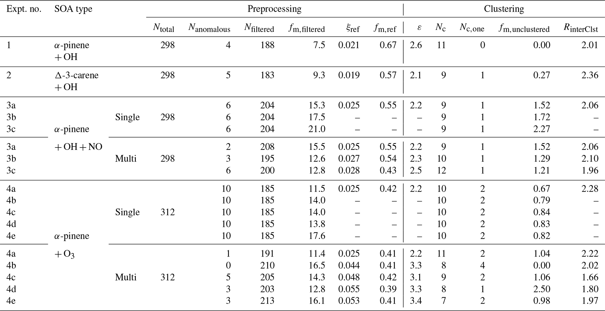
Ntotal – total number of ions characterized by CIMS. Nanomalous – number of anomalous ions. Nfiltered – number of ions filtered out from the following clustering due to high levels of noises. fm,filtered – mass fraction of the ions filtered out due to high levels of noises, expressed in percent. ξref – noise threshold. Ions with noise levels above this threshold are excluded from clustering. fm,ref – the threshold of mass contribution (%) to identify an ion as significant. ε – distance criterion. Nc – number of clusters determined with two or more members. Nc,one – number of clusters determined with only one member. fm,unclustered – mass fraction of unclustered ions, expressed in percent. RinterClst – the ratio of the average inter-cluster distance over the distance criterion ε.
A total of 11 clusters are identified with no one-member clusters. The unweighted and mass-weighted average thermograms for each cluster are shown along with the thermograms of individual members in Fig. 5a. The differences between weighted and unweighted average clusters are negligible, in general. Clusters are organized and numbered (as Clst no. N) from low to high Tm,50, with deeper to shallower downslope. Clst no. 1 through Clst no. 6 all have a clear peak below 120 ∘C, but with different peak widths and downslopes. Clst no. 7 and Clst no. 8 are a bit noisier with only a few members each, exhibiting a sharp upslope and shallow downslope. Clst no. 9 has a very broad peak. Clst no. 10 peaks at around 150 ∘C after an initial rise and temporary plateau. Clst no. 11 exhibits behavior somewhat like Clst no. 10, but with a peak that occurs just into the soaking period, evident if viewed in time space, at 200 ∘C with a rapid drop afterwards.
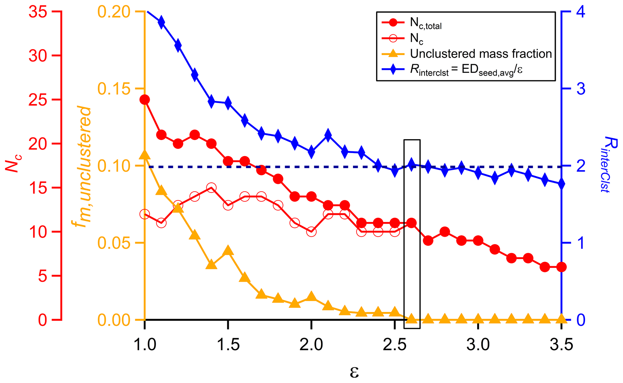
Figure 4The variation of four parameters, Nc, Nc,total, fm,unclustered, and RinterClst, as a function of the distance criterion ε. The black horizontal dashed line guides the judgement for RinterClst≥2. The values highlighted by a rectangle are the values corresponding to the optimal ε used for the clustering analysis.
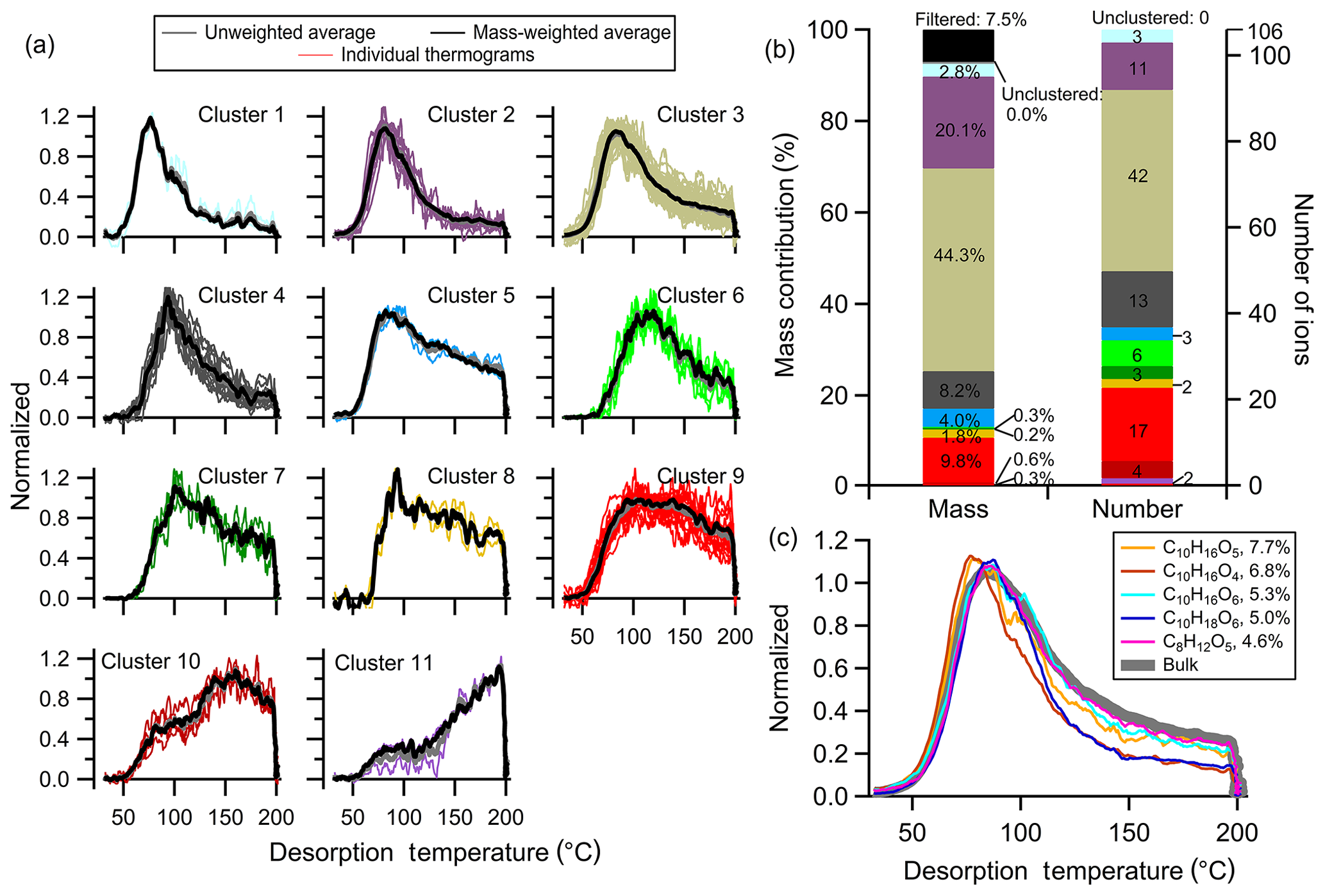
Figure 5Clustering results for α-pinene + OH SOA. (a) Unweighted average thermograms (bold gray lines), mass-weighted average thermograms (bold black lines), and individual members (colored lines) of the 11 clusters identified. (b) Percentage contribution of each cluster to the total mass, the filtered-out and unclustered mass percentage (left bar), the number of ions in each cluster, and the unclustered number of ions (right bar). (c) Thermograms of the top five ions in terms of mass contribution. The cluster colors are consistent between (a) and (b).
The total mass concentration of a given cluster (Mc,N) is the sum across all cluster members, calculated by integrating the summed mass concentration across the entire desorption period. The percentage mass contribution of each cluster and of the unclustered and the noise-filtered ions, as well as the number of members for each cluster, are shown in Fig. 5b and Table S1 in the Supplement. Clst no. 2 and Clst no. 3 contain the majority of the mass (20.1 % and 44.3 %, respectively) and consist of nearly half of the clustered ions (11 and 42, respectively). Clst no. 4 and Clst no. 9 also contain a notable percentage of the total mass (8.2 % and 9.8 %, respectively) and include a notable number of ions (13 and 17, respectively). Other clusters contribute relatively little to the total mass and contain a small fraction of ions.
The mass-weighted average molecular formulas (CxHyOzNm) differ between clusters, as do the O : C and H : C atomic ratios (Table S1). There is no clear relationship between Tm,50 (or cluster number) and the number of carbon atoms, MW, or O : C. There is, however, a reasonable inverse correlation between Tm,50 and H : C (r2=0.78). The number of carbon atoms is notably larger for Cluster 6 (x=11.1) and Cluster 7 (x=15.3); if those two clusters are excluded there is an inverse relationship between Tm,50 and the number of carbon atoms (r2=0.79) and with MW (r2=0.59). While the reason for these two clusters having comparably large numbers of carbon atoms is unknown, this nonetheless suggests that the contribution of oligomer decomposition might increase for clusters having higher Tm,50 values.
Interpretations of previous FIGAERO-CIMS studies have largely focused on the behavior of the bulk thermogram or of several major ions or sums of ions based on common factors such as the number of carbon atoms (Lopez-Hilfiker et al., 2016; D'Ambro et al., 2017, 2018; Stolzenburg et al., 2018; Wang and Hildebrandt Ruiz, 2018; Joo et al., 2019). The normalized thermograms of the top five ions contributing most to the total mass for the experiments here are shown in Fig. 5c, along with the bulk thermogram. Together, these five ions make up nearly 30 % of the total mass, exhibit very similar thermogram shapes to each other and to the bulk thermogram, and belong solely to either Clst no. 2 or Clst no. 3. Thus, examining these ions only would capture only a fraction of the overall diversity in thermal behaviors. The clustering method developed here provides a means to more comprehensively investigate the variability in volatility between aerosol components.
4.2 Δ-3-carene + OH SOA
A total of 298 ions were characterized by FIGAERO-CIMS for SOA generated from the reaction of Δ-3-carene + OH (Table 1). Five were identified as having anomalous thermograms and excluded from further analysis. The mass spectrum and bulk thermograms of Δ-3-carene + OH SOA are shown in Fig. 6. Compared to the α-pinene + OH SOA described above, the mass spectrum of Δ-3-carene SOA is quite different, with one ion (C8H12O5) dominant. The bulk thermograms of the two SOA systems both look bell-like, but with the Δ-3-carene SOA thermogram having a peak temperature ca. 9 ∘C higher. After noise filtering, 110 ions remained for clustering, contributing 90.7 % to the total mass. The optimal ε is 2.1, established again by considering the system-specific dependence of Nc, Nc,one, fm,unclustered, and RinterClst on ε (Fig. S1 in the Supplement), with the parameters and thresholds summarized in Table 3.

Figure 6Same as Fig. 3, but for Δ-3-carene + OH SOA. (a) SOA mass spectrum measured by FIGAERO-CIMS. The mass excludes iodine. The normalized thermogram of the bulk SOA versus (b) temperature and (c) time. In (c) the light blue shaded area denotes the ramping period and the pink shaded area the soaking period.
A total of 10 clusters are identified, including one one-member cluster, with thermograms shown in Fig. 7a and the mass contribution and number of ions in a cluster in Fig. 7b. The chemical properties of each cluster are summarized in Table S2. The general characteristics of the thermograms identified in Δ-3-carene + OH SOA are similar to those of the low NOx α-pinene + OH SOA described above but with different mass contributions. For example, Clst no. 4 has a nearly identical shape of the thermogram as Clst no. 3 in the α-pinene SOA but contributes less to the total mass: 28.0 % compared to 44.3 %. Clst no. 6 in the Δ-3-carene SOA contributes 14.8 % to the total mass and resembles Clst no. 5 in the α-pinene SOA, which contributes only 4.0 % to the total mass.
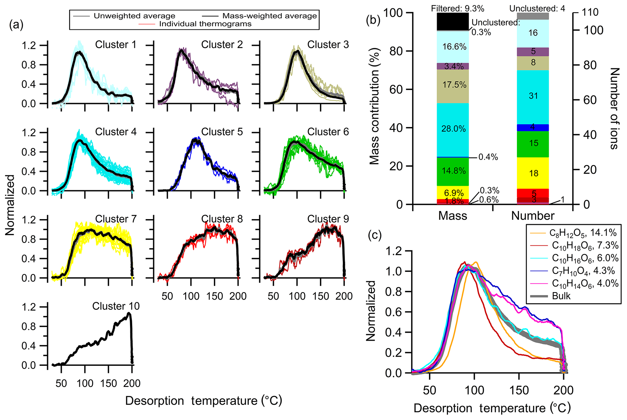
Figure 7Same as Fig. 5, but for Δ-3-carene + OH SOA. (a) Unweighted average thermograms (bold gray lines), mass-weighted average thermograms (bold black lines), and individual members (colored lines) of the 10 clusters identified. (b) Percentage contribution of each cluster to the total mass, the filtered-out and unclustered mass percentage (left bar), the number of ions in each cluster, and the unclustered number of ions (right bar). (c) Thermograms of the top five ions in terms of mass contribution. The cluster colors are consistent between (a) and (b).
In general, Clst nos. 1–6 in the Δ-3-carene SOA all exhibit a peak below 120 ∘C, with clear peaks of varying width and downslopes of varying steepness, but nominally in order of narrow to wide and steep to shallow, respectively. These clusters carry the majority of the desorbed mass. Clst no. 7 and Clst no. 8 both exhibit relatively flat thermograms in the ramping period after their initial rise and contribute 9 % to the total mass. Clst no. 9 has a peak temperature above 150 ∘C and Clst no. 10 reaches a maximum during the soaking period. These last two clusters contribute little to the total mass (0.6 % and 0.3 %, respectively).
The thermograms of the five largest ions are shown in Fig. 7c. These five ions together carry ∼35 % of the SOA mass. A wider variety of thermogram shapes is captured by the top five ions compared to the α-pinene SOA system. However, thermograms characteristic of Clst nos. 7–10 are not represented by these top five ions; this remains true even if the top 10 ions are considered (not shown).
There are ultimately three major differences between the two SOA systems. For one, there is a different relationship between fractional contribution and cluster number (and thus Tm,50) between the two. Secondly, the α-pinene SOA contains ions with especially narrow peaks at ca. 100 ∘C (i.e., Clst nos. 7 and 8) that are not observed with Δ-3-carene SOA (compare Fig. 5 with Fig. 7). Lastly, the thermograms of the top five ions for Δ-3-carene SOA differ to a greater extent than for α-pinene SOA. Although we are unable to determine the reasons for these differences here, this illustrates the potential for clustering to help identify and understand differences between different SOA systems.
4.3 α-pinene + OH + NO SOA
Thermograms from SOA generated from the reaction of α-pinene + OH at varying NO concentrations (5, 10, and 25 ppb; Table 1) are considered as a set of experiments. Together, the differences between them illustrate the impact of changes to the fate of RO2 peroxy radical intermediates on the SOA composition and thermal properties (Praske et al., 2018; Zhao et al., 2018). Clustering proceeds here using two complementary approaches. In the single-clustering method, clustering is performed for one reference experiment (i.e., at one NO concentration, 5 ppb, Expt. no. 3a). Then, average thermograms are calculated for the other experiments in the set using the same cluster members as identified in the reference experiment. In the multiple-clustering method, clusters are independently determined for each experiment in the set, and the shapes, relative abundances, and contributing ions are compared between experiments. For all three experiments, the same initial set of 298 ions were characterized by FIGAERO-CIMS.
4.3.1 Single clustering
The ions identified as anomalous in each experiment differed. This most likely results from shifts in the background signal levels between experiments. To maintain consistency between the three experiments, ions identified as anomalous in any of the experiments were excluded from all the experiments, with four ions excluded in total. A total of 88 ions were kept for clustering after noise filtering using the 5 ppb NO reference experiment, contributing 84.5% to the total mass. The optimal ε is 2.2 (Fig. S2 and Table 3), resulting in 10 clusters with one one-member cluster. The same sets of ions were then used to calculate the cluster-averaged thermograms for the 10 and 25 ppb NO experiments. The chemical characteristics of the clusters are summarized in Table S3.
Mass spectra for the three experiments are compared in Fig. 8a and the bulk thermograms shown in Fig. 8b and c. The 5 and 10 ppb NO SOA mass spectra are nearly identical. The mass spectrum for the 25 ppb NO experiment, however, exhibits a notable shift of the most abundant ions towards lower m∕z. The bulk thermograms for the 5 and 10 ppb NO experiments are nearly identical, peaking near 80 ∘C. The 25 ppb NO bulk thermogram similarly peaks near 80 ∘C but exhibits a much slower decay as temperature increases further. Additionally, the change in slope at the transition from the ramping to soaking period is more pronounced in the 25 ppb NO experiment. Overall, a greater fraction of the mass desorbs above 100 ∘C and during the soaking period for the 25 ppb NO experiment compared to lower-NO experiments.
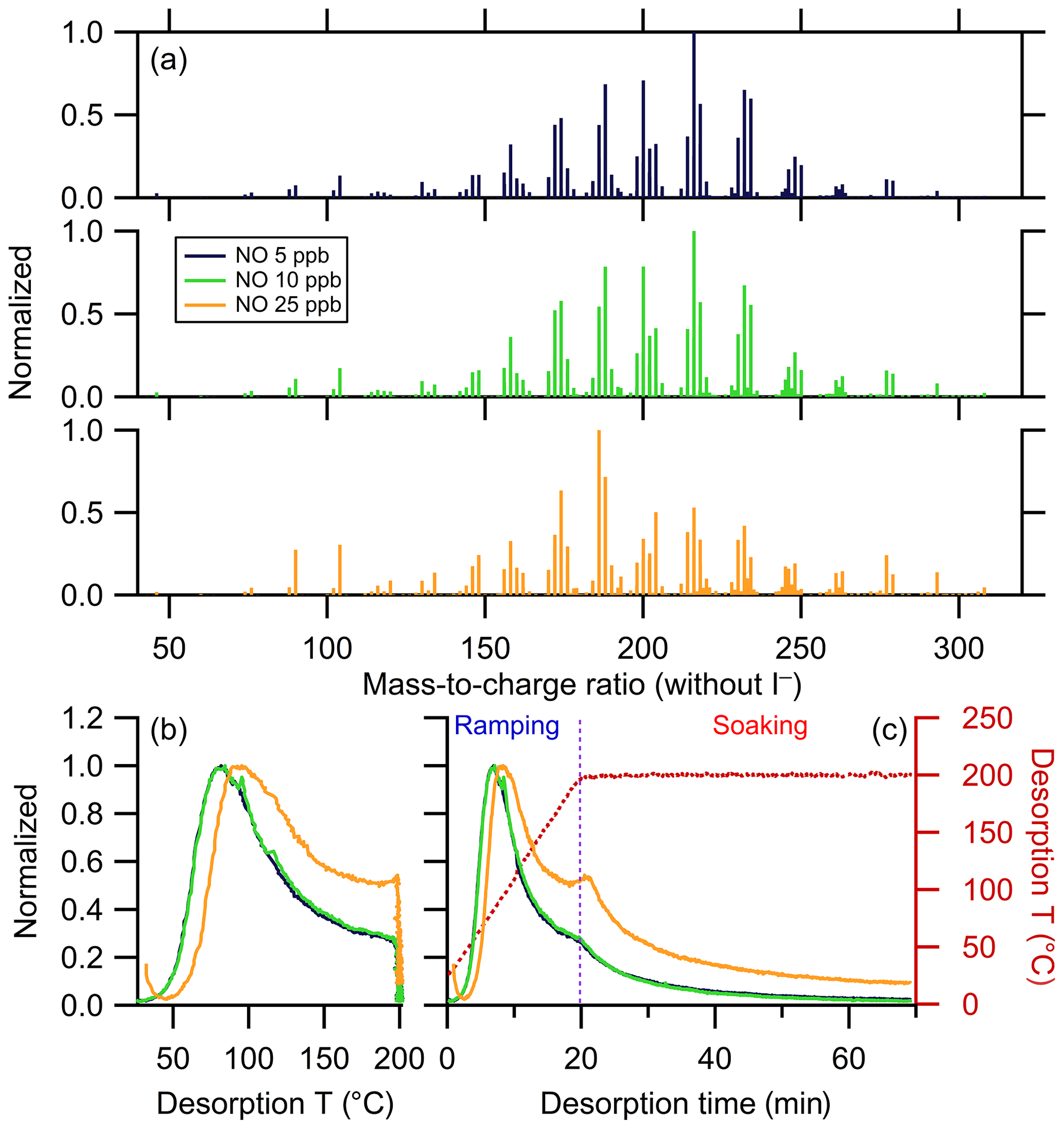
Figure 8(a) Mass spectra of α-pinene + OH SOA formed with different NO concentrations, normalized to the mass concentration of the most abundant ions. The mass excludes iodine. Normalized thermograms of the bulk SOA versus (b) temperature and (c) desorption time, with the desorption temperature shown as a dark red dashed line. The vertical purple dashed line delineates between ramping and soaking. In all the panels, colors correspond to the NO concentration (see legend).
Despite the differences in the bulk thermograms, the shapes of the weighted average thermograms of clusters for all the NO experiments are generally similar, with the exception of Clst no. 6 (Fig. 9a). In particular, the 25 ppb thermogram shape of Clst no. 6 differs substantially from those of low NO conditions, with a much reduced initial peak (around 80 ∘C) and a more pronounced second peak at high temperature (around 200 ∘C). However, this cluster contributes negligibly to the overall mass. There is some suggestion of similar behavior for Clst no. 10, although to a lesser extent. For the three most abundant clusters, Clst nos. 1, 2, and 4, there is a slightly increased relative contribution of the 100–200 ∘C tail for 25 ppb NO, consistent with differences in the bulk thermograms.
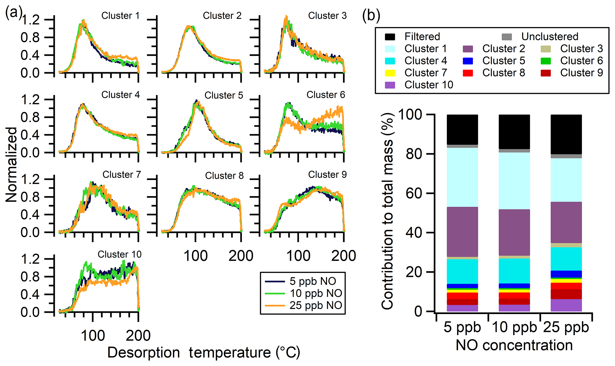
Figure 9Single-clustering results for α-pinene + OH SOA as a function of NO concentration. (a) Comparison of the normalized, weighted average thermograms of the 10 clusters for the 5 ppb NO (navy), 10 ppb NO (green), and 25 ppb NO (orange) experiments. (b) Contribution of each cluster to the total mass, including the contribution from filtered-out ions (black) and unclustered ions (gray). The total mass is calculated independently for each experiment.
The most notable NO-dependent change is in the relative abundances of the clusters between the 5 and 10 ppb NO experiments and the 25 ppb NO experiment (Fig. 9b). The cluster mass fractions are nearly identical between the 5 and 10 ppb NO experiments. The relative contributions of higher-number clusters (which have been ordered according to increasing Tm,50) increase for the 25 ppb NO experiment. This is consistent with the increased persistence of the 25 ppb NO bulk thermogram to higher temperatures and the nearly identical nature of the 5 and 10 ppb NO bulk thermograms (Fig. 8b). The clustering analysis suggests that differences in the bulk thermogram arise from shifts in the relative contributions of the various SOA components that result from the altered photochemical environment. These observations generally suggest an increasing fraction of oligomeric content, or less-volatile compounds, formed in the particle phase – or potentially the gas phase – when the SOA was generated under higher NO chamber conditions (Schobesberger et al., 2018).
4.3.2 Multiple clustering
With multiple clustering, each experiment was processed and clustered independently with experiment-specific ξref, Nc, and ε, among other parameters (Fig. S4 and Table 3). The clustered thermograms from the three experiments are compared in Fig. 10a–c. The number of clusters identified increases with NO concentration. Comparison between the shapes of the clusters from the 5 ppb NO (Fig. 10a) and 10 ppb NO (Fig. 10b) experiments indicates generally similar types of thermograms, consistent with the single-clustering method; 10 of the 11 total 10 ppb clusters match a 5 ppb cluster. The one additional unique cluster at 10 ppb NO (Clst no. 9) is a one-member cluster with a sharp, narrow peak at low temperatures and a broader, shallow second peak at high temperatures. This ion was filtered out due to a high noise level in the 5 ppb NO experiment.
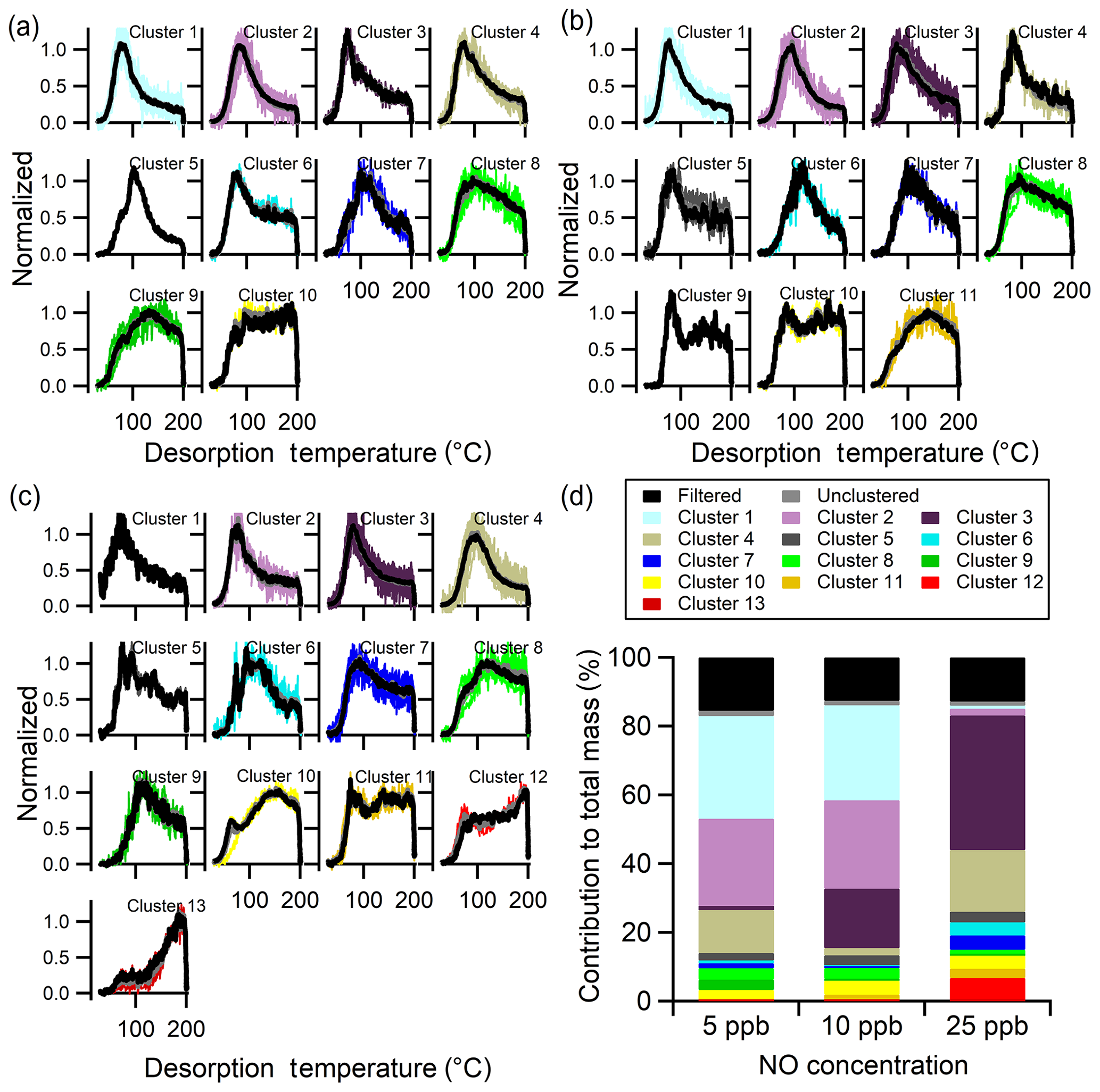
Figure 10Multiple-clustering results for α-pinene + OH SOA as a function of NO concentration. Clustering results are separately shown for the (a) 5 ppb NO, (b) 10 ppb NO, and (c) 25 ppb NO experiments. Each panel includes unweighted average thermograms (gray lines), mass-weighted average thermograms (black lines), and individual cluster members (colored lines). (d) The contribution of each cluster to the total mass for each experiment. The mass contribution of filtered-out ions (black bar) and unclustered ions (gray bar) is also shown.
The 25 ppb NO experiment (Fig. 10c) results in more clusters compared to the lower NO experiments: 13 for the 25 ppb NO experiment versus 10 and 11 for the 5 and 10 ppb experiments, respectively. Some of the 25 ppb NO clusters have shapes similar to the lower NO experiments, but many differ substantially. For example, two of the unique 25 ppb NO clusters (Clst nos. 12 and 13) have thermograms for which the signal increases continuously through the ramping period and even into the soaking period. These clusters were not found in the single-clustering analysis because the 5 ppb NO experiment was used as the reference.
The new types of thermograms observed in the 25 ppb NO experiment indicate either the formation of new compounds or a change in the relative contributions of different components to the same ions. Either could result from a change in the fate of the peroxy radical intermediates as the NO concentration increases, leading to notably different products. There were numerous nitrogen-containing ions observed for the three experiments. These N-containing ions belong to Clst nos. 1–7 for all three [NO] conditions (Table S4). The higher-number clusters did not include N-containing ions, also indicating a limited influence of the N-containing products on these lower-volatility thermograms, although fragmentation complicates the interpretation. Overall, the formation of new N-containing compounds at the high NO condition does not seem to explain the unique thermograms in the 25 ppb NO experiments.
The percent contribution of different clusters to total mass, along with the noise-filtered and unclustered ions, differs between experiments (Fig. 10d). Note that for the multiple-clustering method, clusters having the same index number are not necessarily directly comparable between experiments because different sets of ions are included. For example, while Clst no. 1 in the 5 ppb NO experiment and Clst no. 1 in the 10 ppb NO experiment are comparable, the most similar cluster in the 25 ppb experiment is Clst no. 2. Nonetheless, there are some common features shared by the same, or closely indexed, clusters. For example, Clst nos. 1–4 in all three experiments exhibit a narrow, single peak with the peak temperature below 120 ∘C. The mass contribution of Clst nos. 1–4 is similar between the 5 and 10 ppb NO experiment but ∼15 % lower in the 25 ppb NO experiment. Clusters that reach their maximum signal at or above 150 ∘C (Clst nos. 9 and 10 for 5 ppb, Clst nos. 10 and 11 for 10 ppb, and Clst nos. 10–13 for 25 ppb) together contribute ∼6 % in the low NO experiments and ∼13 % in the high NO experiments. Thus, there is some evidence that at higher NO there is an increased contribution of oligomeric compounds, indicated by the increased contribution of clusters that peak at higher temperatures and exhibit broader overall thermograms. However, overall these observations suggest complex shifts in the distribution of products, both monomeric and oligomeric, with sufficient increases in NO to change the fate of the peroxy radical intermediates.
4.4 α-pinene + O3 SOA
SOA formed from the dark ozonolysis of α-pinene was collected and then allowed to isothermally evaporate for varying amounts of time (0, 1, 3, 6, and 24 h) before thermal desorption (Table 1, Expt. no. 4). As above for the SOA formed at varying NO concentrations, these experiments are considered to be a set and interpreted using both the single-clustering and multiple-clustering approaches. The single-clustering approach uses the 0 h (no-wait) experiment as the reference for initial clustering. In this set of experiments, 312 ions were characterized by FIGAERO-CIMS for each experiment.
4.4.1 Single clustering
Only a few ions, if any, were identified as anomalous in each experiment; a total of 10 ions were removed from all the experiments to maintain consistency between experiments. The mass spectra and bulk thermograms of the remaining 302 ions for the five experiments are shown in Fig. 11. As the isothermal evaporation time increases, the mass spectrum changes significantly, as previously reported by D'Ambro et al. (2018). In the no-wait experiment, the mass spectrum is dominated by one ion, C10H14O6. Upon isothermal evaporation, the relative abundance of this ion notably decreases, with the extent of decrease increasing with wait time; over time, a greater number of ions contribute to the total mass, both at lower and higher m∕z. With isothermal evaporation, the bulk thermograms also exhibit a shift from a more peaked shape, reminiscent of that from a single compound (Lopez-Hilfiker et al., 2014), to a more flattened peak with a shallower rise (Fig. 11). In other words, with increasing isothermal evaporation the majority of the mass desorbed during thermal desorption shifts from a lower- to higher-temperature region. This behavior largely reflects the loss of comparably more volatile compounds during isothermal evaporation, leaving behind SOA that is overall less volatile (Fig. S6a). It can also in part be due to higher-molecular-weight, lower-volatility compounds being produced with time via accretion reactions in the condensed phase.
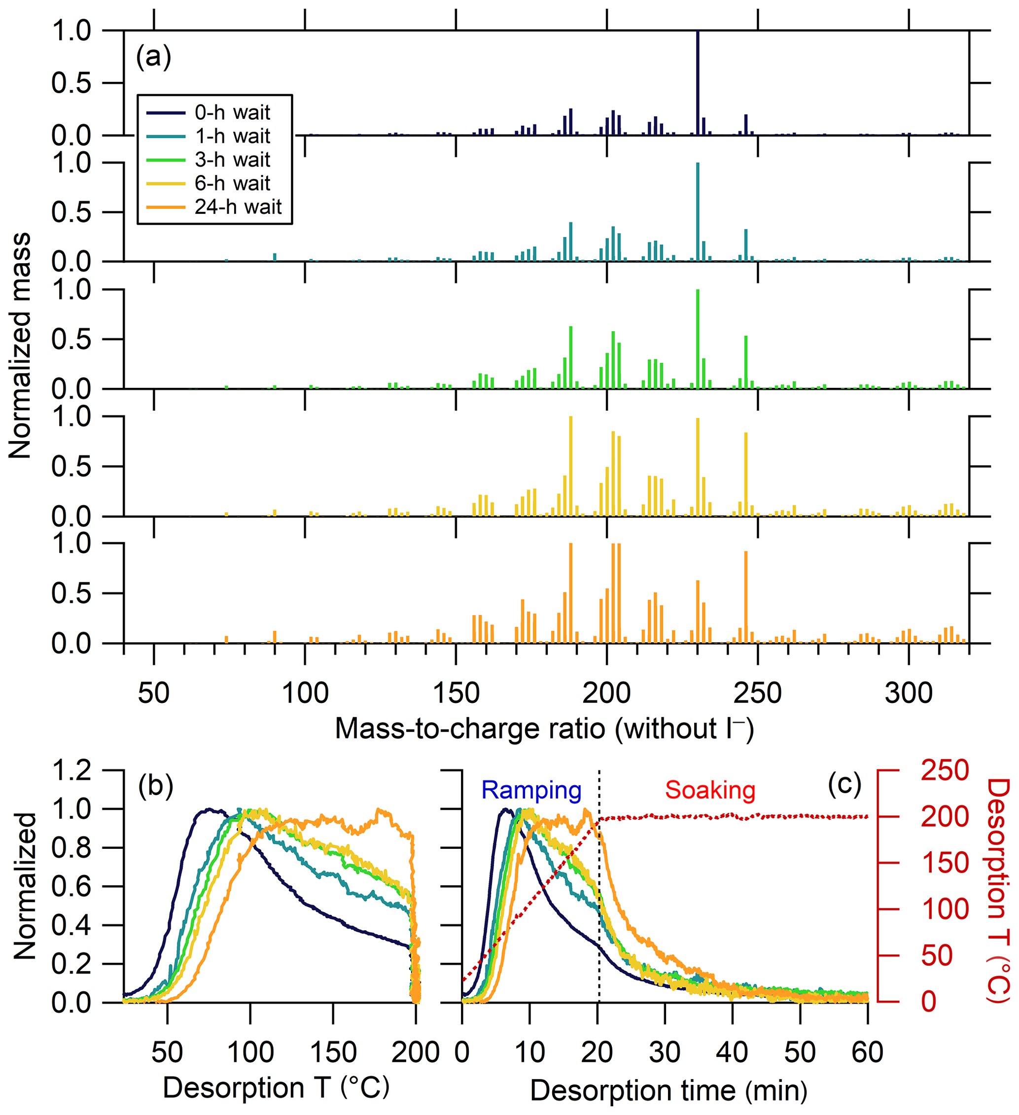
Figure 11(a) Normalized mass spectra of α-pinene + O3 SOA measured after different extents of isothermal evaporation at room temperature. The mass excludes iodine. The normalized thermograms of bulk SOA versus (b) temperature and (c) time, with the desorption temperature shown as a red dashed line. The vertical black dashed line in (c) delineates between ramping and soaking. The mass spectrum or thermogram colors indicate the isothermal evaporation time (see legend), with darker colors indicating shorter times.
There are 12 clusters determined from the no-wait experiment exhibiting a wide variety of shapes (Fig. 12a), with the parameters used for data preprocessing and clustering reported in Table 3 and shown in Fig. S5. Focusing first on the no-wait experiment, the cluster thermogram shapes include those having clear peaks at relatively low temperatures (∼60 ∘C) and with a sharp rise and fall (e.g., Clst nos. 1–3), those having sharp peaks at relatively low temperatures but with a shallow downward slope (e.g., Clst no. 6), those with a broad peak at somewhat higher temperatures (∼100 ∘C) and long tails (e.g., Clst no. 7), and those having a wide peak at even higher temperatures ∼120 ∘C with a very broad rise and fall (e.g., Clst no. 10).
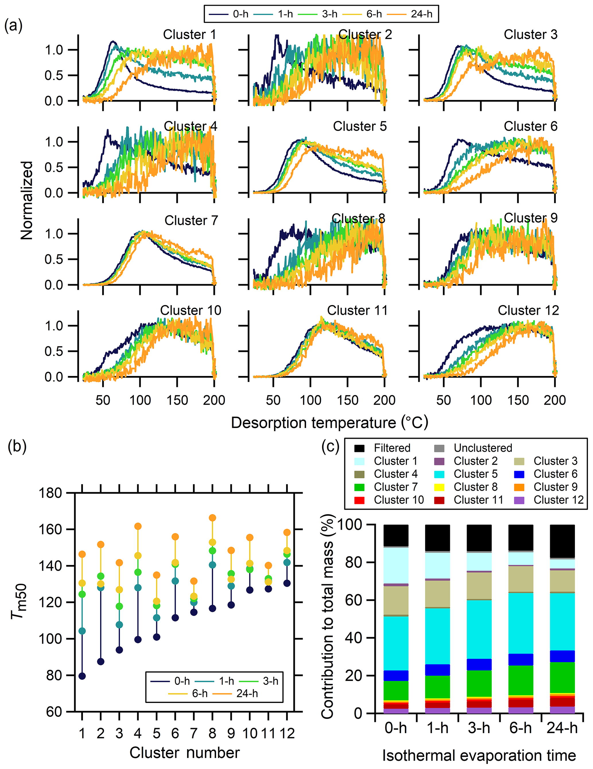
Figure 12Single-clustering results for α-pinene + O3 SOA for different isothermal evaporation times. (a) Comparison of the normalized, weighted average thermograms of the 12 clusters for the 0 h wait (navy), 1 h wait (blue), 3 h wait (green), 6 h wait (yellow), and 24 h wait (orange) experiments. Note that the absolute signals of all of the clusters decrease with evaporation but to varying extents (Fig. S6).
Changes to the shapes of the thermograms that occur upon isothermal evaporation differ between the clusters. Some of the clusters exhibit almost step changes from the no-wait to the longer time experiments (e.g., Clst nos. 2 and 6), while others exhibit more continuous changes (e.g., Clst nos. 3 and 5). However, in all cases the clusters shift to have peaks that occur at higher temperatures with generally broader thermograms. In other words, the Tm,50 of all the clusters increases as a function of evaporation time, but with larger increases observed for the clusters having initially lower Tm,50 (Fig. 12b). For some of the clusters with a clear peak below 100 ∘C, such as Clst nos. 1–6, the peaks broaden to become less obvious and shift to higher temperatures with longer isothermal evaporation. For clusters that originally have very wide peaks, such as Clst nos. 8–10 and 12, isothermal evaporation engenders a general shift in the thermograms towards higher temperatures. Different from the clusters described above, thermograms for two clusters, Clst no. 7 and Clst no. 11, exhibit only a minor shift of peak temperature and shapes. The thermograms of these two clusters share the common features of a moderate-width peak that reaches a maximum between 100 and 120 ∘C. The Tm,50 of these two clusters correspondingly exhibits small changes compared to other clusters.
Isothermal evaporation generally leads to a reduction of the monomeric character of clusters, leaving behind components that exhibit increased oligomeric content. Differences in how the individual cluster thermograms evolve with isothermal evaporation are therefore likely indicative of differing relative contributions of monomeric versus oligomeric components. For example, Clst no. 1 and Clst no. 10 have distinctly different shapes in the 0 h wait experiment but very similar shapes in the 24 h wait experiment. This indicates that ions in Clst no. 1 are not contributed from a single component, as might be inferred from the single-mode peak in the 0 h wait experiment. Instead, they are contributed by multiple components, though initially dominated by monomeric compounds, so the shift in peak temperature and broadness is substantial. On the other hand, ions in Clst no. 10 must also derive from multiple components, but with only a small fraction of monomeric compounds that evaporate in the 24 h. Consequently, the loss of low-temperature mass is apparent yet small. In contrast, ions in clusters such as Clst nos. 7 and 11 must be composed of only low-volatility components because they exhibit minimal changes in the thermogram shapes.
The extent of mass loss with isothermal evaporation differs between clusters. In general, clusters that exhibit larger changes in shape have greater total mass loss, although with variability (Fig. S6c). Consequently, the mass contributions of the clusters evolve with isothermal evaporation (Fig. 12b). The contribution of Clst no. 1 decreases significantly and most notably as wait time increases. The most prominent ion in the no-wait experiment, C10H14O6, is grouped in Clst no. 1. The continuous mass loss of Clst no. 1 indicates the rapid evaporation of its members. The mass contributions of the other clusters that exhibited similar changes in shape as Clst no. 1 (Clst nos. 3, 5, and 6) remain comparably constant, although with Clst no. 3 decreasing slightly. The relative abundances of the clusters for which the thermogram shapes changed negligibly (Clst nos. 7 and 11) increase continually, implying the slowest evaporation of the ions in these two clusters in the 24 h evaporation period.
For comparison, D'Ambro et al. (2018) reported changes in the shapes of the thermograms for the five most abundant individual ions from the no-wait to 24 h experiment, together carrying ∼15 % of the particle mass. They observed the individual ion thermograms generally all evolved in a manner similar to our Clst nos. 1, 3, and 5, shifting from narrower, more peaked profiles towards broader profiles with a shallower rise, less evident peak, and increased evaporation at higher temperatures. Here, with the clustering of data, we are able to track the change in the thermal behaviors of ions carrying ∼87 % of the initial mass. We are able to confirm that ∼70 % of the mass exhibits similar thermal behaviors and responses to isothermal evaporation as the top five ions. However, we are also able to identify another ∼17 % of the mass having initial thermograms not characterized by the top five ions, including 12 % of the mass (Clst nos. 7 and 11) that behaves distinctly differently upon evaporation at room temperature.
4.4.2 Multiple clustering
The number of clusters identified with the multiple-clustering method, using experiment-specific optimal ε values (Table 3 and Fig. S7), decreases with isothermal evaporation time from 13 (no-wait) to 12 (1 h) to 11 (3 h) and then to 9 (6 and 24 h) (Fig. 13b–f). The noise levels of the thermograms increase with evaporation time due to decreasing absolute particle mass. Nonetheless, the typical shapes of the cluster-specific thermograms clearly evolve with increasing isothermal evaporation. For short isothermal evaporation times, many cluster-specific thermogram profiles are relatively narrow, peaking at lower temperatures (70–120 ∘C) and with rapid rises and evident downslopes. For longer isothermal evaporation times, the cluster-specific profiles instead have broad peaks with slow rises and most of the mass desorbing at higher temperatures.

Figure 13Multiple-clustering results for α-pinene + O3 SOA as a function of isothermal evaporation time. (a) The contribution of each cluster to the total mass for each experiment, along with the contributions of filtered-out ions (black bar) and unclustered ions (gray bar). The number of clusters obtained generally decreases with isothermal evaporation time. (b–f) The unweighted average (gray) and mass-weighted average (black) thermograms, along with the thermograms of individual members of clusters for the (b) 0 h, (c) 1 h, (d) 3 h, (e) 6 h, and (f) 24 h wait experiments. The cluster colors are consistent between panels.
To aid further general interpretation, the cluster-specific thermograms with ∘C are grouped together as higher-volatility clusters. The number of higher-volatility clusters decreases with isothermal evaporation, from 10 for the no-wait experiment, to five in the 1 h experiment, two in the 3 and 6 h experiment, to none in the 24 h experiment (Fig. 14). The mass contributions of the higher-volatility clusters decrease from 81.9 % to 60.4 %, 17.2 %, 9.4 %, and to 0.0 % with increasing isothermal evaporation time. This overall behavior is consistent with results from the single-clustering method and indicates the compounds with a wide range of volatilities make up much of the mass in the initial particles, while the SOA after isothermal evaporation is composed of compounds having lower volatilities.
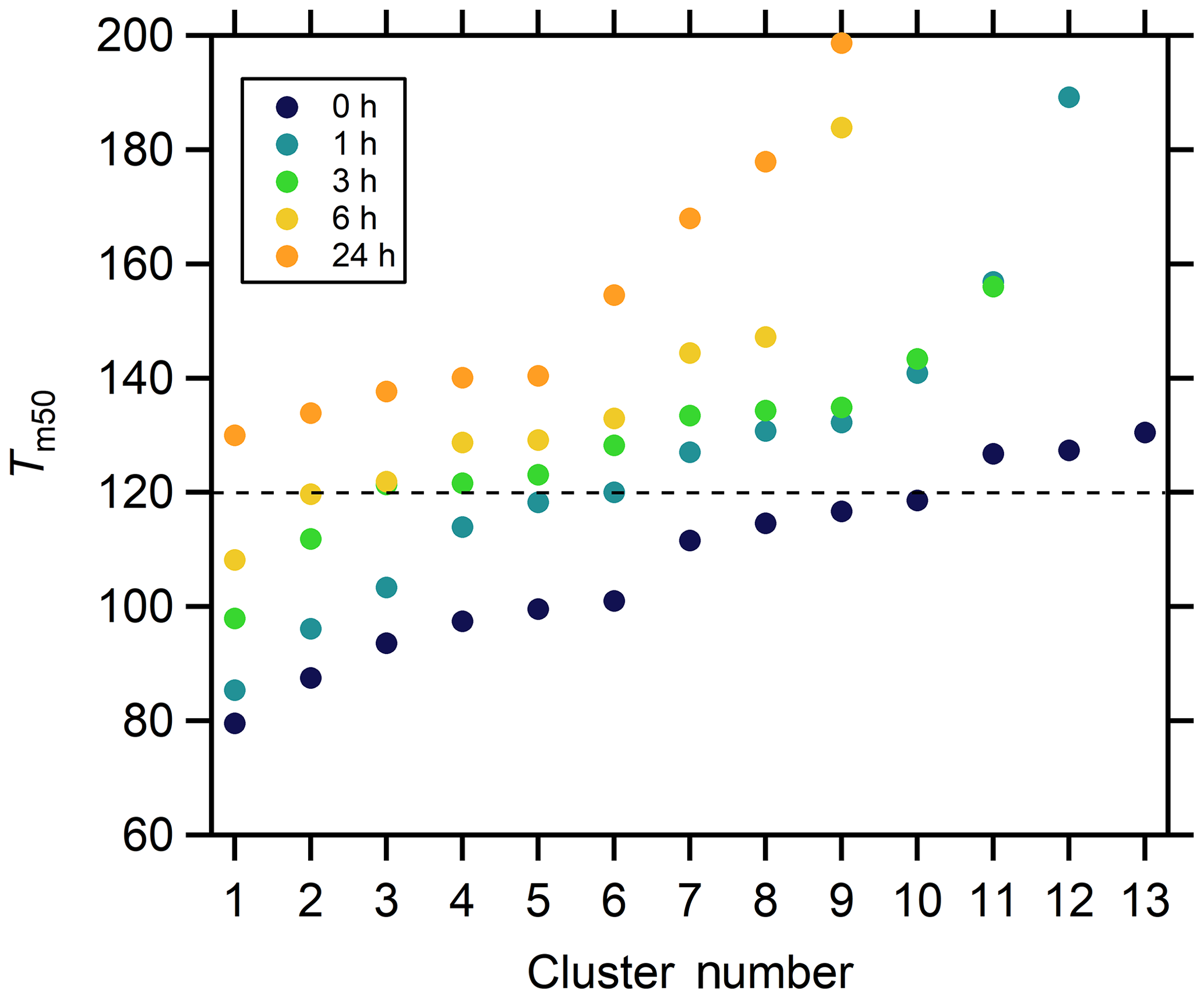
Figure 14The Tm,50 values of the cluster-specific thermograms from multiple clustering for the five isothermal evaporation experiments.
After isothermal evaporation, some cluster-specific thermograms have signals that increase continuously during the ramping period, for example Clst nos. 11 and 12 in the 1 h experiment; such clusters were not observed in the no-wait experiment. The relative abundance of these very low-volatility clusters increases with isothermal evaporation, from 1.7 % in the 1 h experiment (Clst nos. 11 and 12) to 13.4 % in the 24 h experiment (Clst nos. 7 and 9). The absence of these clusters for the no-wait experiment suggests that they are formed over time through condensed-phase reactions. Their increasing contribution over time may reflect both the evaporation of higher-volatility components and continued formation. Clusters having thermograms with very broad peaks, such as Clst nos. 11 and 13 in the 0 h experiment, are also observed in all the other experiments, with an increasing contribution to the total mass.
The multiple-clustering method reveals the disappearance of certain types of thermograms (e.g., the no-wait Clst no. 3) and the emergence of other types of thermograms (e.g., the 1 h Clst no. 11) as evaporation time increases. This complements the single-clustering method, which illustrates gradual changes in the shapes of cluster-specific thermograms, by allowing for the identification of completely new thermogram shapes and divergent behavior between ions within initial clusters. The multiple-clustering method also confirms the decrease in the diversity of the desorption profiles, as suggested by the single-clustering method. The two methods complement each other and together provide a detailed look into (i) how the desorption profiles of sets of ions evolve with isothermal evaporation and (ii) how the fraction of different types of thermograms changes with evaporation time.
We developed a new clustering algorithm, the noise-sorted scanning clustering (NSSC) algorithm, for application to FIGAERO-CIMS datasets. The NSSC algorithm provides a robust method for clustering FIGAERO-CIMS thermograms having distinct thermal desorption profiles and determining the mass contribution of each cluster. Each of the ions contributing to a cluster results from one or more molecules sharing similar thermochemical properties. These molecules either evaporate directly or decompose and then evaporate. Compared to other existing clustering algorithms, NSSC is strictly similarity-based, reproducible, and takes into consideration differences in noise levels between individual ions. The application of NSSC has the potential to make FIGAERO data more accessible to the atmospheric chemistry community.
For the four different SOA systems we examined, more than 80 % of the total mass is clustered, with the number of clusters ranging from 9 to 13. The shapes of the cluster-specific average thermograms exhibit substantial variation for a given system. Some have relatively sharp peaks, others broad peaks with slowly decreasing signal as heating continues, and others still having signals that continually increase up to very high temperatures or long desorption times. The mass contribution of a cluster varies from 0.2 % to 44.3 %. A few (two to three) clusters usually contain more than 50 % of the total mass in all the chemical systems examined. Comparison of the cluster-specific thermogram shapes between different SOA systems allows for a qualitative assessment of the similarity or uniqueness.
We also demonstrated the potential of the NSSC for guiding the interpretation of sets of experiments in which one experimental condition varies (e.g., NO concentration and evaporation time). For such experiments, two complementary methods are suggested: (i) the single-clustering method, whereby one experiment is used to determine the ions belonging to individual clusters and then clusters comprising the same ions are calculated for the other experiments, and (ii) the multiple-clustering method, whereby each experiment is clustered independently and then compared. The first approach helps establish how the properties of individual clusters evolve as a set, while the second approach helps identify changes in the diversity of cluster-specific thermogram shapes, properties, and mass contributions. The two approaches complement each other and provide guidance for future efforts to cluster ambient observations having long time series.
This paper focuses only on the description of the clustering algorithm and its potential as a tool to characterize the thermal properties of organic aerosol in further detail. The application of NSSC can be potentially expanded to any other composition-resolved datasets, such as diurnal changes in different compounds measured in ambient air, temporal changes in different generations of species in a smog chamber, and composition-dependent size distributions. All of the above datasets share a common property that the noise of the curve and/or spectrum is related to the composition. Therefore, NSSC would facilitate the analysis by taking noise into consideration. Interpretation of the cluster-specific thermograms using frameworks such as that of Schobesberger et al. (2018) will allow for a more comprehensive understanding of the thermochemical properties of the organic aerosol, which is the subject of future work. This will provide insights into the thermal behavior of organic aerosol and the relative contributions of thermally stable (e.g., monomer) versus thermally unstable (e.g., dimers or oligomers) compounds, the volatility distribution of the thermally stable compounds, and the T-dependent rate coefficients for oligomer dissociation and formation.
All data and the NSSC algorithm used in this publication are archived in the UC DASH data repository (https://doi.org/10.25338/B87S43; Cappa et al., 2019). The NSSC algorithm is also available at GitHub (https://github.com/chriscappa/NSSC, last access: 17 February 2020), with the version used for this publication available as Li and Cappa (2019, https://doi.org/10.5281/zenodo.3361797).
The supplement related to this article is available online at: https://doi.org/10.5194/acp-20-2489-2020-supplement.
ZL developed the NSSC algorithm. ELD'A, SS, CJG, FDLH, JL, JES, and ZL performed measurements. ELD'A and SS performed detailed data processing. ZL and CDC analyzed data and wrote the paper, with contributions from all coauthors.
The authors declare that they have no conflict of interest.
The SOAFFEE campaign was done at Pacific Northwest National Laboratory, supported by the U.S. Department of Energy (DOE) Office of Science, Office of Biological and Environmental Research, as part of the Atmospheric Systems Research (ASR) program. PNNL is operated for the DOE by the Battelle Memorial Institute under contract DE-AC05-76RL01830.
This research has been supported by the National Science Foundation (grant no. ATM-1151062) and the U.S. Department of Energy (grant nos. DE-SC0011791 and DE-SC0018221). Emma L. D'Ambro was supported by the National Science Foundation Graduate Research Fellowship (grant no. DGE-1256082), and Siegfried Schobesberger was supported by the Academy of Finland (grant nos. 272041 and 310682).
This paper was edited by Rob MacKenzie and reviewed by two anonymous referees.
Abdalmogith, S. S. and Harrison, R. M.: The use of trajectory cluster analysis to examine the long-range transport of secondary inorganic aerosol in the UK, Atmos. Environ., 39, 6686–6695, https://doi.org/10.1016/j.atmosenv.2005.07.059, 2005.
Beddows, D. C. S., Dall'Osto, M., and Harrison, R. M.: Cluster Analysis of Rural, Urban, and Curbside Atmospheric Particle Size Data, Environ. Sci. Technol., 43, 4694–4700, https://doi.org/10.1021/es803121t, 2009.
Cape, J. N., Methven, J., and Hudson, L. E.: The use of trajectory cluster analysis to interpret trace gas measurements at Mace Head, Ireland, Atmos. Environ., 34, 3651–3663, https://doi.org/10.1016/S1352-2310(00)00098-4, 2000.
Cappa, C. D., Li, Z., D'Ambro, E. L., Schobesberger, S., Shilling, J. E., Lopez-Hilfiker, F., Liu, J., Gaston, C. J., and Thornton, J. A.: Initial application of the noise-sorted scanning clustering algorithm to the analysis of composition-dependent organic aerosol thermal desorption measurements, UC Davis Dash, Dataset, https://doi.org/10.25338/B87S43, 2019.
D'Ambro, E. L., Lee, B. H., Liu, J., Shilling, J. E., Gaston, C. J., Lopez-Hilfiker, F. D., Schobesberger, S., Zaveri, R. A., Mohr, C., Lutz, A., Zhang, Z., Gold, A., Surratt, J. D., Rivera-Rios, J. C., Keutsch, F. N., and Thornton, J. A.: Molecular composition and volatility of isoprene photochemical oxidation secondary organic aerosol under low- and high-NOx conditions, Atmos. Chem. Phys., 17, 159–174, https://doi.org/10.5194/acp-17-159-2017, 2017.
D'Ambro, E. L., Schobesberger, S., Zaveri, R. A., Shilling, J. E., Lee, B. H., Lopez-Hilfiker, F. D., Mohr, C., and Thornton, J. A.: Isothermal Evaporation of alpha-Pinene Ozonolysis SOA: Volatility, Phase State, and Oligomeric Composition, ACS Earth Space Chem, 2, 1058–1067, https://doi.org/10.1021/acsearthspacechem.8b00084, 2018.
D'Ambro, E. L., Schobesberger, S., Gaston, C. J., Lopez-Hilfiker, F. D., Lee, B. H., Liu, J., Zelenyuk, A., Bell, D., Cappa, C. D., Helgestad, T., Li, Z., Guenther, A., Wang, J., Wise, M., Caylor, R., Surratt, J. D., Riedel, T., Hyttinen, N., Salo, V.-T., Hasan, G., Kurtén, T., Shilling, J. E., and Thornton, J. A.: Chamber-based insights into the factors controlling epoxydiol (IEPOX) secondary organic aerosol (SOA) yield, composition, and volatility, Atmos. Chem. Phys., 19, 11253–11265, https://doi.org/10.5194/acp-19-11253-2019, 2019.
Faxon, C., Hammes, J., Le Breton, M., Pathak, R. K., and Hallquist, M.: Characterization of organic nitrate constituents of secondary organic aerosol (SOA) from nitrate-radical-initiated oxidation of limonene using high-resolution chemical ionization mass spectrometry, Atmos. Chem. Phys., 18, 5467–5481, https://doi.org/10.5194/acp-18-5467-2018, 2018.
Gaston, C. J., Quinn, P. K., Bates, T. S., Gilman, J. B., Bon, D. M., Kuster, W. C., and Prather, K. A.: The impact of shipping, agricultural, and urban emissions on single particle chemistry observed aboard the R/V Atlantis during CalNex, J. Geophys. Res.-Atmos., 118, 5003–5017, https://doi.org/10.1002/jgrd.50427, 2013.
Gaston, C. J., Lopez-Hilfiker, F. D., Whybrew, L. E., Hadley, O., McNair, F., Gao, H. L., Jaffe, D. A., and Thornton, J. A.: Online molecular characterization of fine particulate matter in Port Angeles, WA: Evidence for a major impact from residential wood smoke, Atmos. Environ., 138, 99–107, https://doi.org/10.1016/j.atmosenv.2016.05.013, 2016.
Giorio, C., Tapparo, A., Dall'Osto, M., Harrison, R. M., Beddows, D. C. S., Di Marco, C., and Nemitz, E.: Comparison of three techniques for analysis of data from an Aerosol Time-of-Flight Mass Spectrometer, Atmos. Environ., 61, 316–326, https://doi.org/10.1016/j.atmosenv.2012.07.054, 2012.
Goldstein, A. H. and Galbally, I. E.: Known and unexplored organic constituents in the earth's atmosphere, Environ. Sci. Technol., 41, 1514–1521, https://doi.org/10.1021/es072476p, 2007.
Gonzalez, T. F.: Clustering to Minimize the Maximum Intercluster Distance, Theor. Comput. Sci., 38, 293–306, https://doi.org/10.1016/0304-3975(85)90224-5, 1985.
Hamilton, J. F., Webb, P. J., Lewis, A. C., Hopkins, J. R., Smith, S., and Davy, P.: Partially oxidised organic components in urban aerosol using GCXGC-TOF/MS, Atmos. Chem. Phys., 4, 1279–1290, https://doi.org/10.5194/acp-4-1279-2004, 2004.
Huang, W., Saathoff, H., Pajunoja, A., Shen, X., Naumann, K.-H., Wagner, R., Virtanen, A., Leisner, T., and Mohr, C.: α-Pinene secondary organic aerosol at low temperature: chemical composition and implications for particle viscosity, Atmos. Chem. Phys., 18, 2883–2898, https://doi.org/10.5194/acp-18-2883-2018, 2018.
Isaacman-VanWertz, G., Massoli, P., O'Brien, R. E., Nowak, J. B., Canagaratna, M. R., Jayne, J. T., Worsnop, D. R., Su, L., Knopf, D. A., Misztal, P. K., Arata, C., Goldstein, A. H., and Kroll, J. H.: Using advanced mass spectrometry techniques to fully characterize atmospheric organic carbon: current capabilities and remaining gaps, Faraday Discuss., 200, 579–598, https://doi.org/10.1039/c7fd00021a, 2017.
Joo, T., Rivera-Rios, J. C., Takeuchi, M., Alvarado, M. J., and Ng, N. L.: Secondary Organic Aerosol Formation from Reaction of 3-Methylfuran with Nitrate Radicals, Acs Earth Space Chem., 3, 6, https://doi.org/10.1021/acsearthspacechem.9b00068, 2019.
Kirchner, U., Vogt, R., Natzeck, C., and Goschnick, J.: Single particle MS, SNMS, SIMS, XPS, and FTIR spectroscopic analysis of soot particles during the AIDA campaign, J. Aerosol Sci., 34, 1323–1346, https://doi.org/10.1016/S0021-8502(03)00362-8, 2003.
Le Breton, M., Psichoudaki, M., Hallquist, M., Watne, A. K., Lutz, A., and Hallquist, A. M.: Application of a FIGAERO ToF CIMS for on-line characterization of real-world fresh and aged particle emissions from buses, Aerosol Sci. Tech., 53, 244–259, https://doi.org/10.1080/02786826.2019.1566592, 2019.
Lee, A. K. Y., Willis, M. D., Healy, R. M., Onasch, T. B., and Abbatt, J. P. D.: Mixing state of carbonaceous aerosol in an urban environment: single particle characterization using the soot particle aerosol mass spectrometer (SP-AMS), Atmos. Chem. Phys., 15, 1823–1841, https://doi.org/10.5194/acp-15-1823-2015, 2015.
Lee, B. H., Lopez-Hilfiker, F. D., Mohr, C., Kurten, T., Worsnop, D. R., and Thornton, J. A.: An Iodide-Adduct High-Resolution Time-of-Flight Chemical-Ionization Mass Spectrometer: Application to Atmospheric Inorganic and Organic Compounds, Environ. Sci. Technol., 48, 6309–6317, https://doi.org/10.1021/es500362a, 2014.
Lee, B. H., Mohr, C., Lopez-Hilfiker, F. D., Lutz, A., Hallquist, M., Lee, L., Romer, P., Cohen, R. C., Iyer, S., Kurten, T., Hu, W. W., Day, D. A., Campuzano-Jost, P., Jimenez, J. L., Xu, L., Ng, N. L., Guo, H. Y., Weber, R. J., Wild, R. J., Brown, S. S., Koss, A., de Gouw, J., Olson, K., Goldstein, A. H., Seco, R., Kim, S., McAvey, K., Shepson, P. B., Starn, T., Baumann, K., Edgerton, E. S., Liu, J. M., Shilling, J. E., Miller, D. O., Brune, W., Schobesberger, S., D'Ambro, E. L., and Thornton, J. A.: Highly functionalized organic nitrates in the southeast United States: Contribution to secondary organic aerosol and reactive nitrogen budgets, P. Natl. Acad. Sci. USA, 113, 1516–1521, https://doi.org/10.1073/pnas.1508108113, 2016.
Lee, B. H., Lopez-Hilfiker, F. D., D'Ambro, E. L., Zhou, P., Boy, M., Petäjä, T., Hao, L., Virtanen, A., and Thornton, J. A.: Semi-volatile and highly oxygenated gaseous and particulate organic compounds observed above a boreal forest canopy, Atmos. Chem. Phys., 18, 11547–11562, https://doi.org/10.5194/acp-18-11547-2018, 2018.
Li, Z. and Cappa, C. D.: Noise Sorted Scanning Clustering Algorithm (Version v1.0.3), Zenodo, https://doi.org/10.5281/zenodo.3361797, 2019
Liu, J. M., D'Ambro, E. L., Lee, B. H., Lopez-Hilfiker, F. D., Zaveri, R. A., Rivera-Rios, J. C., Keutsch, F. N., Iyer, S., Kurten, T., Zhang, Z. F., Gold, A., Surratt, J. D., Shilling, J. E., and Thornton, J. A.: Efficient Isoprene Secondary Organic Aerosol Formation from a Non-IEPDX Pathway, Environ. Sci. Technol., 50, 9872–9880, https://doi.org/10.1021/acs.est.6b01872, 2016.
Liu, S., Shilling, J. E., Song, C., Hiranuma, N., Zaveri, R. A., and Russell, L. M.: Hydrolysis of Organonitrate Functional Groups in Aerosol Particles, Aerosol Sci. Tech., 46, 1359–1369, https://doi.org/10.1080/02786826.2012.716175, 2012.
Liu, S., Russell, L. M., Sueper, D. T., and Onasch, T. B.: Organic particle types by single-particle measurements using a time-of-flight aerosol mass spectrometer coupled with a light scattering module, Atmos. Meas. Tech., 6, 187–197, https://doi.org/10.5194/amt-6-187-2013, 2013.
Lopez-Hilfiker, F. D., Mohr, C., Ehn, M., Rubach, F., Kleist, E., Wildt, J., Mentel, Th. F., Lutz, A., Hallquist, M., Worsnop, D., and Thornton, J. A.: A novel method for online analysis of gas and particle composition: description and evaluation of a Filter Inlet for Gases and AEROsols (FIGAERO), Atmos. Meas. Tech., 7, 983–1001, https://doi.org/10.5194/amt-7-983-2014, 2014.
Lopez-Hilfiker, F. D., Mohr, C., Ehn, M., Rubach, F., Kleist, E., Wildt, J., Mentel, Th. F., Carrasquillo, A. J., Daumit, K. E., Hunter, J. F., Kroll, J. H., Worsnop, D. R., and Thornton, J. A.: Phase partitioning and volatility of secondary organic aerosol components formed from α-pinene ozonolysis and OH oxidation: the importance of accretion products and other low volatility compounds, Atmos. Chem. Phys., 15, 7765–7776, https://doi.org/10.5194/acp-15-7765-2015, 2015.
Lopez-Hilfiker, F. D., Mohr, C., D'Ambro, E. L., Lutz, A., Riedel, T. P., Gaston, C. J., Iyer, S., Zhang, Z., Gold, A., Surratt, J. D., Lee, B. H., Kurten, T., Hu, W. W., Jimenez, J., Hallquist, M., and Thornton, J. A.: Molecular Composition and Volatility of Organic Aerosol in the Southeastern U.S.: Implications for IEPOX Derived SOA, Environ. Sci. Technol., 50, 2200–2209, https://doi.org/10.1021/acs.est.5b04769, 2016.
Mohr, C., Lopez-Hilfiker, F. D., Yli-Juuti, T., Heitto, A., Lutz, A., Hallquist, M., D'Ambro, E. L., Rissanen, M. P., Hao, L. Q., Schobesberger, S., Kulmala, M., Mauldin, R. L., Makkonen, U., Sipila, M., Petaja, T., and Thornton, J. A.: Ambient observations of dimers from terpene oxidation in the gas phase: Implications for new particle formation and growth, Geophys. Res. Lett., 44, 2958–2966, https://doi.org/10.1002/2017gl072718, 2017.
Murphy, D. M., Middlebrook, A. M., and Warshawsky, M.: Cluster analysis of data from the Particle Analysis by Laser Mass Spectrometry (PALMS) instrument, Aerosol Sci. Tech., 37, 382–391, https://doi.org/10.1080/02786820300971, 2003.
Pinero-Garcia, F., Ferro-Garcia, M. A., Chham, E., Cobos-Diaz, M., and Gonzalez-Rodelas, P.: A cluster analysis of back trajectories to study the behaviour of radioactive aerosols in the south-east of Spain, J. Environ. Radioactiv., 147, 142–152, https://doi.org/10.1016/j.jenvrad.2015.05.029, 2015.
Praske, E., Otkjaer, R. V., Crounse, J. D., Hethcox, J. C., Stoltz, B. M., Kjaergaard, H. G., and Wennberg, P. O.: Atmospheric autoxidation is increasingly important in urban and suburban North America, P. Natl. Acad. Sci. USA, 115, 64–69, https://doi.org/10.1073/pnas.1715540115, 2018.
Rebotier, T. P. and Prather, K. A.: Aerosol time-of-flight mass spectrometry data analysis: A benchmark of clustering algorithms, Anal. Chim. Acta, 585, 38–54, https://doi.org/10.1016/j.aca.2006.12.009, 2007.
Reitz, P., Zorn, S. R., Trimborn, S. H., and Trimborn, A. M.: A new, powerful technique to analyze single particle aerosol mass spectra using a combination of OPTICS and the fuzzy c-means algorithm, J. Aerosol Sci., 98, 1–14, https://doi.org/10.1016/j.jaerosci.2016.04.003, 2016.
Roth, A., Schneider, J., Klimach, T., Mertes, S., van Pinxteren, D., Herrmann, H., and Borrmann, S.: Aerosol properties, source identification, and cloud processing in orographic clouds measured by single particle mass spectrometry on a central European mountain site during HCCT-2010, Atmos. Chem. Phys., 16, 505–524, https://doi.org/10.5194/acp-16-505-2016, 2016.
Schobesberger, S., D'Ambro, E. L., Lopez-Hilfiker, F. D., Mohr, C., and Thornton, J. A.: A model framework to retrieve thermodynamic and kinetic properties of organic aerosol from composition-resolved thermal desorption measurements, Atmos. Chem. Phys., 18, 14757–14785, https://doi.org/10.5194/acp-18-14757-2018, 2018.
Song, X. H., Hopke, P. K., Fergenson, D. P., and Prather, K. A.: Classification of single particles analyzed by ATOFMS using an artificial neural network, ART-2A, Anal. Chem., 71, 860–865, https://doi.org/10.1021/ac9809682, 1999.
Stolzenburg, D., Fischer, L., Vogel, A. L., Heinritzi, M., Schervish, M., Simon, M., Wagner, A. C., Dada, L., Ahonen, L. R., Amorim, A., Baccarini, A., Bauer, P. S., Baumgartner, B., Bergen, A., Bianchi, F., Breitenlechner, M., Brilke, S., Mazon, S. B., Chen, D. X., Dias, A., Draper, D. C., Duplissy, J., Haddad, I., Finkenzeller, H., Frege, C., Fuchs, C., Garmash, O., Gordon, H., He, X., Helm, J., Hofbauer, V., Hoyle, C. R., Kim, C., Kirkby, J., Kontkanen, J., Kuerten, A., Lampilahti, J., Lawler, M., Lehtipalo, K., Leiminger, M., Mai, H., Mathot, S., Mentler, B., Molteni, U., Nie, W., Nieminen, T., Nowak, J. B., Ojdanic, A., Onnela, A., Passananti, M., Petaja, T., Quelever, L. L. J., Rissanen, M. P., Sarnela, N., Schallhart, S., Tauber, C., Tome, A., Wagner, R., Wang, M., Weitz, L., Wimmer, D., Xiao, M., Yan, C., Ye, P., Zha, Q., Baltensperger, U., Curtius, J., Dommen, J., Flagan, R. C., Kulmala, M., Smith, J. N., Worsnop, D. R., Hansel, A., Donahue, N. M., and Winkler, P. M.: Rapid growth of organic aerosol nanoparticles over a wide tropospheric temperature range, P. Natl. Acad. Sci. USA, 115, 9122–9127, https://doi.org/10.1073/pnas.1807604115, 2018.
Takahama, S., Gilardoni, S., Russell, L. M., and Kilcoyne, A. L. D.: Classification of multiple types of organic carbon composition in atmospheric particles by scanning transmission X-ray microscopy analysis, Atmos. Environ., 41, 9435–9451, https://doi.org/10.1016/j.atmosenv.2007.08.051, 2007.
Wang, D. S. and Hildebrandt Ruiz, L.: Chlorine-initiated oxidation of n-alkanes under high-NOx conditions: insights into secondary organic aerosol composition and volatility using a FIGAERO–CIMS, Atmos. Chem. Phys., 18, 15535–15553, https://doi.org/10.5194/acp-18-15535-2018, 2018.
Wegner, T., Hussein, T., Hameri, K., Vesala, T., Kulmala, M., and Weber, S.: Properties of aerosol signature size distributions in the urban environment as derived by cluster analysis, Atmos. Environ., 61, 350–360, https://doi.org/10.1016/j.atmosenv.2012.07.048, 2012.
Zhao, W. X., Hopke, P. K., and Prather, K. A.: Comparison of two cluster analysis methods using single particle mass spectra, Atmos. Environ., 42, 881–892, https://doi.org/10.1016/j.atmosenv.2007.10.024, 2008.
Zhao, Y., Thornton, J. A., and Pye, H. O. T.: Quantitative constraints on autoxidation and dimer formation from direct probing of monoterpene-derived peroxy radical chemistry, P. Natl. Acad. Sci. USA, 115, 12142–12147, https://doi.org/10.1073/pnas.1812147115, 2018.
Zhou, L. M., Hopke, P. K., and Venkatachari, P.: Cluster analysis of single particle mass spectra measured at Flushing, NY, Anal. Chim. Acta, 555, 47–56, https://doi.org/10.1016/j.aca.2005.08.061, 2006.