First measurements of tides in the stratosphere and lower mesosphere by ground-based Doppler microwave wind radiometry

Atmospheric tides are important for vertical coupling in the atmosphere, from the stratosphere down to the troposphere and up to the thermosphere. They are planetary-scale gravity waves with well-known periods that are integer fractions of a day and can be observed in the temperature or wind fields in the atmosphere. Most lidar techniques and satellites measure atmospheric tides only in the temperature field and continuous measurements of the tides in the wind field of the stratosphere and lower mesosphere are rare, even though, with modern lidars, they would be feasible. In this study, we present measurements of the diurnal tide in the wind field in the stratosphere and lower mesosphere by ground-based microwave wind radiometry for two different campaigns in tropical and polar regions. Further, we compare our measurements to MERRA-2 reanalysis data. In the tri-monthly mean, we find a good correspondence in the amplitude and phase of the diurnal tide between measurements and reanalysis with the most important features of the diurnal tides represented in both data sets. When looking at shorter timescales, we find significant differences in the data sets. We make an attempt to examine these differences and discriminate between atmospheric variability and noise, and we present some hints for intermittent diurnal tides. We conclude that continuous ground-based observations of tides in the middle atmospheric wind field are feasible, and they deliver consistent results for the mean amplitude and phase of the diurnal tide in the tri-monthly mean. We further discuss the limitations in regards to short timescale observations of tides and the possibility to provide additional insight into middle atmospheric dynamics that is complementary to temperature observations and reanalysis data.

1 Introduction

Atmospheric tides are global-scale waves with well-known periods that are integer fractions of a day. They are the result of the periodic solar forcing of the temperature and wind fields and gravity as a restoring force. Just like other gravity waves, tidal waves can propagate up- or downwards, be reflected, and they ultimately deposit energy in the atmosphere when they break. This transport and deposition of energy can cause secondary waves and other disturbances, resulting in a vertical coupling between the horizontal layers of the atmosphere and leading to an exchange of energy and momentum between the forcing regions and the dissipation altitudes. Ultimately, tides in the stratosphere and mesosphere region can affect weather phenomena like, for example, the diurnal cycle of tropical rainfall (Woolnough et al., 2004; Sakazaki et al., 2018).

Due to the global nature of atmospheric tides, they have been studied over decades using models (Lindzen, 1971; Forbes and Wu, 2006; Wang et al., 2016) or global observations from satellites (Oberheide et al., 2009; Häusler et al., 2010; Pancheva and Mukhtarov, 2011). Considering the observational results, Oberheide et al. (2011) introduced a climatology-based model of atmospheric tides covering the most relevant diurnal and semi-diurnal tidal modes at altitudes between 80 and 400 km. While atmospheric tides are well understood and modelled (Hagan et al., 1999) on a global and seasonal scale, very little is known about tides on a local and sub-seasonal scale.

Tides in the temperature field have been extracted from satellite observations (Sakazaki et al., 2012; Forbes and Wu, 2006; McLandress et al., 1996; Oberheide et al., 2009) and have been compared to different reanalysis data sets by Sakazaki et al. (2018) from the stratosphere to the lower mesosphere. Satellites, however, often need several weeks to sample a full diurnal cycle for a specific location due to their orbit and therefore are not capable to resolve tidal variations at short timescales. The global coverage nevertheless also enables tidal studies on shorter timescales for instruments on these satellites under the assumption of a linear tide model (Ortland, 2017). Satellites with a sun-synchronous orbit, e.g. Aura MLS, overpass each location exclusively at two local times which are specific to the latitude of this location and thus their ability to resolve tides is limited.

Ground-based measurements of tides in the temperature field have been performed by day-light-capable lidars for the stratosphere by Kopp et al. (2015) and Baumgarten and Stober (2019), as well as from meteor radar temperatures (Stober et al., 2008) in the mesosphere and lower thermosphere (MLT) region. Meteor radar and medium-frequency (MF) radar observations are also suitable to obtain tides in the wind fields (Portnyagin et al., 1993, 2004; Merzlyakov et al., 2009; Jacobi, 2012; Wilhelm et al., 2019). Current lidar instruments are able to measure inertial gravity waves in the wind field on short timescales (Baumgarten et al., 2015) and are thus in theory also suited for the observation of atmospheric tides, but the necessity of clear sky conditions reduces the availability of long-term observations drastically, and no observations of atmospheric tides are available to date.

Rogers et al. (2016) derived the local solar time variation of wind at 95 km altitude by integrating a 5-year data set from different ozone radiometers. Rocket soundings of the tides in the wind and temperature fields have been performed by Lindzen and Chapman (1969) up to the upper stratosphere, but they have never been repeated again.

Note that no observations of tides in the wind field for the stratosphere and lower mesosphere have so far been performed.

This leaves reanalysis data with high temporal resolution, like ERA5 and MERRA-2, as the only source for the wind field in studies about atmospheric tides. These products typically depend on satellite measurements, and thus tides in the upper atmospheric region are poorly constrained. Recent findings by Sakazaki et al. (2018) suggest that for the temperature field, differences between the different reanalyses and measurements are systematic in amplitude (approx. 1 K or 50 % above 40 km for northern mid-latitudes, more in the tropics), and the spread between the reanalyses is quite large in the lower mesosphere (0.3 to 1 K at approx. 60 km for northern mid-latitudes).

Recently, the temporal variability of tides at the MLT, which act as lower forcing of the ionospheric and thermospheric systems, became more and more important (e.g. Liu, 2016). There are currently several global circulation models (GCMs) developed which are supposed to describe consistently the vertical coupling between the middle atmosphere and the ionospheric thermospheric system (Pancheva et al., 2012; Yiğit et al., 2016; Liu et al., 2018). In particular, the short-term variability of the tidal forcing is essential for driving the more complex neutral-ionospheric coupling in the upper atmosphere. McCormack et al. (2017) presented a comparison between a meteorological reanalysis from the Navy Global Environmental Model – High Altitude (NAVGEM-HA) and several world-wide distributed meteor radars indicating substantial day-to-day variability of the winds and tides. Recently, Baumgarten and Stober (2019) presented a 10 d continuous lidar observation conducted with the Kühlungsborn Rayleigh–Mie–Raman lidar and estimated the tidal variability using an adaptive spectral filter technique (Stober et al., 2017). They complemented these observations with reanalysis data to investigate the phase relations of temperature and wind tides. However, lidar observations require cloud-free conditions, which usually limits the continuity of such time series.

In this study, we use measurements from the ground-based microwave Doppler wind radiometer WIRA-C (WInd RAdiometer for Campaigns), which can provide continuous measurements of the wind fields in the stratosphere and lower mesosphere (Hagen et al., 2018). The biggest advantage of the radiometers compared to many other ground-based remote-sensing instruments is their ability to measure continuously and independent of daylight and light clouds. Further, their compact design makes it rather easy to deploy these instruments at remote locations and enables their autonomous operation. Rüfenacht et al. (2018) performed an initial validation of the technique with other ground-based instruments, e.g. the ALOMAR (Arctic Lidar Observatory for Middle Atmosphere Research) lidar and the Andenes meteor radar. Particularly when compared to lidar, radiometers often have much coarser vertical and temporal resolutions. Rüfenacht et al. (2016) examined the spectrum of the wind oscillations for radiometric measurements and model data for periods down to 5 d, which is the lower limit of such an analysis due the low temporal resolution of wind radiometry. In this study, we present a method to investigate sub-day periods of oscillations with microwave wind radiometry by applying a different preprocessing to the measured spectra.

Specifically, we present a method to infer diurnal tides and their variability in the wind field in the stratosphere and lower mesosphere. After a short introduction to the measurement principle and analysis methods, we present the measurements from two WIRA-C campaigns, one was conducted on Réunion island at tropical latitudes and the other one on Andøya island at polar latitudes. We show that our instrument is able to capture the mean diurnal wind tide over the course of a 3-month period, and we compare our measurements to the meteorological reanalysis MERRA-2 (GMAO, 2015) with respect to the amplitude and phase behaviour. We do this comparison for tri-monthly means as well on shorter timescales (days or weeks) to reveal some differences between the observations and the reanalysis.

The article is structured as follows. In Sect. 2 we present a summary of the instrument and the campaigns. The data analysis and retrievals are described in Sect. 3. Our results are presented in Sect. 4, and our conclusions are given in Sect. 5.

2 The WIRA-C instrument and campaigns

2.1 Instrument

The WIRA-C instrument is a Doppler microwave wind radiometer. As described in detail by Hagen et al. (2018), it measures the 142 GHz ozone rotational emission line with a high spectral resolution of 12.5 kHz. Because the ozone molecules are moving with the mean air flow, the Doppler shift introduced to the emission line is directly proportional to the line-of-sight wind speed. In order to be sensitive to the zonal and meridional component of the horizontal wind speed, we observe the emission line for all cardinal directions (north, east, south, west) at a low elevation angle of 22^∘. Further, the pressure-broadening effect allows for the retrieval of altitude-resolved wind profiles in an altitude range from 30 to 75 km on a 3 km vertical grid with 12 km vertical resolution.

WIRA-C has an un-cooled but temperature-stabilized receiver with a low receiver noise temperature due to a state-of-the-art low-noise amplifier that directly amplifies the observation frequency of 142 GHz. Despite the low noise, integration times of 12 to 24 h are typically applied in the standard retrievals. These long integration times are required to achieve a signal-to-noise ratio that is sufficient for a retrieval of wind speed.

WIRA-C operates autonomously and automatically and the measurements are independent of daylight and light clouds with interruptions only during rain or heavy snowfall. Additionally WIRA-C uses a tipping curve calibration scheme, and thus it only needs very minimal maintenance, most of which can be done remotely. As a result, the WIRA-C instrument is especially well suited for campaigns as well as long-term monitoring observations.

The forward model for the retrieval is supplied by the ARTS software package (Buehler et al., 2018). The inversion of the measured spectra is performed by an optimal estimation method (OEM) developed by Rodgers (2000). We use the OEM algorithm that has recently been implemented directly into the ARTS software.

Optimal estimation is a method where the ill-posed inversion problem is regularized by an a priori profile and a corresponding covariance matrix. It is well suited for the inversion of atmospheric measurements, because the mean background state is often known reasonably well. This applies to this study in particular, where the mean background wind speed is known from models and measurements to a reasonable extent, and the diurnal cycle can be understood as a perturbation of the background state that we can retrieve from the measurements.

Different quality control parameters can be derived for an optimal estimation of a profile. The measurement response, which is the most important to us, estimates the sensitivity of the retrieved quantity to actual changes in the observed system (as opposed to sensitivity to the a priori profile). Ideally, this measurement response is one, with 0.8 or 0.6 being acceptable numbers.

2.2 Campaigns

WIRA-C has been on two major campaigns so far. The first campaign started in August 2016 and took place in the Southern Hemisphere at the Maïdo observatory on Réunion island (France) (Baray et al., 2013), located in the Indian Ocean at 21^∘ S, 55^∘ E. The Maïdo observatory is located at an altitude of 2200 m a.s.l., which provides ideal conditions for radiometry. At this altitude there is less absorption due to tropospheric water vapour, which could be a problem in the tropics at lower altitudes. For tropical latitudes around $\pm \mathrm{30}{}^{\circ }$, the global scale wave model GSWM (Hagan et al., 1999) predicts a high amplitude of the diurnal tide compared to more polewards or more equatorial latitudes. The campaign ended in January 2018, and we refer to this as the tropical campaign.

For the second (and still ongoing) campaign, WIRA-C was moved to arctic latitudes in June 2018. The instrument is located at the ALOMAR observatory on Andøya (Norway) at 69^∘ N, 16^∘ E. We refer to this as the arctic campaign. The ALOMAR observatory is located on mount Ramnan, at 370 m a.s.l., and hosts many other remote-sensing instruments, e.g. the ALOMAR Rayleigh–Mie–Raman lidar, an Fe-lidar and several radars in the vicinity. The water vapour cycle at ALOMAR is dominated by the tropospheric weather pattern of the marine climate and variable within days rather than within a day.

3 Data processing

For the standard WIRA-C time series retrievals as used in previous studies, the spectra are integrated over continuous blocks of 12 or 24 h, resulting in a time series of wind speed with the same resolution (Hagen et al., 2018). Typically, for the tropical site, an integration over 12 h from sunrise to sunset is performed. However, for the retrieval of the daily cycle, we now aggregate the measurements of the same time of day over multiple days to perform a composite analysis. Typically, we use a window of 7 to 13 d and aggregate by time of day with a 2 to 4 h resolution. This gives a total integration time of around 20 h, centred around a central day. We refer to the different composites by (δD, δH), where δD indicates the number of days and δH the number of hours for the integration. The main composite used in this study is (13, 2), which gives a total integration time of 26 h.

After integration we run the wind retrieval for the WIRA-C instrument. For MERRA-2 reanalysis data, we apply the same aggregation directly on the model data to get the same temporal smoothing that we have to apply to our measurements. In addition, we also analyse the original reanalysis data.

A major difference to the retrieval described by Hagen et al. (2018) is that we use a non-zero wind a priori profile that corresponds to the mean wind background. This mitigates the effect of the diurnal variability of the troposphere on our measurements. If a zero-wind a priori is used, increased noise during daytime could lead to an overestimation of tidal amplitudes in the subsequent analysis, because the retrieved wind speed would be closer to zero (and thus possibly further away from the background) in the case of increased noise during daytime. In contrast, a mean-background a priori in combination with poor measurement response would lead to an underestimation of tidal amplitudes. This is especially important for locations with high diurnal variability (like our tropical site) or frequent rainfall (like our arctic site close to the sea). We extract the mean wind background from ECMWF operational data and average over the full 13 d centred around the (13, 2) composite, analogously to the other composites. Like this, our a priori wind profile does not include any tidal information at all. For the ozone a priori data, we aggregate WACCM data from Schanz et al. (2014), analogously to our measurements.

Once we have retrieved the wind profiles (or extracted them from the reanalysis data), we fit a simple tidal model to extract amplitude and phase information. The simple model for an arbitrary observable quantity y has the form of

$$\begin{array}{}\text{(1)}& {\displaystyle }y\left(t\right)& {\displaystyle }=c+\sum _{k=\mathrm{1}\mathrm{\dots }N}{A}_k\cos \left(t{\displaystyle \frac{\mathrm{2}\mathit{\pi }}{P_k}}-{\mathit{\varphi }}_k\right)\text{(2)}& {\displaystyle }& {\displaystyle }=c+\sum _{k=\mathrm{1}\mathrm{\dots }N}\left[a_k\cos \left(t{\displaystyle \frac{\mathrm{2}\mathit{\pi }}{P_k}}\right)+b_k\sin \left(t{\displaystyle \frac{\mathrm{2}\mathit{\pi }}{P_k}}\right)\right],\end{array}$$

where $P_k=\mathrm{24},\mathrm{12},\mathrm{8},\mathrm{\dots }$ h is the period of the diurnal, semi-diurnal and ter-diurnal tide. In this study we use N=1 and only consider the diurnal tide, but we write down the full basis in Eq. (2) to point out that the components for $k=\mathrm{1},\mathrm{2},\mathrm{3},\mathrm{\dots }$ are orthogonal and can thus be treated separately. We apply a least-squares optimization on Eq. (2) for the zonal and meridional wind components, and we assume the same weight for all wind measurements. Additionally, we estimate the uncertainty of the fit from the error covariance matrix of the adjusted parameters.

Equation (1) defines the phase ϕ_k as the time of day when the corresponding wind component has its maximum. Note that we present phases in units of mean solar time, so, for example, a phase of 10 h means that the maximum occurs 2 h before noon of the mean solar day. The amplitude A₁ and phase ϕ₁ of the diurnal tide are finally given by

$$\begin{array}{}\text{(3)}& {\displaystyle }{A}_{\mathrm{1}}& {\displaystyle }=\sqrt{a_{\mathrm{1}}^{\mathrm{2}}+b_{\mathrm{1}}^{\mathrm{2}}},\text{(4)}& {\displaystyle }{\mathit{\varphi }}_{\mathrm{1}}& {\displaystyle }=\text{acrtan2}\left(b_{\mathrm{1}},a_{\mathrm{1}}\right)\in (-\mathit{\pi },\mathit{\pi }].\end{array}$$

Since we average over multiple days prior to the retrieval, we do not apply a windowing function for the fitting of the tide as it is often suggested to compensate for the intermittency of waves. We assume that the retrieval of averaged spectra yields the average wind speed, so windowing and aggregation can be considered equivalent. This assumption might not hold true in the context of fast changes in the wind field, and we thus prefer periods of a stable wind background for our detailed analysis. We especially do not attempt to retrieve tidal parameters during strong planetary wave activity nor in the context of extreme events like sudden stratospheric warmings. Further, we consider non-tidal gravity waves to be filtered out by the vertical smoothing of the instrument of about 12 km.

Vertical smoothing (artificially or due to instrumental properties) decreases tidal amplitudes depending on the vertical wavelength of the observed tides. If the vertical wavelength is infinite (tidal phase is constant with altitude) the amplitude is not affected, whereas at typical vertical wavelengths of the diurnal tide of around 30 km, the smoothing can reduce the observed amplitude by up to 0.25. In this study, we do not apply any vertical smoothing to the reanalysis data.

To check for the significance and robustness of the diurnal tidal parameters, we compare the outcome for different composites. We run the same analysis for the (13, 2), (11, 2), (9, 3), (9, 2), (7, 4) and (7, 3) composites, which provide different samplings of the same observable. The similarities and differences among all the composites indicate how robust the parameters are and allow us to estimate the influence of noise from instrumental and atmospheric sources in a qualitative way.

We also compute the mean amplitude and phase over a larger time span (3 months) by averaging the wind field prior to fitting the tide model. We estimate the uncertainty of the amplitude and phase for the tri-monthly mean using a bootstrapping method that follows the moving block bootstrap (Lahiri, 2003, p.25ff). For a (δD, δH) composite time series, we sample a synthetic 3-month period (91 d) by choosing $\frac{\mathrm{91}}{\mathit{\delta }\mathrm{D}}$ composite days at random, and we estimate the diurnal tidal parameters of the mean diurnal cycle for each sample. The distribution of the parameters gives us an estimate of the uncertainty due to observational errors as well as due to phase variability during the period of observation.

4 Results

From both campaigns we select a 3-month period based on the following criteria. First we look for periods with stable background wind conditions. Due to the aggregation (maximum 13 d) for the wind retrieval, we prefer time intervals with no extreme meteorological events, e.g. sudden stratospheric warmings (SSWs), and a low planetary wave activity, because this might impact the retrieval of tidal amplitudes.

Further, we only considered time intervals with a good overall measurement response, which corresponds mainly to little precipitation. Another important aspect for the data analysis is the continuity of the observations (minimal instrumental downtime) to avoid issues in compiling the temporal averages.

Considering the above-mentioned criteria, we decided to focus on two campaign intervals from April to June 2017 at Maïdo and from September to November 2018 at Andenes (ALOMAR).

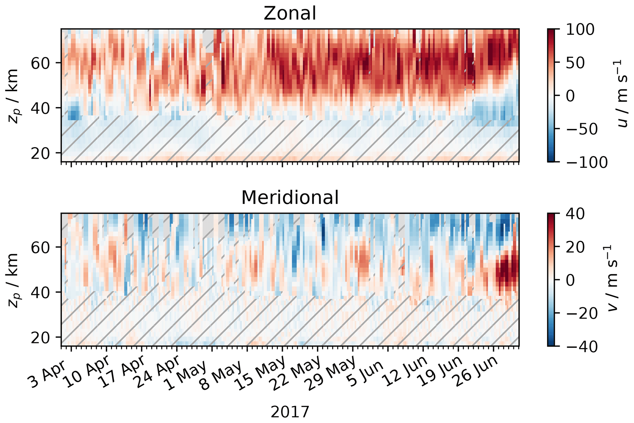
Figure 1 Background wind speed measured by WIRA-C complemented with MERRA-2 reanalysis data (hatching) for the tropical campaign. Note the different scales for the zonal and meridional components.

This gives us two time series for which we perform the previously described analysis: one for the tropical campaign and one for the arctic campaign. We use local mean solar time for all plots and phases in this study, which is simply a fixed offset depending on longitude. For the tropical campaign at 55.5^∘ E, this is an offset to Universal Time (UT) of 3.7 h. For the arctic campaign at 15.7^∘ E, the offset of local mean solar time to UT is 1 h.

4.1 Results for the tropical campaign

For the tropical campaign, we selected the period from April to June 2017. This period is at the beginning of austral winter, where the reanalysis as well as measurements shows a steady background of strong eastward winds with a small meridional component and relatively low planetary wave activity. Moreover, during this rather dry season, WIRA-C performed well and measured continuously with a good measurement response.

The meteorological background wind field for the selected period at the Maïdo observatory is shown in Fig. 1 as measured by WIRA-C, complemented with MERRA-2 reanalysis data for lower altitudes. The zonal and meridional winds indicate some variability at temporal scales of a few days. Characteristic of the zonal winds are westward winds below 40 km altitude and a strong zonal eastward stratospheric jet from 45 to 70 km altitude, which intensifies at the beginning of May. Meridional winds exhibit a steady change between southward and northward winds within a few days. Corresponding to the zonal wind enhancement, meridional winds become more southward at the beginning of May above a height of 60 km.

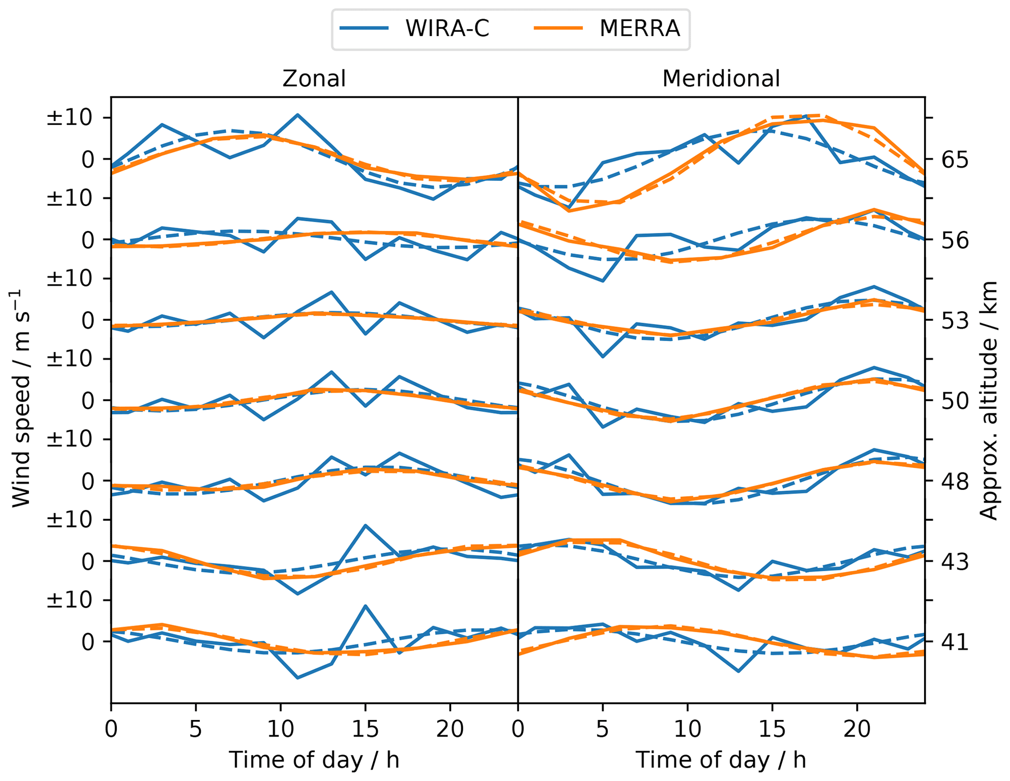
Figure 2 Mean daily cycle of zonal and meridional wind speeds at different altitudes for the 3 months during the tropical campaign from MERRA-2 and WIRA-C. Dashed lines indicate the best fit of the diurnal tide model.

The average diurnal cycle at different altitudes over the whole 3-month period is shown in Fig. 2 for WIRA-C measurements and the MERRA-2 reanalysis. In both data sets, the diurnal tide is readily visible. The reanalysis data seem not to contain any other modes than the diurnal tide, and the tide model from Eq. (2) fully fits the data. The measurements expose some more variability, especially at higher altitudes and during the afternoon hours. This is related to increased noise in the measurement in the afternoon hours, which is most prominent for the westward observation direction (and thus only seen in zonal wind retrievals) due to local weather patterns at the Maïdo observatory on Réunion island.

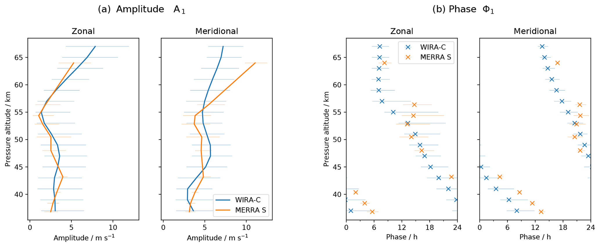
Figure 3 Amplitude and phase of mean daily cycle over 3 months from MERRA-2 reanalysis and WIRA-C measurements from the tropical campaign. Error bars indicate 95 % confidence limits. Phase is equivalent to solar time of maximum.

The agreement between MERRA-2 and the WIRA-C wind retrievals with respect to the mean behaviour can be assessed in Fig. 3. The left panel (Fig. 3a) shows the amplitude of the zonal and meridional mean diurnal cycle over the entire campaign period for WIRA-C and MERRA-2. Both data sets show a similar profile with relatively low amplitudes of less than 5 m s⁻¹ below 55 km and slightly higher amplitudes for the meridional component. Figure 3b shows the same for the vertical phase behaviour. The profiles of measurements and reanalysis are in agreement with respect to the amplitudes and phases up to an altitude of 55 km for the tropical location, where the reanalysis data lie within or are close to the limits of confidence of our measurements. The amplitude of the diurnal tide agrees for the measurement and reanalysis within or close to their limits of confidence. Above 55 km altitude, an increased discrepancy is evident for the meridional wind between MERRA-2 and the radiometer.

The phase of the mean daily cycle measured by WIRA-C as shown in Fig. 3b indicates a vertical wavelength of about 30 km. Approximately the same vertical wavelength is found in the reanalysis. Above 55 km altitude, the vertical wavelength of our measurements increases drastically, and the phase eventually becomes constant with altitude. Evidently, the tide seen by WIRA-C lags behind the tide represented in the reanalysis by 5 h at the lowermost altitude levels. Currently, we cannot explain this offset.

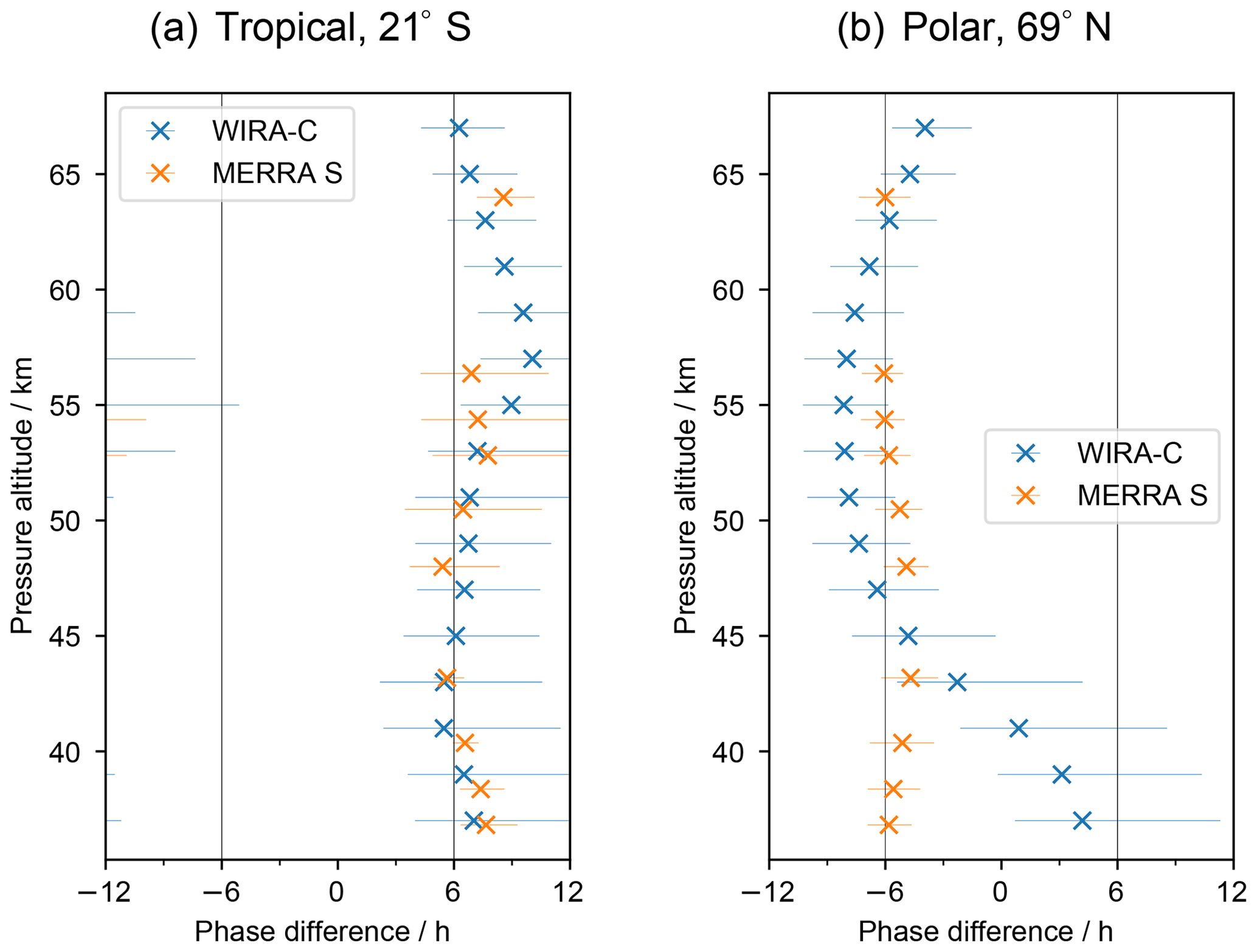
Figure 4 Phase difference between meridional and zonal diurnal wind tide ($\mathrm{\Delta }\mathit{\varphi }={\mathit{\varphi }}_{\mathrm{merid}.}-{\mathit{\varphi }}_{\mathrm{zonal}}$) for the tropical and arctic campaigns in WIRA-C measurements and the MERRA-2 reanalysis.

Figure 4b shows the phase difference between zonal and meridional diurnal tide. Measurements and reanalysis show a remarkable agreement and show that the meridional tide leads the zonal tide by approximately 6 h (90^∘ phase angle) as is expected for the Southern Hemisphere.

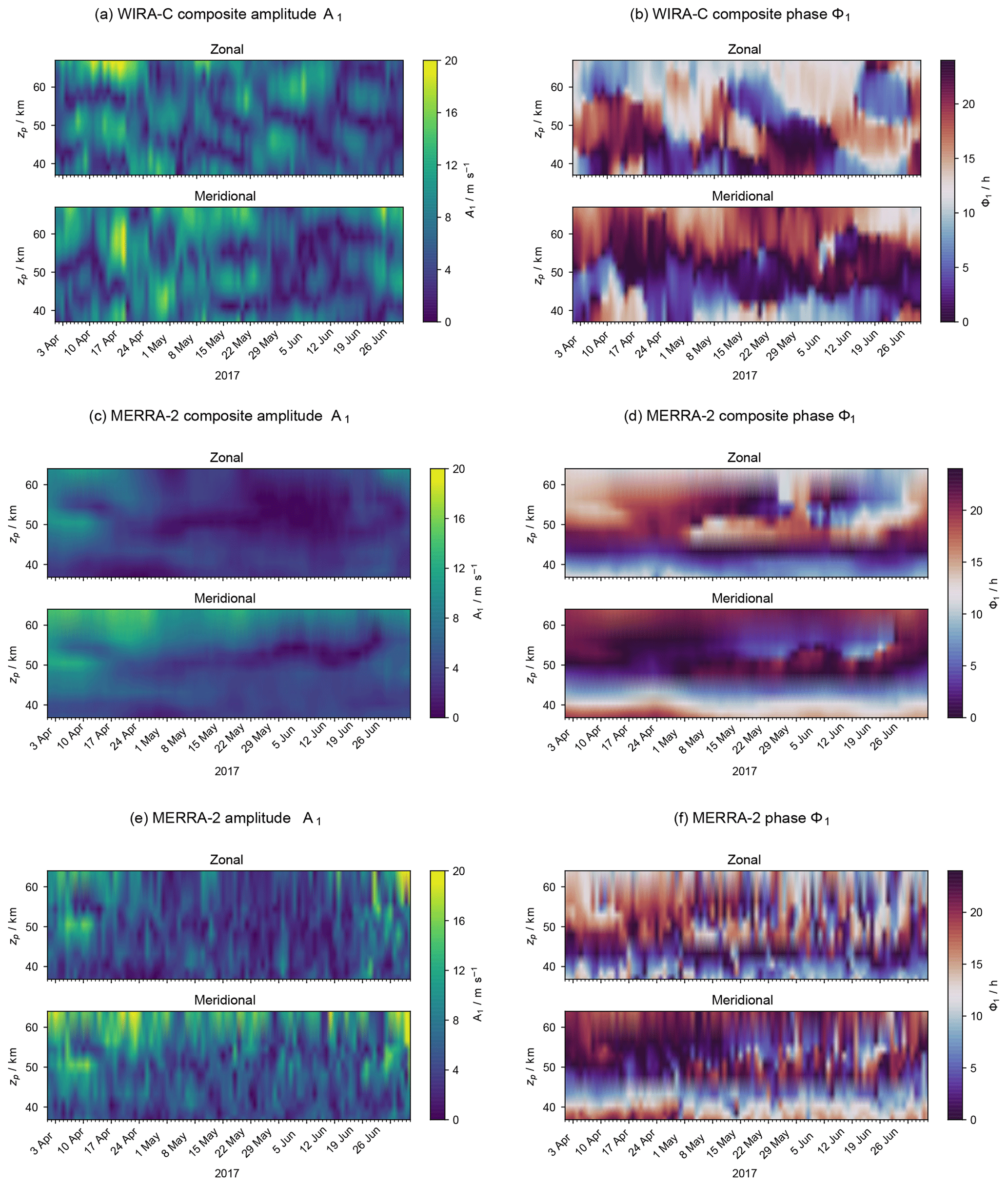
Figure 5 Amplitude and phase of the diurnal tide over 3 months from WIRA-C measurements (a, b), smoothed MERRA-2 reanalysis (c, d), and original MERRA-2 (e, f) during the tropical campaign at the Maïdo observatory.

Besides the tri-monthly mean, we show the diurnal tidal amplitude A₁ and phase ϕ₁ versus time for the whole period in Fig. 5. The upper two panels (Fig. 5a and b) show the WIRA-C retrievals. The central two panels (Fig. 5c and d) are obtained from the aggregated MERRA-2 reanalysis, whereas the bottom two panels (Fig. 5e and f) show the data for the original MERRA-2 reanalysis. These figures present the outcome for the (13, 2) composite only, and we provide five more composites in the Appendix in Figs. A1 and A2 for the tropical campaign. The WIRA-C diurnal tidal amplitudes reach a maximum at the beginning of the campaign of about 16 to 20 m s⁻¹ for both components. During the second phase of the campaign we observe smaller tidal amplitudes of approximately 4 to 12 m s⁻¹. The vertical structure that is obvious in Fig. 5a can also be seen in the tri-monthly mean (Fig. 3a) with a minimum at 55 km. Because we observe a similar oscillating pattern of tidal amplitude with altitude in measurements and reanalysis (Fig. 3a), we propose the mixing of different tidal waves with different vertical wavelengths or propagation directions as a possible source for this structure. The augmented magnitude of the structure in our measurements compared to reanalysis data might still be due to slight oscillations of the retrieval.

Further, our observations show a strong time dependence of the diurnal tidal amplitude and phase at the resolved temporal scales of 7 to 13 d. We observe the same morphology in the time series for all composites (Figs. A1 and A2), and we take this as a hint that the variability is not only due to noise. Nevertheless, there are some differences between the different composites, especially in the absolute values of the amplitudes that are most probably related to instrumental noise. The phase, on the other hand, is more robust, and the time series of the diurnal tidal phase has the same structure in all composites and exposes a pattern of the diurnal tidal phase modulated with a period of approximately a month.

Compared to the WIRA-C observations, the MERRA-2 reanalysis data show a constant amplitude and phase over time in the composite analysis (Fig. 5c and d). The original MERRA-2 data as shown in Fig. 5e and f are less constant over time, and phase and amplitude expose a high day-to-day variability. However, the mean behaviour seems to be in good agreement with the observations, and the general morphology of the diurnal tide in amplitude and phase seems to agree between measurements and reanalysis.

Figure 6 Time series of zonal and meridional diurnal tide amplitudes during the tropical campaign for measurements (WIRA-C), MERRA-2 reanalysis (MERRA) and reanalysis smoothed (MERRA s) at an altitude level of 53 km with corresponding errors of the model fit as shaded area.

Figure 6 shows a comparison of the time series between WIRA-C and the MERRA-2 reanalysis at an altitude of 55 km. The shaded area represents the uncertainties of the estimated diurnal tidal amplitudes taken from the covariance of the adjusted parameters. In addition to the MERRA-2 reanalysis that has been smoothed with our integration kernel, we show the tidal analysis of the original MERRA-2 data. This comparison indicates how the diurnal tidal amplitude decreases and increases again during the campaign in the measurements as well as in the reanalysis. MERRA-2 and our measurements show larger diurnal tidal amplitudes at the beginning of the tropical campaign in April, which then decrease in May and June.

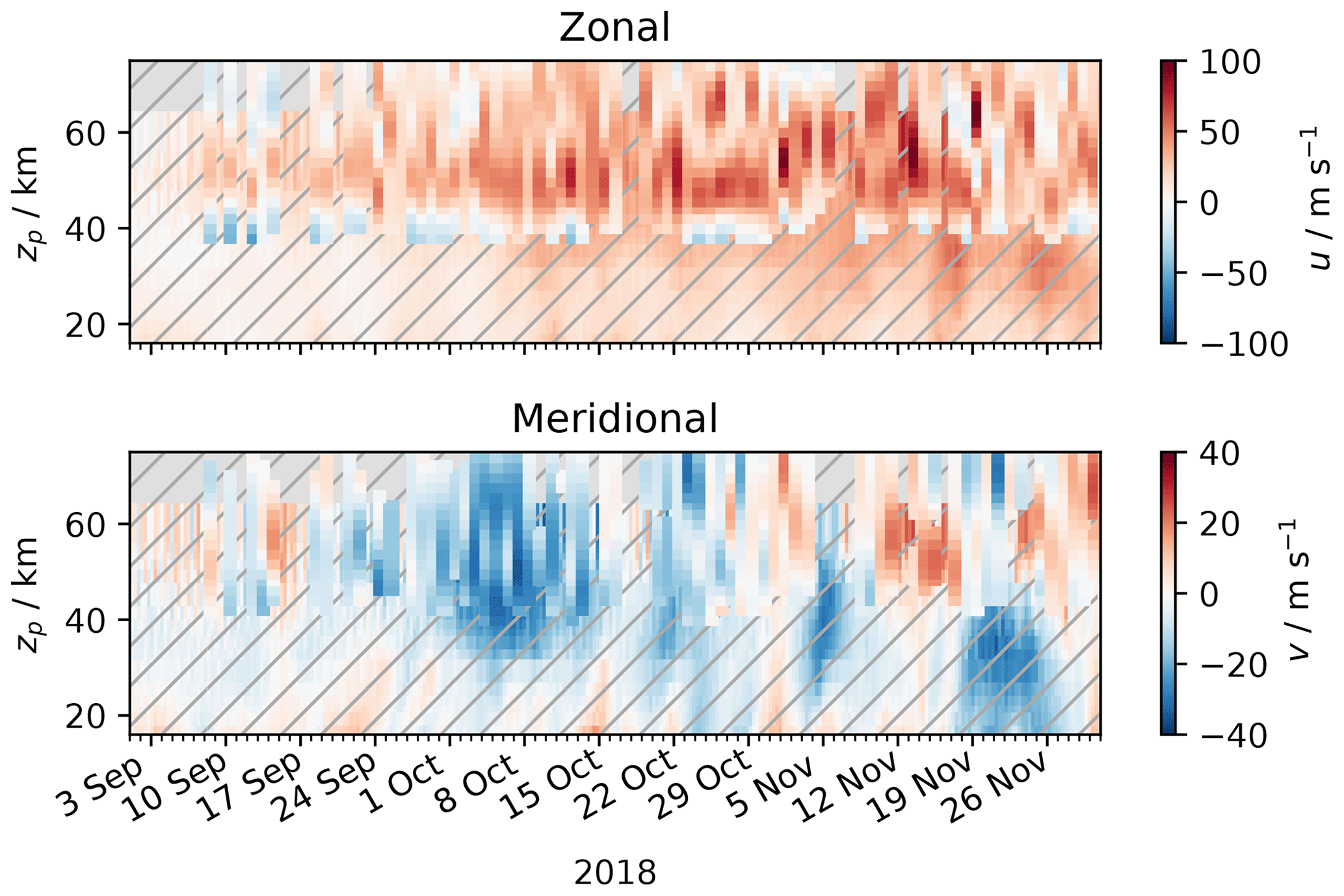
Figure 7 Background wind speed measured by WIRA-C complemented with MERRA-2 reanalysis data (hatching) for the arctic campaign. Note the different scales for the zonal and meridional components.

4.2 Results for the arctic campaign

From the ongoing arctic campaign in Andenes (ALOMAR), we selected September, October and November 2018 for our analysis. The measurement response during these months is between 0.8 and 1.2 between 42 and 62 km and between 0.7 and 1.3 between 39 and 69 km, and therefore it is acceptable for the whole altitude range we cover. We did not choose this period to start earlier because of the biannual wind reversal that took place just before September 2018 and, on the other end, we did not expand this period to December because of the major sudden stratospheric warming that took place in this winter (Schranz et al., 2019).

For this period, the meteorological situation is dominated by the fall transition in the stratosphere. The corresponding background wind field retrieval from WIRA-C is shown in Fig. 7. The campaign period starts at the end of summer with a weak eastward zonal jet between 45 and 55 km altitude, which evolves into a typical polar vortex until November covering nearly all observed altitudes from 40 to 70 km. Meridional winds are dominated by a southward flow at the beginning of the campaign period, which then reverses into a northward wind regime at the end of October. Both wind components indicate some variability due to waves on temporal scales of a few days; in particular, the meridional wind indicates an onset of the planetary wave activity towards the end of the observation period.

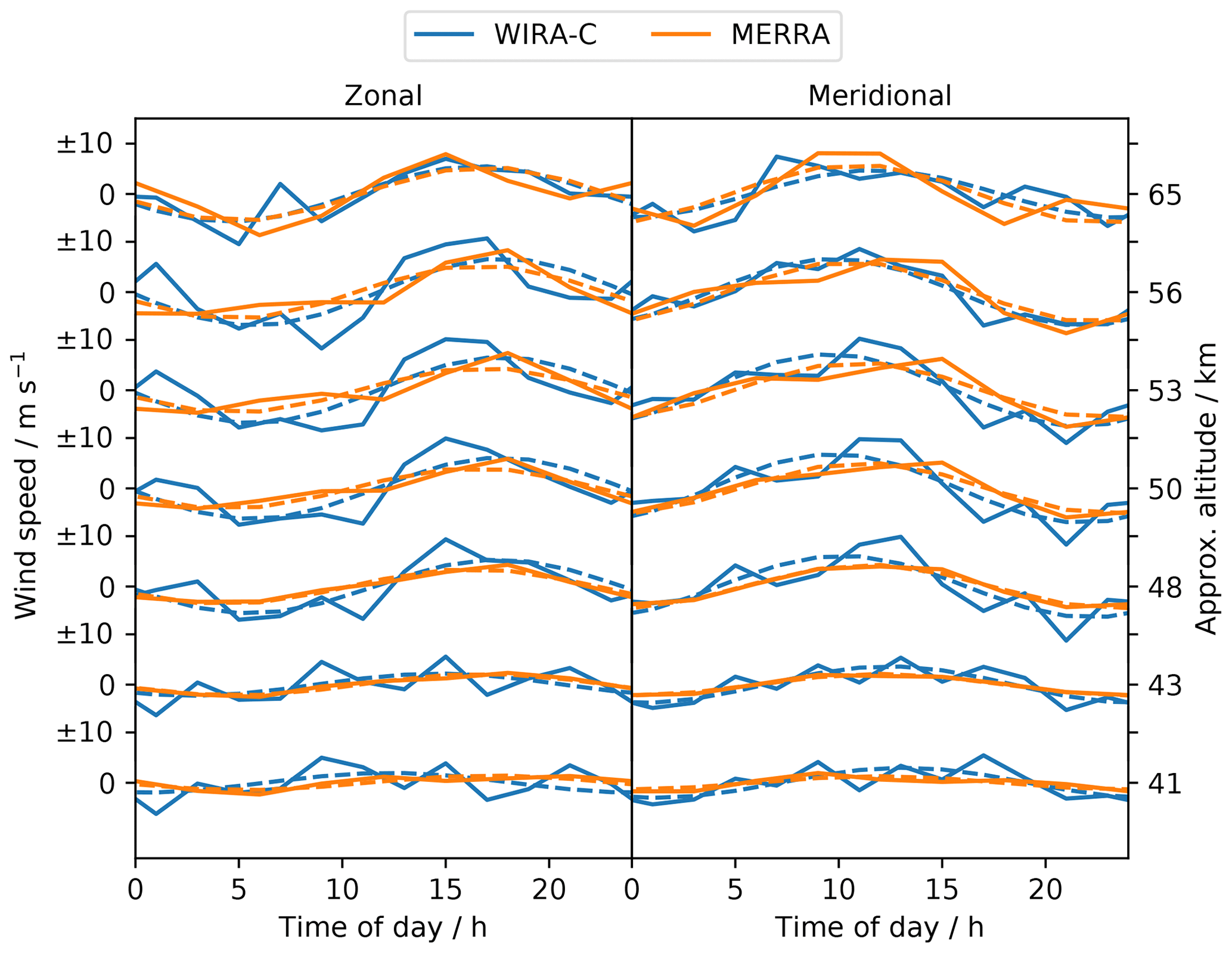
Figure 8 Mean daily cycle of zonal and meridional wind speeds at different altitudes for the 3 months during the arctic campaign from MERRA-2 and WIRA-C. Dashed lines indicate the best fit of the diurnal tide model.

Figure 8 shows the diurnal cycle, averaged over the 3 months during the arctic campaign. The reanalysis data are well fitted by our diurnal tide model at all altitudes, but the presence of a semi-diurnal component is indicated by the slight oscillation of the reanalysis data around the diurnal tide model fit. The WIRA-C measurements are well represented by the simple diurnal tide model, while containing some higher-frequency oscillations that could originate in higher mode oscillation as well as measurement noise.

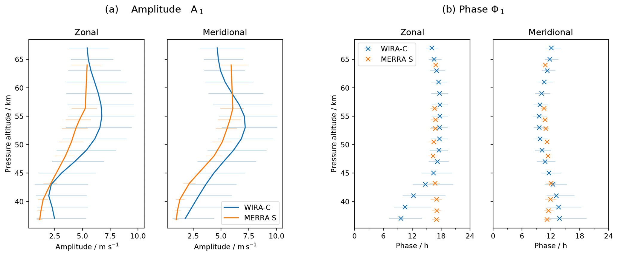
Figure 9 Amplitude and phase of mean daily cycle over 3 months from MERRA-2 reanalysis and WIRA-C measurements from the arctic campaign. Error bars indicate 95 % confidence limits. Phase is equivalent to solar time of maximum.

Figure 9 shows amplitude and phase profiles of the mean daily cycle of this period. Measurements and reanalysis mostly agree and show the same structure of the diurnal tidal amplitude and phase. Still as seen in Fig. 9a, WIRA-C measures a higher diurnal amplitude than the reanalysis suggests. Here, the offset in amplitude seems to be systematic since, for the most part, the profiles do not agree within their limits of confidence even though they show the same structure.

The phase of the mean daily cycle is shown in Fig. 9b. Both data sets show a situation with infinite vertical wavelength above 45 km. The maximum of the diurnal tide is around noon and 18:00 local time for the zonal and meridional components, respectively.

The phase difference between zonal and meridional components in the tri-monthly mean is shown in Fig. 4a. Above 45 km, the zonal tide leads the meridional tide by 6 h (90^∘ phase angle), as expected for the Northern Hemisphere. Below 45 km, the phase of the zonal component starts to deviate in the measurements and lags behind the meridional tide at approximately 40 km altitude.

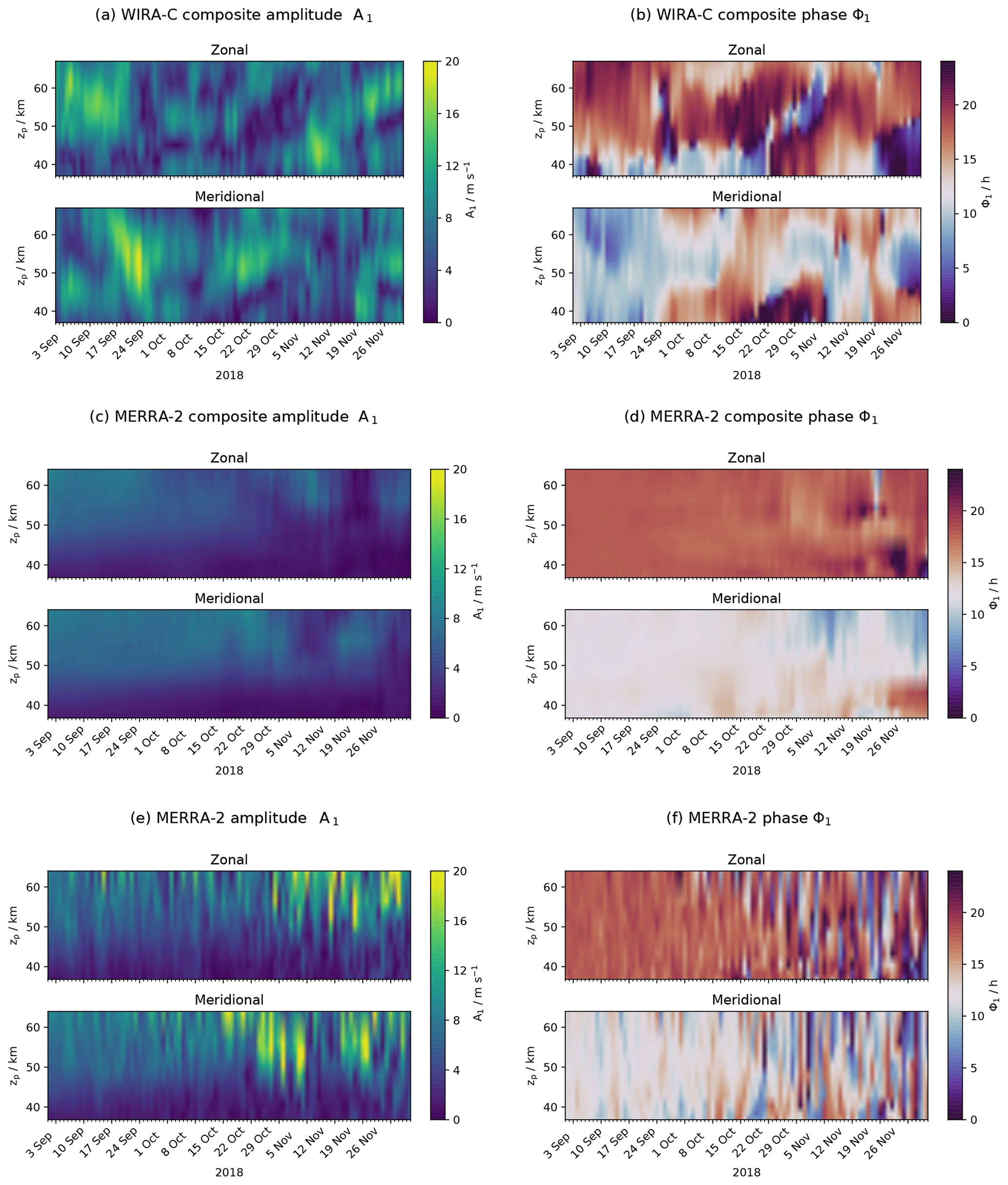
Figure 10 Amplitude and phase of the diurnal tide over 3 months from WIRA-C measurements (a, b), smoothed MERRA-2 reanalysis (c, d) and original MERRA-2 (e, f) during the arctic campaign at the ALOMAR observatory.

Figure 10 shows extracted amplitudes and phases of the diurnal tide for the arctic campaign over time and altitude. The panels on the left (Fig. 10a, c and e) show the diurnal tidal amplitude A₁ for the WIRA-C measurements and the MERRA-2 composite and original reanalysis, respectively. In the measurements, the diurnal tide is stronger in September than it is in October and reaches nearly 20 m s⁻¹ in the meridional component by the end of September. Again, this is most probably related to augmentation of tides by weaker background wind speed caused by the seasonal wind reversal that took place at the end of August to beginning of September 2018. But also during October and November, diurnal tidal amplitudes are quite strong, often up to or more than 15 m s⁻¹. This is different for the composite reanalysis data, where amplitudes are generally lower than 10 m s⁻¹. In the non-smoothed reanalysis data, tidal amplitudes of more than 15 m s⁻¹ are also reached.

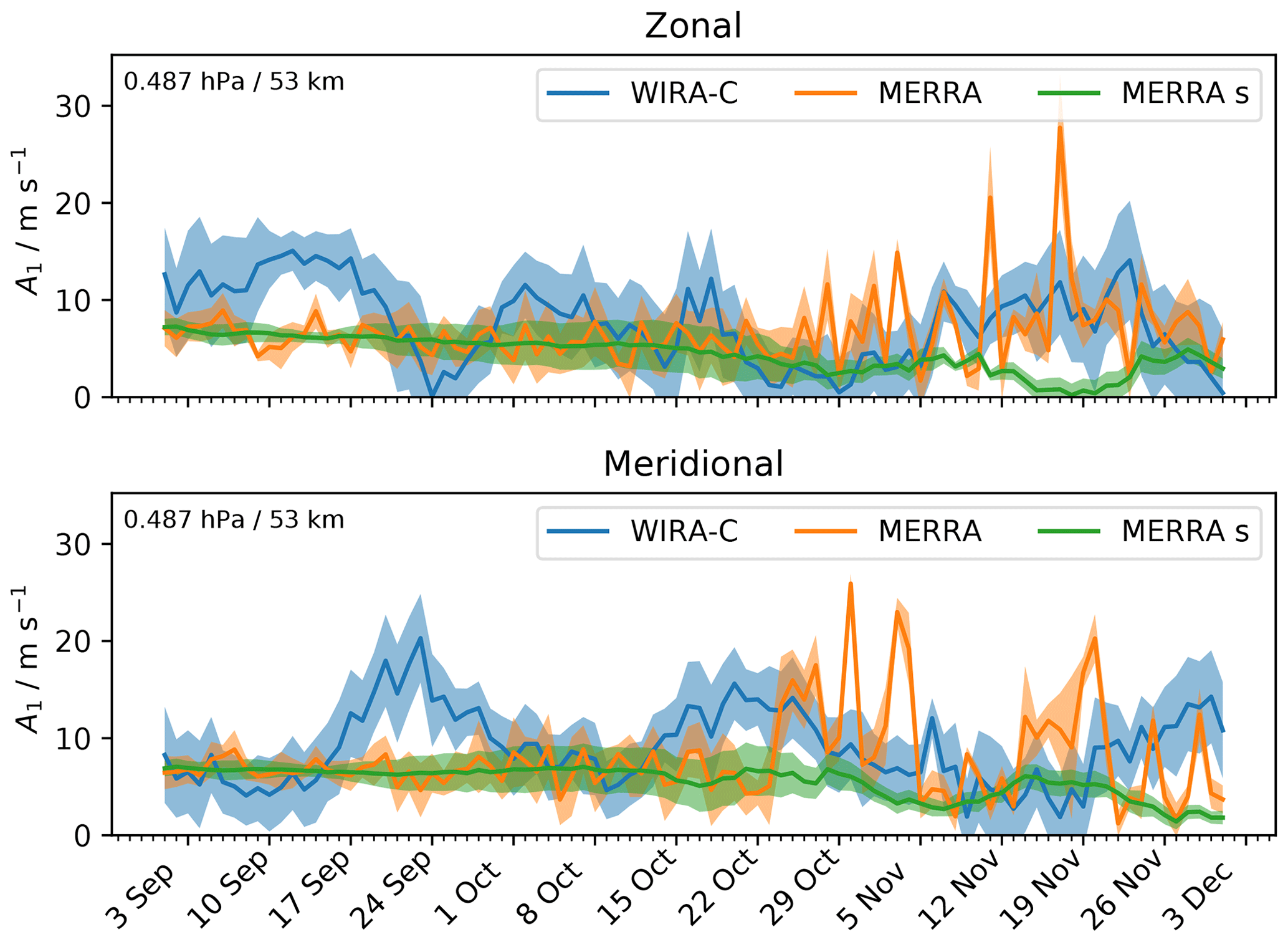
Figure 11 Time series of zonal and meridional diurnal tide amplitudes during the arctic campaign for measurements (WIRA-C), MERRA-2 reanalysis (MERRA) and reanalysis smoothed (MERRA s) at an altitude level of 53 km with corresponding errors of the model fit as shaded area.

The extracted diurnal tidal phase ϕ₁ is shown in Fig. 10b and d for the measurement and reanalysis, respectively. In general, the reanalysis shows a very stable phase with the maximum of the diurnal tide at noon local time for the zonal component and 18:00 local time for the meridional component. Only in November does the phase becomes more variable and expose some structure which might be related to the onset of planetary wave activity. This applies to the smoothed and original MERRA-2 data equally and is in strong contrast to the measurements, where the diurnal tidal phase is highly variable with time and altitude on the presented timescales. Because this time dependence is present in all composites with the same morphology, we partly attribute it to the intermittency of the diurnal tide, while the exact value of the phase might still be subject to noise.

As for the tropical campaign, we discuss the (13, 2) composite and provide a total of six composites in the Appendix (Figs. A3 and A4). Again we see the same morphology and time dependence of amplitude and phase in all composites. While the amplitude is less consistent among the composites due to noise, the phase is more robust.

Figure 11 shows the time series for one specific altitude level (53 km) and additionally shows the amplitudes of the original reanalysis data that have not been aggregated over multiple days. Especially in November, the original reanalysis data show a variability that is comparable or even stronger when compared to the measurements. By applying the aggregation, this variability is averaged out from the reanalysis data but not entirely from the WIRA-C measurements. If this variability comes from the atmosphere as opposed to instrumental noise, this would indicate that the coherence time of short-timescale disturbances of the diurnal tide might actually be longer than the reanalysis predicts. Notably, the measured amplitude features a disturbance around 24 September, where the zonal amplitude is close to zero and the meridional amplitude exhibits a maximum. Similar dynamics are not represented in the reanalysis data, not even in the (non-smoothed) original reanalysis data.

4.3 Summary

We presented measurements of the diurnal tide in the wind field in the stratosphere and lower mesosphere. To our knowledge, these are the first direct observations of tides in the wind field in the middle atmosphere (30 to 70 km) with ground-based instruments. In contrast to the standard time series retrievals applied in previous studies, we apply a composite analysis and superpose spectra for the same time of day over several days. This composite analysis enables us to resolve tidal structures in the wind field.

To investigate the results of our method, we applied our analysis to two 3-month periods from different campaigns: one from the Southern Hemisphere and one from the Northern Hemisphere.

The averaged data over the 3-month periods showed basic and well-known properties of the diurnal tide with different details for the Northern Hemisphere and Southern Hemisphere. Notably we observed an increasing amplitude with altitude, reasonable vertical wavelengths, and a 6 h (90^∘ phase angle) shift between zonal and meridional component with the leading component being different for the austral and boreal locations.

We compared our wind measurements to the MERRA-2 reanalysis, which has already been compared by Sakazaki et al. (2018) to other data sets in regards to tides in the temperature field. We find a good overall correspondence between reanalysis and measurements in the amplitude of the diurnal tide in the wind field and temporal evolution thereof. Further, the amplitude and phase profiles for the tri-monthly mean wind field correspond between the radiometer and the meteorological reanalysis, mostly within their uncertainties for the tropical campaign and with a small offset for the arctic campaign. While the phase of the diurnal tide is very stable in the reanalysis data, especially in the polar region and sometimes even stationary, we see a big temporal variation in the phase in our measurements, which persists among different composites.

Further, we presented a time series of the diurnal tidal amplitude and phase over two 3-month periods. We observed an augmented diurnal tide in the context of weak background wind speeds after seasonal wind reversals. Looking at shorter timescales, we observe strong temporal variability of the amplitudes and especially of the phase. Certainly, the time dependence of the diurnal tidal phase has to be investigated in further studies. Since we see the same time dependence in all our composites, we conclude that intermittent diurnal tides could be a possible explanation.

5 Conclusions

In summary, we find that reanalysis and measurements agree on the tidal component in the tri-monthly mean daily cycle. We conclude that the MERRA-2 reanalysis captures the amplitude and phase of the mean diurnal tide reasonably well when averaging over 3 months or longer. When looking at shorter timescales, obvious differences between model and measurements appear. We can explain some of the differences, like the augmented tide, in the context of weak background winds and also observe other notable differences like the variable phase in measurements that are not represented in the MERRA-2 product. Since the general morphology of the variable phase is the same among all composites, we conclude that it might be caused by actual atmospheric variability of the tide. While these intermittent structures are present to some extent in the reanalysis data as well, they are averaged out when we apply the 13 d smoothing that is equivalent to the composite of our measurement. A possible explanation would be that the coherence time of short-timescale disturbances of the diurnal tide is longer, and variability is in general stronger in reality than in the reanalysis model. On the other hand, our study is based on a composite analysis, and we assume that the diurnal tide is reasonably stationary during our 7 to 13 d window. Baumgarten and Stober (2019), based on temperature lidar observations with high temporal resolution, provide some evidence that tides can be highly variable and aggregation windows should be no longer than a few days. Further studies could develop more elaborate methods to extract tidal information from radiometer data and further constrain the uncertainty on the extracted parameters. Diurnal tide measurements from daylight-capable lidar or even from rocket campaigns would be a possible source of comparison data. Also other models, for example NAVGEM-HA, could provide further comparison data on different timescales.

In this study, we focused on the diurnal tidal component only. Future studies could as well address the semi-diurnal component using the same or different composites.

We required a stationary background and focused on selected periods which satisfy this condition. Further studies could investigate the necessity or this requirement and retrieve tides while taking a variable background into account.

Ground-based microwave radiometers are capable of measuring continuously over decades and can be deployed in tropical and polar latitudes with minimal maintenance and deployment effort. This makes these instruments very valuable to observe dynamics in the atmosphere, especially from 30 to 70 km altitude where observations are scarce. Since tidal waves on sub-seasonal and regional scales play an important role in the dynamics of the atmosphere, such observations are highly valuable.

Appendix A: Diurnal tide amplitude and phase for all composites

Figures A1, A2, A3 and A4 contain panels with the extracted amplitude and phase of the diurnal tide in the wind field for six different composites of the WIRA-C wind measurements. We refer to the different composites by (ΔD, ΔH), where ΔD indicates the number of days and ΔH the number of hours for the integration; the total integration time is thus given by ΔD × ΔH and ranges from 21 to 28 h for the presented composites. We select these six composites because they all have an integration time of around 24 h and provide different window lengths (7 to 13 d) and different resolutions (2 to 4 h).

Figure A1 Tropical campaign: amplitude of the diurnal tide for six different composites with a similar total integration time of 21 to 28 h ordered by window length.

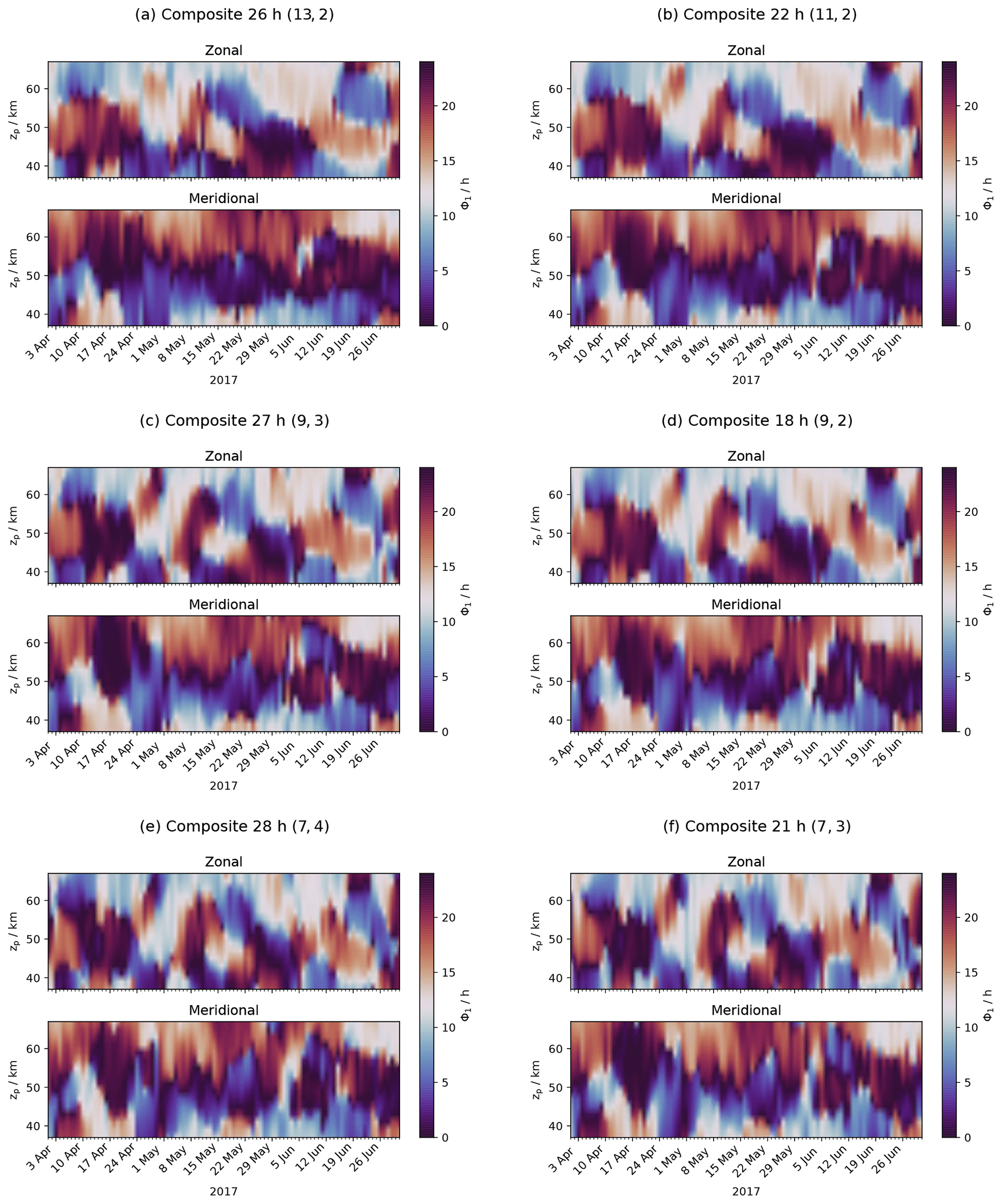
Figure A2 Tropical campaign: phase of the diurnal tide for six different composites with a similar total integration time of 21 to 28 h ordered by window length.

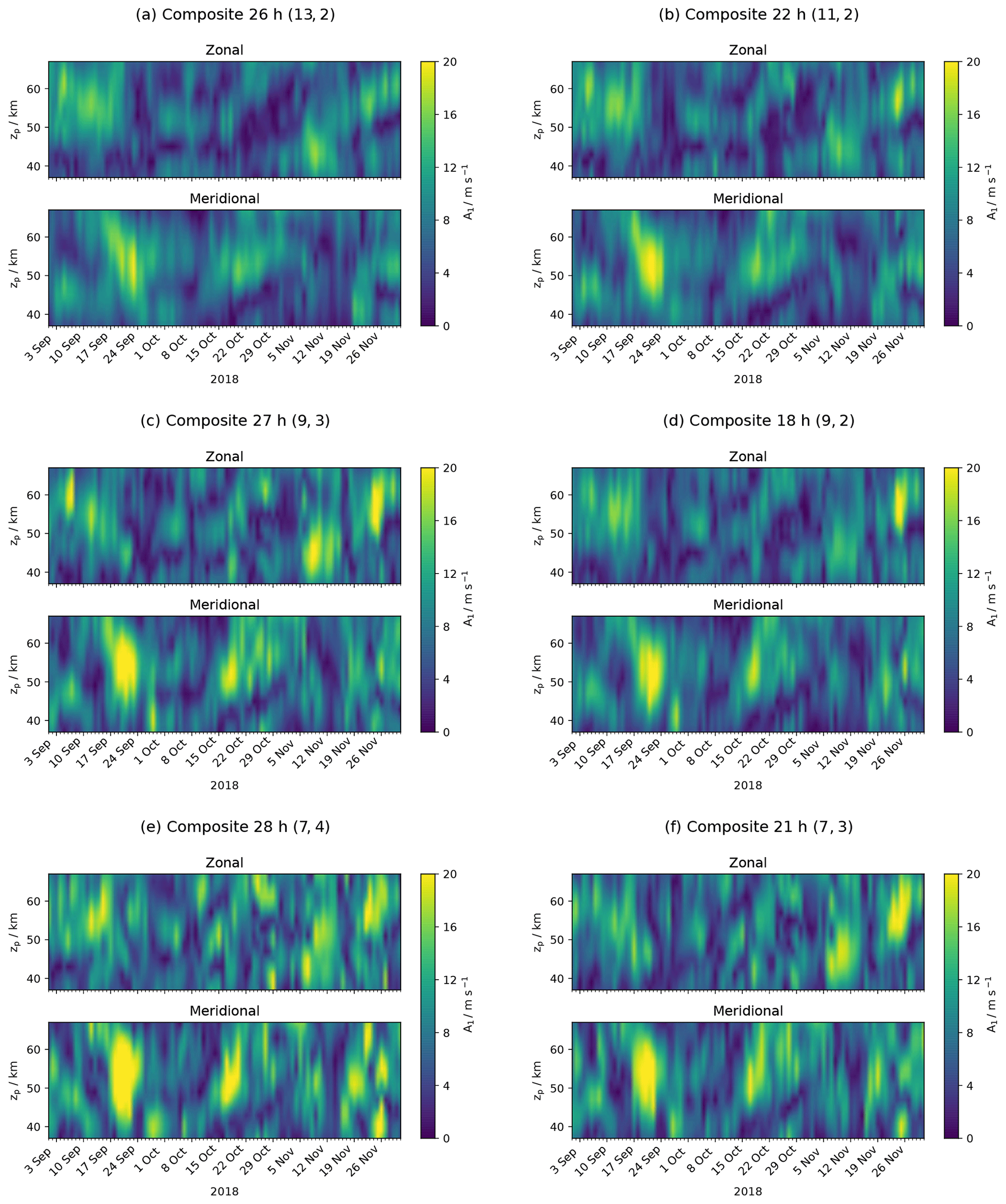
Figure A3 Arctic campaign: amplitude of the diurnal tide for six different composites with a similar total integration time of 21 to 28 h ordered by window length.

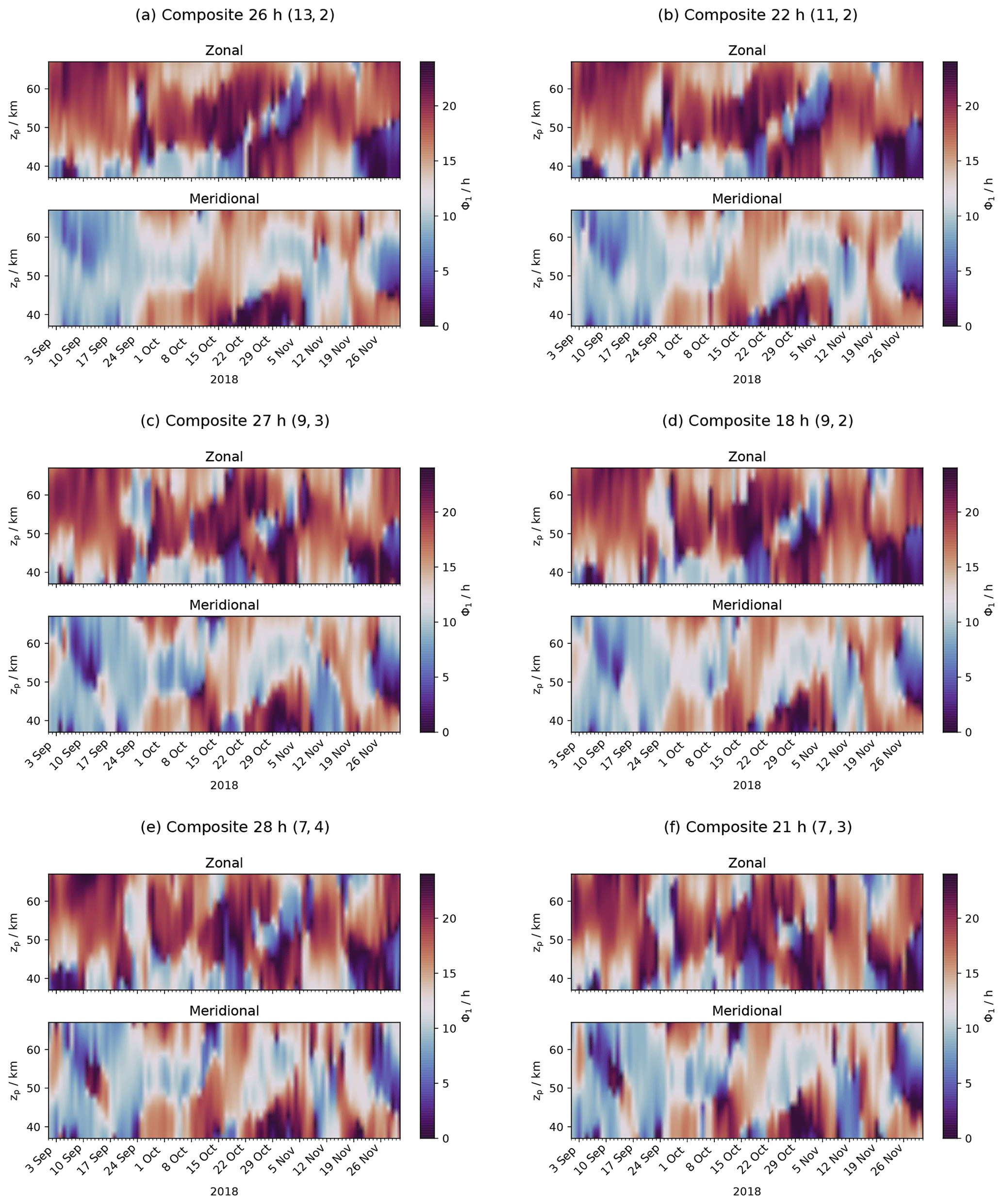
Figure A4 Arctic campaign: phase of the diurnal tide for six different composites with a similar total integration time of 21 to 28 h ordered by window length.