the Creative Commons Attribution 4.0 License.
the Creative Commons Attribution 4.0 License.
 | 26 Feb 2020
Photochemical modeling of molecular and atomic oxygen based on multiple nightglow emissions measured in situ during the Energy Transfer in the Oxygen Nightglow rocket campaign
Olexandr Lednyts'kyy
Christian von Savigny
Electronically excited states of molecular and atomic oxygen (six O2 and two O) were implemented in the proposed Multiple Airglow Chemistry (MAC) model as minor species coupled with each other as well as with the ground states of O2 and O to represent the photochemistry in the upper mesosphere and lower thermosphere (MLT) region. The MAC model combines chemical processes of well-known photochemical models related to identified O2 and O species and some additional processes. Concentrations of excited O2 and O species were retrieved using the MAC model on the basis of the multiple nightglow emissions measured in situ during the Energy Transfer in the Oxygen Nightglow (ETON) rocket campaign. The proposed retrieval procedure to obtain the concentrations of these minor species in the MLT region is implemented by avoiding a priori data sets. Unknown and poorly constrained reaction rates were tuned, and the reaction rates of the well-known models were updated with the MAC model by comparing in situ and evaluated emission profiles as well as in situ and retrieved O concentration profiles. As a result, precursors of O2 and O species responsible for the transitions considered in the MAC model are identified and validated.
- Article
(1973 KB) - Full-text XML
- BibTeX
- EndNote


Airglow is a permanent global atmospheric phenomenon that can hardly be seen without appropriate instruments. Ångström (1869) used such instruments and observed the green line emission at 557.7 nm in the nightglow (airglow at night) from the Earth's surface in 1868 for the first time. The origin of airglow was considered to be the same as the origin of aurora, a sporadic arc-like atmospheric phenomenon that has fascinated numerous spectators for many thousands of years.
Table 1Relevant optical transitions of terrestrial airglow in the Earth's atmosphere. Emissions (see the column labeled “Emission”) observed in the wavelength range shown in the λ column are denoted by abbreviations (see the column labeled “Ident.”). Typical intensity values of an integrated (limb) emission rate profile are given for nightglow (see the “Int.” column before the comma) and, if available, dayglow (see the “Int.”column after the comma). The altitudes of the corresponding emission rate peaks are shown in the column labeled “Alt.”. Atomic oxygen emissions are denoted by abbreviations as follows. GrL – the green line emission at 557.7 nm, ReL – the red line emissions at 630.0 and 636.4 nm, UVL and UVL∗ – the ultraviolet line emissions at 297.2 and 295.8 nm, respectively. Molecular oxygen emissions are denoted by abbreviations as follows. IRAtm – the infrared atmospheric band emission at 1270 nm, Atm – the atmospheric band emission at 761.9 nm, Nox – the atmospheric band emission at 1908 nm, HzI – the Herzberg I band emissions, BG – the Broida–Gaydon band emissions, Cha – the Chamberlain band emissions, HzIII – the Herzberg III band emissions, HzII – the Herzberg II band emissions, cbK – the new system band emissions measured using the Keck I/II instrument (Slanger et al., 2004a), RJ – the Richards–Johnson band emissions. References are marked with upper indices as follows: sc – Slanger and Copeland (2003), mc – McConkey et al. (1966), na – Nagy et al. (2008), md – McDade (1998), kh – Khomich et al. (2008).
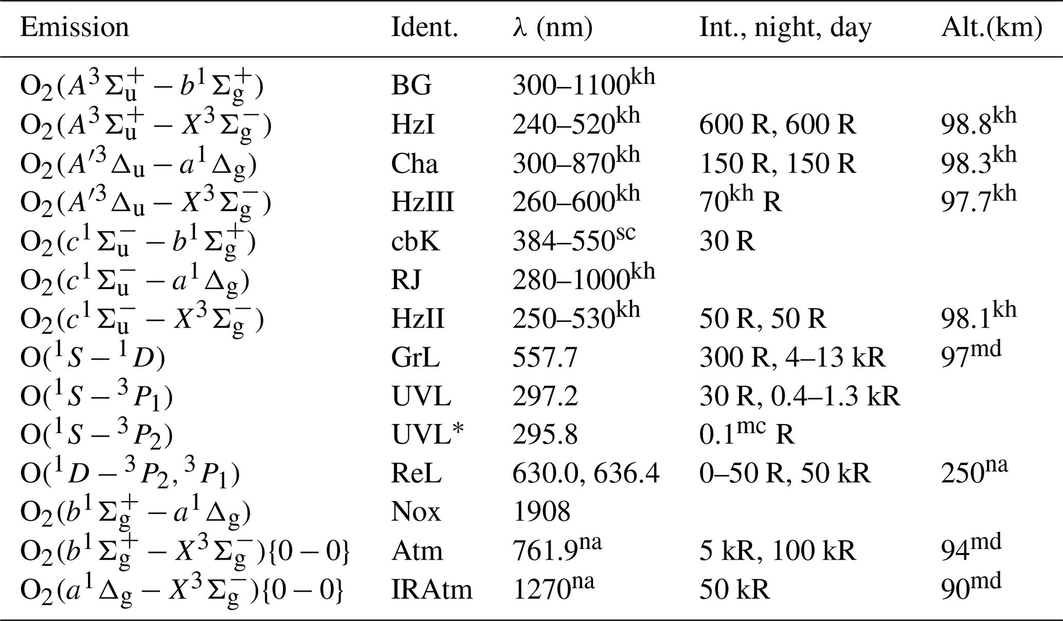
Table 1 provides an overview of relatively strong airglow emissions detected in the upper mesosphere and lower thermosphere (MLT) in situ and remotely. The Energy Transfer in the Oxygen Nightglow (ETON) rocket campaign, conducted in March 1982 and discussed in Sect. 2, was conceptualized to obtain in situ profiles of airglow volume emission rates (VERs) and other atmospheric parameters like atomic oxygen (O) in the ground state (O(3P)) to verify and validate photochemical models describing airglow.
O(3P) is a chemically active MLT trace gas and a critical component for the energy budget of the MLT region. O(3P) is also required to retrieve carbon dioxide (CO2) concentrations as well as profiles of kinetic temperature and pressure (Remsberg et al., 2008; García-Comas et al., 2008; Rezac et al., 2015). In addition, O(3P) is also a major component of the neutral bath gas in the upper thermosphere, significantly contributing to the nighttime ionosphere (Shematovich et al., 2011; Wei et al., 2014).
The transition O(1S−1D) from the second excited O state (O(1S)) to the first one (O(1D)) is detected as the 557.7 nm green line emission. The Chapman excitation scheme and the Barth excitation transfer scheme were proposed in 1931 and 1962, respectively, to explain the origin of the green line emission in the MLT. The Chapman excitation scheme considers a collision of two O(3P) atoms and a third body represented by O(3P) to produce O(1S) (Chapman, 1931, 1937). The Barth excitation transfer scheme considers (1) a collision of two O(3P) atoms and a third body represented by an abundant molecule, e.g., molecular nitrogen (N2) and oxygen (O2), to produce O2 in an unidentified excited state () as well as (2) an energy transfer from to O(3P) so that O(1S) is produced (Bates, 1979). Comparing both excitation schemes, Bates (1979) interpreted the Chapman excitation process to consist of four steps as follows: (1) two O(3P) atoms collide, (2) creating a common surface of potential energy of, presumably, an electronically excited O2 molecule in the upper Herzberg state (Greer et al., 1987); (3) after its collision with a third O(3P) atom (4) one vibrationally excited O2 molecule and one O(1S) atom are created. One of the differences between the Chapman and Barth excitation schemes is the kind of third body, which is an O(3P) atom or an abundant molecule in the MLT, respectively. The energy transfer considered in the Barth scheme includes acting as the O(1S) precursor, but the Chapman scheme does not include it. Photochemical models proposed to implement the Chapman and Barth schemes are hereafter referred to as the first (one-step) and the second (two-step) type, respectively.
Airglow emissions are very complex atmospheric phenomena so that photochemical models are often proposed to derive unknown or poorly constrained reaction rates, which can be backed up by reaction rates determined in the laboratory with the use of the Stern–Volmer method. The Stern–Volmer method is applied to analyze concentration-dependent kinetics in a homogeneous system, to which a quencher was added (Lakowicz, 2006). According to the Stern–Volmer method, excited and quenching chemical species are considered in a system of a few photochemical reactions so that steady-state methods can be applied to describe emissions. Then measurements of the lifetimes or concentrations of emitting species enable the determination of the true pseudo-first-order decay required to calculate the rate coefficient of the considered quenching reaction. However, the same values of the pseudo-first-order decay rate are possible for both the dynamic quenching and the static quenching at the given temperature (Lakowicz, 2006). Dynamic quenching reduces the apparent fluorescent lifetime, while static quenching rather reduces the apparent concentration of fluorescent species during inelastic collisions (Lakowicz, 2006). Unfortunately, the reactive collisions responsible for static quenching are not so well understood compared to the products of dynamic quenching and can introduce difficulties calculating the rate coefficient of the considered quenching reaction.
Table 2Processes of the O(1S) nightglow model with as the O(1S) precursor were proposed by McDade et al. (1986) and modified by Lednyts'kyy et al. (2015) according to Gobbi et al. (1992) and Semenov (1997). Odd oxygen processes related to O2(b) were described with the well-known quadratic equation of McDade et al. (1986). Odd oxygen processes related to O(1S) were described by two models. The first model excluded two processes, Rg1.2 and Rg2.1, and resulted in the well-known cubic Eq. (2) of McDade et al. (1986). The second model included two processes, Rg1.2 and Rg2.1, and resulted in the extended cubic Eq. (3) of Lednyts'kyy et al. (2015). The processes marked with a character P were not considered in proposing the MAC model but were used in the first step (prior) retrieval of [O(3P)]. Odd oxygen processes related to O(1S) represent the two-step Barth transfer scheme (see reactions Rv1.1–2, Rv2.1 and the resulting reaction Rg3.0) accompanied by quenching. The symbolic representation of the reaction rates shown above the arrows in the second column of this table was adopted from Khomich et al. (2008) and used in Sect. 3.1. The symbolic representation shown in the third column of this table was used by Lednyts'kyy et al. (2015). For instance, the reaction rate βO (Khomich et al., 2008) corresponds to (Lednyts'kyy and von Savigny, 2016), (Khomich et al., 2008) corresponds to (Lednyts'kyy and von Savigny, 2016), A558 (Khomich et al., 2008) corresponds to (Lednyts'kyy and von Savigny, 2016) and (Khomich et al., 2008) corresponds to (Lednyts'kyy and von Savigny, 2016). Processes marked with a character P were used at the prior retrieval steps applied to calculate [O(1S)] (see Sect. A1.1) and [O(3P)] (see Sect. 3.1 and 3.5).
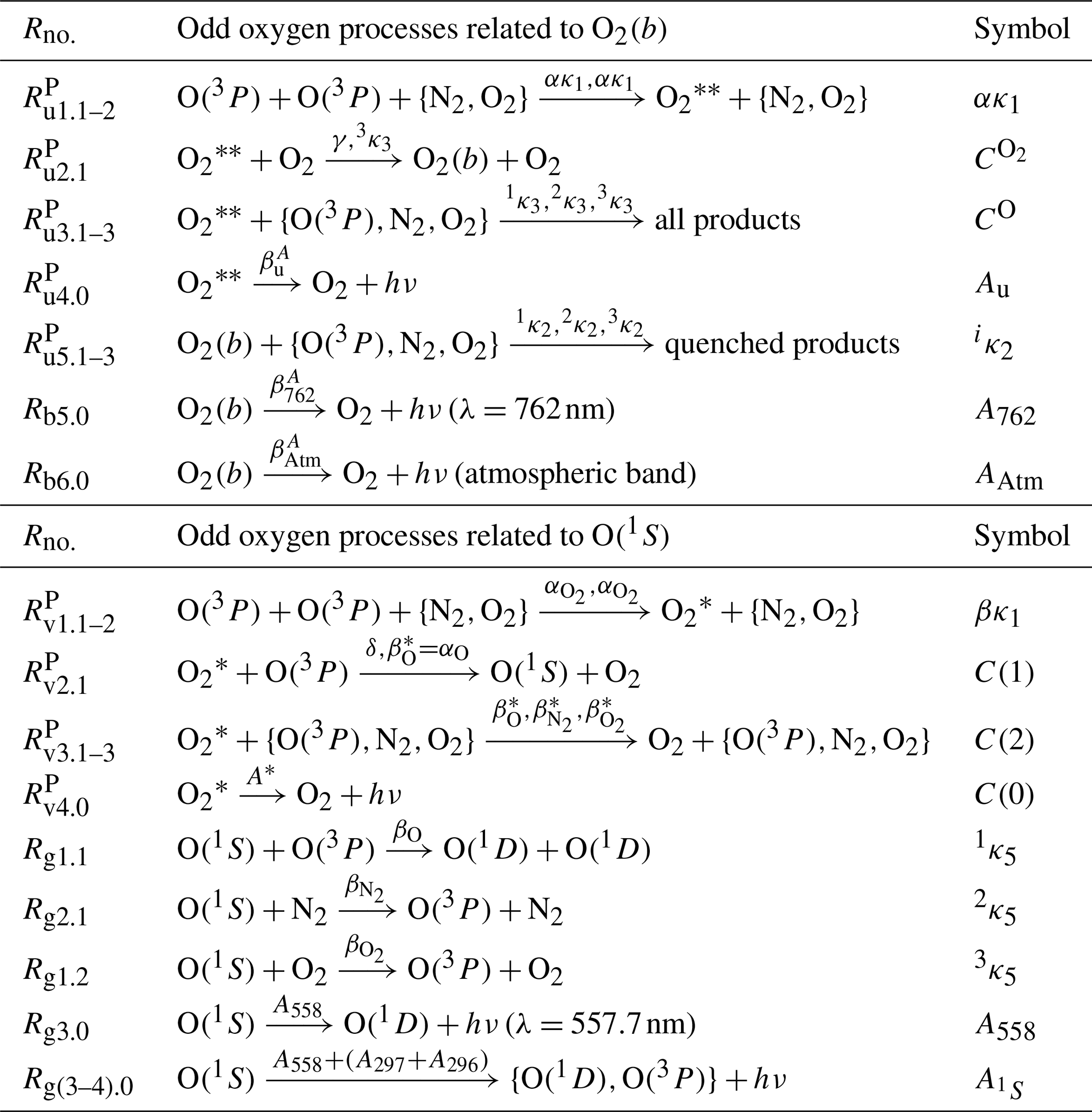
If no more than one emission, e.g., VER{O(1S−1D)} in McDade et al. (1986), is considered in the model of the second type then the resulting steady-state chemical balance equation (hereafter referred to as the continuity equation) is of the third degree with respect to [O(3P)], and the respective solutions can be easily interpreted. As for the O2(b−X) transition, McDade et al. (1986) developed photochemical models of the first and second types to describe transitions from O2(b) (the second electronically excited state of molecular oxygen, O2) to O2(X) (the electronic ground state of O2). This transition in the atmospheric band was measured in situ in the Earth's atmosphere during the ETON campaign to retrieve VER{O2(b−X)}. The model of the second type developed by McDade et al. (1986) with the O2(b) precursor and O2(b) was proposed to explain nonlinearities detected in quenching processes simulated by using the model of the first type developed by McDade et al. (1986) with O2(b) only. McDade et al. (1986) used known reaction rates and tuned poorly constrained reaction rates of these quenching processes in the atmosphere so that simulated profiles match the in situ observations. The processes considered in the models of the first and second types provided in Table 2 were developed by McDade et al. (1986) to describe atmospheric airglow emissions and to verify the obtained results in the laboratory using the Stern–Volmer relationship.
The total number of reactions considered in the models of López-González et al. (1992b) and McDade et al. (1986) with the O(1S) precursor () and O(1S) was limited to 10, and these reactions are separated in two groups according to the Barth excitation transfer scheme. A full overview of these reactions including O2 in an unidentified excited state () is not provided in this short overview except for two reactions. Specifically, López-González et al. (1992b) considered the reaction , which McDade et al. (1986) did not consider. But McDade et al. (1986) considered the reaction , which López-González et al. (1992b) did not consider. Possible reasons to limit the list of all possible reactions in these models are as follows: (1) the Barth excitation transfer scheme can be represented by the most important (e.g., 10) reactions, (2) the system of a few reactions can be easily represented by a low degree polynomial equation regarding [O(3P)], (3) additional reactions would introduce difficulties to derive their rates, which are sometimes treated as ratios of reaction rates and tuned as empirical coefficients, and (4) the choice of approaches applied to derive empirical coefficients is limited depending on the considered reactions, e.g., compare approaches applied by McDade et al. (1986) and López-González et al. (1992b).
These reasons limit the applicability of the mentioned methods used to analyze laboratory results and atmospheric measurements, which are usually studied without propagation in time. The computational simulation of a chemical kinetics system enables the study of the time evolution of chemical species using the ordinary differential equation (ODE) system matrix and initial conditions; see, e.g., Sandu and Sander (2006) for an overview of zero-dimensional box models developed to integrate ODEs numerically in time. Unfortunately, computer modeling depends on the a priori data sets used to initialize a box model. In situ atmospheric measurements may be influenced by gravity waves and atmospheric tides at particular moments in time, which hinders the use of box models on the basis of such measurements. The current article studies MLT photochemistry on the basis of the in situ ETON measurements using steady-state continuity equations, i.e., without propagation in time and without a priori data sets.
The ETON multiple airglow emissions described in Sect. 2 can be applied simultaneously in the model proposed in this study to decrease uncertainties when tuning unknown and poorly constrained reaction rates with the use of the verification and validation procedures.
Torr et al. (1985) appear to be the first to consider multiple emissions in a model with several O2 states based on observational data from the shuttle Spacelab 1. In fact, these data sets were extremely scattered in time and place and might have stopped Torr et al. (1985) from combining identified O2 states in one model. Instead, they considered a number of photochemical models with some excited O2 states in each model so that all discussed excited O2 states appeared to be uncoupled with each other. Note that Torr et al. (1985) also considered O2(c) to be the O(1S) precursor, as suggested by Greer et al. (1981), and applied the O(1S) quenching with O2(a) according to Bates (1981) and Kenner and Ogryzlo (1982).
In summary, the current investigation was conducted to study the following topics regarding the new photochemical model proposed here: (1) processes of O(1S) formation and quenching (see Sect. 3.1), (2) processes including identified O2 states (see Sect. 3.2.1, 3.2.2 and 3.3), and (3) the O(1S) precursor represented by one O2 state or a group of them (see Sect. 4.3).
The O(3P) retrieval scheme was proposed to be solved in subsequent steps as described in Appendix A on the basis of multiple airglow emission profiles as discussed by Lednyts'kyy and von Savigny (2016) and Lednyts'kyy et al. (2018). Note that a priori data are not required to initiate calculations with the MAC model. Concentrations of O2 in higher excited states are calculated in earlier steps of the retrieval procedure and are used to calculate concentrations of O2 in lower excited states in the following steps. It should be noted that a limited number of multiple airglow emissions available from the ETON measurements or other sources can also be applied to retrieve [O(3P)] values at some of the mentioned retrieval steps; see Sects. 2 and 5 for details.
In situ measurements obtained during the Energy Transfer in the Oxygen Nightglow (ETON) campaign and simulations using the most recent version of the MSIS (Mass Spectrometer Incoherent Scatter) semi-empirical model are the focus of this section.
Volume emission rates (VERs) of the nightglow emissions measured in situ during the ETON campaign and the corresponding statistical errors provided by Greer et al. (1986) were used in this study. The ETON campaign is comprised of measurements obtained during coordinated launches of seven sounding rockets at South Uist (∼ 57∘16′ N, ∼ 7∘19′ W) in Scotland in the westerly direction on 23 March 1982 from ∼21:27 to ∼ 23:55 UT (Greer et al., 1986, 1987).
All VER profiles considered in the MAC model were measured during flights of two ETON rockets. The infrared atmospheric band emission at 1.27 µm was measured with a photometer aboard only one ETON rocket: the P227H rocket launched at ∼22:11 UT. The Herzberg I and atmospheric band emissions at 320 and 761.9 nm, respectively, were also measured by the P227H rocket. The P229H rocket was launched at ∼22:58 UT right after the P227H rocket and provided measurements of the Herzberg I, Chamberlain and atmospheric band emissions at 330, 370 and 761.9 nm, respectively, as well as the oxygen green line emission at 557.7 nm. It should be noted that the Chamberlain band emissions were measured by the P229H rocket only. The absolute accuracy of ±20 % in VER peak values for the infrared atmospheric band emissions and better than ±10 % in other wavelength ranges (Greer et al., 1986) introduces uncertainties in the [O(3P)] retrievals.
In situ measurements of atomic oxygen (O) concentrations ([O]) in the ground state [O(3P)] were carried out by the P232H and P234H rockets launched at ∼21:49 and 55 UT, respectively. [O(3P)] values were determined directly using the resonance fluorescence and absorption technique at ∼130 nm (Greer et al., 1986) and were interpolated for the launch time of the other ETON rockets. The statistical (and the systematic) error was less than about ±10 % (and about ±30 %) at about 100 km (where peak [O(3P)] values were measured) and increased up to ±50 % (and about ±20 %) at other altitudes (where low [O(3P)] values were measured) (Greer et al., 1986).
The most recent version of the MSIS model, NRLMSISE-00 (Naval Research Laboratory MSIS Extended, 2000; see Picone et al., 2002), was used to obtain the following input parameters required to run the MAC model: temperature (T), molecular nitrogen concentrations ([N2]) and [O2]. Because the highest number of O2 and O transitions were sounded by the P229H rocket, the time of in situ measurements obtained by the P229H rocket at ∼97 km over South Uist in Scotland was specified for the NRLMSISE-00 model. It should be mentioned that McDade et al. (1986) developed the well-known cubic equation deriving empirical coefficients using the MSIS-83 model (Hedin, 1983) that is no longer available.
The input parameters required to run the established models and the proposed MAC model are profiles of T, [N2], [O2] and VER values. The following abbreviations of in situ VER profiles are used in this study: VER{O2(A−X)} (Herzberg I band, HzI), VER (Chamberlain band, Cha), VER{O2(b−X)} (atmospheric band, Atm), VER{O(1S−1D)} (green line, GrL) and VER{O2(a−X)} (infrared atmospheric band, IRAtm). Some of the O2 transitions listed in Table 1 correspond to these VER profiles. Note that the other listed O2 transitions were also considered in the proposed MAC model; see Sect. 3.3 for details. It is worth mentioning that all of these O2 transitions were measured remotely using the instrument SCIAMACHY (SCanning Imaging Absorption spectroMeter for Atmospheric CHartographY) aboard the satellite ENVISAT (ENVIronmental SATellite) launched by the European Space Agency (Burrows et al., 1995; Bovensmann et al., 1999).
It should be mentioned that Lednyts'kyy and von Savigny (2016) tuned unknown or poorly constrained reaction rates considered in the MAC model on the basis of the data sets obtained during the ETON campaign. The corresponding reaction rates are shown in Tables 8, 9, 10 and 11. Then, the MAC model was applied by Lednyts'kyy et al. (2019) on the basis of data sets obtained during the following three campaigns: the WADIS-2 (WAve propagation and DISsipation in the middle atmosphere), WAVE2000 (WAVes in airglow structures Experiment, 2000) and WAVE2004. The WADIS-2 rocket provided all data sets required to retrieve [O(3P)] values. Data sets measured in situ with rockets launched during the WAVE2000 and WAVE2004 campaigns were combined with the collocated data sets measured remotely. Convincing retrieval results enabled the validation of tuned reaction rates and calculations carried out with the MAC model.
3.1 The O(1S) nightglow model with as the O(1S) precursor
The established photochemical models of McDade et al. (1986), Gobbi et al. (1992) and Semenov (1997) related to the oxygen green line emission are described briefly in this section; see Lednyts'kyy et al. (2015) for details.
McDade et al. (1986) considered the processes provided in Table 2 that resulted in two photochemical models according to the two-step Barth excitation transfer scheme implemented in each model and involving precursors of O2(b) and O(1S), respectively. McDade et al. (1986) also implemented one model according to the one-step excitation scheme and related to O2(b), but excluding the O2(b) precursor. Both models related to O2(b) were used to retrieve [O(3P)] on the basis of the volume emission rates (VERs) of the atmospheric band emissions. All processes of the O2(b) model involving the O2(b) precursor are provided in the upper part of Table 2. In fact, reactions related to (, and ) are absent in the model implemented without the O2(b) precursor. The model implemented without the O2(b) precursor exhibits nonlinearities in quenching processes, but the model implemented with the O2(b) precursor () does not result in such nonlinearities (McDade et al., 1986). Note that McDade et al. (1986) described the green line emission considering the O(1S) precursor according to the Barth excitation transfer scheme. In fact, the well-known quadratic equation resulting from the model with the O2(b) precursor and the well-known cubic equation resulting from the model with the O(1S) precursor were concluded by McDade et al. (1986) to be favorable compared to models based on the one-step (Chapman) excitation scheme. It is worth mentioning that Grygalashvyly et al. (2019) proposed a model combining the Chapman and Barth excitation schemes, which were implemented in both O2(b) models of McDade et al. (1986) separately. Applying self-consistent data sets (see Sect. 2) and fitting retrieved data sets, Grygalashvyly et al. (2019) applied the methods of McDade et al. (1986) to derive new values of empirical coefficients, which were initially derived by McDade et al. (1986) for the well-known quadratic equation. The newly derived coefficients were preferred by Grygalashvyly et al. (2019) to be applied in their model.
The well-known cubic equation of McDade et al. (1986) provided below in the full form was used here to retrieve [O(3P)] on the basis of VER of the green line emission (VER558, also referred to as VER{O(1S−1D)}).
The cubic equation in the full form is as follows:
where R≈4 represents the mean [N2]∕[O2] ratio valid in the altitude range 80–120 km according to McDade et al. (1986). All reaction rates shown in Eq. (1) correspond to the ones provided in the lower part of Table 2. Ratios of some of these reaction rate values were derived by McDade et al. (1986) (see the empirical coefficients in Eq. (2) of Murtagh et al., 1990) on the basis of the ETON in situ measurements as well as simulated temperature, [N2] and [O2] profiles.
The well-known cubic equation and the derived empirical coefficients in particular were verified by Murtagh et al. (1990), who provided the well-known cubic equation in the short form as follows:
where the rate coefficient of the Rg1.2 reaction provided in Table 2 is molec−1 cm3 s−1, the Einstein coefficients of the reactions Rg3.0 and Rg(3–4).0 are A558=1.18 s−1 and s−1, and the rate βκ1 of the three-body recombination reaction is the product of molec−2 cm6 s−1 and an empirical β value. The reaction refers to the first step of the Barth excitation transfer scheme describing the production of , the O(1S) precursor. The rates , and of the reactions describe the quenching. The reaction with the rate value , where δ is an empirical value, refers to the second step of the Barth excitation transfer scheme, resulting in O(1S)+O2.
The values of the empirical coefficients C(0), C(1) and C(2) are equal to 0, 211 and 15, respectively, and these values are used in this study for retrievals using the well-known cubic equation according to Murtagh et al. (1990). Note that these empirical coefficients were derived by McDade et al. (1986) using semi-empirical models, including MSIS-83 (Hedin, 1983), that are no longer available. The NRLMSISE-00 model mentioned in Sect. 2 is used in this study to simulate temperature, [N2] and [O2] profiles. McDade et al. (1986) used various available models that resulted in other values of temperature, [N2] and [O2] profiles and different values of the empirical coefficients. The lowest obtained values of C(0), C(1) and C(2) from all obtained ones, which are related to the O(1S) precursor, were found by McDade et al. (1986) to be equal to 13±4, 183±10 and 9±3, respectively, and their highest values were found to be 23±9, 224±20 and 17±3, respectively.
Gobbi et al. (1992) suggested that processes of the enhanced O(1S) quenching with O(3P) and N2 should also be considered in the well-known Eq. (2). The extended cubic equation provided by Gobbi et al. (1992) is as follows:
where the rate coefficients corresponding to the reactions Rg1.1, Rg2.1 and Rg1.2 are molec−1 cm3 s−1, molec−1 cm3 s−1 and molec−1 cm3 s−1, respectively. The other coefficients are shown and described for Eq. (2). The photochemical model resulting in the extended cubic equation is hereafter referred to as the G model in short according to the surname of the first author in Gobbi et al. (1992), who proposed this model.
The O(1S) quenching with N2 is not effective according to Atkinson and Welge (1972) because the 2κ5 value is 5 orders lower than the 3κ5 value of the O(1S) quenching with O2. Therefore, the O(1S) quenching with N2 was neglected (2κ5=0) by Semenov (1997), who considered a relatively high 1κ5 value of molec−1 cm3 s−1 compared to the 1κ5 value of molec−1 cm3 s−1 used by Gobbi et al. (1992). The low 1κ5 value was obtained theoretically by Krauss and Neumann (1975) and approved experimentally by Kenner and Ogryzlo (1982). However, Johnston and Broadfoot (1993) and a number of other scientists including Khomich et al. (2008) used the high 1κ5 value.
Semenov (1997) developed the photochemical model that resulted in the cubic equation as follows:
where and ; see the notation of process rates provided in Table 2. The notation of other process rates shows that Eq. (4) can be transformed into Eq. (3) by using , , and 2κ5=0 molec−1 cm3 s−1.
The O(1S) quenching with O2(a) is very effective according to Bates (1981) and Kenner and Ogryzlo (1982), but the direct inclusion of O2(a) in Eq. (3) would increase its order so that the number of the obtained solutions would be very complicated to interpret. Therefore, the high 1κ5 value of the O(1S) quenching with O(3P) was adopted by Lednyts'kyy et al. (2015) in order to implicitly include the O(1S) quenching with O2(a) and to keep the order of the polynomial in Eq. (3). In this context it is worth mentioning that – according to Garcia and Solomon (1985) – O(1S) quenching reactions are not completely established. The direct correspondence of Eq. (4) (with defined empirical coefficients C(0), C(1) and C(2)) and Eq. (3) enabled the specification of how the relationship between values of [O(3P)] and VER558 can be used to solve both Eqs. (4) and (3) by applying the analytical method of Semenov (1997).
The well-known cubic Eq. (2) represents the reduced form of the extended Eq. (3). Indeed, the reaction rates 1κ5 and 2κ5 are not equal to zero in the extended Eq. (3) to represent the O(1S) quenching with O2, O(3P) and N2. If they are equal to zero then the extended Eq. (3) becomes identical to the well-known Eq. (2). The other values of reaction rates and empirical coefficients were proposed by Lednyts'kyy et al. (2015) to be the same in both Eqs. (2) and (3) and calculated by Lednyts'kyy et al. (2015) according to the discussion provided in the next paragraph. The [O(3P)] retrievals obtained by using Eqs. (2) and (3) were verified by Lednyts'kyy et al. (2015), analyzed by von Savigny and Lednyts'kyy (2013), von Savigny et al. (2015), and Lednyts'kyy et al. (2017) and validated here; see Sect. 3.5 for details.
Gobbi et al. (1992) used in situ measurements obtained during the solar minimum phase at the transition from solar cycle 21 to cycle 22, but the ETON in situ measurements were obtained during the solar maximum phase of the 21st solar cycle. It is worth mentioning that Gobbi et al. (1992) used Eq. (3) instead of Eq. (2) with the same empirical coefficients derived by McDade et al. (1986). Lednyts'kyy et al. (2015) adjusted the values of these empirical coefficients for the present study based on solar activity. This was done to reflect differences in ultraviolet irradiance and optical depth values during phases of the solar maximum and minimum. Indeed, Dudok de Wit et al. (2009) and Meier (1991) reported that the irradiance in the extreme ultraviolet wavelength range 30–121 nm affects thermospheric O(3P), O2, N2, N and N2O ionization. Colegrove et al. (1965) emphasized that O(3P) is generated in the lower thermosphere and transported downwards to the mesosphere. Equation (2) of Murtagh et al. (1990) was extended by Lednyts'kyy et al. (2015) with the empirical coefficient C(0)≠0 because the first term on the right-hand side of Eq. (1) is not equal to zero so that C(0) should be introduced. However, the influence of C(0) on solutions of Eq. (2) is negligible compared to C(1)[O(3P)] or C(2)[O2] so that the exact C(0) value is not important. The NRLMSISE-00 model was applied by adjusting the empirical coefficients C(0), C(1) and C(2) instead of the MSIS-83 model applied by McDade et al. (1986).
In summary, polynomial equations of the second and third order with respect to [O(3P)] (McDade et al., 1986) are used to retrieve [O(3P)]; see Figs. 4a and 5a in Sect. 3.5. The extended cubic Eq. (3) was solved for this study using the analytical method of Semenov (1997), also described by Khomich et al. (2008). As for the well-known cubic Eq. (2), it was solved for this study using the program available at https://idlastro.gsfc.nasa.gov/ftp/contrib/freudenreich/cuberoot.pro (last access: 1 March 2019) within the Astronomy User's Library distributed by the National Aeronautics and Space Administration. Note that values of reaction rates and empirical coefficients provided by Lednyts'kyy et al. (2015) were used according to the extended cubic Eq. (3) for O(3P) retrievals in this study. As for the well-known cubic Eq. (2) used for O(3P) retrievals in this study, the values of the reaction rates and empirical coefficients used are the ones provided by Murtagh et al. (1990).
Photochemical models based on identified O2 states and their coupling with each other are described in Sect. 3.2.
3.2 Models with identified excited O2 states
A short review regarding approaches for developing photochemical models was provided in Sect. 1. The established photochemical models described in the following sections include in the first model (see Sect. 3.2.1) and in the second model (see Sect. 3.2.2).
3.2.1 The modified kinetic model of O2 and O3 photolysis products
A photochemical model taking states and O(1D,3P) states into account was developed by Mlynczak et al. (1993) with the use of the basic daytime O2(a) kinetic model employed by Thomas (1990). The model of Mlynczak et al. (1993) was extended by Sharp et al. (2014) by including the three-body recombination reaction producing O2(a) during nighttime; see the Ra1.1–2 reactions provided in Table 3. The model of Sharp et al. (2014) also included processes related to laser excitation, but these processes are not relevant for the present study and are excluded.
Table 3Processes of the model of Mlynczak et al. (1993) modified by Sharp et al. (2014) are hereafter referred to as the M model; see Sect. 3.2.1. Processes of O2 and O3 photolysis occur in sunlight conditions. The processes marked with a character E are not considered in the MAC model shown in Tables 6 and 7 because they were not listed in the online version of the JPL 2015-year database (Burkholder et al., 2015) and were replaced by other relevant up-to-date processes.

All other processes of the model proposed by Sharp et al. (2014) are shown in Table 3. The modified kinetic model with these processes is hereafter referred to as the M model in short according to the surname of the first author in Mlynczak et al. (1993). Processes marked with a character E and shown in Table 3 were excluded from the resulting M model because they were not found in the latest version of the 2015 database of the Jet Propulsion Laboratory (Burkholder et al., 2015).
The M model was verified on the basis of a few emission lines (with high signal-to-noise ratios) from possible band emissions measured remotely. Some of these strongest O2 nightglow emissions are provided in Table 1. One of them is the infrared atmospheric band represented by the vibrational transition 0−0 of the forbidden electronic transition a1Δg, , (). Note that processes of the M model were used to develop the MAC model on the basis of VER profiles from the ETON campaign including VER values of (VER{O2(a−X)}).
Yankovsky et al. (2016) developed the YM2011 model considering O(1D) and various electronic–vibrationally excited levels: 3 of , 6 of and 35 of . Rate values of reactions involving O2(b) and O2(a) in the modified kinetic model of Mlynczak et al. (1993) do not directly correspond to rate values of reactions involving various vibrational states of O2(b) and O2(a) in the YM2011 model because vibrational states are not identified in the modified kinetic model of Mlynczak et al. (1993), and Yankovsky et al. (2016, 2007) reported on differences among O3 altitude profiles obtained by using the modified kinetic model of Mlynczak et al. (1993) and the YM2011 model.
3.2.2 The extended O(1S) nightglow model with O2(c) as the O(1S) precursor
A photochemical model taking states and states into account was developed by Huang and George (2014) on the basis of the photochemical O(1S) nightglow model proposed by Hickey et al. (1997). The first implementation of O2(c) as the O(1S) precursor seems to have been carried out by Torr et al. (1985) on the basis of multiple emissions simultaneously measured from the Spacelab 1 shuttle. The O(1S) precursor was also assumed to be O2(c) by Greer et al. (1981), describing in situ measurements of the ETON campaign, and Hickey et al. (1997).
Huang and George (2014) tuned some rates of quenching reactions on the basis of measurements of the green line emissions at 557.7 nm and the atmospheric band emissions at 864.5 nm. The vibrational transition 0−1 of the electronic transition , , at 864.5 nm can be observed from the Earth's surface and it is denoted as . Volume emission rates (VERs) of the transition are about 30 times less intense than VER{O2(b−X)} of the transition at 762.2 nm in the atmospheric band (Meinel, 1950). Prof. Huang provided rate coefficients in the model of Huang and George (2014) for VER{O2(b−X)} of the transition. All processes of the model of Huang and George (2014) are hereafter referred to as processes of the H model with the capital H for the surname of the first author in Huang and George (2014).
It should be noted that both transitions and can be observed remotely from space, e.g., using the SCIAMACHY instrument mentioned in Sect. 2, because radiation was measured using the SCIAMACHY instrument simultaneously in the wavelength range from 240 to 1750 nm (Bovensmann et al., 1999).
Makhlouf et al. (1998) proposed a photochemical model considering electronic–vibrational kinetics according to the Barth excitation transfer scheme. They suggested instead of as the O(1S) precursor based on the conclusions of Krasnopolsky (1981). The results of Makhlouf et al. (1998) were obtained for regarding the oxygen green line emission by simulating gravity-wave-driven fluctuations like Huang and George (2014) did. Nevertheless, the rate values of the quenching used by Makhlouf et al. (1998) differ from those used by Huang and George (2014), implying that these rate values derived by tuning the H model depend on the data sets used. It should be mentioned that tuning results for the M model also depended on the data sets used; see Sect. 3.2.1.
3.3 Processes of the MAC model
The processes from the G model (see Sect. 3.1), the M model (see Sect. 3.2.1) and the H model (see Sect. 3.2.2) were adopted in the proposed MAC model. Rate values of the processes considered in these models were updated using the JPL 2015 database (Burkholder et al., 2015) and the database of the National Institute of Standards and Technology (NIST) available at https://www.nist.gov/pml/productsservices/physical-reference-data (last access: 1 March 2019) as well as other high-ranking sources listed in Huestis (2002) and Jones et al. (2006).
The following processes were adopted in the MAC model from the M model of Mlynczak et al. (1993) and Sharp et al. (2014) (see Table 3 in Sect. 3.2.1):
-
the photolysis of O2 and O3 (Rs1.2–3, Rs3.1, Rs2.3),
-
the atmospheric band emission (, Rb2.2–5, Rb5.0, Rb6.0),
-
the infrared atmospheric band emission (Ra1.1–2, Ra2.2–4, Ra3.0, Ra4.0), and
-
the red line emission (Rr2.1,3, ).
It should be noted that the processes and were replaced by processes with other products according to Burkholder et al. (2015). These replaced processes and the other processes of the M model were adopted in the proposed MAC model and are referred to as M processes.
The following processes were adopted in the MAC model from the H model of Huang and George (2014) and Hickey et al. (1997) (see Table 4 in Sect. 3.2.2):
-
the singlet Herzberg state (Rc1.1–2, Rc2.1, Rc3.1–2, Rc7.1, Rc8.0),
-
the atmospheric band emission (Rb1.1–2, Rb4.2–4, Rb5.0, Rb6.0),
-
the green line emission (Rg1.2, Rg3.0, Rg4.0) and
-
the three-body recombination (Rx1.1–2).
These processes were all adopted in the proposed MAC model and are referred to as H processes.
Table 4Processes of the extended O(1S) nightglow model (Hickey et al., 1997; Huang and George, 2014) hereafter referred to as the H model; see Sect. 3.2.2. The MAC model includes all processes listed here and also the processes shown in Tables 6 and 7.

The following processes were adopted in the MAC model from the G model of Gobbi et al. (1992) (see Table 2 in Sect. 3.1):
-
the green line emission (Rg1.1–2, Rg2.1, Rg3.0, Rg(3-4).0) and
-
the O(1S) precursor responsible for the green line emission (, , , ).
It should be noted that the G-model processes , , and were replaced by corresponding processes of the H model, which were adopted in the proposed MAC model. All processes of the G model are referred to as G processes.
In addition to the G, M and H processes, complementary processes (C processes) were proposed to couple with each other and by taking the hypotheses of Huestis (2002) and Slanger et al. (2004b) into account. The C processes were also discussed by Lednyts'kyy and von Savigny (2016) and Lednyts'kyy et al. (2018).
Huestis (2002) suggested that the de-excitation of O2 states with higher energy to O2 states with lower energy only occurs in a cascade that was described by Slanger et al. (2004b) as the integrity of identity of the O2 electronic states. This enables the assumption that the O(1S) precursor can be represented by one O2 state or a group of O2 states according to the hypothesis of the integrity of identity of the O2 electronic states. Although the Barth excitation transfer scheme was formulated with considered to be one unidentified O2 state, a group of many unidentified O2 states coupled in a cascade of de-excitation reactions is also possible.
The hypothesis of Huestis (2002) was refuted by Slanger et al. (2004b) on the basis of laboratory measurements discussed by Huestis (2002) and Slanger et al. (2004b) and summarized by Pejaković et al. (2007). Slanger and Copeland (2003) stated that energetically nearly resonant intermolecular processes are responsible for conversions of higher to lower excited O2 electronic states. Specifically, Slanger et al. (2004b) suggested that the de-excitation of the O2 states does not occur in a cascade-like process. They emphasized the presence of a cycle of de-excitation and excitation of O2(5Π) and the Herzberg O2 states in high vibrational levels. These O2 states transform back and forth into each other through collisions. Finally, the O2(5Π)– group is removed by conversion to very high vibrational of states. In fact, the removal of the O2(5Π)– group through collisions was suggested by Slanger et al. (2004b) and implicitly implemented in the MAC model by increasing the association rates of in the three-body recombination reactions. This was done implicitly because reactions including O2(5Π) are not well known, e.g., compare Krasnopolsky (2011) and Krasnopolsky (1986). It should be noted that O2(5Π) has a shorter lifetime and a higher energy compared to the other states as was also mentioned by Huestis (2002) and Slanger et al. (2004b). It should be noted that 5Π is an electronically excited O2 state with higher energy than O2 in the Herzberg states. This, in contrast to the hypothesis of Huestis (2002), makes it more complicated to operate with the O(1S) precursor as a group of many unidentified O2 states.
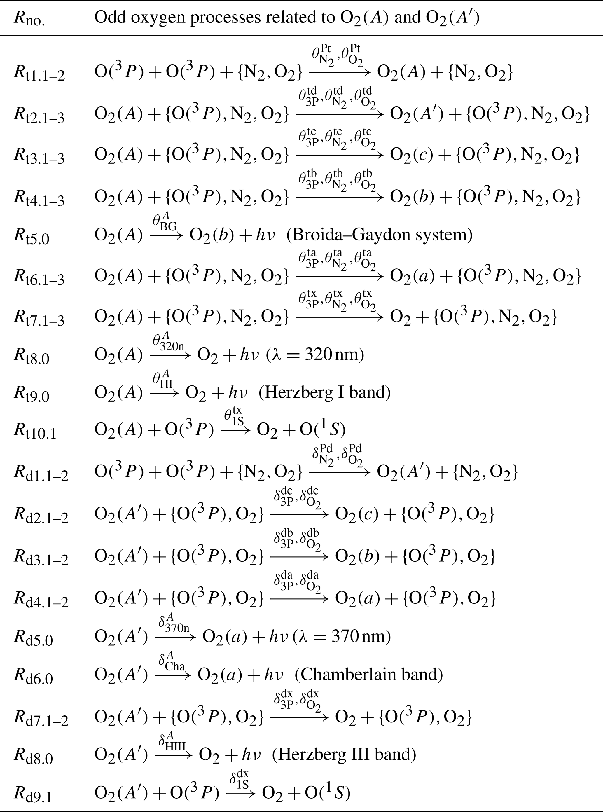
The C processes related to the Herzberg states and A′3Δu (hereafter referred to as ) are not considered in the G, M and H models. These C processes are related to the following:
-
the production of O2(A) (Rt1.1–2),
-
the de-excitation of O2(A) to (Rt2.1–3, Rt3.1–3, Rt4.1–3),
-
the Broida–Gaydon band emission (Rt5.0),
-
the de-excitation of O2(A) to O2(a, X) (Rt6.1–3, Rt7.1–3),
-
the Herzberg I band emission (Rt8.0, Rt9.0),
-
the O(1S) precursor responsible for the green line emission (Rt10.1, Rd9.1),
-
the production of O2(A′) (Rd1.1–2),
-
the de-excitation of O2(A′) to (Rd2.1–2, Rd3.1–2, Rd4.1–2),
-
the Chamberlain band emission (Rd5.0, Rd6.0),
-
the de-excitation of O2(A′) to O2(X) (Rd7.1–2) and
-
the Herzberg III band emission (Rd8.0).
These C processes and the corresponding reaction rates are provided in Tables 5 and 8, respectively.
The C processes related to the G, M and H processes complete the coupling of with each other and :
-
the photolysis of O2 and O3 (Rs1.(1,4–5), Rs2.(1–2,4–6)),
-
the singlet Herzberg state (Rc4.0, Rc5.1–2, Rc6.0, Rc7.2),
-
the atmospheric band emission (Rb2.1, Rb4.1,5–6),
-
the infrared atmospheric band emission (Ra2.1),
-
the red line emission (Rr2.2,4, Rr1.1–3, Rr3.0),
-
the green line emission (Rg1.3, Rg2.2) and
-
three-body recombination and ozone (Rx1.1–2, Rx2.1, Rx3.1–2).
These C processes are shown in Tables 6 and 7, and they were considered and discussed by Lednyts'kyy and von Savigny (2016). The corresponding reaction rates are shown in Tables 9, 10 and 11.
Table 6The processes shown here comprise the MAC model together with the processes shown in Table 5 and the processes shown in Table 7.
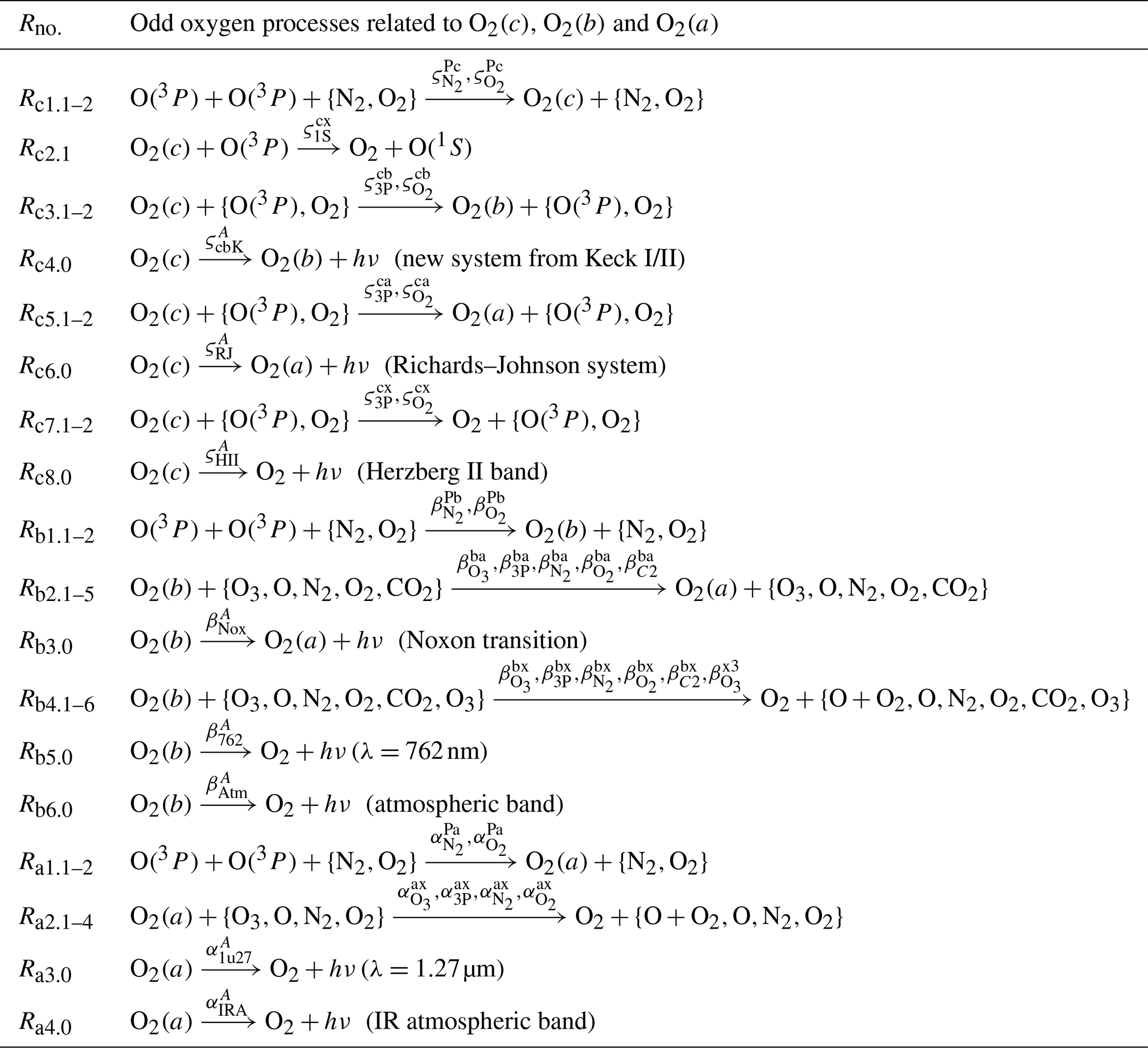
Table 7The processes shown here comprise the MAC model together with the processes shown in Tables 5 and 6.
Unknown or poorly constrained reaction rates of these complementary processes might be compromised by boundary effects if they were measured in the laboratory. Therefore, an appropriate photochemical model including many chemical species obtained on the basis of multiple emissions measured in situ in the Earth's atmosphere may be a valuable complement to laboratory experiments. In fact, unknown or poorly constrained reaction rates were tuned according to the verification and validation procedures discussed in Sect. 3.5 and applied on the basis of the ETON in situ measurements. The advantage of the ETON campaign compared to other rocket campaigns is that multiple emissions and [O(3P)] were measured almost simultaneously. This enables a comparison of the in situ and retrieved [O(3P)] using each particular emission profile described in Sect. 2.
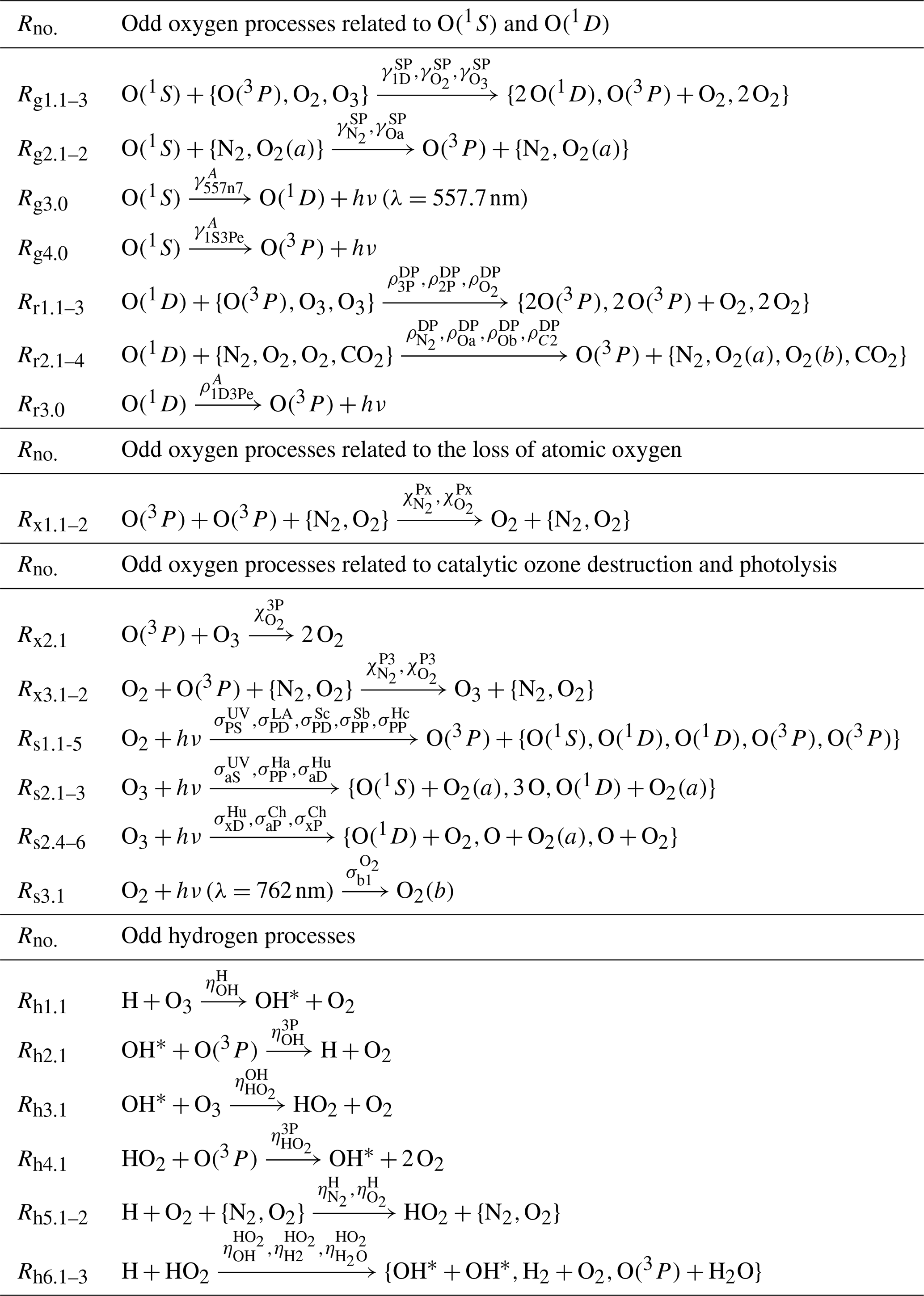
Figure 1 shows processes coupling and with each other, and Fig. 2 shows processes coupling and with each other.
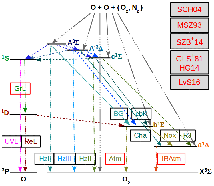
Figure 1O2 and O term diagrams showing processes of the MAC model comprised of processes considered in the G, M and H models and extended with complementary C processes. C processes are proposed to couple states of and with each other according to the hypothesis of Slanger et al. (2004b) (SCH04) stating that the Herzberg states are in constant collisional communication with the higher excited 5Π electronic state. All considered processes of the MAC model are provided in Tables 5, 6 and 7. Greer et al. (1981) (GLS+81) and Huang and George (2014) (HG14) considered the G processes, Mlynczak et al. (1993) (MSZ93) and Sharp et al. (2014) (SZB+14) the M processes, and Lednyts'kyy and von Savigny (2016) (LvS16) the C processes. Three-body recombination (association) reactions are indicated by the gray line shown by many dots and one long dash; they result in and due to reactions with the rate values βκ1 and ακ1, respectively, (McDade et al., 1986). Radiative losses and quenching processes are indicated by an abbreviation near the fine dashed line; see Table 1 for abbreviations. Radiative losses only are also indicated by an abbreviation. Quenching processes only are indicated by the dashed lines. The Herzberg states are all implemented as possible O(1S) precursors because their energy in various vibrational levels exceeds the 4.19 eV excitation energy difference with respect to the triplet O2(X) ground state.
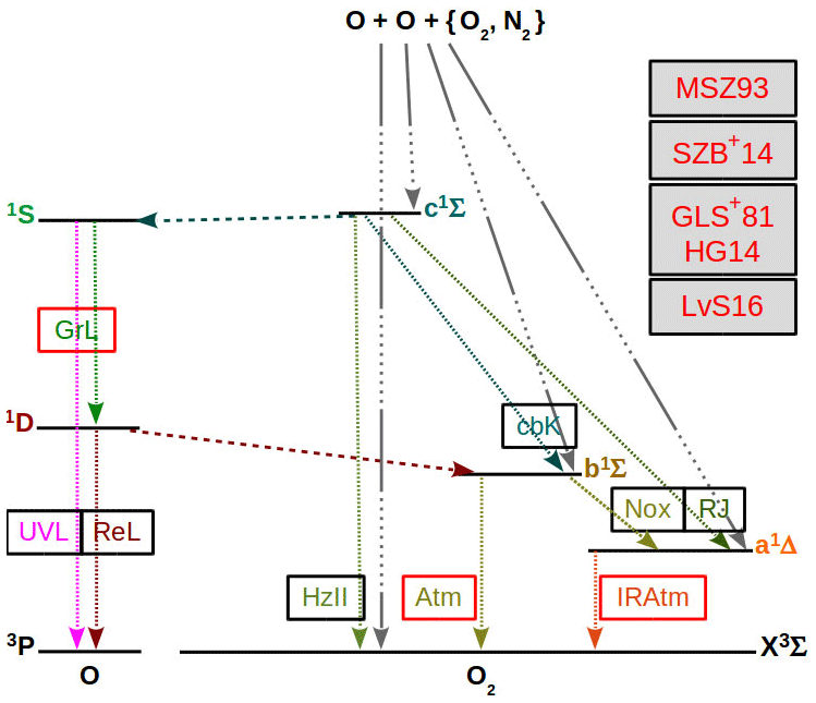
Figure 2Similar to Fig. 1, but for processes excluding the triplet O2(A) and O2(A′) Herzberg states from the MAC model. All considered processes of the MAC model indicated in the O2 and O term diagrams are provided in Tables 6 and 7. The following conclusions drawn by Slanger et al. (2004b) and Krasnopolsky (2011) help to interpret processes indicated here in the O2 and O term diagrams: (1) the and O2(X) () are triplet states, which are strongly coupled with each other; (2) transitions among the singlet states (, , a1Δg) and the triplet states are less probable because they require a spin flip; (3) the O2(c) and O2(b, a) states seem to be rather weakly coupled with each other, presumably because of Franck–Condon factors. This enabled the neglect of the states in the MAC model indicated in Fig. 2.
Considering the energy required for a spin flip in transitions among the triplet and singlet states it can be concluded that transitions from the states to the O2(X) state are more probable than spin forbidden transitions from the states to the states. Therefore, at least two versions of the MAC model can be implemented on the basis of the ETON measurements. The first one involves O2(A) and O2(A′), and the second one excludes them from the MAC model.
3.4 Tuning rate values of quenching processes implemented in the MAC model
All processes of the MAC model are provided in Sect. 3.3. These processes were separated into four groups: those considered in the G, M and H models as well as those considered complementary processes completing the MAC model and denoted as C processes. Unknown or poorly constrained reaction rate values of the C processes were tuned by comparing (1) retrieved and evaluated concentrations of excited chemical species, (2) in situ and evaluated VER profiles, and (3) in situ and retrieved [O(3P)] profiles. The validation procedure is related to the comparison of [O(3P)] profiles, and the verification procedure is related to the comparison of the other profiles; see Sect. 3.5. The verification and validation results support the use of the adjusted reaction rates provided in Tables 8, 9, 10 and 11.
Table 8Rate values of the processes considered in the MAC model involving O2(A) and O2(A′) and listed in Table 5. References: r01 – Smith and Robertson (2008), r02 – Bates (1988a), r03 – Lednyts'kyy and von Savigny (2016), r04 – Rodrigo et al. (1988), r05 – Bates (1988b), r06 – Krasnopolsky (2011), r07 – Kenner and Ogryzlo (1984), r08 – Stegman and Murtagh (1991), r09 – López-González et al. (1992a).

Table 9Rate values of the processes listed in Table 6. References: r10 – Predoi-Cross et al. (2008), r11 – Slanger (1978), r12 – Kenner and Ogryzlo (1983), r13 – Burkholder et al. (2015), r14 – Minaev and Ågren (1997). The labels r01, r02, r03, r06 and r08 were used in Table 8. The enthalpy change (ΔH) was determined at standard temperature and pressure; see Table 11 for abbreviations.
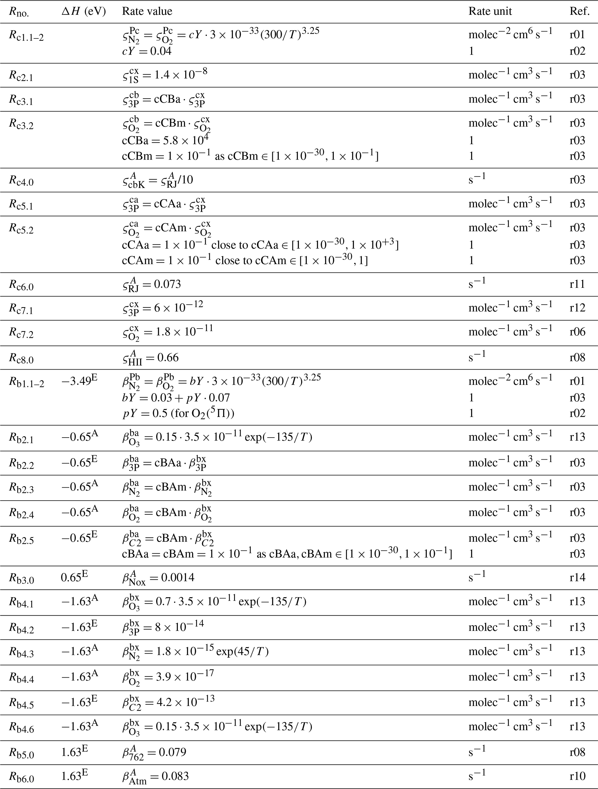
Table 10Rate values of the processes listed in Tables 6 and 7. References: r15 – Pendleton et al. (1996), r16 – Krauss and Neumann (1975), r17 – Capetanakis et al. (1993), r18 – Gordiets et al. (1995), r19 – Atkinson and Welge (1972), r20 – Kenner and Ogryzlo (1982), r21 – Kramida et al. (2015), r22 – Pinheiro et al. (1998), r23 – Sakai et al. (2014). The labels r01, r02 and r03 were used in Table 8, and the labels r13 and r14 were used in Table 9. The enthalpy change (ΔH) was determined at standard temperature and pressure; see Table 11 for abbreviations.

Table 11Rate values of the processes listed in Table 7. References: r24 – Nicolet (1971), r25 – Nicolet et al. (1989), r26 – Nicolet and Kennes (1988), r27 – Nicolet (1989), r28 – Mlynczak et al. (1993), r29 – Atkinson et al. (1997), r30 – Khomich et al. (2008). The labels r01, r02 and r03 were used in Table 8, and the label r13 was used in Table 9. The exothermic reaction energy content was determined for each reaction at standard temperature and pressure; see the ΔH column for the enthalpy change. ΔH values were read out (unit: eV) from Roble (2013) (marked by character R) and (units: kJ mol−1) from Atkinson et al. (1997) (marked by character A). Additionally, ΔH values were evaluated (marked by character E).

As mentioned in Sect. 2, unknown or poorly constrained reactions in the MAC model were tuned on the basis of the ETON in situ measurements and applied to data sets measured during the WADIS-2, WAVE2000 and WAVE2004 campaigns; see Lednyts'kyy et al. (2019) for details. Dr. Fytterer and Dr. Sinnhuber from the Karlsruhe Institute of Technology suggested the rate values of the reactions Rb2.1, Rb4.1, Rb6.0, Rr1.2 and Rr2.3 for the data sets of the WAVE2004 campaign. The other reaction rates were adjusted on the basis of the described verification and validation procedures. Particularly, the Ra2.2 reaction rate was also adjusted within the range provided by Burkholder et al. (2015), who gave the upper limit of this reaction. Rate values of the reactions Rt10.1, Rd9.1 and Rc2.1 regarding O(1S) production were adjusted by taking the studies of Krasnopolsky (2011), Huang and George (2014), Steadman and Thrush (1994), and Torr et al. (1985) into account. The adjustment of the rate values of the three-body recombination reactions is described in Sect. 4.1.
The tuning of the rate coefficients was carried out by changing the values of dimensionless scaling factors (cTDu, cTCu, cTBu, cTAu, cDCu, cDBu, cDAu, cCBa, cCBm, cCAa, cCAm, cBAa, cBAm and cAXa shown in Tables 8, 9, 10 and 11), which are multiplied with the corresponding rate coefficients and describe the strength of the coupling among O2 states as follows:
-
cTDu is for coupling of O2(A) and O2(A′), cTCu – O2(A) and O2(c), cTBu – O2(A) and O2(b), cTAu – O2(A) and O2(a).
-
cDCu is for coupling of O2(A′) and O2(c), cDBu – O2(A′) and O2(b), cDAu – O2(A′) and O2(a).
-
cCBa is for coupling of O2(c) and O2(b) by quenching of O2(c) with O(3P), cCBm – O2(c) and O2(b) by quenching of O2(c) with O2(X), cCAa – O2(c) and O2(a) by quenching of O2(c) with O(3P), cCAm – O2(c) and O2(a) by quenching of O2(c) with O2(X).
-
cBAa is for coupling of O2(b) and O2(a) by quenching of O2(a) with O(3P), cBAm – O2(b) and O2(a) by quenching of O2(b) with O2(X).
-
cAXa is for coupling of O2(a) and O2(X) by quenching of O2(a) with O(3P).
The values of these scaling factors were altered to determine their influence on [Ocurrent] calculating differences with respect to [Oreference] retrieved without adjusting these scaling factors. The differences were calculated according to Eq. (5) and used in the sensitivity analysis; see the third column of Tables 8, 9, 10 and 11 for a summary. For instance, perturbations in cTDu values do not cause changes in retrieved and evaluated MAC output parameters. Therefore, the tested interval is shown as in Table 8, and cTDu is set to an arbitrary value of .
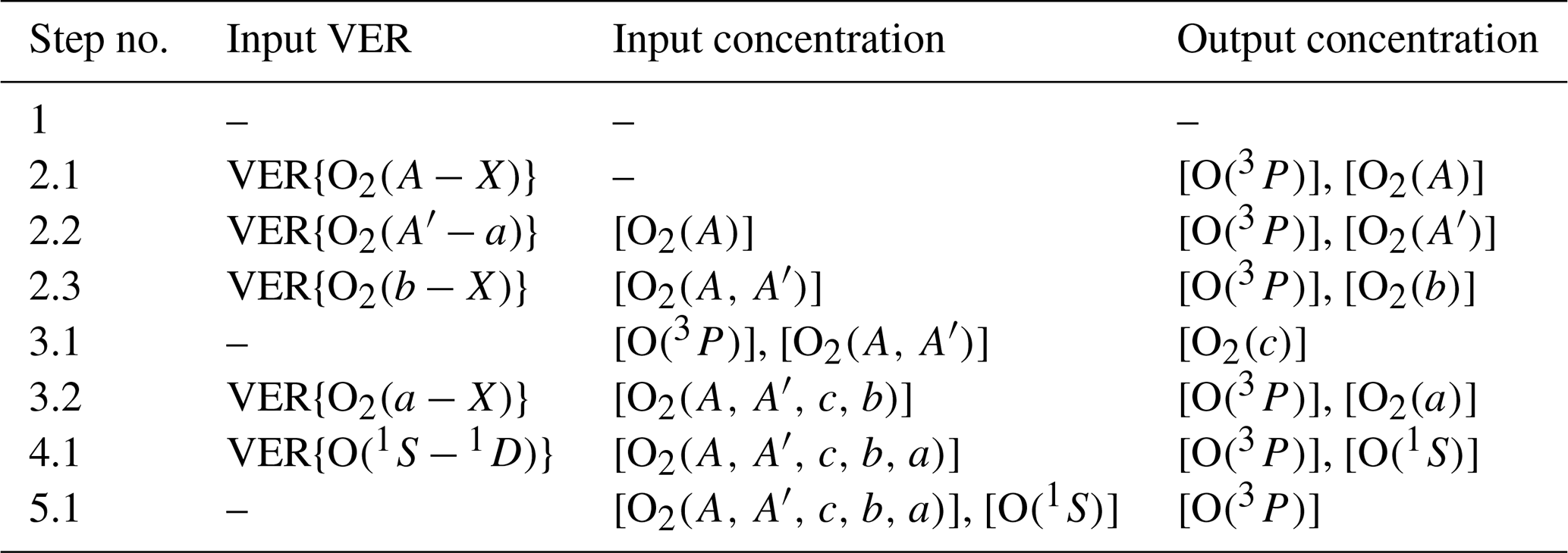
Table 12Overview of the calculation steps carried out using the MAC model. The first column shows the step number. The input concentrations shown in the third column were retrieved at one of the previous steps and are required together with profiles of input VER and the other MAC input parameters at the current retrieval step. The other MAC input parameters should be at least comprised of temperature (T), O2 and N2 that can be simulated using the NRLMSISE-00 model. If only these MAC input parameters are available, then the prior step 1 described in Sect. A1 is omitted. Nevertheless, if [O3] and [H] were also available among the other MAC input parameters, then [O(1S)], [O(1D)], [OH∗] and [HO2] would be calculated at the prior step 1 and also used as MAC input parameters at the following steps.
Additionally, the rate value of the Ra2.2 reaction was adjusted in the interval of possible values multiplied by molec−1 cm3 s−1 and applied at step 3.2 shown in Table 12. This adjustment of the scaling factor cAXa is allowed because molec−1 cm3 s−1 is given by Burkholder et al. (2015) as the upper interval value. A Ra2.2 reaction rate of higher than molec−1 cm3 s−1 seems by sight to cause higher [O(3P)] peak values than those obtained with molec−1 cm3 s−1. Therefore, is used so that the Ra2.2 reaction rate equal to molec−1 cm3 s−1 is employed in the MAC model.
3.5 Verification and validation of calculations carried out with the MAC model
The input parameters of the MAC model are described in Sect. 2 and include VER profiles retrieved on the basis of in situ measurements during the ETON rocket campaign (Greer et al., 1986) as well as profiles of temperature (T), [N2] and [O2] obtained using the semi-empirical model NRLMSISE-00. Among the mentioned VER profiles are VER{O2(A−X)} (Herzberg I band, HzI), VER (Chamberlain band, Cha), VER{O2(b−X)} (atmospheric band, Atm), VER{O2(a−X)} (infrared atmospheric band, IRAtm) and VER{O(1S−1D)} (green line, GrL). These VER profiles were retrieved on the basis of the raw integrated data (Greer et al., 1986) marked by character R, e.g., R-VER{O2(A−X)}.
The concentrations of various chemical species were retrieved using sequentially applied continuity equations in the steady state, i.e., polynomial equations of the second or the third order. An overview of all retrieval steps of the MAC model is provided in Appendix A devoted to the description of all algorithmic steps; see also Table 12 for a short overview. The input VER profiles shown in Table 12 correspond to O2 transitions shown in Table 1. In fact, all reactions relevant for the particular chemical species were used in the retrievals, and the retrieved concentration profiles are marked by character R, e.g., R-[O2(A)]. Additionally, concentrations of the same chemical species were evaluated by dividing the R-VER profiles, which correspond to the particular chemical species, by the respective transition probability. The evaluated concentration profiles are marked by character E, e.g., E-[O2(A)]. As for the evaluated VER profiles, which are marked by character E as E-VER profiles (e.g., E-VER{O2(A−X)}), they are obtained by multiplying the retrieved concentrations of the same chemical species by the respective transition probability.
The results of calculations carried out using the MAC model are verified by a visual comparison of retrieved and evaluated profiles, i.e., the respective emission and concentration values. Note that the prior step 1 shown in Table 12 and briefly described in Sect. A1 is omitted for the ETON campaign because such input parameters as [O3] and [H] are not known a priori. Instead, the short list of the input parameters required to run the MAC model is applied: T, [N2], [O2] from the NRLMSISE-00 model and VER profiles from the ETON campaign. For instance, the quadratic continuity equation is solved to retrieve R-[O2(A)] on the basis of R-VER{O2(A−X)} using all relevant processes of the MAC model. This retrieval step is shown as step 2.1 in Table 12 and step 2.1 described in Sect. A2.1 in Appendix A. Then, the verification of calculations at step 2.1 is carried out by comparing R-VER{O2(A−X)} with E-VER{O2(A−X)} and R-[O2(A)] with E-[O2(A)]. The cubic equation is solved at step 2.2 on the basis of T, [N2], [O2], R-VER and R-[O2(A)]. Then, the verification of calculations at step 2.2 is carried out by comparing R-VER with E-VER and R-[O2(A′)] with E-[O2(A′)].
Note that values of the in situ R-VER{O(1S−1D)} profile are less than zero randomly below 92 km due to the measurement noise. Therefore, the in situ R-VER{O(1S−1D)} profile is approximated by the asymmetrical Gaussian distribution described by Semenov (1997) and Khomich et al. (2008) to obtain the shown A-VER{O(1S−1D)} profile and to retrieve the corresponding [O(1S)] profile.
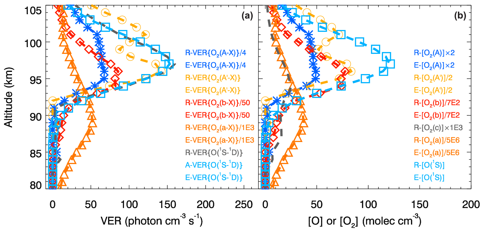
Figure 3The retrieved VER (R-VER) profiles obtained during the ETON campaign (see Sect. 2) and the evaluated VER (E-VER) profiles obtained using the MAC model involving O2(A) and O2(A′) are shown in panel (a) by the dashed lines and symbols. Calculations carried out using the MAC model involving O2(A) and O2(A′) are verified visually by comparing the R-VER and E-VER profiles. Concentrations of various chemical species were retrieved on the basis of the corresponding R-VER profiles and all relevant processes of the MAC model; these concentrations are marked with a character R and shown in panel (b) by the dashed lines. The respective transition probabilities are only used to evaluate concentrations marked with a character E as well as E-VER profiles. Again, the evaluated concentrations are shown with the use of symbols as done for E-VER profiles. Two corresponding profiles (R-VER and E-VER as well as the retrieved and evaluated concentrations) seem to be in perfect agreement with each other by sight. This implies that all calculations carried out with the MAC model are consistent with each other and the results are coherent with measurements. The corresponding consistency tests are described in Sect. A2.4, A3.3 and A4.2. Note that the conversion between profile values of VER and concentrations is based on trivial but required calculations provided in Sect. A2.1, A2.2, A2.3, A3.2 and A4.1. The abbreviations indicating emissions are explained in Table 1, and the sequence of the retrieval steps is provided in Table 12. Values of temperature, [N2] and [O2] were obtained by using the NRLMSISE-00 model (see Sect. 2) for the time and place of the P229H rocket.
The retrieved and evaluated VER profiles indicated by the dashed lines and the symbols, respectively, shown in Fig. 3a are compared with each other by sight to verify calculations carried out with the MAC model involving O2(A) and O2(A′). The retrieved and evaluated VER profiles belonging to each pair regarding the considered excited O2 state seem to be in perfect agreement with each other by sight. Next, the retrieved and evaluated concentration profiles shown in Fig. 3b by the dashed lines and the symbols, respectively, are also compared with each other for each retrieval step. These profiles also seem to be in perfect agreement with each other by sight. The excellent agreement of the retrieved and evaluated products (VER or concentration profile) enables the conclusion that all calculations carried out using the MAC model are consistent with each other and coherent with measurements.
Before we discuss results of the [O(3P)] retrievals obtained with the proposed MAC model, a short overview of the previously used photochemical models is given to estimate our current situation and to argue whether the proposed MAC model is needed. The published photochemical models based on the processes provided in Table 2 resulted in the following continuity equations discussed here with respect to [O(3P)]:
-
the well-known quadratic equation of McDade et al. (1986) (MMG+86) was applied to the atmospheric band emissions at 762.2 nm (see Sects. 1 and 3.1),
-
the well-known cubic equation (2) was applied to the green line emissions at 557.7 nm (see Sect. 3.1) and
-
the extended cubic equation proposed by Gobbi et al. (1992) (see Eq. 3), was applied to the green line emission at 557.7 nm with the empirical coefficients of Lednyts'kyy et al. (2015) (LSE+15) and solved using the analytical method of Semenov (1997) modified by Lednyts'kyy et al. (2015).
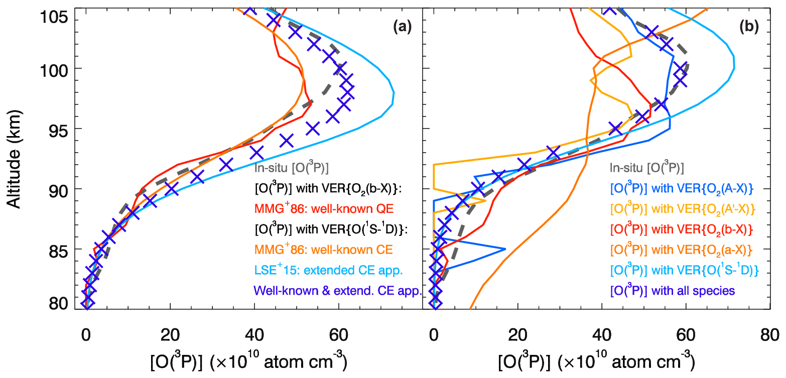
Figure 4The in situ and retrieved [O(3P)] profiles are shown and compared with each other. The in situ [O(3P)] profile obtained during the ETON campaign (see Sect. 2) is shown by the dashed gray line to validate [O(3P)] retrievals. The well-known quadratic equation (QE) and the well-known cubic equation (CE) of McDade et al. (1986) (MMG+86) as well as the extended CE of Lednyts'kyy et al. (2015) (LSE+15) were applied to retrieve the [O(3P)] profiles shown in panel (a). [O(3P)] profiles retrieved according to the cubic equations seem to represent two profiles of extreme values with respect to the in situ [O(3P)] profile. Therefore, they were arithmetically averaged (see the violet crosses in panel a of this figure) and seem to be in good agreement with the in situ [O(3P)] profile values. This was done to estimate the efficiency of the known photochemical models, but we do not ascribe any deeper significance to this finding. Empirical coefficients were introduced in both cubic equations phenomenologically, which stimulated the proposal of the MAC model. The MAC model involving O2(A) and O2(A′) (see Sect. 3.3) was applied at the retrieval steps provided in Table 12 and consequently applied to retrieve the [O(3P)] profiles shown in panel (b) by the solid colored lines similar to Fig. 3. Although steps 2.1, 2.2, 2.3 and 3.2 applied on the basis of some ETON VER profiles result in lower [O(3P)] values compared to the in situ ones, the [O(3P)] retrieval carried out at step 4.1 on the basis of VER{O(1S−1D)} results in higher values. The last retrieval step 5.1 applied on the basis of the concentrations of all chemical species retrieved at the previous steps results in [O(3P)] values being in good agreement with the in situ values.
These three continuity equations are applied, and the retrieved [O(3P)] profiles are shown in Fig. 4a. The peak [O(3P)] profile values retrieved according to the well-known quadratic and cubic equations are lower, but those of the extended cubic equation are higher than the peak values of the in situ ETON [O(3P)] profile. The [O(3P)] profile values retrieved according to the well-known and extended cubic equations can be considered two profiles of extreme values because the in situ [O(3P)] profile values seem to be equidistant with respect to the retrieved ones. One could assume that arithmetical averaging of the extreme [O(3P)] profile values might be appropriate to finalize the retrievals, resulting in [O(3P)] profile values denoted by the violet crosses shown in both figures. Indeed, the averaged peak [O(3P)] profile values are almost equal to those of the in situ [O(3P)] profile. However, now we do not see any deeper significance in this finding. Empirical coefficients were derived for these previously used photochemical models phenomenologically, i.e., in relation to reaction rates in which an unidentified is involved. Therefore, [O(3P)] retrievals on a new photochemical basis are required. Note that processes of the previously used photochemical models were also used to propose the MAC model, which is applied as follows.
[O(3P)] profiles retrieved using the MAC model involving O2(A) and O2(A′) are shown in Fig. 4b. The in situ [O(3P)] profile is compared with the [O(3P)] profiles obtained at the retrieval steps provided in Table 12. The retrieved profiles are indicated in the same color used to show them in the legend. The peak values of the [O(3P)] profiles retrieved directly on the basis of VER{O2(A−X)}, VER, VER{O2(b−X)} and VER{O2(a−X)} are lower than those of the in situ ETON [O(3P)] profile, but the peak values of the [O(3P)] profile retrieved at step 4.1 on the basis of VER{O(1S−1D)} are higher. The peak magnitude and altitude values as well as the shape of the [O(3P)] profile retrieved at the last step 5.1 on the basis of all chemical species are approximately the same compared to those of the in situ ETON [O(3P)] profile.
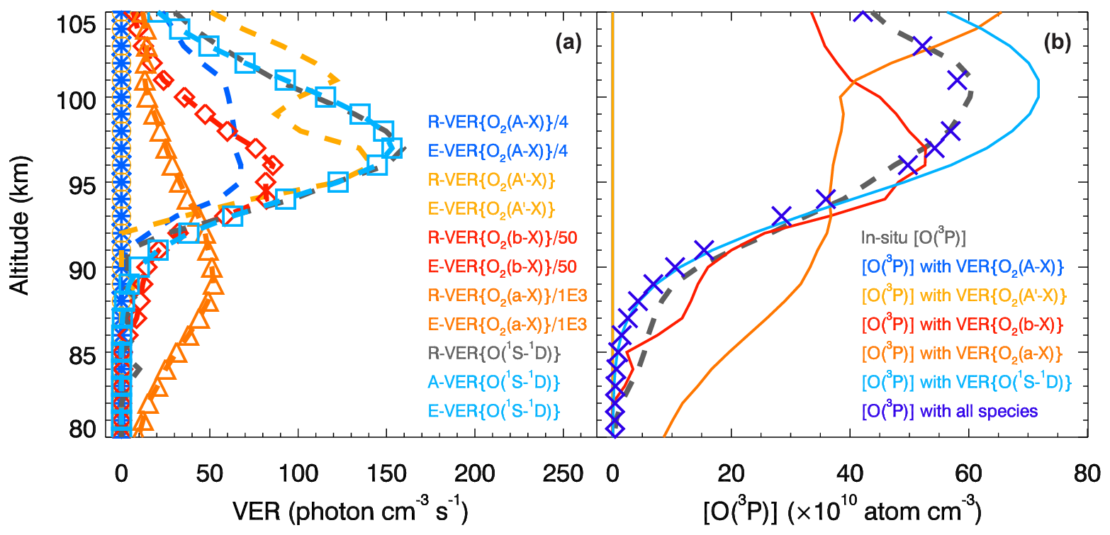
Figure 5Similar to Figs. 3 and 4, but showing results obtained with the MAC model excluding O2(A) and O2(A′). The first two retrieval steps 2.1 and 2.2 are not carried out, because now the VER{O2(A−X)} and VER profiles are not considered in the MAC calculations. The in situ and retrieved VER and [O(3P)] profiles obtained at steps 2.3, 3.2, 4.1 and 5.1 agree with each other by sight and with those shown in Fig. 4, and the MAC calculations are concluded to be verified and validated. The comparison of products related to VER{O(1S−1D)} indicated by the cyan color and shown in this figure as well as in Fig. 3 enables the conclusion that the contribution of O2(A) and O2(A′) to the O(1S) production is negligible. Therefore, O2(c) can be considered the major O(1S) precursor. It follows also that the triplet Herzberg states (, A′3Δu) are more strongly coupled with the triplet ground state () than with the singlet states (, , a1Δg) because the O2(X) production is considered to be invariable.
In the following, the retrieval results obtained with the MAC model excluding O2(A) and O2(A′) are shown in Fig. 5 and discussed in comparison to those obtained with the MAC model involving O2(A) and O2(A′) shown in Figs. 3 and 4.
Profiles of VER and [O(3P)] obtained at steps 2.3, 3.1, 3.2, 4.1 and 5.1 are shown in Fig. 5. In fact, values of E-VER{O2(A−X)}, E-VER, R-[O2(A)] and R-[O2(A′)] are equal to zero, whereas E-[O2(A)] and E-[O2(A′)] cannot be shown in Fig. 5 because of the division by transition probabilities set to zero at steps 2.1 and 2.2.
Values of VER profiles were compared with each other for two cases: (1) using the MAC model involving O2(A) and O2(A′) (see Fig. 3a) and (2) using the MAC model excluding O2(A) and O2(A′) (see Fig. 5a). This comparison enables the conclusion that the calculations carried out are consistent with each other, leading to results coherent with measurements in both cases. Because R-VER{O(1S−1D)} and E-VER{O(1S−1D)} shown in these figures seem to be in perfect agreement with each other, we can argue about the O(1S) production implemented via different pathways indicated in Figs. 1 and 2. In fact, our suggestions about the origin of the O(1S−1D) green line emission are also backed up by the comparison of various [O(3P)] shown in Figs. 4b and 5b. Specifically, O2(c) can be considered the major O(1S) precursor because the contribution of processes involving O2(A) and O2(A′) to the O(1S) production is negligible.
The [O(3P)] profile values retrieved at step 3.2 on the basis of VER{O2(a−X)} (infrared atmospheric band, IRAtm) are variable with a variability higher than those of the in situ ETON [O(3P)] profile at altitudes higher than 102 km and lower than 95 km; see Figs. 4 and 5. [O(3P)] profile values retrieved at step 3.2 do not agree with the in situ ETON [O(3P)] profile values to the same degree as the [O(3P)] profile values retrieved at the other steps. Llewellyn and Solheim (1978) analyzed emissions in the IRAtm and Meinel bands and proposed the rate of the reaction , which they suggested to implement in a photochemical model to retrieve [O(3P)]. The reaction Rh2.1 implemented in the MAC model and shown in Table 7 is similar to that considered by Llewellyn and Solheim (1978): , where OH∗ describes the hydroxyl radical in all possible levels ν′. It should be mentioned that it would be possible to retrieve [O(3P)] if the vibrational population of OH(ν′) were known. Wayne (1994) presented an excellent overview of reactions involving O2(a) and assumed that the reaction emphasized by Llewellyn and Solheim (1978) only produces about one-half of the VER{O2(a−X)} intensity needed. Wayne (1994) suggested that the reaction can be neglected due to its negligible contribution, which was experimentally confirmed. Hislop and Wayne (1977) emphasized two sources of the emission line at λ1270=1270 nm. The first source is the transition at λ1270 that enables the determination of VER{O2(a−X)} profiles. The second source is the electronic transition at nm, which is very close to λ1270. 2A′′ denotes the ground state of HO2, 2A′ its first excited state, and the three numbers in parentheses the various levels of the vibrational excitation. Additionally, Hislop and Wayne (1977) mentioned the reaction , which negligibly produces O2(a). It is possible to process OH∗ emissions in future versions of the MAC model applied to measurements obtained during the ETON campaign, but emissions related to the excited HO2 () were measured neither during the ETON campaign nor other rocket campaigns known to the authors of this article. Unfortunately, it would not be enough to extend future versions of the MAC model with processes considering vibrational levels of OH∗ because of the contribution.
Sharma et al. (2015) proposed a new mechanism responsible for the deactivation of OH∗ as follows: . Sharma et al. (2015) emphasized that this mechanism is represented by two reactions producing a transient complex at first, which is de-excited, resulting in the products shown in the proposed mechanism on the right. Contributions of processes involving both OH∗ and HO2 to the production of O2(a) need to be considered in order to retrieve [O(3P)] using VER{O2(a−X)}. This enables the conclusion that the disagreement of the reference [O(3P)] profiles with the current [O(3P)] profiles retrieved at step 3.2 using the MAC model will remain if only the currently known in situ measurements are applied.
In summary, the MAC model was carefully applied to retrieve [O(3P)] on the basis of a limited number of VER profiles: (1) including or neglecting VER{O2(A−X)} and VER profiles and (2) using all VER profiles or a VER{O2(b−X)} profile only. This is possible because calculations carried out using the MAC model are separated by steps, and the concentrations of various O2 states are considered at each of the retrieval steps listed in Table 12.
3.6 Influence of perturbations in model parameters on [O(3P)] retrieved using the MAC model
The results of the [O(3P)] retrievals carried out with the MAC model depend on the values of the following MAC input parameters: temperature (T), [N2], [O2] and VER profiles. Therefore, the impact of perturbations in VER profiles by the error values provided by Greer et al. (1986) (see Sect. 2) and the impact of perturbations in profiles of T, [N2] and [O2] by 5 % of their values on the retrieved [O(3P)] profiles are estimated and discussed in this section. Specifically, these retrieved (hereafter referred to as perturbed) [O(3P)] profiles are compared with the unperturbed (hereafter referred to as reference) [O(3P)] profiles by estimating differences between them as follows:
where the [Oreference] profiles are shown in Fig. 4. To keep the results obtained according to Eq. (5) positive, perturbations in T were chosen to be +5 % of T, but perturbations in [N2] and [O2] by −5 % of the respective ([N2]+[O2]) values. Perturbations in VER profiles were introduced by positive values of the respective error values. Specifically, the absolute accuracy of VER{O2(a−X)} (infrared atmospheric band, IRAtm) values was assumed to be ±20 %, and the absolute accuracy of the other VER values was assumed to be ±10 % according to Greer et al. (1986); see Sect. 2 for details.
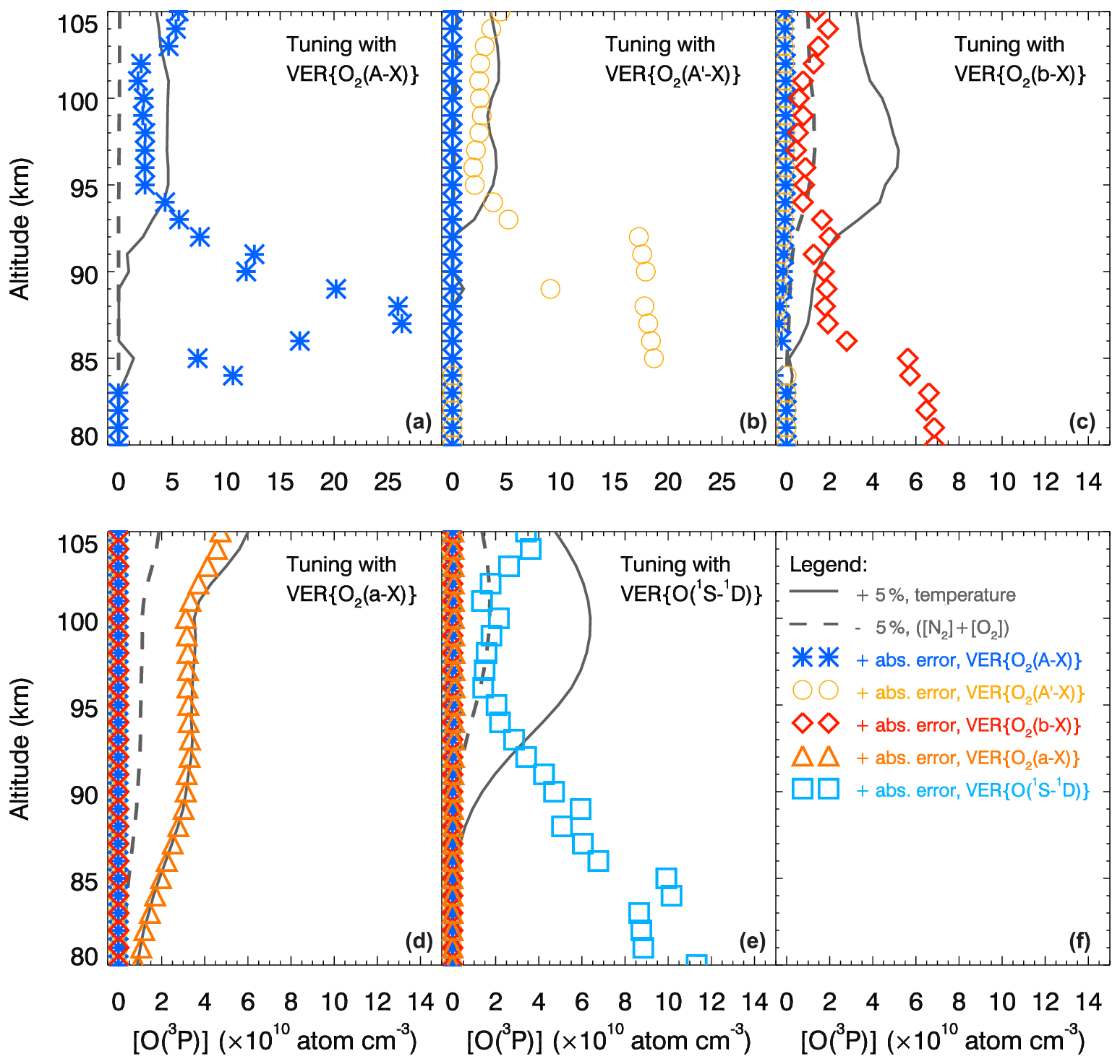
Figure 6Effects of perturbations in the MAC input parameters on the retrieved [O(3P)] profiles. The retrievals were performed at steps 2.1, 2.2, 2.3, 3.2 and 4.1 described in Table 12 on the basis of the following perturbed input parameters: volume emission rates (VERs), temperature (T), [N2] and [O2]. Additionally, [O(3P)] profiles were retrieved on the basis of the unperturbed input parameters and denoted as reference [O(3P)] profiles shown in Fig. 4. Finally, differences between the reference and perturbed [O(3P)] profiles were estimated and are shown in five panels using the colors of the perturbed input parameters in the legend, which is shown in panel (f). The units of the differences shown in panels (a)–(c) are the same as those of panels (d)–(f). VER values were perturbed by values of the absolute error: +20 % for the VER{O2(a−X)} profile and +10 % for the other VER profiles. Data sets of T, [N2] and [O2] were obtained using the NRLMSISE-00 model and perturbed by 5 %: +5 % for the T values and −5 % for the sum of the [N2] and [O2] values. Profiles of [O(3P)] differences determined by perturbing VER profiles are shown by colored symbols, those determined by perturbing T profiles by solid gray lines, and those determined by perturbing ([N2]+[O2]) profiles by dashed gray lines. Each retrieval step is indicated by the name of the corresponding in situ ETON VER profile shown in the upper right corner of each panel.
Both the perturbed and reference [O(3P)] profiles were retrieved using the MAC model with one MAC input parameter perturbed at a time according to the description provided at the beginning of this section. For instance, values of one VER profile only were perturbed at the particular retrieval step; see Table 12 for an overview of all steps of the consequent retrieval procedure. Figure 6 shows ϵ values (units: atoms cm−3), illustrating the influence of the perturbed input parameters on [O(3P)] profiles. Because the number of VER profiles used in the [O(3P)] retrieval increases with each step, the number of profiles of [O(3P)] differences also increases from panel (a) to panel (e) of this figure. Note that a VER profile, which was considered to have a significant impact at one of the retrieval steps performed previously to calculate the corresponding concentration profile, was taken only implicitly into account at the current retrieval step, at which these concentrations are considered instead of the corresponding VER profile. A comparison of difference values shown in various panels indicates that perturbations in the VER and T profiles introduced simultaneously will cause the highest impact on [O(3P)] profiles.
In situ measurements obtained during the ETON campaign enable the estimation of the efficiency of [O(3P)] retrievals carried out using the well-known photochemical models and the proposed MAC model; see Sect. 3.5. For instance, Lednyts'kyy et al. (2015) considered as the O(1S) precursor to retrieve the SCIAMACHY [O(3P)] time series; see Sect. 3.1 and 3.5. Further work discussed here and by Lednyts'kyy and von Savigny (2016) and Lednyts'kyy et al. (2018) validated the suggestions and retrievals of Lednyts'kyy et al. (2015) carried out on the basis of various rocket campaigns that enabled the proposal of the MAC model. For instance, the states O2(c b a, X) were adopted in the MAC model from the M and H models (see Sect. 3.2.1 and 3.2.2, respectively) instead of considered by Lednyts'kyy et al. (2015) in the G model (see Sect. 3.1).
Additionally to the excited singlet states , Huestis (2002) and Slanger et al. (2004b) considered O2(5Π) and the triplet Herzberg states (O2(A) and O2(A′)) coupled with . Specifically, processes coupling and with each other were proposed as complementary processes in the MAC model.
The removal of the O2(5Π)– group and the weak coupling of the triplet states with the singlet states enabled the omission of the states in the MAC model. There are three reasons for the weak coupling of the triplet states with the singlet states. Firstly, the O2(A) and O2(A′) states are strongly coupled with each other because the vibrational states of these triplet states are energetically very close to each other. Vibronic energy levels of are shown in Fig. 8 by Goodman and Brus (1977). The atlas of terrestrial nightglow emission lines in the range 314–1043 nm, including the emission lines of these O2 states, is provided in Table 3 as a compressed form of the electronic supplement of Cosby et al. (2006). Vibrational states of these triplet states and the O2(c) singlet state are also very close to each other, but the spin flip energy is required for transitions from these triplet states to the O2(c) singlet state. Secondly, the probability of transitions from to O2(b, a) is supposed to be negligibly higher than that of transitions to O2(X) because of Franck–Condon factors. Considering Franck–Condon factors and the corresponding internuclear distances (INDs), it should be emphasized that the difference in INDs between the excited O2(A) state and the ground O2(X) state is approximately equal to the difference in INDs between the excited O2(A′) state and the ground O2(X) state. Additionally, the difference in INDs between the excited O2(b) state and the ground O2(X) state is approximately equal to the difference in INDs between the excited O2(a) state and the ground O2(X) state. Thirdly, the probability of transitions from to O2(X) is supposed to be significantly higher than that of transitions to O2(b, a) because of a required spin flip. Note that data about INDs and Franck–Condon factors are used to calculate the transition intensities (Hollas, 2004). Therefore, we conclude that transitions from to O2(X) are more probable than transitions from to .
It should be kept in mind during the interpretation of the obtained results that the uncertainties of the ETON data sets are 10–20 % in VER peak values; see Sect. 2. Varying the MAC input data within these uncertainty ranges significantly influences the magnitude of products obtained with the MAC model. For example, the retrieved [O(3P)] peak values increase by up to 40 % if VER values are increased by 10 % due to the VER uncertainty; compare Figs. 6 and 3. Additionally, uncertainty in the in situ [O(3P)] profile values of less than about 40 % in [O(3P)] peak values is very high, implying that novel in situ data sets obtained with more accurate measurement techniques should be measured in the future. In fact, the ETON in situ measurements were used to tune unknown or poorly constrained rate values of the complementary processes, and the importance of precise in situ measurements is tremendous. Nevertheless, rate values of the processes implemented in the MAC model are considered to be validated through a comparison of the in situ and retrieved [O(3P)] profiles. In the following three sections we discuss the tuning based on the ETON data set.
4.1 Discussion of the obtained results regarding tuned rate values for implemented three-body recombination processes
The MAC model was proposed on the basis of the hypothesis of Huestis (2002) and Slanger et al. (2004b), who stressed that association rates of excited O2 states in the three-body recombinations must be modified because O2 molecules in various excited states collide with each other and other molecules so that an excitation transfer takes place. However, Huestis (2002) and Slanger et al. (2004b) did not provide modified association rates. This was also emphasized by Krasnopolsky (2011), who applied the two-step Barth excitation transfer scheme for each of the ETON VER profiles separately. Thus, Krasnopolsky (2011) substantially limited (compared to Krasnopolsky, 1986) the number of considered chemical reactions related to O2(5Π). Because the lifetime of O2(5Π) is less than ∼0.4 µs (Slanger and Copeland, 2003), it is impossible to determine a number of reaction rates involving O2(5Π) in the laboratory. For this reason reactions involving O2(5Π) cannot be adequately included in chemical–dynamic time-dependent atmospheric models. Nevertheless, the association rate values of O2 states were tuned with the use of the hypothesis of Slanger et al. (2004b) to apply them in the MAC model as follows. Firstly, the theoretically known association rates (Bates, 1988a) were considered. Then, they were used to obtain the new association rate values of ; see the respective yielding factors bY, aY and xY in Tables 9 and 10. Specifically, values of the known association rates were increased using the association rate (pY) of O2(5Π). For instance, the association rate of O2(b) was increased by an arbitrary value of 7 % of the pY value to determine a new value of bY. In a similar way, the association rates of O2(a) and O2(X) were increased by arbitrary values of 68 % and 25 % of the pY value to determine new values of aY and xY, respectively.
It should be noted that Bates (1988a) provided the association rates for by applying the concept of a hard sphere to the reaction rates in the three-body recombinations () as was done by Bates (1951), Wraight (1982) and Smith (1984). It is remarkable that N2 was used as the third body in laboratory studies and that the reaction rate of the three-body recombination updated by Smith and Robertson (2008) is lower than that one provided by Campbell and Gray (1973) above 200 K and higher below 200 K. Nevertheless, Campbell and Gray (1973) and Smith and Robertson (2008) assumed the obtained reaction rate () to be equal to the one () considering O2 to be the third body because of the hard-sphere concept used. Unfortunately, neither nor is provided in the established studies on chemical kinetics, e.g., the Jet Propulsion Laboratory databases (Burkholder et al., 2015). It is worth mentioning that Bates (1979) interpreted the Chapman excitation process as follows: two colliding O(3P) atoms create an electronically excited O2 molecule, which is presumably in the upper Herzberg state (Greer et al., 1987); see Sect. 1 for details. This altogether implies that an interaction of O2 in the ground or excited states with one or more O(3P) atoms is a complicated process worthy of further investigation, and the hard-sphere concept should be used with caution.
There are two main adjustments done in the MAC model with respect to the three-body recombinations. The first one is related to the increased association rates of taking collisions of higher excited O2 molecules with O2(5Π) into account and being implicitly considered in the MAC model. The second one is related to the increase in compared to of the reactions Rx1.2 and Rx1.1, respectively. This adjustment was done because the hard-sphere concept used is probably misleading and because other O(3P) loss processes were required to be implicitly implemented in the MAC model according to the verification and validation procedures. The origin of the required O(3P) loss processes is currently not definitely known because both photochemical and dynamical phenomena might contribute to the total O(3P) loss. Note that the O2 photodissociation into O(3P) atoms has its maximum at ∼120 km according to Solomon and Qian (2005), and Colegrove et al. (1965) invoked eddy diffusion to describe the O(3P) loss by transport from the lower thermosphere downwards.
Two cases are considered in terms of adjusting the rate values of the Rx1.1–2 reactions in the MAC model. In the first case the rate value is multiplied by , and the rate value is left to be equal to the one given by Smith and Robertson (2008). The first case is used as the standard case of using the Rx1.1–2 reactions in the MAC model. In the second optional case both rate values ( and ) are multiplied by 7.67×10³. The Rx1.1–2 reactions are only involved in the last [O(3P)] retrieval step considering all chemical species. The rate values of the Rx1.1–2 reactions were tuned and applied on the basis of the in situ data sets obtained during the ETON and WAVE2004 campaigns described in Sect. 2. The [O(3P)] retrieval carried out at step 5.1 exhibits a dependence of the retrieved [O(3P)] values on the additional O(3P) loss processes implemented at this step, whereas the [O(3P)] retrievals carried out at steps 2.1, 2.2, 2.3, 3.1, 3.2 and 4.1 do not involve the Rx1.1–2 reactions in the corresponding steady-state chemical balance equations.
It should be noted that the [O(3P)] values retrieved at steps 2.1, 2.2, 2.3, 3.1, 3.2 and 4.1 significantly depend on perturbations in VER values. It follows from the discussion of Fig. 6 that the dependence of [O(3P)] values on VER values applied directly at the current step, e.g., VER{O(1S−1D)} at step 4.1, at which VER values belong to the MAC input parameters, is lower than the dependence of [O(3P)] values on VER values applied directly, e.g., VER{O2(a−X)}, at the previous steps. As for the last retrieval step 5.1, concentrations of chemical species are applied at this step to retrieve [O(3P)].
In summary, the verification and validation procedures based on the comparison of the in situ O(3P) profile with several O(3P) profiles retrieved at steps 2.1, 2.2, 2.3, 3.1, 3.2, 4.1 and 5.1 support the complementary reactions considered in the continuity equations; see Appendix A. This implies that additional O(3P) loss processes implicitly considered by the Rx1.1–2 reactions are supported by calculations carried out with the MAC model; see also the next section.
4.2 Discussion of the causes responsible for additional O(3P) loss processes
This section deals with additional O(3P) loss processes implicitly considered in the MAC model by the Rx1.1–2 reactions according to the description provided in the previous section. Steady-state chemical balance equations (also referred to as continuity equations) implemented in the MAC model include the production and loss terms of various chemical species. The mentioned additional O(3P) loss processes concluded using results obtained at the last [O(3P)] retrieval step 5.1 were validated on the basis of all results obtained with the MAC model at each of the retrieval steps. Unfortunately, there are not enough data to quantify contributions of the diffusive velocities (molecular and turbulent ones) and the Eulerian mean velocity in the considered continuity equations to the transport of various chemical species. For instance, the molecular diffusive velocity may contribute to the additional O(3P) loss processes.
The maximum of the O2 photodissociation into O(3P) atoms is at ∼120 km (Solomon and Qian, 2005). Shematovich et al. (2011) and Wei et al. (2014) discussed the ionized O(3P) drag to outer space. This drag might play a relatively negligible role in normal solar activity and atmospheric conditions due to a low-rate production of the ionized O(3P) from inelastic collisions involving O(3P) atoms. Colegrove et al. (1965) discussed the downward O(3P) transport from the lower thermosphere. The total downward O(3P) transport was explained by Colegrove et al. (1965) to occur due to high values of the diffusive transport velocity. Note that Grygalashvyly et al. (2012) and Qian et al. (2009) also derived relatively high values of the diffusive transport velocity in the MLT region compared to those of Swenson et al. (2018).
The molecular diffusion velocity was emphasized in Brasseur and Solomon (2005) on page 138 to occur because of elastic collisions between particles and taking into account the effect of thermal diffusion, whereas reactive collisions were neglected. The issue regarding reactive collisions was discussed in Sect. 1 with respect to difficulties calculating the respective rate coefficients. In fact, it is even difficult to address the static and combined quenching processes in the laboratory, where dynamic quenching processes are often studied with the use of the Stern–Volmer method (Lakowicz, 2006). For instance, a tetraoxygen molecule, the chemistry of which is not well known because it has only recently been discovered by Cacace et al. (2001), may be produced from reactive collisions involving O(3P). It can be concluded that these reactive collisions are not considered in the steady-state continuity equations applied in the MAC model, but they should be taken into account. Therefore, a temporary solution was introduced to implicitly implement possible O(3P) loss processes discussed in the previous section , i.e., simply increasing the rate value of the three-body recombination reaction with O2 as a third body.
4.3 Discussion of the obtained results regarding the O(1S) precursor
Preliminary conclusions about the origin of the O(1S−1D) green line emission are drawn on the basis of the VER and [O(3P)] profiles shown in Figs. 3a, 4a and 5a compared with each other in Sect. 3.5. Because the shown VER and [O(3P)] profiles retrieved via different pathways indicated in Figs. 1 and 2 are in perfect agreement with each other, it was concluded that the contribution of processes involving O2(A) and O2(A′) to the O(1S) production is negligible, and O2(c) was considered to be the major O(1S) precursor.
We start the discussion regarding the O(1S) precursor with two main findings and finish by considering arguments published previously.
Firstly, the MAC model is based mainly on the two-step Barth excitation transfer scheme that requires the consideration of the O(1S) precursor; see Sects. 1 and Appendix A. The nature of the oxygen green line emission was investigated by many atmospheric scientists on the basis of in situ airglow measurements by tuning the reaction rates including the O(1S) precursor as an unidentified state and the comparison of these rates with the ones measured in a ground-based laboratory. It can be assumed that the deduced corresponds to an excited O2 in a specific state or a group of O2 states according to Huestis (2002). However, the hypothesis of Huestis (2002) was refuted by Slanger et al. (2004b).
Secondly, the Barth excitation transfer scheme was sequentially implemented in the MAC model considering O2(A), O2(A′) and O2(c) as multiple O(1S) precursors according to Slanger et al. (2004b). It should be noted that O2(A), O2(A′) and O2(X) are triplet states, and O2(c) is a singlet state. The verification and validation results shown in Sect. 3.5 enable the separation of MAC processes in two groups related to and as well as and . This conclusion reflects the importance of the ETON rocket campaign (Greer et al., 1986) for identifying the O(1S) precursor.
O2(c) was proposed by Solheim and Llewellyn (1979), Llewellyn et al. (1980), and Krasnopolsky (1981) to be the O(1S) precursor on the basis of the electron-impact excitation spectrum of O2 determined by Trajmar et al. (1972) and Stern–Volmer relations. As far as the results of Trajmar et al. (1972) are also valid for O2(5Π), Krasnopolsky (1986) and Krasnopolsky (2011) proposed O2(5Π) to be a possible O(1S) precursor. Nevertheless, O2(A) was concluded by Krasnopolsky (2011) to be the most probable O(1S) precursor according to the experimental measurements of Stott and Thrush (1989) and Steadman and Thrush (1994).
Stott and Thrush (1989) excluded O2(5Π), and from the list of possible O(1S) precursors and concluded that is the O(1S) precursor. Various arguments were provided by Stott and Thrush (1989) on the basis of results obtained with the use of the Stern–Volmer relationship applied for each of the possible O(1S) precursors. Some of the arguments against O2(c) were based on the quenching of the triplet states converting to the singlet O2(b, a) states. The validity of this argument was tested in the MAC model by implementing O2(A) quenching to O2(b) using the Rt4.1–3 reactions, O2(A) quenching to O2(c) using the Rt3.1–3 reactions, and O2(A) quenching to O2(a) using the Rt6.1–3 reactions. The results of the sensitivity analysis discussed in Sect. 3.4 show that these reactions can be neglected in the MAC model; see Tables 5 and 8. Similarly, the O2(A′) quenching to implemented in the reactions Rd2.1–2, Rd3.1–2 and Rd4.1–2 can also be neglected in the MAC model. Quenching of the triplet states to the singlet O2(b, a) states requires the spin flip that is energetically not favorable, and the arguments of Stott and Thrush (1989) can be considered refuted. Therefore, can be considered the O(1S) precursor.
Steadman and Thrush (1994) excluded from the list of possible O(1S) precursors and concluded that is the O(1S) precursor. As for the Franck–Condon factors in the O2(A−X) transitions, they were emphasized by Krasnopolsky (2011) to be low, so that in low vibrational levels does not seem to be an effective transition path of producing O(1S) from O(3P). The arguments provided by Steadman and Thrush (1994) against as the O(1S) precursors were based on the general idea that O2(A′3Δu) and quenching to is not allowed by symmetry, but quenching to is allowed by symmetry. The validity of this argument was tested in the MAC model by implementing quenching to O2(X) using the reactions Rd9.1 and Rc2.1.
Steadman and Thrush (1994) suggested that if O2(c) is considered to be the O(1S) precursor, then it is probably at the vibrational state ν=8 because of the favorable Franck–Condon factors for transitions to vibrational states of the electronic O2 ground state O2(X). Krasnopolsky (1981) also considered O2(c) to be the O(1S) precursor on the basis of observations in the atmospheres of Venus and Mars, where O2(c) is in the vibrational ground state ν=0. Krasnopolsky (1981) concluded that the activation energy of 2.1 kcal mol−1 is required for quenched molecules to produce O(1S). Altitude profiles of the fractional O2(c) vibrational populations with ν=3–10 are characterized by various peak altitude values in the altitude range 80–120 km, where they were derived by Llewellyn and McDade (1984) from a model using reaction rate values given by Kenner and Ogryzlo (1983). The peak is at 94 km, and the peak is at 103 km according to the results of atmospheric modeling shown in Fig. 5 in Llewellyn and McDade (1984). These results enable the determination of the peak of at about 97 km, where the green line emission peak is; see Table 1. Additionally, the modeling results obtained by López-González et al. (1992a) and shown in their Fig. 6c indicate that the peak is at about 97 km. Stott and Thrush (1989) compared results obtained with laboratory experiments and atmospheric models (their Fig. 10) and found that the maximum of the relative vibrational O2(A) population is at in laboratory experiments and at in model results. It follows that the maximum of the relative vibrational O2(c) population found in laboratory experiments might differ from the respective model results published in, e.g., Llewellyn and McDade (1984) and López-González et al. (1992a).
In summary, the exact role of the vibrational excitation of O2(c) as a precursor of O(1S) is still not well understood and should be investigated in future studies.
Photochemical processes in the altitude range 80–105 km were modeled considering seven states of molecular oxygen, , and three states of atomic oxygen, . The Multiple Airglow Chemistry (MAC) model was proposed to explain the excitation mechanisms responsible for observed airglow. Processes of the photochemical models discussed in Sect. 3.1, 3.2.1 and 3.2.2 were combined with suggested complementary processes to complete the list of processes implemented in the MAC model. Additional processes were proposed to couple the mentioned O2 states and to implement the O2(5Π)– group in the MAC model according to the hypothesis of Slanger et al. (2004b). In situ VER profiles obtained during the ETON campaign were applied to determine unknown or poorly constrained reaction rates and update known ones considered in the MAC model; see Sects. 3.4, 4.1 and 4.2. Note that in situ VER profiles obtained during the WADIS-2, WAVE2000 and WAVE2004 campaigns were applied to validate these reaction rates used in calculations carried out with the MAC model; see Lednyts'kyy et al. (2019). We would like to emphasize that the agreement between [O(3P)] profiles obtained at various retrieval steps and the corresponding in situ [O(3P)] profiles for these three campaigns is perceived as significantly better than that for the ETON campaign. The proposed algorithm enabled the calculation of the concentrations of such coupled minor species as and for the first time.
The hypothesis of the integrity of identity of the O2 electronic states of Huestis (2002) was refuted by Slanger et al. (2004b), which hinders the representation of the O(1S) precursor by as was done in Lednyts'kyy et al. (2015). Nevertheless, the [O(3P)] retrievals performed by Lednyts'kyy et al. (2015) according to the well-known and extended cubic equations were validated using the in situ [O(3P)] measurements; see Sect. 3.1 and 3.5. Based on calculations with the MAC model, a consistent explanation for the origin of each of the considered airglow emissions, including the famous oxygen green line emission, was proposed. Specifically, the precursors of O2(b), O2(a) and O(1S) were identified and confirmed during the verification and validation procedures provided in Sect. 3.5. Firstly, O2(c) and states of the O2(5Π)– group were found to be the O2(b) precursors responsible for atmospheric band emissions. Secondly, O2(c), O2(b) and states of the O2(5Π)– group were found to be the O2(a) precursors responsible for infrared atmospheric band emissions. Finally, O2(c) was found to be the major O(1S) precursor responsible for the oxygen green line emission, whereas the contribution of was found to be negligible. Note that all states from the O2(5Π)– group can be considered to be the precursors because O2(5Π) was implicitly used to calculate new association rate values of .
Convincing verification and validation results should be accepted critically because the tuned rate values were obtained on the basis of the in situ measurements with uncertainties provided by Greer et al. (1986) and discussed in Sect. 2. The influence of variability was studied in various MAC input parameters; see Sect. 3.6. In summary, perturbations in temperature of 5 % cause variations in [O(3P)] of about 10 %, but perturbations in atmospheric density of 5 % cause about 3 % [O(3P)] variations. Uncertainties in values of VER{O2(A−X)} and VER cause [O(3P)] variations of up to about 40 % at steps 2.1 and 2.2, respectively; uncertainties in values of VER{O2(b−X)} and VER{O2(a−X)} cause [O(3P)] variations of about 12 % at steps 2.3 and 3.2, respectively, whereas uncertainties in values of VER{O(1S−1D)} cause [O(3P)] variations of up to about 20 % at step 4.1.
The following four key findings required to develop the MAC model were proposed for the first time to the best of our knowledge. Firstly, the algorithm was proposed without using a priori data applied to initiate calculations with the MAC model. Instead, sequent retrieval steps were applied to solve the system of continuity equations by starting calculations from higher excited species and providing the concentrations of excited species for the following retrieval steps. Each polynomial equation was solved separately to obtain the concentrations of chemical species required for the next polynomial equations, which were sequentially introduced and solved to retrieve [O(3P)] profiles; see Table 12 for the retrieval steps applied using the MAC model. Secondly, the participation of O2(5Π) in chemical reactions was implicitly implemented by adjusting the association rates of (Bates, 1951) by using the value of the O2(5Π) association rate. Thirdly, the singlet excited states and the triplet states as well as states were explicitly identified and treated in the MAC model . Fourthly, calculations carried out using the MAC model were consistently verified for each considered ETON VER profile and validated for each [O(3P)] retrieval step; see Sect. 3.5. The proposed algorithm also enables the application of the MAC model on the basis of a VER{O2(b−X)} profile only, as the [O(3P)] retrieval results show in Fig. 5.
The proposed algorithm used to solve the system of continuity equations also enabled the introduction of perturbations in tuned rate values, and their impact on the MAC output parameters was studied. The results of the sensitivity analysis enable the neglect of unimportant processes coupling O2 states; see the third column of Tables 8, 9, 10 and 11. For instance, transitions from the triplet states to the singlet states were found not to be intense and less probable than transitions from these excited triplet and singlet states to the triplet O2(X) ground state. This might be explained by the energy required for the spin flip during transitions between one triplet and one singlet states.
The following conclusions can be drawn from the results of the sensitivity analysis. Firstly, the triplet states can be neglected in the MAC model because of their strong coupling with the ground triplet O2(X) state. Then, the following correspondences regarding the selection rules for chemical reactions were established. Collisional deactivation implemented in the MAC model was found to be (1) strong between and , (2) weak between O2(A′3Δu) and , and (3) nearly absent between and O2(A′3Δu) as well as between and O2(a1Δg).
Two topics can be emphasized regarding open tasks for further research. Firstly, the MAC model should be extended to consider various vibrational O2 and OH∗ states because the MAC model was implemented with the use of the local thermodynamic equilibrium (LTE) approximation and only a few O2 and OH∗ vibrational states were considered in analyzing the ETON multiple emissions. This requires the detailed treatment of non-LTE conditions (see Sects. 3.2.1 and 4.1 for details) that will possibly explain the additional O(3P) loss implemented in the MAC model. Specifically, the MAC model will be extended to consider the [O(1D)] and [O(3P)] retrieval on the basis of measured VER{O(1D−3P)} profiles because of the role of the transient complex discussed at the end of Sect. 3.5 and required to implement various OH∗ vibrational states.
The MAC model was implemented to study the photochemistry of excited oxygen species in the MLT. [O(3P)] retrievals are carried out sequentially and start with higher excited O2 species, the concentrations of which are applied at the next retrieval steps to obtain concentrations of lower excited O2 and O species; see Table 12. During the first [O(3P)] retrieval steps, available VER profiles of strong emissions are employed to retrieve concentrations of the corresponding excited oxygen species and [O(3P)]; see Sect. A2.1, A2.2, A2.3, A3.1, A3.2 and A4.1. Retrieving [O(3P)] profiles on the basis of VER profiles is widely accepted in the scientific community dealing with the processing of remote and in situ measurements. The last retrieval step is applied to retrieve concentrations of odd oxygen species on the basis of the concentrations of all relevant chemical species; see Sect. A5.1, A5.2 and A5.3 for details regarding calculations of [O(3P)], [O(1D)] and [O3], respectively. The last retrieval step was conceptualized keeping in mind that the obtained system of reactions should in the end be incorporated in a general circulation model (GCM), whereby [O(3P)] and concentrations of excited oxygen species are simulated. Calculations carried out by using a GCM are usually initialized on the basis of a priori values of the concentrations of excited O2 and O species, and these concentrations were accurately retrieved by using the MAC model at the first retrieval steps.
During the first retrieval steps, the MAC calculations are carried out on the basis of multiple VER profiles of strong nightglow emissions discussed using Table 1. The obtained verification and validation results (see Sect. 3.5) enabled an assessment of the most effective group of emissions for the measurement, e.g., of [O(3P)]. This group is represented by emissions in the atmospheric band, the infrared atmospheric band and the oxygen green line emission. Additionally, the results obtained studying the influence of perturbations in parameters of the MAC model on the retrieved [O(3P)] profiles (see Fig. 6 in Sect. 3.6 for details) enabled an assessment of the most effective emission line for the [O(3P)] retrievals. This emission line measured at 761.9 nm is represented by transitions in the atmospheric band. Figure 6 enables the conclusion that only profiles of temperature, atmospheric density and VER{O2(b−X)} are required for the [O(3P)] retrievals; see Sect. A2.3 for details. Another essential characteristic of the MAC model is that calculations discussed in Sect. A2.3 are carried out by using simple steady-state chemical balance equations (referred to as continuity equations) represented by the polynomial equations of the second or third degree with respect to [O(3P)]. Solutions of such equations are easy to interpret. These findings might be of great help to the scientific community dealing with the processing of remote and in situ measurements to design future [O(3P)] experiments.
The development and application of the MAC model are closely related to the retrieval steps required to obtain [O(3P)] profiles. For instance, the well-known photochemical model of McDade et al. (1986) is applied at the first substep of the first step (see Sect. A1.1) to calculate [O(1S)] as a part of the prior retrieval procedure. Then continuity equations are applied in the prior retrieval procedure to calculate [O(1D)] (see Sect. A1.2) as well as [OH∗] and [HO2] (see Sect. A1.3). The next retrieval steps are provided with the results obtained from the prior retrieval procedure and described in the Appendix starting from Sect. A2. An overview of these sequentially applied retrieval steps is provided in Sect. 3.5 in Table 12.
Note that calculations of the prior retrieval procedure (see Sect. A1) are omitted in this study because neither the ETON campaign nor the NRLMSISE-00 model provide concentrations of the chemical species required at this step. This implies that values of [O3], [CO2], [O(1D)], [OH∗] and [HO2] included in calculations of the next retrieval steps (see Sect. A2 and the following sections) are equal to zero.
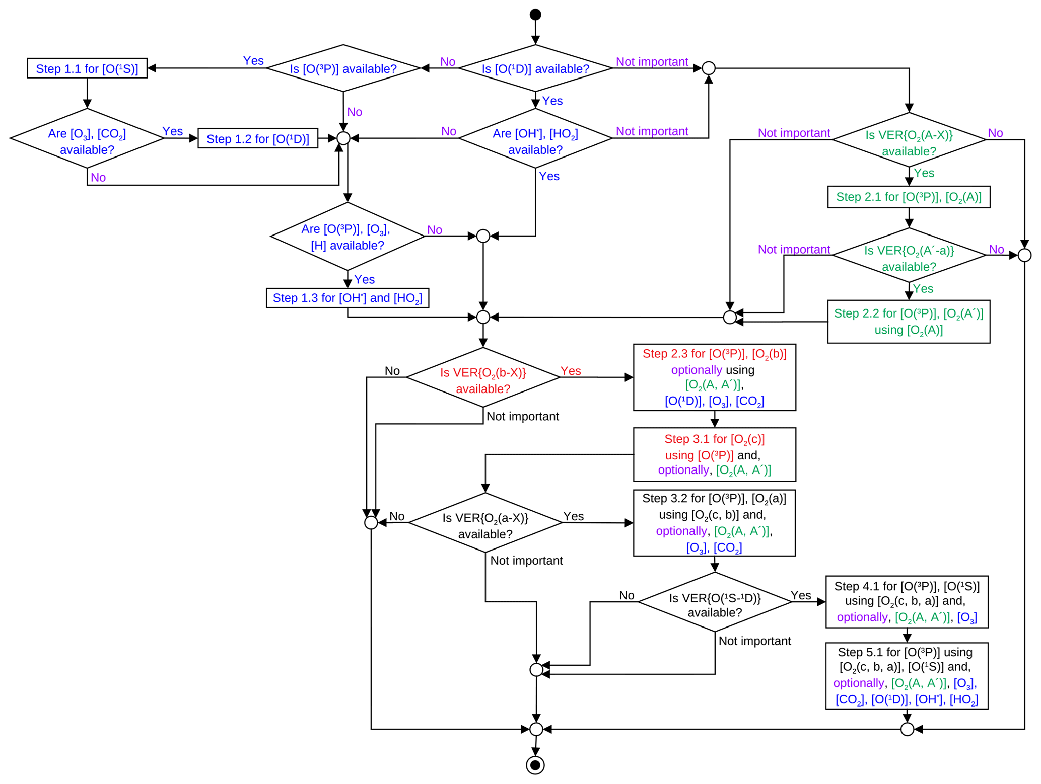
Figure A1The flowchart shows retrieval steps resulting in [O(3P)] and carried out according to the proposed MAC approach. The start and end states are denoted by filled black circles on the top and bottom of the figure, respectively. Decisions and processes are denoted by rhombs and rectangles, respectively. Connectors are denoted by empty circles. The flowchart is read following lines with arrows from one flowchart symbol to another. The prior retrieval procedure is described by the text shown in blue. If the prior retrieval procedure can be omitted (as is the case for the ETON campaign), then the corresponding decision “not important” (shown in violet) near a rhomb is to be taken, which is denoted by “optionally” (shown in violet in a rectangle) and is relevant for the optional calculation result (shown in blue in a rectangle). The optional procedure carried out to calculate [O2(A)] and [O2(A′)] is described by the text shown in green. If emissions in the Herzberg I and Chamberlain bands are not available (see “no” shown in violet near the respective rhombs) or optional (see “not important” shown in violet near the respective rhombs), then this optional procedure can be omitted at steps 2.3 and 3.1; see [O2(A)] and [O2(A′)] shown in green in the respective rectangles. Note that the [O(3P)] retrieval can be carried out most accurately if values of VER{O2(b−X)} are available, which is indicated by the text shown in red.
Retrieval steps resulting in [O(3P)] and carried out according to the proposed algorithm are illustrated in the flowchart in Fig. A1.
Processes of the MAC model are described in the following sections according to the processes of the different models adopted in the MAC model. For instance, processes of the M model (see Sect. 3.2.1) are marked by character M, those of the H model (see Sect. 3.2.2) are marked by character H and the other (complementary) processes completing the development of the MAC model are marked by character C. The complementary (or completing) processes are related to processes of the G model (see Sect. 3.1), processes introduced to implement the hypothesis of Slanger et al. (2004b) and other processes coupling O2 states with each other; see Sect. 3.3. For instance, O2(A) is only considered in complementary processes, and [O2(A)] is marked as [O2(A)-C]. Production and loss terms of O2(A) are also marked by character C as P{O2(A)-C} and L{O2(A)-C}, respectively. Considering M, H and C processes involving O2(A), the continuity equation of the second degree with respect to [O(3P)] is established and solved for [O(3P)] values on the basis of the corresponding VER profile values denoted “retrieved” values and marked with a character R, i.e., R-VER{O2(A−X)}. Then [O2(A)] values are computed using the continuity equation and denoted “calculated” values at step 2.1. Summarizing retrievals and evaluations in the following sections or elsewhere in the article, [O2(A)] values are also denoted “retrieved” values and marked with a character R, i.e., R-[O2(A)], in order to emphasize that [O2(A)] values are computed on the basis of retrieved [O(3P)] values. This notation is employed in order to avoid confusion in comparing three kinds of MAC products:
-
retrieved concentrations of chemical species obtained using all relevant reactions (retrieved concentration profiles are marked with a character R, e.g., R-[O2(A)]);
-
evaluated concentrations of chemical species obtained by dividing the R-VER profiles, which correspond to the particular chemical species, by the respective transition probability (evaluated concentration profiles are marked with a character E, e.g., E-[O2(A)]); and
-
evaluated VER values obtained by multiplying the retrieved concentrations of the respective chemical species by the respective transition probability (evaluated VER profiles are marked with a character E, e.g., E-VER{O2(A−X)}).
A1 The first retrieval step
The first retrieval step was performed in three substeps to calculate [O(1D)], [OH∗] and [HO2] prior values. As for this study, this step was omitted for calculations carried out on the basis of measurements obtained in situ during the ETON campaign (see Sect. 2) because profiles of temperature, [N2] and [O2] were obtained using the NRLMSISE-00 model. Nevertheless, measurements obtained remotely and in situ during the WAVE2004 campaign represent data sets required at the prior retrieval step applied by Lednyts'kyy et al. (2019).
Table A1Processes of the prior retrieval, continued from those shown in Table 2.
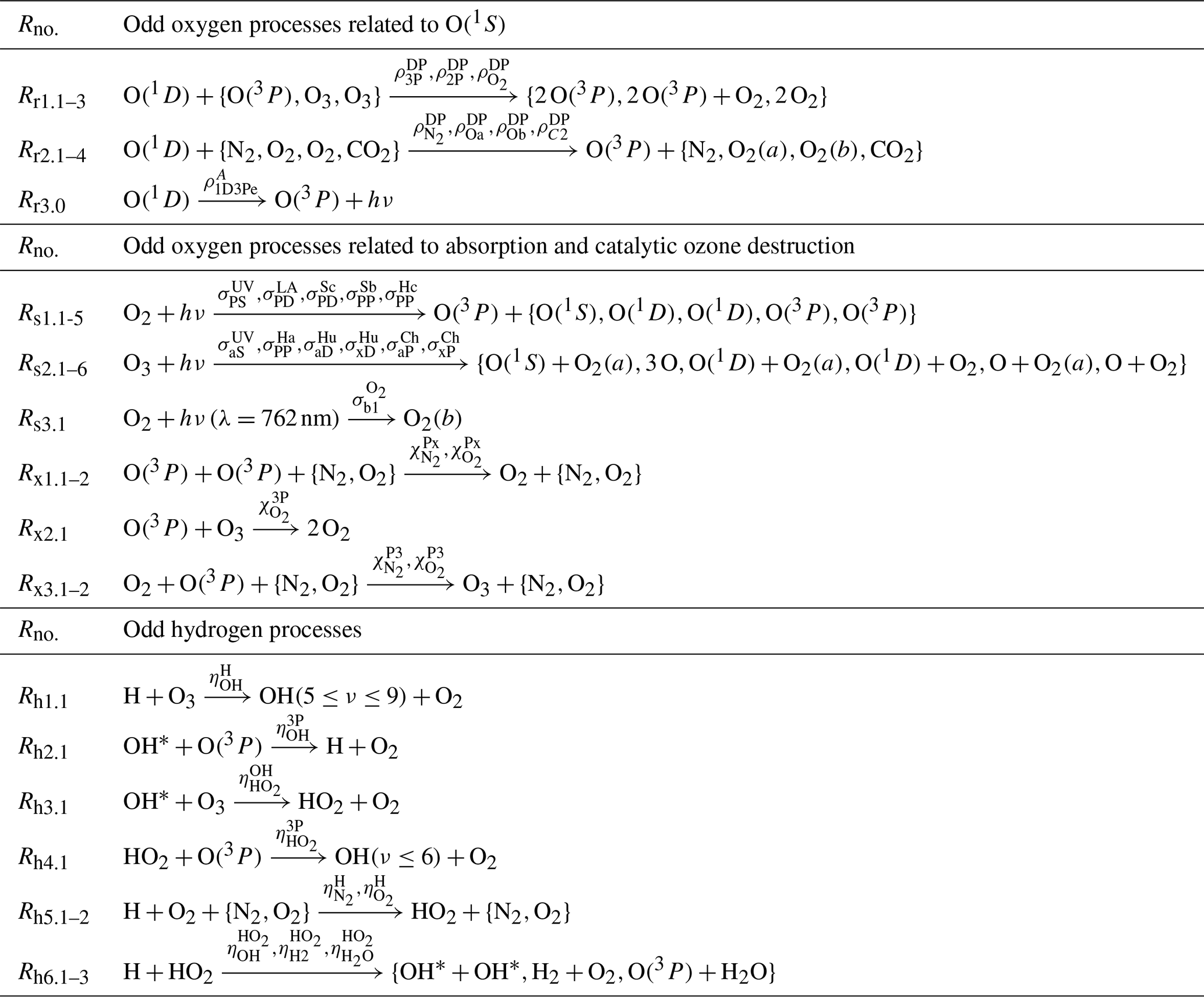
The processes shown in Tables 2 (see Sect. 3.1) and A1 were used for calculations carried out at this step. Processes marked with a character P in these tables were not used as complementary processes in the MAC model. The resulting concentration values obtained at the prior retrieval step are also marked with the character P.
A1.1 Substep 1: prior calculation of [O(1S)]
The prior calculation of [O(1S)] is performed according to the well-known cubic equation with empirical coefficients provided by McDade et al. (1986) on the basis of the in situ [O(3P)] measurements.
A1.2 Substep 2: prior calculation of [O(1D)]
The prior calculation of [O(1D)] is performed according to the corresponding continuity equation applied on the basis of [O3] and [CO2] profiles.
The continuity equation for [O(1D)] includes the terms of the [O(1D)] production (P{O(1D)}) and loss (L{O(1D)}) as follows: .
The production and loss terms were calculated according to the processes shown in Tables 2 and A1 as follows: and with the destruction term . The prior calculation results in [O(1D)] profile values as follows: P- .
A1.3 Substep 3: prior calculation of [OH∗] and [HO2]
The prior calculation of [OH∗] and [HO2] is performed according to the corresponding continuity equations applied on the basis of [O3], [H] and [O(3P)] profiles.
The continuity equation for [OH∗] including terms of the [OH∗] production (P{OH∗}) and its loss (L{OH∗}) is as follows: . The production and loss terms were calculated according to the processes shown in Tables 2 and A1 as follows: , where .
The continuity equation for [HO2] including terms of the [HO2] production (P{HO2}) and its loss (L{HO2}) is as follows: . The production and loss terms were calculated according to the processes shown in Tables 2 and A1 as follows: , where .
The system of continuity equations for [OH∗] and [HO2] was transformed to a system of the two following equations: P- and ; it was solved for the values of [HO2]. The obtained values of [HO2] were calculated as follows: P-, where .
A2 The second retrieval step
The second retrieval step was performed within four substeps to calculate [O2(b)] values.
A2.1 Substep 1: calculation of [O2(A)]
The Herzberg I band emission measured at 320 nm was used to retrieve VER{O2(A−X)} values and then to retrieve [O(3P)] values according to the continuity equation for [O2(A)], i.e., the quadratic equation with respect to [O(3P)]. Then, [O2(A)] values were retrieved (R-[O2(A)]) on the basis of [O(3P)] values by using the continuity equation considering all relevant processes of the MAC model. The continuity equation for [O2(A)] including terms of the [O2(A)] production (P{O2(A)}) and its loss (L{O2(A)}) is as follows: . The production and loss terms were calculated considering the processes shown in Tables 5 and 6 as follows: and , where . Complementary processes were used in the production and loss terms denoted with a character C. Therefore, R-[O2(A)] is also marked with the character C instead of the character R as follows: . In the case when Herzberg I band emissions are not given, [O2(A)] values can be calculated on the basis of already known [O(3P)] values.
[O2(A)] values were also evaluated (E-[O2(A)]) on the basis of retrieved VER{O2(A−X)} values (R-VER{O2(A−X)}) using the corresponding transition probability: .
Finally, VER{O2(A−X)} values were evaluated (E-VER{O2(A−X)}) on the basis of R-[O2(A)] values and the respective transition probability: .
[O2(A)] values were retrieved and then evaluated to compare and verify these calculations. VER{O2(A−X)} values were also evaluated to compare them with retrieved values in order to verify the MAC calculations; see Sect. A2.4.
A2.2 Substep 2: calculation of [O2(A′)]
The Chamberlain band emission measured at 370 nm was used to retrieve VER values and then to retrieve [O(3P)] values according to the continuity equation for [O2(A′)], i.e., the cubic equation with respect to [O(3P)]. Note that [O2(A)] values calculated at the previous step were used in the [O(3P)] retrieval at this step. Then, [O2(A′)] values were retrieved (R-[O2(A′)]) on the basis of [O(3P)] values by using the continuity equation considering all relevant processes of the MAC model. The continuity equation for [O2(A′)] including terms of the [O2(A′)] production (P{O2(A′)}) and its loss (L{O2(A′)}) is as follows: . The production and loss terms were calculated considering the processes shown in Tables 5 and 6 as follows: and , where . [O2(A′)] profile values were calculated as follows: . In the case when Chamberlain band emissions are not given, [O2(A′)] values can be calculated on the basis of already known [O(3P)] values.
[O2(A′)] values were also evaluated (E-[O2(′)]) on the basis of retrieved VER values () using the corresponding transition probability: .
Finally, VER values were evaluated () on the basis of R-[O2(A′)] values and the respective transition probability: .
[O2(A′)] values were retrieved and then evaluated to compare and verify these calculations. VER values were also evaluated to compare them with the retrieved values in order to verify the MAC calculations; see Sect. A2.4.
A2.3 Substep 3: calculation of [O2(b)]
The atmospheric band emission measured at 761.9 nm was used to retrieve VER{O2(b−X)} values and then to retrieve [O(3P)] values according to the continuity equation for [O2(b)], i.e., the cubic equation with respect to [O(3P)]. Note that [O2(A)] and [O2(A′)] values calculated at the previous steps were used in the [O(3P)] retrieval at this step. However, if the MAC model excluding O2(A) and O2(A′) is used then [O2(A)] and [O2(A′)] profile values are set to zero because these concentrations were not calculated at the previous steps. This is justified because the hypothesis of Slanger et al. (2004b) was adopted to propose the MAC model. Note that the MAC calculations were verified and validated; see Sect. 3.5 for details. Then, [O2(b)] values were retrieved (R-[O2(b)]) on the basis of [O(3P)] values by using the continuity equation considering all relevant processes of the MAC model. The continuity equation for [O2(b)] including terms of the [O2(b)] production (P{O2(b)}) and its loss (L{O2(b)}) is as follows: . The production and loss terms were calculated considering the processes shown in Tables 5 and 6.
The production term was calculated as follows: , where , , resulting in .
The loss term was calculated as follows: , where is related to the M model discussed in Sect. 3.2.1, is related to the H model discussed in Sect. 3.2.2 and corresponds to the complementary processes relevant here. Note that .
[O2(b)] values were calculated taking M, H and C processes into account as follows: , where , and , resulting in . In the case when atmospheric band emissions are not given, [O2(b)] values can be calculated on the basis of already known [O(3P)] values.
[O2(b)] values were also evaluated (E-[O2(b)]) on the basis of retrieved VER{O2(b−X)} values (R-VER{O2(b−X)}) using the corresponding transition probability: .
Finally, VER{O2(b−X)} values were evaluated (E-VER{O2(b−X)}) on the basis of R-[O2(b)] values and the respective transition probability: .
[O2(b)] values were retrieved and then evaluated to compare and verify these calculations. VER{O2(b−X)} values were also evaluated to compare them with the retrieved values in order to verify the MAC calculations; see Sect. A2.4.
A2.4 Substep 4: consistency tests in the calculation of [O2(b)]
The consistency tests in the calculations performed with the MAC model are based on the comparison of the retrieved and evaluated values.
Calculations carried out at steps 2.1 and 2.2 are relevant for the MAC model involving O2(A) and O2(A′), but calculations carried out at step 2.3 only are relevant for the MAC model excluding O2(A) and O2(A′); see the following overview.
Step 2.1 described in Sect. A2.1 was carried out to retrieve R-[O2(A)] and [O(3P)] values on the basis of R-VER{O2(A−X)} values. E-[O2(A)] values were also evaluated to compare them with R-[O2(A)] values. Additionally, E-VER{O2(A−X)} values were also evaluated to compare them with R-VER{O2(A−X)} values.
Step 2.2 described in Sect. A2.2 was carried out to retrieve R-[O2(A′)] and [O(3P)] values on the basis of and R-[O2(A)] values. E-[O2(A′)] values were also evaluated to compare them with R-[O2(A′)] values. Additionally, values were also evaluated to compare them with values.
Step 2.3 described in Sect. A2.3 was carried out with the MAC model to retrieve R-[O2(b)] and [O(3P)] values on the basis of R-VER{O2(b−X)} values. E-[O2(b)] values were also evaluated to compare them with R-[O2(b)] values. Additionally, E-VER{O2(b−X)} values were also evaluated to compare them with R-VER{O2(b−X)} values.
A3 The third retrieval step
The third retrieval step was performed in three substeps to calculate [O2(c)] and [O2(a)] values.
A3.1 Substep 1: calculation of [O2(c)]
[O2(c)] values were retrieved (R-[O2(c)]) on the basis of [O2(A)], [O2(A′)] and [O2(b)] values (obtained at steps 2.1, 2.2 and 2.3, respectively) as well as [O(3P)] values (obtained at step 2.3) according to the continuity equation for [O2(c)] considering all relevant processes of the MAC model.
The continuity equation for [O2(c)] including terms of the [O2(c)] production (P{O2(c)}) and its loss (L{O2(c)}) is as follows: . The production and loss terms were calculated considering the processes shown in Tables 5 and 6.
The production term was calculated as follows: , where P{O2(c)-M} is absent, and , resulting in .
The loss term was calculated as follows: , where L{O2(c)-M} is absent, and , resulting in .
[O2(c)] values were calculated taking M, H and C processes into account as follows: , where [O2(c)-M] is absent, and , resulting in .
A3.2 Substep 2: calculation of [O2(a)]
The infrared atmospheric band emission measured at 1.27 µm was used to retrieve VER{O2(a−X)} values and then to retrieve [O(3P)] values according to the continuity equation for [O2(a)], i.e., the cubic equation with respect to [O(3P)]. Note that [O2(A)], [O2(A′)], [O2(b)] and [O2(c)] values calculated at the previous steps were used in the [O(3P)] retrieval at this step. Then, [O2(a)] values were retrieved (R-[O2(a)]) on the basis of [O(3P)] values using the continuity equation considering all relevant processes of the MAC model. The continuity equation for [O2(a)] including terms of the [O2(a)] production (P{O2(a)}) and its loss (L{O2(a)}) is as follows: . The production and loss terms were calculated considering the processes shown in Tables 5 and 6.
The production term consists of terms related to the M model discussed in Sect. 3.2.1 (P{O2(a)-M}), to the H model discussed in Sect. 3.2.2 (P{O2(a)-H}) and the complementary processes relevant here (P{O2(a)-C}): , where , P{O2(a)-H} is absent and . The production term was calculated as follows: .
The loss term was calculated as follows: , where , L{O2(a)-H} is absent and , resulting in .
[O2(a)] values were calculated taking M, H and C processes into account as follows: , where , and , resulting in . In the case when infrared atmospheric band emissions are not given, [O2(a)] values can be calculated on the basis of already known [O(3P)] values.
[O2(a)] values were also evaluated (E-[O2(a)]) on the basis of retrieved VER{O2(a−X)} values (R-VER{O2(a−X)}) using the corresponding transition probability: .
Finally, VER{O2(a−X)} values were evaluated (E-VER{O2(a−X)}) on the basis of R-[O2(a)] values and the respective transition probability: .
[O2(a)] values were retrieved and then evaluated to compare and verify these calculations. VER{O2(a−X)} values were also evaluated to compare them with the retrieved values in order to verify the MAC calculations; see Sect. A3.3.
A3.3 Substep 3: consistency tests in the calculation of [O2(a)]
The consistency tests in the calculations performed with the MAC model are based on the comparison of the retrieved and evaluated values.
Step 3.1 described in Sect. A3.1 was carried out to retrieve R-[O2(c)] and [O(3P)] values. The corresponding calculations carried out at step 3.1 could not be tested for consistency because [O2(c)] was calculated on the basis of concentrations available from the previous steps, whereas VER profiles were not employed for the [O2(c)] calculations directly. Indeed, emissions in the Herzberg II band were not measured, whereas emissions in the new system from Keck I/II and the Richards–Johnson system have a low signal-to-noise ratio. Therefore, only calculations carried out at step 3.2 are tested for consistency.
Step 3.2 described in Sect. A3.2 was carried out to retrieve R-[O2(a)] and [O(3P)] values on the basis of R-VER{O2(a−X)} values and the concentrations of available excited chemical species. E-[O2(a)] values were also evaluated to compare them with R-[O2(a)] values. Additionally, E-VER{O2(a−X)} values were also evaluated to compare them with R-VER{O2(a−X)} values.
A4 The fourth retrieval step
The fourth retrieval step was performed in two substeps to calculate [O(1S)] values.
A4.1 Substep 1: calculation of [O(1S)]
The oxygen green line emission measured at 557.7 nm was used to retrieve VER{O(1S−1D)} values and then to retrieve [O(3P)] values according to the continuity equation for [O(1S)], i.e., the cubic equation with respect to [O(3P)]. Note that [O2(A)], [O2(A′)], [O2(c)], [O2(b)] and [O2(a)] values calculated at the previous steps were used in the [O(3P)] retrieval at this step. Then, [O(1S)] values were retrieved (R-[O(1S)]) on the basis of [O(3P)] values by using the continuity equation considering all relevant processes of the MAC model. The continuity equation for [O(1S)] including terms of the [O(1S)] production (P{O(1S)}) and its loss (L{O(1S)}) is as follows: . The production and loss terms were calculated considering the processes shown in Tables 5 and 6.
The production term consists of terms related to the M model discussed in Sect. 3.2.1 (P{O(1S)-M}), to the H model discussed in Sect. 3.2.2 (P{O(1S)-H}) and the complementary processes relevant here (P{O(1S)-C}): , where P{O(1S)-M} is absent, P{O(1S)-H}=[O(3P)]Rc2.1[O2(c)] and . The production term was calculated as follows: .
The loss term was calculated as follows: , where L{O(1S)-M} is absent, and , resulting in .
[O(1S)] values were calculated taking M, H and C processes into account as follows: , where [O(1S)-M] is absent, and [O(1S)-C] is absent. In the case when oxygen green line emissions are not given, [O(1S)] values can be calculated on the basis of already known [O(3P)] values.
[O(1S)] values were also evaluated (E-[O(1S)]) on the basis of retrieved VER{O(1S−1D)} values (R-VER{O(1S−1D)}) using the corresponding transition probability: .
Finally, VER{O(1S−1D)} values were evaluated (E-VER{O(1S−1D)}) on the basis of retrieved [O(1S)] values and the respective transition probability: .
[O(1S)] values were retrieved and then evaluated to compare and verify these calculations. VER{O(1S−1D)} values were also evaluated to compare them with the retrieved values in order to verify the MAC calculations; see Sect. A4.2.
A4.2 Substep 2: consistency tests in the calculation of [O(1S)]
The consistency tests in the calculations by using the MAC model are based on the comparison of the retrieved and evaluated values.
Step 4.1 described in Sect. A4.1 was carried out to retrieve R-[O(1S)] and [O(3P)] values on the basis of R-VER{O(1S−1D)} values and the concentrations of available excited chemical species. E-[O(1S)] values were also evaluated to compare them with R-[O(1S)] values. Additionally, E-VER{O(1S−1D)} values were also evaluated to compare them with R-VER{O(1S−1D)} values.
A5 The fifth retrieval step
The fifth retrieval step was performed to calculate [Ox] ([O(3P)], [O(1D)] and [O3]) values on the basis of the concentrations of all relevant chemical species.
A5.1 Substep 1: calculation of [O(3P)] involving all relevant chemical species
[O(3P)] values were retrieved (R-[O(3P)]) on the basis of the concentrations of atmospheric minor species calculated in the previous steps according to the continuity equation for [O(3P)] considering all relevant processes of the MAC model. For instance, values of [O2(A)], [O2(A′)], [O2(b)], [O2(c)], [O2(a)] and [O(1S)] were calculated at steps 2.1, 2.2, 2.3, 3.1, 3.2 and 4.1, respectively.
The continuity equation for [O(3P)] including terms of the [O(3P)] production (P{O(3P)}) and loss (L{O(3P)}) is as follows: . The production and loss terms were calculated considering the processes shown in Tables 5 and 6.
The production term consists of terms related to the M model discussed in Sect. 3.2.1 (P{O(3P)-M}), to the H model discussed in Sect. 3.2.2 (P{O(3P)-H}) and the complementary processes relevant here (P{O(3P)-C}): , where , and . The production term was calculated as follows: .
The loss term was calculated as follows: , where , , resulting in .
[O(3P)] values were calculated taking M, H and C processes into account as follows: , where , and .
The final equation for [O(3P)] is as follows: .
A5.2 Substep 2: calculation of [O(1D)] involving all relevant chemical species
[O(1D)] values were retrieved (R-[O(1D)]) on the basis of the concentrations of atmospheric minor species obtained at the previous steps according to the continuity equation for [O(1D)] considering all relevant processes of the MAC model.
The continuity equation for [O(1D)] including terms of the [O(1D)] production (P{O(1D)}) and loss (L{O(1D)}) is as follows: .
The production and loss terms were calculated considering the processes shown in Tables 5, 6 and 7.
The calculation of the production term was based on the considered M, H and C processes as follows: , where , P{O2(1D)-H}=Rg3.0[O(1S)] and , resulting in .
The calculation of the loss term was based on the considered M, H and C processes as follows: , where , L{O(1D)-H} is absent and , resulting in .
[O(1D)] values were calculated taking M, H and C processes into account as follows: , where , and .
The final equation for [O(1D)] is as follows: .
A5.3 Substep 3: calculation of [O3] involving all relevant chemical species
[O3] values were retrieved (R-[O3]) on the basis of the concentrations of atmospheric minor species obtained in the previous steps according to the continuity equation for [O3] considering all relevant processes of the MAC model.
The continuity equation for [O3] including terms of the [O3] production (P{O3}) and loss (L{O3}) is as follows: .
The production and loss terms were calculated considering the processes shown in Tables 5, 6 and 7.
The calculation of the production term was based on the considered M, H and C processes as follows: , where P{O3-M} is absent, P{O3-H} is absent and .
The calculation of the loss term was based on the considered M, H and C processes as follows: , where L{O3-M}=Rs2.3, L{O3-H} is absent, , resulting in .
[O3] values were calculated taking M, H and C processes into account as follows: , where [O3-M] is absent, [O3-H] is absent and .
The final equation for [O3] is as follows: .
The algorithm described in this study is available to the community and may be obtained by contacting the lead author of this article.
OL worked out the concept of the MAC approach proposed by Torr et al. (1985), developed corresponding software, performed needed computations and prepared the paper. CvS contributed to planning the work activities regarding the article, discussed the results, contributed to the paper writing, and corrected and edited it.
The authors declare that they have no conflict of interest.
The authors acknowledge the financial support provided by the German Research Foundation (DFG) through grant SA 1351/6-1 and thank Miriam Sinnhuber and Tilo Fytterer for the corresponding helpful discussions. The authors acknowledge the positive thought-provoking influence of Edward Llewellyn on working out the doctoral thesis by Olexandr Lednyts'kyy under the supervision of Christian von Savigny. Olexandr Lednyts'kyy also acknowledges the financial support provided by the University of Greifswald and the International Helmholtz Graduate School for Plasma Physics.
This research has been supported by the German Research Foundation (project number 290344289, grant no. SA 1351/6-1).
This paper was edited by William Ward and reviewed by two anonymous referees.
Ångström, J. A.: Spectrum des Nordlichts, Ann. Phys., 213, 161–163, https://doi.org/10.1002/andp.18692130510, 1869. a
Atkinson, R. and Welge, K. H.: Temperature Dependence of O(1S). Deactivation by CO2, O2, N2, and Ar, J. Chem. Phys., 57, 3689–3693, https://doi.org/10.1063/1.1678829, 1972. a, b
Atkinson, R., Baulch, D. L., Cox, R. A., Hampson, R. F., Kerr, J. A., Rossi, M. J., and Troe, J.: Evaluated kinetic and photochemical data for atmospheric chemistry: Supplement VI. IUPAC subcommittee on gas kinetic data evaluation for atmospheric chemistry, J. Phys. Chem. Ref. Data, 26, 1329–1499, 1997. a, b
Bates, D. R.: Rate of Formation of Molecules by Radiative Association, Mon. Not. R. Astron. Soc., 111, 303, https://doi.org/10.1093/mnras/111.3.303, 1951. a, b
Bates, D. R.: On the proposals of Chapman and of Barth for O(1S) formation in the upper atmosphere, Planet. Space Sci., 27, 717–718, https://doi.org/10.1016/0032-0633(79)90168-5, 1979. a, b, c
Bates, D. R.: The green light of the night sky, Planet. Space Sci., 29, 1061–1067, https://doi.org/10.1016/0032-0633(81)90003-9, 1981. a, b
Bates, D. R.: Excitation and quenching of the oxygen bands in the nightglow, Planet. Space Sci., 36, 875–881, https://doi.org/10.1016/0032-0633(88)90093-1, 1988a. a, b, c
Bates, D. R.: Special Issue: Atomic Oxygen Abundance in Thermosphere, Transition probabilities of the bands of the oxygen systems of the nightglow, Planet. Space Sci., 36, 869–873, https://doi.org/10.1016/0032-0633(88)90092-X, 1988b. a
Bovensmann, H., Burrows, J. P., Buchwitz, M., Frerick, J., Noël, S., Rozanov, V. V., Chance, K. V., and Goede, A. P. H.: SCIAMACHY: Mission Objectives and Measurement Modes, J. Atmos. Sci., 56, 127–150, https://doi.org/10.1175/1520-0469(1999)056<0127:SMOAMM>2.0.CO;2, 1999. a, b
Brasseur, G. and Solomon, S.: Aeronomy of the middle atmosphere: chemistry and physics of the stratosphere and mesosphere, Springer, Dordrecht, the Netherlands, ISBN 978-1-4020-3284-4,, 2005. a
Burkholder, J. B., Sander, S. P., Abbatt, J., Barker, J. R., Huie, R. E., Kolb, C. E., Kurylo, M. J., Orkin, V. L., Wilmouth, D. M., and Wine, P. H.: Chemical Kinetics and Photochemical Data for Use in Atmospheric Studies. Evaluation No. 18. JPL Publication 15-10, Jet Propulsion Laboratory, Pasadena, http://jpldataeval.jpl.nasa.gov/pdf/JPL_Publication_15-10.pdf (last access: 1 March 2019)), 2015. a, b, c, d, e, f, g, h
Burrows, J. P., Hölzle, E., Goede, A. P. H., Visser, H., and Fricke, W.: SCIAMACHY – scanning imaging absorption spectrometer for atmospheric chartography, Acta Astronaut., 35, 445–451, https://doi.org/10.1016/0094-5765(94)00278-T, 1995. a
Cacace, F., de Petris, G., and Troiani, A.: Experimental Detection of Tetraoxygen, Angew. Chem. Int. Edit., 40, 4062–4065, https://doi.org/10.1002/1521-3773(20011105)40:21<4062::AID-ANIE4062>3.0.CO;2-X, 2001. a
Campbell, I. M. and Gray, C. N.: Rate constants for O(3P) recombination and association with N(4S), Chem. Phys. Lett., 18, 607–609, https://doi.org/10.1016/0009-2614(73)80479-8, 1973. a, b
Capetanakis, F. P., Sondermann, F., Höser, S., and Stuhl, F.: Temperature dependence of the quenching of O(1S) by simple inorganic molecules, J. Chem. Phys., 98, 7883–7887, https://doi.org/10.1063/1.464596, 1993. a
Chapman, S.: Bakerian Lecture. Some Phenomena of the Upper Atmosphere, P. Roy. Soc. Lond. A Mat., 132, 353–374, https://doi.org/10.1098/rspa.1931.0105, 1931. a
Chapman, S.: LXVI. On the production of auroral and night-sky light, The London, Edinburgh, and Dublin Philosophical Magazine and Journal of Science, 23, 657–665, https://doi.org/10.1080/14786443708561840, 1937. a
Colegrove, F. D., Hanson, W. B., and Johnson, F. S.: Eddy diffusion and oxygen transport in the lower thermosphere, J. Geophys. Res., 70, 4931–4941, https://doi.org/10.1029/JZ070i019p04931, 1965. a, b, c, d
Cosby, P. C., Sharpee, B. D., Slanger, T. G., Huestis, D. L., and Hanuschik, R. W.: High-resolution terrestrial nightglow emission line atlas from UVES/VLT: Positions, intensities, and identifications for 2808 lines at 314–1043 nm, J. Geophys. Res.-Space, 111, 1–14, https://doi.org/10.1029/2006JA012023, A12307, 2006. a
Dudok de Wit, T., Kretzschmar, M., Lilensten, J., and Woods, T.: Finding the best proxies for the solar UV irradiance, Geophys. Res. Lett., 36, L10107, https://doi.org/10.1029/2009GL037825, 2009. a
Garcia, R. R. and Solomon, S.: The effect of breaking gravity waves on the dynamics and chemical composition of the mesosphere and lower thermosphere, J. Geophys. Res.-Atmos., 90, 3850–3868, https://doi.org/10.1029/JD090iD02p03850, 1985. a
García-Comas, M., López-Puertas, M., Marshall, B. T., Wintersteiner, P. P., Funke, B., Bermejo-Pantaleón, D., Mertens, C. J., Remsberg, E. E., Gordley, L. L., Mlynczak, M. G., and Russell, J. M.: Errors in Sounding of the Atmosphere using Broadband Emission Radiometry (SABER) kinetic temperature caused by non-local-thermodynamic-equilibrium model parameters, J. Geophys. Res.-Atmos., 113, D24106, https://doi.org/10.1029/2008JD010105, 2008. a
Gobbi, D., Takahashi, H., Clemesha, B. R., and Batista, P. P.: Equatorial atomic oxygen profiles derived from rocket observations of OI 557.7 nm airglow emission, Planet. Space Sci., 40, 775–781, https://doi.org/10.1016/0032-0633(92)90106-X, 1992. a, b, c, d, e, f, g, h, i, j
Goodman, J. and Brus, L. E.: Electronic spectroscopy and dynamics of the low-lying A, C3Δu, and c states of O2 in van der Waals solids, J. Chem. Phys., 67, 1482–1490, https://doi.org/10.1063/1.435023, 1977. a
Gordiets, B. F., Ferreira, C. M., Guerra, V. L., Loureiro, J. M. A. H., Nahorny, J., Pagnon, D., Touzeau, M., and Vialle, M.: Kinetic model of a low-pressure N2−O2 flowing glow discharge, IEEE T. Plasma Sci., 23, 750–768, https://doi.org/10.1109/27.467998, 1995. a
Greer, R. G. H., Llewellyn, E. J., Solheim, B. H., and Witt, G.: The excitation of in the nightglow, Planet. Space Sci., 29, 383–389, https://doi.org/10.1016/0032-0633(81)90081-7, 1981. a, b, c
Greer, R. G. H., Murtagh, D. P., McDade, I. C., Dickinson, P. H. G., Thomas, L., Jenkins, D. B., Stegman, J., Llewellyn, E. J., Witt, G., Mackinnon, D. J., and Williams, E. R.: ETON 1: A data base pertinent to the study of energy transfer in the oxygen nightglow, Planet. Space Sci., 34, 771–788, https://doi.org/10.1016/0032-0633(86)90074-7, 1986. a, b, c, d, e, f, g, h, i, j, k
Greer, R. G. H., Murtagh, D. P., McDade, I. C., Llewellyn, E. J., Witt, G., Thrush, B. A., Stott, I. P., and Bowhill, S. A.: Rocket photometry and the lower-thermospheric oxygen nightglow, Philos. T. Roy. Soc. A, 323, 579–595, https://doi.org/10.1098/rsta.1987.0107, 1987. a, b, c
Grygalashvyly, M., Becker, E., and Sonnemann, G. R.: Gravity Wave Mixing and Effective Diffusivity for Minor Chemical Constituents in the Mesosphere/Lower Thermosphere, Space Sci. Rev., 168, 333–362, https://doi.org/10.1007/s11214-011-9857-x, 2012. a
Grygalashvyly, M., Eberhart, M., Hedin, J., Strelnikov, B., Lübken, F.-J., Rapp, M., Löhle, S., Fasoulas, S., Khaplanov, M., Gumbel, J., and Vorobeva, E.: Atmospheric band fitting coefficients derived from a self-consistent rocket-borne experiment, Atmos. Chem. Phys., 19, 1207–1220, https://doi.org/10.5194/acp-19-1207-2019, 2019. a, b, c
Hedin, A. E.: A Revised thermospheric model based on mass spectrometer and incoherent scatter data: MSIS-83, J. Geophys. Res.-Space, 88, 10170–10188, https://doi.org/10.1029/JA088iA12p10170, 1983. a, b
Hickey, M. P., Walterscheid, R. L., Taylor, M. J., Ward, W., Schubert, G., Zhou, Q., Garcia, F., Kelly, M. C., and Shepherd, G. G.: Numerical simulations of gravity waves imaged over Arecibo during the 10-day January 1993 campaign, J. Geophys. Res.-Space, 102, 11475–11489, https://doi.org/10.1029/97JA00181, 1997. a, b, c, d
Hislop, R. J. and Wayne, R. P.: Production of in the H+O2 system, J. Chem. Soc., Faraday Trans. 2, 73, 506–516, https://doi.org/10.1039/F29777300506, 1977. a, b
Hollas, J. M.: Modern Spectroscopy, John Wiley & Sons, Chichester, UK, ISBN 978-0-470-84416-8, 2004. a
Huang, T.-Y. and George, R.: Simulations of gravity wave-induced variations of the OH(8,3), O2(0,1), and O(1S) airglow emissions in the MLT region, J. Geophys. Res.-Space, 119, 2149–2159, https://doi.org/10.1002/2013JA019296, 2014. a, b, c, d, e, f, g, h, i, j, k
Huestis, D. L.: Current Laboratory Experiments for Planetary Aeronomy, American Geophysical Union, 245–258, https://agupubs.onlinelibrary.wiley.com/doi/pdf/10.1029/130GM16 (last access: 1 March 2019), 2002. a, b, c, d, e, f, g, h, i, j, k, l, m
Johnston, J. E. and Broadfoot, A. L.: Midlatitude observations of the night airglow: Implications to quenching near the mesopause, J. Geophys. Res.-Space, 98, 21593–21603, https://doi.org/10.1029/93JA02318, 1993. a
Jones, D. B., Campbell, L., Bottema, M. J., Teubner, P. J. O., Cartwright, D. C., Newell, W. R., and Brunger, M. J.: Electron-driven excitation of O2 under night-time auroral conditions: Excited state densities and band emissions, Planet. Space Sci., 54, 45–59, https://doi.org/10.1016/j.pss.2005.08.007, 2006. a
Kenner, R. D. and Ogryzlo, E. A.: A direct determination of the rate constant for the quenching of O(1S) by O2(a1Δg), J. Photochem., 18, 379–382, https://doi.org/10.1016/0047-2670(82)87027-5, 1982. a, b, c, d
Kenner, R. D. and Ogryzlo, E. A.: Quenching of by O(3P), O2(a1Δg), and other gases, Can. J. Chem., 61, 921–926, https://doi.org/10.1139/v83-165, 1983. a, b
Kenner, R. D. and Ogryzlo, E. A.: Quenching of the Herzberg I band by O2(a) and O, Can. J. Phys., 62, 1599–1602, https://doi.org/10.1139/p84-204, 1984. a
Khomich, V. Y., Semenov, A. I., and Shefov, N. N.: Airglow as an indicator of upper atmospheric structure and dynamics, Springer, Berlin, Heidelberg, Germany, ISBN 978-3-540-75832-7, 2008. a, b, c, d, e, f, g, h, i, j
Kramida, A., Ralchenko, Y., Reader, J., Sansonetti, J. E., and NIST, A. T.: NIST Atomic Spectra Database (version 5.3), available at: http://physics.nist.gov/asd (last access: 1 March 2019), 2015. a
Krasnopolsky, V. A.: Excitation of oxygen emissions in the night airglow of the terrestrial planets, Planet. Space Sci., 29, 925–929, https://doi.org/10.1016/0032-0633(81)90053-2, 1981. a, b, c, d
Krasnopolsky, V. A.: Oxygen emissions in the night airglow of the Earth, Venus and Mars, Planet. Space Sci., 34, 511–518, https://doi.org/10.1016/0032-0633(86)90089-9, 1986. a, b, c
Krasnopolsky, V. A.: Excitation of the oxygen nightglow on the terrestrial planets, Planet. Space Sci., 59, 754–766, https://doi.org/10.1016/j.pss.2011.02.015, 2011. a, b, c, d, e, f, g, h, i
Krauss, M. and Neumann, D.: On the interaction of O(1S) with O(3P), Chem. Phys. Lett., 36, 372–374, https://doi.org/10.1016/0009-2614(75)80259-4, 1975. a, b
Lakowicz, J. R.: Principles of Fluorescence Spectroscopy, Springer US, New York, USA, ISBN 978-0-387-31278-1, https://doi.org/10.1007/978-0-387-46312-4, 2006. a, b, c, d
Lednyts'kyy, O. and von Savigny, C.: Development of a Multiple Airglow Chemistry model and validation with in-situ Airglow Measurements, Midterm HEPP Meeting of the Max Planck Society, Berlin, Germany, 27 October 2016, N1, 2016. a, b, c, d, e, f, g, h, i, j, k
Lednyts'kyy, O., von Savigny, C., Eichmann, K.-U., and Mlynczak, M. G.: Atomic oxygen retrievals in the MLT region from SCIAMACHY nightglow limb measurements, Atmos. Meas. Tech., 8, 1021–1041, https://doi.org/10.5194/amt-8-1021-2015, 2015. a, b, c, d, e, f, g, h, i, j, k, l, m, n, o, p, q, r, s
Lednyts'kyy, O., von Savigny, C., and Weber, M.: Sensitivity of equatorial atomic oxygen in the MLT region to the 11-year and 27-day solar cycles, J. Atmos. Sol.-Terr. Phy., 162, 136–150, https://doi.org/10.1016/j.jastp.2016.11.003, 2017. a
Lednyts'kyy, O., von Savigny, C., and Llewellyn, E.: Validation of the extended Multiple Airglow Chemistry model with in-situ measurements of the Energy Transfer in the Oxygen Nightglow campaign, Spring Meeting of the German Physical Society, Erlangen, Germany, 4–9 March 2018, UP 8.5, 2018. a, b, c
Lednyts'kyy, O., von Savigny, C., Sinnhuber, M., Iwagami, N., and Mlynczak, M.: Multiple Airglow Chemistry approach for atomic oxygen retrievals on the basis of in situ nightglow emissions, J. Atmos. Sol.-Terr. Phy., 194, 105096, https://doi.org/10.1016/j.jastp.2019.105096, 2019. a, b, c, d
Llewellyn, E. J. and McDade, I. C.: Singlet molecular oxygen in planetary atmospheres, J. Photochem., 25, 379–388, https://doi.org/10.1016/0047-2670(84)87039-2, 1984. a, b, c
Llewellyn, E. J. and Solheim, B. H.: The excitation of the infrared atmospheric oxygen bands in the nightglow, Planet. Space Sci., 26, 533–538, https://doi.org/10.1016/0032-0633(78)90044-2, 1978. a, b, c
Llewellyn, E. J., Solheim, B. H., Witt, G., Stegman, J., and Greer, R. G. H.: On the excitation of oxygen emissions in the airglow of the terrestrial planets, J. Photochem., 12, 179–183, https://doi.org/10.1016/0047-2670(80)85041-6, 1980. a
López-González, M. J., López-Moreno, J. J., and Rodrigo, R.: Altitude and vibrational distribution of the O2 ultraviolet nightglow emissions, Planet. Space Sci., 40, 913–928, https://doi.org/10.1016/0032-0633(92)90132-8, 1992a. a, b, c
López-González, M. J., López-Moreno, J. J., and Rodrigo, R.: Altitude profiles of the atmospheric system of O2 and of the green line emission, Planet. Space Sci., 40, 783–795, https://doi.org/10.1016/0032-0633(92)90107-Y, 1992b. a, b, c, d
Makhlouf, U. B., Picard, R. H., Winick, J. R., and Tuan, T. F.: A model for the response of the atomic oxygen 557.7 nm and the OH Meinel airglow to atmospheric gravity waves in a realistic atmosphere, J. Geophys. Res.-Atmos., 103, 6261–6269, https://doi.org/10.1029/97JD03082, 1998. a, b, c
McConkey, J. W., Burns, D. J., Moran, K. A., and Emeleus, K. G.: Measurement of relative multipole transition probabilities in atomic oxygen, Phys. Lett., 22, 416–417, https://doi.org/10.1016/0031-9163(66)91206-6, 1966. a
McDade, I. C.: The photochemistry of the MLT oxygen airglow emissions and the expected influences of tidal perturbations, Adv. Space Res., 21, 787–794, https://doi.org/10.1016/S0273-1177(97)00674-1, 1998. a
McDade, I. C., Murtagh, D. P., Greer, R. G. H., Dickinson, P. H. G., Witt, G., Stegman, J., Llewellyn, E. J., Thomas, L., and Jenkins, D. B.: ETON 2: Quenching parameters for the proposed precursors of and O(1S) in the terrestrial nightglow, Planet. Space Sci., 34, 789–800, https://doi.org/10.1016/0032-0633(86)90075-9, 1986. a, b, c, d, e, f, g, h, i, j, k, l, m, n, o, p, q, r, s, t, u, v, w, x, y, z, aa, ab, ac, ad, ae, af, ag, ah, ai, aj, ak
Meier, R. R.: Ultraviolet spectroscopy and remote sensing of the upper atmosphere, Space Sci. Rev., 58, 1–185, https://doi.org/10.1007/BF01206000, 1991. a
Meinel, A. B.: O2 Emission Bands in the Infrared Spectrum of the Night Sky, Astrophys. J., 112, 464–468, https://doi.org/10.1086/145360, 1950. a
Minaev, B. F. and Ågren, H.: Collision-induced , , transition probabilities in molecular oxygen, J. Chem. Soc., 93, 2231–2239, 1997. a
Mlynczak, M. G., Solomon, S., and Zaras, D. S.: An updated model for O2(a1Δg) concentrations in the mesosphere and lower thermosphere and implications for remote sensing of ozone at 1.27 µm, J. Geophys. Res.-Atmos., 98, 18639–18648, https://doi.org/10.1029/93JD01478, 1993. a, b, c, d, e, f, g, h, i, j
Murtagh, D., Witt, G., Stegman, J., McDade, I., Llewellyn, E., Harris, F., and Greer, R.: An assessment of proposed O(1S) and nightglow excitation parameters, Planet. Space Sci., 38, 43–53, https://doi.org/10.1016/0032-0633(90)90004-A, 1990. a, b, c, d, e
Nagy, A. F., Balogh, A., Cravens, T. E., Mendillo, M., and Müller-Wodarg, I.: Comparative Aeronomy, Springer-Verlag, New York, USA, 267–310, https://doi.org/10.1007/978-0-387-87825-6, 2008. a
Nicolet, M.: Aeronomic reactions of hydrogen and ozone. In: Mesospheric model and related experiments, pp. 1–51, D. Reidel Publishing Company, Dordrecht, the Netherlands, https://doi.org/10.1007/978-94-010-3114-1, 1971. a
Nicolet, M.: Aeronomic chemistry of ozone, Planet. Space Sci., 37, 1621–1652, https://doi.org/10.1016/0032-0633(89)90150-5, 1989. a
Nicolet, M. and Kennes, R.: Aeronomic problems of molecular oxygen photodissociation IV. The various parameters for the Herzberg continuum, Planet. Space Sci., 36, 1069–1076, https://doi.org/10.1016/0032-0633(88)90044-X, 1988. a
Nicolet, M., Cleslik, S., and Kennes, R.: Aeronomic problems of molecular oxygen photodissociation V. Predissociation in the Schumann-Runge bands of oxygen, Planet. Space Sci., 37, 427–458, https://doi.org/10.1016/0032-0633(89)90124-4, 1989. a
Pejaković, D. A., Copeland, R. A., Cosby, P. C., and Slanger, T. G.: Studies on the production of and from collisional removal of , J. Geophys. Res.-Space, 112, A10307, https://doi.org/10.1029/2007JA012520, 2007. a
Pendleton, W. R., Baker, D. J., Reese, R. J., and O'Neil, R. R.: Decay of O2(a1Δg) in the evening twilight airglow: Implications for the radiative lifetime, Geophys. Res. Lett., 23, 1013–1016, https://doi.org/10.1029/96GL00946, 1996. a
Picone, J. M., Hedin, A. E., Drob, D. P., and Aikin, A. C.: NRLMSISE-00 empirical model of the atmosphere: Statistical comparisons and scientific issues, J. Geophys. Res.-Space, 107, 1468, https://doi.org/10.1029/2002JA009430, 2002. a
Pinheiro, M. J., Gousset, G., Granier, A., and Ferreira, C. M.: Modelling of low-pressure surface wave discharges in flowing oxygen: I. Electrical properties and species concentrations, Plasma Sources Science and Technology, 7, 524, https://doi.org/10.1088/0963-0252/7/4/010, 1998. a
Predoi-Cross, A., Hambrook, K., Keller, R., Povey, C., Schofield, I., Hurtmans, D., Over, H., and Mellau, G. C.: Spectroscopic lineshape study of the self-perturbed oxygen A-band, J. Mol. Spectrosc., 248, 85–110, https://doi.org/10.1016/j.jms.2007.11.007, 2008. a
Qian, L., Solomon, S. C., and Kane, T. J.: Seasonal variation of thermospheric density and composition, J. Geophys. Res.-Space, 114, https://doi.org/10.1029/2008JA013643, 2009. a
Remsberg, E. E., Marshall, B. T., García-Comas, M., Krueger, D., Lingenfelser, G. S., Martin-Torres, J., Mlynczak, M. G., Russell, J. M., Smith, A. K., Zhao, Y., Brown, C., Gordley, L. L., López-González, M. J., López-Puertas, M., She, C.-Y., Taylor, M. J., and Thompson, R. E.: Assessment of the quality of the Version 1.07 temperature-versus-pressure profiles of the middle atmosphere from TIMED/SABER, J. Geophys. Res.-Atmos., 113, D17101, https://doi.org/10.1029/2008JD010013, 2008. a
Rezac, L., Kutepov, A., Russell III, J. M., Feofilov, A. G., Yue, J., and Goldberg, R. A.: Simultaneous retrieval of T(p) and CO2 VMR from two-channel non-LTE limb radiances and application to daytime SABER/TIMED measurements, J. Atmos. Sol.-Terr. Phy., 130–131, 23–42, https://doi.org/10.1016/j.jastp.2015.05.004, 2015. a
Roble, R. G.: Energetics of the Mesosphere and Thermosphere, American Geophysical Union, 1–21, https://doi.org/10.1029/GM087p0001, 2013. a
Rodrigo, R., López-Moreno, J. J., López-Puertas, M., and Molina, A.: Progress in Atmospheric Physics, Kluwer Academic Publishers, 3–31, available at: https://www.springer.com/gp/book/9789027727534 (last access: 1 March 2019), 1988. a
Sakai, J., Hosokawa, K., Taguchi, S., and Ogawa, Y.: Storm time enhancements of 630.0 nm airglow associated with polar cap patches, J. Geophys. Res.-Space, 119, 2214–2228, https://doi.org/10.1002/2013JA019197, 2014. a
Sandu, A. and Sander, R.: Technical note: Simulating chemical systems in Fortran90 and Matlab with the Kinetic PreProcessor KPP-2.1, Atmos. Chem. Phys., 6, 187–195, https://doi.org/10.5194/acp-6-187-2006, 2006. a
Semenov, A. I.: Long-term changes in the height profiles of ozone and atomic oxygen in the lower thermosphere, Geomagn. Aeronomy+, 37, 354–360, 1997. a, b, c, d, e, f, g, h
Sharma, R. D., Wintersteiner, P. P., and Kalogerakis, K. S.: A new mechanism for OH vibrational relaxation leading to enhanced CO2 emissions in the nocturnal mesosphere, Geophys. Res. Lett., 42, 4639–4647, https://doi.org/10.1002/2015GL063724, 2015. a, b
Sharp, W. E., Zaccheo, T. S., Browell, E. V., Ismail, S., Dobler, J. T., and Llewellyn, E. J.: Impact of ambient O2(a1Δg) on satellite-based laser remote sensing of O2 columns using absorption lines in the 1.27 µm region, J. Geophys. Res.-Atmos., 119, 7757–7772, https://doi.org/10.1002/2013JD021324, 2014. a, b, c, d, e, f
Shematovich, V. I., Bisikalo, D. V., Krauss, S., Hausleitner, W., and Lammer, H.: Influence of the hot oxygen corona on the satellite drag in the Earth's upper atmosphere, Solar Syst. Res.+, 45, 231–239, https://doi.org/10.1134/S003809461103004X, 2011. a, b
Slanger, T. G.: Generation of from oxygen atom recombination, J. Chem. Phys., 69, 4779–4791, https://doi.org/10.1063/1.436504, 1978. a
Slanger, T. G. and Copeland, R. A.: Energetic Oxygen in the Upper Atmosphere and the Laboratory, Chem. Rev., 103, 4731–4766, https://doi.org/10.1021/cr0205311, 2003. a, b, c
Slanger, T. G., Cosby, P. C., and Huestis, D. L.: A new O2 band system: The – transition in the terrestrial nightglow, J. Geophys. Res.-Space, 108, 1089, https://doi.org/10.1029/2002JA009677, 2004a. a
Slanger, T. G., Cosby, P. C., and Huestis, D. L.: Co-variation of nightglow emission from the and states and the oxygen green line, observed with the Keck I/II telescopes, J. Atmos. Sol.-Terr. Phy., 66, 617–622, https://doi.org/10.1016/j.jastp.2004.01.013, 2004b. a, b, c, d, e, f, g, h, i, j, k, l, m, n, o, p, q, r, s
Smith, G. P. and Robertson, R.: Temperature dependence of oxygen atom recombination in nitrogen after ozone photolysis, Chem. Phys. Lett., 458, 6–10, https://doi.org/10.1016/j.cplett.2008.04.074, 2008. a, b, c, d
Smith, I. W. M.: The role of electronically excited states in recombination reactions, Int. J. Chem. Kinet., 16, 423–443, https://doi.org/10.1002/kin.550160411, 1984. a
Solheim, B. H. and Llewellyn, E. J.: An indirect mechanism for the production of O(1S) in the aurora, Planet. Space Sci., 27, 473–479, https://doi.org/10.1016/0032-0633(79)90124-7, 1979. a
Solomon, S. C. and Qian, L.: Solar extreme-ultraviolet irradiance for general circulation models, J. Geophys. Res.-Space, 110, 1–14, https://doi.org/10.1029/2005JA011160, 2005. a, b
Steadman, J. A. and Thrush, B. A.: A laboratory study of the mechanism of the oxygen airglow, J. Atmos. Chem., 18, 301–317, https://doi.org/10.1007/BF00712449, 1994. a, b, c, d, e
Stegman, J. and Murtagh, D. P.: The molecular oxygen band systems in the U. V. nightglow: Measured and modelled, Planet. Space Sci., 39, 595–609, https://doi.org/10.1016/0032-0633(91)90054-E, 1991. a
Stott, I. P. and Thrush, B. A.: Laboratory studies of the mechanism of the oxygen airglow, P. Roy. Soc. Lond. A Mat., 424, 1–17, https://doi.org/10.1098/rspa.1989.0066, 1989. a, b, c, d, e
Swenson, G., Yee, Y., Vargas, F., and Liu, A.: Vertical diffusion transport of atomic oxygen in the mesopause region consistent with chemical losses and continuity: Global mean and inter-annual variability, J. Atmos. Sol.-Terr. Phy., 178, 47 – 57, https://doi.org/10.1016/j.jastp.2018.05.014, 2018. a
Thomas, R. J.: Atomic hydrogen and atomic oxygen density in the mesopause region: Global and seasonal variations deduced from Solar Mesosphere Explorer near-infrared emissions, J. Geophys. Res.-Atmos., 95, 16457–16476, https://doi.org/10.1029/JD095iD10p16457, 1990. a
Torr, M. R., Torr, D. G., and Laher, R. R.: The O2 atmospheric 0-0 band and related emissions at night from Spacelab 1, J. Geophys. Res.-Space, 90, 8525–8538, https://doi.org/10.1029/JA090iA09p08525, 1985. a, b, c, d, e, f
Trajmar, S., Williams, W., and Kuppermann, A.: Angular Dependence of Electron Impact Excitation Cross Sections of O2, J. Chem. Phys., 56, 3759–3765, https://doi.org/10.1063/1.1677774, 1972. a, b
von Savigny, C. and Lednyts'kyy, O.: On the relationship between atomic oxygen and vertical shifts between OH Meinel bands originating from different vibrational levels, Geophys. Res. Lett., 40, 5821–5825, https://doi.org/10.1002/2013GL058017, 2013. a
von Savigny, C., Lednyts'kyy, O., Forbes, J. M., and Zhang, X.: Lunar semidiurnal tide in the terrestrial airglow, Geophys. Res. Lett., 42, 3553–3559, https://doi.org/10.1002/2015GL063567, 2015. a
Wayne, R. P.: Singlet oxygen in the environmental sciences, Res. Chem. Intermediat., 20, 395–422, https://doi.org/10.1163/156856794X00397, 1994. a, b
Wei, Y., Pu, Z., Zong, Q., Wan, W., Ren, Z., Fraenz, M., Dubinin, E., Tian, F., Shi, Q., Fu, S., and Hong, M.: Oxygen escape from the Earth during geomagnetic reversals: Implications to mass extinction, Earth Planet. Sc. Lett., 394, 94–98, https://doi.org/10.1016/j.epsl.2014.03.018, 2014. a, b
Wraight, P. C.: Association of atomic oxygen and airglow excitation mechanisms, Planet. Space Sci., 30, 251–259, https://doi.org/10.1016/0032-0633(82)90003-4, 1982. a
Yankovsky, V. A., Kuleshova, V. A., Manuilova, R. O., and Semenov, A. O.: Retrieval of total ozone in the mesosphere with a new model of electronic-vibrational kinetics of O3 and O2 photolysis products, Izv. Atmos. Ocean. Phy.+, 43, 514–525, https://doi.org/10.1134/S0001433807040135, 2007. a
Yankovsky, V. A., Martyshenko, K. V., Manuilova, R. O., and Feofilov, A. G.: Oxygen dayglow emissions as proxies for atomic oxygen and ozone in the mesosphere and lower thermosphere, J. Mol. Spectrosc., 327, 209–231, https://doi.org/10.1016/j.jms.2016.03.006, 2016. a, b
- Abstract
- Introduction
- Data sets applied in the Multiple Airglow Chemistry (MAC) model
- Development of the MAC model
- Discussion of the obtained results
- Conclusions
- Appendix A: Algorithmic steps of the Multiple Airglow Chemistry model development
- Code availability
- Author contributions
- Competing interests
- Acknowledgements
- Financial support
- Review statement
- References