the Creative Commons Attribution 4.0 License.
the Creative Commons Attribution 4.0 License.
 | 26 Feb 2020
The day-to-day co-variability between mineral dust and cloud glaciation: a proxy for heterogeneous freezing
Diego Villanueva
Bernd Heinold
Patric Seifert
Hartwig Deneke
Martin Radenz
Ina Tegen
To estimate the global co-variability between mineral dust aerosol and cloud glaciation, we combined an aerosol model reanalysis with satellite retrievals of cloud thermodynamic phase. We used the CALIPSO-GOCCP product from the A-Train satellite constellation to assess whether clouds are composed of liquid or ice and the MACC reanalysis to estimate the dust mixing ratio in the atmosphere. Night-time retrievals within a temperature range from +3 to −42 ∘C for the period 2007–2010 were included. The results confirm that the cloud thermodynamic phase is highly dependent on temperature and latitude. However, at middle and high latitudes, at equal temperature and within narrow constraints for humidity and static stability, the average frequency of fully glaciated clouds increases by +5 to +10 % for higher mineral dust mixing ratios. The discrimination between humidity and stability regimes reduced the confounding influence of meteorology on the observed relationship between dust and cloud ice. Furthermore, for days with similar mixing ratios of mineral dust, the cloud ice occurrence frequency in the Northern Hemisphere was found to be higher than in the Southern Hemisphere at −30 ∘C but lower at −15 ∘C. This contrast may suggest a difference in the susceptibility of cloud glaciation to the presence of dust. Based on previous studies, the differences at −15 ∘C could be explained by higher feldspar fractions in the Southern Hemisphere, while the higher freezing efficiency of clay minerals in the Northern Hemisphere may explain the differences at −30 ∘C.
- Article
(3109 KB) - Full-text XML
-
Supplement
(11824 KB) - BibTeX
- EndNote


Aerosol–cloud interactions affect the Earth’s climate through different mechanisms. These include impacts of aerosol particles on cloud glaciation that subsequently influence the clouds’ thermodynamic phase, albedo, lifetime, and precipitation. Specifically, there is growing evidence for a role of mineral dust aerosol (or of ice-nucleating particles correlated to dust aerosol) in influencing heterogeneous cloud ice formation on a global scale (Boose et al., 2016; Kanitz et al., 2011; Seifert et al., 2010; Tan et al., 2014; Vergara-Temprado et al., 2017; Zhang et al., 2018). Cloud droplets can freeze heterogeneously between 0 and −42 ∘C after interacting with ice-nucleating particles (INPs) or already existing ice particles (Hoose and Möhler, 2012). It has been shown that specific aerosol types such as mineral dust and biogenic particles can act efficiently as INPs already at temperatures between −10 and −20 ∘C (Atkinson et al., 2013). Mineral dust aerosol is emitted from arid regions, mainly from the Sahara and Asian deserts. Despite this, several dust sources exist in the southern mid-latitudes (e.g. Patagonia, South Africa, and Australia), and simulations show that long-range transport of dust, although sporadic, can result in considerable dust concentrations even in remote areas (Albani et al., 2012; Johnson et al., 2011; Li et al., 2008; Vergara-Temprado et al., 2017). Mineral dust aerosol is therefore suspected to be a principal contributor to the atmospheric INP reservoir, especially in the Northern Hemisphere, where the mixing ratio of dust aerosol is typically 1 to 2 orders of magnitude larger than in the Southern Hemisphere (Vergara-Temprado et al., 2018).
The dust occurrence frequency retrieved from spaceborne instruments like the Cloud-Aerosol LIdar with Orthogonal Polarization (CALIOP; Wu et al., 2014) has been previously used to assess the spatial correlation between dust and cloud thermodynamic phase (Choi et al., 2010; Li et al., 2017a; Tan et al., 2014). Two main problems arise from this approach. First, lidar instruments cannot detect aerosol within and below thick clouds. Second, low dust concentrations usually fall below the lower detection limit of CALIOP. The AErosol RObotic NETwork (AERONET; Dubovik et al., 2000), a network of ground-based remote sensing stations, has been used to evaluate and validate the dust retrievals from CALIOP. The stations from the AERONET mission use sun photometers to measure the spectrum of the solar irradiance and sky radiance to determine the atmospheric aerosol optical thickness (AOT). It has been shown that the CALIOP level 2 data misses about half of the dust aerosol events detected by AERONET when the AOT is less than 0.05 (Toth et al., 2018). However, dust loadings simulated by state-of-the-art models show that most of the regions in the Southern Hemisphere have an annual mean AOT lower than 0.01 (Ridley et al., 2016).
Ice particles and cloud droplets may coexist in a so-called mixed-phase state (Korolev et al., 2017). Shallow mixed-phase clouds with a liquid-dominated cloud top and ice virgae beneath are very frequent (Zhang et al., 2010), and they are generally observed down to temperatures of −25 ∘C (Ansmann et al., 2008; De Boer et al., 2011; Westbrook and Illingworth, 2011). However, ground-based and satellite retrievals are not yet able to accurately estimate the mass ratio of the cloud liquid and ice phases, especially in these liquid-dominated cloud top layers. Therefore, the frequency phase ratio (FPR) is often used instead (Cesana et al., 2015; Cesana and Chepfer, 2013; Hu et al., 2010). For satellite retrievals, this is defined as the ratio of ice voxels to total cloudy voxels for a certain volume in the atmosphere. Because most retrievals classify the cloud thermodynamic phase either as pure ice or pure supercooled liquid, the average of the FPR represents the ratio of glaciated clouds with respect to total cloud occurrence. Therefore, the FPR should not be confused with the ice-to-liquid mass ratio within a cloud volume. Cloud phase in the Northern Hemisphere and Southern Hemisphere has been studied in terms of FPR both by ground-based lidar (Kanitz et al., 2011) and by different spaceborne instruments (Choi et al., 2010; Morrison et al., 2011; Tan et al., 2014; Zhang et al., 2018). These studies found significant differences between the two hemispheres. In these studies, it has been suggested that such differences are related to differences in aerosol and INP concentrations. Moreover, the local FPR measured at various temperatures between 3 and −42 ∘C by a lidar in central Europe over a time span of 11 years has been shown to increase for higher dust loadings (Seifert et al., 2010). Furthermore, the cloud thermodynamic phase and aerosol occurrence frequency – both retrieved from a spaceborne lidar – are spatially correlated, especially at temperatures of around −20 ∘C (Choi et al., 2010; Tan et al., 2014; Zhang et al., 2012, 2015). This spatial correlation has been found under different atmospheric conditions, including humidity, surface temperature, vertical velocity, thermal stability, and zonal wind speed (Li et al., 2017a). However, the analysis of the temporal variability of cloud thermodynamic phase has received less attention, especially in remote areas like the Southern Ocean (Vergara-Temprado et al., 2017). Specifically, it is possible to study the temporal correlation between dust aerosol and cloud ice with a daily resolution. This kind of correlation is known as day-to-day correlation (inter-daily) to avoid confusion with the intra-daily variability (diurnal cycle). Additionally, a more comprehensive and quantitative assessment of the potential effect of mineral dust on cloud glaciation is currently lacking.
In this study, we use a global aerosol reanalysis together with the cloud thermodynamic phase retrievals of the CALIPSO-GOCCP (GCM-Oriented Cloud Calipso Product; Cesana and Chepfer, 2013). We use a ranked correlation approach, separating the cloud phase retrievals into different deciles of dust aerosol loading. Additionally, we separate the retrievals into different humidity and stability regimes to constrain artefacts due to meteorological factors.
In Sect. 2, the datasets used for the study are presented. In Sect. 3, the processing of the datasets are described. In Sect. 4, the main findings are presented, including a case study, the distribution of cloud phase along temperature and latitude, and finally the day-to-day correlation between dust and cloud ice. In Sect. 5, the main overlaps and differences with respect to previous findings are discussed and put into context with the conceptual limitations of the approach.
This section presents an overview of the datasets used in this study. The cloud thermodynamic phase is obtained from the CALIPSO-GOCCP product, the aerosol information from the MACC reanalysis, and the large-scale meteorological conditions from the ERA-Interim reanalysis.
2.1 CALIPSO-GOCCP
The CALIPSO-GOCCP v.3.0 product (Cesana and Chepfer, 2013) uses the attenuated total backscatter (ATB), the molecular ATB (ATBmol), and the cross-polarized ATB from CALIOP at 532 nm wavelength to detect cloudy voxels. The lidar has a horizontal resolution of 333 m and a vertical resolution of 30 m; however, the cloud properties in the CALIPSO-GOCCP product are retrieved at a vertical resolution of 480 m. The nadir angle of CALIOP was increased from 0.3 to 3∘ in November 2007 to reduce specular returns from horizontally oriented ice crystals. In the product, cloudy voxels – of 480 m height – are defined as voxels with a scattering ratio (SR) higher than five (SR = ATB/ATBmol>5). Then, the cloud volume fraction at each level is defined as the ratio of cloudy to total voxels within a m volume grid box. The product uses the depolarization ratio of the retrieved signal components to make a decision on cloud phase (ice or liquid). The decision is based on an empirical threshold for the depolarization ratio of ice particles and is made for each cloudy voxel. From this information, the FPR is calculated as the ratio of ice voxels to the total number of voxels within each m volume grid box. Instead of the 480 m levels, we use the temperature levels of the CALIPSO-GOCCP product, which uses 3 K temperature bins as a vertical coordinate. In this case, the temperature profiles are obtained from the Modern Era Retrospective analysis for Research and Applications (MERRA; Bosilovich et al., 2011) reanalysis.
2.2 MACC and ERA-Interim reanalyses
The Monitoring Atmospheric Composition and Climate reanalysis (MACC; Eskes et al., 2015) is based on the Integrated Forecast System (IFS) of the European Centre for Medium-Range Weather Forecasts (ECMWF) and simulates the emission, transport, and deposition of various aerosol species and trace gases with an output resolution of and 60 vertical levels. In this study, we use the dust mixing ratio and large-scale vertical velocity from the daily MACC reanalysis product on model levels provided by the ECMWF. Additionally, the relative humidity (RH) from the ERA-Interim reanalysis daily product (Dee et al., 2011) is used in Sect. 5. The cloud properties in the MACC reanalysis are derived from the ECMWF Integrated Forecast System (IFS Cycle 36r1 4D-Var). This atmospheric model is analogous to the one used in the ERA-Interim reanalysis (IFS Cycle 31r2 4D-Var). At the time of this study, the new generation of reanalysis based on IFS Cycle 41r was not yet publicly available. However, it is expected that future studies will use the new CAMS (Copernicus Atmosphere Monitoring Service) and ERA5 reanalysis instead of the MACC and Era-Interim reanalyses.
The averaged meteorological parameters (RH, large-scale updraught, and isotherm height) used in Sect. 5 were weighted by the cloud volume fraction retrieved by the CALIPSO-GOCCP product (see Sect. 2.1). The length is the segment of the satellite track crossing a given grid box, and the height interval corresponds to each temperature bin (3 K) in this study. More details on the spatio-temporal variability of the cloud volume fraction can be found in the Supplement (Fig. S8).
The dust emission in the MACC model is parameterized as a function of the 10 m wind, vegetation, soil moisture, and surface albedo. The dust loadings are corrected by the assimilation of the total column AOT at 550 nm retrieved from the MODIS instrument on board NASA’s Aqua and Terra satellites. Dry and wet deposition of dust are simulated, as well as in-cloud and below-cloud removal. The freezing efficiency of INPs depends mainly on their surface area concentration (Atkinson et al., 2013; Hartmann et al., 2016; Murray et al., 2011; Niedermeier et al., 2011, 2015; Price et al., 2018).
In the MACC reanalysis, dust aerosols are represented by three size bins, with size limits of 0.03, 0.55, 0.9, and 20 µm diameter. In this work, we define the size bin between 0.03 and 0.55 µm as fine-mode dust. The number concentration of dust aerosol is generally dominated by fine-mode dust (particle diameter <0.5 µm). However, the surface area concentration is often determined by both fine- and coarse-mode (particle diameter >1 µm) dust particles (Mahowald et al., 2014). Moreover, the atmospheric lifetime of fine-mode dust is longer than that of coarse-mode dust due to the lower dry deposition rates of finer particles (Mahowald et al., 2014; Seinfeld and Pandis, 1998). Because the fine mode contributes to both the number and surface area concentration, it is used as a proxy for the concentration of dust INPs. Although mostly focused on the Northern Hemisphere, several studies have evaluated the simulated dust mixing ratios from the MACC reanalysis with observations. A mean bias of 25 % was found between MACC and LIVAS, a dust product based on CALIPSO observations over Europe, northern Africa, and the Middle East (Georgoulias et al., 2018). Additionally, the correlation between MACC and AERONET was found to range from 0.6 over the Sahara and Sahel to 0.8 over typical regions of dust transport (Cuevas et al., 2015). Using shipborne measurements of long-range dust transport, it was found that the MACC model significantly overestimates the fine-dust fraction compared to observations (Ansmann et al., 2017).
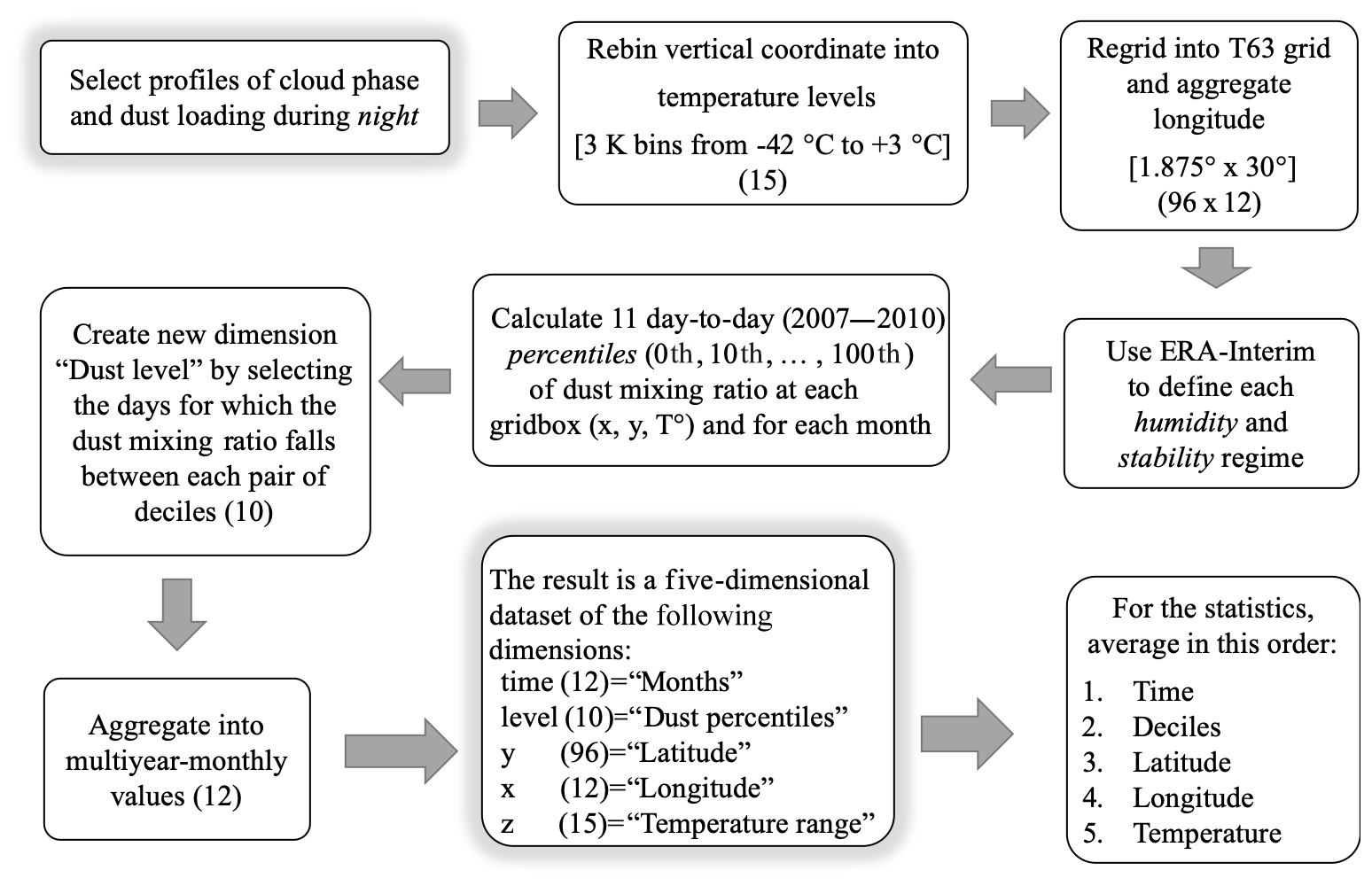
Figure 1Flow chart showing the processing steps starting from the raw data (satellite retrievals and model reanalysis) to the dataset used for the analysis.
In this section, the different processing steps of the datasets presented in Sect. 2 are described. Figure 1 presents a flow chart of this processing and a roadmap for the following subsections.
3.1 Selection of cloud profiles
In order to exclude the effects of the scattering of sunlight on the cloud-phase detection from the CALIOP lidar signal, only night-time retrievals were used. Including convective clouds – as retrieved by the 2B-CLDCLASS product (see Appendix) – does not introduce a significant bias on the results. This low sensitivity to convective clouds is mainly due to the low area fraction represented by such clouds, especially in the mixed-phase regime at the mid-latitudes (less than 5 %). Similarly, precipitating clouds had little impact on the results.
3.2 Regridding and rebinning: 3 K temperature levels and grid boxes
The cloud thermodynamic phase is mainly a function of temperature. Therefore, temperature bins of 3 K each were used as a vertical coordinate throughout the study to constrain the variability of cloud phase. For the MACC and ERA-Interim reanalyses, we rebin the model levels into 3 K intervals to match the vertical resolution of the CALIPSO-GOCCP product.
For each product, the latitude × longitude space was regridded using the nearest-neighbour method. We regridded the dataset first into a Gaussian T63 grid, then aggregated every 16 grid boxes along the longitude (; latitude longitude grid boxes) to better fill the horizontal gaps between the satellite orbits. The Gaussian T63 grid is commonly used in global climate models (GCMs) (Randall et al., 2007). It also facilitates comparisons with global simulations of cloud thermodynamic phase. In Sect. 4.4 and onwards, zonally averaged latitude bands of are used to allow for a direct comparison with previous studies (Zhang et al., 2018).
3.3 Meteorological regimes
Dust aerosol can produce or be accompanied by changes in atmospheric stability and humidity. To disentangle such effects, we constrain the cloud environment using the air relative humidity with respect to liquid and the tropospheric static stability. Depending on the isotherm to be studied, we use the lower troposphere static stability (LTSS) or the upper troposphere static stability (UTSS). These parameters are defined as
where Tx and Px are the temperature and pressure at the surface or at x hPa using the pressure levels of the ERA-Interim reanalysis. R is the gas constant and Cp the specific heat capacity of air (Klein and Hartmann, 1993). The static stability (see Eqs. 1 and 2) is defined as the difference in potential temperature between two pressure levels (Klein and Hartmann, 1993). It represents the gravitational resistance of an atmospheric column to vertical motions. Such vertical motions are traduced in a temperature change rate within the air parcel. Therefore, the static stability can have an important impact on the heterogeneous freezing rates, especially on immersion freezing. We note that the dynamic component of the atmospheric stability is not included in the static stability. Especially in the upper troposphere, atmospheric gravity waves occurring during stable thermal conditions may also result in vertical motions affecting ice production. The static stability and relative humidity are obtained from the ERA-Interim reanalysis.
3.4 Classification of dust loads and day-to-day correlation
In contrast to previous studies, in this work we want to isolate the day-to-day correlation between dust aerosol and cloud phase. In order to exclude the spatial component of the correlation, the complete time span 2007–2010 was used to assess the daily correlation between the MACC dust mixing ratio and the CALIPSO-GOCCP cloud phase. This correlation was done independently for each volume grid box – each constrained in latitude, longitude, and temperature.
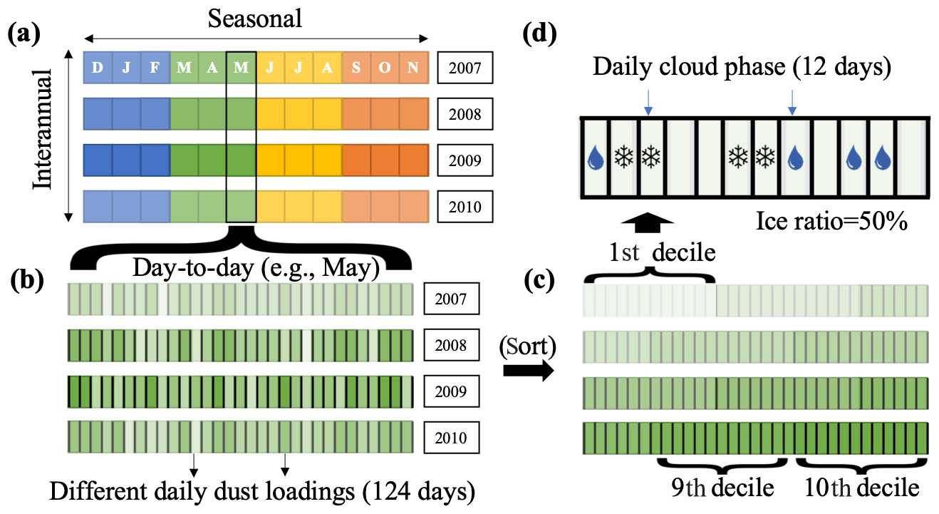
Figure 2Seasonal, day-to-day, and day-to-day decile concept as used in this study. For this example, the day-to-day analysis of May contains 124 daily datapoints. In step (a) to (b), only the daily values for one month of the year (May) are selected. In step (b) to (c), these daily values are sorted into 10 different deciles. In step (c) to (d), the average dust mixing ratio and ice frequency for each decile are calculated.
We also need to exclude the seasonal component of the temporal correlation. For this purpose, we process each month of the year independently. This is done as a multiyear selection (e.g. January containing January 2007, January 2008, January 2009, and January 2010) (see Fig. 2a–b).
The dust mixing ratio density distribution is heavily skewed to the right, while the cloud phase follows mostly a binary distribution. Because of this non-normality, a typical correlation approach like the Pearson's correlation coefficient will not reflect the genuine relationship between both variables (Hauke and Kossowski, 2011). Therefore, we use a rank correlation approach using the temporal quantiles of the dust loading. Specifically, we use the time deciles of the MACC dust mixing ratio to sort the daily values of cloud phase independently at each volume grid box. As a result, each cloud-phase value is associated with a specific daily dust rank: from exceptionally dust-free days (“1” for the lowest decile) to exceptionally dusty days (“10” for the highest decile). This step can be understood as sorting of the daily values (see Fig. 2b–c), where the neighbouring days are reordered and the timeline is lost. Finally, we average the daily values of dust loading and cloud phase inside each dust decile (see Fig. 2c–d).
The resulting field contains one extra dimension for each volume grid box (month, dust decile, temperature, latitude, longitude). Figure 2 presents a visualization of this process.
3.5 Data availability and averaging order
The day-to-day correlation approach relies strongly on the available sample size. For small sample sizes, only a few retrievals (daily means within a volume grid box) can be found for a given dust decile. In this case, the average FPR may still be non-normally distributed, introducing a larger standard deviation. Within a 12 K range, each zonally averaged latitude bin () contains about 1500 to 2000 observational datapoints in the mid-latitudes and about 500 to 1500 datapoints in the high latitudes. The smallest sample size was found for the southern high latitudes, where it drops down to about 400 at −15 ∘C, which corresponds to 7 % of the total possible sample size. In this case, many volume grid boxes contain only one retrieval for a given dust decile. Only after aggregating such grid boxes into a resolution will enough retrievals be averaged to obtain a normally distributed variable. Potential reasons for missing data are the following:
-
The satellite swaths (orbits) produce a different density of retrieved profiles at different latitudes.
-
Using only night-time data, the sample size in the meteorological summertime (shorter nights) is lower.
-
The cloud-phase retrievals are less frequent for seasons, regions, and heights with low cloud cover (see Fig. S8).
-
At high latitudes, relatively warm temperatures (e.g. −15 ∘C) exceeding the surface temperature can be found, and therefore no information is available for such temperatures (e.g. over Antarctica in winter).
The averaging order of the dimensions was defined – from first to last – as longitude, month, decile, latitude, and temperature. This choice prevents artefacts resulting from too many missing values. Latitude and temperature are averaged last because of the higher associated correlations with cloud phase (Sect. 4.2–4.3 of this study; Choi et al., 2010; Tan et al., 2014). Each grid of the newly defined grid boxes contains on average 100 to 200 datapoints at −15 ∘C (within a 12 K range) in the mid-latitudes. Meanwhile, in the subtropics and the high latitudes, the sample size is much more heterogeneously distributed. Near the poles and in subsidence regions, it can drop below 50 datapoints. A detailed view of the spatio-temporal distribution of the sample size for stratiform clouds can be found in the Supplement (Fig. S14).
In Sect. 4.1, the adjusted ice volume fraction,
is used instead of the traditional FPR, with cvf being the cloud volume fraction obtained from the GOCCP product. The adjusted FPR* helps to visualize the cloud thermodynamic phase of significant clouds – with high cvf – in the retrieval. This alternative is only used in the case study to aid the visualization of the cloud ice and liquid.

Figure 3Sample size of cloud phase (CALIPSO-GOCCP) of each latitude band for −15 ∘C (range −21 to 9 ∘C) and −30 ∘C (range −36 to −24 ∘C) for the period 2007–2010. Each count corresponds to a grid box in a 3 K temperature bin at a specific month of the year and inside a specific dust decile. The theoretical maximal sample size for each latitude band is 5760 for a 12 K temperature range.
4.1 Case study
This section seeks a better understanding of the ice-to-liquid ratio retrieved in the CALIPSO-GOCCP product. We provide a detailed case study of a stratiform cloud scenario. In this scenario, four stratiform cloud types from the CloudSat classification are included: stratocumulus (low-level clouds), altostratus and altocumulus (mid-level clouds), and cirrus (high-level clouds). Although not present in the case study, nimbostratus are included in the analysis of cloud phase as well and are particularly important in the high latitudes. Stratus clouds are defined for temperatures above 0 ∘C; therefore, they are not relevant for this study. Finally, the horizontal extension of cumulus and deep-convective clouds is very low compared to the stratiform clouds and can be therefore ignored in our study, especially outside the tropics (Sassen and Wang, 2008).
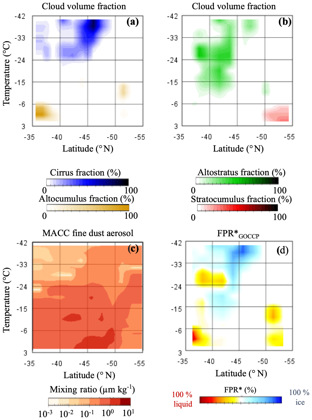
Figure 4Case study 09:50 UTC 14 December 2010 for temperatures between −42 and +3 ∘C. (a–b) Cloud volume fraction (GOCCP) for different cloud types (CloudSat cloud classification). (c) Fine dust (0.03–0.55 µm) aerosol mixing ratio (MACC reanalysis); note the logarithmic scale. (d) Adjusted ice occurrence frequency derived from the CALIPSO-GOCCP product. FPR*: frequency phase ratio (ice voxels divided by total voxels; see Eq. 3). White colours represent clear sky. The fields were co-located in a grid with temperature bins of 3 K each.
The A-Train segment shown in Fig. 4 has been already chosen for a previous case study (Huang et al., 2015) due to the variety of cloud types it contains. For this segment, we separate the clouds classified as cirrus and altocumulus (Fig. 4a). Similarly, we can also separate altostratus and stratocumulus (Fig. 4b). These four cloud types are frequently thin enough to be penetrated by lidar and radar systems. Therefore they are an excellent target to study cloud glaciation processes (Bühl et al., 2016; Zhang et al., 2010). Stratiform clouds are simpler to study than convective clouds, because they are affected by weaker updraughts and the microphysical evolution (i.e. ice formation) is less affected by secondary and ice multiplication effects (Westbrook and Illingworth, 2011). Figure 4c shows the mixing ratio of fine (0.03–0.55 µm) dust aerosol (MACC reanalysis) for the same vertical plane. As in this case study, the dust loading can vary within several orders of magnitude on the synoptical scale. On the same scale, we can usually observe clouds with different cloud phases (Fig. 4d). Therefore, combining many cases, it is possible to assess both the spatial and temporal correlation between both variables. This assessment may shed some light on the potential role of dust aerosol as a driver of cloud glaciation in stratiform clouds.
4.2 Temperature dependence
Temperature is the main factor controlling the thermodynamic phase of clouds. Mixed-phase clouds between 0 and −25 ∘C are usually topped by a liquid layer (Ansmann et al., 2008; De Boer et al., 2011; Westbrook and Illingworth, 2011). Below this layer, there is often a thicker layer containing ice particles. The CALIOP backscatter signal is usually already strongly attenuated at such depths and often cannot detect large ice particles. Therefore, the CALIPSO-GOCCP algorithm usually classifies the whole cloud layer as liquid (Huang et al., 2012, 2015).
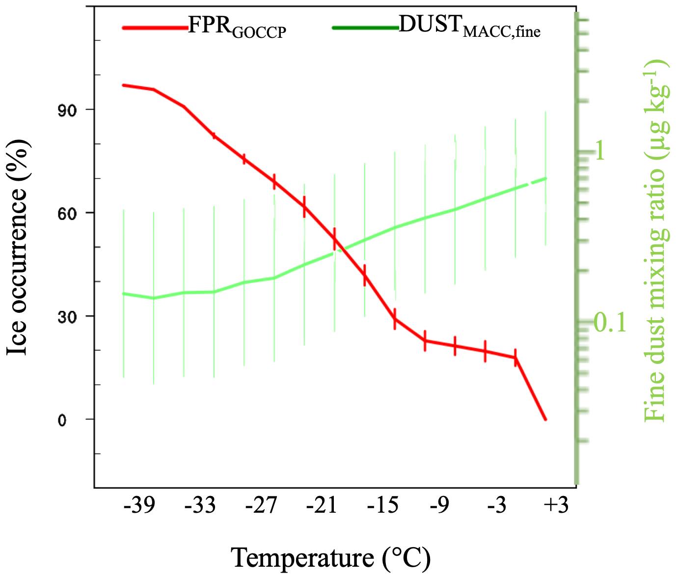
Figure 5Global ice cloud occurrence frequency (2007–2010). The fine-mode dust mixing ratio from the MACC reanalysis corresponds to the range 0.03–0.55 µm and is presented on a logarithmic scale on the right vertical axis. Each temperature bin spans 3 K. The vertical bars show the mean day-to-day standard deviation between different fine-mode dust deciles.
Figure 5 shows that the global average FPR as a function of temperature decreases roughly from 100 % at −40.5 ∘C via about 20 % at −1.5 ∘C and down to 0 % at +1.5 ∘C. This temperature dependence between −42 ∘C and 0 ∘C is also observed for a wide range of parameterizations in global climate models (Cesana et al., 2015). This pattern can also be found in ground-based measurements (Kanitz et al., 2011), spaceborne lidar measurements (Tan et al., 2014), and aircraft measurements (McCoy et al., 2016).
Additionally, the average fine-mode dust mixing ratio is also shown in Fig. 5. At the height of the 0 ∘C isotherm, the mixing ratio is on average higher than at the −42 ∘C isotherm (note the logarithmic right y axis). This reflects the fact that, on average, dust mixing ratios tend to be higher near the dust sources at the surface. However, this does not imply any general relationship between dust and temperature. Moreover, instant vertical profiles of dust loading and temperature may differ greatly from this average, especially in the long-range transport of dust plumes.
4.3 Latitude dependence
For both temperature ranges shown in Fig. 6 the absolute maximum of FPR is located near the Equator (85 % at −30 ∘C and 44 % at −15 ∘C). These maxima are probably associated with the enhanced homogeneous freezing in the tropics at temperatures below −40 ∘C and the resulting downward transport of cloud ice – also known as ice detrainment. Similarly, the minima are observed towards the high latitudes. At −30 ∘C, the FPR has two local maxima with values of 76 % and 84 % near 39∘ S and 39∘ N, respectively. At −30 ∘C, the FPR is higher in the Northern Hemisphere than in the Southern Hemisphere, in particular for the high latitudes. This higher FPR coincides with the higher average dust mixing ratio in the Northern Hemisphere. Such positive spatial correlations between FPR and dust aerosol have been already pointed out using the dust occurrence frequency derived from CALIOP (Choi et al., 2010; Tan et al., 2014; Zhang et al., 2012).
At −15 ∘C, in the southern high latitudes a local minimum in FPR near 73∘ S is followed by a steep increase at 84∘ S. The larger standard deviation in these latitudes is possibly a result of the low sample size in the region (as mentioned in Sect. 3). However, the higher FPR in the southern than in the northern polar region is consistent with the fraction of ice clouds reported previously in the literature at −20 ∘C (Li et al., 2017a). On the other hand, it has been shown that the orographic forcing in Antarctica can lead to high ice water contents for maritime air intrusions (Scott and Lubin, 2016). In other words, maritime air intrusions associated with higher temperatures, higher concentrations of INPs, and stronger vertical motions could explain the observed pattern in the southern polar regions. However, the low sample size near the South Pole (Figs. 3 and S14b) and the low altitude of the −15 ∘C isotherm (Fig. S12b) result in a lower confidence in the results for this region. For example, at −15 ∘C, the zonal standard deviation of the FPR significantly increases from 60∘S towards the South Pole – from about ±0.08 to ±0.16 in Fig. 6a – at the same time that the sample size decreases from 2200 to 300 (Fig. 3).
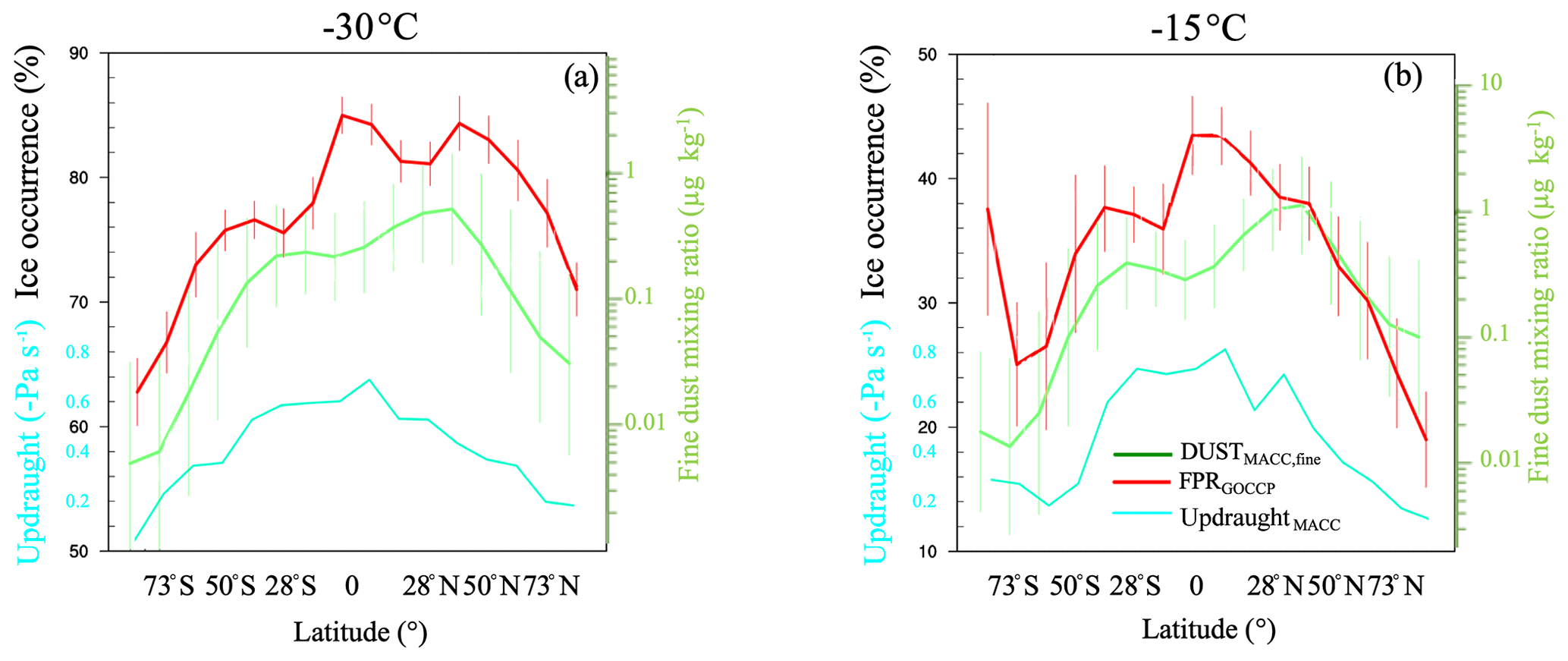
Figure 6Zonal mean of stratiform cloud ice occurrence frequency for (a) −30 ∘C (range −36 to −24 ∘C) and (b) −15 ∘C (range −21 to −9 ∘C) averaged over the period 2007–2010. Each datapoint corresponds to a zonal band of 11.25∘ width. The average fine-mode dust mixing ratio of each band is also shown on the right vertical axis (note the logarithmic scale). The average large-scale vertical velocity (updraught) from the MACC reanalysis is also shown (cyan axis on the left of each plot). The vertical bars show the mean day-to-day standard deviation between different fine-mode dust deciles. The curves for dust and updraught are slightly shifted left and right, respectively, to fit all vertical bars.
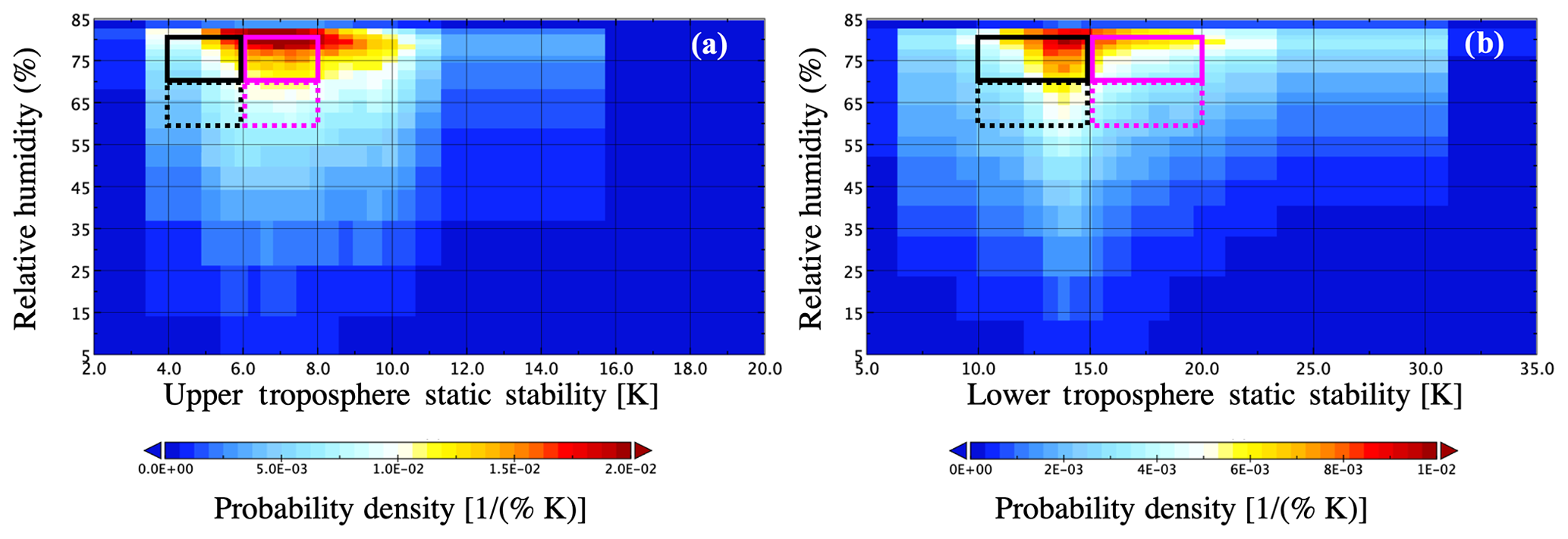
Figure 7Probability histogram at −22 ∘C (range −27 to −18 ∘C) for 2007 for different conditions of relative humidity against (a) upper troposphere static stability and (b) lower troposphere static stability. All-sky grid boxes are included for the entire globe. The values for relative humidity are taken from the ERA-Interim dataset, and the static stability is calculated from the ERA-Interim pressure levels. The magenta and black boxes represent the regimes used in the study.
For the clouds studied, the time-averaged large-scale vertical velocity (from the MACC reanalysis, shown in Fig. 6) is regionally correlated with the FPR at −15 ∘C. The Pearson correlation coefficient was 0.47 using zonal averages and 0.31 using the grid box averages. Moreover, in another study, the spatial correlation between large-scale updraught velocity at 500 hPa was also found to be positively correlated (spatially) to the occurrence frequency of ice clouds at −20 ∘C (Li et al., 2017a). In other words, both the dust mixing ratio and the large-scale vertical velocity appear to be to some extent correlated (spatially) to the FPR. There are some plausible explanations for this correlation:
-
The spatial correlation can be a result of an enhanced transport of water vapour to higher levels at temperatures below −40 ∘C and the subsequent sedimentation of ice crystals from the homogeneous regime (Convective detrainment of ice).
-
The updraughts are associated with higher availability of INPs at the cloud level (from below the cloud), and the effect is large enough to mask the enhanced droplet growth typically associated with updraughts.
-
The updraughts enhance a certain type of heterogeneous nucleation requiring saturation over liquid water (e.g. immersion freezing). Updraughts generate a local adiabatic cooling, possibly activating INPs that may not have been active before at higher temperatures.
To the authors' knowledge, there is currently no observational constraint to the source of cloud ice in the mixed-phase regime. Namely, the frequency of ice clouds between 0 and −42 ∘C may be dominated by either convective ice detrainment or by in situ freezing of cloud droplets. Overall, the relative contribution of heterogeneous and homogeneous freezing – and the different INP types – is still a matter of debate (Dietlicher et al., 2019; Barahona et al., 2017; Sullivan et al., 2016).
4.4 Constraining the influence of static stability and humidity on the dust–cloud-phase relationship
In the following sections, the temporal correlation between mineral dust mixing ratio and cloud ice occurrence frequency is referred to as the dust–cloud-phase relationship. To study this relationship, we classify the retrievals into different weather regimes to constrain the meteorological influence. The resulting dust–cloud-phase relationship for different regimes may offer a good insight into the processes underlying the dust–cloud-phase relationship. Particularly, how heterogeneous freezing by dust aerosol may affect the cloud thermodynamic phase on a day-to-day timescale.
In other words, to extract the specific influence of mineral dust on cloud glaciation, it is necessary to identify and constrain relevant meteorological confounding factors (Gryspeerdt et al., 2016). The atmospheric relative humidity and static stability are good candidates for such a confounding factor (Zamora et al., 2018). Both are correlated with the transport of mineral dust and vary between different cloud regimes. Additionally, relative humidity is, next to the temperature, one of the main factors in the initiation of ice nucleation in laboratory studies (Hoose and Möhler, 2012; Welti et al., 2009).
The effect of humidity and static stability on ice production is not straightforward. In general, moist and unstable conditions are associated with enhanced lifting of air that likely causes nucleation of hydrometeors. Between 0 and −40 ∘C, the supersaturation of water vapour over liquid enhances the liquid formation. However, the depositional growth of ice is rather inefficient within strong updraughts (Korolev et al., 2017). At temperatures below −40 ∘C, the ice production due to deposition and homogeneous nucleation dominate. The ice particles aloft can result in a higher occurrence of cloud ice in the mixed-phase regime below due to ice sedimentation. To constrain both the atmospheric stability and humidity, a subset of the data must be found within a narrow range of these variables. At the same time, enough datapoints must still be available to assess the dust–cloud-phase relationship. For this purpose, we use a probability histogram to define the regime bounds such that at least 10 % of the data is included in each regime (see Fig. 7).
For the relative humidity, the bounds are defined at 60, 70, and 80 %; for the LTSS, they are defined at 10, 15, and 20 K; and for the UTSS, they are at 4, 6, and 8 K. The fraction of data inside each regime corresponds to the integral of the probability density within the regime bounds. For example, if the probability density between 4–6 K and 70 %–80 % is 0.01, then 20 % of the data is contained between these bounds. The magenta boxes in Fig. 7 represent the different stability and humidity regimes used for the lower and upper troposphere.

Figure 8Average cloud phase (GOCCP) for the mid-latitude and high-latitude bands averaged between −21 and −9 ∘C in the period 2007–2010 for different regimes of relative humidity (a, c low RH; b, c high RH) and lower tropospheric static stability (a, b high LTSS; c, d low LTSS). The horizontal axis corresponds to the different time deciles (day-to-day variability) of fine-mode dust mixing ratio (MACC) calculated for each 3 K temperature bin and grid box () and averaged along each 12 K temperature range and latitude band. The vertical bars are positioned at each dust decile and show the mean zonal standard deviation within each latitude band.
For dust mixing ratios between 0.1 and 2.0 µg kg−1 at −15 ∘C, the dust–cloud-phase curve in both mid-latitudes follows a similar logarithmic increase in cloud ice occurrence frequency of about +6 % for low-LTSS and +4 % for high LTSS conditions (see Fig. 8). After analysing 11 years of ground-based lidar measurements in Leipzig, Seifert et al. (2010) reported a slightly higher increase by about +10 % between −10 and −20 ∘C for dust concentrations between 0.001 and 2 µg m−3 (note the different units). In our results at −15 ∘C, the cloud ice occurrence frequency tends to be higher for higher relative humidity, and the LTSS seems to have a major effect on the dust–cloud-phase relationship. For high-LTSS conditions (Fig. 8a–b), a positive dust–cloud-phase correlation can be observed at all four latitude bands. The slope is similar for the Northern Hemisphere and Southern Hemisphere latitudes and for the middle and high latitudes.
At high LTSS in the high latitudes, the range of ice occurrence frequency values is higher than for the mid-latitudes and small increases in dust mixing ratio are associated with a strong increase in cloud ice occurrence frequency. For the high-LTSS regime, the ice occurrence frequency in the southern high latitudes increases by +8 %. In contrast, at mid-latitudes the increase is only about +4 %. In both middle and high latitudes, the cloud ice occurrence frequency for the same dust mixing ratio is about +2 % to +8 % higher in the Southern Hemisphere than in the Northern Hemisphere. This contrast could point to a factor – other than dust aerosol – causing an increased ice occurrence frequency in the Southern Hemisphere. The contrast could also suggest a potential difference in the sensitivity of cloud glaciation to mineral dust between hemispheres. In the high-RH regime, the difference between Northern Hemisphere and Southern Hemisphere is reduced, as well as the standard deviation of the FPR. This reduction may be due to the higher sample size density in the high-RH regime. For the low-LTSS regime (Fig. 8c–d), the cloud thermodynamic phase in the high latitudes remains mostly constant for increasing dust mixing ratios. For the same regime, the maximum FPR in the southern mid-latitudes is similar to the minimum in the northern mid-latitudes. This agreement suggests a more consistent sensitivity of cloud glaciation to mineral dust for unstable conditions.
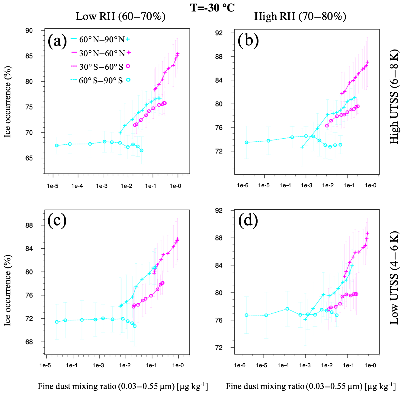
Figure 9Same as Fig. 8 but averaged from −36 to −24 ∘C and using the upper tropospheric static stability (UTSS).
At −30 ∘C, the cloud ice occurrence frequency in the southern high latitudes remains almost constant for increasing dust mixing ratios (see Fig. 9). For the high-RH regime, the cloud ice occurrence frequency tends to be higher than in the low-RH regime. This difference is evident for the southern high latitudes for which the cloud ice occurrence frequency is about +4 % higher in the high-RH regime. For dust mixing ratios between 0.1 and 1.5 µg kg−1, the cloud ice occurrence frequency at −30 ∘C increases by about +5 %. The highest increase is found for the northern latitudes. However, the results from the southern mid-latitudes contradict the notion that the INP activity of mineral dust is of secondary importance in the Southern Hemisphere due to low dust aerosol concentrations (Burrows et al., 2013; Kanitz et al., 2011). Nevertheless, recent studies have acknowledged that the importance of mineral dust in southern latitudes still cannot be ruled out (Vergara-Temprado et al., 2017).
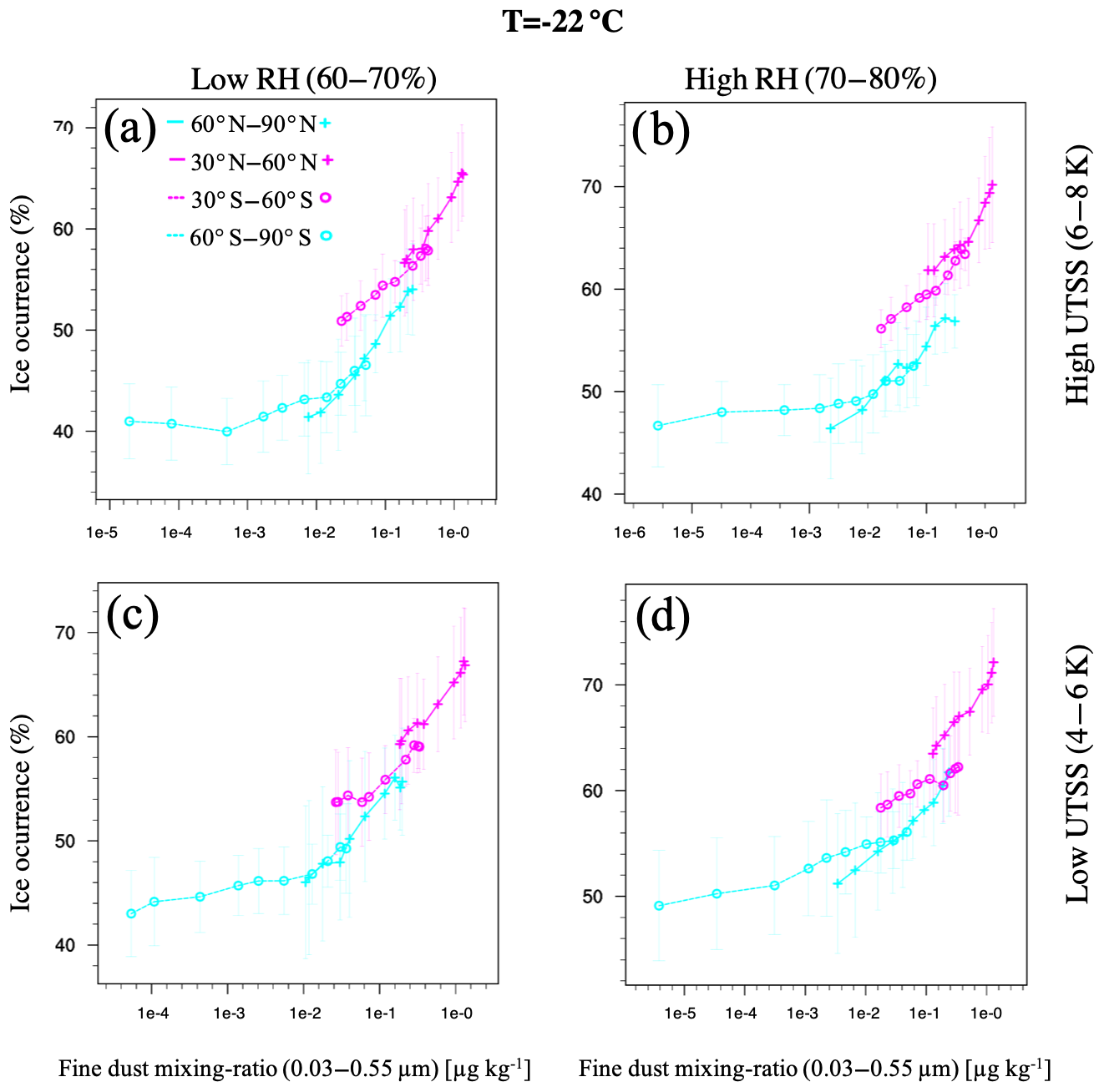
At −22 ∘C, the cloud ice occurrence frequency is higher in the high-RH regime (Fig. 10), similar to the results at −15 and −30 ∘C. For high-UTSS conditions, the dust–cloud-phase curves are in closer agreement between the Northern Hemisphere and Southern Hemisphere. This coincidence suggests a similar sensitivity of cloud glaciation to mineral dust for both hemispheres. For mixing ratios between 0.01 and 1.0 µg kg−1 at −22 ∘C, the ice occurrence frequency increases by about 25 % at high-UTSS conditions and by about 20 % at low-UTSS conditions. From the three temperature regimes studied, at −22 ∘C the four latitude bands show the best agreement between Northern Hemisphere and Southern Hemisphere and also between middle and high latitudes. With these results, the dust–cloud-phase correlation may help clarify not only the day-to-day differences in cloud glaciation but also the differences between latitudes.
At all temperatures studied, higher humidity values were associated with a higher cloud ice occurrence frequency. Additionally, for similar dust loadings, the cloud ice occurrence frequency was found to be higher at the mid-latitudes than at the high latitudes. However, against our expectations, for similar dust loadings the cloud ice occurrence frequency at −15 ∘C was higher in the Southern Hemisphere than in the Northern Hemisphere.
Some studies have already suggested that the lower occurrence frequency of cloud ice in the higher latitudes may be associated with lower INP concentrations (Li et al., 2017a; Tan et al., 2014; Zhang et al., 2012). This hypothesis has been supported mainly by the spatial correlation between the dust relative aerosol frequency and the occurrence frequency of ice clouds retrieved from satellite observations. However, evidence of the day-to-day co-variability between INPs and cloud ice was lacking up to now. Furthermore, by studying the dust–cloud-phase relationship it is possible to extract new information about the differences in cloud glaciation at different latitudes and to connect these differences to previous studies of heterogeneous freezing. Particularly, our results may be used to evaluate our current knowledge of the global differences in the mineralogy of dust aerosol and its freezing efficiency.
5.1 North–south contrast
We have found that the ice occurrence frequency can vary at different latitudes even for similar mixing ratios of mineral dust. This variability could be explained by differences in the mineralogical composition of the mineral dust aerosol at the Southern Hemisphere and Northern Hemisphere. Clay minerals from the Northern Hemisphere are composed mostly of illite and smectite (Claquin et al., 1999). It has been suggested that the freezing efficiency of these minerals can be well represented by the mineral montmorillonite (Hoose et al., 2008). In contrast, the Southern Hemisphere clay minerals are better represented by the mineral kaolinite (Claquin et al., 1999; Hoose et al., 2008), which is less efficient in the immersion mode. The freezing efficiencies of kaolinite and montmorillonite are known for both the immersion and contact freezing modes (Diehl et al., 2006; Diehl and Wurzler, 2004). Following this assumption, the immersion freezing rates at −30 ∘C would be about 300 times higher in the Northern Hemisphere than in the Southern Hemisphere. This difference could explain the higher ice occurrence frequency in the Northern Hemisphere relative to the Southern Hemisphere for similar dust mixing ratios at −30 ∘C.
For temperatures higher than −25 ∘C, contact freezing starts to dominate over immersion freezing. However, between −25 and −16 ∘C the contact freezing efficiency is similar for kaolinite and montmorillonite. This balance may explain why the ice occurrence frequency in the Northern Hemisphere is only slightly higher for similar dust mixing ratios at −22 ∘C. Finally, between −15 and −4 ∘C, the contact freezing efficiency of montmorillonite is again higher than for kaolinite. However, this returned contrast fails to explain the higher ice occurrence frequency found in the Southern Hemisphere at −15 ∘C.
Nevertheless, at such high temperatures, other dust minerals like feldspar mineral are much more efficient as ice-nucleating particles than clay minerals (Atkinson et al., 2013). Moreover, it could be that the effect of such feldspar minerals dominates over the effect of clay minerals at high temperatures. Indeed, such efficient minerals are believed to deplete quickly trough heterogeneous freezing. Therefore, only a few of these aerosols would reach lower temperatures. Thus, they are likely more relevant at temperatures above −20 ∘C, where the immersion efficiency of clay minerals quickly decays (Boose et al., 2016; Broadley et al., 2012; Murray et al., 2011).
If feldspar minerals do dominate the heterogeneous freezing due to mineral dust above −20 ∘C, then the higher cloud ice occurrence frequency in the Southern Hemisphere may be due to a higher fraction (or higher efficiency) of feldspar minerals in the southern dust particles. Some evidence for this has been already found by comparing the immersion freezing efficiency of dust particles from different deserts worldwide (Boose et al., 2016). In these results, the immersion efficiency of dust particles lays mostly between kaolinite and K-feldspar. The dust samples from sources in the Southern Hemisphere (Australia, Etosha, and Atacama milled) have a higher freezing efficiency than most of the samples from the Northern Hemisphere sources including Saharan sources for temperatures below −24 ∘C. Unfortunately, only four of these samples were studied for higher temperatures, between −23 and −11 ∘C. However, it was again a sample from the Southern Hemisphere (Atacama milled), which exhibited the highest freezing efficiency. We may assume that the higher freezing efficiency of the southern dust sources can be extrapolated to temperatures above −20 ∘C. Then, at −15 ∘C the higher immersion efficiency of southern mineral dust, possibly due to higher feldspar fractions, may explain the higher ice occurrence frequency in the Southern Hemisphere. The highly efficient particles, most likely feldspar minerals, would be quickly depleted at temperatures around −15 ∘C and would therefore not interfere with the kaolinite–illite (montmorillonite) differences at −30 ∘C.
Table 1Summary of the north–south differences in the cloud phase associated with mineral dust based on the day-to-day statistics for the middle and high latitudes.
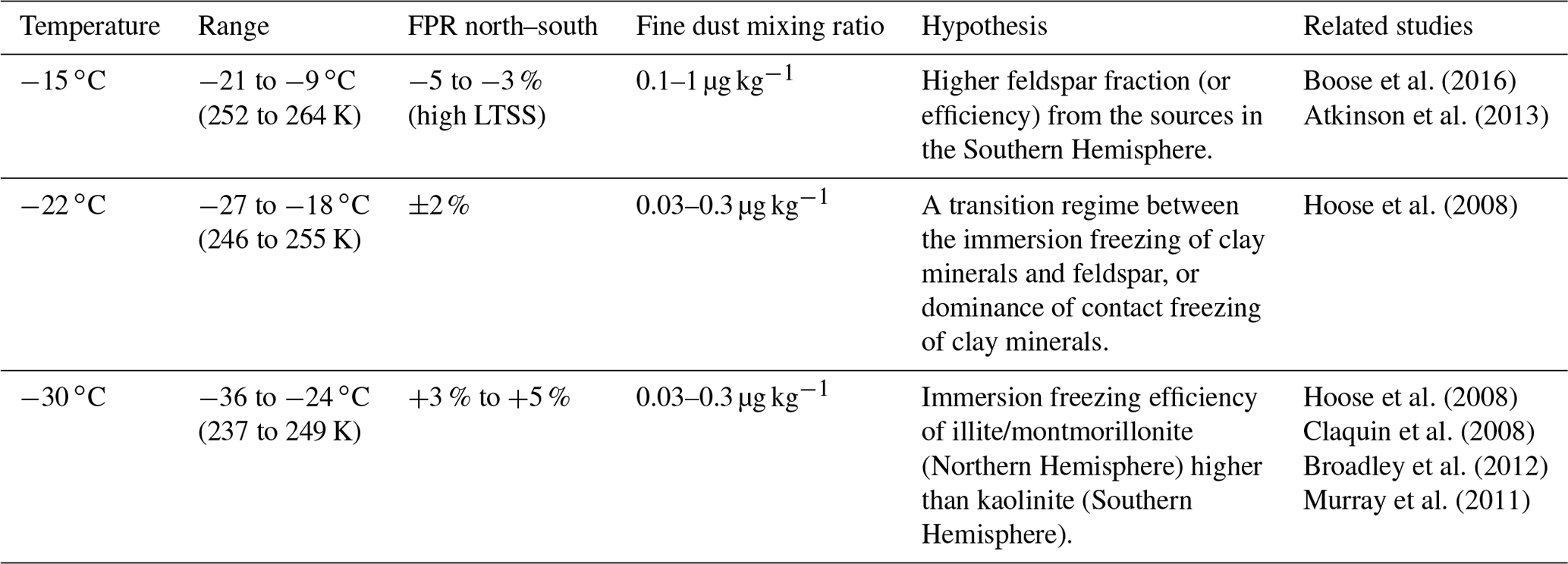
Furthermore, such a depletion of highly efficient INPs during the transport of dust aerosol may also explain the higher ice occurrence frequency at the mid-latitudes compared to the high latitudes for similar mixing ratios of mineral dust, especially at higher temperatures. The ageing (e.g. internal mixing with sulfate or “coating”) of dust particles may also reduce the freezing efficiency of dust aerosol during the transport from low to high latitudes. The hypotheses explaining the differences in the freezing behaviour of dust between the Northern Hemisphere and Southern Hemisphere are summarized in Table .
5.2 Assumptions and uncertainties
In the analysis presented above, certain assumptions were made to assess the potential effect of mineral dust on cloud thermodynamic phase. In this section, these assumptions and the uncertainties that arise from them, as well as the subsequent limitations of the resulting interpretation, will be discussed.
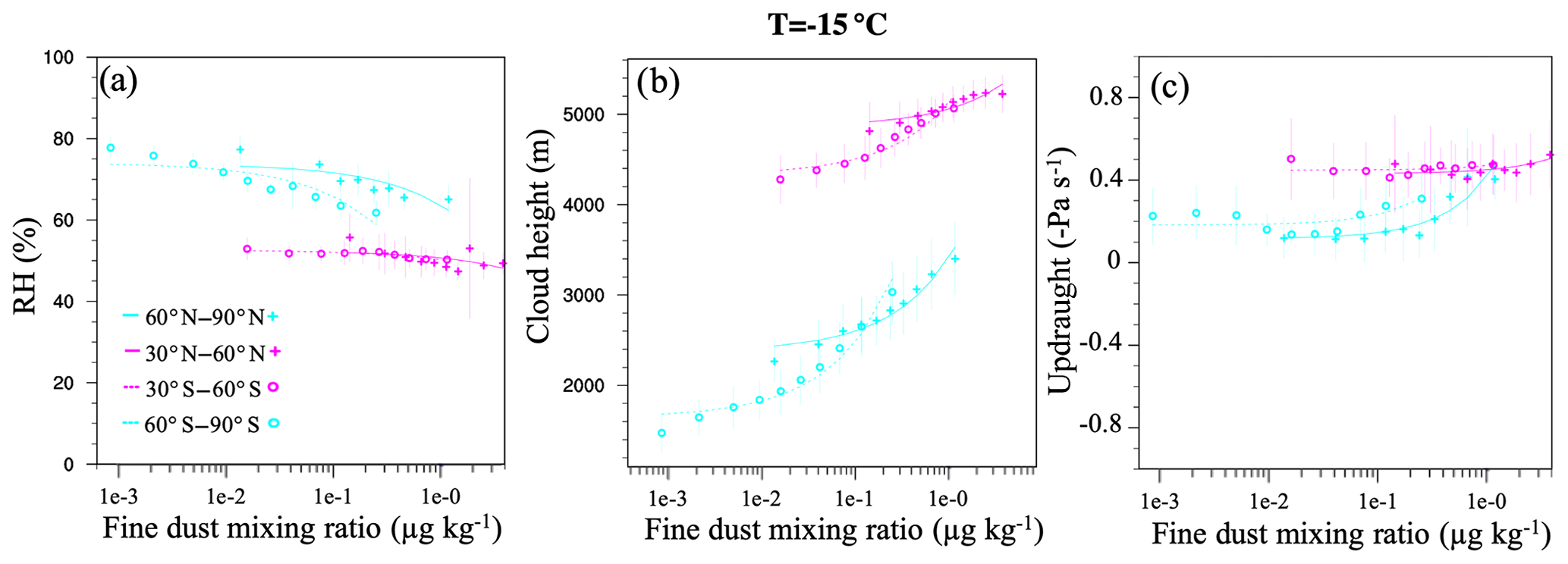
Figure 11Same as Fig. 8 but for (a) ERA-Interim relative humidity, (b) ECMWF-AUX isotherm height, and (c) MACC large-scale vertical velocity at −15 ∘C. The average of each variable is weighted by cloud volume fraction.
Concerning the vertical resolutions of the different products, the choice of 3 K bins is based on the original 3 K bins of the CALIPSO-GOCCP product. Using a coarser vertical resolution (e.g. 6 K bins) would hinder the assessment of the role of dust as INPs. For example, a decrease of 3 K in temperature is roughly equivalent to a 5-fold increase in INP concentrations (e.g. Niemand et al., 2012). At the middle and high latitudes, the typical standard deviation of the day-to-day dust mixing ratio corresponds to roughly a 4-fold increase from the mean (see Fig. S5); therefore, we expect that the variability of dust loading should dominate over temperature variations, given a temperature constraint of about 3 K or less.
As mentioned in Sect. 3, we excluded the seasonal component of the dust–cloud-phase correlation by calculating the deciles independently for each month of the year. However, shorter cycles (e.g. weather variability) may still influence the variability of dust and cloud phase. For example, below the −42 ∘C isotherm more liquid clouds are found in convective sectors and more cirrus clouds at the detrainment regions. However, it is still possible to distinguish between dusty and non-dusty conditions at each point of the weather cycle. Consequently, once we average over the weather cycle – using monthly means inside each dust percentile – we expect the dust–cloud-phase relationship to be dominated by the microphysical effect of dust on cloud phase.
Despite the long period (2007–2010) used in the study, a significant fraction of the five-dimensional space used for our analysis (10 dust deciles, 12 months, 15 temperature bins, 96 latitudes, and 12 longitudes) is sparsely sampled or even contains missing values. In the high latitudes, a sampling bias exists towards the respective winter seasons, because very few night-time retrievals are available in summer. However, the seasonal variability was not found to be a dominating factor in the day-to-day impact of dust mixing ratio on the FPR (see Fig. S19). Furthermore, many factors may contribute to higher standard deviations for the ice occurrence, including
-
changes in dynamical forcing (e.g. updraughts) and cloud regimes;
-
temperature changes after cloud glaciation (e.g. latent heat release);
-
ice sedimentation from above (cloud seeding) and INPs other than dust;
-
cloud vertical distribution within the studied temperature ranges;
-
turbulence favouring aerosol mixing and sub-grid temperature fluctuations;
-
differences in dust mineral composition, electric charge, or size;
-
coatings (e.g. sulfate) affecting aerosol solubility and freezing efficiency;
-
subsetting of the data (e.g. only night-time retrievals).
Additionally, some issues arise from the coarse spatial resolution used in our study. A high dust mixing ratio simulated in a volume grid box indicated as cloudy by the satellite observations does not ensure that the dust is actually mixed with the cloud. The sub-grid distribution of dust relative to the exact cloud position remains unresolved. Higher dust mixing ratios should be interpreted as an indicator or a higher probability that a significant amount of dust was mixed with a co-located cloud. This mixing may have happened during or before the observation by the satellite. However, we can assume that both cloud and dust aerosol followed a similar trajectory up to the moment of the observation. Overall, at coarse resolutions, the combination of modelled dust concentrations with satellite-retrieved cloud properties cannot guarantee the mixture of aerosol and clouds (Li et al., 2017b). Similarly, the atmospheric parameters obtained from the reanalysis may not match the conditions for the exact position of the clouds in the satellite retrievals. However, the atmospheric parameters are expected to match on average the large-scale conditions influencing the aerosol–cloud interactions.
As mentioned in Sect. 3, the total aerosol optical depth (AOD) from MODIS is assimilated in the MACC reanalysis. In general, we expect this assimilation to produce a fair estimation of the large-scale aerosol conditions on a day-to-day basis. At least for the Northern Hemisphere, this has been already validated with in situ measurements (Cuevas et al., 2015). Both the ERA-Interim and the MACC reanalysis are based on the IFS. Thus, both the aerosol and meteorological estimations are consistent.
The CALIPSO-GOCCP product relies on CALIOP to determine the presence of clouds. Nevertheless, the reader should be aware that several uncertainties remain. For example, the meteorology in the reanalysis and in the real atmosphere may differ, particularly on the sub-grid scale. In the worst case that the reanalyses are entirely inconsistent with the retrievals of cloud phase, we expect that the result would be the lack of correlation between dust and the ice occurrence (Figs. 8–10). We have included a reasonably large dataset for the study. Certainly, mismatches between reanalysis and cloud retrievals are possible. However, these would cause an underestimation – and not an overestimation – of the dust–cloud-phase correlation.
Concerning the interpretation of our results, it cannot be ruled out that the increase in ice cloud occurrence in the Southern Hemisphere for higher dust loading arises from other types of INPs such as biogenic aerosol (Burrows et al., 2013; O'Sullivan et al., 2018; Petters and Wright, 2015) or background free-tropospheric aerosol (Lacher et al., 2018), which could be misclassified as mineral dust in the reanalysis. Similarly, a possible correlation between ice cloud occurrence and the atmospheric conditions leading to the emission and transport of mineral dust should be further investigated (e.g. dusty air masses from land are usually warmer and drier). Another interesting explanation of the results presented in this study could involve the mixing of mineral dust particles with ice nucleation active macromolecules (Augustin-Bauditz et al., 2016). Such particles are in the size range of a few 10 nm (Fröhlich-Nowoisky et al., 2015) and would therefore not be detected if mixed with dust aerosol. Furthermore, biases such as the overestimation of the fine-mode dust aerosol in the MACC reanalysis (Ansmann et al., 2017; Kok, 2011) may shift the mixing ratios shown in Sect. 4.4. However, as long as such biases are not limited to certain meteorological conditions, the cloud phase averaged inside each dust decile should remain unaffected.
In general, meteorological parameters have a larger impact on cloud properties than aerosols do (Gryspeerdt et al., 2016). For example, different updraught regimes can change the aerosol–cloud interactions in warm clouds by an order of magnitude. Therefore, it is essential to study how such meteorological parameters relate to the dust aerosol loading. Firstly, the correlation between fine-mode dust mixing ratio and the RH from the ERA-Interim reanalysis – weighted by cloud volume fraction – was found to be negative (see Fig. 11a). We note that the RH from ERA-Interim represents the conditions at a large scale and not the conditions at a specific location or the moment of the interaction between dust aerosol and supercooled cloud droplets. Still, this relationship is consistent with the intuition that dust is mostly associated with drier air masses.
Second, the significant positive correlation found between dust aerosol mixing ratio and the height of the isotherms (weighted by cloud volume fraction) points to a possible source of uncertainty (Fig. 11b). This correlation could be due to clouds being detected in a higher temperature bin after being glaciated at lower temperatures. Thus erroneously suggesting an enhanced glaciation occurrence frequency at higher temperatures. Therefore, future studies must take into account this possibility when studying the occurrence of ice clouds at a certain isotherm. More details on the spatio-temporal variability of the cloud height can be found in the Supplement (Fig. S12). Lastly, Fig. 11c shows a positive correlation between the fine-mode dust and the large-scale vertical velocity from the MACC reanalysis at −15 ∘C. Updraughts favour saturation over liquid water and therefore cloud condensation nuclei (CCN) activation, droplet growth, and inhibition of the Wegener–Bergeron–Findeisen process. Therefore, a positive dust–updraught correlation could lead to an underestimation of the dust–cloud-phase relationship.
In summary, much of the co-variability between dust, humidity, updraughts, temperature, and cloud ice occurrence frequency is still poorly understood. However, we expect that the constrains on humidity and static stability minimized most of the biases discussed in this section.
For the first time, an aerosol reanalysis was combined with satellite retrievals of cloud thermodynamic phase to investigate the potential effect of mineral dust as INPs on cloud glaciation. We studied this effect on a day-to-day basis at a global scale for the period 2007–2010 focusing on stratiform clouds observed at night-time in the middle and high latitudes. Our main findings can be summarized as follows:
-
Between −36 and −9 ∘C, day-to-day increases in fine-mode dust mixing ratio (from lowest to highest decile) were mostly associated with increases in the day-to-day cloud ice occurrence frequency (FPR) of about 5 % to 10 % in the middle and high latitudes.
-
The response of cloud ice occurrence frequency to variations in the fine-mode dust mixing ratio was similar between the middle and high latitudes and between the Southern Hemisphere and Northern Hemisphere. Even though dust aerosol is believed to play a minor role in cloud glaciation in the Antarctic region, increases in FPR from first to last dust decile were also present in both the northern and southern high latitudes.
-
Using constraints on atmospheric humidity and static stability we could partly remove the confounding effects due to meteorological changes associated with dust aerosol.
-
The results also suggest the existence of different sensitivities to mineral dust for different latitude bands. The north–south differences in ice occurrence frequency for similar mineral dust mixing ratios agree with previous studies on the mineralogical differences between the Southern Hemisphere and Northern Hemisphere. A larger fraction of feldspar in the Southern Hemisphere could explain the differences at −15 ∘C, and the higher freezing efficiency of illite and smectite (more abundant in the Northern Hemisphere) over kaolinite (more abundant in the Southern Hemisphere) could explain the differences at −30 ∘C.
We believe these new findings may have an important influence on improving the understanding of heterogeneous freezing and the indirect radiative impact of aerosol–cloud interactions. The authors hope that the results of this work will also motivate further research, including field campaigns in remote regions, to study the day-to-day variability of cloud thermodynamic phase and the role of mineral dust in ice formation, satellite-based studies of associated changes in the radiative fluxes, and modelling studies to test the representation and relevance of specific processes involved in ice formation and mineral dust transport. Such studies could help to further improve our understanding of the influence of mineral dust or other aerosol types on cloud glaciation and the climate system.
Although in our study we used the cloud-phase classification from the CALIPSO-GOCCP product, other products are also available. Therefore, we include in the following appendix a detailed comparison between the CALIPSO-GOCCP and the DARDAR-MASK product, which is commonly used in the literature as well.
A1 2B-CLDCLASS
The CloudSat cloud scenario classification (2B-CLDCLASS) was used in Sect. 4.1 to identify different cloud types present in the case study. The classification uses the radar reflectivity observed by the cloud profiling radar (CPR) on board CloudSat together with the attenuated backscatter signal from CALIOP to classify clouds into eight different types: low-level (stratocumulus and stratus), mid-level (altostratus and altocumulus), and high-level clouds (cirrus), as well as clouds with vertical development (deep convection clouds, cumulus, and nimbostratus). The main criteria for the classification of non-precipitating clouds are the radar reflectivity and temperature obtained from the ECMWF-AUX product. The CPR is highly sensitive to large particles (e.g. raindrops), and therefore clouds with a reflectivity larger than a given temperature-dependent threshold can be considered precipitating (e.g. nimbostratus). This reflectivity threshold is a function of temperature and ranges from −10 to 0 dBZ. The fifth range gate of the CPR (around 1.2 km above ground level) is used for this classification. The standard error of the ECMWF-AUX temperature, which is based on the IFS of the ECMWF, has been estimated to be around 0.6 K in the troposphere.
A2 DARDAR-MASK
The DARDAR-MASK v1.1.4 product available at the ICARE Data and Services Center combines the attenuated backscatter from CALIOP (at 532 nm; sensible to small droplets), the reflectivity from the CPR (at 94 GHz; sensible to larger particles), and the temperature from the ECMWF-AUX product to assess cloud thermodynamic phase. The radar voxels have a horizontal resolution of 1.4 km (cross track) ×3.5 km (along track) and a vertical resolution of 500 m, with a nadir angle of 0.16∘ of the radar beam. A decision about the cloud phase is made for each voxel with a 60 m vertical resolution to take advantage of the lidar resolution. These voxels are co-located with the CloudSat footprints (1.1 km horizontal resolution). If the backscatter lidar signal is high ( m−1 sr−1), strongly attenuated (down to at least 10 % in the next 480 m) and penetrates less than 300 m into the cloud, it is assumed that supercooled droplets are present. In this case, the voxel is categorized as supercooled or mixed phase depending on the radar. A high radar reflectivity is assumed a priori to indicate the presence of ice particles. Otherwise, the voxel is categorized as ice. In some sporadic cases, voxels can also be classified as mixed phase. For simplicity, we coerce this mixed-phase category into the liquid category. Therefore, when we talk about a mixed-phase cloud we refer exclusively to an atmospheric column with ice voxels immediately below liquid voxels.
A3 FPRDARDAR,ALT
To assess the differences between the cloud phase from the DARDAR-MASK and CALIPSO-GOCCP products, we defined a new phase ratio based on the DARDAR-MASK classification. In this alternative definition, which we call ALT-DARDAR, only grid boxes ( K) fully filled with ice voxels are considered ice (fully glaciated). Therefore, just a single liquid voxel is enough to define a grid box as liquid (not fully glaciated). This definition ignores the cloud ice in mixed-phase clouds, which is mostly only detected as such by the DARDAR-MASK product and neglected by the CALIPSO-GOCCP product. However, this neglection of ice in mixed-phase clouds helps to clarify the differences between the products by finding common ground to compare the DARDAR-MASK and CALIPSO-GOCCP products. For FPRGOCCP and FPRDARDAR, the FPR is calculated as the ratio of ice voxels to the total number of voxels within each grid box. The FPRALT,DARDAR uses grid boxes instead.
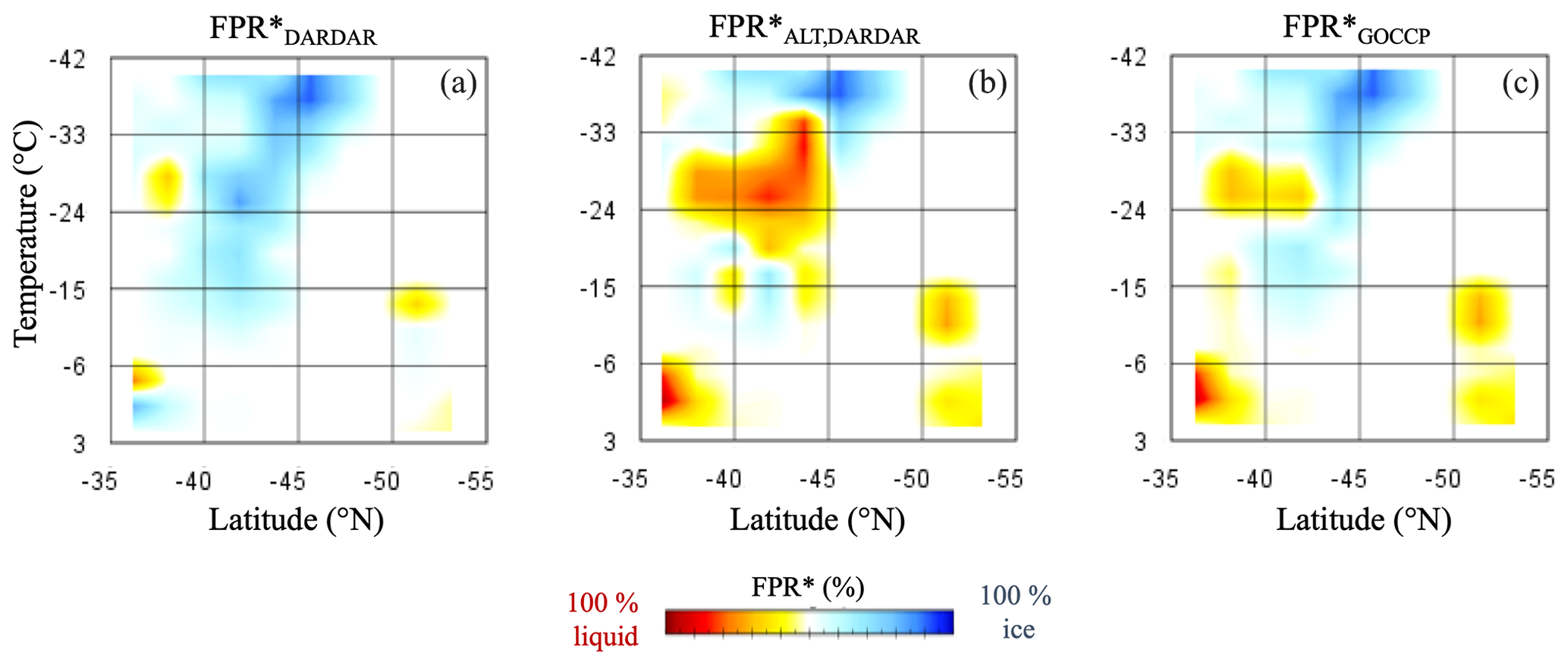

A4 Case study comparison
Some major differences can be observed between the three FPR* variables in Fig. A1d–f. For the altocumulus cloud at 35–40∘ S and +3 to −6 ∘C, the ice virgae falling from the cloud (FPRDARDAR) are missed in the FPRGOCCP. Such mixed-phase clouds are reclassified in FPRALT,DARDAR as liquid clouds. A similar case is observed for the stratocumulus clouds at 50–55∘ S and +3 to −6 ∘C and for the altostratus at 35–45∘ S below the −20 ∘C isotherm (at higher temperatures). Finally, the cirrus clouds above −33 ∘C remain nearly unaffected by the reclassification in FPRALT,DARDAR as it is classified as fully glaciated. Clouds between 38 and 44∘ S, ranging from 6 to −33 ∘C in temperature, are classified mostly as altostratus by the 2B-CLDCLASS product. These altostratus clouds offer a good opportunity to compare the three FPR variables in detail.
A4.1 FPRGOCCP
The detected ice virgae below the liquid cloud top suggest that the cloud top did not fully attenuate the lidar signal (not optically thick enough). The number or size of the ice particles near the cloud top probably was not enough to increase the depolarization ratio above the threshold value for the GOCCP algorithm, and it was therefore classified as liquid.
A4.2 FPRDARDAR
In the decision tree of the DARDAR algorithm, there are multiple alternatives for a mixture of cloud droplets and ice particles (e.g. at cloud top) to be classified as ice only.
- a.
If the lidar backscatter signal is lower than 2×10⁵ m−1 sr−1.
- b.
If not (a), it is weakly attenuated (less than 10 times) or not rapidly attenuated (at a depth larger than 480 m).
- c.
If not (b), the layer thickness of the cloud is larger than 300 m. This is equivalent to five voxels with a lidar vertical resolution of 60 m.
Therefore, there are many cases where a mixed-phase cloud can be misclassified as ice only in the DARDAR product and consequently in the FPRDARDAR variable. This misclassification may happen, for example, in optically thin stratiform cloud containing liquid. In this specific case, we speculate that point (c) is the most probable cause because of the large vertical extent of the clouds around 1 to 5 km using a moist adiabatic lapse rate of −6 K km−1 for the estimation.
A4.3 FPRALT,DARDAR
In the case of droplets and ice particles coexisting at cloud top, we expect that at some location the cloud droplets will be enough in number for one of the voxels to be classified as liquid (strong attenuation) in the DARDAR-MASK algorithm. If this is the case, the entire volume grid box value of FPRALT,DARDAR will be liquid. We interpret this as cloud that is not completely glaciated.
Table A1Summary of the different variables used to assess the frequency phase ratio (FPR).
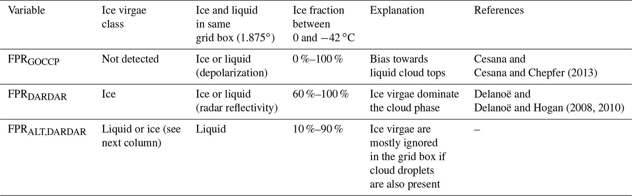

In summary, the GOCCP algorithm is unable to detect ice in mixed-phase clouds, and the DARDAR algorithm tends to classify mixed-phase clouds as ice. Therefore, we avoid using the frequency of cloud ice (FPR) to compare the GOCCP and DARDAR products. Instead, we use the FPRALT,DARDAR as common ground. In FPRALT,DARDAR, a significant portion of mixed-phase clouds that would otherwise be classified as ice is now classified as liquid. This replicates the inability of the GOCCP algorithm to detect ice in mixed-phase clouds. In other words, the frequency of completely glaciated clouds, which is represented by FPRALT,DARDAR and FPRGOCCP, allows for a comparison of both algorithms, mostly by ignoring ice virgae in FPRALT,DARDAR when cloud droplets are also present in the same grid box. This idea is summarized in Table A1. It is important to note that the behaviour of FPRALT,DARDAR is highly sensitive to the grid box volume, i.e. to the horizontal and vertical resolution. Calculated in finer resolutions, the FPRALT,DARDAR will be closer to FPRDARDAR. With coarser resolutions, the FPRALT,DARDAR will be biased towards the liquid phase because the probability of including an ice voxel in the volume grid boxes will increase. A grid box volume of K is coarse enough to study stratiform clouds from mid-latitude frontal systems.
A5 Temperature comparison
For temperatures between −40 and 1.5 ∘C, the FPRDARDAR only decreases down to 60 % at 1.5 ∘C (see Fig. A2). This difference is partly due to the higher sensitivity of the radar to ice particles, especially falling ice. Additionally, in the DARDAR algorithm, water can be still classified as ice at +1.5 ∘C due to the melting layer being set to a wet-bulb temperature of 0 ∘C. This threshold allows for the detection of ice at temperatures slightly above 0 ∘C dry-bulb temperatures (named simply temperature in this work). For instance, at a relative humidity of 50 %, a temperature of about +2.5 ∘C would correspond to a wet-bulb temperature of −2.5 ∘C. Nevertheless, this last effect is not relevant for temperatures below freezing.
In contrast, FPRALT,DARDAR follows very closely the pattern of the FPRGOCCP down to −1.5 ∘C. The absolute differences of the global averaged FPRALT,DARDAR and FPRGOCCP are less than 10 % between −42 and 0 ∘C. This shows that the temperature dependence of the alternative phase ratio FPRALT,DARDAR and FPRGOCCP agree better than for FPRDARDAR. On average, within a volume grid box of K the presence of single liquid voxels in the DARDAR product often coincides with the classification of the entire volume grid box as liquid in the GOCCP product.
A6 Latitude comparison
As shown in Fig. A3b, at −15 ∘C, the local maxima for FPRALT,DARDAR are similar to FPRGOCCP but occur at higher latitudes, at 61∘ S and 61∘ N with values of 69 % and 74 %. In comparison, the differences between FPRGOCCP and FPRALT,DARDAR at −15 ∘C are much lower than at −30 ∘C. Moreover, the FPRGOCCP at −15 ∘C is lower than the FPRALT,DARDAR at the southern mid-latitudes and northern high latitudes. In conclusion, the DARDAR and CALIPSO-GOCCP products still differ in some important aspects. However, to simplify the reproducibility of our study, we only present the results for CALIPSO-GOCCP, which is already available at a horizontal grid and 3 K vertical levels.
All datasets used in the analysis are freely available at (last access: 13 February 2019):
-
http://climserv.ipsl.polytechnique.fr/cfmip-obs/Calipso_goccp_new.html (Chepfer, 2019)
-
http://www.icare.univ-lille1.fr/archive (Université de Lille, 2019)
-
http://apps.ecmwf.int/datasets/data/macc-reanalysis/levtype=ml (CAMS, 2019)
-
https://apps.ecmwf.int/datasets/data/interim-full-daily/levtype=pl/ (ECMWF, 2019)
The supplement related to this article is available online at: https://doi.org/10.5194/acp-20-2177-2020-supplement.
IT, BH, PS, and DV contributed to the design of the study. DV processed the datasets, performed the analysis, designed the figures, and drafted the paper. All authors contributed valuable feedback throughout the process. All authors helped with the discussion of the results and contributed to the final paper.
The authors declare that they have no conflict of interest.
We thank the GOCCP project for providing access to the CALIPSO-GOCCP gridded cloud-phase profiles. We thank the NASA CloudSat project and the CloudSat Data Processing Center for providing access to the 2B-CLDCLASS product. We thank the ICARE Data and Services Center for providing access to the DARDAR and CloudSat data. We thank the MACC project and the ERA-Interim science team for providing access to the reanalysis data. We thank Albert Ansmann, Johannes Mülmenstädt, and Julien Delanoë for helpful discussions. The authors would like to thank the editor and anonymous referee no. 4 from the first version of the paper for suggesting the inclusion of constraints for humidity and static stability, which greatly improved the accuracy of the results.
The publication of this article was funded by the
Open Access Fund of the Leibniz Association.
This paper was edited by Matthias Tesche and reviewed by two anonymous referees.
Albani, S., Mahowald, N. M., Delmonte, B., Maggi, V., and Winckler, G.: Comparing modeled and observed changes in mineral dust transport and deposition to Antarctica between the Last Glacial Maximum and current climates, Clim. Dynam., 38, 1731–1755, https://doi.org/10.1007/s00382-011-1139-5, 2012. a
Ansmann, A., Tesche, M., Althausen, D., Müller, D., Seifert, P., Freudenthaler, V., Heese, B., Wiegner, M., Pisani, G., Knippertz, P., and Dubovik, O.: Influence of Saharan dust on cloud glaciation in southern Morocco during the Saharan Mineral Dust Experiment, J. Geophys. Res.-Atmos., 113, https://doi.org/10.1029/2007JD008785, 2008. a, b
Ansmann, A., Rittmeister, F., Engelmann, R., Basart, S., Jorba, O., Spyrou, C., Remy, S., Skupin, A., Baars, H., Seifert, P., Senf, F., and Kanitz, T.: Profiling of Saharan dust from the Caribbean to western Africa – Part 2: Shipborne lidar measurements versus forecasts, Atmos. Chem. Phys., 17, 14987–15006, https://doi.org/10.5194/acp-17-14987-2017, 2017. a, b
Atkinson, J. D., Murray, B. J., Woodhouse, M. T., Whale, T. F., Baustian, K. J., Carslaw, K. S., Dobbie, S., O'Sullivan, D., and Malkin, T. L.: The importance of feldspar for ice nucleation by mineral dust in mixed-phase clouds, Nature, 498, 355–358, https://doi.org/10.1038/nature12278, 2013. a, b, c
Augustin-Bauditz, S., Wex, H., Denjean, C., Hartmann, S., Schneider, J., Schmidt, S., Ebert, M., and Stratmann, F.: Laboratory-generated mixtures of mineral dust particles with biological substances: characterization of the particle mixing state and immersion freezing behavior, Atmos. Chem. Phys., 16, 5531–5543, https://doi.org/10.5194/acp-16-5531-2016, 2016. a
Barahona, D., Molod, A., and Kalesse, H.: Direct estimation of the global distribution of vertical velocity within cirrus clouds, Sci. Rep., 7, https://doi.org/10.1038/s41598-017-07038-6, 2017. a
Boose, Y., Welti, A., Atkinson, J., Ramelli, F., Danielczok, A., Bingemer, H. G., Plötze, M., Sierau, B., Kanji, Z. A., and Lohmann, U.: Heterogeneous ice nucleation on dust particles sourced from nine deserts worldwide – Part 1: Immersion freezing, Atmos. Chem. Phys., 16, 15075–15095, https://doi.org/10.5194/acp-16-15075-2016, 2016. a, b, c
Bosilovich, M. G., Robertson, F. R., and Chen, J.: Global energy and water budgets in MERRA, J. Climate, 24, https://doi.org/10.1175/2011JCLI4175.1, 2011. a
Broadley, S. L., Murray, B. J., Herbert, R. J., Atkinson, J. D., Dobbie, S., Malkin, T. L., Condliffe, E., and Neve, L.: Immersion mode heterogeneous ice nucleation by an illite rich powder representative of atmospheric mineral dust, Atmos. Chem. Phys., 12, 287–307, https://doi.org/10.5194/acp-12-287-2012, 2012. a
Bühl, J., Seifert, P., Myagkov, A., and Ansmann, A.: Measuring ice- and liquid-water properties in mixed-phase cloud layers at the Leipzig Cloudnet station, Atmos. Chem. Phys., 16, 10609–10620, https://doi.org/10.5194/acp-16-10609-2016, 2016. a
Burrows, S. M., Hoose, C., Pöschl, U., and Lawrence, M. G.: Ice nuclei in marine air: biogenic particles or dust?, Atmos. Chem. Phys., 13, 245–267, https://doi.org/10.5194/acp-13-245-2013, 2013. a, b
Cesana, G. and Chepfer, H.: Evaluation of the cloud thermodynamic phase in a climate model using CALIPSO-GOCCP, J. Geophys. Res.-Atmos., 118, 7922–7937, https://doi.org/10.1002/jgrd.50376, 2013. a, b, c
Cesana, G., Waliser, D. E., Jiang, X., and Li, J. L.: Multimodel evaluation of cloud phase transition using satellite and reanalysis data, J. Geophys. Res., 120, 7871–7892, https://doi.org/10.1002/2014JD022932, 2015. a, b
Chepfer, H.: GCM-Oriented CALIPSO Cloud Product, available at: https://climserv.ipsl.polytechnique.fr/cfmip-obs/Calipso_goccp_new.html, last access: 13 February 2019.
Choi, Y.-S., Lindzen, R. S., Ho, C.-H., and Kim, J.: Space observations of cold-cloud phase change, P. Natl. Acad. Sci. USA, 107, 11211–11216, https://doi.org/10.1073/pnas.1006241107, 2010. a, b, c, d, e
Claquin, T., Schulz, M., and Balkanski, Y. J.: Modeling the mineralogy of atmospheric dust sources, J. Geophys. Res.-Atmos., 104, https://doi.org/10.1029/1999JD900416, 1999. a, b
Copernicus Atmosphere Monitoring Service (CAMS): MACC-II Consortium, 2011: MACC Reanalysis of Global Atmospheric Composition (2003–2012), available at: http://apps.ecmwf.int/datasets/data/macc-reanalysis/levtype=ml, last access: 13 February 2019.
Cuevas, E., Camino, C., Benedetti, A., Basart, S., Terradellas, E., Baldasano, J. M., Morcrette, J. J., Marticorena, B., Goloub, P., Mortier, A., Berjón, A., Hernández, Y., Gil-Ojeda, M., and Schulz, M.: The MACC-II 2007–2008 reanalysis: atmospheric dust evaluation and characterization over northern Africa and the Middle East, Atmos. Chem. Phys., 15, 3991–4024, https://doi.org/10.5194/acp-15-3991-2015, 2015. a, b
De Boer, G., Morrison, H., Shupe, M. D., and Hildner, R.: Evidence of liquid dependent ice nucleation in high-latitude stratiform clouds from surface remote sensors, Geophys. Res. Lett., 38, https://doi.org/10.1029/2010GL046016, 2011. a, b
Dee, D. P., Uppala, S. M., Simmons, A. J., Berrisford, P., Poli, P., Kobayashi, S., Andrae, U., Balmaseda, M. A., Balsamo, G., Bauer, P., Bechtold, P., Beljaars, A. C. M., van de Berg, L., Bidlot, J., Bormann, N., Delsol, C., Dragani, R., Fuentes, M., Geer, A. J., Haimberger, L., Healy, S. B., Hersbach, H., Hólm, E. V., Isaksen, L., Kållberg, P., Köhler, M., Matricardi, M., McNally, A. P., Monge-Sanz, B. M., Morcrette, J.-J., Park, B.-K., Peubey, C., de Rosnay, P., Tavolato, C., Thépaut, J.-N., and Vitart, F.: The ERA-Interim reanalysis: configuration and performance of the data assimilation system, Q. J. Roy. Meteor. Soc., 137, 553–597, https://doi.org/10.1002/qj.828, 2011. a
Delanoë, J. and Hogan, R. J.: Combined CloudSat-CALIPSO-MODIS retrievals of the properties of ice clouds, J. Geophys. Res.-Atmos., 115, https://doi.org/10.1029/2009JD012346, 2010.
Delanoë, J. M. E. and Hogan, R. J.: A variational scheme for retrieving ice cloud properties from combined radar, lidar, and infrared radiometer, J. Geophys. Res.-Atmos., 113, https://doi.org/10.1029/2007JD009000, 2008.
Diehl, K. and Wurzler, S.: Heterogeneous Drop Freezing in the Immersion Mode: Model Calculations Considering Soluble and Insoluble Particles in the Drops, J. Atmos. Sci., 61, https://doi.org/10.1175/1520-0469(2004)061<2063:hdfiti>2.0.co;2, 2004. a
Diehl, K., Simmel, M., and Wurzler, S.: Numerical sensitivity studies on the impact of aerosol properties and drop freezing modes on the glaciation, microphysics and dynamics of clouds, J. Geophys. Res.-Atmos., 111, https://doi.org/10.1029/2005JD005884, 2006. a
Dietlicher, R., Neubauer, D., and Lohmann, U.: Elucidating ice formation pathways in the aerosol–climate model ECHAM6-HAM2, Atmos. Chem. Phys., 19, 9061–9080, https://doi.org/10.5194/acp-19-9061-2019, 2019. a
Dubovik, O., Smirnov, A., Holben, B. N., King, M. D., Kaufman, Y. J., Eck, T. F., and Slutsker, I.: Accuracy assessments of aerosol optical properties retrieved from Aerosol Robotic Network (AERONET) Sun and sky radiance measurements, J. Geophys. Res.-Atmos., 105, 9791–9806, https://doi.org/10.1029/2000JD900040, 2000. a
ECMWF: ERA-Interim, available at: https://apps.ecmwf.int/datasets/data/interim-full-daily/levtype=pl/, last access: 13 February 2019.
Eskes, H., Huijnen, V., Arola, A., Benedictow, A., Blechschmidt, A.-M., Botek, E., Boucher, O., Bouarar, I., Chabrillat, S., Cuevas, E., Engelen, R., Flentje, H., Gaudel, A., Griesfeller, J., Jones, L., Kapsomenakis, J., Katragkou, E., Kinne, S., Langerock, B., Razinger, M., Richter, A., Schultz, M., Schulz, M., Sudarchikova, N., Thouret, V., Vrekoussis, M., Wagner, A., and Zerefos, C.: Validation of reactive gases and aerosols in the MACC global analysis and forecast system, Geosci. Model Dev., 8, 3523–3543, https://doi.org/10.5194/gmd-8-3523-2015, 2015. a
Fröhlich-Nowoisky, J., Hill, T. C. J., Pummer, B. G., Yordanova, P., Franc, G. D., and Pöschl, U.: Ice nucleation activity in the widespread soil fungus Mortierella alpina, Biogeosciences, 12, 1057–1071, https://doi.org/10.5194/bg-12-1057-2015, 2015. a
Georgoulias, A. K., Tsikerdekis, A., Amiridis, V., Marinou, E., Benedetti, A., Zanis, P., Alexandri, G., Mona, L., Kourtidis, K. A., and Lelieveld, J.: A 3-D evaluation of the MACC reanalysis dust product over Europe, northern Africa and Middle East using CALIOP/CALIPSO dust satellite observations, Atmos. Chem. Phys., 18, 8601–8620, https://doi.org/10.5194/acp-18-8601-2018, 2018. a
Gryspeerdt, E., Quaas, J., and Bellouin, N.: Constraining the aerosol influence on cloud fraction, J. Geophys. Res., 121, https://doi.org/10.1002/2015JD023744, 2016. a, b
Hartmann, S., Wex, H., Clauss, T., Augustin-Bauditz, S., Niedermeier, D., Rösch, M., and Stratmann, F.: Immersion Freezing of Kaolinite: Scaling with Particle Surface Area, J. Atmos. Sci., 73, https://doi.org/10.1175/JAS-D-15-0057.1, 2016. a
Hauke, J. and Kossowski, T.: Comparison of values of pearson's and spearman's correlation coefficients on the same sets of data, Quaestiones Geographicae, 30, https://doi.org/10.2478/v10117-011-0021-1, 2011. a
Hoose, C. and Möhler, O.: Heterogeneous ice nucleation on atmospheric aerosols: a review of results from laboratory experiments, Atmos. Chem. Phys., 12, 9817–9854, https://doi.org/10.5194/acp-12-9817-2012, 2012. a, b
Hoose, C., Lohmann, U., Erdin, R., and Tegen, I.: The global influence of dust mineralogical composition on heterogeneous ice nucleation in mixed-phase clouds, Environ. Res. Lett., 3, https://doi.org/10.1088/1748-9326/3/2/025003, 2008. a, b
Hu, Y., Rodier, S., Xu, K. M., Sun, W., Huang, J., Lin, B., Zhai, P., and Josset, D.: Occurrence, liquid water content, and fraction of supercooled water clouds from combined CALIOP/IIR/MODIS measurements, J. Geophys. Res.-Atmos., 115, https://doi.org/10.1029/2009JD012384, 2010. a
Huang, L., Jiang, J. H., Wang, Z., Su, H., Deng, M., and Massie, S.: Climatology of cloud water content associated with different cloud types observed by A-Train satellites, J. Geophys. Res., 120, https://doi.org/10.1002/2014JD022779, 2015. a, b
Huang, Y., Siems, S. T., Manton, M. J., Protat, A., and Delanoë, J.: A study on the low-altitude clouds over the Southern Ocean using the DARDAR-MASK, J. Geophys. Res.-Atmos., 117, 117, https://doi.org/10.1029/2012JD017800, 2012. a
Johnson, M. S., Meskhidze, N., Kiliyanpilakkil, V. P., and Gassó, S.: Understanding the transport of Patagonian dust and its influence on marine biological activity in the South Atlantic Ocean, Atmos. Chem. Phys., 11, 2487–2502, https://doi.org/10.5194/acp-11-2487-2011, 2011. a
Kanitz, T., Seifert, P., Ansmann, A., Engelmann, R., Althausen, D., Casiccia, C., and Rohwer, E. G.: Contrasting the impact of aerosols at northern and southern midlatitudes on heterogeneous ice formation, Geophys. Res. Lett., 38, https://doi.org/10.1029/2011GL048532, 2011. a, b, c, d
Klein, S. A. and Hartmann, D. L.: The seasonal cycle of low stratiform clouds, J. Climate, 6, https://doi.org/10.1175/1520-0442(1993)006<1587:TSCOLS>2.0.CO;2, 1993. a, b
Kok, J. F.: A scaling theory for the size distribution of emitted dust aerosols suggests climate models underestimate the size of the global dust cycle, P. Natl. Acad. Sci. USA, 108, 1016–1021, https://doi.org/10.1073/pnas.1014798108, 2011. a
Korolev, A., McFarquhar, G., Field, P. R., Franklin, C., Lawson, P., Wang, Z., Williams, E., Abel, S. J., Axisa, D., Borrmann, S., Crosier, J., Fugal, J., Krämer, M., Lohmann, U., Schlenczek, O., Schnaiter, M., Wendisch, M., Korolev, A., McFarquhar, G., Field, P. R., Franklin, C., Lawson, P., Wang, Z., Williams, E., Abel, S. J., Axisa, D., Borrmann, S., Crosier, J., Fugal, J., Krämer, M., Lohmann, U., Schlenczek, O., Schnaiter, M., and Wendisch, M.: Mixed-Phase Clouds: Progress and Challenges, Meteorological Monographs, 58, 5.1–5.50, https://doi.org/10.1175/AMSMONOGRAPHS-D-17-0001.1, 2017. a, b
Lacher, L., DeMott, P. J., Levin, E. J. T., Suski, K. J., Boose, Y., Zipori, A., Herrmann, E., Bukowiecki, N., Steinbacher, M., Gute, E., Abbatt, J. P. D., Lohmann, U., and Kanji, Z. A.: Background Free Tropospheric Ice Nucleating Particle Concentrations at Mixed phase Cloud Conditions, J. Geophys. Res.-Atmos., 123, https://doi.org/10.1029/2018JD028338, 2018. a
Li, F., Ginoux, P., and Ramaswamy, V.: Distribution, transport, and deposition of mineral dust in the Southern Ocean and Antarctica: Contribution of major sources, J. Geophys. Res.-Atmos., 113, https://doi.org/10.1029/2007JD009190, 2008. a
Li, J., Lv, Q., Zhang, M., Wang, T., Kawamoto, K., Chen, S., and Zhang, B.: Effects of atmospheric dynamics and aerosols on the fraction of supercooled water clouds, Atmos. Chem. Phys., 17, 1847–1863, https://doi.org/10.5194/acp-17-1847-2017, 2017a. a, b, c, d, e
Li, R., Dong, X., Guo, J., Fu, Y., Zhao, C., Wang, Y., and Min, Q.: The implications of dust ice nuclei effect on cloud top temperature in a complex mesoscale convective system, Sci. Rep., 7, https://doi.org/10.1038/s41598-017-12681-0, 2017b. a
Mahowald, N., Albani, S., Kok, J. F., Engelstaeder, S., Scanza, R., Ward, D. S., and Flanner, M. G.: The size distribution of desert dust aerosols and its impact on the Earth system, Aeolian Res., 15, 53–71, https://doi.org/10.1016/j.aeolia.2013.09.002, 2014. a, b
McCoy, D. T., Tan, I., Hartmann, D. L., Zelinka, M. D., and Storelvmo, T.: On the relationships among cloud cover, mixed-phase partitioning, and planetary albedo in GCMs, J. Adv. Model. Earth Sy., 8, https://doi.org/10.1002/2015MS000589, 2016. a
Morrison, A. E., Siems, S. T., and Manton, M. J.: A three-year climatology of cloud-top phase over the Southern Ocean and North Pacific, J. Climate, 24, 2405–2418, https://doi.org/10.1175/2010JCLI3842.1, 2011. a
Murray, B. J., Broadley, S. L., Wilson, T. W., Atkinson, J. D., and Wills, R. H.: Heterogeneous freezing of water droplets containing kaolinite particles, Atmos. Chem. Phys., 11, 4191–4207, https://doi.org/10.5194/acp-11-4191-2011, 2011. a, b
Niedermeier, D., Shaw, R. A., Hartmann, S., Wex, H., Clauss, T., Voigtländer, J., and Stratmann, F.: Heterogeneous ice nucleation: exploring the transition from stochastic to singular freezing behavior, Atmos. Chem. Phys., 11, 8767–8775, https://doi.org/10.5194/acp-11-8767-2011, 2011. a
Niedermeier, D., Augustin-Bauditz, S., Hartmann, S., Wex, H., Ignatius, K., and Stratmann, F.: Can we define an asymptotic value for the ice active surface site density for heterogeneous ice nucleation?, J. Geophys. Res., 210, https://doi.org/10.1002/2014JD022814, 2015. a
Niemand, M., Möhler, O., Vogel, B., Vogel, H., Hoose, C., Connolly, P., Klein, H., Bingemer, H., DeMott, P., Skrotzki, J., and Leisner, T.: A Particle-Surface-Area-Based Parameterization of Immersion Freezing on Desert Dust Particles, J. Atmos. Sci., 69, https://doi.org/10.1175/JAS-D-11-0249.1, 2012. a
O'Sullivan, D., Adams, M. P., Tarn, M. D., Harrison, A. D., Vergara-Temprado, J., Porter, G. C. E., Holden, M. A., Sanchez-Marroquin, A., Carotenuto, F., Whale, T. F., McQuaid, J. B., Walshaw, R., Hedges, D. H. P., Burke, I. T., Cui, Z., and Murray, B. J.: Contributions of biogenic material to the atmospheric ice-nucleating particle population in North Western Europe, Sci. Rep., 8, 13821, https://doi.org/10.1038/s41598-018-31981-7, 2018. a
Petters, M. D. and Wright, T. P.: Revisiting ice nucleation from precipitation samples, Geophys. Res. Lett., 42, https://doi.org/10.1002/2015GL065733, 2015. a
Price, H. C., Baustian, K. J., McQuaid, J. B., Blyth, A., Bower, K. N., Choularton, T., Cotton, R. J., Cui, Z., Field, P. R., Gallagher, M., Hawker, R., Merrington, A., Miltenberger, A., Neely, R. R., Parker, S. T., Rosenberg, P. D., Taylor, J. W., Trembath, J., Vergara-Temprado, J., Whale, T. F., Wilson, T. W., Young, G., and Murray, B. J.: Atmospheric Ice-Nucleating Particles in the Dusty Tropical Atlantic, J. Geophys. Res.- Atmos., 123, https://doi.org/10.1002/2017JD027560, 2018. a
Randall, D. A., Wood, R. A., Bony, S., Colman, R., Fichefet, T., Fyve, J., Kattsov, V., Pitman, A., Shukla, J., Srinivasan, J., Stouffer, R. J., Sumi, A., and Taylor, K. E.: Climate Models and Their Evaluation, Climate Change 2007: The Physical Science Basis. Contribution of Working Group I to the Fourth Assessment Report of the Intergovernmental Panel on Climate Change, https://doi.org/10.1016/j.cub.2007.06.045, 2007. a
Ridley, D. A., Heald, C. L., Kok, J. F., and Zhao, C.: An observationally constrained estimate of global dust aerosol optical depth, Atmos. Chem. Phys., 16, 15097–15117, https://doi.org/10.5194/acp-16-15097-2016, 2016. a
Sassen, K. and Wang, Z.: Classifying clouds around the globe with the CloudSat radar: 1-year of results, Geophys. Res. Lett., 35, https://doi.org/10.1029/2007GL032591, 2008. a
Scott, R. C. and Lubin, D.: Unique manifestations of mixed-phase cloud microphysics over Ross Island and the Ross Ice Shelf, Antarctica, Geophys. Res. Lett., 43, https://doi.org/10.1002/2015GL067246, 2016. a
Seifert, P., Ansmann, A., Mattis, I., Wandinger, U., Tesche, M., Engelmann, R., Müller, D., Pérez, C., and Haustein, K.: Saharan dust and heterogeneous ice formation: Eleven years of cloud observations at a central European EARLINET site, J. Geophys. Res.-Atmos., 115, https://doi.org/10.1029/2009JD013222, 2010. a, b, c, d
Seinfeld, J. H. and Pandis, S. N.: Atmospheric Chemistry and Physics: From Air Pollution to Climate Change, Atmospheric chemistry and physics from air pollution to climate change, New York, NY, Wiley 1998, Physical description, xxvii, 1326 p., A WileyInterscience Publication, ISBN 0471178152, 51, 1–4, https://doi.org/10.1080/00139157.1999.10544295, 1998. a
Sullivan, S. C., Lee, D., Oreopoulos, L., and Nenes, A.: Role of updraft velocity in temporal variability of global cloud hydrometeor number, P. Natl. Acad. Sci. USA, 113, 5791–5796, https://doi.org/10.1073/pnas.1514039113, 2016. a
Tan, I., Storelvmo, T., and Choi, Y. S.: Spaceborne lidar observations of the ice-nucleating potential of dust, polluted dust, and smoke aerosols in mixed-phase clouds, J. Geophys. Res., 119, 6653–6665, https://doi.org/10.1002/2013JD021333, 2014. a, b, c, d, e, f, g, h
Toth, T. D., Campbell, J. R., Reid, J. S., Tackett, J. L., Vaughan, M. A., Zhang, J., and Marquis, J. W.: Minimum aerosol layer detection sensitivities and their subsequent impacts on aerosol optical thickness retrievals in CALIPSO level 2 data products, Atmos. Meas. Tech., 11, 499–514, https://doi.org/10.5194/amt-11-499-2018, 2018. a
Université de Lille: ICARE Data and Services Center, available at: http://www.icare.univ-lille1.fr/contacts, last access: 13 February 2019.
Vergara-Temprado, J., Murray, B. J., Wilson, T. W., O'Sullivan, D., Browse, J., Pringle, K. J., Ardon-Dryer, K., Bertram, A. K., Burrows, S. M., Ceburnis, D., DeMott, P. J., Mason, R. H., O'Dowd, C. D., Rinaldi, M., and Carslaw, K. S.: Contribution of feldspar and marine organic aerosols to global ice nucleating particle concentrations, Atmos. Chem. Phys., 17, 3637–3658, https://doi.org/10.5194/acp-17-3637-2017, 2017. a, b, c, d
Vergara-Temprado, J., Miltenberger, A. K., Furtado, K., Grosvenor, D. P., Shipway, B. J., Hill, A. A., Wilkinson, J. M., Field, P. R., Murray, B. J., and Carslaw, K. S.: Strong control of Southern Ocean cloud reflectivity by ice-nucleating particles, P. Natl. Acad. Sci. USA, 115, 201721627, https://doi.org/10.1073/pnas.1721627115, 2018. a
Welti, A., Lüönd, F., Stetzer, O., and Lohmann, U.: Influence of particle size on the ice nucleating ability of mineral dusts, Atmos. Chem. Phys., 9, 6705–6715, https://doi.org/10.5194/acp-9-6705-2009, 2009. a
Westbrook, C. D. and Illingworth, A. J.: Evidence that ice forms primarily in supercooled liquid clouds at temperatures > 27∘C, Geophys. Res. Lett., 38, https://doi.org/10.1029/2011GL048021, 2011. a, b, c
Wu, Y., Cordero, L., Gross, B., Moshary, F., and Ahmed, S.: Assessment of CALIPSO attenuated backscatter and aerosol retrievals with a combined ground-based multi-wavelength lidar and sunphotometer measurement, Atmos. Environ., 84, 44–53, https://doi.org/10.1016/j.atmosenv.2013.11.016, 2014. a
Zamora, L. M., Kahn, R. A., Huebert, K. B., Stohl, A., and Eckhardt, S.: A satellite-based estimate of combustion aerosol cloud microphysical effects over the Arctic Ocean, Atmos. Chem. Phys., 18, 14949–14964, https://doi.org/10.5194/acp-18-14949-2018, 2018. a
Zhang, D., Wang, Z., and Liu, D.: A global view of midlevel liquid-layer topped stratiform cloud distribution and phase partition from CALIPSO and CloudSat measurements, J. Geophys. Res.-Atmos., 115, https://doi.org/10.1029/2009JD012143, 2010. a, b
Zhang, D., Wang, Z., Heymsfield, A., Fan, J., Liu, D., and Zhao, M.: Quantifying the impact of dust on heterogeneous ice generation in midlevel supercooled stratiform clouds, Geophys. Res. Lett., 39, https://doi.org/10.1029/2012GL052831, 2012. a, b, c
Zhang, D., Liu, D., Luo, T., Wang, Z., and Yin, Y.: Aerosol impacts on cloud thermodynamic phase change over East Asia observed with CALIPSO and CloudSat measurements, J. Geophys. Res., 120, 1490–1501, https://doi.org/10.1002/2014JD022630, 2015. a
Zhang, D., Wang, Z., Kollias, P., Vogelmann, A. M., Yang, K., and Luo, T.: Ice particle production in mid-level stratiform mixed-phase clouds observed with collocated A-Train measurements, Atmos. Chem. Phys., 18, 4317–4327, https://doi.org/10.5194/acp-18-4317-2018, 2018. a, b, c