Simulation of convective moistening of the extratropical lower stratosphere using a numerical weather prediction model

Stratospheric water vapour (SWV) is a climatically important atmospheric constituent due to its impacts on the radiation budget and atmospheric chemical composition. Despite the important role of SWV in the climate system, the processes controlling the distribution and variation in water vapour in the upper troposphere and lower stratosphere (UTLS) are not well understood. In order to better understand the mechanism of transport of water vapour through the tropopause, this study uses the high-resolution Global Environmental Multiscale model of the Environment and Climate Change Canada to simulate a lower stratosphere moistening event over North America. Satellite remote sensing and aircraft in situ observations are used to evaluate the quality of model simulation. The main focus of this study is to evaluate the processes that influence the lower stratosphere water vapour budget, particularly the direct water vapour transport and the moistening due to the ice sublimation. In the high-resolution simulations with horizontal grid spacing of less than 2.5 km, it is found that the main contribution to lower stratospheric moistening is the upward transport caused by the breaking of gravity waves. In contrast, for the lower-resolution simulation with horizontal grid spacing of 10 km, the lower stratospheric moistening is dominated by the sublimation of ice. In comparison with the aircraft in situ observations, the high-resolution simulations predict the water vapour content in the UTLS well, while the lower-resolution simulation overestimates the water vapour content. This overestimation is associated with the overly abundant ice in the UTLS along with a sublimation rate that is too high in the lower stratosphere. The results of this study affirm the strong influence of overshooting convection on the lower stratospheric water vapour and highlight the importance of both dynamics and microphysics in simulating the water vapour distribution in the UTLS region.

1 Introduction

Stratospheric water vapour (SWV) strongly influences the Earth radiation budget (IPCC, 2013) and stratospheric chemistry (e.g., Anderson et al., 2012). Global climate models (GCMs) generally project an increase in SWV during global warming, which may lead to cooling of the stratosphere and further warming of the troposphere and surface (Forster and Shine, 1999, 2002; Solomon et al., 2010; Riese et al., 2012) and thus constitutes a potentially important climate feedback mechanism (Dessler et al., 2013; Huang 2013; Huang et al., 2016; Banerjee et al., 2019). Dessler et al. (2013) estimated the SWV feedback to be +0.3 W m⁻² K⁻¹. Especially emphasized in these previous studies is the importance of SWV in the extratropical lowermost stratosphere, which has the most significant impact on the energy budget at the top of the atmosphere.

Despite its importance, the processes that control the distribution and variation in water vapour in the upper troposphere and lower stratosphere (UTLS) are not well understood. Large discrepancies are found between the “A-Train” satellite observations and the GCMs of Phase 5 of the Coupled Model Inter-comparison Project (CMIP5) (Jiang, 2012). This study shows that the ratio of water vapour content in the GCMs to that from satellite observations can be as large as two to five in the mid-latitude UTLS region. Such discrepancies cast significant uncertainty in the SWV radiative feedback simulated by the GCMs (Huang et al., 2016). Global reanalyses also suffer from SWV biases, including the Modern-Era Retrospective Analysis for Research and Applications (MERRA), its newer release MERRA2 and the Interim Reanalysis of the European Centre for Medium-Range Weather Forecasts (ECMWF) (Jiang et al., 2015). One of the motivations of this study is therefore to investigate the possible causes of such overestimation of water vapour in the UTLS in GCMs and numerical weather prediction (NWP) models.

The mechanisms controlling the transport of water vapour into the stratosphere are different for tropical and mid-latitude regions. In the tropical region, water vapour enters the stratosphere primarily through the slow ascent associated with the Brewer–Dobson circulation (BDC) (Brewer, 1949). The cold temperature of the tropical tropopause layer (TTL) regulates the humidity of the air and therefore is responsible for the moistening of the stratosphere. However, it remains uncertain how factors such as the temperature in the TTL, strength of the BDC, and the vertical and horizontal mixing are weighted to determine SWV distribution and variation (Fueglistaler et al., 2014). In the extratropical region, there are several mechanisms that can influence the distribution and variation in the water vapour in the lower stratosphere (Weinstock et al., 2007). Water can be transported to the lowermost extratropical stratosphere by poleward transport from the TTL, by isentropic transport due to planetary wave activity from the tropical troposphere and by deep convection in the extratropics. Among these mechanisms, the vertical transport by mid-latitude convection, although demonstrated to be impactful by studies using in situ and remote sensing measurements, remains poorly understood (Poulida et al., 1996; Hegglin et al., 2004; Dessler and Sherwood, 2004; Ray et al., 2004; Hanisco et al., 2007; Weinstock et al., 2007; Homeyer et al., 2014, 2017; Sun and Huang, 2015; Smith et al., 2017).

A few studies have attempted to simulate the injection of water into the lower stratosphere using high-resolution NWP models. These studies found that the transport of water vapour into the stratosphere occurs through gravity wave breaking near overshooting tops (e.g., Wang, 2003; Wang et al., 2009, 2011; Homeyer et al., 2017; Dauhut et al., 2018; Lee et al., 2019). The overshooting tops form as strong updrafts within convective cells penetrate the stable stratification at the tropopause. They act as obstacles to the lower stratospheric flow and generate gravity waves. In favourable conditions (Baines, 1995; Sachsperger et al., 2015), the gravity waves break near the overshooting cloud tops, dissipate wave energy through strong turbulence and cause sudden “jumps” of air flow up to more than 2 km height. This upward wind with strong turbulence transports a substantial amount of water vapour and ice into higher altitudes in the stratosphere. The mechanism of gravity wave breaking is well demonstrated, e.g., by Fig. 7 in Wang (2003). An associated phenomenon is the so-called “jumping cirrus” (Fujita 1982), which provides evidence that ice particles are brought into and potentially hydrate the lower stratosphere. The mechanism of cross-tropopause transport of humidity associated with gravity wave breaking is generally well simulated, using idealized forcing for a short duration over a limited domain (Wang, 2003; Wang et al., 2009, 2011; Homeyer et al., 2017; Dauhut et al., 2018). In order to evaluate model results against satellite and aircraft measurements it is necessary to develop an experimental framework in which high-resolution simulations can be performed over an extended period in which observations are available.

In this study, we use a high-resolution NWP model, Global Environmental Multiscale (GEM), to simulate an observed lower stratospheric moistening event over North America from 26 to 27 August 2013 (Smith et al., 2017). The first objective is to evaluate the model capability to successfully simulate the vertical transport of water vapour through mid-latitude tropopause and reproduce the observed increase in lower stratospheric humidity during and after the deep convection event. The second objective is to evaluate, using all available satellite and aircraft measurements, the simulated water vapour fields at different horizontal resolutions, ranging from low resolution with parameterized deep convection to high resolutions with explicitly simulated convection. The third objective is to compare processes, such as direct water vapour transport vs. ice sublimation, that influence the lower stratosphere water vapour budget. In the global NWP and GCM models, the deep convection is parameterized using a mass flux approach. The complex phenomena near the tropopause during the convection are parameterized in a simplified manner, e.g., overshooting convection, or not parameterized, e.g., the falling of overshooting cloud tops (not sedimentation), gravity wave breaking and formation of jumping cirrus. In light of the aforementioned lower stratospheric humidity bias in coarse-resolution models, we are especially interested to identify possible causes of such biases.

This paper is structured as follows. The next section provides a brief description of the GEM model and the configuration of the simulation experiment, as well as the observation data for comparison and a trajectory model used to link the simulated and observed samples. This is followed by the analysis of the GEM simulation results, with a focus on the lower stratospheric water vapour budget. We then conclude with a summary of the findings and perspectives for further studies.

2 Method

2.1 NWP model simulation

The NWP model used in this study is the GEM model of Environment and Climate Change Canada (ECCC, Côté et al., 1998; Girard et al., 2014). The dynamics of GEM are formulated in terms of the non-hydrostatic primitive equations with a terrain-following hybrid vertical grid. It can be run as a global model or a limited-area model and is capable of one-way self-nesting. Milbrandt et al. (2016) described the self-nesting configuration with horizontal grid spacing Δx≥2.5 km; Leroyer et al. (2014) and Bélair et al. (2017) did the same for Δx=0.25 km. For the experiments reported here, four self-nested domains are used with areas of 5000 km× 3600 km, 3000 km × 2000 km, 1500 km × 1000 km and 375 km × 375 km, which corresponds to horizontal grid spacing of 10, 2.5, 1 and 0.25 km, respectively. The four nested domains are shown in Fig. 1. All simulations use 77 vertical levels, with vertical grid spacing Δz≈250 m in the UTLS region.

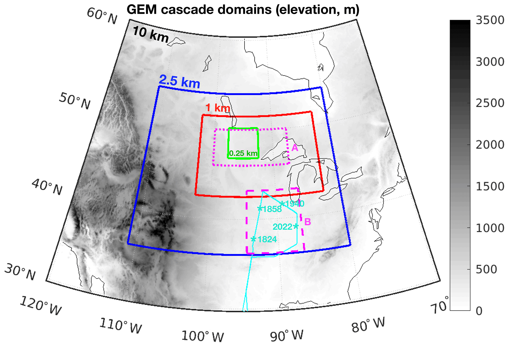
Figure 1 GEM cascade domains. Thick solid lines in black, blue, red and green represent simulation domains at 10, 2.5, 1 and 0.25 km horizontal grid spacing, respectively. The thin cyan line represents the ER-2 aircraft flight path on 27 August 2013. The dotted magenta line represents evaluation Domain A, which covers the major convective events of this study. The dashed magenta line represents Domain B for comparison between aircraft observations and model simulations. The four cyan stars show the locations and times (UTC) of the lowest location of the descending–ascending trajectories of the aircraft.

For the three high-resolution simulations with 2.5, 1 and 0.25 km horizontal grid spacing, the double-moment version of the bulk cloud microphysics scheme of Milbrandt and Yau (2005a, b; hereafter referred to as MY2) is used. This scheme predicts mass and number mixing ratio for each of six hydrometeors including non-precipitating liquid droplets, ice crystals, rain, snow, graupel and hail. Condensation (ice nucleation) is formed only upon reaching grid scale supersaturation with respect to liquid (ice). For the simulation with 10 km horizontal grid spacing, the Kain–Fritsch deep convection scheme (Kain and Fritsch, 1990, 1993; hereafter referred to as KFC) is incurred. The liquid and solid cloud water content from the KFC scheme are later passed to the MY2 scheme as hydrometeors of non-precipitating liquid droplet and ice crystal category, respectively.

In addition to the MY2 and KFC schemes, the planetary boundary-layer scheme can also produce implicit clouds, particularly cumulus and stratocumulus (Bélair et al., 2005). It predicts mean liquid and ice water contents as well as cloud fraction. The shallow convection scheme (Bélair et al., 2005) is the third means by which GEM can produce clouds. It predicts mean liquid and ice water contents and cloud fraction for cells that contain shallow cumulus clouds.

The simulation at 10 km grid spacing is initialized with conditions from the ECCC global atmospheric analysis at 00:00 UTC, 24 August 2013. It runs for 96 h until 00:00 UTC, 28 August 2013. The second nested simulation at 2.5 km grid spacing runs for the same period of time. The simulations at 1 and 0.25 km grid spacing are initialized at 12:00 UTC, 25 August 2013, and run for 24 h, during which the convective event that we focus on in this study developed. Model outputs are saved every 1 min for the 2.5, 1 and 0.25 km simulations and every 5 min for the 10 km simulation.

2.2 In situ observation

We use the water vapour measurements from a NASA field campaign, the Studies of Emissions and Atmospheric Composition, Clouds and Climate Coupling by Regional Surveys (SEAC⁴RS; Toon et al., 2016). During this campaign, an ER-2 aircraft provided in situ high-altitude observations in the UTLS region. These data are used here to verify the model-simulated water vapour content at the lower stratosphere. The ER-2 flight on 27 August 2013 began from Houston, Texas, at 16:46 UTC. It performed four descending–ascending movements between ∼20 and ∼13 km height crossing the tropopause between 18:00 and 21:00 UTC in an area to the south of the Great Lakes (cyan lines in Fig. 1). The locations where the descending trajectories ended and corresponding times are shown in Fig. 1. The humidity data used here are from the Harvard Lyman-α photo-fragment fluorescence instrument (LYA, Hintsa et al., 1999; Weinstock et al., 2009) and are shown in Fig. 2. The corresponding altitude and temperature are also shown in this figure. The measurements with air pressure lower than 115 hPa and water vapour concentration higher than 8 ppmv are marked in all three panels. These measurements indicate water vapour contents much higher than the standard values (∼5 ppmv) in the lower stratosphere. Some areas with ice water content between the altitude of 14 and 15.5 km are also observed by the Fast Cloud Droplet Probe (SPEC Inc.) on board the ER-2 aircraft, which suggests the possibility of long-distance transport or the formation of ice in these areas.

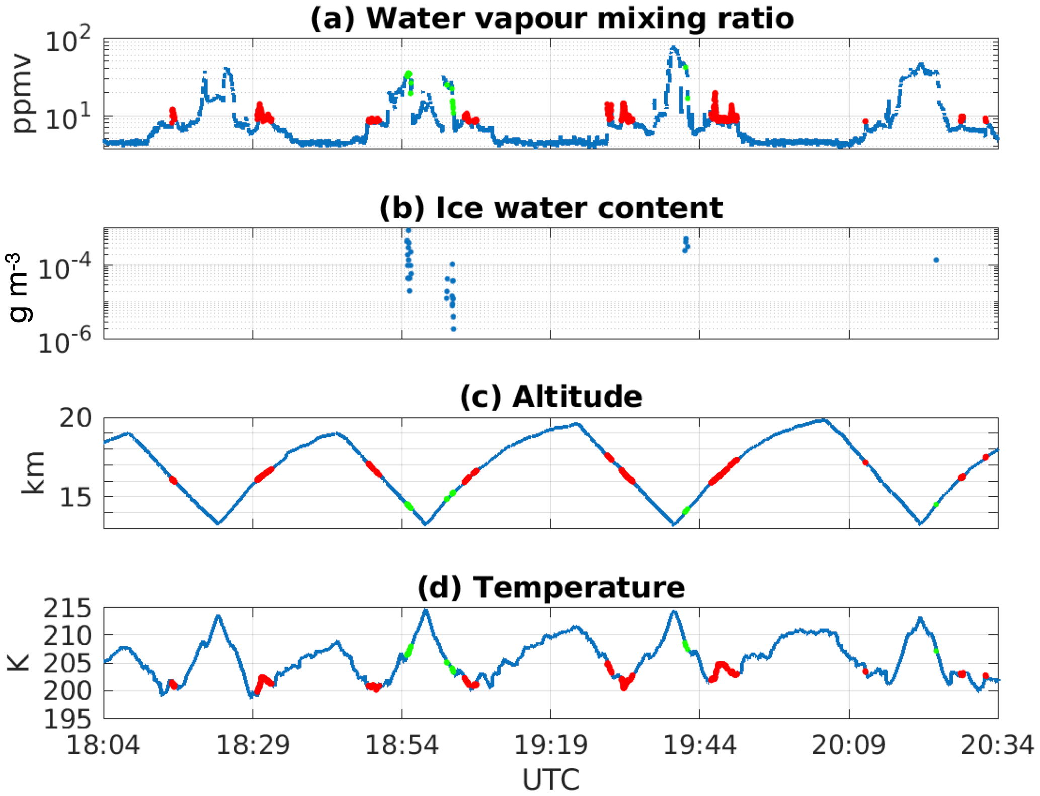
Figure 2 ER-2 aircraft observation of (a) water vapour mixing ratio in ppmv in logarithmic scale, (b) ice water content in g m⁻³, (c) altitude in km and (d) air temperature in K on 27 August 2013. The red dots highlight the measurements with pressure lower than 115 hPa (tropopause) and water vapour volume mixing ratio greater than 8 ppmv. The green dots highlight the measurements with the presence of ice.

2.3 Back-trajectory simulation

In order to include all of the different convective events potentially responsible for the moistening of the lower stratosphere captured by the aircraft measurements on 27 August 2013, we start the GEM simulations with the largest low-resolution domain (see Fig. 1) and several days earlier. Several mesoscale convective events developed on different days near the Great Lakes within this domain. To identify the source of water vapour for the aircraft-measured samples, the back trajectories of the air parcels are simulated using the trajectory model, LAGRANTO (Sprenger and Wernli, 2015), and GEM-generated wind fields. Using this technique, we find that the large water vapour anomalies observed by the aircraft in Domain B on 27 August 2013 originated from two deep convection events. The first one began at the end of 25 August and ended at the beginning of 26 August in Domain A (46 to 50^∘ N, 100 to 87.5^∘ W, ∼860 km × 445 km²), as illustrated in Fig. 1 (see below for more discussion). This convection has major contribution to the water vapour content in the lower stratosphere of Domain B. The second source is the convection that began at the end of 26 August and ended at the beginning of 27 August in Domain A. This second convection increases the water vapour content in the northern part of Domain A. This agrees with the results of Smith et al. (2017) in which the humid air parcels observed by the aircraft near 19:40 UTC (Fig. 1, northeast of Domain B) are traced back to the convection began at the end of 26 August.

3 Model results and analysis

3.1 Convective system

We first examine how well GEM simulates the general features of the deep convection events of central interest (within Domain A). Figure 3 shows the brightness temperature for the middle-infrared atmospheric window, which indicates the cloud top height, synthesized from the GEM simulations at different horizontal resolutions and observed by GOES-13 geostationary satellite (the 11.2 µm channel, Knapp et al., 2018). The synthetic radiances are calculated for the 10.2–12.2 µm spectral interval using the Rapid Radiative Transfer Model for GCMs (RRTMG, Mlawer et al., 1997; Iacono et al., 2000, 2008) with GEM-simulated atmospheric and surface properties as inputs. The target convective event simulated by the high-resolution models (2.5, 1 and 0.25 km) begins at around 18:00 UTC, 25 August. The convection is initiated a bit later in the 10 km grid spacing simulation, at around 21:30 UTC. To account for this difference, the synthetic images from model simulations are all taken at 5 h after the initiation of the convection. The 0.25 km simulation is limited to a small domain due to the limits of computational resources. Its domain is centred where the convection is initiated (48.5^∘ N, 95.5^∘ W). With an eastward movement, parts of the storm system quickly move outside of the simulation domain. We therefore do not include the 0.25 km simulation for the comparison in Fig. 3.

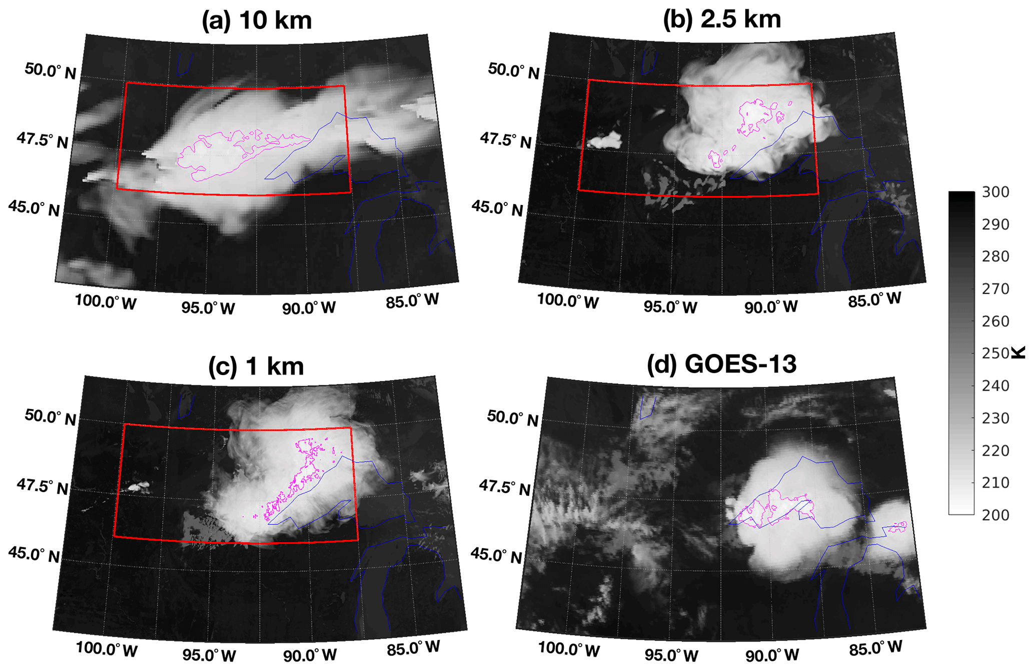
Figure 3 GEM-simulated deep convective clouds compared to satellite observation. Brightness temperatures are simulated using the RRTMG radiative transfer model, from GEM simulations at three resolutions with 10 km (02:30 UTC, 26 August), 2.5 km (23:00 UTC, 25 August) and 1 km (23:00 UTC, 25 August) grid spacing and compared to the brightness temperature of 11.2 µm channel of GOES-13 satellite (06:00 UTC, 26 August). The red rectangles mark Domain A. The magenta lines highlight the area with a brightness temperature lower than 210 K.

From Fig. 3, we can identify the location and extent of the convective system from the white-coloured areas that signify low cloud top temperatures (high cloud tops). GEM succeeds to predict a strong convective system in the area near the Great Lakes. The locations of the convection are slightly different from one simulation to another. The 10 km simulation places the convective system west of Lake Superior. The two higher-resolution simulations put the same convective system slightly northwest of Lake Superior. The satellite image shows the storm system over Lake Superior. Another difference is the horizontal extent of the anvil clouds. The two higher-resolution simulations generate anvil clouds of very similar forms to the observation. The 10 km simulation, however, generates clouds that extend in the northeast–southwest direction and covers a noticeably larger area than what is observed by the satellite. We notice that the 10 km simulation has a larger area, with the brightness temperature lower than 210 K (magenta-highlighted areas) than those in the high-resolution simulations or those in the GOES-13 images. These highlighted zones with cold cloud tops represent the intensive convective areas. For all three simulations with different horizontal grid spacing, the convective areas are all located within Domain A during the 5 h period after the initiation of convection.

In order to inter-compare the simulations at different resolutions, we perform the evaluation for Domain A, which encompasses the convective event of interest in the three simulations at 10, 2.5 and 1 km grid spacing. The time window for the evaluation is the initial 5 h of the convection development. During this time, the convection system of interest initiated, developed multiple overshooting tops and moved from the west to the east end of Domain A. At the end of the evaluation time window, the heights of overshooting tops are observed to generally decrease (not shown), which shows that the chosen window captures the primary cross-tropopause transport of water by the convective system. Due to its limited domain area, the results of the 0.25 km simulation are not included for inter-comparisons based on Domain A. Instead, the first hour of the convection event in this simulation (before the system begin to move out of the simulation domain illustrated by the green box in Fig. 1) is analyzed for comparing some aspects of the convection (see below).

3.2 Overshooting tops and gravity wave breaking

We examine the overshooting tops in the GEM simulation and especially the gravity wave breaking process that was found to primarily account for the water transport into the lower stratosphere in overshooting events. In our simulations, we find both the 1 and 0.25 km simulations generate similar structure of jumping cirrus to the previous studies (e.g., Wang et al., 2009, 2011). To illustrate the results, we show in Fig. 4 vertical cross section in Domain A at 19:46 UTC on 25 August from the 1 km simulation. In addition, two movies made from this simulation are included at https://doi.org/10.17632/8hry654mxr.2 (Qu, 2019).

Figure 4 GEM-simulated overshooting convection. The results illustrated here are taken from the 1 km simulation at 19:46 UTC, 25 August 2013: (a) temperature (colour) and potential temperature (thin white lines); (b) ice water content, in logarithmic scale; (c) water vapour mixing ratio, in ppmv; (d) vertical wind speed, in m s⁻¹; and (e) ice water content in Domain A at the level of 15.24 km at 19:46 UTC on 25 August from the 1.0 km simulation. The red line shows the location of cross section A–B.

Figure 4 shows a few key variables that highlight the impacts of overshooting tops and induced gravity wave breaking. Two overshooting tops are well identified between the longitudes of 95.94 and 95.57^∘ W by the upward-extruding isentropic lines in Fig. 4a. The temperature within the overshooting tops is noticeably colder. To the right of the overshooting tops near 95.60^∘ W, the region with overturned isentropic lines and convective instability ($\mathrm{d}\mathit{\theta }/\mathrm{d}z<\mathrm{0})$ is marked by a red circle. As found in previous studies (e.g., Wang, 2003; Wang et al., 2009, 2011), this instability develops in association with the breaking of gravity waves near the overshooting tops. The wave breaking leads to a sudden jump of air flow and transports both ice particles and water vapour upward into higher altitudes in the stratosphere, which is visible from the ice water content (IWC) and water vapour distributions in Fig. 4b and c. At the time shown in Fig. 4, the wave breaking region mentioned above is forming a jumping cirrus patch that is marked by the red arrows. Two other jumping cirrus, formed earlier, can be found near 96.10 and 95.75^∘ W, as marked by the two magenta arrows. In our simulations, we find that the jumping cirrus can extend to 2 to 3 km above the tropopause (∼14.5 km, according to the World Meteorological Organization (WMO) definition, i.e., the altitude with lapse rates Γ decreased to 2 ^∘C km⁻¹ or less). The lower stratospheric regions around the jumping cirrus are also characterized by high water vapour concentrations (up to 20 ppmv; see Fig. 4c). The water vapour plumes generated are typically 10 km ×10 km² or less in size. However, in some cases, continuously occurring overshooting produces aggregated plumes, which have a size as large as 30 km ×30 km². The continuous development of the overshooting tops, breaking gravity waves and jumping cirrus are shown by the movie in Qu (2019). Ice plumes are also formed near the areas where the gravity wave breaking happens. Two sources are found: the direction transport of ice and the formation of ice under supersaturation conditions within humid plumes. Their sizes are generally smaller than those of the water vapour plumes because ice will be completely sublimated and sedimented within a short period of time, generally within 1 h.

The cloud ice properties are different in the overshooting tops and in the thin ice plumes. At the altitude of ∼ 15.5 km (∼1 km above the tropopause) within Domain A at 19:42 UTC, 25 August, the ice water content in the overshooting tops is relatively high with values from ∼0.5 up to ∼2.8 g m⁻³. In the thin ice plumes the ice water content is generally lower than 0.1 g m⁻³. We calculated the effective radius for each solid category, e.g., ice crystals, rain, snow, graupel and hail. We find that in the overshooting cloud tops, the mass-weighted effective radius for ice increases with the ice water content from ∼300 to ∼700 µm. On the other hand, the mass-weighted effective radius for thin ice plume is usually lower than 30 µm. The area of overshooting cloud top occupies only 2.3 % of the cloudy area but contains 68 % of the total ice mass at this altitude.

We find in our simulations that the breaking of gravity waves occurs in many ways similar to the breaking of lee waves, which are formed when air flows through a mountain range. On the leeward side of the mountain, when the wave amplitude reaches a critical level, a convectively unstable region develops and consequently leads to wave breaking (Wurtele et al., 1993; Dörnbrack, 1998; Strauss et al., 2015). In the regime of gravity wave breaking, we can identify a sudden jump of the stratiform flow (Houghton and Kasahara, 1968). In its vicinity, wave energy is dissipated through turbulence which causes a strong mixing. It was found that such wave breaking occurs when the horizontal wind speed perturbation opposes the mean flow and causes stagnation, meeting a prognostic condition (Baines, 1995; Sachsperger et al., 2015):

$$\begin{array}{}\text{(1)}& \mathrm{|}{u}^{\prime }/U\mathrm{|}\mathit{⪆}\mathrm{1},\end{array}$$

where U is the mean flow speed and u^′ is the horizontal wind speed perturbation, which can be derived from the vertical wind speed perturbation w^′ using a two-dimensional incompressible mass continuity constraint:

$$\begin{array}{}\text{(2)}& \mathrm{|}\partial u^{\prime }/\partial x\mathrm{|}=\mathrm{|}\partial w^{\prime }/\partial z\mathrm{|},\end{array}$$

where x is the horizontal distance and z is the vertical height. Larger obstacles will generate larger w^′, which in turn derives larger u^′. When u^′ is large enough to satisfy the condition in Eq. (1), wave breaking occurs.

Analogies can be drawn to the gravity wave breaking near the overshooting tops. The overshooting tops carry air mass of different horizontal velocity into the lower stratosphere and act to block the pre-existing horizontal flow there (westerlies with speeds ranging from 5 to 25 m s⁻¹ at different altitudes). The obstructed stratified flow in the lower stratosphere is forced to pass around the overshooting tops, creating a similar situation to air flow passing a mountain range and inducing gravity waves.

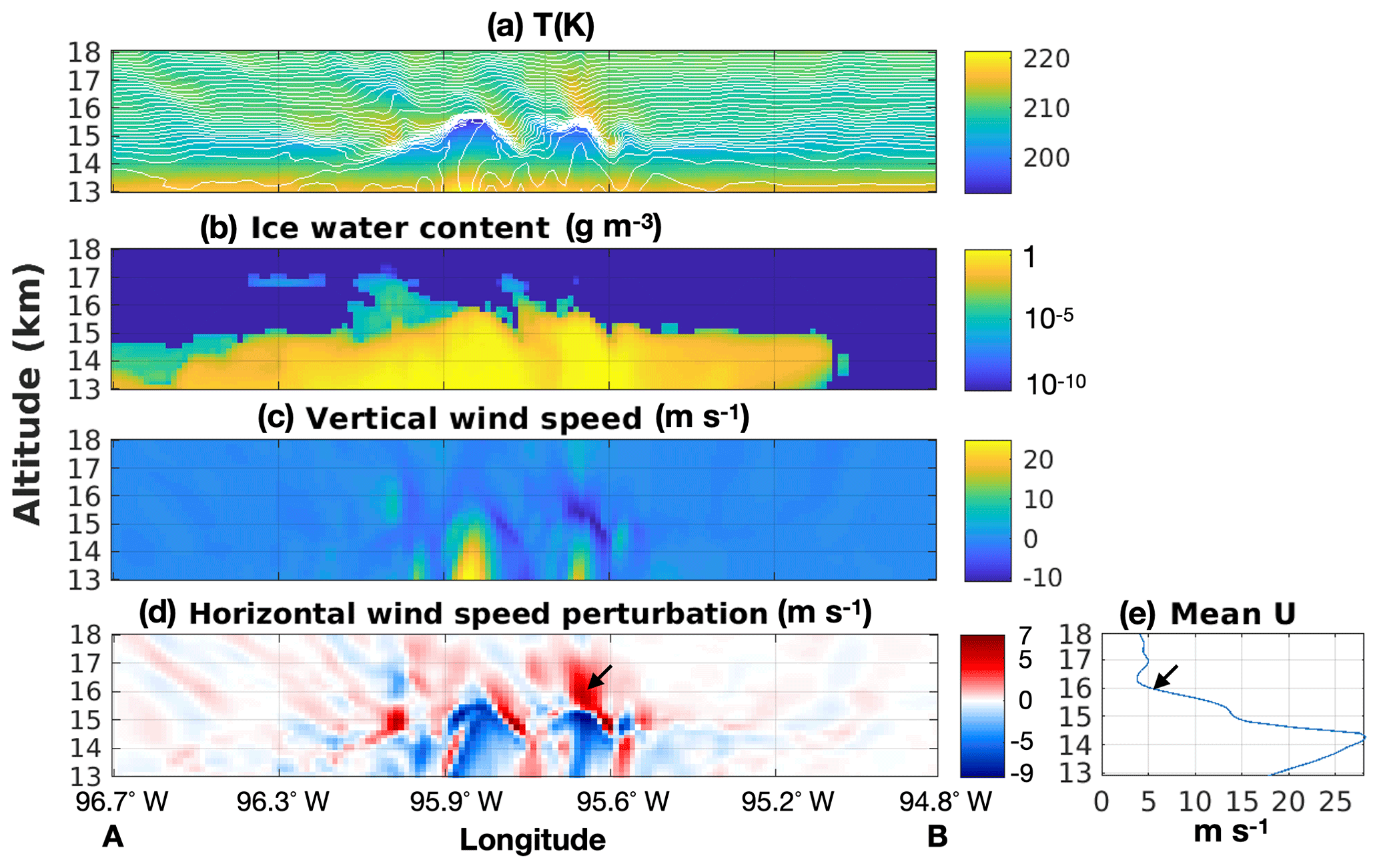
Figure 5 Cross section as shown in Fig. 4 but for 19:42 UTC, 25 August 2013: (a) temperature (colour) and potential temperature (thin white lines); (b) ice water content, in logarithmic scale; (c) vertical wind speed, in m s⁻¹; (d) horizontal wind speed perturbation based on Eq. (2), in m s⁻¹; and (e) the mean horizontal west wind speed.

Figure 5 shows several key variables for the same cross section shown in Fig. 4 but 4 min earlier (19:42 UTC), when the condition of gravity wave breaking (Eq. 1) is satisfied. At this moment before the formation of jumping cirrus, the overshooting cloud top near 95.6^∘ W is falling after reaching its maximal altitude with a speed of $\sim -\mathrm{10}$ m s⁻¹ (Fig. 5c, dark blue area between the altitude of 15 and 16 km). This downward movement will eventually bring the majority of overshot ice and vapour back to the equilibrium level below the tropopause. The falling of the overshooting top generates a strong vertical wind speed gradient (right-hand side of Eq. 2) just above the overshooting top near the altitude of 16 km. Using Eq. 2, we calculated the corresponding horizontal wind speed perturbation (u^′) shown in Fig. 5d. An area with strong u^′ with maximal value of ∼6 m s⁻¹ can be found above the falling overshooting cloud top, as shown by the black arrow. This value is of the same range as the background horizontal wind speed in the west–east orientation at the altitude of 16 km (∼5 m s⁻¹ on Fig. 5e). The condition in Eq. (1) is then satisfied, which leads to the stagnation of air flow and the breaking of gravity waves. The breaking of the gravity wave further formed the jumping cirrus shown in Fig. 4 (red arrow). In this process, a significant amount of ice and water vapour is transported irreversibly into the lower stratosphere instead of falling back to the equilibrium level.

We emphasize the “irreversibility” of the vertical upward transport during the gravity wave breaking event. In case of a non-breaking gravity wave, the ascending air will later descend after reaching the wave ridge. In this case, the upward transport is “reversible”. In addition, there is weaker turbulent mixing to bring up the moister air below because the wave energy is less transferred to turbulence but is propagated away. In the case of gravity wave breaking, a sudden jump of air flow occurs. The wave energy is dissipated through turbulence in the vicinity of the jump which enhances the mixing and the transport of water vapour and ice from the upper troposphere to the lower stratosphere.

The occurrence of gravity wave breaking depends on the intensity of the overshooting strength. As shown in Eq. (2), the magnitude of the horizontal speed perturbation is linked to the vertical wind speed perturbation, which in this case is related to the overshooting strength. This is in agreement with the finding of Dauhut et al. (2018) that stronger overshooting tops favour wave breaking and thus facilitate more vertical water transport.

We find in our simulations that the overshooting tops and wave breaking are frequently observed in the 0.25 and 1 km simulations, with the breaking waves and jumping cirrus of typical horizontal sizes of 2 to 3 km. These phenomena are visible in the 2.5 km simulation, although with less frequency and intensity, and are not found in the 10 km simulation because the grid size cannot resolve the process.

3.3 Humidity and ice field

We further examine the water vapour fields simulated by GEM at different horizontal grid spacing. Figure 6a and b show the mean vertical profiles of water vapour volume mixing ratio and temperature within the above-defined Domain A and 5 h time window. All the simulations show irregular moisture profiles near 16 km, where the vertical trend of the humidity profiles bends and produces “bumps” (elevated water vapour contents) above the tropopause (indicated by the circles in Fig. 6; hereafter the tropopause is defined by the altitude where the mean lapse rate Γ within Domain A and 5 h time window decreased to 2 ^∘C km⁻¹or less). Surprisingly, the low-resolution (10 km) simulation predicts the highest water vapour content in a large part of the UTLS. This is interesting because, as described above, the overshooting tops and the gravity wave breaking processes are only resolved in the higher-resolution simulations, which causes vertical water transport and explains the moistened lower stratosphere in these simulations. The moister lower stratosphere in the 10 km simulation (compared to the 1 and 2.5 km simulations) warrants further investigation. In this subsection, we first use satellite remote sensing and aircraft in situ observations to validate the vertical humidity profiles, to find out which simulation better approximates the reality and then, in the following subsection, we diagnose the causes of the identified model biases.

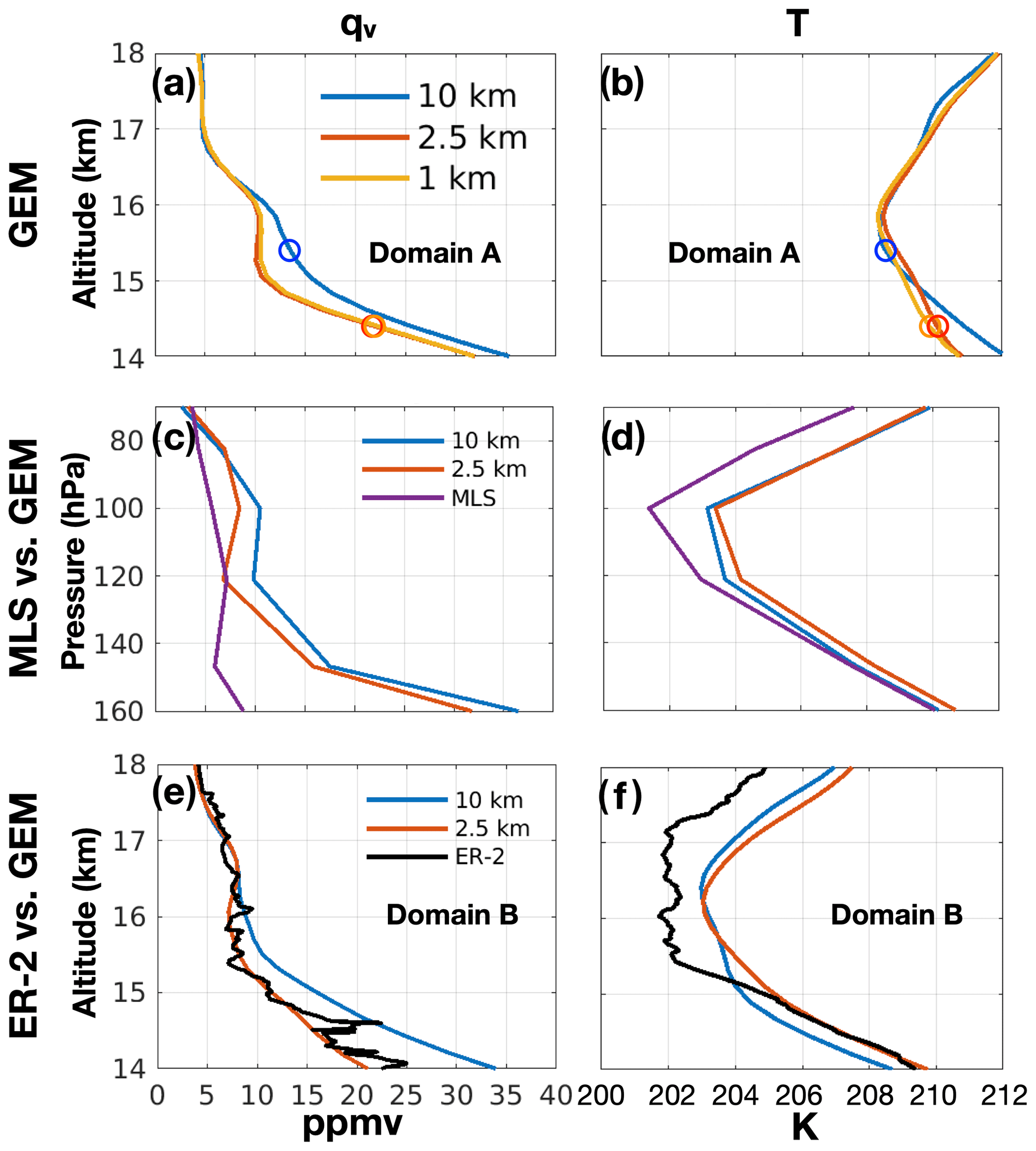
Figure 6 (a, b) The mean profiles of water vapour volume mixing ratio (q_v) and temperature (T) for Domain A during the 5 h period. The circles indicate the positions of the tropopause (mean Γ<2 ^∘C km⁻¹). (c, d) Mean profiles (q_v and T) after applying averaging kernels of MLS to the GEM 2.5 km and 10 km simulations (100 km ×100 km areas centred on five MLS footprints) and MLS profiles. (e, f) The vertical profiles (q_v and T) within Domain B for GEM 10 km and 2.5 km simulations and for ER-2 aircraft in situ observations.

It is challenging to observe the humidity at the levels near tropopause. Nadir-view satellite remote sensing instruments, such as the Atmospheric Infrared Sounder (AIRS) on board the NASA Aqua satellite, usually cannot accurately measure the low water vapour concentrations in the lower stratosphere (e.g., Divakarla et al., 2006), although attempts have been made to improve the retrieval under special circumstance (e.g., Feng and Huang, 2018). Limb-view sounders such as the Microwave Limb Sounder (MLS) on board the Aura satellite have higher sensitivity and provide measurements of water vapour content in the UTLS, although biases have also been noted in these datasets. These biases might be caused, among many others, by the averaging kernels of limb sounders which smear out the strong vertical gradient in water vapour at the tropopause (Hegglin et al., 2013). For instance, an underestimation of water vapour with mean bias up to −25 % and biases for individual case up to −85 % between 100 and 300 hPa were reported for the MLS retrieval (Read et al., 2007; Vömel et al., 2007; Livesey et al., 2018). It is important to bear in mind the uncertainty in the satellite data when comparing the simulations with the observations.

Figure 6c and d show the comparisons between the GEM simulations after applying averaging kernels of MLS and MLS retrievals (v4.2). Because of the scarcity of the co-located satellite data and the aforementioned mismatch in time and location of the simulated convective system, we conduct the comparison with respect to area averages rather than individual samples. The MLS measurements used here include five MLS footprints located between 38–45^∘ N and 95–93^∘ W, taken on 26 August 2013 at around 19:00 UTC, about 15 h after the dissipation of the convection system (Fig. 7, red diamonds). We applied the averaging kernel of MLS on the mean profiles of GEM-simulated humidity and temperature within the 100 km ×100 km regions centred on the MLS footprints. The comparison here suggests that both model simulations give higher estimations of water vapour content in the UTLS compared to MLS retrievals, although the higher-resolution simulation better approximates the satellite observations. It is also found that GEM slightly overestimated the temperature compared to MLS retrievals. This suggests that warmer temperatures in comparison to MLS could lead to slower ice crystal growth and thus less dehydration and higher gas-phase water. The spatio-temporal errors of the model simulation, e.g., shifted convection location or time, might also contribute to the discrepancies between the GEM and MLS profiles. Furthermore, the lower value of water vapour content from MLS near the level of 160 hPa may be subject to the aforementioned negative bias in the MLS data.

Figure 7 Back trajectories of air parcels. All the trajectories, in black lines, are initialized in Domain B at 15.5 km altitude and 19:40 UTC, 27 August. The circles indicate the initial locations of each back trajectory. The grey line illustrates the ER-2 aircraft flight path (in clockwise direction). The background image shows the water vapour content in ppmv at this level from the 2.5 km simulation. The red line highlights the back trajectory of one air parcel from its initial location in Domain B to its location in Domain A at around 23:00 UTC, 25 August 2013, when the overshooting convection occurred. The evolution of the properties of this air parcel are shown in Fig. 8. The red diamonds indicate the centre of five MLS footprints on 26 August.

High-accuracy hygrometers on-board high-altitude aircrafts provide benchmark water vapour measurements, although the temporal and spatial coverage of the aircraft data are limited. On 27 August 2013, the ER-2 aircraft deployed in the SEAC⁴RS field campaign obtained UTLS water vapour measurements located to the southwest of the Great Lakes, as shown in Fig. 1. Using back-trajectory calculations we find that the measured air samples in Domain B are in the downwind direction of our studied convective system in Domain A. For the back-trajectory calculations we use the wind field simulated by GEM at 2.5 km grid spacing. It is used to trace air parcels at 56 locations on 8 vertical levels between 14 and 17.5 km and 500 m intervals. Figure 7 shows the back trajectories of 16 selected air parcels starting at the altitude of 15.5 km and at the time of 19:40 UTC, 27 August, when the aircraft measurements were taken. Through the back trajectories, we find that most of the air parcels in Domain B previously passed through Domain A where the convective system analyzed above developed. The high moisture content samples located in the southwest corner of Domain B are especially found to be moistened by the overshooting convection. Figure 8 illustrates the evolution of a few properties of one of these convectively moistened air parcels located in the southwest corner of Domain B at the tropopause altitude of 15.5 km. Similar results are found for the other altitudes above (not shown). The results here establish a connection between Domain A and Domain B for the lower stratosphere. It is particularly clear that the ER-2-aircraft-measured UTLS air samples characterize the moistening effects of the overshooting convection that occurred earlier (and were analyzed above) in Domain A.

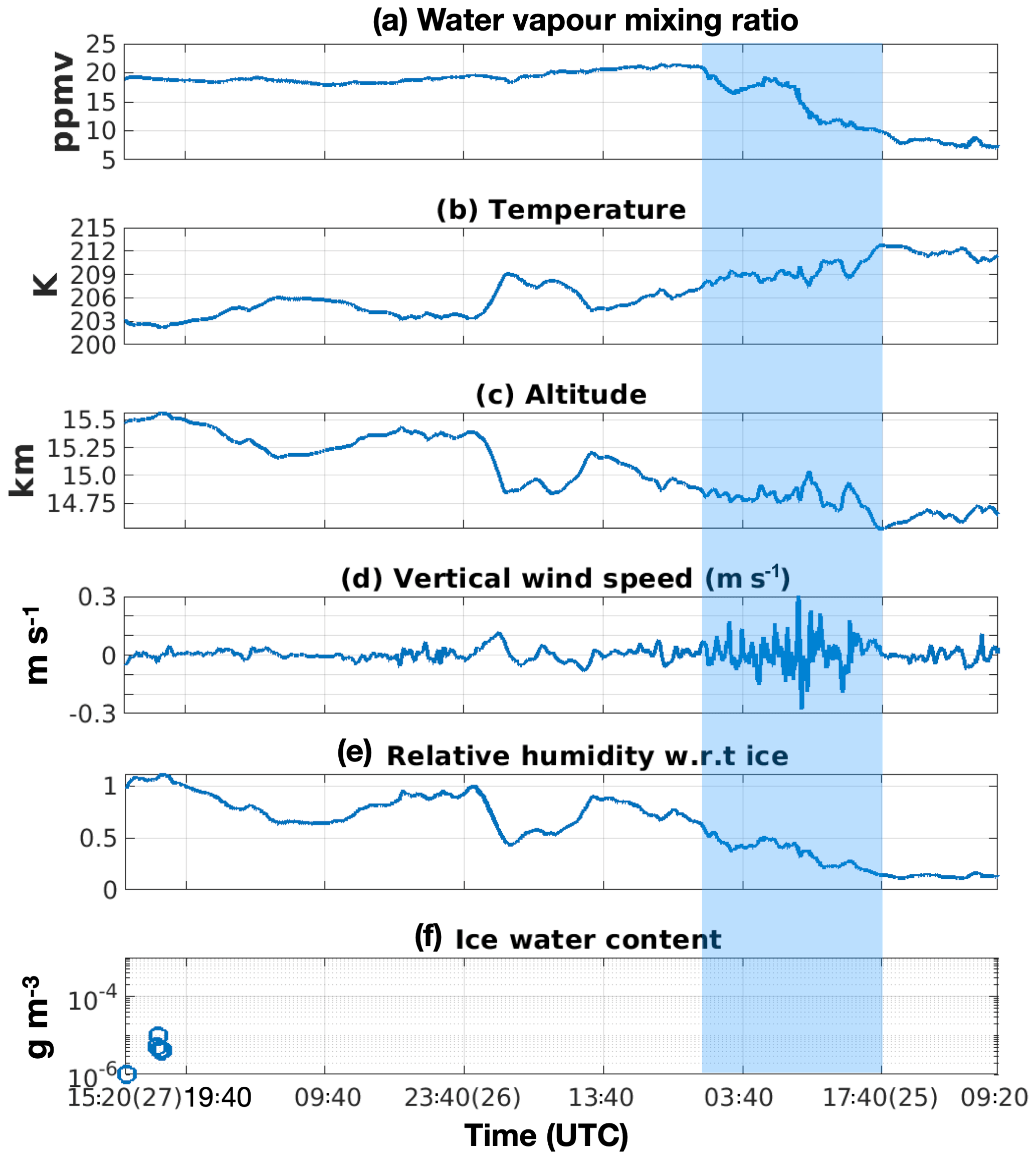
Figure 8 The changes of the properties of a tracked air parcel (red circle highlighted in Fig. 7) along its back and forward trajectory. The beginning time of the back and forward tracing is 19:40 UTC, 27 August. Highlighted in the rectangular shaded area is the encountering of the air parcel with the overshooting convections in Domain A at around 22:40 UTC, 25 August, which is shown by fast-rising water vapour concentration, decrease in temperature, rise in altitude and sudden changes in vertical wind speeds.

One particular note for Fig. 8 is the formation of ice shortly after 19:40 UTC, 27 August, when the humid air parcel slowly ascends with decreasing temperature and increasing relative humidity with regard to ice. At these altitudes, the ice water content is relatively low ($\sim \mathrm{1}\times {\mathrm{10}}^{-\mathrm{5}}$ g m⁻³). The ice particles will gradually fall to a lower altitude and eventually be sublimated again. This process will partly dehydrate the upper layer of the atmosphere where the ice is forming and later hydrate the lower atmospheric layer through ice sublimation. However, this dehydration has a minor impact on the air parcels above the tropopause. We observe that the water vapour mixing ratio of the air parcel at the 15.5 km altitude (i.e., the upper layer) increased slightly after 19:40 UTC (Fig. 8a). This might be the result of the mixing with the adjacent air in the northeast side of the parcel, which is more humid (pointed by the black arrow in Fig. 7). As ice formation in Domain B is found to have limited impact on the humidity field above the tropopause, our interpretation of the stratospheric water vapour injected in Domain A by linking it to the water vapour simulated and observed in Domain B is therefore not affected in a significant way.

For the atmospheric layer under the tropopause between the altitude of 13.5 and 14.5 km, the horizontal wind speed increases significantly. The back-tracking results show that the humidity and ice field in the northern part of Domain B are linked to the convection initiated at the beginning of 27 August in Domain A. The locations of ice water content in Domain B from the simulation partly agree with what are observed by the aircraft in Fig. 2b. Based on the back tracing results, we noticed that the ice in Domain B is not originally formed during the convection, but later during the slow ascent of the humid air parcel. This is similar to the dehydration process discussed above but at a lower altitude below the tropopause. The ice formed at this lower altitude is more abundant (on the order of $\mathrm{1}\times {\mathrm{10}}^{-\mathrm{3}}$ g m⁻³). The impact of dehydration (via ice formation and falling) at this level is more significant, which can be seen in Fig. SI.3 (Qu, 2019) near 15:40 UTC with an amplitude of about 20 ppmv. The readers are referred to Qu (2019) for more discussions on this topic (Figs. SI.2 and SI.3).

Given the variability of water vapour in Domain B, as shown in Fig. 7, and possible errors in the location and time of GEM-simulated water vapour features, it would not be meaningful to compare the aircraft measurements with GEM simulations at exactly matched locations and times. Instead, we compare the mean vertical profiles averaged for Domain B between the aircraft observations and GEM simulations in Fig. 6e and f. We note that only the 10 and 2.5 km simulations cover Domain B where aircraft data are available (see Fig. 1). We observe a slight temperature bias from both model simulations of ∼2 K above the tropopause level at 15.5 km (Fig. 6f). For water vapour content, Fig. 6e shows that the 2.5 km model predicts the aircraft measurements well, which indicates noticeable moistening around the altitude of 16.5 km. Although it also captures this moistening feature, the 10 km simulation generally overestimates the water vapour contents in the UTLS region. This is consistent with the comparison made in Domain A against satellite measurements (see Fig. 6c and discussions above). This noticeable moist bias in the 10 km simulation warrants an investigation of its cause. As the convective parameterization is turned on at this resolution, both resolved vertical air motions and parameterized vertical transport (via the KFC scheme) potentially account for the convective moistening in GEM. This is similar to the simulations of GCMs, which also generally overestimate the UTLS humidity. In the next subsection, we diagnose how an overly moist UTLS occurred in the coarse-resolution simulation.

3.4 Budget analysis

We diagnose the water vapour transported across the tropopause into the lower stratosphere in the GEM simulations. The water budget is calculated for the rectangular box surrounded by a given lower boundary (e.g., tropopause) and model top (∼30 km), as well as the four lateral facets of Domain A. Using the wind, water vapour and tendency fields generated by GEM, we calculate the contributions to the change in total water vapour in the stratospheric box due to vertical advection of water vapour, as well as the sublimation of ice.

First, we use the Reynolds decomposition (Eqs. 3–5) to diagnose the direct vertical transport (vertical advection) of water vapour for the two high-resolution simulations (1 and 2.5 km grid spacing). For the 10 km grid spacing simulation, the vertical advection is composed of two parts: the grid-scale advection, which is solved explicitly, and the parameterized sub-grid-scale transport (tendency on water vapour due to KFC), which makes this case not suitable for Reynolds decomposition.

$$\begin{array}{}\text{(3)}& {\displaystyle }w\left(xyt\right)=\stackrel{\mathrm{‾}}{w(x,y)}+w(xyt{)}^{\prime }\text{(4)}& {\displaystyle }q\left(xyt\right)=\stackrel{\mathrm{‾}}{q(x,y)}+q(xyt{)}^{\prime }\text{(5)}& {\displaystyle }\begin{array}{rl}\sum _{nt=\mathrm{1}}^{nt=N}& \sum _{ns=\mathrm{1}}^{ns=M}\mathit{\delta }t\mathit{\delta }sw(x,y,t)q(x,y,t)\\ & =N\mathit{\delta }t\sum _{ns=\mathrm{1}}^{ns=M}\mathit{\delta }s\stackrel{\mathrm{‾}}{w(x,y)}\stackrel{\mathrm{‾}}{q(x,y)}\\ & +\sum _{n=\mathrm{1}}^{n=N}\sum _{ns=\mathrm{1}}^{ns=M}\mathit{\delta }t\mathit{\delta }sw(x,y,t{)}^{\prime }q(x,y,t{)}^{\prime }\\ & +\sum _{n=\mathrm{1}}^{n=N}\sum _{ns=\mathrm{1}}^{ns=M}\mathit{\delta }t\mathit{\delta }s\stackrel{\mathrm{‾}}{w(x,y)}q(x,y,t{)}^{\prime }\\ & +\sum _{n=\mathrm{1}}^{n=N}\sum _{ns=\mathrm{1}}^{ns=M}\mathit{\delta }t\mathit{\delta }sw(x,y,t{)}^{\prime }\stackrel{\mathrm{‾}}{q(x,y)}\end{array}\end{array}$$

We decompose the vertical wind speed w and humidity q into the time-averaged terms and fluctuation terms, as shown in Eqs. (3) and (4), where x and y represent the coordinates of longitude and latitude and t represents the time. The integrated product of w and q for the evaluation domain and time is shown in the Eq. (5), where N is the total number of time steps of the simulation during the evaluation window, M is the total number of horizontal grid boxes in Domain A, δt is the length of each time step and δs is the horizontal surface of a given model grid box.

Applying Eq. (5) at the tropopause level in Domain A (mean Γ<2 ^∘C km⁻¹), we obtain a first-order approximation of the vertical transport of water vapour through the tropopause. Among the four terms on the right side of the Eq. (5), the last two terms are negligible. The first term on the right side of the equation measures the transport of water vapour through tropopause by the mean updraft (or downdraft). The second term on the right side of the equation includes transport by “eddies” generated by wave breaking. Through the decomposition for the 1 km simulation, we find that the first term represents 39 % of the total vertical transport and the second term represents 59 %, which highlights the important role of wave breaking. With the decrease in model's horizontal resolution, the weight of the eddy term decreases to 29 % for the 2.5 km simulation. This suggests that the importance of wave breaking in direct vertical transport of water vapour decreases with the model resolution.

Secondly, we calculate the total transport of water vapour and the contributions from direct transport and ice sublimation for each simulation. The comparison between the high-resolution simulations and the 10 km simulation is less straightforward because their tropopause heights are different (Fig. 6a and b). We therefore calculated the water vapour change due to the vertical advection and ice sublimation and vapour deposition with different altitude levels as the lower boundary from 14 to 16 km. These results are shown in Fig. 9.

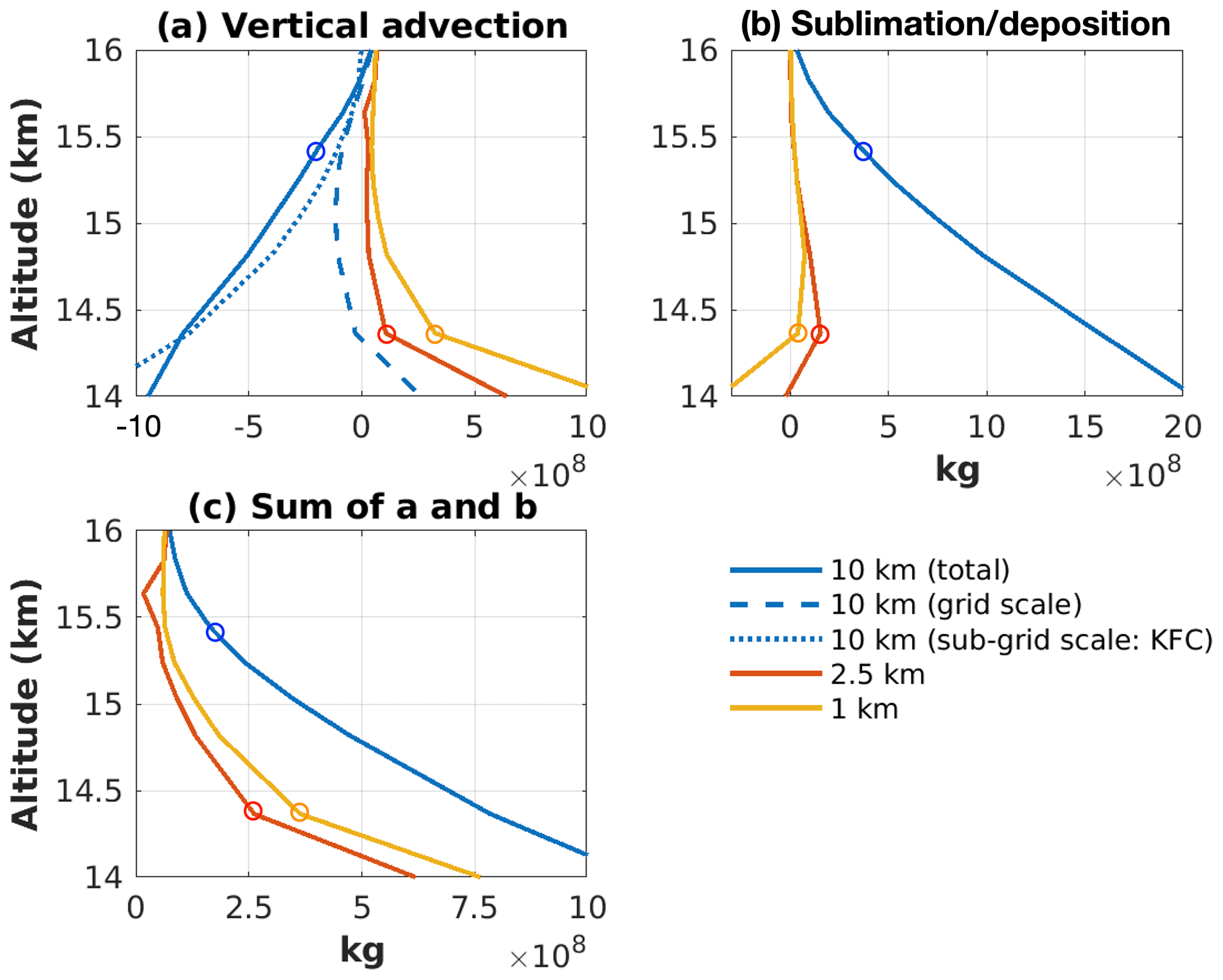
Figure 9 Change of water vapour in Domain A during the 5 h evaluation period with different altitude levels as the lower boundary. The circles represent the height of tropopause (mean Γ<2 ^∘C km⁻¹).

The vertical advection simulated by the high-resolution models is relatively constant from 14.5 to 16 km altitude with positive values (upward transport, Fig. 9a). This upward advection is linked to the gravity wave breaking (see discussion in Sect. 3.2), which makes the stratospheric air flow jump by about 2 km upward and transports humidity into the stratosphere. The vertical advection in the 1 km simulation is generally stronger than that of 2.5 km simulation due to the more important role of wave breaking. This is in agreement with the results from Reynolds decomposition.

It is not a surprise that the higher-resolution NWP models tend to produce stronger direct vertical transports across the tropopause because, as shown in Sect. 3.1, the transport is closely related to the strength of overshooting and the breaking of the gravity waves. Similar to what was found by Weisman and Klemp (1982), we find in our GEM simulations that the simulated maximal vertical wind speed is inversely proportional to the horizontal grid spacing of the NWP model. The stronger vertical wind speed in the convection updraft leads to higher overshooting cloud top. In our cases with high-resolution simulation, the maximum cloud top altitude is 16.64 and 16.96 km for 2.5 and 1.0 km simulation, respectively. We find that the stronger overshooting wind speed in the higher-resolution simulations leads to favourable conditions for gravity wave breaking (see the discussions in Sect. 3.1) and thus more direct vertical transport. This agrees with Dauhut et al. (2018). In total, the direct vertical transport of water vapour contributes to 40 % of the total transport at the tropopause level for the 2.5 km simulation and makes up to 89 % for the 1.0 km simulation.

The total vertical advection from 10 km simulation is different from those of the two high-resolution simulations. It can be decomposed into two parts: the grid-scale explicit advection (dashed blue line in Fig. 9a) and the sub-grid-scale advection by KFC (dotted blue line in Fig. 9a). The grid-scale vertical advection of 10 km simulation is positive below the altitude of 14.3 km. It turns to negative values from 14.4 km. One of the reasons for these negative values may be the lack of representation of gravity wave breaking. Another reason is possibly the large-scale circulation induced by the convection. In the convective area, the air transported to the level above 14 km is relatively dry and cold, whereas the descending areas surrounding the convective zone are moister due to the sublimation of the ice. The sub-grid-scale advection is strongly negative at lower altitude. In KFC, this downward transport comes from the effect of compensating subsidence outside of the convective updrafts. This strong downward transport gradually reduces to zero near the tropopause.

We find large discrepancies in the contribution of ice sublimation throughout the UTLS region between the high-resolution simulations (1 and 2.5 km) and the 10 km simulations. Ice sublimation (hydration) and vapour deposition on ice (dehydration) are two opposing microphysical processes competing for a dynamical balance. Hereafter, we use sublimation to denote the combined effect of these two processes. The positive value signifies that the ice sublimation is faster than the vapour deposition, and the negative value signifies the opposite. In this study, the value of sublimation includes all the ice-phase categories. For the two high-resolution simulations, the contribution of ice sublimation reaches its maximal positive value near the altitude of 14.5 km. Toward higher altitudes, the contribution of ice sublimation decreases gradually to a small value. To focus on the tropopause level, ice sublimation has a non-negligible contribution to the total transport of water vapour for the 1 km simulation (11 %) and a larger contribution for the 2.5 km simulation (60 %). For the 10 km simulation, the mean ice sublimation rate is large and always positive. Ice sublimation is therefore the primary source of moistening of the UTLS region above the altitude of 14 km. Vertical advection does not contribute to the moistening of the UTLS region but transports a significant part of water vapour back to lower altitudes. Overall, the contribution from both processes generate a strong moistening of the UTLS region for the 10 km simulation (Fig. 9c).

An additional comparison including the 0.25 km simulation for a smaller domain (see Fig. 1) and shorter period (1 h) corroborates the above finding that the simulation tends to have a larger contribution from advection and less contribution from sublimation as the resolution increases (see Fig. SI.1 in Qu, 2019).

It is, however, interesting that compared to the high-resolution simulations, the sublimation-induced lower stratospheric moistening is stronger in the lower-resolution simulations (10 km grid spacing), as shown by Fig. 9b. We find that this higher sublimation rate may be attributed to the following factors: first, more abundant ice particles in the lower stratosphere in the 10 km simulation, as shown by Fig. 10. The cause of this higher mean ice water content may be due to the lack of the parameterization of downward transport to bring the ice within the overshooting cloud tops back into the upper troposphere in the KFC deep convection scheme. In this scheme, the ice transported into the lower stratosphere by the parameterized updrafts will be distributed uniformly into the 10 km ×10 km² model grid box. The ice will then be passed into the MY2 microphysical scheme in the hydrometeor “ice” category. Part of these ice particles will eventually be transformed through aggregation or diffusional growth into other larger hydrometeors such as “snow”. But all of these solid hydrometeors can only fall back into the upper troposphere through gravitational sedimentation. In reality, as evident from the high-resolution simulations here, the majority of ice transported into lower stratosphere within the overshooting cloud tops will be brought back to troposphere when the overshooting tops fall back to the equilibrium level. This suggests that the simple entrainment–detrainment model in KFC might not represent the complexity of the different mechanisms well near the tropopause level.

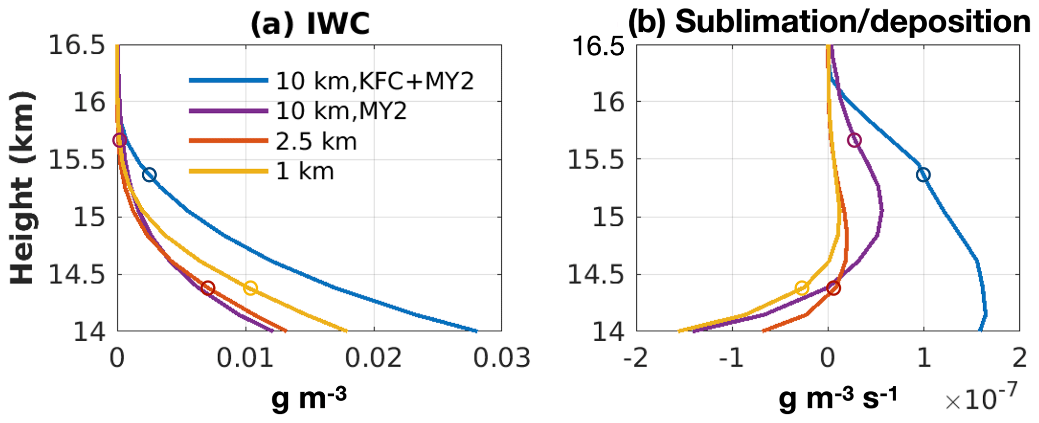
Figure 10 Mean profiles between 14 km and 16.5 km within Domain A and the evaluation time window (5 h): (a) ice water content, (b) ice sublimation and vapour deposition tendency. The circles indicate the position of tropopause (mean Γ<2 ^∘C km⁻¹).

A separate test run with 10 km model grid spacing without the KFC scheme has been performed and shows that the ice water content at the UTLS region above the altitude of 14 km is very close to the 2.5 km simulation (Fig. 10a, purple line). These results suggest that the overestimation of ice is partly due to the use of the deep convection parameterization. With the reduction of ice in the test run, we find that the mean ice sublimation tendency is largely reduced (blue line and purple line in Fig. 10b). However, with similar amount of ice in the UTLS, the 10 km simulation without KFC still shows a higher ice sublimation rate above the altitude of 14.5 km compared with the two high-resolution simulations.

This second reason leading to stronger moistening of the lower stratosphere in the coarse-resolution (10 km) simulation is due to the sublimation efficiency of ice. We find that the ice transported into lower stratosphere is largely sublimated into water vapour in the 10 km simulation and is much lower for the higher-resolution simulations. The amount of ice transported across the tropopause in the 1 and 2.5 km simulations is similar, i.e., 2.3 and 2.6×10⁹ kg, respectively, out of which only 2 % and 6 % are sublimated. In contrast, in the 10 km simulation, the vertically transported ice across a similar altitude (∼14.5 km) is 3.9×10⁹ kg and 21 % sublimated. If evaluated at the tropopause determined from the 10 km simulation (∼15.5 km, higher than the tropopause in the higher-resolution simulations), 75 % of the 4.8×10⁸ kg ice is sublimated in the 10 km simulation. In summary, the coarse-resolution simulation strongly overestimates the fraction of ice that is sublimated in the lower stratosphere compared with higher-resolution experiments.

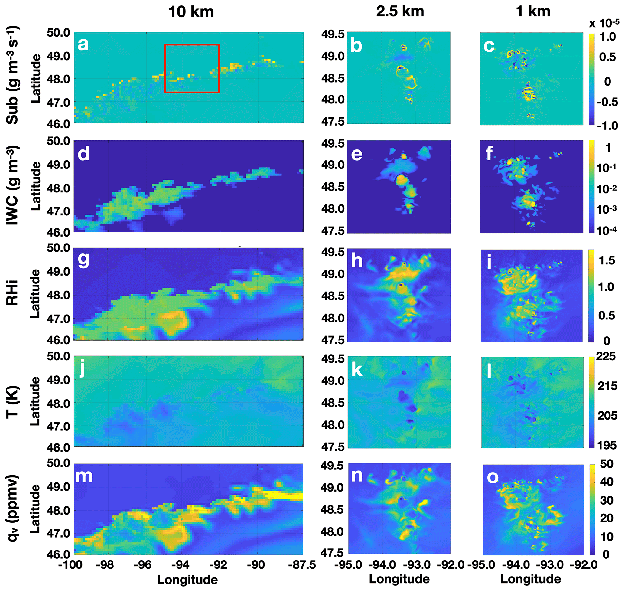
Figure 11 Distribution of a few variables in Domain A during overshooting. The results are taken from one instance, i.e., 23:25 UTC, 25 August 2013, and one vertical level of ∼15.36 km (above the tropopause). Shown in the three columns are the simulations at 10, 2.5 and 1 km horizontal grid spacing, respectively. The area shown for the 2.5 and 1 km simulations corresponds to the red rectangle in the first image. Short names for each row are used for notation: Sub, sublimation; IWC, ice water content; RH, relative humidity with regard to ice; T, temperature; and q_v, water vapour volume mixing ratio.

What leads to the drastically different ice sublimation processes in the coarse-resolution simulation? We find that one important factor influencing ice sublimation efficiency in the lower stratosphere is the spatial distribution of ice. Figure 11 shows the ice sublimation rates, IWC distributions and a few related fields from the GEM simulations at different resolutions at the level of ∼15.36 km in Domain A on 23:25 UTC, 25 August 2013. From Fig. 11a, we can identify that the 10 km simulation is populated with many pixels with high sublimation tendency (in yellow) corresponding to the edges of convective cloud areas. These areas are in-between the supersaturated air (relative humidity over ice ∼1.08) within the convection clouds and the surrounding dry mid-latitude lower stratospheric air (Fig. 11d, g). The ice sublimation rates in the higher-resolution simulations are very different. In these higher-resolution cases, the areas loaded with ice are much smaller than those in the 10 km simulation and are of much higher spatial heterogeneity. The majority of the ice is concentrated in very limited areas (Fig. 11e and f) with low temperature (Fig. 11k and l) and high relative humidity (Fig. 11h and i), corresponding to the locations of the overshooting tops. That is, the majority of ice is “trapped” in the overshooting tops. As shown by Fig. 12, this trapping effect is also shown by the distributions of ice with respect to temperature (Fig. 12a) and relative humidity (Fig. 12b), respectively, calculated by summing up the mass of ice in the grid boxes whose temperature or relative humidity values fall within each specific interval and then dividing it by the total mass of ice in the whole domain. We find that the majority of ice of the two high-resolution simulations are trapped in cold temperatures between 195 and 201 K and high relative humidity inside the overshooting tops. The horizontal extent of the areas with high ice water content is thus small. The trapped ice therefore has less contact surface with the surrounding drier stratospheric air. This factor significantly limits the ice sublimation rate in the higher-resolution simulations. In contrast, in the 10 km simulation the ice is not trapped in the cold overshooting tops but distributed over larger areas with warmer temperatures (>201 K). This leads to a significantly larger contact area with dry air and higher sublimation.

Figure 12 Distribution of ice with respect to (a) temperature and (b) relative humidity. The results are based on the variables in Domain A as shown in Fig. 11. The temperature and relative humidity intervals are 1 K and 1 %, respectively. The mass fraction value at each temperature or relative humidity interval is calculated by summing up the mass of ice in the grid boxes wherein temperature or relative humidity values fall within the specific interval and then dividing by the total mass of ice in the whole domain.

4 Conclusions and discussions

In this study we use the GEM model of ECCC to reproduce a mid-latitude lower stratospheric moistening event over North America near the Great Lakes during 25–26 August 2013. Simulations are conducted with a set of nested domains at increasing resolutions from 10 to 0.25 km grid spacing. Satellite remote sensing data from MLS as well as aircraft in situ observations from the SEAC⁴RS campaign are used to evaluate model simulations complemented with trajectory simulations to associate those observations with model forecasts over specific regions. Comparisons conducted here suggest that while the higher-resolution simulations approximate the observed water vapour fields well in the UTLS region after the deep convective events, the coarse-resolution simulation simulates a substantially moister UTLS.

By performing an intercomparison of simulations using different horizontal resolutions, we find that the high-resolution simulations (with grid spacing dx≤1 km) can properly resolve the key dynamical features of the overshooting convection, including the overshooting tops, the gravity wave breaking process and the visible jumping cirrus phenomenon. The overshooting convection may significantly elevate the water contents (both vapour and ice) up to 1–2 km above the tropopause. The size of the high-concentration water vapour plumes is typically less than 10 km, although they can aggregate to sizes greater than 30 km. Coarse-resolution simulations (dx≥10 km) cannot resolve these features, although a moister UTLS region results from the parameterized deep convection and associated water transport.

A lower stratospheric water budget has been performed to quantify the contributions of different processes. It shows that vertical advection of water vapour is one main contributor to the lower stratospheric moistening in the overshooting events. In the high-resolution simulations (0.25 and 1 km) where the gravity wave breaking process is well simulated, eddies resulting from wave breaking are found to mainly account for the direct vertical transport of water vapour into the lower stratosphere. This transport mechanism is largely dependent on the strength of overshooting (updraft speed), with higher-resolution simulations generating stronger updrafts, which enhance overall the transport of water vapour into the stratosphere.

Another important source of water vapour in the lower stratosphere is ice sublimation. The comparisons conducted in this study show that the 10 km simulation has a considerably higher ice sublimation rate. One of the possible reasons is that the KFC convective scheme that is used in this simulation brings more ice into the UTLS region which enhances the production of water vapour through the ice sublimation process. The cause of this overproduction of ice is likely associated with the lack of downward transport of ice that is observed after the overshooting cloud tops reach their maximal height in the lower stratosphere. The simple entrainment–detrainment model used in KFC scheme may not represent the complex processes near and above tropopause well during the convective event. One solution is to add an element in the KFC scheme to take this downward transport above the tropopause into account. Another solution is to increase the ice particle size in the UTLS so that the ice can sediment faster and hence reduce the ice water content at these levels. Another possible reason why the 10 km model has a higher sublimation rate is the high ice sublimation efficiency. This high efficiency is due to the different distribution of ice water contents compared to the those of high-resolution models. This results from the inability to resolve overshooting tops by the coarse grid boxes (10 km ×10 km²) and the failure to represent the trapping of ice by the cold air within the overshooting tops. One possible solution to this problem is to add a parameterization to reduce the ice sublimation rate in the lower stratosphere or to condition it to sub-grid-scale temperature or relative humidity variability. The moist bias identified in the coarse-resolution simulation of GEM here is reminiscent of the moist bias in many GCMs. The ideas for remedying this issue stimulated by the diagnoses here warrant further investigation.