A model-based analysis of foliar NO_x deposition

Foliar deposition of NO₂ removes a large fraction of the global soil-emitted NO_x. Understanding the mechanisms of NO_x foliar loss is important for constraining surface ozone, constraining NO_x mixing ratios, and assessing the impacts of nitrogen inputs to ecosystems. We have constructed a 1-D multibox model with representations of chemistry and vertical transport to evaluate the impact of leaf-level processes on canopy-scale concentrations, lifetimes, and canopy fluxes of NO_x. Our model is able to closely replicate canopy fluxes and above-canopy NO_x daytime mixing ratios observed during two field campaigns, one in a western Sierra Nevada pine forest (BEARPEX-2009) and the other in a northern Michigan mixed hardwood forest (UMBS-2012). We present a conceptual argument for the importance of NO₂ dry deposition and demonstrate that NO₂ deposition can provide a mechanistic explanation for the canopy reduction of NO_x. We show that foliar deposition can explain observations suggesting as much as ∼60 % of soil-emitted NO_x is removed within forest canopies. Stomatal conductances greater than 0.1 cm s⁻¹ result in modeled canopy reduction factors in the range of those used in global models, reconciling inferences of canopy NO_x reduction with leaf-level deposition processes. We show that incorporating parameterizations for vapor pressure deficit and soil water potential has a substantial impact on predicted NO₂ deposition in our model, with the percent of soil NO_x removed within one canopy increasing by ∼15 % in wet conditions compared to dry conditions. NO₂ foliar deposition was also found to have a significant impact on ozone and nitrogen budgets under both high- and low-NO_x conditions.

1 Introduction

The chemistry of nitrogen oxides (${\mathrm{NO}}_x\equiv \mathrm{NO}+{\mathrm{NO}}_{\mathrm{2}}$) has a large impact on the oxidative capacity of the atmosphere and the budget of global surface ozone (Crutzen, 1979). NO_x is primarily removed from the atmosphere by chemical reactions to form nitric acid, alkyl nitrates, and peroxynitrates, as well as by dry deposition of NO₂ (Crutzen, 1979; Jacob and Wofsy, 1990; Romer et al., 2016). The chemical loss pathways of NO_x have been extensively studied, but the physical loss of NO₂ to dry deposition remains much more uncertain. Globally, foliar deposition of NO₂ removes 20 %–50 % of soil-emitted NO (Jacob and Wofsy, 1990; Yienger and Levy, 1995) and constrains near-surface NO_x concentrations and input to ecosystems (Hardacre et al., 2015). Understanding the processes that control this removal of NO_x by the biosphere is important for predicting anthropogenic surface ozone and understanding flows in the nitrogen cycle.

Reactive nitrogen oxides also serve as an important nutrient in ecosystems. Exchange processes cycle nitrogen between the biosphere and atmosphere, influencing the availability of nitrogen to ecosystems (Townsend et al., 1996; Holland et al., 1997, 2005; Galloway et al., 2004). Deposition of atmospheric reactive nitrogen species can fertilize ecosystems with limited nitrogen availability (Ammann et al., 1995; Townsend et al., 1996; Williams et al., 1996; Holland et al., 1997; Galloway et al., 2004; Teklemariam and Sparks, 2006). Although nitrogen is often the limiting nutrient for plant growth (Oren et al., 2001; Galloway et al., 2004), anthropogenic activities have in some cases caused an excess loading of nitrogen to ecosystems, leading to dehydration, chlorosis, soil acidification, and a decline in productivity (Vitousek et al., 1997; Fenn et al., 1998; Galloway et al., 2004).

The current understanding of the exchange of nitrogen oxides between the atmosphere and biosphere remains incomplete. Despite the importance of dry-deposition processes, they are among the most uncertain and poorly constrained aspects of atmosphere–biosphere nitrogen exchange and the tropospheric budgets of O₃ and NO_x (Wild, 2007; Min et al., 2014; Hardacre et al., 2015). This uncertainty arises from the complex dependence of dry-deposition processes on surface cover, meteorology, seasonal changes in leaf area index (LAI), species of vegetation, and the chemical species carrying odd N. Developing a mechanistic understanding of dry deposition of NO₂ has largely depended on inferences from scarce long-term field observation data and a limited number of laboratory studies on the effects of environmental factors on deposition at the leaf level. This understanding is represented by a deposition velocity, V_d. Many global-scale chemical transport models (Wesely, 1989; Jacob and Wofsy, 1990; Ganzeveld and Lelieveld, 1995; Wang and Leuning, 1998; Ganzeveld et al., 2002a) parameterize V_d using the resistance-in-series approach similar to that developed by Baldocchi et al. (1987). These treatments are heavily parameterized, leading to a large degree of uncertainty, and many (Jacob and Wofsy, 1990; Wesely, 1989) do not account for the effects of vapor pressure deficit (VPD), soil water potential (SWP), CO₂ mixing ratio, or other factors known to influence stomatal conductance (Hardacre et al., 2015). A common approach for modeling canopy uptake of trace gases is with a one- or two-layer big-leaf dry-deposition model, in which the forest is treated as having a characteristic average deposition velocity (Hicks et al., 1987; Wesely, 1989; Ganzeveld and Lelieveld 1995; Wang and Leuning, 1998; Zhang et al., 2002). However, Ganzeveld et al. (2002b) implemented a multilayer column model in a global chemistry and general circulation model GCM-ECHAM (European Centre Hamburg Model) to study the role of canopy interactions in global atmosphere–biosphere NO_x exchange and demonstrated the importance of considering interactions within the canopy, particularly in pristine forest sites. More comprehensive treatments of atmosphere–biosphere exchange are thus needed in global models.

The deposition velocity of NO₂ to vegetation is largely regulated by stomatal conductance (Johansson, 1987; Thoene et al., 1991; Rondon and Granat, 1994; Teklemariam and Sparks, 2006; Chaparro-Suarez et al., 2011; Breuninger et al., 2012; Delaria et al., 2018), which varies with tree species, photosynthetically active radiation (PAR), VPD, temperature (T), SWP and seasonality of leaf phenology (Emberson et al., 2000; Zhang et al., 2003; Altimir et al., 2004; Hardacre et al., 2015; Kavassalis and Murphy, 2017). NO₂ deposition remains even more uncertain than deposition of O₃, where stomatal response has been shown to be the primary regulator of foliar deposition, and mesophyllic resistance to deposition is negligible. Observations from leaf-level laboratory studies suggest the deposition of NO₂ is also controlled by stomatal aperture (Hanson and Lindberg, 1991; Rondon and Granat, 1994; Hereid and Monson, 2001; Teklemariam and Sparks, 2006; Pape et al., 2009; Chaparro-Suarez et al., 2011; Breuninger et al., 2012; Delaria et al., 2018); however, reactions in the mesophyll may also be important for controlling the deposition velocity of NO₂ (Teklemariam and Sparks, 2006; Breuninger et al., 2012). A failure to consider the effects of relevant meteorology on stomatal conductance, as well as our deficient understanding of mesophyllic resistances and the diversity of ecosystem responses, severely limits our ability to understand dry-deposition processes and how they will be affected by feedbacks from changes in climate, land use, and air pollution.

The importance of these considerations has recently been illustrated by Kavassalis and Murphy (2017), who found a significant correlation between VPD and ozone loss and demonstrated that modeling using VPD-dependent parameterizations of deposition better predicted the correlation they observed. Previous work by Altimir et al. (2004) and Gunderson et al. (2002) have described the effects of VPD and other environmental parameters on the stomatal conductance to O₃ of Pinus sylvestris and Liquidambar styraciflua, respectively. More recent models, like the DO3SE (Deposition of Ozone for Stomatal Exchange) model for estimating stomatal conductance to predict ozone deposition velocities, fluxes, and damage to plants, incorporate the effects of VPD and SWP on stomatal conductance. No similar model exists for assessing these effects on NO_x deposition, although Ganzeveld et al. (2002b) included the effect of soil moisture availability for evaluating the role of canopy NO_x uptake on canopy NO_x fluxes. The DO3SE has successfully been implemented in the European Monitoring and Evaluation Programme (EMEP) regional model (Simpson et al., 2012). Modeling studies by Buker et al. (2007) and Emberson et al. (2000) have also demonstrated the success of regional-scale parameterizations using observed relationships between meteorology and stomatal conductance for application to O₃. Such treatments of VPD and SWP were incorporated into a regional air quality model by Zhang et al. (2002, 2003).

In this study we present a simplified multilayer atmosphere–biosphere exchange model and investigate the sensitivity of NO_x canopy fluxes, ozone production, NO_x vertical profiles, and NO_x lifetimes to different parameterizations of stomatal conductance and deposition velocity. We consider here both the Wesely model and the similarly simplistic approach of Emberson et al. (2000) that incorporates effects of VPD and SWP. We restrict our considerations to the effects of different stomatal resistance parameterizations on predicted deposition velocities, as the magnitude of the mesophyllic resistance remains uncertain and is assumed to be comparatively small in atmospheric models (Zhang et al., 2002). We also restrict our considerations to NO₂ deposition, as NO deposition has been shown to be negligible in comparison (Delaria et al., 2018). There have been many studies investigating the effects of dry-deposition parameterizations on deposition velocities – particularly of ozone – and the abilities of different modeling schemes to reproduce observational data for other molecules such as NO₂, NO, H₂O₂, HNO₃, hydroxy nitrates, alkyl nitrates, and peroxyacyl nitrates (Zhang et al., 1996; Wang et al., 1998b; Emberson et al., 2000; Ganzeveld 2002a; Buker et al., 2007; Wolfe et al., 2011; Hardacre et al., 2015; Nguyen et al., 2015). However, there has been little evaluation of how changes in dry deposition of NO₂ may affect the surface mixing ratios and chemistry of important atmospheric species. Assessing the sensitivity to NO₂ deposition is crucial not only for evaluating the potential impact of uncertainties in dry-deposition parameterizations for global and regional models, but also for understanding how a changing climate may influence NO_x, surface ozone, and the nitrogen cycle.

2 Model description

We have constructed a simple atmospheric model for investigating the influence of leaf-level NO₂ foliar deposition on canopy-scale NO_x lifetimes and concentrations. The model consists of three canopy layers and a total of eight vertical boxes within the planetary boundary layer (PBL), taken to be 1000 m during the day and 60 m at night (Wolfe and Thornton, 2011; Wolfe et al., 2011). The increase in PBL height during the day is treated as a Gaussian function of time with 98 % of the integrated area contained between sunrise and sunset, with the maximum height reached at the time of maximum daily temperature (Fig. 1). The first two boxes above the canopy were kept at a constant altitude, as the evolution of these layers was found to have a minimal effect on the model results discussed. The model was designed to be representative of a homogenous forest environment with the aim of simulating observations at forest tower sites.

Figure 1 Planetary boundary dynamics in the 1-D multibox model. The model domain consists of three boxes in the canopy layer, four in the active mixed layer, and one in the residual mixed layer. The lower five boxes have fixed heights, while the sixth and seventh boxes evolve throughout the day, in the form of a Gaussian function.

In each box, the change in concentration (C) of species i is calculated using the time-dependent continuity equation:

$$\begin{array}{}\text{(1)}& {\displaystyle \frac{\partial C_i\left(z\right)}{\partial t}}=P\left(z\right)+L\left(z\right)+E\left(z\right)+D\left(z\right)+A\left(z\right)+{\displaystyle \frac{\partial F\left(z\right)}{\partial z}},\end{array}$$

where the terms on the right are the chemical production, chemical loss, emission, deposition, advection, and turbulent flux, respectively. In each box (k=1–8) the altitude (z) is considered to be the average of the altitudes at the upper boundaries of boxes k and k−1 (i.e., the midpoint of box k). The change in concentration for species i is calculated for each time step Δt=2 s (Table 1).

$$\begin{array}{}\text{(2)}& \mathrm{\Delta }{C}_{i,k}=\left(P_{i,k}+L_{i,k}+E_{i,k}+D_{i,k}+A_{i,k}+{\displaystyle \frac{F_{i,k}}{\mathrm{\Delta }{h}_k}}\right)\mathrm{\Delta }t,\end{array}$$

where Δh_k is the width of box k. The only species not treated in this manner is the hydroxyl radical (OH), which is calculated using a steady-state approximation.

Table 1 Parameters used in the model for comparison to observations from UMBS and BEARPEX-2009.

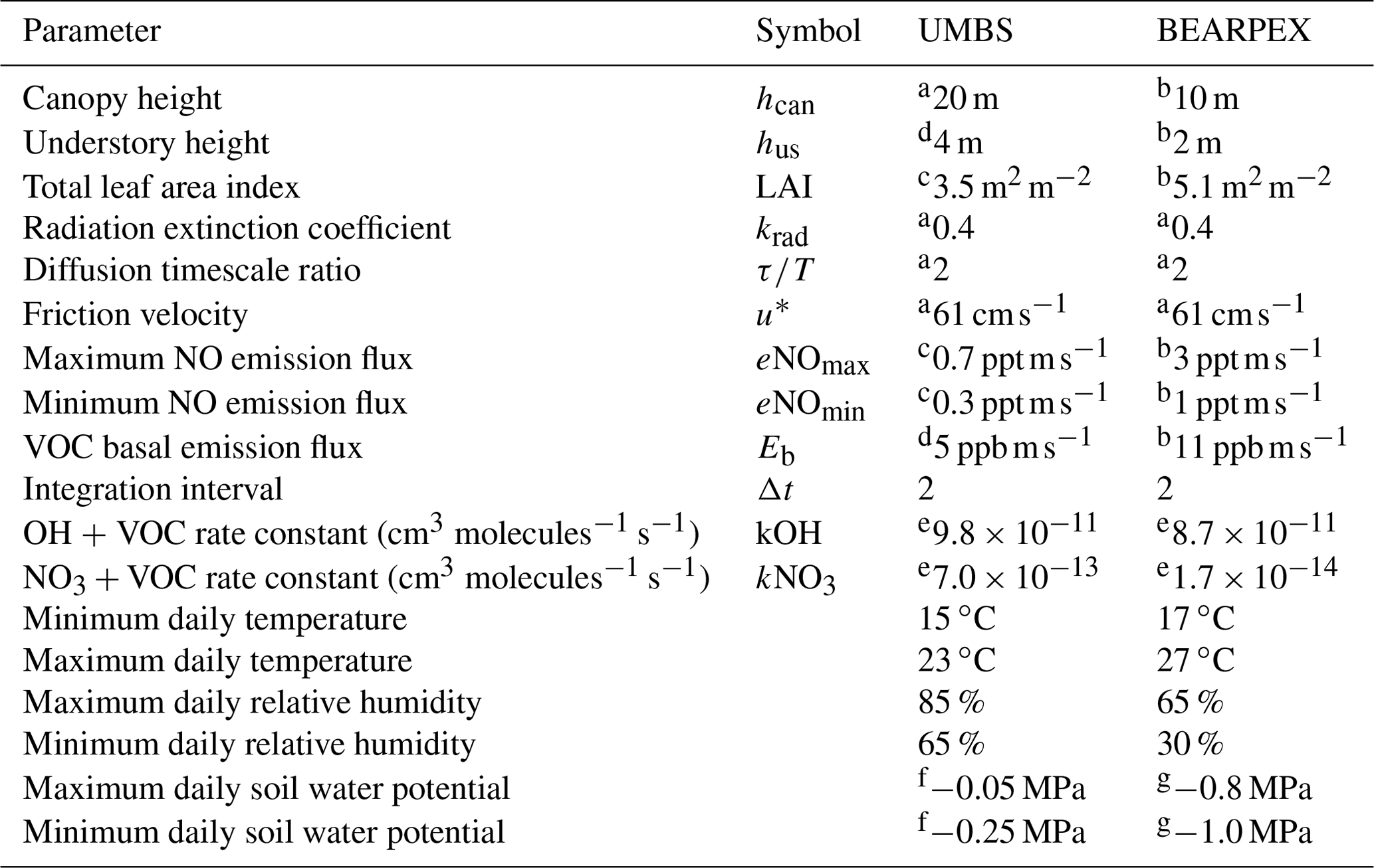
^a Geddes and Murphy (2014). ^b Wolfe and Thornton (2011). ^c Seok et al. (2013). ^d Estimated from Bryan et al. (2015). ^e See text; calculated assuming the dominant volatile organic compound (VOC) is 2-methyl-3-buten-2-ol (MBO) for Blodgett Forest and isoprene for UMBS. ^f Estimated from Matheny et al. (2015). ^g Estimated from Ishikawa and Bledsoe (2000) and Stern et al. (2018).

2.1 Deposition

The deposition flux (F_dep) of each depositing species i in the canopy is calculated according to

$$\begin{array}{}\text{(3)}& F_{\mathrm{dep}}=-V_{\mathrm{d}}\cdot \text{LAI}\cdot C_i,\end{array}$$

where LAI is the leaf area index, and V_d is the deposition velocity. The deposition velocities are calculated according to

$$\begin{array}{}\text{(4)}& V_{\mathrm{d}}={\displaystyle \frac{\mathrm{1}}{R}},\end{array}$$

where R is the total resistance to deposition.

$$\begin{array}{}\text{(5)}& {\displaystyle }& {\displaystyle }{R}_{\text{leaf}}={\left({\displaystyle \frac{\mathrm{1}}{R_{\text{cut}}}}+{\displaystyle \frac{\mathrm{1}}{R_{\mathrm{st}}+R_{\mathrm{m}}}}\right)}^{-\mathrm{1}},\text{(6)}& {\displaystyle }& {\displaystyle }R=R_{\mathrm{a}}+R_{\mathrm{b}}+R_{\text{leaf}},\end{array}$$

where R_a, R_b, R_cut, R_st, and R_m are the aerodynamic, boundary layer, cuticular, stomatal, and mesophilic resistances, respectively. These resistances describe the turbulent transport of a gas to the surface (R_a), molecular transport through a thin layer of air above the leaf surface (R_b), and deposition to the leaf surface (R_leaf) (Baldocchi et al., 1987). R_leaf is dependent upon plant physiology and the chemical and physical properties of the depositing compounds. R_leaf is determined by deposition to the leaf cuticles (R_cut), diffusion through the stomata (R_st), and chemical processing within the mesophyll (R_m). We do not allow for emission of NO or NO₂ from leaves, consistent with recent laboratory observations that have observed negligible compensation points for these molecules (Chaparro-Suarez et al., 2011; Breuninger et al., 2013; Delaria et al., 2018).

All boundary, aerodynamic, cuticular, and soil resistances of O₃, HNO₃, CH₂O, alkyl nitrates (ANs), acyl peroxy nitrates (APNs), HC(O)OH, ROOH, and H₂O₂ are calculated according to Wolfe et al. (2011). The cuticular and mesophyllic resistances for NO₂ and NO are adjustable input parameters. Stomatal resistances are determined from the stomatal conductance to water vapor (g_s) calculated using either Eq. (7) (Wesely, 1989) or Eq. (8) (Jarvis et al., 1976; Emberson et al., 2000), hereafter referred to as the Wesely and Emberson schemes, respectively:

$$\begin{array}{}\text{(7)}& {\displaystyle }{g}_{\mathrm{s}}=g_{\text{max}}\times {\displaystyle \frac{T(\mathrm{40}-T)/\mathrm{400}}{(\mathrm{1}+{\left(\mathrm{200}{\left(\text{SR}+\mathrm{0.1}\right)}^{-\mathrm{1}}\right)}^{\mathrm{2}}}},\text{(8)}& {\displaystyle }\begin{array}{rl}{g}_{\mathrm{s}}& =g_{\text{max}}\\ & \times f_{\text{phen}}\times f_{\text{light}}\times max\left\{f_{\text{min}},(f_{\text{temp}}\times f_{\text{VPD}}\times f_{\text{SWP}})\right\},\end{array}\end{array}$$

where g_max is the species-specific maximum stomatal conductance; f_min is a species-specific scaling factor to the minimum stomatal conductance; SR is the solar radiation in watts per square meter (W m⁻²); and f_phen, f_SWP, f_light, f_temp, and f_VPD are functions representing modifications to the stomatal conductance due to leaf phenology, soil water content, irradiance, temperature, and vapor pressure deficit, respectively (Eqs. 9–12).

$$\begin{array}{}\text{(9)}& {\displaystyle }{f}_{\text{light}}=\mathrm{1}-\exp (-{\text{Light}}_a\times \text{PPFD})\text{(10)}& {\displaystyle }{f}_{\text{temp}}=\mathrm{1}-{\displaystyle \frac{{\left(T-T_{\text{opt}}\right)}^{\mathrm{2}}}{{\left(T_{\text{opt}}-T_{\text{min}}\right)}^{\mathrm{2}}}}\text{(11)}& {\displaystyle }\begin{array}{rl}{f}_{\text{VPD}}& =min\mathit{\{}\mathrm{1},\left(\left(\mathrm{1}-f_{\text{min}}\right)\times {\displaystyle \frac{\left({\text{VPD}}_{\text{min}}-\text{VPD}\right)}{\left({\text{VPD}}_{\text{min}}-{\text{VPD}}_{\text{max}}\right)}}\right)\\ & +f_{\text{min}}\mathit{\}}\end{array}\text{(12)}& {\displaystyle }\begin{array}{rl}{f}_{\text{SWP}}& =min\mathit{\{}\mathrm{1},\left(\left(\mathrm{1}-f_{\text{min}}\right)\times {\displaystyle \frac{\left({\text{SWP}}_{\text{min}}-\text{SWP}\right)}{\left({\text{SWP}}_{\text{min}}-{\text{SWP}}_{\text{max}}\right)}}\right)\\ & +f_{\text{min}}\mathit{\}}\end{array}\end{array}$$

T_opt and T_min are the optimal and minimum temperature required for stomatal opening. PPFD is the photosynthetic photon flux density, and Light_a is a species-specific light response parameter. VPD_min and VPD_max are the vapor pressure deficit at which stomatal opening reaches a minimum and maximum, respectively. SWP_min and SWP_max are the soil water potentials at which stomatal opening reaches a minimum and maximum, respectively. All model calculations represented the peak growing season when f_phen=1. f_temp, f_VPD, and f_light were calculated according to Emberson et al. (2000) using parameters found in Table 2.

Table 2 Parameters used in the Emberson model for stomatal conductance.

2.2 Site description

The model was evaluated with comparison to observations from the Biosphere Effects on Aerosols and Photochemistry 2009 (BEARPEX-2009) field campaign from 15 June to 31 July 2009 at Blodgett Forest (Min et al., 2014) and the University of Michigan Biological Station (UMBS) during 5–10 August 2012 (Geddes and Murphy, 2014). For the BEARPEX-2009 calculations, the modeled canopy included an overstory height of 10 m with a one-sided leaf area index of 3.2 m² m⁻² (LAI_os) and an understory height of 2 m with a LAI of 1.9 m² m⁻² (LAI_us). Model simulations were run for 30 June 2009 using conditions from the BEARPEX-2009 ponderosa pine forest site located in the western foothills of the Sierra Nevada Mountains, CA (38^∘58^′42.9^′′ N, 120^∘57^′57.9^′′ W; elevation 1315 m) (Table 1) (Fig. 2a). Meteorological conditions and soil NO emissions used in the model simulation were those reported by Min et al. (2014). Diurnal soil water potentials (SWPs) were values reported in a geological survey of nearby Sierra sites in a comparatively wet year (Ishikawa and Bledsoe, 2000; Stern et al., 2018).

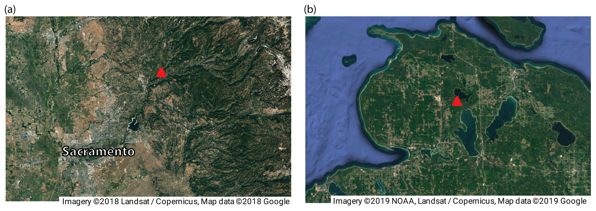
Figure 2 Satellite images showing the locations of (a) the BEARPEX-2009 campaign and (b) the University of Michigan Biological Station (UMBS). Red triangles show the specific site locations. Measurements of chemical species and local meteorological variables from the two campaigns were used to validate our 1-D canopy multibox model.

For UMBS-2012 calculations, the modeled canopy included an overstory height of 20 m with a one-sided LAI of 2.5 m² m⁻² and an understory height of 4 m with a LAI of 1 m² m⁻² (Bryan et al. 2015). Model simulations were run for 8 August 2012 using conditions from the UMBS mixed hardwood forest located in northern Michigan (45^∘33^′32^′′ N, 84^∘42^′52^′′ W) (Table 1) (Fig. 2b). Daily temperatures, VPDs, soil NO emissions, and site-specific parameters used in the model simulations were those reported in Geddes and Murphy (2014) and Seok et al. (2013).

Temperature and relative humidity used in the model were sinusoidal fits to observations of minimum and maximum daily temperature and relative humidity from the corresponding field measurement site. The relative temperature decrease as a function of altitude was calculated using a fit to observations during BEARPEX-2007, as presented by Wolfe and Thornton (2011). Solar zenith angles (SZAs) and photosynthetically active radiation (PAR) were calculated every 0.5 h for each location and time period using the National Center for Atmospheric Research TUV calculator (Madronich and Flocke, 1999) and fit using a smoothed spline interpolation. Within the canopy, extinction of radiation (ER) was calculated following Beer's law:

$$\begin{array}{}\text{(13)}& {\text{ER}}_k=\exp \left(-{\displaystyle \frac{k_{\text{rad}}{\text{LAI}}_{\text{cum}}}{\cos \left(\text{SZA}\right)}}\right),\end{array}$$

where k_rad is the radiation extinction coefficient, SZA is the solar zenith angle, and LAI_cum is the cumulative LAI calculated as the sum of one-half the LAI in box k and the total LAI in the boxes above box k.

2.3 Vertical transport and advection

The turbulent diffusion flux (F(z)) is represented in the model using K-theory, according to the Chemistry of Atmosphere-Forest Exchange (CAFE) Model (Wolfe and Thornton, 2011).

$$\begin{array}{}\text{(14)}& F\left(z\right)=-K\left(z\right){\displaystyle \frac{\mathrm{\Delta }{C}_{i,k}}{\mathrm{\Delta }z}},\end{array}$$

where ΔC_i,k is the change in concentration in species i in box k during each time step, and Δz is the difference between the midpoints of boxes k and k+1. K(z) above the canopy is based on the values from Gao et al. (1993), and below the canopy it is a function of friction velocity calculated according to Wolfe et al. (2011) and is a function of the diffusion timescale ratio (τ∕T_L) – defined as the ratio of the time since emission of a theoretical diffusing plume (τ) and the Lagrangian timescale (T_L) – and the friction velocity (u^∗) (Wolfe and Thornton, 2011). The details of the parameterization of turbulent diffusion fluxes are documented elsewhere (Wolfe and Thornton, 2011) and based on the works of Raupach (1989) and Makar et al. (1999). The height-dependent friction velocity (u(z)^∗) is attenuated from the above-canopy u^∗ according to Yi et al. (2008). Although Finnigan et al. (2015) identified flaws in this treatment, we believe it is sufficient for our focus on illustrating generalizable qualitative trends.

The resulting residence time in the canopy is approximately 2–3 min for model conditions during the day. Our model is a simple parameterization of turbulent processes and as such will only capture mean vertical diffusion. Other works (Collineau and Brunet, 1993a; Raupach et al., 1996; Brunet and Irvine, 2000; Thomas and Foken, 2007; Sörgel et al., 2011; Steiner et al., 2011) have shown that near-field effects of individual canopy elements and coherent turbulent structures can play an important role in canopy exchange. These more intricate processes are not captured explicitly by our simple model. Previous works (Gao et al., 1993; Makar et al., 1999; Stroud et al., 2005; Wolfe et al., 2011) have also utilized fairly simple representations of canopy exchange in local and regional models, and as such K-theory is likely sufficient to represent average vertical diffusion for the purposes of our study.

Advection in the model is treated as a simple mixing process in each model layer.

$$\begin{array}{}\text{(15)}& \left({\displaystyle \frac{\mathrm{d}{C}_i}{\mathrm{d}t}}\right)=-k_{\text{mix}}\left(C_i-C_{i\left(\text{adv}\right)}\right),\end{array}$$

where k_mix=0.3 h⁻¹ (Wolfe and Thornton, 2011), and C_i(adv) is the advection concentration of species i. Advection concentrations are set to fit with the observations during BEARPEX-2009 (Min et al., 2014) or UMBS-2012 (Geddes and Murphy, 2014; Seok et al., 2013) and are used to maintain reasonable background concentrations (Table S1 in the Supplement). Concentrations of NO_x, O₃, and some volatile organic compounds (VOCs) at both sites were influenced by emissions from nearby cities and consequently had sources outside the canopy. For the BEARPEX-2009 model runs, the maximum daily advection concentration was reached at around 17 h, based on field observations of higher NO_x plumes from nearby Sacramento in the afternoon (Wolfe et al., 2011; Min et al., 2014). The diurnal advection concentrations of NO_x were modeled with a sinusoidal function in the range 0.1–0.35 ppb (Table S1). For UMBS all advection concentrations were constant.

2.4 Chemistry

Chemistry in the model is based on reaction rate constants from the JPL Chemical Kinetics and Photochemical Data for Use in Atmospheric Studies evaluation no. 18 (Burkholder et al., 2015). Photolysis rates are calculated as a function of solar zenith angle (SZA), which was constructed using a smoothed spline interpolation fit of photolysis rates calculated with the TUV calculator (Madronich and Flocke, 1999) at every 10^∘ interval of the zenith angle. The simplified reaction scheme included in the model is based on the model presented in Browne and Cohen (2012). The model includes both daytime and nighttime NO_x chemistry and a simplified oxidation scheme. In this simplified case, oxidation of VOCs during the daytime results in the production of peroxy radicals (RO₂), treated as a uniform chemical family. To be applicable to a range of forest types, we also include adjustable parameters, kOH and kNO₃ for the average rate constant for reaction of VOCs with OH and NO₃, respectively. kOH and kNO₃ are effective values adjusted in the model based on site-specific VOC composition and observations of OH reactivity. A complete list of reactions and rate constants included in the model is shown in Table S2.

2.5 BVOC emissions

Emissions rates (molecules ${\mathrm{cm}}^{-\mathrm{3}}{\mathrm{s}}^{-\mathrm{1}}$) of biogenic volatile organic compounds (BVOCs) in the canopy are calculated via

$$\begin{array}{}\text{(16)}& E\left(z\right)={\displaystyle \frac{E_{\mathrm{b}}}{\mathrm{\Delta }h}}{C}_{\mathrm{L}}\left(z\right)C_{\mathrm{T}}\left(z\right)\text{LAI},\end{array}$$

where E_b (molecules cm(leaf)⁻² s⁻¹) is the basal emission rate of VOC, Δh is the total height of the box, and C_L and C_T are corrections for light and temperature (Guenther et al., 1995).

2.6 Evaluation of NO_x fluxes and lifetimes

The model was used to assess the impact of NO₂ deposition parameters on the NO_x budget, lifetime, loss, and vertical profile within a forested environment. In each box, the rates of NO_x loss with respect to nitric acid formation, alkyl nitrate formation, and deposition were calculated from Eqs. (17)–(19).

$$\begin{array}{}\text{(17)}& {\displaystyle }\begin{array}{rl}& L_{{\mathrm{NO}}_x\to {\mathrm{HNO}}_{\mathrm{3}}}=k_{\mathrm{OH}+{\mathrm{NO}}_{\mathrm{2}}}\left[\mathrm{OH}\right]\left[{\mathrm{NO}}_{\mathrm{2}}\right]+k_{{\mathrm{N}}_{\mathrm{2}}{\mathrm{O}}_{\mathrm{5}}\text{hydrolysis}}\left[{\mathrm{N}}_{\mathrm{2}}{\mathrm{O}}_{\mathrm{5}}\right]\\ & +k_{{\mathrm{NO}}_{\mathrm{3}}+\text{aldehyde}}\left[\text{aldehyde}\right]\left[{\mathrm{NO}}_{\mathrm{3}}\right]\end{array}\text{(18)}& {\displaystyle }\begin{array}{rl}& L_{{\mathrm{NO}}_x\to {\mathrm{RONO}}_{\mathrm{2}}}=\mathit{\alpha }{k}_{\mathrm{NO}+{\mathrm{RO}}_{\mathrm{2}}}\left[\mathrm{NO}\right]\left[{\mathrm{RO}}_{\mathrm{2}}\right]\\ & +\mathit{\beta }{k}_{{\mathrm{NO}}_{\mathrm{3}}}\left[{\mathrm{NO}}_{\mathrm{3}}\right]\left[\text{BVOC}\right]\end{array}\text{(19)}& {\displaystyle }{L}_{{\mathrm{NO}}_x\to \text{Dep}}=F_{\text{dep}}/\mathrm{\Delta }{h}_k\end{array}$$

α is the fraction of the NO+RO₂ reaction that forms alkyl nitrates, and β is the fraction of the NO₃+BVOC reaction that forms alkyl nitrates. The NO_x lifetime was then scaled to the entire boundary layer by summing over the products of the lifetime and boundary layer fraction (Δh_k∕PBL) in each box.

$$\begin{array}{}\text{(20)}& {\mathit{\tau }}_{\text{PBL}}={\displaystyle \frac{{\sum }_{k=\mathrm{1}}^{\mathrm{8}}{\left[{\mathrm{NO}}_x\right]}_k}{{\sum }_{k=\mathrm{1}}^{\mathrm{8}}\left(L_{{\mathrm{NO}}_x\to \text{Dep}}+L_{{\mathrm{NO}}_x\to {\mathrm{RONO}}_{\mathrm{2}}}+L_{{\mathrm{NO}}_x\to {\mathrm{HNO}}_{\mathrm{3}}}\right)}}\end{array}$$

NO_x was treated as the sum of NO, NO₂, and all short-lived products, including NO₃, 2N₂O₅, and peroxyacetyl nitrate (PAN) (Romer et al., 2016). Deposition of PAN was not considered.

We also calculated the 24 h average vertical fluxes (Eq. 14) of NO_x and used the flux through the canopy to estimate the fraction of soil-emitted NO_x ventilated to the troposphere above. Because PAN formed during the nighttime is expected to rerelease NO_x to the atmosphere during the day, in this calculation, PAN was included as part of the NO_x budget.

3 Sensitivity to parameterizations

We assessed the sensitivity of the model to τ∕T_L, the radiation extinction coefficient (k_rad), the aerodynamic leaf width (l_w), LAI, soil NO emission (eNO), and α. These parameters are simplifications of complex physical processes and not always easily constrained by observations. The total deposition velocity of NO₂ chosen for these assessments was 0.2 cm s⁻¹ during the daytime and 0.02 cm s⁻¹ during the nighttime, based on values of g_max and g_min chosen for Blodgett Forest (discussed above) and typical values for deposition velocity observed for a variety of species in the laboratory (Teklemariam and Sparks, 2006; Chaparro Suarez et al., 2011; Breuninger et al., 2013; Delaria et al., 2018).

The largest effects were observed for changes in α, LAI, and soil NO emission. LAI_os and LAI_us were scaled from their values of 1.9 and 3.2 m² m⁻², respectively, by a factor of 0.25 and 1.5. Increasing the scaling factor from 0.25 to 1.5 resulted in a decrease in NO_x lifetimes, above-canopy concentration, and average canopy flux of 24 %, 27 %, and 36 %, respectively (Fig. S1 in the Supplement). Increasing α from 0.01 to 0.1 resulted in a decrease in NO_x lifetimes, above-canopy concentrations, and average canopy fluxes of 75 %, 38 %, and 39 %, respectively (Fig. S2). For all other model runs an α of 0.075 was chosen, in accordance with observations from regions primarily influenced by BVOCs (e.g., monoterpenes, isoprene, 2-methyl-3-buten-2-ol). Increasing the maximum soil NO emission from 1 to 10 ppt m s⁻¹ increased the in-canopy enhancement from 28 % to 140 % relative to above-canopy NO_x concentrations (Fig. S3b). The fraction of soil-emitted NO_x ventilated through the canopy also increased from 45 % to 64 % (Fig. S3a). The large effect of soil NO emission on NO_x fluxes implies that this highly variable parameter (Vinken et al., 2014) is also important to constrain in chemical transport models. Further discussion of soil NO emission is, however, beyond the scope of this study.

Very small effects on NO_x were observed for changes in the parameters τ∕T_L, k_rad, or l_w. The minor changes caused by variations in these parameters are listed below for completeness.

τ∕T_L represents the diffusion timescale ratio, a full description of which can be found in Wolfe and Thornton (2011). A larger τ∕T_L represents faster diffusion and vertical transport within the canopy layer, as well as shorter residence times in the canopy. We find that altering this parameter from 1.2 to 8 (representing a change in residence time from 650 to 62 s) caused a 9.9 %, 4.4 %, and 8.7 % increase in average canopy fluxes, NO_x lifetimes, and above-canopy concentration, respectively (Fig. S4). For all subsequent model runs, a value of 2 for τ∕T_L was chosen, resulting in a canopy residence time during the day of 152 and 194 s for Blodgett Forest and UMBS, respectively, calculated using Eq. (21).

$$\begin{array}{}\text{(21)}& {\mathit{\tau }}_{\text{can}}=h_{\text{can}}\sum _{k=\mathrm{1}}^{\mathrm{3}}{\displaystyle \frac{\mathrm{\Delta }{h}_k}{K\left(z_k\right)}}\end{array}$$

The boundary layer resistance, or laminar sublayer resistance, R_b, is dependent upon the aerodynamic leaf width, l_w (Eq. 22):

$$\begin{array}{}\text{(22)}& R_{\mathrm{b}}={\displaystyle \frac{c\mathit{\nu }}{D{u}^{\ast }\left(z\right)}}{\left({\displaystyle \frac{l_{\mathrm{w}}{u}^{\ast }\left(z\right)}{\mathit{\nu }}}\right)}^{\mathrm{1}/\mathrm{2}},\end{array}$$

where ν=0.146 cm² s⁻¹ is the kinematic viscosity of air, D is the species-dependent molecular diffusion coefficient, c is a tunable constant set to 1 for this study, and u^∗(z) is the height-dependent friction velocity that is a function of u^∗ and LAI_cum (Wolfe and Thornton, 2011). l_w depends upon the vegetation species. A value of 1 cm was chosen for the overstory and 2 cm for the understory, as these widths are characteristic of pine trees and understory shrubs in a ponderosa pine forest (Wolfe and Thornton, 2011). Species with rapid deposition to the cuticles or the stomata are expected to be more sensitive to errors in l_w, such as HNO₃ or H₂O₂. An increase in NO_x lifetime, average canopy flux, and above-canopy concentration of 1.4 %, 2.4 %, and 2.8 %, respectively, was predicted for a change in l_w scaling factor from 0.1 to 2 (Fig. S5). These changes are expected to be greater in forests with a larger average deposition velocity, where R_b makes a greater contribution to the total resistance.

The rates of stomatal gas exchange and photolysis are regulated by the intensity of light that penetrates the canopy. The extinction of radiation by the canopy, treated as a Beer law parameterization (Eq. 13), is exponentially proportional to the radiation extinction coefficient, k_rad. k_rad ranging from 0.4–0.65 has been measured for coniferous forests and understory shrubs (Wolfe and Thornton, 2011). The NO_x lifetime increased by 2.7 %, and the canopy fluxes and above-canopy concentrations decreased by 0.7 % and 0.6 %, respectively, for a change in k_rad from 0 to 0.6 (Fig. S6). This effect is expected to be greater for forests with a larger LAI. The minimal effect of k_rad on model results was also observed for multiple canopy profile shapes of equivalent LAI.

4 Results

4.1 Model validation: comparison to field observations

To evaluate the applicability of our 1-D multilayer canopy model for predicting NO_x concentrations and vertical fluxes in a variety of forest environments, we compared the model to observations from BEARPEX-2009 and UMBS-2012. Parameters used in each calculation are shown in Table 1. The model was run using both the Emberson and Wesely stomatal conductance models. Parameters for temperature, drought stress, and maximum and minimum stomatal conductances used in the Emberson model were input for the dominant tree species in the region (Table 2). At the BEARPEX-2009 site, the dominant tree species was ponderosa pine. For this site, g_max and parameters for f_SWP and f_VPD were inferred from ponderosa pine stomatal conductance data (Kelliher et al., 1995; Ryan et al., 2000; Hubbard et al., 2001; Johnson et al., 2009; Anderegg et al., 2017), and f_light was inferred from measurements of the canopy conductance during BEARPEX-2009 (Fig. 3a). f_temp was represented by observations for Scots pine (Altimir et al., 2004; Emberson et al., 1997; Buker et al., 2012) and validated with comparison to stomatal conductance measured via sap flow during BEARPEX-2009 (Fig. 3a). At UMBS the dominant species are quaking aspen and bigtooth aspen, with many birch, beech, and maple species also present (Seok et al., 2013). Data for a European beech tree species were used to represent stomatal conductance parameters (Buker et al., 2007; Buker et al., 2012) and SWP stress (Emberson et al., 2000). These parameters were validated with comparison to stomatal conductance calculated from water vapor and latent heat flux measurements during UMBS-2012 using an energy-balance method according to Mallick et al. (2013) (Fig. 4a).

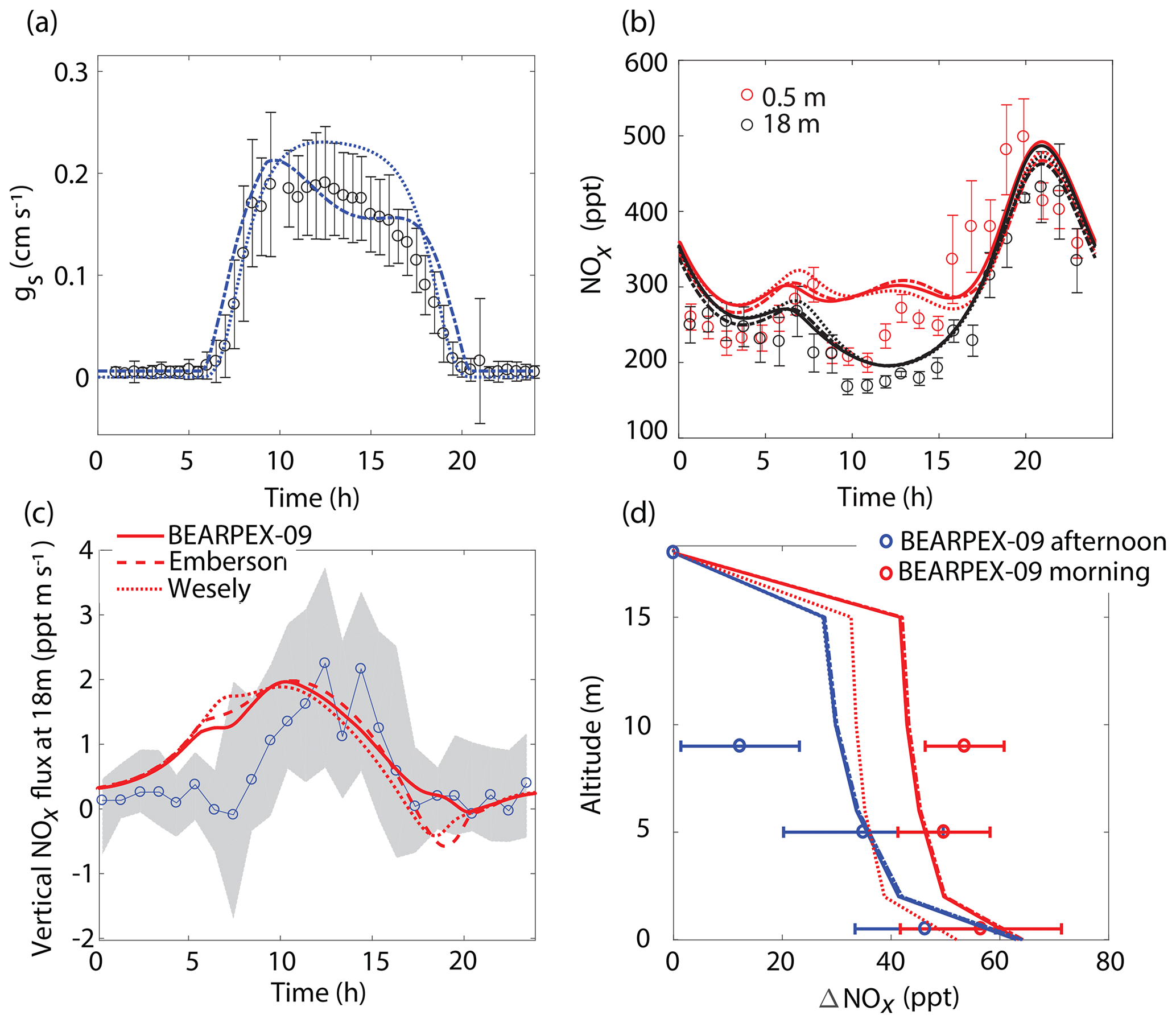
Figure 3 Comparison of model results to BEARPEX-2009 hourly averaged observations of (a) stomatal conductances, (b) NO_x mixing ratios at 18 m (black) and 0.5 m (red), and (c) vertical fluxes at 18 m. (d) Averaged observations of in-canopy NO_x enhancements from 09:00 to 12:00 (blue) and from 13:00 to 16:00 (red) compared with modeled NO_x enhancements, defined as the difference between NO_x below the canopy and NO_x measured at 18 m. Observations from BEARPEX-2009 are from Min et al. (2014). In all panels solid lines, dotted lines, and dashed lines represent results from our model with stomatal conductances parameterized using observed conductances, the Wesely model, and the Emberson model, respectively. Circles, error bars, and grey shaded regions represent observations, standard errors of the mean, and the interquartile range of data, respectively.

The model replicates key features of the canopy fluxes and above-canopy NO_x daytime mixing ratios from the 2009 BEARPEX campaign (Fig. 3). The average daytime above-canopy NO_x mixing ratios during the duration of BEARPEX-2009 was 253 ppt, with observations ranging from 80 to 550 ppt of NO₂ and from 10 to 100 ppt of NO (Min et al., 2014). The general daily trends in observations of NO_x mixing ratios are captured by both the Wesely and Emberson cases – with minimum NO_x mixing ratios occurring in the late morning, an increase in NO_x in the afternoon, and maximum NO_x concentrations of 450–500 ppt reached in the evenings, primarily as a result of high-NO_x plumes from nearby Sacramento in the afternoon (Wolfe et al., 2011; Min et al., 2014) (Fig. 3b). However, both model scenarios predict a slower-than-observed decrease in NO_x mixing ratios from the evening to the early morning, predict larger midmorning fluxes than observed (by ∼0.5–1.5 ppt m s⁻¹), and fail to represent the in-canopy enhancement of NO_x (∼50 ppt), relative to above-canopy mixing ratios, observed in the evening (Fig. 3). The above-canopy vertical NO_x flux predicted in both model cases also agrees reasonably well with observations, with the Emberson case representing morning and midday NO_x fluxes slightly better than the Wesely case. This relatively good agreement between the Emberson case and observed fluxes is also demonstrated in Fig. 3d by the agreement between modeled and observed canopy NO_x enhancements. There is, however, generally little difference between Emberson and Wesely model cases for this site during the period considered (Fig. 3). This is likely due to the good agreement in both the Emberson and Wesely cases with observations of stomatal conductance (Fig. 3a).

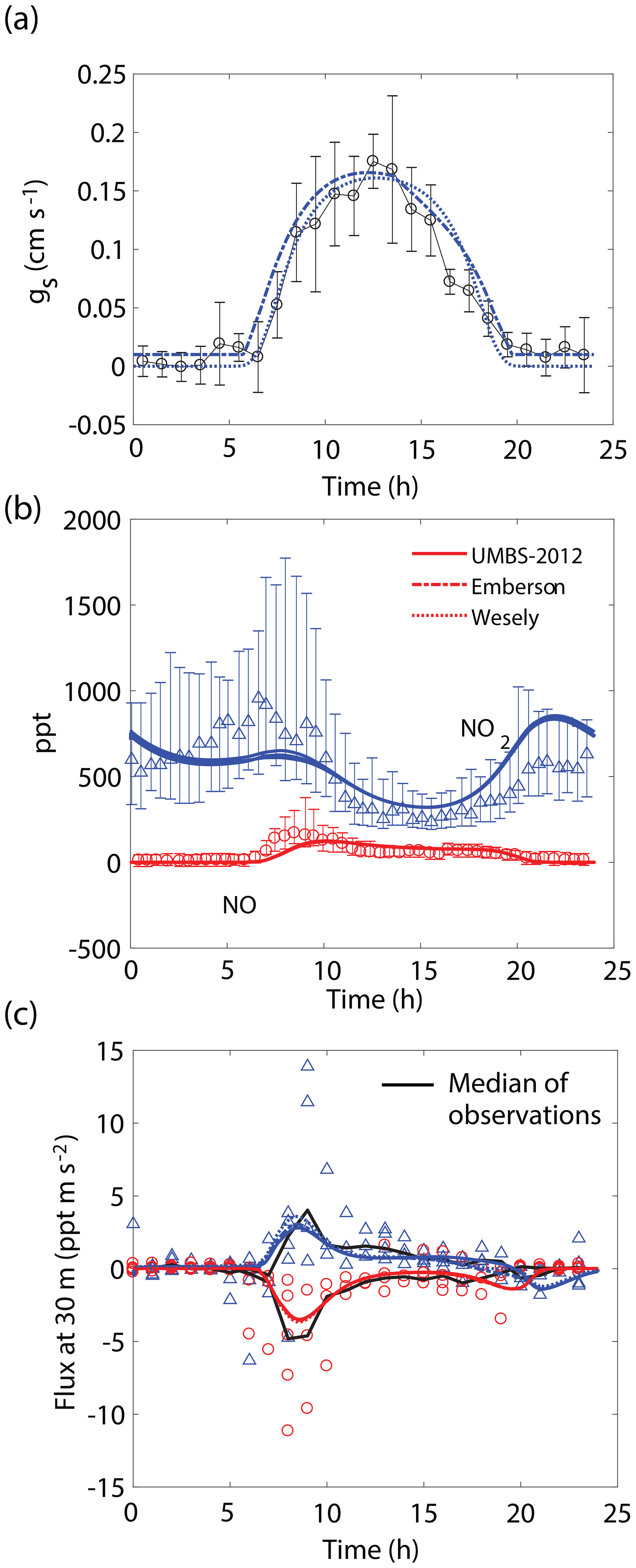
Figure 4 Comparison of model results to (a) hourly averaged observed stomatal conductances, (b) NO and NO₂ mixing ratios at 30 m, and (c) median (black lines) and hourly averaged NO and NO₂ vertical fluxes at 30 m observed during UMBS-2012 for 8 August 2012. In all panels solid lines, dotted lines, and dashed lines represent results from our model with stomatal conductances parameterized using observed conductances, the Wesely model, and the Emberson model, respectively. Blue triangles and red circles represent NO₂ and NO observations, respectively. Error bars represent the interquartile range of data.

We also observe similar correspondence between the model and key features of the UMBS-2012 observations (Fig. 4). NO and NO₂ mixing ratios and canopy fluxes are both within the range of observations. The model predicts a maximum of ∼40 % lower NO₂ in the morning and ∼30 % higher NO₂ at night than what was observed (Fig. 4b). It should also be noted that this agreement was achieved without inclusion of an NO₂ compensation point, whereas Seok et al. (2013) had proposed the importance of considering foliar NO₂ emission at this location. Differences between the Wesely model and Emberson model were negligible for this site. This is likely due to a higher humidity in the summer in this region and larger soil moisture, reducing the prediction for midday and late afternoon VPD stress by the Emberson model, as can be seen by the similarity in the predicted g_s by the Emberson and Wesely models (Fig. 4a).

4.2 Effects of maximum stomatal conductance

The BEARPEX-2009 case was simulated using the Wesely model for different values of the maximum stomatal conductance (g_max) (Fig. 5), with advection concentrations of NO_x set to zero. The range of g_max currently represented in the literature during the peak growing season for forested regions ranges from 0.2 to 0.8 cm s⁻¹ (Kelliher et al., 1995; Emberson et al., 1997; Emberson et al., 2000; Ryan et al., 2000; Hubbard et al., 2001; Altimir et al., 2003; Fares et al., 2013). This range reflects differences in forest types and a wide variety of tree species. Global chemical transport models (CTMs) using the Wesely parameterization currently include g_max of 1.4, 0.77, and 1 cm s⁻¹ for deciduous, coniferous, and mixed forests, respectively (Wesely, 1989; Wang et al., 1998a). Figure 5b demonstrates the impact of g_max on the average daily vertical flux of NO_x through the canopy. A total of 96 % of soil-emitted NO_x is ventilated through the canopy with no foliar deposition (g_max=0 cm s⁻¹). In contrast, 44 % of soil-emitted NO_x is taken up by the forest and 56 % is ventilated through the canopy when the maximum stomatal conductance is 1.4 cm s⁻¹. Figure 5c and d show the effects of g_max on the diurnal flux through the canopy and the diurnal above-canopy NO_x mixing ratio, respectively. Compared with no foliar deposition, a g_max of 1.4 cm s⁻¹ results in ∼60 % reduction in the canopy flux and ∼50 % reduction in the above-canopy NO_x mixing ratio at noon. (Fig. 5c and d). In Fig. 6a we show the fraction of soil-emitted NO_x ventilated through the canopy as a function of g_max. The model suggests a maximum foliar reduction of NO_x of ∼60 % for a canopy of 10 m and total LAI of 5.1 m² m⁻². Our model also predicts that changes in g_max have a greater overall impact on canopy NO_x fluxes at larger leaf resistances and slower foliar uptake. In the range for g_max of ∼0–0.5 cm s⁻¹, variation in g_max can have a large impact on the predicted canopy fluxes of NO_x, which would in turn have a large impact on concentrations and fluxes of O₃. These values of g_max result in deposition velocities in the range expected for most forests, based on laboratory measurements of leaf-level deposition (Hanson and Lindberg, 1991; Rondon and Granat, 1994; Hereid and Monson, 2001; Teklemariam and Sparks, 2006; Pape et al., 2009; Chaparro-Suarez et al., 2011; Breuninger et al., 2013; Delaria et al., 2018) and global analysis suggesting 20–50 % reductions in soil-emitted NO_x by vegetation (Jacob and Wofsy, 1990; Yienger and Levy, 1995; Ganzeveld et al., 2002a, b). Model calculations also predict a strong effect on the lifetimes of NO_x, as shown in Fig. 6b, with maximum stomatal conductances of 0.1, 0.3, and 1.4 cm s⁻¹ reducing the NO_x lifetime by ∼0.7 h (∼7 %), ∼1.8 h (∼18 %), and ∼3.6 h (∼36 %), respectively, compared with no deposition. Similar trends (not shown) were also observed using parameters for UMBS.

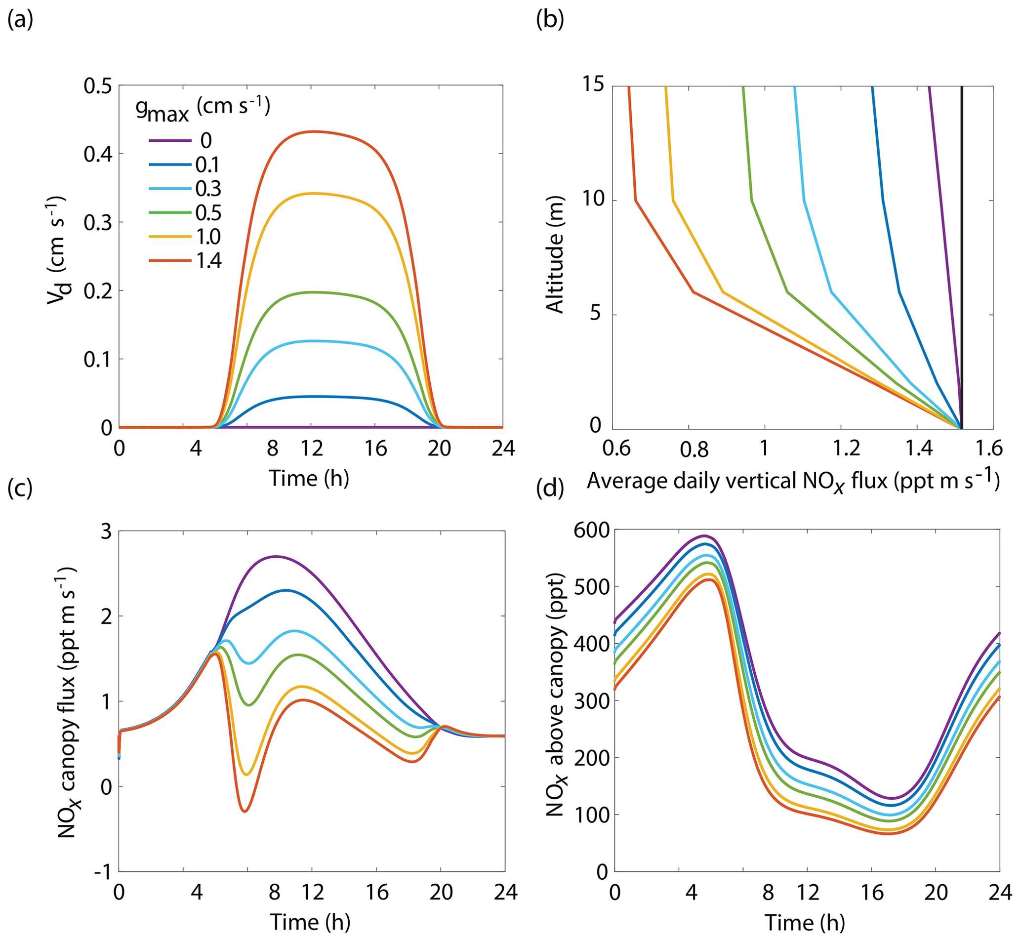
Figure 5 Model results of (a) diurnal NO₂ deposition velocities, (b) average daily vertical fluxes of NO_x and a conserved tracer (black line), (c) diurnal canopy fluxes at 10 m, and (d) diurnal above-canopy NO_x mixing ratios at 15 m for different values of maximum stomatal conductance (g_max) using the Wesely scheme to calculate stomatal conductance.

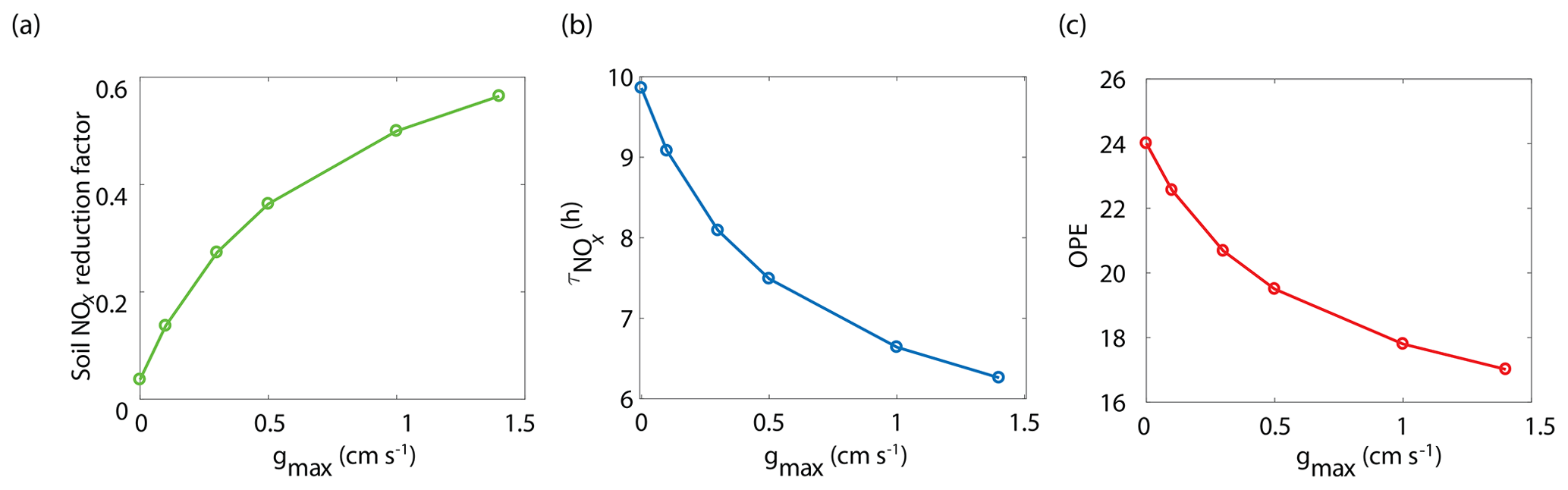
Figure 6 Model-predicted dependence of (a) the fraction of soil-emitted NO_x removed in the canopy, (b) the average daily NO_x lifetime (${\mathit{\tau }}_{{\mathrm{NO}}_x}$) in the planetary boundary layer, and (c) ozone production efficiency (OPE) on maximum stomatal conductance (g_max) using the Wesely scheme to calculate stomatal conductance.

4.3 Emberson model vs. Wesely model comparison

The relative importance of including parameterizations of VPD and SWP in the calculation of stomatal conductance and overall deposition velocity is expected to be regionally variable, along with regional variations in dominant tree species, soil types, and meteorology. We ran the model using BEARPEX-2009 conditions using both the Wesely and Emberson stomatal conductance models under “dry” and “wet” conditions. Here we use “dry” to refer to conditions of low humidity and low soil moisture and “wet” to refer to conditions with high humidity and high soil moisture. Under the dry scenario the SWP daily minimum and maximum were −2.0 and −1.7 MPa, respectively, with the daily minimum reached at sunset. A minimum daily RH of 40 % occurred at noon, with a maximum at midnight of 65 %. Summertime is often even drier in regions of the western United States, so these dry parameters are conservative estimates for many forests. Under the wet scenario the SWP daily minimum and maximum were −0.5 and −0.1 MPa, respectively. The maximum and minimum RH were 90 % and 80 %, respectively. The values for soil moisture and relative humidity chosen were based on observations of SWP by Ishikawa and Bledsoe (2000) and the long-term climate data record at Auburn Municipal Airport (38.9547^∘ N, −121.0819^∘ W) from the NOAA National Centers for Environmental Information.

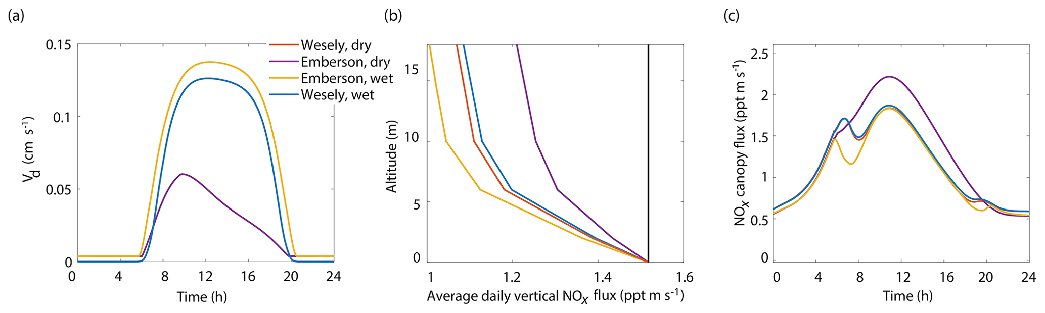
Figure 7 Modeled results of (a) diurnal NO₂ deposition velocities, (b) average daily vertical fluxes compared to a conserved tracer (black line), and (c) diurnal canopy fluxes at 10 m for wet and dry scenarios using either the Wesely or Emberson models to calculate stomatal conductance.

The results of the Wesely and Emberson wet and dry model runs are shown in Fig. 8. There was only a slight decrease in the in-canopy NO_x enhancement and the canopy flux in the Wesely wet case, presumably due to a slight increase in OH radicals at higher RH. Predictably, the difference in the modeled deposition velocities was quite dramatic between the Emberson wet and dry cases. In the dry scenario, the deposition velocity reached a maximum in the late morning but rapidly declined after noon. The maximum deposition velocity reached was also substantially reduced (Fig. 7a). Using the wet Emberson stomatal conductance model, the NO_x flux out of the forest was reduced by 16 % midday compared to the dry case, and the percent of soil NO_x removed within the canopy was increased from 18 % to 30 % (Fig. 7). The model calculates a substantial impact on above-canopy NO_x mixing ratios (Fig. 8), with a maximum of ∼30 % difference in NO_x in the afternoon between wet and dry days using the Emberson parameterization, compared with ∼10 % difference using the Wesely model. Using the Emberson parameterization of stomatal conductance, deposition during wet days is predicted to contribute substantially more to the total NO_x loss (∼40 %), with only ∼15 % contribution predicted for dry days (Fig. 9).

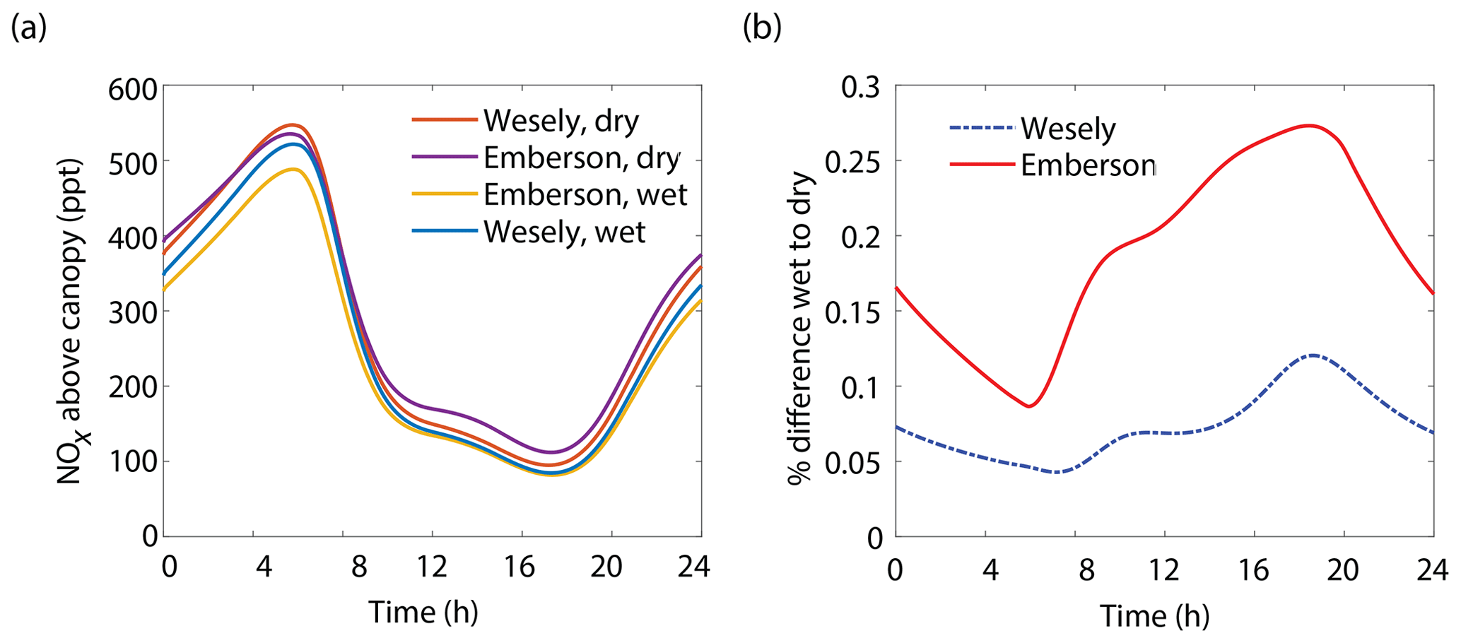
Figure 8 (a) Modeled NO_x mixing ratios above the canopy at 18 m for wet and dry scenarios using either the Wesely or Emberson models to calculate stomatal conductance. (b) Percent difference between NO_x mixing ratios on wet and dry days using either the Wesely (dashed blue line) or Emberson (solid red line) parameterization of stomatal conductance.

Under the Wesely model, where stomatal conductance is parameterized only with temperature and solar radiation, the predicted deposition velocity would be nearly identical between the spring and fall in the western United States and similar semiarid regions (with comparatively minor temperature effects). While the Emberson model predicts large seasonal differences, the Wesely model fails to account for the dramatic decrease in stomatal conductance seen in the dry seasons in such regions caused by significant reductions in relative humidity and soil water potential (Prior et al., 1997; Panek and Goldstein, 2001; Chaves, 2002; Beedlow et al., 2013). We recognize that the multibox model presented in this work is a simplified representation of physical processes and as such is not likely to (and is not intended to) provide quantitative exactitude for the trends described above. However, we argue for the necessity of incorporating these conceptual advances for accurately representing canopy processes and predicting their effect on the NO_x cycle.

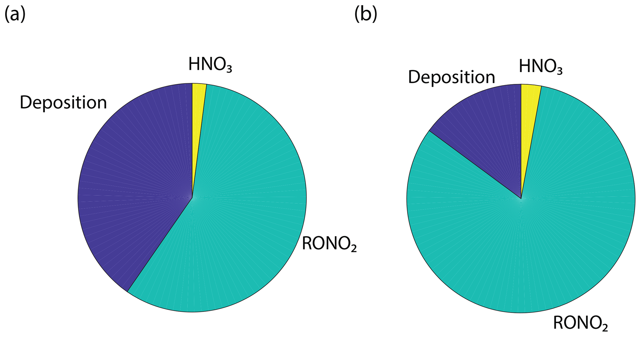
Figure 9 Model prediction for the daytime average fraction of NO_x removed by deposition, nitric acid formation, and alkyl nitrate formation using the Emberson parameterization of stomatal conductance for (a) wet and (b) dry conditions.

5 Discussion

5.1 Implications for modeling NO₂ dry deposition

As in our multilayer canopy model, the most common current method of parameterizing stomatal and cuticular deposition in large-scale chemical transport models (CTMs) is through the resistance model framework of Baldocchi et al. (1987). Many global (e.g., WRF-Chem and GEOS-Chem) and regional (e.g., MOZART and CAMx) CTMs calculate the stomatal component of the total deposition resistance using the representation of Wesely (1989), where stomatal conductance is dependent only on the type of vegetation, temperature, and solar radiation. The limitations of this parameterization have been highlighted by observations of a strong dependence of foliar deposition on soil moisture and vapor pressure deficit (VPD) (Kavassalis and Murphy, 2017; Rydsaa et al., 2016). Inadequate descriptions of vegetative species, soil moisture, drought stress, etc., can have a dramatic impact on model results and can result in significant discrepancies between models and observations (Wesely and Hicks, 2000). Failure to account for effects of plant physiology on deposition may result in misrepresentation of deposition velocities, which, as we demonstrate, can have a substantial impact on NO_x lifetimes and mixing ratios above and within a forest canopy. This effect will be especially pronounced in areas such as much of the western United States, where there are frequent periods of prolonged drought. Parameterizations of stomatal conductance, such as those presented in Emberson et al. (2000) and incorporated into some regional-scale CTMs (e.g., EMEP, MSC-W, and CHIMERE), if incorporated into global atmospheric models, could more accurately reflect the dependence of foliar deposition on meteorology and soil conditions. However, additional laboratory and field measurements on diverse plant species are also needed to determine appropriate, ecosystem-specific inputs to these parameterizations.

It should be noted that there have been significant recent advances in optimization approaches of stomatal modeling based on the theory that stomata maximize CO₂ assimilation per molecule of water vapor lost via transpiration (Medlyn et al., 2011; Bonan et al., 2014; Franks et al., 2017; Miner et al., 2017; Franks et al., 2018). Medlyn et al. (2011) reconciled the empirical widely utilized Ball–Berry model with a theoretical framework optimizing ribulose-1,5-bisphosphate (RuBP) regeneration-limited photosynthesis. However, such methods of water use efficiency optimization do not account for stomatal closure as a result of soil moisture stress. Bonan et al. (2014) further developed a model considering water use efficiency optimization and water transport between the soil, plant, and atmosphere. Such parameterizations are utilized in the Community Land Model (CLM) – a land surface model often incorporated into regional and global climate–chemistry models (Lombardozzi et al., 2015; Kennedy et al., 2019). Although this model provides a physiological and mechanistic basis for stomatal behavior, it is heavily parameterized, relying on inputs of plant and soil parameters that could be expected to vary significantly across ecosystem types. For this reason, we view these methods as aspirational for incorporation into atmospheric global CTMs. We find the relative simplicity of the Emberson approach more useful for the purpose and scope of parameters for large-scale atmospheric models.

5.2 Implications for modeling ozone

NO₂, as well as O₃, deposition budgets are frequently calculated through inferential methods whereby the deposition velocity is constrained with ambient observations (Holland et al., 2005; Geddes and Murphy, 2014). These inferential models are often complicated by the fast reaction of the NO₂–NO–O₃ triad, making it difficult to separate chemical and physical processes. Further, these inferential models for determining dry deposition constrained with observations of chemical concentrations and eddy-covariance measurements of fluxes are difficult to interpret because of similar chemical and turbulent timescales (Min et al., 2014; Geddes and Murphy, 2014). Emission of NO from soils, rapid chemical conversion to NO₂, and subsequent in-air reactions of NO_x must be evaluated accurately in order to correctly infer NO_x and O₃ atmosphere–biosphere exchange from observations. Our multilayer canopy model applies a simple method of representing these processes and evaluating the separate effects of chemistry and dry deposition on the NO_x budget in forests.

Since the foliar deposition of NO₂ reduces the NO_x lifetime and NO_x that is transported out of the canopy, it will also reduce the amount of ozone that is produced both within and above the canopy. Ozone production efficiency (OPE) in the canopy is calculated using Eqs. (23)–(25):

$$\begin{array}{}\text{(23)}& {\displaystyle }L\left({\mathrm{NO}}_{\mathit{\text{x}}}\right)=L_{{\mathrm{NO}}_x\to \text{Dep}}+L_{{\mathrm{NO}}_x\to {\mathrm{RONO}}_{\mathrm{2}}}+L_{{\mathrm{NO}}_x\to {\mathrm{HNO}}_{\mathrm{3}}},\text{(24)}& {\displaystyle }\begin{array}{rl}& P\left({\mathrm{O}}_{\mathrm{3}}\right)=k_{{\mathrm{HO}}_{\mathrm{2}}+\mathrm{NO}}\left[{\mathrm{HO}}_{\mathrm{2}}\right]\left[\mathrm{NO}\right]+k_{{\mathrm{CH}}_{\mathrm{3}}{\mathrm{O}}_{\mathrm{2}}+\mathrm{NO}}\\ & \left[{\mathrm{CH}}_{\mathrm{3}}{\mathrm{O}}_{\mathrm{2}}\right]\left[\mathrm{NO}\right]+\left(\mathrm{1}-\mathit{\alpha }\right)k_{{\mathrm{RO}}_{\mathrm{2}}+\mathrm{NO}}\left[{\mathrm{RO}}_{\mathrm{2}}\right]\left[\mathrm{NO}\right],\end{array}\text{(25)}& {\displaystyle }\text{OPE}={\displaystyle \frac{P\left({\mathrm{O}}_{\mathrm{3}}\right)}{L\left({\mathrm{NO}}_{\mathit{\text{x}}}\right)}},\end{array}$$

where P(O₃) is the ozone production rate and L(NO_x) is the NO_x loss rate. The effect of stomatal conductance to NO₂ on OPE is shown in Fig. 6c. An increase in g_max from 0 to 0.3 cm s⁻¹ results in a decrease in OPE for the PBL from 24.0 to 20.7 (∼14 %) and a decrease to 17.0 (∼30 %) if g_max is 1.4 cm s⁻¹. This is similar to OPE calculations that have been reported for forests and environments with NO_x mixing ratios less than 1 ppb and heavily influenced by BVOC emissions (Marion et al., 2001; Browne and Cohen, 2012; Ninneman et al., 2017).

NO₂ deposition and the in-canopy chemistry of NO₂–NO–O₃ also impact O₃ production and removal. O₃ deposition is frequently inferred from measurements of O₃ concentrations or eddy-covariance measurements (Wesely and Hicks, 2000; Kavassalis and Murphy, 2017). However, because NO₂ has a direct impact on ozone production, deposition of NO₂ can affect inferences of O₃ deposition from observations. The 14 % reduction of OPE and the more-than-20 % reduction in daytime NO_x resulting from an increase in g_max from 0 to 0.3 cm s⁻¹ can cause a parallel decrease in O₃ concentrations and fluxes independent of O₃ chemical loss or deposition. Thus, deposition of NO₂ must be taken into account when evaluating O₃ deposition losses from observed canopy fluxes.

5.3 Implications for near-urban forests

The analysis above suggests that the relative importance of chemical sinks and deposition will vary with NO_x concentration. To evaluate the relative importance of NO₂ foliar deposition and chemistry as a function of NO_x mixing ratio, a simplified single-box model was also constructed with a simplified reaction scheme (Table S3), VOC reactivity of 8 s⁻¹, α of 0.075, and a HO_x (${\mathrm{HO}}_{\mathrm{x}}\equiv \mathrm{OH}+{\mathrm{HO}}_{\mathrm{2}}$) production rate ($P_{{\mathrm{HO}}_{\mathrm{x}}})$ of 2×10⁶ molecules ${\mathrm{cm}}^{-\mathrm{3}}{\mathrm{s}}^{-\mathrm{1}}$ (similar to conditions observed during BEARPEX-09). RO₂, OH, and HO₂ were solved for steady-state concentrations, and NO_x loss pathways were calculated via Eqs. (26)–(29).

$$\begin{array}{}\text{(26)}& D_{{\mathrm{NO}}_x}=\text{LAI}\cdot V_{\mathrm{d}}\cdot {\displaystyle \frac{h_{\text{can}}}{h_{\text{PBL}}}}\left[{\mathrm{NO}}_{\mathrm{2}}\right],\end{array}$$

where h_can is the canopy height (15 m), h_PBL is the planetary boundary layer height (1000 m), and LAI is 5 m² m⁻².

$$\begin{array}{}\text{(27)}& {\displaystyle }& {\displaystyle }{P}_{{\mathrm{HNO}}_{\mathrm{3}}}=k_{\mathrm{OH}+{\mathrm{NO}}_{\mathrm{2}}}\left[\mathrm{OH}\right]\left[{\mathrm{NO}}_{\mathrm{2}}\right],\text{(28)}& {\displaystyle }& {\displaystyle }{P}_{\text{ANs}}=\mathit{\alpha }{k}_{{\mathrm{RO}}_{\mathrm{2}}+\mathrm{NO}}\left[{\mathrm{RO}}_{\mathrm{2}}\right]f\mathrm{NO},\end{array}$$

where

$$\begin{array}{}\text{(29)}& f\mathrm{NO}={\displaystyle \frac{k_{{\mathrm{RO}}_{\mathrm{2}}+\mathrm{NO}}\left[\mathrm{NO}\right]}{k_{{\mathrm{RO}}_{\mathrm{2}}+\mathrm{NO}}\left[\mathrm{NO}\right]+k_{{\mathrm{RO}}_{\mathrm{2}}+{\mathrm{HO}}_{\mathrm{2}}}\left[{\mathrm{HO}}_{\mathrm{2}}\right]+k_{{\mathrm{RO}}_{\mathrm{2}}+{\mathrm{RO}}_{\mathrm{2}}}\left[{\mathrm{RO}}_{\mathrm{2}}\right]}}.\end{array}$$

The results from this simplified box model are shown in Fig. 9 and agree well with our 1-D multibox model near 10 ppb NO_x (Fig. S7). With deposition set to zero, nitric acid formation becomes a more significant sink of NO_x than alkyl nitrate formation at around 1 ppb, and nitric acid formation accounts for more than 70 % of the total loss at 100 ppb. With a deposition pathway included, deposition acts as the dominant NO_x sink above 30 ppb and at 10 ppb deposition, and AN formations are each 20 % of the NO_x sink. Deposition is approximately 10 % of the sink over a wide range of concentrations. Forests in close proximity to urban centers (Fig. S9) may result in a substantial local decrease in NO_x (Fig. S8, Fig. 10). Although the influence of urban or near-urban trees on NO_x concentrations would be heavily dependent on meteorological factors (i.e., wind speed and direction), proximity to emission sources, and LAI, it may have some importance on a local or neighborhood scale. This effect may be relevant for understanding and predicting the effects of NO_x reduction policies within and near cities. It may also be useful in considering NO₂ deposition as a direct nitrogen input to the biosphere not mediated by soil processes.

Figure 10 Fraction of NO_x loss to alkyl nitrate formation (green line); nitric acid formation (yellow line) with (a) no foliar uptake and (b) with foliar deposition (blue line) as a function of NO_x mixing ratio predicted by the simplified single-box model.

6 Conclusions

We have constructed a 1-D multibox model with representations of chemistry and vertical transport to evaluate the impact of leaf-level processes on canopy-scale concentrations, lifetimes, and canopy fluxes of NO_x. Our model is able to closely replicate canopy fluxes and above-canopy NO_x daytime mixing ratios during two field campaigns that took place in a Sierra Nevada pine forest (BEARPEX-2009) and a northern Michigan mixed hardwood forest (UMBS-2012). We conclude that the widely used canopy reduction factor approach to describing soil NO_x removal from the atmosphere within plant canopies is consistent with a process-based model that utilizes stomatal uptake, and we recommend that the canopy reduction factor (CRF) parameter be replaced with stomatal models for NO₂ uptake.

We demonstrate with our 1-D multibox model that NO₂ deposition provides a mechanistic explanation behind CRFs that are widely used in CTMs. We predict a maximum of ∼60 % reduction in the fraction of soil-emitted NO_x ventilated through the canopy when stomatal conductances are greater than 0.075 cm s⁻¹, consistent with the range of global CRFs used in current CTMs (Jacob and Wofsy, 1990; Yienger and Levy, 1995). Our model also predicts that changes in g_max have a greater overall impact on canopy NO_x fluxes at larger leaf resistances to uptake (slower foliar uptake). In the range for g_max of ∼0–0.5 cm s⁻¹, errors or variability in stomatal conductance can have a large impact on the predicted canopy concentrations and fluxes of NO_x, which would in turn have a large impact on concentrations and fluxes of O₃. This range of deposition velocities describes the range of uptake rates measured for many tree species and forest ecosystems (Hanson and Lindberg, 1991; Rondon and Granat, 1994; Hereid and Monson, 2001; Teklemariam and Sparks, 2006; Pape et al., 2008; Chaparro-Suarez et al., 2011; Delaria et al., 2018). Model calculations also predict a similar trend on the lifetimes of NO_x, with a maximum reduction in the NO_x lifetime by ∼4 h (>40 %) compared with no deposition.

The large effect that small changes in stomatal conductance can have on NO_x lifetimes, concentrations, budget, and O₃ production makes it very important to accurately parameterize in atmospheric models. Most global-scale chemical transport models parameterize stomatal conductance using the representation developed by Wesely (1989) (Jacob and Wofsy, 1990; Verbeke et al., 2015). These do no account for the effects of VPD, SWP, CO₂ mixing ratio, or other factors known to influence stomatal conductance (Hardacre et al., 2015). We show that incorporating vapor pressure deficit and soil water potential – using the parameterization of Emberson et al. (2000) – has a substantial impact on predicted NO₂ deposition, with the percent of soil NO_x removed within the canopy increasing from 18 % to 30 % in wet (low VPD and high SWP) conditions compared to dry conditions in the location of BEARPEX-2009. Under the Wesely model, where stomatal conductance is parameterized only with temperature and solar radiation, the predicted deposition velocity would be nearly identical between wet and dry days and between the spring and fall in semiarid regions (e.g., much of the western United States, the Mediterranean Basin, the west coast of South America, parts of northwest Africa, parts of western and southern Australia, and parts of South Africa). The dominant effect of stomatal opening on NO₂ deposition causes an important time of day and seasonal behavior that should be extensively explored with observations of NO_x fluxes and concurrent models to confirm the role of deposition in a wider range of environments and more thoroughly vet the conceptual model proposed here.