the Creative Commons Attribution 4.0 License.
the Creative Commons Attribution 4.0 License.
 | 14 Feb 2020
Magnitude, trends, and impacts of ambient long-term ozone exposure in the United States from 2000 to 2015
Karl M. Seltzer
Prasad Kasibhatla
Christopher S. Malley
Long-term exposure to ambient ozone (O3) is associated with a variety of impacts, including adverse human-health effects and reduced yields in commercial crops. Ground-level O3 concentrations for assessments are typically predicted using chemical transport models; however such methods often feature biases that can influence impact estimates. Here, we develop and apply artificial neural networks to empirically model long-term O3 exposure over the continental United States from 2000 to 2015, and we generate a measurement-based assessment of impacts on human-health and crop yields. Notably, we found that two commonly used human-health averaging metrics, based on separate epidemiological studies, differ in their trends over the study period. The population-weighted, April–September average of the daily 1 h maximum concentration peaked in 2002 at 55.9 ppb and decreased by 0.43 [95 % CI: 0.28, 0.57] ppb yr−1 between 2000 and 2015, yielding an ∼18 % decrease in normalized human-health impacts. In contrast, there was little change in the population-weighted, annual average of the maximum daily 8 h average concentration between 2000 and 2015, which resulted in a ∼5 % increase in normalized human-health impacts. In both cases, an aging population structure played a substantial role in modulating these trends. Trends of all agriculture-weighted crop-loss metrics indicated yield improvements, with reductions in the estimated national relative yield loss ranging from 1.7 % to 1.9 % for maize, 5.1 % to 7.1 % for soybeans, and 2.7 % for wheat. Overall, these results provide a measurement-based estimate of long-term O3 exposure over the United States, quantify the historical trends of such exposure, and illustrate how different conclusions regarding historical impacts can be made through the use of varying metrics.
- Article
(6686 KB) - Full-text XML
-
Supplement
(10148 KB) - BibTeX
- EndNote


Tropospheric ozone (O3) is a secondary pollutant that is photochemically formed from precursor gases. Exposure to ambient O3 is associated with adverse health effects in humans (U.S. EPA, 2013) and reduced yields in commercial crops (Chameides et al., 1994; Mauzerall and Wang, 2001). These impacts have driven efforts to reduce ground-level O3 in the United States, specifically targeting peak levels of O3 concentrations through regulations that control anthropogenic precursor emissions, such as nitrogen oxides (NOx) and volatile organic compounds (VOCs). O3 reduction efforts have been widely successful in reducing peak concentrations (Simon et al., 2015; Lefohn et al., 2017; Fleming et al., 2018), but impacts related to both human health and crop yields nonetheless persist (Cohen et al., 2017; Seltzer et al., 2018; Zhang et al., 2018; Shindell et al., 2019).
Quantifying impacts requires an estimate of exposure to O3, which is most commonly accomplished through the use of chemical transport models (CTMs; e.g., Anenberg et al. 2010; Silva et al., 2013; Lelieveld et al., 2015; Malley et al., 2017; Shindell et al., 2018; Stanaway et al., 2018). CTMs apply state-of-the-science knowledge to simulate O3 formation, termination, and transport, while also providing complete spatial and temporal coverage over a particular domain – a desired trait for impact assessments. However, estimates of exposure and impacts can vary substantially across CTM studies. For example, two CTM-based studies estimated 2005 respiratory-related premature mortalities in the USA using the same relative risk function (Jerrett et al., 2009), yet yielded results that differed by (i.e., 13 000 vs. 38 000; Zhang et al., 2018; Lelieveld et al., 2013). While CTMs accurately reproduce many features of atmospheric chemistry (Shindell et al., 2013; Hu et al., 2018), one important issue associated with CTM-based impact assessments is that CTMs are consistently biased high when predicting O3 concentrations (e.g., Schnell et al., 2015; Travis et al., 2016; Yan et al., 2016; Seltzer et al., 2017, Porter et al., 2017; Guo et al., 2018). Such biases can influence estimates of impacts and are often amplified by nonlinear concentration–response functions (Seltzer et al., 2018). Measurement-based methods, including area-weighted average of nearby monitors, nearest monitor, inverse distance weighting, Kriging interpolation, and multiple-linear regression under a Bayesian framework, can also be used to estimate exposure (Bell, 2006; Brauer et al., 2008; Marshall et al., 2008; Chang et al., 2010; Seltzer et al., 2018). However, a notable limitation of such methods stems from the sparse spatial coverage of monitoring sites. While these limitations might be minor in areas with dense monitoring, such methods can become insufficient as the distance from monitors increases (Bell, 2006).
O3 exposure trends are also of great interest to researchers and air quality managers. To accurately model trends of O3 exposure, many dimensions of variability must be captured. For the annual average of the maximum daily 8 h average O3 concentration (hereafter MDA8), a metric that has been used to quantify cause-specific long-term O3 exposure associations in epidemiological studies (e.g., Turner et al., 2016; Lim et al., 2019), the O3 diurnal and seasonal cycles must be accurately simulated over time. CTM evaluation studies also report the existence of seasonal, spatial, and diurnal variability in model performance (Cooper et al., 2014; Schnell et al., 2015; Seltzer et al., 2017; Lin et al., 2017; Guo et al., 2018; Strode et al., 2019; Young et al., 2018), which can lead to conflicting conclusions regarding trends in exposure. For example, Zhang et al. (2018) report a ∼9 % decrease in the population-weighted, daily maximum 1 h exposure concentration of O3 in the US warm season between 1990 and 2010. Meanwhile, a separate study reported no change in the population-weighted, daily maximum 8 h exposure concentration of warm-season O3 over those same 2 decades (Stanaway et al., 2018). Since monitoring data are sparse, quantification of trends using observations requires either continuous, long-term measurement data at a particular site or the aggregation of observations into regions (e.g., Southeast, Northeast, Great Plains) and/or urban–rural–suburban classifications. Many studies have indeed made use of such data to assess O3 trends (Jaffe and Ray, 2007; Cooper et al., 2012, 2014; Parrish et al., 2012; Simon et al., 2015). The recent publication of the Tropospheric Ozone Assessment Report (TOAR) database (Schultz et al., 2017) has created a rich observational dataset and further expanded the number of such assessments (e.g., Chang et al., 2017; Gaudel et al., 2018; Lefohn et al., 2018; Fleming et al., 2018; Mills et al., 2018b).
In this study, we applied artificial neural networks (ANNs) and the TOAR database to estimate a suite of O3 impact metrics related to human health and crop yield over the contiguous United States from 2000 to 2015 at resolution. Specifically, we took advantage of the improved long-term coverage afforded by the TOAR database to develop a framework that empirically estimates O3 exposure with complete spatial and temporal coverage over the United States. ANNs have been previously used to make O3 predictions (Ruiz-Suárez et al., 1995; Yi and Prybutok, 1996; Comrie, 1997; Gardner and Dorling, 2000; Dutot et al., 2007; Di et al., 2017), but generally at the monitor or city level. Our main goal was to better quantify the magnitude and trends of population-weighted and agriculture-weighted long-term (i.e., months, annual) O3 exposure in the USA over many consecutive years and use those estimates to generate a measurement-based assessment of impacts and trends on human health and crop yields. In addition, we tested and applied the ANN to meteorologically adjust exposure predictions, thus eliminating a substantial proportion of the short-term variability and enabling a separate quantification of long-term O3 exposure trends.
2.1 Observational dataset and impact metrics
Daily O3 observations spanning 2000–2015 from the University of New Hampshire Air Quality and Climate Program (Airmap), the U.S. Air Quality System (AQS), the Canadian Air and Precipitation Monitoring Network (CAPMoN), the U.S. Clean Air Status and Trends Network (CASTNET), the Global Atmosphere Watch (GAW), and the Canada National Air Pollution Surveillance (NAPS) monitoring networks in North America were retrieved from the Tropospheric Ozone Assessment Report (TOAR) database (Schultz et al., 2017). The reader is referred to Schultz et al. (2017) for a detailed description of these networks, including variations in network area type (i.e., urban vs. suburban vs. rural) and number of monitors. These daily observations were used to calculate two human-health- and two crop-yield-relevant averaging metrics. The first human-health metric is from the Jerrett et al. (2009), hereafter J2009, long-term O3 exposure epidemiology study. Using data from the American Cancer Society Cancer Prevention Study II (ACS CPS-II) cohort, J2009 estimated changes in cause-specific mortalities attributable to incremental changes in the April–September average of the daily 1 h maximum O3 concentration (hereafter MDA1). The second human-health metric is from the Turner et al. (2016), hereafter T2016, long-term O3 exposure epidemiology study. T2016, using an expanded version of the ACS CPS-II cohort that included more follow-up years, a larger population, and more events (i.e., deaths), reported changes in cause-specific mortalities attributable to incremental changes in the annual average of the maximum daily 8 h average O3 concentration (hereafter MDA8). To elucidate the influence of the underlying seasonal trends on the MDA8 metric, we also subdivided this annual metric into 3-month seasonal windows (i.e., summer: June–August; spring: March–May). These seasonal divisions feature the following labels: MDA8-MAM (spring), MDA8-JJA (summer), MDA8-SON (fall), and MDA8-DJF (winter).
The two crop-loss metrics included here were the M12 (12 h mean) and AOT40 (accumulated amount of O3 over the 40 ppb threshold) averaging metrics. Both have been used in a variety of crop loss assessments (e.g., Van Dingenen et al., 2009; Avnery et al., 2011; Shindell et al., 2019). The M12 metric, which can be used to calculate impacts on maize and soybean relative yields, is defined as the mean O3 value for the local hours of 08:00–20:00, averaged over the 3 months prior to the start of the harvest period. The AOT40 metric, which can be used to calculate impacts on maize, soybeans, and wheat, is an accumulative index and defined as a summation of the hourly mean O3 values over 40 ppb for the local hours of 08:00–20:00, also averaged over the 3 months prior to the start of the harvest period. We initialized the start of the harvest period to be consistent with Avnery et al. (2011). For maize and soybeans, the 3-month averaging period was initialized in July. Wheat features two varieties with separate initialization months for harvesting. One is initialized in March and the other is initialized in May. Exposure results of both varieties are included for illustrative and seasonal comparisons. It should be noted that long-term O3 exposure also stunts the yields of a variety of other crops, such as rice (Mills et al., 2007; Van Dingenen et al., 2009; Shindell et al., 2019), but inclusion of these impacts was not considered here since they are not major commercial crops in the United States.
2.2 Artificial neural network
We utilized feed-forward artificial neural networks (ANNs), which are also referred to as multilayer perceptrons, to model the four metrics considered here, with a unique network for each metric. ANNs were constructed using the Keras API (https://keras.io, last access: 5 February 2020; Chollet, 2015) and TensorFlow machine-learning library (https://www.tensorflow.org, last access: 5 February 2020; Abadi et al., 2015). Broadly, ANNs consist of several interconnected layers, beginning with an input data layer, ending with an output data layer, and having at least one “hidden” layer between the input and output that models the nonlinear relationships of the system. Each layer is connected via a set of coefficients at individual “nodes” that are optimized through model training, similar to a multiple linear regression (MLR) model. In contrast to a MLR, a layer in an ANN may have multiple nodes, and the output from each node proceeds through an “activation function”. An ANN activation function can take many shapes, but the two most common are a sigmoidal function (which converts the node output to a probability) and a rectified linear (ReLu) function (which applies a threshold to a linear function). The ANNs used here consisted of one input, three hidden, and one output layer. All nodes in each hidden layer featured a ReLu activation function, including the output layer to ensure all predictions were non-negative. The three hidden layers, each of which included a bias term, consisted of 32 nodes each. This particular architecture was selected following the testing of various configurations (i.e., differences in the number of nodes and layers), with the ultimate goal to prevent over-fitting of model parameters and maximizing model generalization (see Sect. 3.1 for added discussion).
Table 1Variable input parameters (i.e., non-fixed effect parameters) for each artificial neural network (ANN). All 24 h and 12 h (08:00–20:00) periods were adjusted to local times.
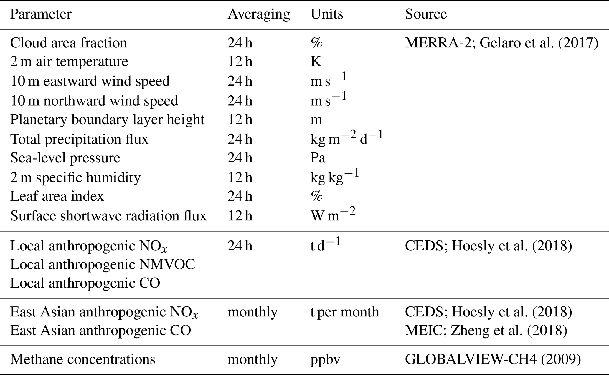
Daily observations from the TOAR dataset spanning 2000–2015 were paired with MERRA-2 meteorological reanalysis data (Gelaro et al., 2017), anthropogenic emissions data from the Community Emissions Data System (CEDS) inventory (Hoesly et al., 2018), monthly East Asian anthropogenic emissions (Hoesly et al., 2018, Zheng et al., 2018), and monthly methane concentrations (GLOBALVIEW-CH4, 2009). Details regarding these parameters are provided in Table 1. Meteorological variables that were considered O3 covariates largely follow Li et al. (2019). Local anthropogenic emissions (Hoesly et al., 2018) included nitrogen oxides (NOx), non-methane volatile organic carbon (NMVOC; includes total weight of all species), and carbon monoxide (CO). Since emissions from East Asia have a large impact on North American ground-level O3 concentrations (Liang et al., 2018) and have dramatically changed in recent decades (Zheng et al., 2018), monthly total emissions from all East Asian countries (i.e., China, Japan, South Korea, North Korea, and Mongolia) were included as an input. Emissions from all East Asian countries were retrieved from the CEDS inventory, with the exception of Chinese emissions, which were retrieved from the Multi-resolution Emission Inventory for China (MEIC) inventory (Zheng et al., 2018). As the last year included in the CEDS inventory is 2014, anthropogenic emissions for 2014 were repeated for 2015. To incorporate geographical differences and long-term drivers not included as input, several fixed-effect parameters were also used as input, including latitude, longitude, and year. A single input into each ANN consists of all the variables described above, which are paired in space and time to an observation retrieved from the TOAR database. Finally, all input data were normalized by subtracting the mean and dividing by the standard deviation of the training dataset.
Prior to model training, the complete dataset was divided into three components – training, validation, and testing. The training dataset is used to iteratively tune the coefficients in the ANN, the validation dataset is used to ensure the training process does not over-fit the ANN parameters to match the training dataset, and the testing dataset is used to evaluate how well the trained model performs. To compile these components, all available data in a given month were collected and 3 random, consecutive days were removed for validation, and 4 random, consecutive days were removed for testing. The remaining days became the training dataset. Overall, the size of the training dataset (i.e., the number of compiled inputs) eclipsed 5 million values; therefore, the number of trainable parameters was nearly 4 orders of magnitude smaller. The optimization of all coefficients at each node in the ANN is accomplished through stochastic gradient descent (SGD) optimization. SGD consists of (a) taking mini-batches of the training dataset, (b) estimating the gradient of all coefficients relative to the known output, (c) taking a small iterative step towards an optimal solution, (d) repeating with a new mini-batch of the training dataset, and (e) repeating steps (a)–(d) until the entire training dataset has been fed through the network. Proceeding through steps (a)-(e) is referred to as an epoch, and network training proceeds through multiple epochs. In total, we used the Adam optimizer (Kingma and Ba, 2015), with a learning rate of 0.001 (i.e., the size of step (c)), a decay factor of 0.9 (i.e., a shrinking of the step (c) size), and a mean-squared error target cost-function. Each ANN was trained for 3000 epochs, with a shuffling of the training data between each epoch. Through monitoring of the model training using the validation dataset, it was determined that 3000 epochs were sufficient to optimize the system without over-fitting.
To quantify the added benefit of the ANN over a simplified model, a comparison with results from a MLR is included. In addition, since exposure mostly occurs at unobserved locations, and all of the model training explained thus far is only evaluated at observed locations (i.e., from the TOAR database), we added an additional step to test our methods. In short, we performed several CTM simulations and sampled the daily-level CTM predictions of each metric at all available monitoring locations, generating what we refer to as a “pseudo-observational dataset”. We then followed the same machine learning process described above, except using the pseudo-observational dataset and four newly trained ANNs, to predict the population-weighted (MDA1/MDA8) and agriculture-weighted (M12/AOT40) exposure values estimated by the CTM. Through this process, we can assess the network's ability to predict total exposure through the exclusive use of sparse measurements.
2.3 Chemical-transport modeling
GEOS-Chem was used to generate ground-level CTM predictions of O3 (v11-01; http://www.geos-chem.org, last access: 5 February 2020; Bey et al., 2001). A nested version of the model at horizontal resolution, driven by native-resolution MERRA-2 meteorology and fed varying boundary conditions, was utilized to simulate O3 throughout the continental United States for the years 2000, 2003, 2005, 2007, 2010, 2012, and 2014. The model includes comprehensive gas chemistry, coupled to an aerosol module that includes sulfate–nitrate–ammonium chemistry (Park et al., 2004; Pye et al., 2009), primary carbonaceous aerosols (Park et al., 2003), mineral dust (Fairlie et al., 2007), and sea salt (Jaegle et al., 2011), with aerosol thermodynamics simulated using ISORROPIA II (Fountoukis and Nenes, 2007). Global anthropogenic emissions come from the CEDS inventory (Hoesly et al., 2018) and were processed through the Harvard–NASA Emission Component (HEMCO; Keller et al., 2014). All nested simulations featured a 2-month spin-up, each O3 metric was calculated at local time, and ground-level concentrations (10 m) from the first level of the GEOS-Chem output were calculated using the methods described in Sect. 3 of Zhang et al. (2012).
2.4 Calculation of metric trends
Trends of all metrics are presented both spatially and weighted towards the subject of interest (i.e., population-weighted or agriculture-weighted). Since the metrics considered here are based on long-term exposure, all trends were assessed at the annual timescale (i.e., one data point, either grid cell or a population-/agriculture-weighted value) using a linear least-squares regression. To calculate population-weighted exposure concentrations, we used population data from the 2017 revisions to the UN Population Division (United Nations, 2017), distributed to grid cells using population density data from the Gridded Population of the World (GPW) version 4 (CIESIN, 2016). Agriculture-weighted exposure concentrations were calculated using crop production and density data from the Food and Agricultural Organization datasets (FAO, 2010).
We also accounted for short-term variability in metric trends by modeling meteorologically adjusted predictions of each metric. To evaluate the ANNs' ability to complete this task, we performed CTM simulations of 2003, 2005, 2007, 2010, 2012, and 2014 using meteorological conditions from each respective year, but frozen anthropogenic emissions and methane concentrations from 2000. We then used the previously trained ANNs (i.e., the ANNs generated using the pseudo-observational data) to predict the population-weighted and agriculture-weighted exposure metrics from these CTM sensitivity simulations. Finally, we compared the CTM- and ANN-predicted trends attributed to meteorology between 2000 and 2015. This enabled us to evaluate how well the ANN can meteorologically adjust exposure trends. From there, the same methods were applied using the ANNs trained with the TOAR data to estimate meteorologically adjusted trends of the population-weighted and agriculture-weighted exposure metrics. Specifically, all variables were held frozen at 2000 values, except for the MERRA-2 meteorological conditions.
2.5 Calculation of human-health and crop-yield impacts
Human-health impacts were quantified using the exposure–response relationships and averaging metrics reported by J2009 and T2016. Both epidemiological studies found a significant relationship between exposure to long-term O3 and premature respiratory mortality. Respiratory impacts are the lone end point considered here since they are the most common impact reported by the community. However, T2016 and several other studies (Jerrett et al., 2013; Crouse et al., 2015; Cakmak et al., 2016; Lim et al., 2019) reported a significant relationship between long-term O3 exposure and other mortality end points, such as cardiovascular disease.
Impact assessments for human health generally report results as the estimated number of premature mortalities attributable to long-term exposure. However, these results can often be driven by non-exposure variables, such as changes in population count (Cohen et al., 2017), baseline mortality rates (Cohen et al., 2017), and population aging (Apte et al., 2018). To eliminate the influence of changes in the total population count on net impacts, we normalized our results and report estimated health impacts as premature mortalities per 100 000 people attributable to long-term O3 exposure. We also illustrate the percent contributions of each variable (i.e., population aging, changes in baseline mortality rates, and exposure) on the net health impact calculations.
Normalized premature mortalities attributable to long-term O3 exposure were calculated as follows.
Here TMREL is the theoretical minimum risk exposure level, ΔX is the predicted long-term O3 exposure concentration above the TMREL, β is the exposure–response factor, HR is the hazard ratio reported by the epidemiological study, ΔY is 10 ppb in both epidemiological studies, AF is the attributable fraction of the disease burden attributable to long-term O3 exposure, y0 is the cause-specific, age-binned baseline mortality rate, population is the age-binned population count, i is the age bin index, ΔMort is the estimated number of cause-specific, age-binned premature mortalities, n is the number of age bins, and Normalized Mort is the estimated number of cause-specific premature mortalities per 100 000 people attributable to long-term O3 exposure. Baseline mortality rates were retrieved from the 2017 GBD (Global Burden of Disease) project (Stanaway et al., 2018) and mapped to best match the ICD-10 (International Statistical Classification of Diseases and Related Health Problems) codes reported in T2016. The hazard ratio for respiratory diseases was 1.040 (95 % CI: 1.013, 1.067) and 1.12 (95 % CI: 1.08, 1.16) in J2009 and T2016, respectively. The TMRELs used were 33.3 ppb when using the J2009 averaging metric and 26.7 ppb when using the T2016 averaging metric, as reported by each epidemiological study.
We report agriculture (maize, soybean, and wheat) impacts in terms of a national relative yield loss (RYL) due to long-term O3 exposure. We utilized the concentration–response function and RYL methods outlined in Van Dingenen et al. (2009), as summarized below.
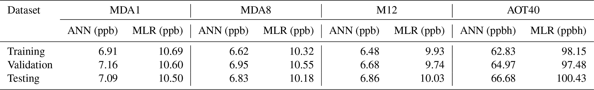
Table 2Daily-level training, validation, and testing performance metrics (RMSE) of the ANN using GEOS-Chem sampled data at TOAR locations compared to a multiple linear regression model. Note ppbh denotes parts per billion-hour.
3.1 Artificial neural network training and evaluation
We began our evaluation using the pseudo-observational dataset derived from daily GEOS-Chem output sampled at all available monitoring locations. From there, we used this dataset to train four ANNs (i.e., one for each metric) and attempted to recreate the original GEOS-Chem output. Through this process, we attempted to determine the strength of an ANN in reconstructing complete exposure maps using sparse observation data. The RMSE results from the initial training and validation datasets were similar (Table 2), indicating that the network was not over-fitting and generalized the system well. When compared to a MLR, the RMSE testing results were ∼33 % lower, demonstrating the added benefit of the ANN (Table 2). Population-weighted and agriculture-weighted exposure estimates from the ANN closely matched the predictions from GEOS-Chem (red vs. blue in Fig. 1) for all metrics and featured a high coefficient of correlation (insets in Fig. 1). An exception was the marginal high bias of the AOT40 metrics for wheat early in the time series. These small deviations were due to a few factors. First, regions of dense agriculture production are limited and generally located in areas with fewer monitors, thus limiting the extent of model training. Second, the AOT40 metric is an accumulation index, which can lead to the amplification of small biases. Separately, we also found the ANN to perform well when meteorologically adjusting the predicted exposure trends (i.e., the short-term trends attributable to meteorology; see insets and green vs. yellow lines in Fig. 1). In total, the ANN was able to reproduce the complete exposure predictions with high fidelity, as estimated by GEOS-Chem, using information strictly from monitoring locations.

Figure 1Red – GEOS-Chem (GC) simulated values of all metrics. Blue – ANN predictions of GC using daily samples from the GEOS-Chem simulations at all available monitoring locations. Green – meteorological trend simulated by GEOS-Chem with all input frozen at 2000 levels, with the exception of meteorological variables. Yellow – ANN prediction of GC-MET (green) using the previously trained (i.e., blue) neural networks. Inset within each panel is the coefficient of correlation for the GC–ANN and GC-MET–ANN-MET time series.
Table 3Daily-level training, validation, and testing performance metrics (RMSE) of the ANN using TOAR observations compared to a multiple linear regression model. Note that ppbh denotes parts per billion-hour.

With confidence in the overall framework, we then trained new ANNs using daily 2000–2015 observations from the TOAR database. Little difference between the training, validation, and testing performance metrics indicated that each ANN was not over-fitting to the training dataset (Table 3). In addition, we again found the ANN to perform ∼30 % better than a MLR model (Table 3). When compared to the original TOAR database, we found high accuracy between each ANN-predicted long-term metric and the original observations (Figs. S1–S4; Table S1 in the Supplement). The RMSE of the MDA1 and MDA8 predictions ranged from 3.1 to 4.4 and 2.3 to 3.9 ppb, respectively (Table S1). The r2 of the two metrics ranged from 0.77 to 0.84 and 0.74 to 0.82. Similar levels of bias (RMSE) and correlation (r2) were found when comparing the long-term agriculture metrics (Table S1).
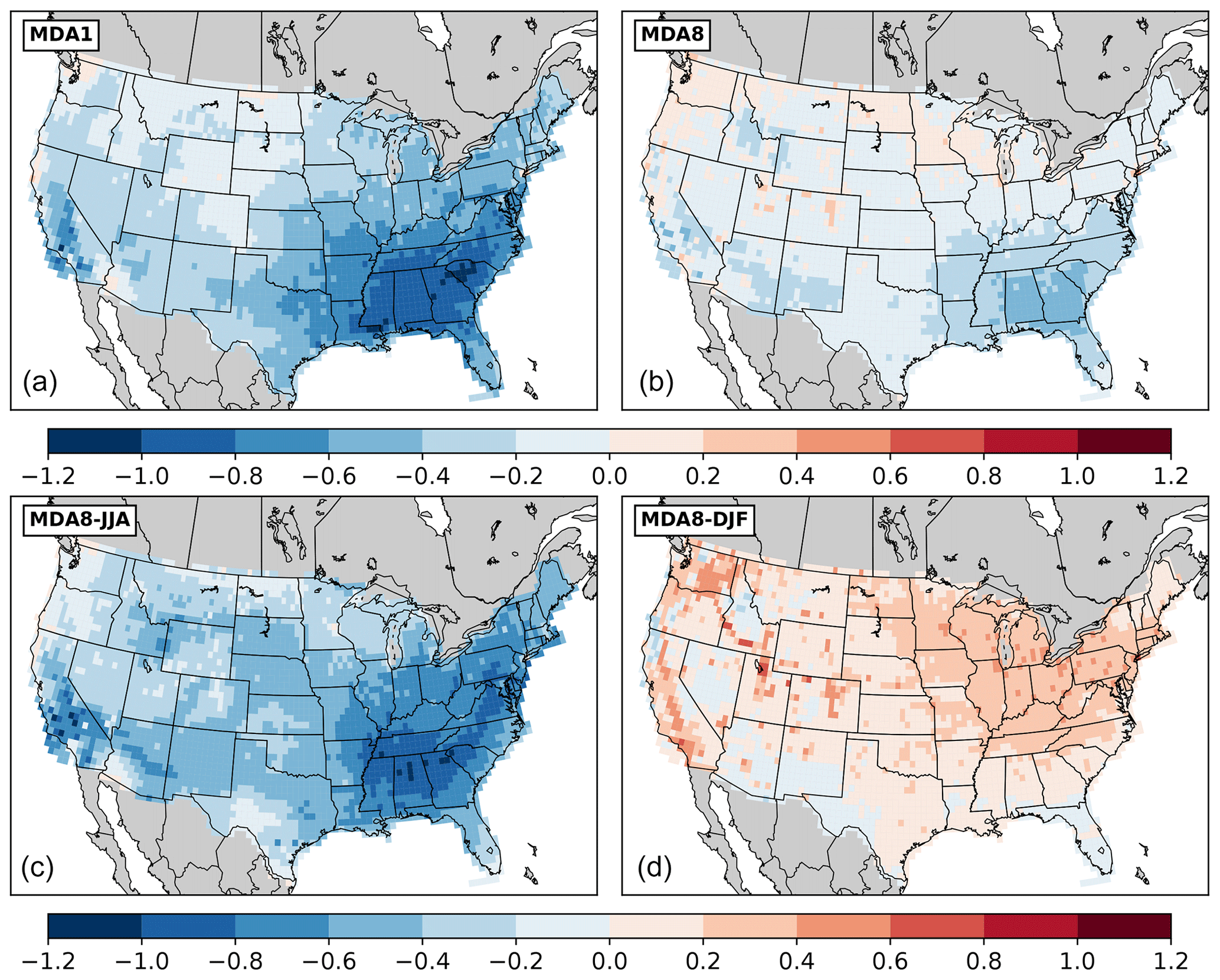
Figure 2Trends of the MDA1 (a; ppb yr−1) and MDA8 (b; ppb yr−1) health metrics from 2000 to 2015. Trends of MDA8-JJA (c; ppb yr−1) and MDA8-DJF (d; ppb yr−1) from 2000 to 2015. The p values from these trends can be found in Fig. S5.
3.2 Magnitude and trends of long-term O3 exposure metrics
3.2.1 Human-health-relevant metrics
The MDA1 metric featured large reductions throughout the study period, with downward trends exceeding 1 ppb yr−1 in the Southeast and in portions of California (Fig. 2). As a result, exposure throughout this period simultaneously decreased. The national population-weighted exposure concentration peaked in 2002 at 55.9 ppb, reached a minimum of 48.2 ppb in 2014, and featured sizable year-to-year fluctuations due to inter-annual variation (Fig. 3). From 2000 to 2015, the national population-weighted exposure concentration of the MDA1 metric featured an annual decrease of 0.43 [95 % CI: 0.28, 0.57] ppb yr−1 (Table S4). After adjusting for meteorology, the trend changed to −0.41 [95 % CI: −0.35, −0.47] ppb yr−1. The similar mean values of these two trends suggest that nearly all of the MDA1 reductions are due to non-meteorological drivers (i.e., emission changes, intercontinental transport, methane). Changes in exposure featured an east–west divide, with population-weighted exposure concentrations decreasing by 0.49 [95 % CI: 0.28, 0.69] ppb yr−1 in the east and 0.31 [95 % CI: 0.21, 0.41] ppb yr−1 in the west (Fig. 3, Table S4).
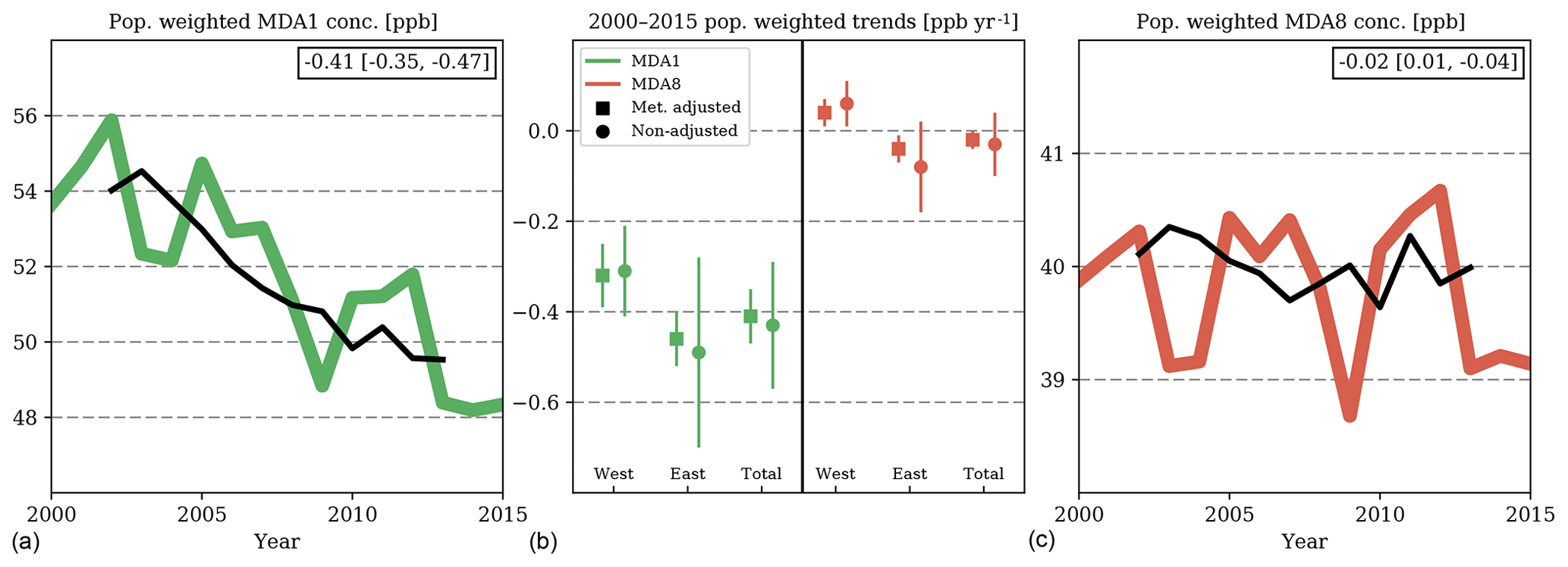
Figure 3(a) Population-weighted exposure concentrations of the MDA1 human-health metric from 2000 to 2015. The meteorologically adjusted trend is in black with the slope in the inset. (b) The 2000–2015 population-weighted trends (ppb yr−1) of the MDA1 (green) and MDA8 (red) metrics. The west–east divide is made along the 95∘ W meridian and the whiskers span the 95 % confidence interval. (c) Population-weighted exposure concentrations of the MDA8 human-health metric from 2000 to 2015. The meteorologically adjusted trend is in black with the slope in the inset. Tabulated values of these plots can be found in Table S2 and S4.
In contrast, the MDA8 metric featured more modest decreases in the Southeast USA and scattered areas with increasing trends (Fig. 2). This divergence between the two human-health metrics is due to the different averaging periods (i.e., the traditional “ozone season” vs. an annual average). If only summer months were considered when calculating the MDA8 metric (i.e., MDA8-JJA), the two trends would be spatially and quantitatively consistent (Fig. 2). However, O3 increases during the winter months (i.e., MDA8-DJF) partially compensated for the summer decreases, resulting in no discernable trend for the national population-weighted MDA8 metric (Fig. 3). After adjusting for meteorology, the national population-weighted MDA8 trend from 2000 to 2015 is −0.02 [95 % CI: 0.01, −0.04] ppb yr−1 (Fig. 3). Similar to the MDA1 metric, trends featured an east–west divide. It is interesting to note that the western MDA8 trends were slightly positive and the eastern MDA8 trends were slightly negative (Table S4). Separately, prior studies (e.g., Bloomer et al., 2010; Cooper et al., 2012; Parrish et al., 2012; Clifton et al., 2014; Simon et al., 2015; Strode et al., 2015; Fleming et al., 2018) have highlighted the existence of a seasonal shift in the distribution of O3 concentrations throughout the United States. We find that these shifts have not only manifested in contrasting seasonal trends (i.e., summer decreases vs. winter increases), but have also led to changes in the dominant months of O3 exposure. For example, the population-weighted exposure concentrations during the spring and summer months (MDA8-MAM vs. MDA8-JJA) were nearly equivalent from 2013 to 2015 (Table S2).
It should be noted that comparing previously reported seasonal trends of O3 is difficult due to varying study periods, averaging metrics, and selection of monitoring networks. Oftentimes, rural locations are highlighted, enabling the isolation of trends in background O3 concentrations or the minimization of the influence of nearby changes in anthropogenic emissions (e.g., Jaffe and Ray, 2007; Cooper et al., 2012; Jaffe et al., 2018). These study-specific choices can effect conclusions. For example, Simon et al. (2015) report that rural O3 monitors more often feature statistically significant decreases in national mean MDA8 O3 during summer months and urban O3 monitors more often feature statistically significant increases in national mean MDA8 O3 during winter months. For this study, since our focus is on changes in exposure, we incorporate all available observational data, including monitors in urban cores. As such, when compared to prior studies, our conclusions regarding O3 trends may be different.
Cooper et al. (2012), using rural monitoring data spanning 1990–2010, reported a −0.45 and a +0.10 ppb yr−1 trend in daytime O3 during summer months for the eastern and western USA, respectively. However, both trends featured wide ranges. Jaffe et al. (2018), using a limited number of high-elevation, rural monitoring sites, reported decreasing trends of median summertime O3 between 2000 and 2016 at most analyzed locations, with stronger decreases in the east than west (∼1 ppb yr−1 vs. ∼0.5 ppbẏr). Lin et al. (2017) also used rural monitoring data, but increased the coverage to include 1988–2014 and found a 0.4–0.8 ppb yr−1 decreasing trend of median MDA8-JJA concentrations in the eastern USA and mixed trends in the west. Fleming et al. (2018) incorporated both urban and nonurban monitors and showed that the observed magnitude of several warm season human-health ozone metrics is similar for North American urban and nonurban sites and that the trends are only slightly smaller for the urban areas. Broadly, we also found a dramatic divide between east and west summertime O3 exposure trends, but our results did feature some differences from prior studies. For example, our exposure-focused (i.e., population-weighted) estimates of eastern USA trends are similar to the mean reported by Cooper et al. (2012) and on the low end of that reported by Lin et al. (2017). We also found a consistent decreasing trend in western MDA8-JJA exposure, as well as smaller levels of trend uncertainty (Table S4).
Cooper et al. (2012) also reported a uniform east and west increase in rural wintertime O3 concentrations of 0.12 ppb yr−1. However, the exclusive selection of rural monitors precludes the extrapolation of those results to estimate exposure trends. This is well illustrated by Simon et al. (2015), who used an extensive network of 1998–2013 observations to show that there was a strong rural–urban divide in mean winter O3 trends, with increasing trends more prevalent in urban areas. Indeed, when compared to Cooper et al. (2012), we found a much stronger trend increase in MDA8-DJF exposure (Table S4). Our results indicate that the national trend in MDA8-DJF exposure was +0.33 [95 % CI: 0.37, 0.28] ppb yr−1 (Table S4), with a near-uniform increase in both the east and west.
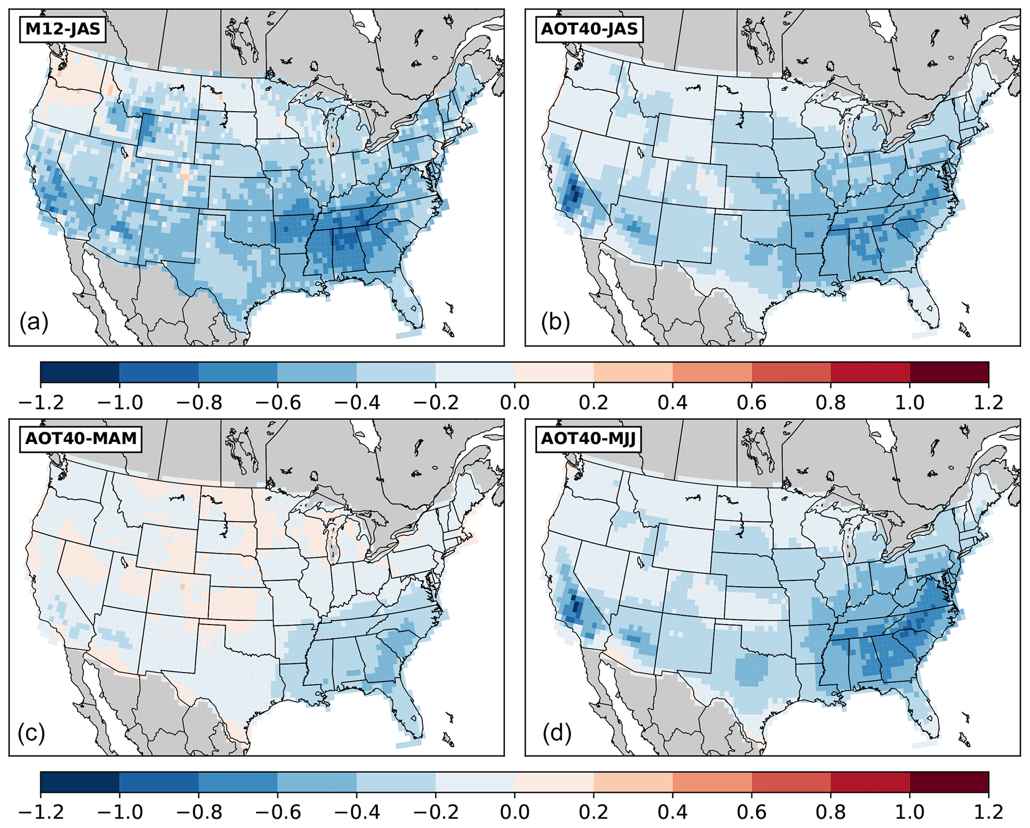
Figure 4Trends of the M12 (a; ppb yr−1) and AOT40 (b, c, d; ppmh yr−1) agriculture metrics from 2000 to 2015. Note: JAS: July–September; MAM: March–May; MJJ: May–July. The p values from these trends can be found in Fig. S6.
3.2.2 Crop-loss-relevant metrics
Since the averaging months for crop-loss metrics are dependent on crop variety, the magnitude and trends can feature distinct patterns (Table S3). All maize and soybean metrics envelop the months of July–September. As such, and consistent with the MDA1 results, this averaging period yielded widespread decreases for both the M12 and AOT40 metrics, with the strongest reductions in the southeast and California (Fig. 4a, b). However, both of these crops are predominantly grown in the Midwest and Great Plains (Fig. S7). These regions generally experienced smaller trend reductions. Nationally, the agriculture-weighted trends of the M12 metric for maize and soybeans were −0.35 [95 % CI: −0.17, −0.54] ppb yr−1 and −0.39 [95 % CI: −0.19, −0.59] ppb yr−1 (Fig. 5; Table S4). The agriculture-weighted trends of the AOT40 metric for maize and soybeans were −0.35 [95 % CI: −0.18, −0.51] ppmh yr−1 and −0.39 [95 % CI: −0.21, −0.56] ppmh yr−1 (Fig. 5; Table S4). After adjusting for meteorology, the mean trend for both metric and crop pairings was reduced marginally, suggesting that meteorological factors played a small role in the net trends from 2000 to 2015 (Fig. 5b).
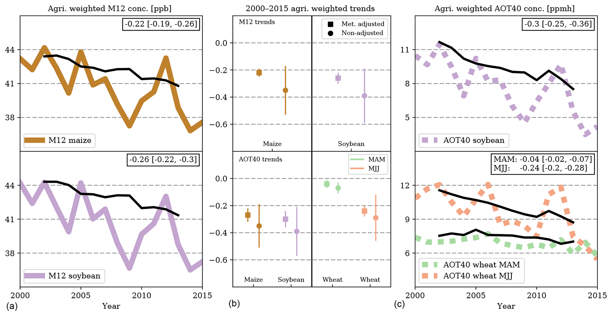
Figure 5(a) Agriculture-weighted exposure concentrations of the M12 agriculture metrics from 2000 to 2015. The meteorologically adjusted trend of each metric is in black with the slope in the inset. (b) The 2000–2015 agriculture-weighted trends (ppb yr−1 for M12, ppmh yr−1 for AOT40) of the M12 and AOT40 metrics. The whiskers span the 95 % confidence interval. (c) Agriculture-weighted exposure concentrations of the AOT40 agriculture metrics from 2000 to 2015 (trends of AOT40 soybean and AOT40 maize are nearly equivalent). The meteorologically adjusted trend of each metric is in black with the slope in the inset. Note: variable averaging periods are considered, reflecting differences in crop harvest seasons. Tabulated values of the left and right plots can be found in Tables S3 and S4.
Both agriculture-weighted AOT40 averaging periods for wheat (MAM and MJJ) featured decreasing, but considerably different, trends (Fig. 5, bottom panels). These trend differences again highlight the seasonal shift in O3 concentrations. From 2000 to 2006, the AOT40-MJJ wheat metric was ∼40 %–60 % higher than the AOT40-MAM wheat metric (Table S3). However, by 2014, both metrics were nearly equal. The 40 ppb accumulation threshold applied in the AOT40 calculation also amplifies this convergence. Towards the end of the study period, mean daytime O3 concentrations in the Midwest and Great Plains had decreased sufficiently for the two metrics to nearly intersect.
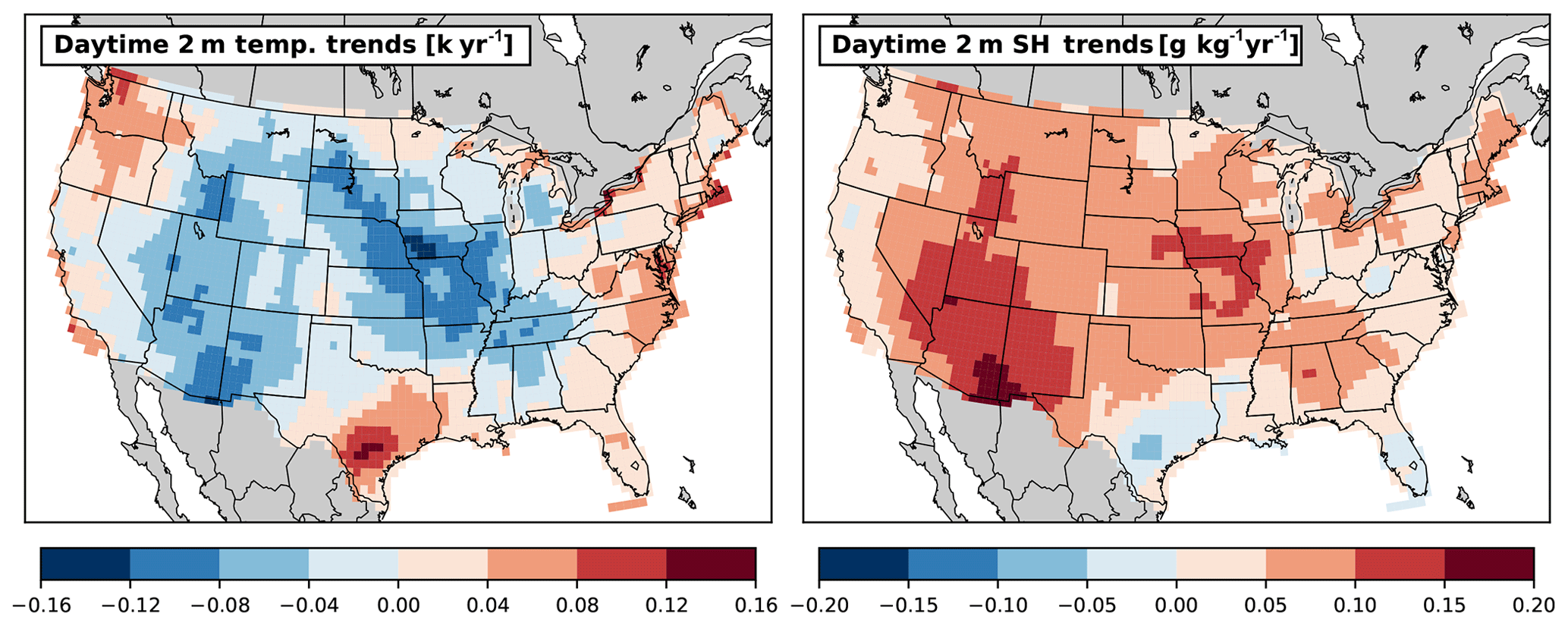
Figure 6Annual trends in the daytime 2 m temperature and daytime 2 m specific humidity from 2000 to 2015.
We posit that the influence of meteorology on the agriculture-weighted trends, as indicated by the marginal difference in the mean of the meteorologically adjusted and non-adjusted trends, is primarily due to two factors. Prior analysis has shown that two important meteorological variables influencing O3 include temperature and humidity (Camalier et al., 2007; Jacob and Winner, 2009). The temperature–O3 mechanism is a function of increasing temperatures promoting peroxyacetyl nitrate decomposition (leading to ozone increases near NOx source regions, but decreases in remote areas; Doherty et al., 2013) and increases in isoprene emissions. The humidity–O3 mechanism is a function of increasing water vapor concentrations, promoting O3 chemical destruction. According to the MERRA-2 reanalysis product, the Midwest and Great Plains regions featured both decreasing trends in daytime 2 m temperature and increasing trends in daytime 2 m specific humidity (Fig. 6). In addition, acute O3 episodes are notably sensitive to particular meteorological variables (Russell et al., 2016; Fix et al., 2018), such as temperature, providing an environment where meteorological variability can disproportionately influence the magnitude of AOT40 values.
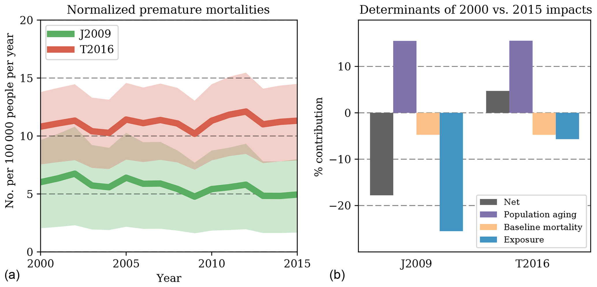
Figure 7(a) Annual estimates of normalized premature mortalities (number per 100 000 people per year) attributable to long-term O3 exposure using the MDA1 and MDA8 averaging metrics and exposure–response function from J2009 and T2016, respectively. The shaded region reflects the confidence interval reported in each underlying epidemiological study. (b) The 2000 vs. 2015 percent contributions of population aging, changing baseline mortality rates, and long-term O3 exposure to net normalized premature mortalities using the MDA1 and MDA8 averaging metrics and exposure–response function from J2009 and T2016, respectively. Tabulated values of (a) can be found in Table S5.
3.3 Estimates of long-term O3 exposure impacts
3.3.1 Human health
Human-health impacts, reported as the estimated number of premature respiratory mortalities attributable to long-term O3 exposure per 100 000 people, were strongly dependent on the choice of exposure–response relationship (Fig. 7). First, the T2016 results reported nearly double the estimated human-health impacts attributable to long-term O3 exposure. For example, in 2010, the J2009 and T2016 estimated impacts were ∼5.4 [95 % CI: 1.8, 8.7] and ∼11.3 [95 % CI: 7.9, 14.5] premature mortalities per 100 000 people, respectively. Second, the diverging trends of the two exposure metrics (Fig. 3) are reflected in the estimated impacts (Fig. 7). Between 2000 and 2015, the MDA1 population-weighted exposure concentration decreased from ∼53.7 to ∼48.3 ppb (Table S2). As a result, the estimated human-health impacts using the J2009 parameters decreased from ∼6.0 [95 % CI: 2.0, 9.7] to ∼5.0 [95 % CI: 1.7, 8.0] premature mortalities per 100 000 people (Table S5). In contrast, the MDA8 population-weighted exposure concentration decreased from ∼39.9 to ∼39.1 ppb, yet the impacts using the T2016 parameters increased from ∼10.8 [95 % CI: 7.6, 13.8] to ∼11.3 [95 % CI: 7.9, 14.5] premature mortalities per 100 000 people (Fig. 7 and Table S5). These differences in estimated impacts are not only due to changes in exposure. Over this period, an aging population structure promoted increased susceptibility to O3 impacts. In addition, depending on the age bin, baseline mortality rates for respiratory diseases either marginally decreased or remained approximately stable.
While impacts due to changes in exposure for both metrics decreased between these end points, albeit by different magnitudes (blue bars in Fig. 7b; −25.5 % vs. −5.7 %), these other determinants played a strong role in modulating the estimated impact trends (Fig. 7b). The net changes in 2015 vs. 2000 normalized human-health impacts using the J2009 and T2016 exposure–response relationships and averaging metrics were −17.8 % and +4.7 %, respectively (black bars in Fig. 7b). In both calculations, an aging population structure substantially eliminated much of the gains from exposure decreases (+15.5 %). Changing baseline mortality rates were more modest, decreasing both calculations by 4.7 %.
The differences in estimated human-health impacts when using the J2009 and T2016 exposure–response relationship and averaging metrics reported here are consistent with prior studies (Malley et al., 2017; Seltzer et al., 2018; Shindell et al., 2018). That is, the estimated human-health impacts when using the T2016 exposure–response relationship and averaging metric are considerably higher than the results computed when using the J2009 parameters. However, to our knowledge, the historical evolving differences between the two have yet to be shown. For example, the T2016 results were ∼80 % higher than the J2009 results in 2000 (Table S5). By 2008, the T2016 results were nearly double the J2009 results, and this difference continued to grow over time (∼130 % in 2015).
Between 2000 and 2015, our net estimated premature mortalities attributable to long-term O3 exposure in the USA ranged from ∼14 500 to 19 200 when using the J2009 parameters and from ∼29 800 to 37 600 when using the T2016 parameters. These results are lower than analogous prior studies that are based solely on CTM estimates of O3 exposure. An exception is Zhang et al. (2018), who found comparable results when using the J2009 epidemiological study. However, Zhang et al. (2018) report a 13 % increase in premature mortalities attributable to long-term O3 exposure in the United States between 1990 and 2010, despite O3 decreases. We find a ∼6.7 % decrease in premature mortalities attributable to long-term O3 exposure, albeit over 2000–2015. This is likely due to the dramatic decreases in O3 precursor emissions that occurred post-2000 (Xing et al., 2013; Simon et al., 2015).
3.3.2 Crop loss
Agriculture impacts for each of the crop varieties considered here decreased from 2000 to 2015 (Fig. 8). When using the M12 metric, the estimated national RYL values for maize and soybeans in 2000 were 4.6 % and 16.3 %, respectively (Fig. 8 and Table S5). These values decreased to 2.9 % and 11.2 % in 2015. When using the AOT40 metric, the estimated national RYL values for maize, soybeans, and wheat for the year 2000 were 3.4 %, 11.9 %, and 12.1 %, respectively. By 2015, these RYL values dropped to 1.6 %, 4.8 %, and 9.4 %, respectively. Broadly, these estimated agriculture yield impacts are comparable to the global “ozone yield gaps” (i.e., RYL) modeled by Mills et al. (2018a), who considered the flux-based, stomatal uptake of O3 for each crop.
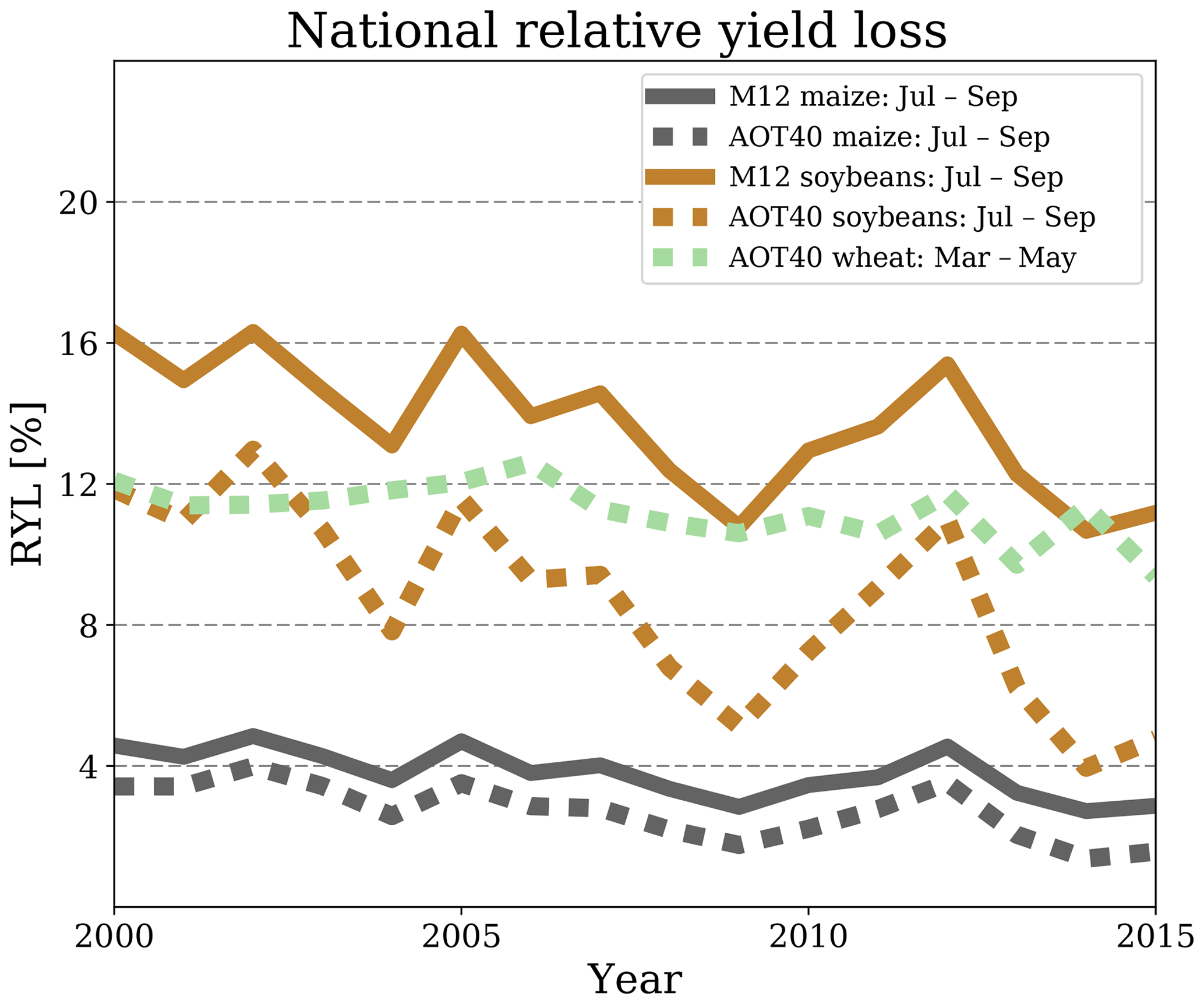
Figure 8Estimates of the national relative yield loss for a variety of commercial crops using ANN-calculated exposure metrics. Tabulated values of this plot can be found in Table S5.
Several other characteristics are consistent among all of the crop varieties and metric combinations considered here. For one, estimated RYL featured sizable inter-annual variability, indicating that the impacts calculated from a single year might not be representative of a particular period. For example, the RYL for soybeans, when using the AOT40 metric, increased from 7.8 % in 2004 to 11.6 % in 2005 – a nearly ∼50 % increase. Second, similar to Van Dingenen et al. (2009) and Lapina et al. (2016), impacts were consistently higher when utilizing the M12 metric and the associated concentration–response functions. These differences also became amplified over time. The RYL for soybeans in 2000 using the M12 metric (16.3 %) was ∼37 % higher than the RYL using the AOT40 metric (11.9 %). This difference increased to ∼135 % (11.2 % vs. 4.8 %) by 2015 (Table S5). These diverging trends occur for two reasons. First, the daytime O3 concentrations approached the AOT40 threshold of 40 ppb post-2007 (Table S3). This decrease precipitated disproportional improvements in AOT40-calculated RYL. Second, and to a lesser degree, the slopes of the two soybean concentration–response functions are different (Fig. S8).
Studies quantifying the health impacts attributable to long-term PM2.5 exposure oftentimes use higher-resolution products (e.g., ) that harness satellite data (e.g., Apte et al., 2015; Cohen et al., 2017; van Donkelaar et al., 2019). However, a number of complications prevent such products for surface O3 (Duncan et al., 2014). Regardless, we believe this product is of sufficient resolution to estimate long-term O3 exposure for a number of reasons. First, O3 features a residence time on the order of hours to days in the lower troposphere and in urban environments (Parrish et al., 2012; Monks et al., 2015), providing sufficient time for localized and regional mixing. Second, unlike short-term O3 exposure, long-term O3 exposure is less sensitive to singular events that are more heterogeneous in space and time. Third, regional CTM studies report only marginal differences in O3 concentrations and estimated impacts when scaling from 12 km to resolutions comparable to those in this analysis (Punger and West, 2013; Gan et al., 2016).
In terms of impacts, there is evidence that O3 affects more than what was presented here. For example, several epidemiological studies suggest that human-health impacts may extend to cardiovascular mortality (Jerrett et al., 2013; Crouse et al., 2015; Cakmak et al., 2016; Turner et al., 2016; Lim et al., 2019). Separately, our analysis applied a log-linear exposure–response function when performing the human-health calculations since it is most common method applied in the community. There is evidence that this relationship may instead be linear (Di et al., 2017). For agriculture, the exposure–response functions utilized here are “pooled” from studies featuring a limited number of cultivars grown in the USA and Europe (Van Dingenen et al., 2009). While considered reliably representative of the commonly grown cultivar population in these regions, extrapolation of these relationships to the national level may introduce additional uncertainty. In addition, the methodology selected here does not take into account changes in plant conditions that may limit or exacerbate conditions which influence the opening of stomata and the ability of a plant to uptake O3, such as temperature and soil moisture. The results presented here also demonstrate the need for additional epidemiological studies to test the utility of common averaging metrics that are used when estimating health impacts. Specifically, clarity is needed regarding whether long-term O3 health impacts are more sensitive to peak averaged (i.e., the MDA1 metric) or annually averaged (i.e., the MDA8 metric) O3 exposure.
Finally, long-term trends of O3 are driven by a number of mechanisms, including intercontinental transport (Fiore et al., 2009; Lin et al., 2012, 2017) and methane concentrations (Fiore et al., 2002; Shindell et al., 2017; Lin et al., 2017). For example, Lin et al. (2015) conclude that rising Asian emissions and global methane have played a key role in the increase in western USA springtime O3 from 1995 to 2014. These drivers merit additional study, with an emphasis on exploring seasonal differences that influence impact metrics. Furthermore, inclusion of observations from the most recent years (i.e., 2015–2017) should be targeted. Since Chinese emissions of NOx peaked in 2012 (Zheng et al., 2018), our current and future estimates of intercontinental transport influences on background O3 might warrant revisiting.
Through the application of artificial neural networks, we empirically model the magnitude and trends of long-term (i.e., seasonal, annual) ambient O3 over the continental United States from 2000 to 2015. We then used these estimates of long-term O3 exposure to generate a measurement-based assessment of impacts on human health and crop yields. All metrics with averaging periods spanning the traditional O3 season (i.e., warm months) featured peak exposure in 2002, with net decreases over the course of the study period. For example, the population-weighted, April–September average of the daily 1 h maximum O3 concentration (i.e., MDA1 from Jerrett et al., 2009) decreased by 0.43 [95 % CI: 0.28, 0.57] ppb yr−1 between 2000 and 2015. In contrast, there was little change in the population-weighted, annual average of the maximum daily 8 h average O3 concentration (i.e., MDA8 from Turner et al., 2016) between 2000 and 2015. There were compensating seasonal effects, with wintertime O3 increases and summertime O3 decreases, yielding a net population-weighted trend of −0.03 [95 % CI: 0.04, −0.10] ppb yr−1. Human-health metric trends also featured an east–west divide, with stronger decreases in the eastern USA. All agriculture-weighted crop-loss metrics featured decreasing trends over the study period.
Human-health impacts were quantified in terms of the estimated number of premature respiratory mortalities attributable to long-term O3 exposure per 100 000 people. Crop-loss impacts were quantified in terms of the estimated national relative yield loss for a variety of commercial crops. Normalized human-health impact estimates decreased by ∼18 % and increased by ∼5 % when using the Jerrett et al. (2009) and Turner et al. (2016) averaging metrics and parameters, respectively. In both cases, exposure changes and an aging population structure played a substantial role in modulating these trends. When using the M12 metric, the relative yield loss (RYL) due to O3 exposure for maize and soybeans improved by 1.7 % and 5.1 %. When using the AOT40 metric, the net benefits were greater, with the RYL for maize, soybeans, and wheat improving by 1.9 %, 7.1 %, and 2.7 %, respectively. These different responses are mainly due to the daylight O3 concentrations approaching the 40 ppb AOT40 threshold by the end of the study period. Overall, these results provide a measurement-based estimate of long-term O3 exposure over the United States, quantify the historical trends of such exposure, and illustrate how different conclusions regarding historical impacts can be made through the use of varying metrics.
Maps of the O3 exposure metrics used in this study can be accessed by contacting one of the corresponding authors.
The supplement related to this article is available online at: https://doi.org/10.5194/acp-20-1757-2020-supplement.
All authors contributed to the design and/or methodology of the study. KMS applied the methods, analyzed the results, developed all figures/tables, and drafted the initial manuscript. All authors edited and contributed to subsequent drafts of the manuscript.
The authors declare that they have no conflicts of interest.
Karl M. Seltzer was supported by NASA headquarters under the NASA Earth and Space Science Fellowship Program – grant no. 80NSSC17K0354. All O3 observations were retrieved from the TOAR database via the Representational State Transfer (REST) services. Special thanks to the TOAR team/community, particularly Owen Cooper, Martin Schultz, and Sabine Schröder, for compiling all of the observations into a variety of metrics; the MEIC team for providing Chinese anthropogenic emissions; the Duke Compute Cluster for computational resources; and the University of Florida's HiPerGator for computational resources.
This research has been supported by the NASA Earth and Space Science Fellowship Program (grant no. #80NSSC17K0354).
This paper was edited by Pedro Jimenez-Guerrero and reviewed by three anonymous referees.
Abadi, M., Agarwal, A., Barham, P., Brevdo, E., Chen, Z., Citro, C., Corrado, G. S., Davis, A., Dean, J., Devin, M., Ghemawat, S., Goodfellow, I., Harp, A., Irving, G., Isard, M., Jia, Y., Jozefowicz, R., Kaiser, L., Kudlur, M., Levenberg, J., Mane, D., Monga, R., Moore, S., Murray, D., Olah, C., Schuster, M., Shlens, J., Steiner, B., Sutskever, I., Talwar, K., Tucker, P., Vanhoucke, V., Vasudevan, V., Viegas, F., Vinyals, O., Warden, P., Wattenberg, M., Wicke, M., Yu, Y., and Zheng, X.: TensorFlow: Large-Scale Machine Learning on Heterogeneous Distributed Systems, http://arxiv.org/abs/1603.04467 (last access: 5 February 2020), 2015.
Anenberg, S. C., Horowitz, L. W., Tong, D. Q., and West, J. J.: An estimate of the global burden of anthropogenic ozone and fine particulate matter on premature human mortality using atmospheric modeling, Environ. Health Persp., 118, 1189–1195, https://doi.org/10.1289/ehp.0901220, 2010.
Apte, J. S., Marshall, J. D., Cohen, A. J., and Brauer, M.: Addressing Global Mortality from Ambient PM2.5, Environ. Sci. Technol., 49, 8057–8066, https://doi.org/10.1021/acs.est.5b01236, 2015.
Avnery, S., Mauzerall, D. L., Liu, J., and Horowitz, L. W.: Global crop yield reductions due to surface ozone exposure: 1. Year 2000 crop production losses and economic damage, Atmos. Environ., 45, 2284–2296, https://doi.org/10.1016/j.atmosenv.2010.11.045, 2011.
Bell, M. L.: The use of ambient air quality modeling to estimate individual and population exposure for human health research: A case study of ozone in the Northern Georgia Region of the United States, Environ. Int., 32, 586–593, https://doi.org/10.1016/j.envint.2006.01.005, 2006.
Bey, I., Jacob, D. J., Yantosca, R. M., Logan, J. A., Field, B. D., Fiore, A. M., Li, Q., Liu, H. Y., Mickley, L. J., and Schultz, M. G.: Global modeling of tropospheric chemistry with assimilated meteorology: Model description and evaluation, J. Geophys. Res., 106, 23073–23095, https://doi.org/10.1029/2001jd000807, 2001.
Bloomer, B. J., Vinnikov, K. Y., and Dickerson, R. R.: Changes in seasonal and diurnal cycles of ozone and temperature in the eastern U.S., Atmos. Environ., 44, 2543–2551, https://doi.org/10.1016/j.atmosenv.2010.04.031, 2010.
Brauer, M., Lencar, C., Tamburic, L., Koehoorn, M., Demers, P., and Karr, C.: A Cohort Study of Traffic-Related Air Pollution Impacts on Birth Outcomes, Environ. Health Persp., 116, 680–686, https://doi.org/10.1289/ehp.10952, 2008.
Cakmak, S., Hebbern, C., Vanos, J., Crouse, D. L., and Burnett, R.: Ozone exposure and cardiovascular-related mortality in the Canadian Census Health and Environment Cohort (CANCHEC) by spatial synoptic classification zone, Environ. Pollut., 214, 589–599, https://doi.org/10.1016/j.envpol.2016.04.067, 2016.
Camalier, L., Cox, W., and Dolwick, P.: The effects of meteorology on ozone in urban areas and their use in assessing ozone trends, Atmos. Environ., 41, 7127–7137, https://doi.org/10.1016/j.atmosenv.2007.04.061, 2007.
Center for International Earth Science Information Network – CIESIN – Columbia University. Gridded Population of the World, Version 4 (GPWv4): Population Density Adjusted to Match 2015 Revision UN WPP Country Totals, Palisades, NY: NASA Socioeconomic Data and Applications Center (SEDAC); https://doi.org/10.7927/H4HX19NJ, 2016.
Chameides, W. L., Kasibhatla, P. S., Yienger, J., and Levy II, H.: Growth of Continental-Scale Metro-Agro-Plexes, Regional Ozone Pollution, and World Food Production, Science, 264, 74–77, 1994.
Chang, H. H., Zhou, J., and Fuentes, M.: Impact of climate change on ambient ozone level and mortality in Southeastern United States, Int. J. Environ. Res. Pub. He., 7, 2866–2880, https://doi.org/10.3390/ijerph7072866, 2010.
Chang, K.-L., Petropavlovskikh, I., Copper, O. R., Schultz, M. G., and Wang, T.: Regional trend analysis of surface ozone observations from monitoring networks in eastern North America, Europe and East Asia, Elem. Sci. Anthr., 5, https://doi.org/10.1525/elementa.243, 2017.
Chollet, F.: keras, GitHub, available at: https://github.com/fchollet/keras (last access: 5 February 2020), 2015.
Clifton, O. E., Fiore, A. M., Correa, G., Horowitz, L. W., and Naik, V.: Twenty-first century reversal of the surface ozone seasonal cycle over the northeastern United States, Geophys. Res. Lett., 41, 7343–7350, https://doi.org/10.1002/2014GL061378, 2014.
Cohen, A. J., Brauer, M., Burnett, R., Anderson, H. R., Frostad, J., Estep, K., Balakrishnan, K., Brunekreef, B., Dandona, L., Dandona, R., Feigin, V., Freedman, G., Hubbell, B., Jobling, A., Kan, H., Knibbs, L., Liu, Y., Martin, R., Morawska, L., Pope, C. A., Shin, H., Straif, K., Shaddick, G., Thomas, M., van Dingenen, R., van Donkelaar, A., Vos, T., Murray, C. J. L., and Forouzanfar, M. H.: Estimates and 25-year trends of the global burden of disease attributable to ambient air pollution: an analysis of data from the Global Burden of Diseases Study 2015, Lancet, 389, 1907–1918, https://doi.org/10.1016/S0140-6736(17)30505-6, 2017.
Comrie, A. C.: Comparing Neural Networks and Regression Models for Ozone Forecasting, J. Air Waste Manage., 47, 653–663, https://doi.org/10.1080/10473289.1997.10463925, 1997.
Cooper, O. R., Gao, R. S., Tarasick, D., Leblanc, T., and Sweeney, C.: Long-term ozone trends at rural ozone monitoring sites across the United States, 1990-2010, J. Geophys. Res.-Atmos., 117, 1990–2010, https://doi.org/10.1029/2012JD018261, 2012.
Cooper, O. R., Parrish, D. D., Ziemke, J., Balashov, N. V., Cupeiro, M., Galbally, I. E., Gilge, S., Horowitz, L., Jensen, N. R., Lamarque, J.-F., Naik, V., Oltmans, S. J., Schwab, J., Shindell, D. T., Thompson, A. M., Thouret, V., Wang, Y., and Zbinden, R. M.: Global distribution and trends of tropospheric ozone: An observation-based review, Elem. Sci. Anthr., 2, https://doi.org/10.12952/journal.elementa.000029, 2014.
Crouse, D. L., Peters, P. A., Hystad, P., Brook, J. R., van Donkelaar, A., Martin, R. V., Villeneuve, P. J., Jerrett, M., Goldberg, M. S., Arden Pope, C., Brauer, M., Brook, R. D., Robichaud, A., Menard, R., and Burnett, R. T.: Ambient PM2.5, O3, and NO2 exposures and associations with mortality over 16 years of follow-up in the canadian census health and environment cohort (CanCHEC), Environ. Health Persp., 123, 1180–1186, https://doi.org/10.1289/ehp.1409276, 2015.
Di, Q., Rowland, S., Koutrakis, P., and Schwartz, J.: A hybrid model for spatially and temporally resolved ozone exposures in the continental United States, J. Air Waste Manage., 67, 39–52, https://doi.org/10.1080/10962247.2016.1200159, 2017.
Doherty, R. M., Wild, O., Shindell, D. T., Zeng, G., MacKenzie, I. A., Collins, W. J., Fiore, A. M., Stevenson, D. S., Dentener, F. J., Schultz, M. G., Hess, P., Derwent, R. G., and Keating, T. J.: Impacts of climate change on surface ozone and intercontinental ozone pollution: A multi-model study, J. Geophys. Res.-Atmos., 118, 3744–3763, https://doi.org/10.1002/jgrd.50266, 2013.
Duncan, B. N., Prados, A. I., Lamsal, L. N., Liu, Y., Streets, D. G., Gupta, P., Hilsenrath, E., Kahn, R. A., Nielsen, J. E., Beyersdorf, A. J., Burton, S. P., Fiore, A. M., Fishman, J., Henze, D. K., Hostetler, C. A., Krotkov, N. A., Lee, P., Lin, M., Pawson, S., Pfister, G., Pickering, K. E., Pierce, R. B., Yoshida, Y., and Ziemba, L. D.: Satellite data of atmospheric pollution for U.S. air quality applications: Examples of applications, summary of data end-user resources, answers to FAQs, and common mistakes to avoid, Atmos. Environ., 94, 647–662, https://doi.org/10.1016/j.atmosenv.2014.05.061, 2014.
Dutot, A. L., Rynkiewicz, J., Steiner, F. E., and Rude, J.: A 24-h forecast of ozone peaks and exceedance levels using neural classifiers and weather predictions, Environ. Model. Softw., 22, 1261–1269, https://doi.org/10.1016/j.envsoft.2006.08.002, 2007.
Fairlie, T. D., Jacob, D. J., and Park, R. J.: The impact of transpacific transport of mineral dust in the United States, Atmos. Environ., 41, 1251–1266, https://doi.org/10.1016/j.atmosenv.2006.09.048, 2007.
FAO: FAOSTAT: United Nations Food and Agriculture Organization statistical databases, available at: http://faostat.fao.org/ site/339/default.aspx (last access: 5 February 2020), 2010.
Fiore, A. M., Jacob, D. J., Field, B. D., Streets, D. G., Fernandes, S. D., and Jang, C.: Linking ozone pollution and climate change: The case for controlling methane, Geophys. Res. Lett., 29, 1919, https://doi.org/10.1029/2002gl015601, 2002.
Fiore, A. M., Dentener, F. J., Wild, O., Cuvelier, C., Schultz, M. G., Hess, P., Textor, C., Schulz, M., Doherty, R. M., Horowitz, L. W., MacKenzie, I. A., Sanderson, M. G., Shindell, D. T., Stevenson, D. S., Szopa, S., Van Dingenen, R., Zeng, G., Atherton, C., Bergmann, D., Bey, I., Carmichael, G., Collins, W. J., Duncan, B. N., Faluvegi, G., Folberth, G., Gauss, M., Gong, S., Hauglustaine, D., Holloway, T., Isaksen, I. S. A., Jacob, D. J., Jonson, J. E., Kaminski, J. W., Keating, T. J., Lupu, A., Marmer, E., Montanaro, V., Park, R. J., Pitari, G., Pringle, K. J., Pyle, J. A., Schroeder, S., Vivanco, M. G., Wind, P., Wojcik, G., Wu, S., and Zuber, A.: Multimodel estimates of intercontinental source-receptor relationships for ozone pollution, J. Geophys. Res., 114, D04301, https://doi.org/10.1029/2008JD010816, 2009.
Fix, M. J., Cooley, D., Hodzic, A., Gilleland, E., Russell, B. T., Porter, W. C., and Pfister, G. G.: Observed and predicted sensitivities of extreme surface ozone to meteorological drivers in three US cities, Atmos. Environ., 176, 292–300, https://doi.org/10.1016/j.atmosenv.2017.12.036, 2018.
Fleming, Z. L., Doherty, R. M., Von Schneidemesser, E., Malley, C. S., Cooper, O. R., Pinto, J. P., Colette, A., Xu, X., Simpson, D., Schultz, M. G., Lefohn, A. S., Hamad, S., Moolla, R., Solberg, S., and Feng, Z.: Tropospheric Ozone Assessment Report: Present-day ozone distribution and trends relevant to human health, Elem. Sci. Anthr., 6, 12, https://doi.org/10.1525/elementa.273, 2018.
Fountoukis, C. and Nenes, A.: ISORROPIA II: a computationally efficient thermodynamic equilibrium model for K+––––Na+–––Cl−–H2O aerosols, Atmos. Chem. Phys., 7, 4639–4659, https://doi.org/10.5194/acp-7-4639-2007, 2007.
Gan, C., Hogrefe, C., Mathur, R., Pleim, J., Xing, J., Wong, D., Gilliam, R., Pouliot, G., and Wei, C.: Assessment of the effects of horizontal grid resolution on long-term air quality trends using coupled WRF-CMAQ simulations, Atmos. Environ., 132, 207–216, https://doi.org/10.1016/j.atmosenv.2016.02.036, 2016.
Gardner, M. W. and Dorling, S. R.: Statistical surface ozone models: An improved methodology to account for non-linear behaviour, Atmos. Environ., 34, 21–34, https://doi.org/10.1016/S1352-2310(99)00359-3, 2000.
Gaudel, A., Cooper, O. R., Ancellet, G., Barret, B., Boynard, A., Burrows, J. P., Clerbaux, C., Coheur, P.-F., Cuesta, J., Cuevas, E., Doniki, S., Dufour, G., Ebojie, F., Foret, G., Garcia, O., Granados Muños, M. J., Hannigan, J. W., Hase, F., Hassler, B., Huang, G., Hurtmans, D., Jaffe, D., Jones, N., Kalabokas, P., Kerridge, B., Kulawik, S. S., Latter, B., Leblanc, T., Le Flochmoën, E., Lin, W., Liu, J., Liu, X., Mahieu, E., McClure-Begley, A., Neu, J. L., Osman, M., Palm, M., Petetin, H., Petropavlovskikh, I., Querel, R., Rahpoe, N., Rozanov, A., Schultz, M. G., Schwab, J., Siddans, R., Smale, D., Steinbacher, M., Tanimoto, H., Tarasick, D. W., Thouret, V., Thompson, A. M., Trickl, T., Weatherhead, E., Wespes, C., Worden, H. M., Vigouroux, C., Xu, X., Zeng, G., and Ziemke, J.: Tropospheric Ozone Assessment Report: Present-day distribution and trends of tropospheric ozone relevant to climate and global atmospheric chemistry model evaluation, Elem. Sci. Anthr., 6, 39, https://doi.org/10.1525/elementa.291, 2018.
Gelaro, R., McCarty, W., Suárez, M. J., Tolding, R., Molod, A., Takacs, L., Randles, C. A., Darmenov, A., Bosilovich, M. G., Reichle, R., Wargan, K., Coy, L., Cullather, R., Draper, C., Akella, S., Buchard, V., Conaty, A., da Silva, A. M., Gu, W., Kim, G-K., Koster, R., Lucchesi, R., Merkova, D., Nielsen, J. E., Partyka, G., Pawson, S., Putman, W., Rienecker, M., Schubert, S. D., Sienkiewicz, M., and Zhao, B.: The modern-era retrospective analysis for research and applications, version 2 (MERRA-2), J. Climate, 30, 5419–5454, https://doi.org/10.1175/JCLI-D-16-0758.1, 2017.
GLOBALVIEW-CH4: Cooperative Atmospheric Data Integration Project – Methane. CD-ROM, NOAA ESRL, Boulder, Colorado, available at: ftp://ftp.cmdl.noaa.gov (last access: 5 February 2020), 2009.
Guo, J. J., Fiore, A. M., Murray, L. T., Jaffe, D. A., Schnell, J. L., Moore, C. T., and Milly, G. P.: Average versus high surface ozone levels over the continental USA: model bias, background influences, and interannual variability, Atmos. Chem. Phys., 18, 12123–12140, https://doi.org/10.5194/acp-18-12123-2018, 2018.
Hoesly, R. M., Smith, S. J., Feng, L., Klimont, Z., Janssens-Maenhout, G., Pitkanen, T., Seibert, J. J., Vu, L., Andres, R. J., Bolt, R. M., Bond, T. C., Dawidowski, L., Kholod, N., Kurokawa, J.-I., Li, M., Liu, L., Lu, Z., Moura, M. C. P., O'Rourke, P. R., and Zhang, Q.: Historical (1750–2014) anthropogenic emissions of reactive gases and aerosols from the Community Emissions Data System (CEDS), Geosci. Model Dev., 11, 369–408, https://doi.org/10.5194/gmd-11-369-2018, 2018.
Hu, L., Keller, C. A., Long, M. S., Sherwen, T., Auer, B., Da Silva, A., Nielsen, J. E., Pawson, S., Thompson, M. A., Trayanov, A. L., Travis, K. R., Grange, S. K., Evans, M. J., and Jacob, D. J.: Global simulation of tropospheric chemistry at 12.5 km resolution: performance and evaluation of the GEOS-Chem chemical module (v10-1) within the NASA GEOS Earth system model (GEOS-5 ESM), Geosci. Model Dev., 11, 4603–4620, https://doi.org/10.5194/gmd-11-4603-2018, 2018.
Jacob, D. J. and Winner, D. A.: Effect of climate change on air quality, Atmos. Environ., 43, 51–63, https://doi.org/10.1016/j.atmosenv.2008.09.051, 2009.
Jaeglé, L., Quinn, P. K., Bates, T. S., Alexander, B., and Lin, J.-T.: Global distribution of sea salt aerosols: new constraints from in situ and remote sensing observations, Atmos. Chem. Phys., 11, 3137–3157, https://doi.org/10.5194/acp-11-3137-2011, 2011.
Jaffe, D. and Ray, J.: Increase in surface ozone at rural sites in the western US, Atmos. Environ., 41, 5452–5463, https://doi.org/10.1016/j.atmosenv.2007.02.034, 2007.
Jaffe, D. A., Cooper, O. R., Fiore, A. M., Henderson, B. H., Tonneson, G. S., Russell, A. G., Henze, D. K., Langford, A. O., Lin, M., and Moore, T.: Scientific assessment of background ozone over the U.S.: Implications for air quality management, Elem. Sci. Anthr., 6, 56, https://doi.org/10.1525/elementa.309, 2018.
Jerrett, M., Burnett, R. T., Pope, C. A., Ito, K., Thurston, G., Krewski, D., Shi, Y., Calle, E., and Thun, M.: Long-Term Ozone Exposure and Mortality, N. Engl. J. Med., 360, 1085–1095, https://doi.org/10.1056/nejmoa0803894, 2009.
Jerrett, M., Burnett, R. T., Beckerman, B. S., Turner, M. C., Krewski, D., Thurston, G., Martin, R. V., van Donkelaar, A., Hughes, E., Shi, Y., Gapstur, S. M., Thun, M. J., and Pope, C. A.: Spatial Analysis of Air Pollution and Mortality in California, Am. J. Resp. Crit. Care, 188, 593–599, https://doi.org/10.1164/rccm.201303-0609oc, 2013.
Keller, C. A., Long, M. S., Yantosca, R. M., Da Silva, A. M., Pawson, S., and Jacob, D. J.: HEMCO v1.0: a versatile, ESMF-compliant component for calculating emissions in atmospheric models, Geosci. Model Dev., 7, 1409–1417, https://doi.org/10.5194/gmd-7-1409-2014, 2014.
Kingma, D. P. and Ba, J.: Adam: A Method for Stochastic Optimization, Conf. Pap. 3rd Int. Conf. Learn. Represent, San Diego, CA, available at: http://arxiv.org/abs/1412.6980 (last access: 5 February 2020), 2015.
Lapina, K., Henze, D. K., Milford, J. B., and Travis, K.: Impacts of Foreign, Domestic, and State-Level Emissions on Ozone-Induced Vegetation Loss in the United States, Environ. Sci. Technol., 50, 806–813, https://doi.org/10.1021/acs.est.5b04887, 2016.
Lefohn, A. S., Malley, C. S., Simon, H., Wells, B., Xu, X., Zhang, L., and Wang, T.: Responses of human health and vegetation exposure metrics to changes in ozone concentration distributions in the European Union, United States, and China, Atmos. Environ., 152, 123–145, https://doi.org/10.1016/j.atmosenv.2016.12.025, 2017.
Lefohn, A. S., Malley, C. S., Smith, L., Wells, B., Hazucha, M., Simon, H., Naik, V., Mills, G., Schultz, M. G., Paoletti, E., De Marco, A., Xu, X., Zhang, L., Wang, T., Neufeld, H. S., Musselman, R. C., Tarasick, D., Brauer, M., Feng, Z., Tang, H., Kobayashi, K., Sicard, P., Solberg, S., and Gerosa, G.: Tropospheric ozone assessment report: Global ozone metrics for climate change, human health, and crop/ecosystem research, Elem. Sci. Anthr., 6, 28, https://doi.org/10.1525/elementa.279, 2018.
Lelieveld, J., Barlas, C., Giannadaki, D., and Pozzer, A.: Model calculated global, regional and megacity premature mortality due to air pollution, Atmos. Chem. Phys., 13, 7023–7037, https://doi.org/10.5194/acp-13-7023-2013, 2013.
Lelieveld, J., Evans, J. S., Fnais, M., Giannadaki, D., and Pozzer, A.: The contribution of outdoor air pollution sources to premature mortality on a global scale, Nature, 525, 367–371, https://doi.org/10.1038/nature15371, 2015.
Li, K., Jacob, D. J., Liao, H., Shen, L., Zhang, Q., and Bates, K. H.: Anthropogenic drivers of 2013–2017 trends in summer surface ozone in China, P. Natl. Acad. Sci. USA, 116, 422–427, https://doi.org/10.1073/pnas.1812168116, 2019.
Liang, C.-K., West, J. J., Silva, R. A., Bian, H., Chin, M., Davila, Y., Dentener, F. J., Emmons, L., Flemming, J., Folberth, G., Henze, D., Im, U., Jonson, J. E., Keating, T. J., Kucsera, T., Lenzen, A., Lin, M., Lund, M. T., Pan, X., Park, R. J., Pierce, R. B., Sekiya, T., Sudo, K., and Takemura, T.: HTAP2 multi-model estimates of premature human mortality due to intercontinental transport of air pollution and emission sectors, Atmos. Chem. Phys., 18, 10497–10520, https://doi.org/10.5194/acp-18-10497-2018, 2018.
Lim, C. C., Hayes, R. B., Ahn, J., Shao, Y., Silverman, D. T., Jones, R. R., Garcia, C., Bell, M. L., and Thurston, G. D.: Long-term Exposure to Ozone and Cause-Specific Mortality Risk in the U.S., Am. J. Resp. Crit. Care, https://doi.org/10.1164/rccm.201806-1161OC, 2019.
Lin, M., Fiore, A. M., Horowitz, L. W., Cooper, O. R., Naik, V., Holloway, J., Johnson, B. J., Middlebrook, A. M., Oltmans, S. J., Pollack, I. B., Ryerson, T. B., Warner, J. X., Wiedinmyer, C., Wilson, J., and Wyman, B.: Transport of Asian ozone pollution into surface air over the western United States in spring, J. Geophys. Res., 117, D00V07, https://doi.org/10.1029/2011JD016961, 2012.
Lin, M., Horowitz, L. W., Cooper, O. R., Tarasick, D., Conley, S., Iraci, L. T., Johnson, B., Leblanc, T., Petropavlovskikh, I., and Yates, E. L.: Revisiting the evidence of increasing springtime ozone mixing ratios in the free troposphere over western North America, Geophys. Res. Lett., 42, 8719–8728, https://doi.org/10.1002/2015GL065311, 2015.
Lin, M., Horowitz, L. W., Payton, R., Fiore, A. M., and Tonnesen, G.: US surface ozone trends and extremes from 1980 to 2014: quantifying the roles of rising Asian emissions, domestic controls, wildfires, and climate, Atmos. Chem. Phys., 17, 2943–2970, https://doi.org/10.5194/acp-17-2943-2017, 2017.
Malley, C. S., Henze, D. K., Kuylenstierna, J. C. I., Vallack, H. W., Davila, Y., Anenberg, S. C., Turner, M. C., and Ashmore, M. R.: Updated Global Estimates of Respiratory Mortality in Adults =30 Years of Age Attributable to Long-Term Ozone Exposure, Environ. Health Persp., 125, 8, https://doi.org/10.1289/ehp1390, 2017.
Marshall, J. D., Nethery, E., and Brauer, M.: Within-urban variability in ambient air pollution: Comparison of estimation methods, Atmos. Environ., 42, 1359–1369, https://doi.org/10.1016/j.atmosenv.2007.08.012, 2008.
Mauzerall, D. L. and Wang, X.: Protecting Agricultural Crops from the Effects of Tropospheric Ozone Exposure: Reconciling Science and Standard Setting in the United States, Europe, and Asia, Annu. Rev. Energ. Env., 26, 237–268, https://doi.org/10.1146/annurev.energy.26.1.237, 2001.
Mills, G., Buse, A., Gimeno, B., Bermejo, V., Holland, M., Emberson, L., and Pleijel, H.: A synthesis of AOT40-based response functions and critical levels of ozone for agricultural and horticultural crops, Atmos. Environ., 41, 2630–2643, https://doi.org/10.1016/j.atmosenv.2006.11.016, 2007.
Mills, G., Sharps, K., Simpson, D., Pleijel, H., Frei, M., Burkey, K., Emberson, L., Uddling, J., Broberg, M., Feng, Z., Kobayashi, K., and Agrawal, M.: Closing the global ozone yield gap: Quantification and cobenefits for multistress tolerance, Glob. Change Biol., 24, 4869–4893, https://doi.org/10.1111/gcb.14381, 2018a.
Mills, G., Pleijel, H., Malley, C. S., Sinha, B., Cooper, O. R., Schultz, M. G., Neufeld, H. S., Simpson, D., Sharps, K., Feng, Z., Gerosa, G., Harmens, H., Kobayashi, K., Saxena, P., Paoletti, E., Sinha, V., and Xu, X.: Tropospheric Ozone Assessment Report: Present-day tropospheric ozone distribution and trends relevant to vegetation, Elem. Sci. Anth., 6, 47, https://doi.org/10.1525/elementa.302, 2018b.
Monks, P. S., Archibald, A. T., Colette, A., Cooper, O., Coyle, M., Derwent, R., Fowler, D., Granier, C., Law, K. S., Mills, G. E., Stevenson, D. S., Tarasova, O., Thouret, V., von Schneidemesser, E., Sommariva, R., Wild, O., and Williams, M. L.: Tropospheric ozone and its precursors from the urban to the global scale from air quality to short-lived climate forcer, Atmos. Chem. Phys., 15, 8889–8973, https://doi.org/10.5194/acp-15-8889-2015, 2015.
Park, R. J., Jacob, D. J., Chin, M., and Martin, R. V: Sources of carbonaceous aerosols over the United States and implications for natural visibility, J. Geophys. Res., 108, 4533, https://doi.org/10.1029/2002JD003190, 2003.
Park, R. J., Jacob, D. J., Field, B. D., Yantosca, R. M., and Chin, M.: Natural and transboundary pollution influences on sulfate-nitrate- ammonium aerosols in the United States?: Implications for policy, J. Geophys. Res., 109, D15204, https://doi.org/10.1029/2003JD004473, 2004.
Parrish, D. D., Law, K. S., Staehelin, J., Derwent, R., Cooper, O. R., Tanimoto, H., Volz-Thomas, A., Gilge, S., Scheel, H.-E., Steinbacher, M., and Chan, E.: Long-term changes in lower tropospheric baseline ozone concentrations at northern mid-latitudes, Atmos. Chem. Phys., 12, 11485–11504, https://doi.org/10.5194/acp-12-11485-2012, 2012.
Porter, W. C., Safieddine, S. A., and Heald, C. L.: Impact of aromatics and monoterpenes on simulated tropospheric ozone and total OH reactivity, Atmos. Environ., 169, 250–257, https://doi.org/10.1016/j.atmosenv.2017.08.048, 2017.
Punger, E. M. and West, J. J.: The effect of grid resolution on estimates of the burden of ozone and fine particulate matter on premature mortality in the USA, Air Qual. Atmos. Hlth., 6, 563–573, https://doi.org/10.1007/s11869-013-0197-8, 2013.
Pye, H. O. T., Liao, H., Wu, S., Mickley, L. J., Jacob, D. J., Henze, D. J., and Seinfeld, J. H.: Effect of changes in climate and emissions on future sulfate-nitrate-ammonium aerosol levels in the United States, J. Geophys. Res.-Atmos., 114, 1–18, https://doi.org/10.1029/2008JD010701, 2009.
Ruiz-Suárez, J. C., Mayora-Ibarra, O. A., Torres-Jiménez, J., and Ruiz-Suárez, L. G.: Short-term ozone forecasting by artificial neural networks, Adv. Eng. Softw., 23, 143–149, https://doi.org/10.1016/0965-9978(95)00076-3, 1995.
Russell, B. T., Cooley, D. S., Porter, W. C., and Heald, C. L.: Modeling the spatial behavior of the meteorological drivers' effects on extreme ozone, Environmetrics, 27, 334–344, https://doi.org/10.1002/env.2406, 2016.
Schnell, J. L., Prather, M. J., Josse, B., Naik, V., Horowitz, L. W., Cameron-Smith, P., Bergmann, D., Zeng, G., Plummer, D. A., Sudo, K., Nagashima, T., Shindell, D. T., Faluvegi, G., and Strode, S. A.: Use of North American and European air quality networks to evaluate global chemistry–climate modeling of surface ozone, Atmos. Chem. Phys., 15, 10581–10596, https://doi.org/10.5194/acp-15-10581-2015, 2015.
Schultz, M. G., Schröder, S., Lyapina, O., Cooper, O., Galbally, I., Petropavlovskikh, I., Von Schneidemesser, E., Tanimoto, H., Elshorbany, Y., Naja, M., Seguel, R., Dauert, U., Eckhardt, P., Feigenspahn, S., Fiebig, M., Hjellbrekke, A.-G., Hong, Y.-D., Christian Kjeld, P., Koide, H., Lear, G., Tarasick, D., Ueno, M., Wallasch, M., Baumgardner, D., Chuang, M.-T., Gillett, R., Lee, M., Molloy, S., Moolla, R., Wang, T., Sharps, K., Adame, J. A., Ancellet, G., Apadula, F., Artaxo, P., Barlasina, M., Bogucka, M., Bonasoni, P., Chang, L., Colomb, A., Cuevas-Agullo, E., Cupeiro, M., Degorska, A., Ding, A., Fröhlich, M., Frolova, M., Gadhavi, H., Gheusi, F., Gilge, S., Gonzalez, M. Y., Gros, V., Hamad, S. H., Helmig, D., Henriques, D., Hermansen, O., Holla, R., Huber, J., Im, U., Jaffe, D. A., Komala, N., Kubistin, D., Lam, K.-S., Laurila, T., Lee, H., Levy, I., Mazzoleni, C., Mazzoleni, L., McClure-Begley, A., Mohamad, M., Murovic, M., Navarro-Comas, M., Nicodim, F., Parrish, D., Read, K. A., Reid, N., Ries, L., Saxena, P., Schwab, J. J., Scorgie, Y., Senik, I., Simmonds, P., Sinha, V., Skorokhod, A., Spain, G., Spangl, W., Spoor, R., Springston, S. R., Steer, K., Steinbacher, M., Suharguniyawan, E., Torre, P., Trickl, T., Weili, L., Weller, R., Xu, X., Xue, L., and Zhiqiang, M.: Tropospheric Ozone Assessment Report: Database and Metrics Data of Global Surface Ozone Observations, Elem. Sci. Anthr., 5, 58, https://doi.org/10.1525/elementa.244, 2017.
Seltzer, K. M., Shindell, D. T., Faluvegi, G., and Murray, L. T.: Evaluating Modeled Impact Metrics for Human Health, Agriculture Growth, and Near-Term Climate, J. Geophys. Res.-Atmos., 122, 13506–13524, https://doi.org/10.1002/2017JD026780, 2017.
Seltzer, K. M., Shindell, D. T., and Malley, C. S.: Measurement-based assessment of health burdens from long-term ozone exposure in the United States, Europe, and China, Environ. Res. Lett., 13, 104018, https://doi.org/10.1088/1748-9326/aae29d, 2018.
Shindell, D., Faluvegi, G., Seltzer, K., and Shindell, C.: Quantified, localized health benefits of accelerated carbon dioxide emissions reductions, Nat. Clim. Change, 8, 1–5, https://doi.org/10.1038/s41558-018-0108-y, 2018.
Shindell, D., Faluvegi, G., Kasibhatla, P., and Van Dingenen, R.: Spatial Patterns of Crop Yield Change by Emitted Pollutant, Earths Future, 7, 101–112, https://doi.org/10.1029/2018EF001030, 2019.
Shindell, D. T., Pechony, O., Voulgarakis, A., Faluvegi, G., Nazarenko, L., Lamarque, J.-F., Bowman, K., Milly, G., Kovari, B., Ruedy, R., and Schmidt, G. A.: Interactive ozone and methane chemistry in GISS-E2 historical and future climate simulations, Atmos. Chem. Phys., 13, 2653–2689, https://doi.org/10.5194/acp-13-2653-2013, 2013.
Shindell, D. T., Fuglestvedt, J. S., and Collins, W. J.: The social cost of methane: theory and applications, Faraday Discuss., 200, 429–451, https://doi.org/10.1039/c7fd00009j, 2017.
Silva, R. A., West, J. J., Zhang, Y., Anenberg, S. C., Lamarque, J. F., Shindell, D. T., Collins, W. J., Dalsoren, S., Faluvegi, G., Folberth, G., Horowitz, L. W., Nagashima, T., Naik, V., Rumbold, S., Skeie, R., Sudo, K., Takemura, T., Bergmann, D., Cameron-Smith, P., Cionni, I., Doherty, R. M., Eyring, V., Josse, B., Mackenzie, I. A., Plummer, D., Righi, M., Stevenson, D. S., Strode, S., Szopa, S., and Zeng, G.: Global premature mortality due to anthropogenic outdoor air pollution and the contribution of past climate change, Environ. Res. Lett., 8, 034005, https://doi.org/10.1088/1748-9326/8/3/034005, 2013.
Simon, H., Reff, A., Wells, B., Xing, J., and Frank, N.: Ozone trends across the United States over a period of decreasing NOx and VOC emissions, Environ. Sci. Technol., 49, 186–195, https://doi.org/10.1021/es504514z, 2015.
Stanaway, J. D., Afshin, A., Gakidou, E., Lim, S. S., Abate, D., Abate, K. H., Abbafati, C., Abbasi, N., Abbastabar, H., Abd-Allah, F., Abdela, J., Abdelalim, A., Abdollahpour, I., Abdulkader, R. S., Abebe, M., Abebe, Z., Abera, S. F., Abil, O. Z., Abraha, H. N., Abrham, A. R., Abu-Raddad, L. J., Abu-Rmeileh, N. M. E., Accrombessi, M. M. K., Acharya, D., Acharya, P., Adamu, A. A., Adane, A. A., Adebayo, O. M., Adedoyin, R. A., Adekanmbi, V., Ademi, Z., Adetokunboh, O. O., Adib, M. G., Admasie, A., Adsuar, J. C., Afanvi, K. A., Afarideh, M., Agarwal, G., Aggarwal, A., Aghayan, S. A., Agrawal, A., Agrawal, S., Ahmadi, A., Ahmadi, M., Ahmadieh, H., Ahmed, M. B., Aichour, A. N., Aichour, I., Aichour, M. T. E., Akbari, M. E., Akinyemiju, T., Akseer, N., Al-Aly, Z., Al-Eyadhy, A., Al-Mekhlafi, H. M., Alahdab, F., Alam, K., Alam, S., Alam, T., Alashi, A., Alavian, S. M., Alene, K. A., Ali, K., Ali, S. M., Alijanzadeh, M., Alizadeh-Navaei, R., Aljunid, S. M., Alkerwi, A., Alla, F., Alsharif, U., Altirkawi, K., Alvis-Guzman, N., Amare, A. T., Ammar, W., Anber, N. H., Anderson, J. A., Andrei, C. L., Androudi, S., Animut, M. D., Anjomshoa, M., Ansha, M. G., Antó, J. M., Antonio, C. A. T., Anwari, P., Appiah, L. T., Appiah, S. C. Y., Arabloo, J., Aremu, O., Ärnlöv, J., Artaman, A., Aryal, K. K., Asayesh, H., Ataro, Z., Ausloos, M., Avokpaho, E. F. G. A., Awasthi, A., Quintanilla, B. P. A., Ayer, R., Ayuk, T. B., et al.: Global, regional, and national comparative risk assessment of 84 behavioural, environmental and occupational, and metabolic risks or clusters of risks for 195 countries and territories, 1990–2017: A systematic analysis for the Global Burden of Disease Stu, Lancet, 1923–1994, https://doi.org/10.1016/S0140-6736(18)32225-6, 2018.
Strode, S. A., Rodriguez, J. M., Logan, J. A., Cooper, O. R., Witte, J. C., Lamsal, L. N., Damon, M., Van Aartsen, B., Steenrod, S. D., and Strahan, S. E.: Trends and variability in surface ozone over the United States, J. Geophys. Res., 120, 9020–9042, https://doi.org/10.1002/2014JD022784, 2015.
Strode, S. A., Ziemke, J. R., Oman, L. D., Lamsal, L. N., Olsen, M. A., and Liu, J.: Global changes in the diurnal cycle of surface ozone, Atmos. Environ., 199, 323–333, https://doi.org/10.1016/j.atmosenv.2018.11.028, 2019.
Travis, K. R., Jacob, D. J., Fisher, J. A., Kim, P. S., Marais, E. A., Zhu, L., Yu, K., Miller, C. C., Yantosca, R. M., Sulprizio, M. P., Thompson, A. M., Wennberg, P. O., Crounse, J. D., St. Clair, J. M., Cohen, R. C., Laughner, J. L., Dibb, J. E., Hall, S. R., Ullmann, K., Wolfe, G. M., Pollack, I. B., Peischl, J., Neuman, J. A., and Zhou, X.: Why do models overestimate surface ozone in the Southeast United States?, Atmos. Chem. Phys., 16, 13561–13577, https://doi.org/10.5194/acp-16-13561-2016, 2016.
Turner, M. C., Jerrett, M., Pope, C. A., Krewski, D., Gapstur, S. M., Diver, W. R., Beckerman, B. S., Marshall, J. D., Su, J., Crouse, D. L., and Burnett, R. T.: Long-Term Ozone Exposure and Mortality in a Large Prospective Study, Am. J. Resp. Crit. Care, 193, 1134–1142, https://doi.org/10.1164/rccm.201508-1633oc, 2016.
United Nations: Department of Economic and Social Affairs, Population Division, World Population Prospects: The 2017 Revision, Volume II: Demographic Profiles (ST/ESA/SER.A/400), 2017.
U.S. EPA: Integrated science assessment for ozone and related photochemical oxidants. Office of Research and Development – National Center for Environmental Assessment-RTP, EPA/600/R-10/076F, 2013.
Van Dingenen, R., Dentener, F. J., Raes, F., Krol, M. C., Emberson, L., and Cofala, J.: The global impact of ozone on agricultural crop yields under current and future air quality legislation, Atmos. Environ., 43, 604–618, https://doi.org/10.1016/j.atmosenv.2008.10.033, 2009.
van Donkelaar, A., Martin, R. V., Li, C., and Burnett, R. T.: Regional Estimates of Chemical Composition of Fine Particulate Matter Using a Combined Geoscience-Statistical Method with Information from Satellites, Models, and Monitors, Environ. Sci. Technol., 53, 2595–2611, https://doi.org/10.1021/acs.est.8b06392, 2019.
Xing, J., Pleim, J., Mathur, R., Pouliot, G., Hogrefe, C., Gan, C.-M., and Wei, C.: Historical gaseous and primary aerosol emissions in the United States from 1990 to 2010, Atmos. Chem. Phys., 13, 7531–7549, https://doi.org/10.5194/acp-13-7531-2013, 2013.
Yan, Y., Lin, J., Chen, J., and Hu, L.: Improved simulation of tropospheric ozone by a global-multi-regional two-way coupling model system, Atmos. Chem. Phys., 16, 2381–2400, https://doi.org/10.5194/acp-16-2381-2016, 2016.
Yi, J. and Prybutok, V. R.: A neural network model forecasting for prediction of daily maximum ozone concentration in an industrialized urban area, Environ. Pollut., 92, 349–357, https://doi.org/10.1016/0269-7491(95)00078-X, 1996.
Young, P. J., Naik, V., Fiore, A. M., Gaudel, A., Guo, J., Lin, M. Y., Neu, J. L., Parrish, D. D., Rieder, H. E., Schnell, J. L., Tilmes, S., Wild, O., Zhang, L., Ziemke, J. R., Brandt, J., Delcloo, A., Doherty, R. M., Geels, C., Hegglin, M. I., Hu, L., Im, U., Kumar, R., Luhar, A., Murray, L., Plummer, D., Rodriguez, J., Saiz-Lopez, A., Schultz, M. G., Woodhouse, M. T. and Zeng, G.: Tropospheric Ozone Assessment Report: Assessment of global-scale model performance for global and regional ozone distributions, variability, and trends, Elem. Sci. Anthr., 6, 10, https://doi.org/10.1525/elementa.265, 2018.
Zhang, L., Jacob, D. J., Knipping, E. M., Kumar, N., Munger, J. W., Carouge, C. C., van Donkelaar, A., Wang, Y. X., and Chen, D.: Nitrogen deposition to the United States: distribution, sources, and processes, Atmos. Chem. Phys., 12, 4539–4554, https://doi.org/10.5194/acp-12-4539-2012, 2012.
Zhang, Y., West, J. J., Mathur, R., Xing, J., Hogrefe, C., Roselle, S. J., Bash, J. O., Pleim, J. E., Gan, C.-M., and Wong, D. C.: Long-term trends in the ambient PM2.5- and O3-related mortality burdens in the United States under emission reductions from 1990 to 2010, Atmos. Chem. Phys., 18, 15003–15016, https://doi.org/10.5194/acp-18-15003-2018, 2018.
Zheng, B., Tong, D., Li, M., Liu, F., Hong, C., Geng, G., Li, H., Li, X., Peng, L., Qi, J., Yan, L., Zhang, Y., Zhao, H., Zheng, Y., He, K., and Zhang, Q.: Trends in China's anthropogenic emissions since 2010 as the consequence of clean air actions, Atmos. Chem. Phys., 18, 14095–14111, https://doi.org/10.5194/acp-18-14095-2018, 2018.