the Creative Commons Attribution 4.0 License.
the Creative Commons Attribution 4.0 License.
 | 21 Dec 2020
Identification of molecular cluster evaporation rates, cluster formation enthalpies and entropies by Monte Carlo method
Anna Shcherbacheva
Tracey Balehowsky
Jakub Kubečka
Tinja Olenius
Tapio Helin
Heikki Haario
Marko Laine
Theo Kurtén
Hanna Vehkamäki
We address the problem of identifying the evaporation rates for neutral molecular clusters from synthetic (computer-simulated) cluster concentrations. We applied Bayesian parameter estimation using a Markov chain Monte Carlo (MCMC) algorithm to determine cluster evaporation/fragmentation rates from synthetic cluster distributions generated by the Atmospheric Cluster Dynamics Code (ACDC) and based on gas kinetic collision rate coefficients and evaporation rates obtained using quantum chemical calculations and detailed balances. The studied system consisted of electrically neutral sulfuric acid and ammonia clusters with up to five of each type of molecules. We then treated the concentrations generated by ACDC as synthetic experimental data. With the assumption that the collision rates are known, we tested two approaches for estimating the evaporation rates from these data. First, we studied a scenario where time-dependent cluster distributions are measured at a single temperature before the system reaches a steady state. In the second scenario, only steady-state cluster distributions are measured but at several temperatures. Additionally, in the latter case, the evaporation rates were represented in terms of cluster formation enthalpies and entropies. This reparameterization reduced the number of unknown parameters, since several evaporation rates depend on the same cluster formation enthalpy and entropy values. We also estimated the evaporation rates using previously published synthetic steady-state cluster concentration data at one temperature and compared our two cases to this setting. Both the time-dependent and the two-temperature steady-state concentration data allowed us to estimate the evaporation rates with less variance than in the steady-state single-temperature case.
We show that temperature-dependent steady-state data outperform single-temperature time-dependent data for parameter estimation, even if only two temperatures are used. We can thus conclude that for experimentally determining evaporation rates, cluster distribution measurements at several temperatures are recommended over time-dependent measurements at one temperature.
- Article
(4685 KB) - Full-text XML
- BibTeX
- EndNote


The formation of molecular clusters, and their subsequent growth to aerosol particles, is an important yet poorly understood process in our atmosphere. Clusters and aerosols affect both climate, air chemistry (Yu and Turco, 2000), evapotranspiration in forest environments (Yan et al., 2018) and many other atmospheric processes (Lee et al., 2003).
Recent developments in mass spectrometers have enabled the detection, quantification and chemical characterization of ionic clusters containing between one and several tens of molecules at atmospherically relevant mixing ratios (around or below 1 part per trillion (ppt)) (Eisele and Hanson, 2000; Junninen et al., 2010; Zhao et al., 2010; Almeida et al., 2013; Ehn et al., 2014; Bianchi et al., 2016). Molecular clusters in atmospheric conditions are predominantly electrically neutral and must thus be charged prior to mass spectrometric detection. This may affect the measurement results, as only part of the sample molecules or clusters may be charged (Hyttinen et al., 2018), and the charging may also alter cluster compositions. For example, for sulfuric acid–base clusters, negative charging tends to lead to a loss of base molecules and positive charging to a loss of acid molecules (Ortega et al., 2012). Modelling is thus needed to connect measured ion cluster distributions to the original neutral population.
Even when the atmospheric cluster distributions can be accurately deduced from experimental data, these distributions do not quantify the individual kinetic parameters, such as the cluster collision and evaporation rates (Kupiainen-Määttä, 2016). The collision rates may be computed from kinetic gas theory or classical trajectory simulations with reasonable accuracy (Matsugi, 2018), although recent research has shown that long-range attractive interactions may enhance collision rates (Yang et al., 2018), for example, by around a factor of 2–3 for H2SO4−H2SO4 collisions (Halonen et al., 2019). These relatively minor uncertainties in the collision rates are dwarfed by the error margins of cluster evaporation rates. In computational applications, evaporation rates are usually computed using the detailed balance assumption together with the free energies of cluster formation, which can in turn be computed using quantum chemical (QC) methods (Kurtén et al., 2007; Ortega et al., 2012; Elm et al., 2013; Elm and Kristensen, 2017; Yu et al., 2018). Unfortunately, the evaporation rates depend exponentially on the free energies, and typically observed variations of up to several kcal mol−1 between the different applicable QC methods thus translate into orders of magnitude of differences in evaporation rates (Kupiainen-Määttä et al., 2013; Nadykto et al., 2014).
Despite uncertainties involved in computational estimates of collision and evaporation rates, cluster population dynamic models based on Becker–Döring equations have been able to predict the sulfuric acid concentration dependence of cluster concentrations (Olenius et al., 2013a), and even absolute particle formation rates (Almeida et al., 2013) in sulfuric acid–ammonia and sulfuric acid–dimethylamine (DMA) systems, without empirical model calibration or parameter tuning. The Becker–Döring equations are a system of ordinary differential equations (ODEs), which account for cluster birth and death processes (which depend on the collision and evaporation rates), as well as external cluster sinks and sources. In both studies (Olenius et al., 2013a; Almeida et al., 2013), these equations were implemented through the Atmospheric Cluster Dynamics Code (ACDC) (McGrath et al., 2012), using kinetic gas theory collision rates and standard quantum chemistry techniques for computing cluster formation free energies (and thus evaporation rates).
In mathematical terms, the prediction of cluster concentrations using known collision and evaporation rates is called the forward problem. The associated inverse problem is to use known cluster concentrations to deduce the collision and evaporation rates. The inverse problem can be addressed with Bayesian approaches such as Markov chain Monte Carlo (MCMC) methods. In a recent paper by Kupiainen-Määttä (2016), differential evolution (DE) MCMC (Braak, 2006) was applied to determine evaporation rates for negatively charged sulfuric acid and ammonia clusters (containing up to five of each type of molecules, with the ion here defined as an “acid”). This study used steady-state cluster concentrations measured in the CLOUD (Cosmics Leaving OUtdoor Droplets) chamber experiment at constant temperature, with varying sulfuric acid and ammonia concentrations (we refer to Almeida et al., 2013 for details relevant to the experimental data). The collision rates were computed from kinetic gas theory. Kupiainen-Määttä (2016) concluded that these data were insufficient for estimation of all the evaporation rate coefficients. Another recent paper (Kürten, 2019) reported thermodynamic data (cluster formation enthalpies and entropies) for 11 neutral sulfuric acid and ammonia clusters. In the CLOUD experiment, these were deduced from new particle formation (NPF) rates measured at five different temperatures, over a wide range of sulfuric acid and ammonia concentrations. Most of the thermodynamic parameters could not be narrowly constrained, as the ranges of cluster formation enthalpies and entropies that reproduced the measured NPF rates were quite wide. However, for each cluster only one monomer evaporation rate was taken into account (either acid or base). Furthermore, the NPF rates obtained using the fitted parameters were systematically lower than the measured ones for warmer temperatures (≥248 K).
In this study, we test which combinations of experimental data and fitted parameters lead to the best identification of the evaporation rates. As experiments are expensive and time consuming to perform, we use synthetic cluster concentration data created from ACDC simulations to test if the use of time-dependent cluster distribution data would significantly improve the accuracy of the evaporation rates. The use of synthetic data also allows us to know for sure if our inverse modelling actually produces the correct kinetic parameters, which would not be possible with experimental concentration data. As in the Kupiainen-Määttä (2016) study, we compute collision rates from kinetic gas theory, while the evaporation rates used to generate our synthetic data are calculated from Gibbs free energies published by Olenius et al. (2013b). Note that the conclusions of this study are not sensitive to the accuracy of the quantum chemical data, as our focus is on the inverse problem of how to determine evaporation rates from known concentrations rather than on the forward problem.
For simplicity, we consider the case of neutral sulfuric acid–ammonia clusters containing up to five of each type of molecules. Studying neutral clusters has the advantage that we can restrict ourselves to a smaller set of kinetic parameters and ignore uncertainties related to charging and neutralization processes. In situations where a large fraction of the clusters are charged, accurate modelling would require at least 3 times as many parameters, as both the negative, positive and neutral cluster populations interact with each other. The downside of this simplification is that we lose the direct connection to potential real-life experiments, as neutral atmospheric clusters cannot currently be measured without first charging them.
We investigate three different scenarios for estimating evaporation rates. First, we use steady-state concentration measurements determined at a single temperature, similar to the approach used in Kupiainen-Määttä (2016). Next, we test the use of time-dependent cluster concentrations measured before the system has attained a steady state. This is motivated by the fact that time-dependent data should provide additional information about the speed of the processes, which is missing from the steady-state data. Third, we apply the approach of Kürten (2019) and express the evaporation rates as parameterized functions of the temperature, with the cluster formation enthalpies and entropies (assumed here to be temperature independent) as the unknown parameters. This reparameterization is useful for two reasons. First, since the formation enthalpies and entropies of the monomers can be set to zero, and since several evaporation rates depend on the same enthalpy and entropy values, the dimension of the unknown parameter space for our problem is actually reduced, despite the apparent doubling of the number of parameters. Second, utilizing the temperature dependence allows us to produce and use arbitrarily many synthetic data sets at various temperatures, which mathematically has a regularizing effect on the problem. Note that unlike in Kürten (2019), all possible evaporation processes, including cluster fissions into two daughter clusters, are taken into consideration. Also, while Kürten (2019) used steady-state new particle formation rates measured at different temperatures to fit their data, we use cluster concentrations.
2.1 Generation of synthetic data
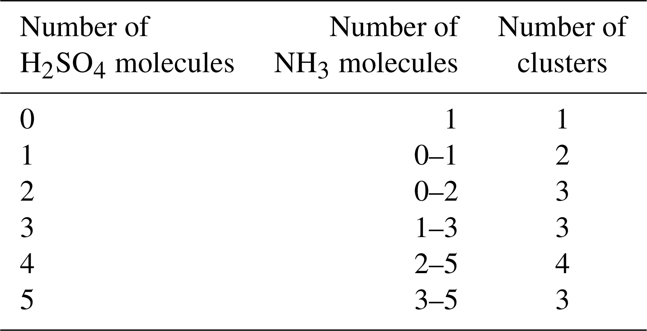
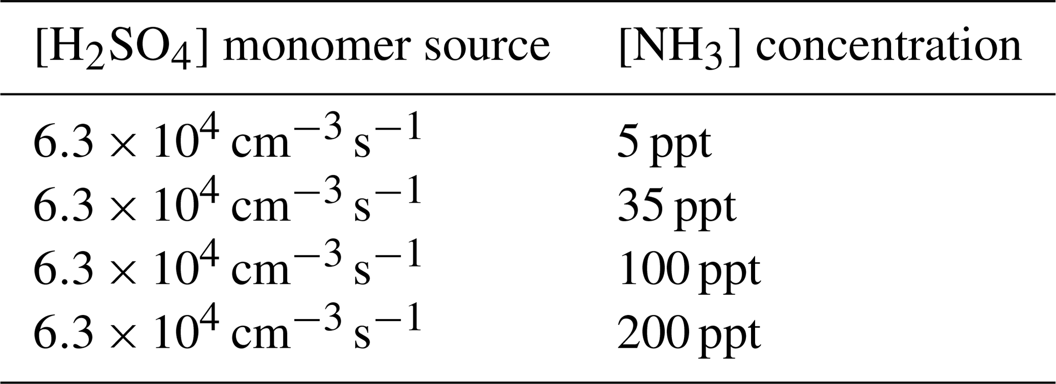
We simulated the time evolution of cluster concentrations using collision rates computed from kinetic gas theory and evaporation rates computed from the Gibbs free energies reported by Olenius et al. (2013b). To save computational time, we omitted clusters where the number of acid and base molecules differed by more than two. Based on both fundamental chemical principles and mass spectrometric data (Kirkby et al., 2011; Schobesberger et al., 2015; Elm and Kristensen, 2017; Yu et al., 2018), these clusters are quite unstable and thus have very high evaporation rates, leading to negligibly low concentrations. See Table 1 for a list of the 16 considered clusters. We included four different ammonia monomer mixing ratios between 5 and 200 ppt, corresponding to concentrations between 1.3×10⁸ and 5.0×10⁹ molecules cm−3 for the temperature ranges studied here. In each individual case, the ammonia mixing ratio was kept constant throughout the simulation. The source rate of sulfuric acid monomer was kept constant at . To reproduce experimental conditions in the CLOUD chamber as closely as possible, the initial sulfuric acid was set to zero in each simulation. See Table 2 for a summary of the concentration settings. Additionally, we considered the losses on the CLOUD chamber walls which depend on the cluster size (Kürten et al., 2015) and a dilution loss of s−1. For simplicity, we omitted the effect of relative humidity. We generated the birth–death equations using the ACDC code (McGrath et al., 2012) and then solved for the cluster concentrations using the Fortran ordinary differential equation solver VODE (Variable-Coefficient ODE Solver) (Brown et al., 1989). These equations and all related parameters are explained in Appendix A1.
Table 1Neutral molecular clusters included in the model system (16 in total). The first column indicates the number of sulfuric acid molecules; the second column indicates the number of ammonia in the cluster.
Our MCMC results are not specific to the set of molecular clusters considered here. This is supported by the fact that although the size of the system (the number of clusters or, more precisely, the maximum size of the clusters included in the simulations) has an impact on the particle formation rates at high temperatures (>278 K), the particle formation rates and cluster concentrations produced using different cluster sets (e.g. 4×4, 5×5 and 6×6 sulfuric acid and ammonia molecules) are qualitatively similar (Besel et al., 2020). Thus, minor changes of the ACDC outputs due to the difference in the sets of considered clusters should not change the MCMC parameter estimation results. Additionally, the boundary conditions for the outgrowing clusters (the choice of the clusters that are considered as formed particles) have only minor influence on the simulation results, as long as the simulated system of clusters is defined in a reasonable way (Besel et al., 2020).
Two data sets were created. In the first set, we generated time-dependent concentrations for each cluster type, measured at 1.5 min time intervals before the system reaches a steady state. This corresponded to a total of 41 time steps. The steady-state single-temperature data correspond to a subset of these data sets. In the second case, we generated steady-state concentrations for all cluster types at two temperatures (278 and 292 K). In both cases, the steady-state cluster concentrations were calculated as the average of the concentrations at t1:=50 min and t2:=60 min. Additionally, we include a convergence parameter for assessing the closeness of cluster concentrations to the steady state for every individual ACDC simulation. This is computed as a ratio of concentrations taken at times t2 and t1. We then selected the ratio which deviated the most from unity, where the maximum was taken over all cluster types (Kupiainen-Määttä, 2016).
Finally, we added measurement error (noise) to the cluster concentrations in both data sets. We call the resulting noisy cluster concentrations “synthetic data”. Our measurement error was sampled from a multivariate Gaussian distribution, with the variance depending on cluster type i, temperature T and time instance t. We assume that the standard deviation of the measurement error is 0.001 % of the original concentration.
2.2 Markov chain Monte Carlo simulations
We used a MCMC-based approach to estimate the evaporation rates which reproduce the synthetic cluster concentration data. Unlike optimization algorithms which compute a single optimal parameter set, MCMC methods sample from a target distribution which contains the most likely combinations of parameter values for the given data. Multiple samples of possible parameter sets are taken along a random walk in the target distribution and are saved as a parameter “chain”. As the length of the chain increases, the sampled sets converge to a probability (posterior) distribution of parameters, which estimates the likelihood of those parameters giving rise to the data. The particular MCMC-based algorithm we use is delayed rejection adaptive Metropolis (DRAM), which is an extended variant of the classical Metropolis algorithm (Metropolis et al., 1953). We chose the DRAM algorithm as it is more efficient than the Metropolis regime at parameter estimation when the parameter space is large (Haario et al., 2006). The two algorithms and their application to our cases are described in the Appendices A2–A3.
2.2.1 Selection of minimum and maximum limits for unknown parameters
We emphasize that there are currently no theoretical principles or experimental results which set sound restrictions for even the order of magnitude of the evaporation rates. However, evaporation rates much lower than 10−10 s−1 are irrelevant in practice, since the timescale for evaporation is then much longer than the cluster lifetime with respect to further growth. Similarly, when the evaporation rate is much greater than 10+10 s−1, the cluster will certainly evaporate before it has a chance to grow further. The base 10 logarithm of the evaporation rates was therefore sampled in the interval of −12 to 12.
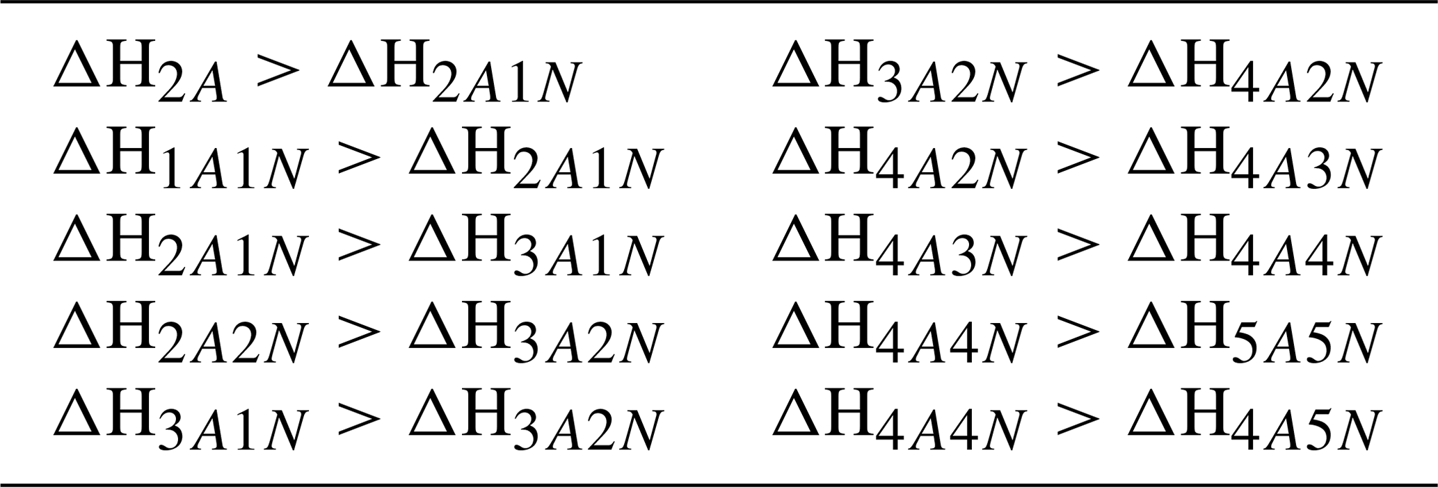
For the cluster formation enthalpies, we chose an upper limit of 0 kcal mol−1, as a positive ΔH would mean an absence of attractive interactions in the molecular cluster, which is physically incorrect for polar, H-bonding molecules such as H2SO4 and NH3. This same argument also applies for each individual molecule, which gives rise to the requirement that the formation enthalpy of each cluster must be lower (more negative) than that of clusters with less acid and/or base molecules. See Table 3 for the full list of restrictions arising from this requirement. As a lower limit for the overall cluster formation enthalpies, we used kcal mol−1. Since our largest clusters contain 10 molecules, this would imply that, on average, each H2SO4 in all the studied clusters is bound substantially stronger than in the exceptionally strongly bound cluster (for which recent high-level computational studies indicate a binding enthalpy roughly around −40 kcal mol−1; Elm et al., 2013; Elm and Kristensen, 2017). This in turn implies that the evaporation rate is zero for all practical purposes.
Table 3Additional restrictions on the cluster formation enthalpies arising from the requirement that each individual molecule is bound The cluster formation enthalpy of the ith cluster is denoted by ΔHi. The notation xAyN corresponds to a cluster with x sulfuric acid and y ammonia molecules.
The upper limit for the formation entropies was set to 0 , as clustering must have a negative formation entropy ΔS, since the number of gas molecules is reduced (and translational and rotational degrees of freedom are thus converted into much more constrained vibrational degrees of freedom). The lower limit of −400 can be justified by noting that the typical per-molecule ΔS for clustering is around −30 , with a typical variation of up to ±10 (Kürten, 2019). For a 10-molecule cluster, this would imply a lower bound to ΔS of around −400 .
2.2.2 Overview of the MCMC runs
We first performed DRAM parameter estimation from both steady-state and time-dependent cluster concentrations at 278 K, treating evaporation rates as the unknown parameters θ. For the time-dependent synthetic data, the number of output coefficients was , where NC=16 is the number of cluster types included into simulations, and Nt=41 is the number of time-step measurements available for each of the cluster types.
Next, we performed parameter estimation based on steady-state cluster concentrations at two temperatures (278 and 292 K). The number of output coefficients in this case was , where NT=2 denotes the number of experiments conducted at different temperatures. We use Eqs. (A4) and (A5) to express the evaporation rates as functions of formation enthalpies, entropies and temperature:
In Eq. (1), we set T=278 K or T=292 K. We emphasize that the rates now depend on temperature and six other parameters: the formation enthalpy ΔHi+j and entropy ΔSi+j of the evaporating/fragmenting cluster i+j and the formation enthalpies ΔHi,ΔHj and entropies ΔSi,ΔSj of the product clusters i and j, respectively. In this setting θ the array of quantities ΔHi+j, ΔSi+j, ΔHi, ΔHj, ΔSi, ΔSj with . Similar approaches were applied for the inverse problem of chemical kinetics modelled by the Arrhenius equation, where chemical reaction rates are temperature dependent (Vahteristo et al., 2008).
Many evaporation/fragmentation reactions have the same clusters as products, and thus several of the pairs ΔHi,ΔSi appear in Eq. (1) for the evaporation rates of multiple different reactant clusters. The formation enthalpies and entropies of monomers are defined in the context of molecular clustering to be zero. The number of distinct unknown formation enthalpies and entropies is thus only 28, compared to 39 unknown evaporation rates. Furthermore, the cluster formation entropy and enthalpy values all lie within 2 orders of magnitude, compared to the evaporation rates which span 24 orders of magnitude. This makes the MCMC method more efficient.
To create a reliable sample from the underlying parameter distribution, the length of the MCMC chain must be “large enough” (Haario et al., 1999, 2001); that is, many different parameter combinations must be tested. In our simulations, the MCMC chain length typically comprised 3 million samples. The MCMC acceptance probabilities (defined below) in each of the cases were about 88.0 %, which is a typical level of acceptance since the forward ACDC model (in which the evaporation and collision rates are known) is deterministic.
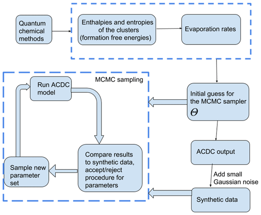
In the MCMC simulations, all sets of parameters which produce cluster concentrations within the allotted noise level of the data (0.001 %) are kept in the chain. The sampling procedure is outlined in Fig. 1. We tested that the MCMC chains converge to the “true” values (Olenius et al., 2013b, i.e. the reference parameter values from) when we start sampling the chain from randomly selected initial guess.
3.1 Identification of evaporation rate coefficients from steady-state data at a single temperature
A graphical representation of the steady-state cluster concentration data at 278 K, as a function of the number of acid molecules in the clusters, is given in Fig. 2.
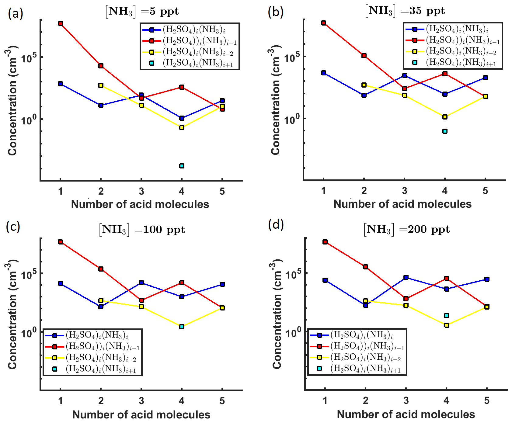
Figure 2Steady-state cluster concentrations for the clusters containing sulfuric acid and a varying number of ammonia molecules, as a function of the number of acid molecules, for [NH3] mixing ratios of (a) 5 ppt, (b) 35 ppt, (c) 100 ppt and (d) 200 ppt at the temperature T=278 K. The concentrations have been amended with multivariate non-correlated Gaussian noise with standard deviation comprising 0.001 % of the original cluster concentration. The source rate of sulfuric acid monomers comprises 6.3×10⁴ s−1.
Next, we determine the base 10 logarithms of the evaporation rate coefficients from the synthetic data. Since the noise added to the cluster concentrations results in a random bias towards an increase (or decrease) from the original values produced from the ACDC, the estimates of parameters derived from synthetic data are likely to be biased. In order to average the effects attributed to this random bias, we generated three sets of synthetic data by adding random increments to the original concentration measurements. Utilizing these data sets, three independent MCMC runs were conducted, each run containing 3 million parameter samples. An example of one of the sampled chains is depicted in Figs. B1 and B2. We omit the initial one million samples and plot the stationary1 parts of the chains. As we observe from the plots in Figs. B1 and B2, all the parameter chains for the evaporation rates have values bounded above by an upper limit, which differs for different evaporation rates. However, only 15 out of 39 evaporation rates are limited from below (see subfigures labelled 1–5, 7, 10, 12, 16, 18, 22, 27, 31, 33 and 35 in Figs. B1 and B2). Notably, all monomer evaporation rates are bounded from below, except for some of the rates from the largest clusters: H2SO4 from (H2SO4)5(NH3)4 and (H2SO4)5(NH3)5, and NH3 from (H2SO4)5(NH3)5.
For each evaporation rate, we calculate the one-dimensional (that is, depending only on the evaporation rate) marginal posterior distribution as the position-wise average of the stationary parts of the three sampled chains. This procedure is needed to average the bias originating from random noise. The resulting distributions are given in Figs. 3 and 4. We use the maximum (also called the mode in the statistics literature) of the posterior marginal distribution function as our parameter estimate in the case when the marginal posterior distributions have precisely one maximum value. In the cases where we have multiple estimators, we provide a range for the evaporation rate values.
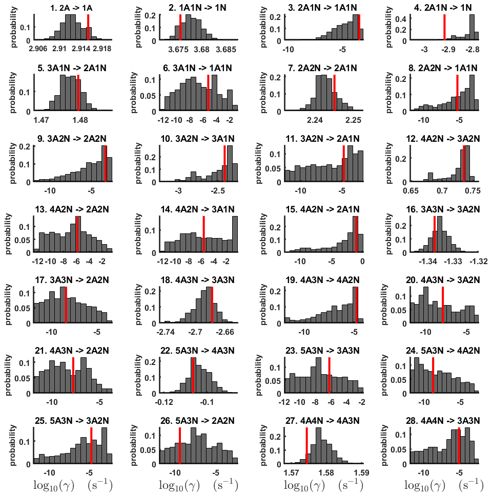
Figure 3One-dimensional marginal posterior distributions (for parameter indexes ranging from 1 to 28) of the base 10 logarithm of the evaporation rates (units given in s−1) determined from steady-state cluster concentration measurements at the temperature 278 K. Red lines denote the baseline values from Olenius et al. (2013b) used to generate the synthetic data. The notation xAyN corresponds to a cluster with x sulfuric acid and y ammonia molecules.
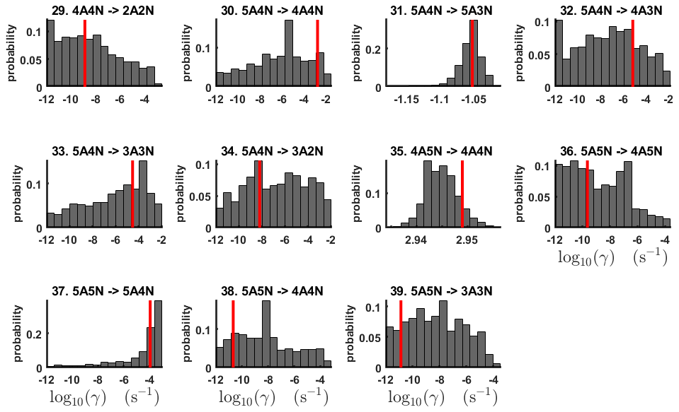
Figure 4One-dimensional marginal posterior distributions (for parameter indexes ranging from 29 to 39) of the base 10 logarithm of the evaporation rates (units given in s−1) determined from steady-state cluster concentration measurements at the temperature 278 K. Red lines denote the baseline values from Olenius et al. (2013b) used to generate the synthetic data. The notation xAyN corresponds to a cluster with x sulfuric acid and y ammonia molecules.
All the evaporation rates larger than 10−3 s−1 are well identified (see subfigures labelled 1, 2, 4, 5, 7, 10, 12, 16, 18, 22, 27, 31 and 35 in Figs. 3 and 4), as their estimated variances are well within our accepted error range of less than 1 order of magnitude. The estimates for the remaining evaporation rates can take values within ranges spanning several orders of magnitude and are thus uncertain. Also, most of the marginal posterior distributions are non-uniform, except for the evaporation rate of (H2SO4)2(NH3)2 from (H2SO4)5(NH3)5. In five cases (refer to subfigures labelled 6, 21, 28, 32 and 36 in Figs. 3 and 4), the estimated parameter values are not unique: the marginal posterior distributions feature multiple modes. The results of our parameter estimation are summarized in Table C1 and in subfigures labelled (a) and (b) in Fig. 5.
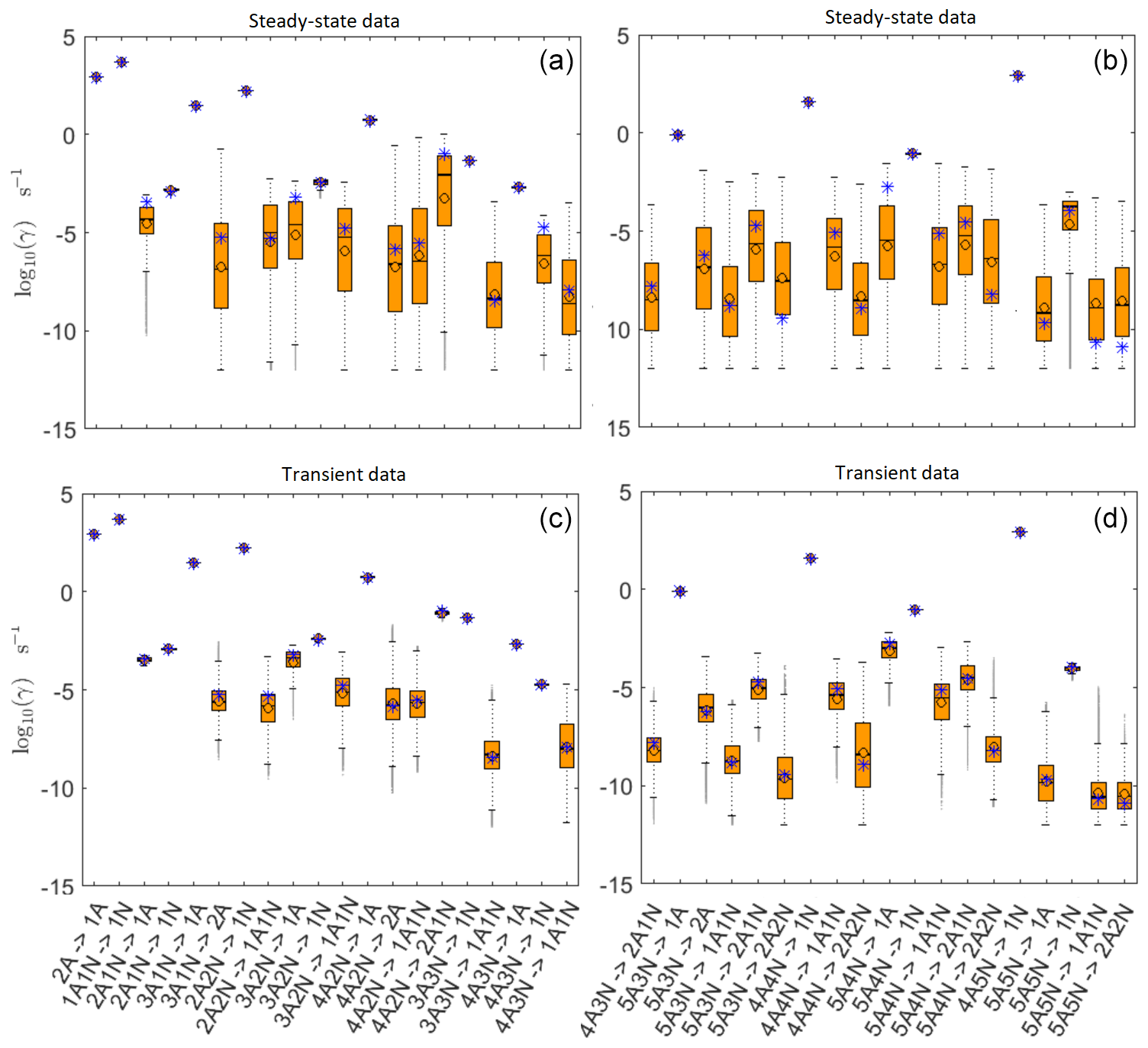
Figure 5Comparison of 95 % confidence intervals (orange box plots) of base 10 logarithms of the evaporation rates determined from (a, b) steady-state and (c, d) time-dependent synthetic data measured at temperature 278 K. Here, blue asterisks denote the baseline values used for creating the synthetic data (borrowed from Olenius et al., 2013b). The black circle and horizontal line markers indicate the mode and the mean value of the distribution, respectively. The notation xAyN corresponds to a cluster with x sulfuric acid and y ammonia molecules.
The pairwise marginal posterior distributions for the estimated evaporation rates are illustrated in Figs. B3–B6. The majority of the parameters are not correlated. However, the evaporation of monomers from (H2SO4)5NH3, (H2SO4)3(NH3)2 and (H2SO4)5(NH3)4 display non-linear inverse correlations. This implies that either H2SO4 rarely evaporates (at a rate less than 10−4 s−1) and that NH3 evaporates often, or that the evaporation rates of H2SO4 and NH3 are of comparable magnitude. Additionally, it can be seen from the pairwise posteriors that most of the estimated parameters are highly uncertain. From a mathematical perspective, the existence of multiple distinct parameter estimates indicates that the problem of recovering evaporation rates from the synthetic steady-state concentration data is ill posed. The general solution to this issue is to regularize the problem either by adding more data or information to the model or by reducing the number of possible estimates.
Based on parameter estimation results, we conclude that a single-temperature steady-state cluster concentrations are not enough to estimate the evaporation rates with a reasonable accuracy (i.e. to obtain an upper and lower limits for the rates that reasonably restrict the cluster kinetics involved in the molecular-level process).
3.2 Identification of evaporation rate coefficients from time-dependent data at a single temperature
The data set for time-dependent cluster concentrations is much larger than the data set for steady-state cluster concentrations, as it contains the concentration values at multiple time instances. The time-dependent data also contain information about the time derivatives of the concentrations (see Fig. C1), which should contribute to quantification of kinetic parameters (in this case evaporation rates). Our time-dependent cluster concentration data sets contain in total 656 concentration measurements (corresponding to 16 cluster types and 41 time steps) for each of the four ammonia mixing ratios.
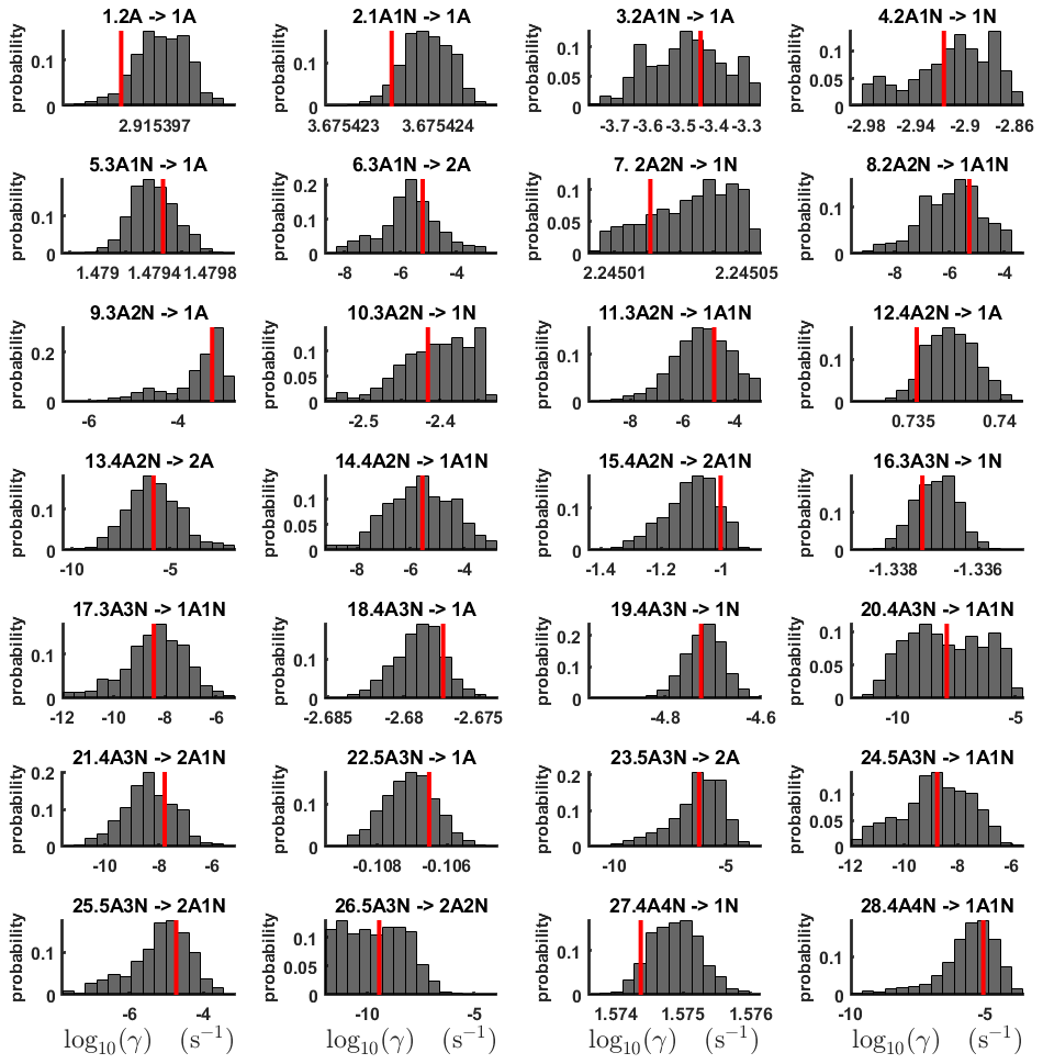
Figure 6One-dimensional marginal posterior distributions (for parameter indexes ranging from 1 to 28) of the base 10 logarithm of the evaporation rates (units given in s−1) determined from time-dependent measurements of the cluster concentrations with time resolution comprising 1.5 min at the temperature 278 K. Red lines denote the baseline values from Olenius et al. (2013b) used to generate the synthetic data. The notation xAyN corresponds to a cluster with x sulfuric acid and y ammonia molecules.
From this time-dependent cluster concentration data set, we then conduct MCMC runs as described in Sect. 2.2. As in the steady-state setting, we conduct three independent MCMC runs to determine the base 10 logarithms of the evaporation rates. One of these runs is presented in Figs. C2 and C3. Again, we omit the first 1 million samples and merge the stationary parts of the sampled chains to obtain the posterior distributions.
As seen in Figs. C2 and C3, all the chains have upper limits. Most of the chains are also bounded from below, with five exceptions. These exceptions, with arbitrarily large magnitudes, are the evaporation rates of (H2SO4)2(NH3)2 from (H2SO4)4(NH3)4 and (H2SO4)5(NH3)3, and the evaporation rates of H2SO4, (H2SO4)(NH3) and (H2SO4)2(NH3)2 from (H2SO4)5(NH3)5.
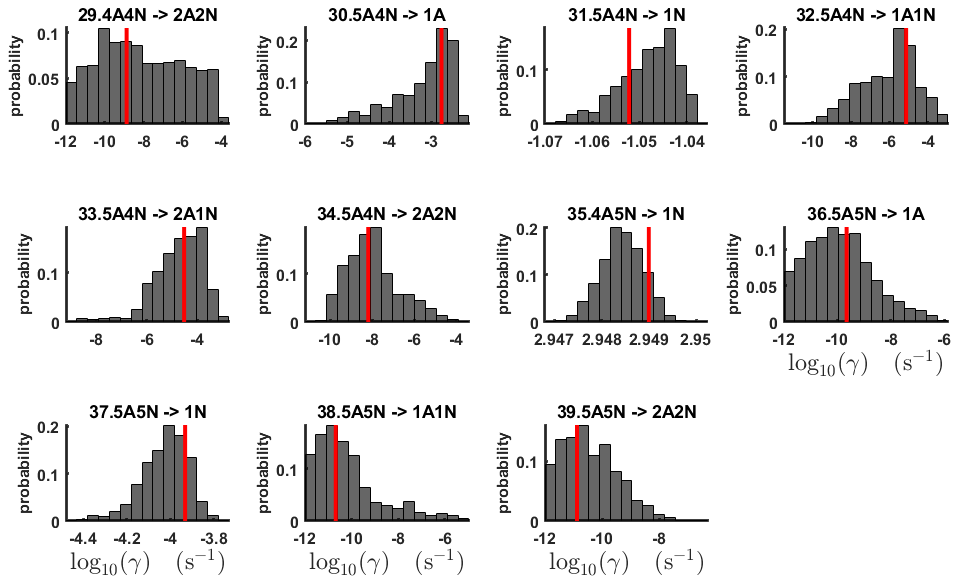
Figure 7One-dimensional marginal posterior distributions (for parameter indexes ranging from 29 to 39) of the base 10 logarithm of the evaporation rates (units given in s−1) determined from time-dependent measurements of the cluster concentrations with time resolution comprising 1.5 min at the temperature 278 K. Red lines denote the baseline values from Olenius et al. (2013b) used to generate the synthetic data. The notation xAyN corresponds to a cluster with x sulfuric acid and y ammonia molecules.
The one-dimensional marginal posterior distributions for the estimated parameters are shown in Figs. 6 and 7. Most of the estimates are close to the “true” values used in the generation of the synthetic data. However, the estimated evaporation rates still feature substantial uncertainties, as their marginal posterior distributions span several orders of magnitude (see subfigures 6, 8, 9, 11, 13, 14, 17, 21, 23–26, 30, 32–34 and 37–39 in Figs. 6 and 7). The evaporation rate of (H2SO4)2(NH3)2 from (H2SO4)5(NH3)3 (which corresponds to subfigure 26) has a uniform posterior distribution, corresponding to an enormous uncertainty. Further, for the evaporation rates depicted in subfigures 20 and 36, we can only determine upper limits of less than s−1. However, the time-dependent data allow us to conclude that the evaporation processes and can be neglected, as they are relatively slow compared with competing evaporation processes.
Pairwise marginal posterior distributions for the evaporation rates are plotted in Figs. C4–C8. Most of the evaporation rates do not display substantial correlations. However, the evaporation rates of monomers from the cluster (H2SO4)2NH3 display a strong inverse linear relationship, indicated by the pairwise marginal posterior distribution of the coefficients and (see Fig. C4). Also, the estimated rate coefficients and exhibit linear correlation. The uncertainties in all the correlated parameters are relatively small (less than an order of magnitude).
In Table C1, we summarize the results of parameter estimation for the two data settings (steady state and time dependent) at a single temperature. Note that the estimated upper limits for some of the small evaporation rates (less than 10−5 s−1) determined from the steady-state data can be as large as s−1. This is a poor estimate, since the uncertainties in the synthetic data are small. For example, see the results for parameters shown in subfigures 32 and 34 of Fig. 7. In these cases, the identification is improved when we extend the data set with time-dependent measurements. Overall, the time-dependent data enabled us to determine the lower bounds for most of the parameters, with the exception of the parameters shown in subfigures numbered 26 and 29. Moreover, the additional time-dependent data enabled us to reduce the uncertainties in the estimates of parameters in subfigures 15, 19 and 37. As a result, with the aid of time-dependent data we have improved the estimates of minimal and maximal values for the evaporation rate parameters (see the comparison of the 95 % confidence intervals plotted in Fig. 5).
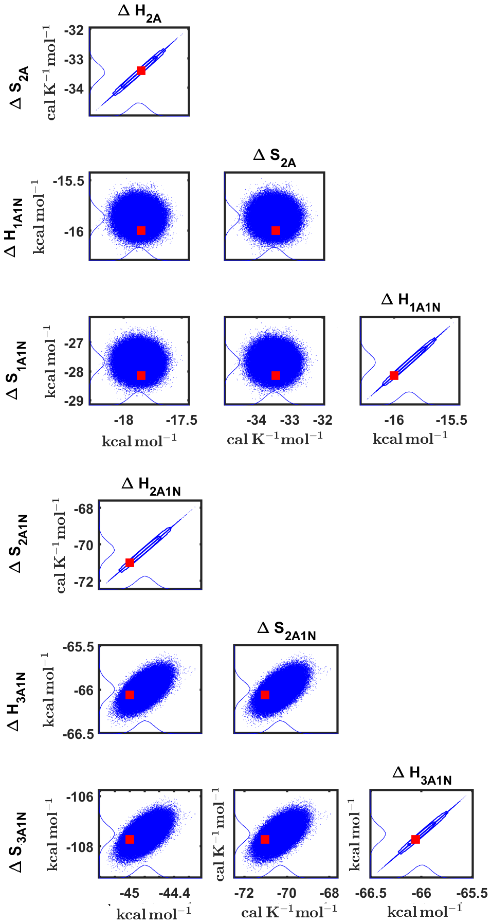
Figure 8Pairwise marginal posterior distributions (for parameter indexes ranging from 1 to 8) of the cluster formation enthalpies and entropies determined from steady-state cluster concentration measurements at two temperatures (T=278 K and T=292 K). Red rectangles denote the baseline values from Olenius et al. (2013b) used to generate the synthetic data. Here, the symbols ΔH and ΔS stand for cluster formation enthalpies and entropies, respectively. The notation xAyN corresponds to a cluster with x sulfuric acid and y ammonia molecules.
3.3 Estimating formation enthalpies and entropies from steady-state concentration measurements at multiple temperatures
We determined cluster formation enthalpies and entropies based on two sets of steady-state cluster concentrations, corresponding to two temperatures: 278 and 292 K. These data sets are plotted in Figs. 2 and D1 for 278 and 292 K, respectively. As in the previous sections, three MCMC runs were conducted to average the bias attributed to random noise. An example of the sampled chains is shown in Fig. D2. It can be seen that all the chains are bounded, with the exception of the formation enthalpy and entropy of the largest cluster ).
The one-dimensional marginal posterior distributions of the formation enthalpies and entropies, built from the stationary parts of the three sampled chains merged together, are shown in Fig. 9. For all the clusters except (H2SO4)5(NH3)5, the variances of the estimated formation enthalpies are less than 0.46 kcal mol−1, while the estimated formation entropies vary at most by 5.4 . The estimated free parameters together with the “true” quantum-chemistry-based values from Olenius et al. (2013b) used for generation of the synthetic data are summarized in Table D1.
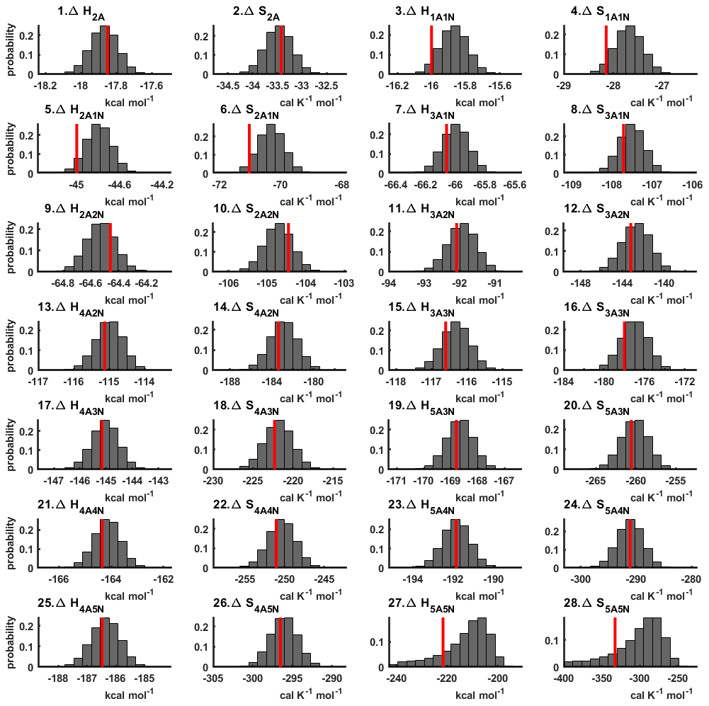
Figure 9One-dimensional marginal posterior distributions of the cluster formation enthalpies (units given in kcal mol−1) and entropies (units given in ) determined from steady-state cluster concentration measurements at two temperatures (T=278 K and T=292 K). Red lines denote the baseline values from Olenius et al. (2013b) used to generate the synthetic data. Here, the symbols ΔH and ΔS stand for cluster formation enthalpies and entropies, respectively. The notation xAyN corresponds to a cluster with x sulfuric acid and y ammonia molecules.
Although the posterior distributions of the formation enthalpies and entropies of (H2SO4)5(NH3)5 feature higher uncertainties in comparison to those of the smaller clusters, the evaporation rates from (H2SO4)5(NH3)5, as calculated from the aforementioned posterior distributions, have low variances; see Table D2. Additionally, strong correlations are observed between formation enthalpies and entropies of clusters containing the same number n of ammonia molecules when n>2, except the case of (H2SO4)5(NH3)5 (see Fig. 8). These strong correlations are consistent with general principles of clustering thermodynamics. If a cluster has very strong bonds between its constituent molecules, then the formation enthalpy is very negative, and also the intermolecular vibrational frequencies corresponding in a broad sense to vibrations involving those bonds are fairly high, meaning that the entropy loss in forming the cluster is large. These intermolecular frequencies dominate the “variable part” of the formation entropy, as the entropy change from the loss of translational and rotational degrees of freedom is almost a constant factor. Thus, if the formation enthalpy of a cluster is very negative, so is also the formation entropy. Conversely, if the cluster is only quite weakly bound, the formation enthalpy is only slightly negative, and the intermolecular frequencies can be very low, leading to a less negative (though still negative) formation entropy. Evaporation rates for all the molecular clusters calculated from a posterior distribution of sampled formation enthalpies and entropies are close to the “true” values used for generation of the synthetic data at both temperatures (278 and 292 K) and their variances are less than 1 order of magnitude; see Figs. D6 and D7. Thus, reparameterization of evaporation rates in terms of formation enthalpies and entropies, and use of data at two different temperatures, transforms our parameter estimation problem from an ill-posed to a well-posed one.
We applied Bayesian parameter estimation using a Markov chain Monte Carlo (MCMC) algorithm to identify cluster evaporation/fragmentation rates from synthetic cluster distribution data, assuming that the cluster collision rates are known. We used the Atmospheric Cluster Dynamics Code (ACDC) together with evaporation rates based on quantum chemistry and detailed balance to generate synthetic data for the purpose of optimizing and validating the parameter estimation.
First, we sought to determine the cluster evaporation rates from both steady-state and time-dependent cluster concentration data at one temperature. We were only able to identify a subset of the free parameters (evaporation rates) from the available data using either of these approaches.
Next, we used steady-state concentration data corresponding to two different temperatures. We introduced a reparameterization which expressed the evaporation rates in terms of temperature and cluster formation enthalpies and entropies. Using steady-state concentrations at two temperatures allowed us to apply two general principles of inverse problems/Bayesian estimation to the problem of estimating evaporation rates. First, the two-temperature data set enabled us to reformulate the problem in a numerically effective way (in terms of formation enthalpies and entropies), which reduced the number of unknown parameters. This reduced the number of parameters we sought to identify. Second, it also lessened the stiffness of the system, as the cluster formation enthalpies and entropies for our system span a much smaller range compared to the evaporation rates. We demonstrated that steady-state concentration data at two different temperatures could be used to determine all the unknown formation enthalpies and entropies, and thus the evaporation rates, to within acceptable accuracy. In practice, the most important evaporation rates for modelling new particle formation are those which are roughly of the same order of magnitude as the rates at which the clusters collide with the vapour molecules. If we assume that the mixing ratios for the clustering vapours are in the ppt–ppb range and use kinetic gas theory collision rates for small molecules and nanometre-sized clusters, we approximately should obtain evaporation rates in the range of 10−3 to 103 s−1. Fortunately, our approach is able to constrain these evaporations rates to within a factor of 10 or less. Evaporation rates below 10−4 s−1 are not as well constrained. However, the corresponding processes are usually not relevant for determining overall new particle formation rates. While the high accuracy of estimated evaporation rates originates from the assumptions of small-noise synthetic data and the concentrations measured for all the cluster types, similar accuracy can be expected if high-quality experimental steady-state data at two temperatures are used instead.
In general, the accuracy of the MCMC results naturally increases when we include additional data. In particular, including more concentration data measured at different ammonia concentrations will yield better estimates for the evaporation rates. The sensitivity of the estimates to the number of ammonia concentrations, as well as different sulfuric acid source rates, will be considered in future work.
The approach presented here can also be applied to infer evaporation rates from mass spectrometric measurements of molecular cluster concentrations. This naturally requires accounting for the process of charging neutral clusters, with its associated instrumental and data-analysis-related uncertainties. A clear conclusion of our proof-of-concept study is that steady-state data at different temperatures are more useful for determining evaporation rates than time-dependent data at a single temperature. Moreover, reliable steady-state concentrations of clusters at various temperatures are generally easier to obtain experimentally (e.g. in chamber experiments) compared to time-dependent concentrations. This finding demonstrates the more general feature of modelling of the type performed here: it can be used to optimize planning of experiments and thus save both time and resources. Determining very low (below 10−5 s−1) evaporation rates may also require additional measurements at low vapour concentrations, which naturally require longer timescales to reach a steady state. Treating the uncertainties inherent in experimental data will be the topic of our future studies.
A1 Cluster kinetics
The kinetics of cluster formation are described by Becker–Döring equations (Ball et al., 1986; Hingant and Yvinec, 2017), which model cluster birth and death which arise from collisions of the smaller clusters into larger ones and evaporations from the bigger clusters into smaller ones. Precisely, labelling the clusters by , the time derivative of the ith cluster concentration Yi is governed by
where βi,j is the collision coefficient of clusters i with j, and is the evaporation coefficient of cluster i+j into clusters i and j, Qi is an external source term of i, and Si represents the total possible types of losses for the cluster of type i. These last two terms, which stand for external supply and destruction mechanisms, depend on the system under consideration.
We now specify the quantity and type of sinks and sources included in our studies. We assume that the concentration of ammonia monomers is constant, while sulfuric acid monomers are supplied to the system at a constant rate comprising . This settings are selected to imitate the conditions inside of the CLOUD chamber (Kirkby et al., 2011; Kürten et al., 2015). Further, we include wall losses arising from clusters sticking on the walls of the experimental chamber (Kürten et al., 2015). These wall losses are parameterized by the size of the cluster
where ri is the mass radius of the cluster (in cm). From Eq. (A2), wall loss rates decrease with cluster size; in practise, it also varies with respect to cluster position in the chamber and time. We neglect any uncertainties attributed to the wall losses. However, we do account for dilution losses, with size-independent value comprising s−1, which had previously been determined in the CLOUD chamber (Kirkby et al., 2011; Kürten et al., 2015).
Let T denote the temperature of the system of molecular clusters. Using classical kinetic gas theory, the collision rates βi,j in Eq. (A1) obey
where mi and Vi are, respectively, the mass and volume of cluster i, and kB is Boltzmann's constant. In this paper, we assume that the masses and volumes are temperature independent.
The cluster evaporation rates in Eq. (A1) are given by the expression
where Pref is the reference pressure and ΔGi is the Gibbs free energy of formation for cluster i. We may further describe the ith Gibbs free energy in terms of the cluster formation enthalpy ΔHi and entropy ΔSi:
We neglect here the weak temperature dependence of real cluster formation enthalpies and entropies.
A2 The Metropolis algorithm
We first select the flat prior distribution from which we will initially sample unknown parameters, as we wish to generate physically reasonable parameter estimates. Therefore, we generate unknown parameters within the chosen minimum and maximum bounds where all the points are equally likely to be sampled. Please see Sect. 2.2.3 and Tables 3 and 4 for more details. From the prior distribution, a starting guess for the parameters is chosen (here ncoef is the total number of parameters).
The Metropolis algorithm then requires us to specify how to sample new parameter values θnew. This is done by choosing a proposal distribution. We chose a multivariate Gaussian proposal density q, defined by
where Σ is a covariance matrix (of dimensions ncoefs×ncoefs) which specifies the scaling and spatial orientation of the Gaussian proposal distribution. As the normalization constants are cancelled out in Eq. (A9), we do not take them into consideration.
Next, we run the ACDC and Fortran simulations with the parameter values θnew. We collect the cluster concentration outputs in the column vector , where nout is the number of elements. The candidate vector of parameters θnew is either accepted or rejected according to the least-square fit of ymod(θnew) to the synthetic cluster concentrations yexp:
where nout is the number of measurements in the synthetic concentrations. By construction, our synthetic data contain uncorrelated Gaussian measurement error; hence, the likelihood of observing the data yexp given some parameter values θ is
The value SS(θnew) is then compared to the least-square sum from the previous step SS(θold) and accepted with the probability
If θnew is accepted, this parameter combination is added as the next element in the chain; otherwise, the old value is replicated in the chain. Finally, the value SS(θold) is replaced with SS(θnew) and saved. This completes an iteration of the Metropolis algorithm.
We remark here that the likelihoods p(yexp|θold) and p(yexp|θnew) in Eq. (A9) characterize how closely the outputs of the ACDC simulations with the parameters θold and θnew, respectively, fit the synthetic data. By definition of the acceptance probability pacc(θold,θnew) in Eq. (A9), the candidate step is always accepted if the new parameters fit the data at least as well as the old values (SS(θnew)≤SS(θold)).
A3 The DRAM algorithm for sampling from large parameter space
Our implementation of the DRAM (Mira, 2001; Haario et al., 2001) approach to MCMC parameter estimation modifies the above Metropolis algorithm in the following way.
First, we use the adaptive Metropolis (AM) (Haario et al., 2001) method for updating the covariance matrix Σ of the proposal distribution q(θold,θnew) in Eq. (A6). That is, if we have generated samples , the next candidate set θnew is proposed from using the empirical covariance . Therefore, the next candidate set is generated by taking a step with direction and size determined from the values of parameters previously sampled in the MCMC chain. This procedure is carried out after every 100 successive accept/reject iterations. To ensure computational stability, we also apply additional scaling and regularization for the proposal covariance (see Gelman et al., 2004; Haario et al., 2001); please see Haario et al. (2006) for a detailed explanation.
Second, we carry out local adaptation of the proposal distribution using the delayed rejection (DR) algorithm (Mira, 2001). It is implemented as follows: given n parameter sets generated by the AM method above, a candidate θnew is proposed from the distribution q(θn,θnew) in Eq. (A6) and accepted with probability as in Eq. (A9), as discussed before. However, if the proposed θnew is rejected, instead of replicating the previous values in the MCMC chain (i.e. ), the algorithm tests a new candidate move θnew,2 which is close to the current estimate θn. Then, the second-stage proposal θnew,2 is accepted with appropriately adjusted acceptance probability (see Haario et al., 2006).
In summary, our application of the DRAM algorithm combines the AM procedure with a two-stage DR modification. In the first stage, our algorithm carries out the Metropolis regime with both AM adaptation. The proposal covariance at the initialization of DR (denoted as Σ) is computed as by AM method above, no matter at which stage of DR these points have been accepted in the sampling process. The covariance of the proposal for the second stage (denoted as Σ2) is always computed as the scaled version of the first-stage proposal covariance:
with the scaling coefficient that was chosen to increase the number of accepted candidate steps at the second stage (Haario et al., 2006).
This DRAM parameter estimation was conducted using the mcmcstat toolbox implemented for FORTRAN (Haario et al., 2001, 2006). See the description and the examples of usage at https://mjlaine.github.io/mcmcf90/ (last access: 9 December 2020).
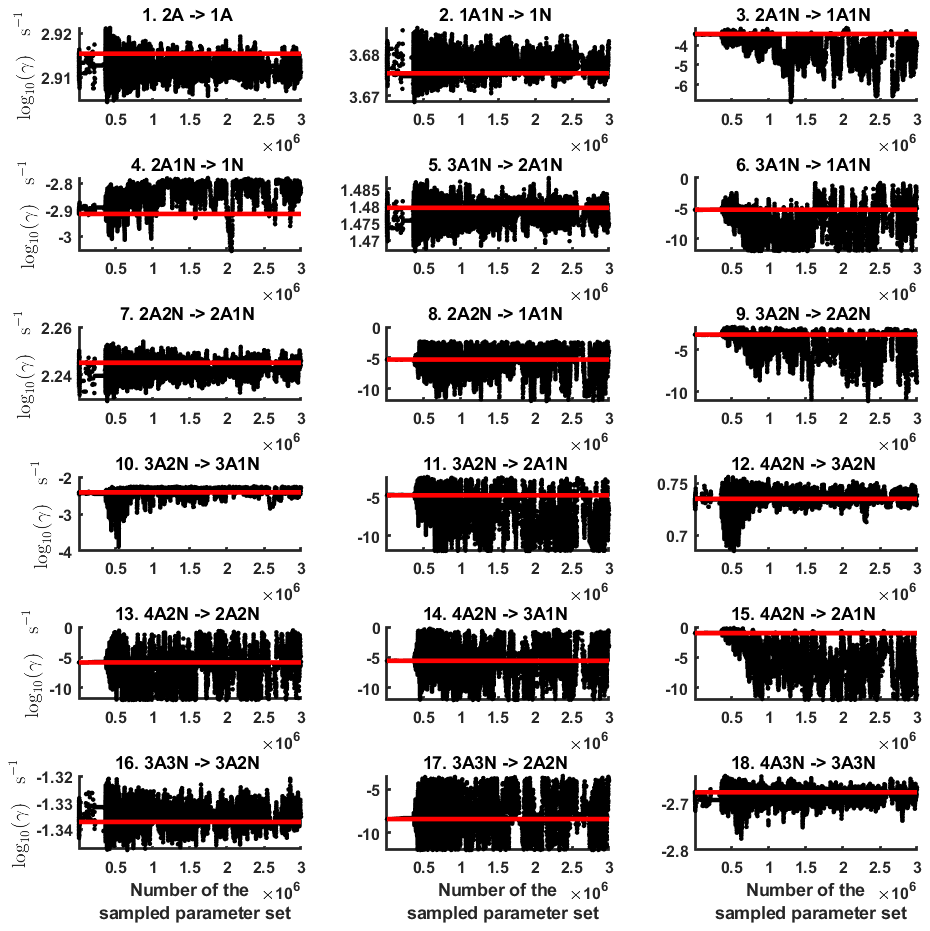
Figure B1Parameter chains (for parameter indexes ranging from 1 to 18) of the base 10 logarithm of the evaporation rates (units given in s−1) determined from steady-state cluster concentration measurements at the temperature 278 K. Red lines denote the baseline values from Olenius et al. (2013b) used to generate the synthetic data. The notation xAyN corresponds to a cluster with x sulfuric acid and y ammonia molecules.
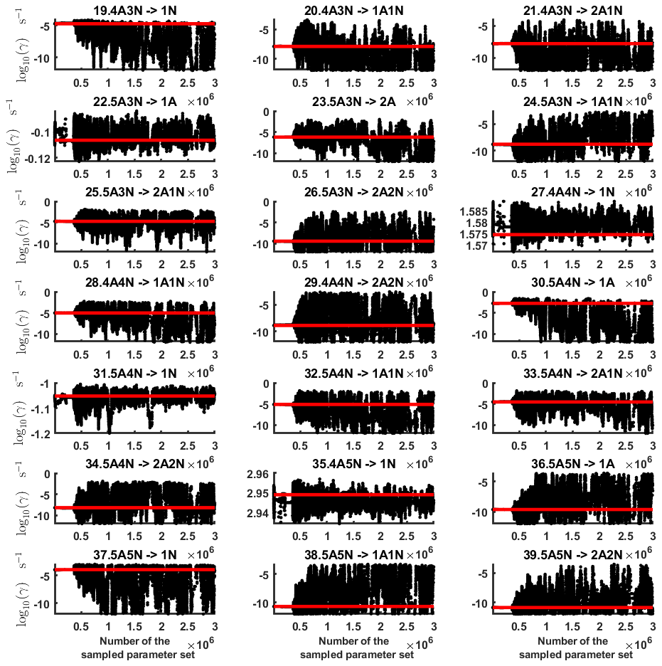
Figure B2Parameter chains (for parameter indexes ranging from 19 to 39) of the base 10 logarithm of the evaporation rates (units given in s−1) determined from steady-state cluster concentration measurements at the temperature 278 K. Red lines denote the baseline values from Olenius et al. (2013b) used to generate the synthetic data. The notation xAyN corresponds to a cluster with x sulfuric acid and y ammonia molecules.
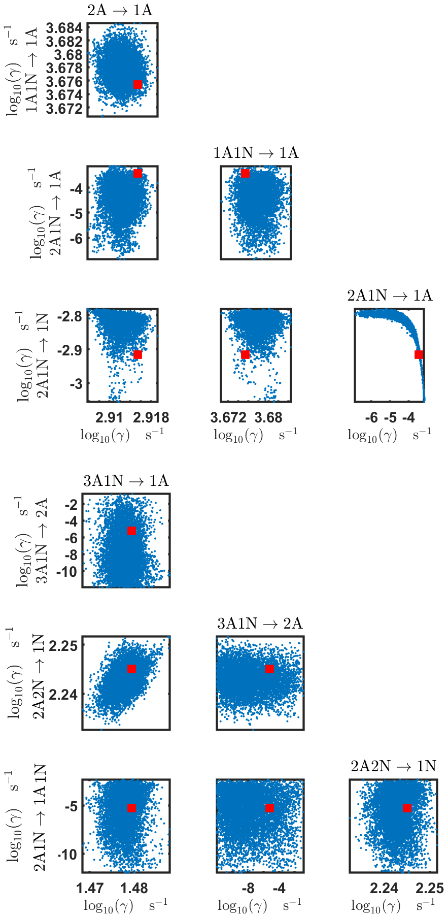
Figure B3Pairwise marginal posterior distributions (for parameter indexes ranging from 1 to 8) of the base 10 logarithm of the evaporation rates (units given in s−1) determined from steady-state cluster concentration measurements at the temperature 278 K. Red rectangles denote the baseline values from Olenius et al. (2013b) used to generate the synthetic data. The notation xAyN corresponds to a cluster with x sulfuric acid and y ammonia molecules.
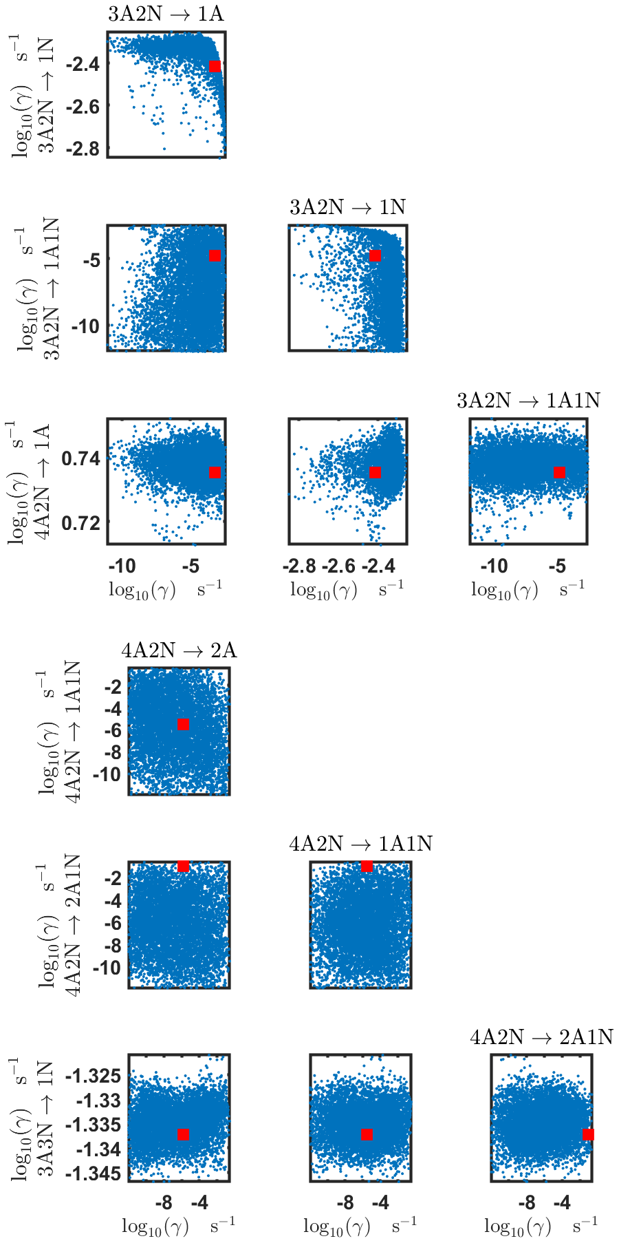
Figure B4Pairwise marginal posterior distributions (for parameter indexes ranging from 9 to 16) of the base 10 logarithm of the evaporation rates (units given in s−1) determined from steady-state cluster concentration measurements at the temperature 278 K. Red rectangles denote the baseline values from Olenius et al. (2013b) used to generate the synthetic data. The notation xAyN corresponds to a cluster with x sulfuric acid and y ammonia molecules.
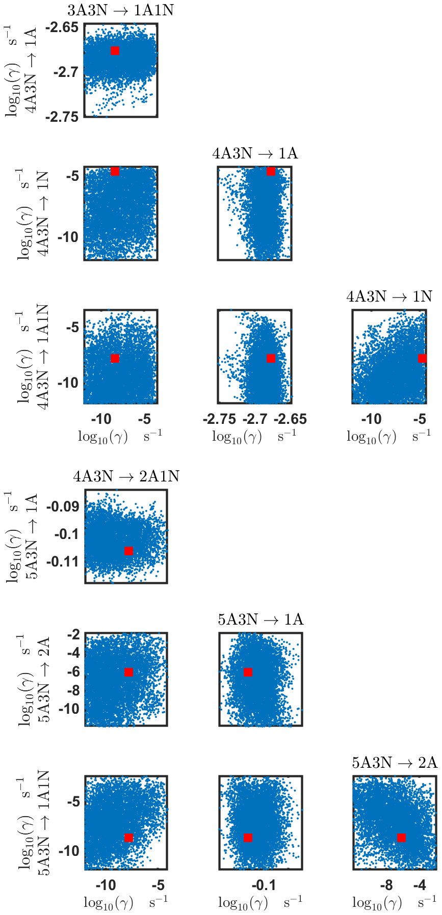
Figure B5Pairwise marginal posterior distributions (for parameter indexes ranging from 17 to 24) of the base 10 logarithm of the evaporation rates (units given in s−1) determined from steady-state cluster concentration measurements at the temperature 278 K. Red rectangles denote the baseline values from Olenius et al. (2013b) used to generate the synthetic data. The notation xAyN corresponds to a cluster with x sulfuric acid and y ammonia molecules.
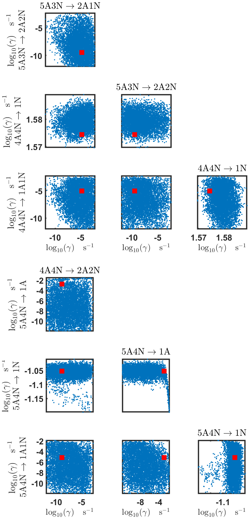
Figure B6Pairwise marginal posterior distributions (for parameter indexes ranging from 25 to 32) of the base 10 logarithm of the evaporation rates (units given in s−1) determined from steady-state cluster concentration measurements at the temperature 278 K. Red rectangles denote the baseline values from Olenius et al. (2013b) used to generate the synthetic data. The notation xAyN corresponds to a cluster with x sulfuric acid and y ammonia molecules.
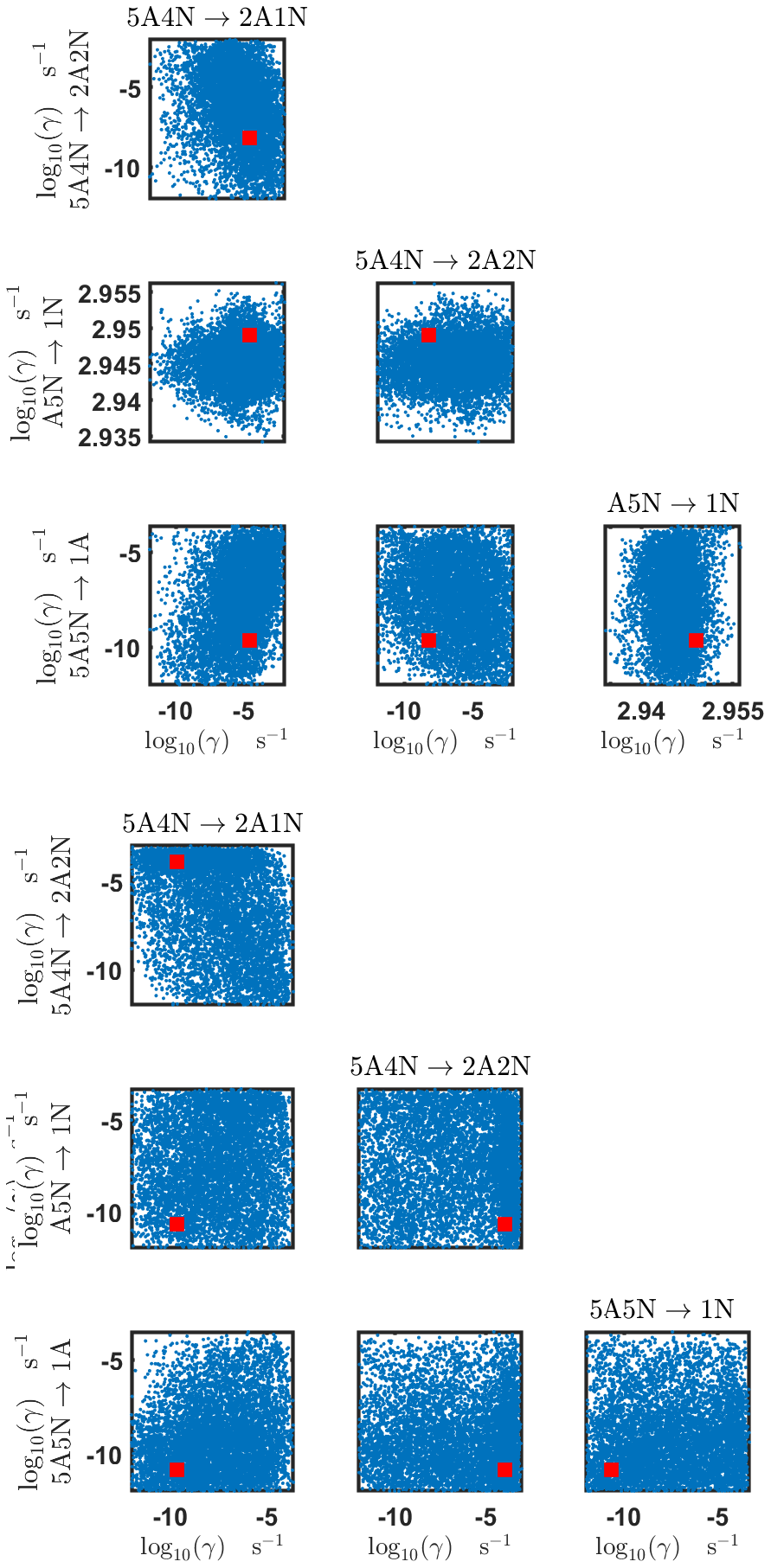
Figure B7Pairwise marginal posterior distributions (for parameter indexes ranging from 33 to 39) of the base 10 logarithm of the evaporation rates (units given in s−1) determined from steady-state cluster concentration measurements at the temperature 278 K. Red rectangles denote the baseline values from Olenius et al. (2013b) used to generate the synthetic data. The notation xAyN corresponds to a cluster with x sulfuric acid and y ammonia molecules.

Figure C1Time-dependent cluster concentrations. Simulated time evolution of concentrations for different cluster types at temperature T=278 K for varying [NH3] concentration: 5, 35, 100 and 200 ppt (see the legend). All the model outputs are amended with multivariate non-correlated Gaussian noise with standard deviation comprising 0.001% of the original cluster concentration. Time resolution comprises 1.5 min. The source of sulfuric acid monomer is s−1 in all simulations. The notation xAyN corresponds to a cluster with x sulfuric acid and y ammonia molecules.
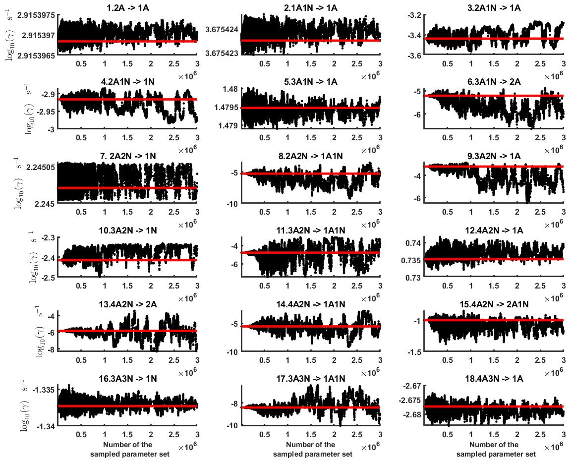
Figure C2Parameter chains (for parameter indexes ranging from 1 to 28) of the base 10 logarithm of the evaporation rates (units given in s−1) determined from time-dependent measurements of the cluster concentrations with time resolution comprising 1.5 min at the temperature 278 K. Red lines denote the baseline values from Olenius et al. (2013b) used to generate the synthetic data. The notation xAyN corresponds to a cluster with x sulfuric acid and y ammonia molecules.
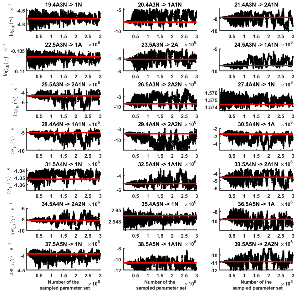
Figure C3Parameter chains (for parameter indexes ranging from 29 to 39) of the base 10 logarithm of the evaporation rates (units given in s−1) determined from time-dependent measurements of the cluster concentrations with time resolution comprising 1.5 min at the temperature 278 K. Red lines denote the baseline values from Olenius et al. (2013b) used to generate the synthetic data. The notation xAyN corresponds to a cluster with x sulfuric acid and y ammonia molecules.
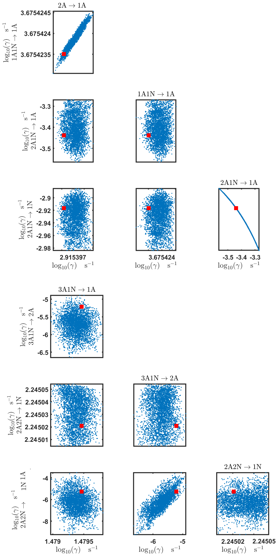
Figure C4Pairwise marginal posterior distributions (for parameter indexes ranging from 1 to 8) of the base 10 logarithm of the evaporation rates (units given in s−1) determined from time-dependent measurements of the cluster concentrations with time resolution comprising 1.5 min at the temperature 278 K. Red rectangles denote the baseline values from Olenius et al. (2013b) used to generate the synthetic data. The notation xAyN corresponds to a cluster with x sulfuric acid and y ammonia molecules.

Figure C5Pairwise marginal posterior distributions (for parameter indexes ranging from 9 to 16) of the base 10 logarithm of the evaporation rates (units given in s−1) determined from time-dependent measurements of the cluster concentrations with time resolution comprising 1.5 min at the temperature 278 K. Red rectangles denote the baseline values from Olenius et al. (2013b) used to generate the synthetic data. The notation xAyN corresponds to a cluster with x sulfuric acid and y ammonia molecules.
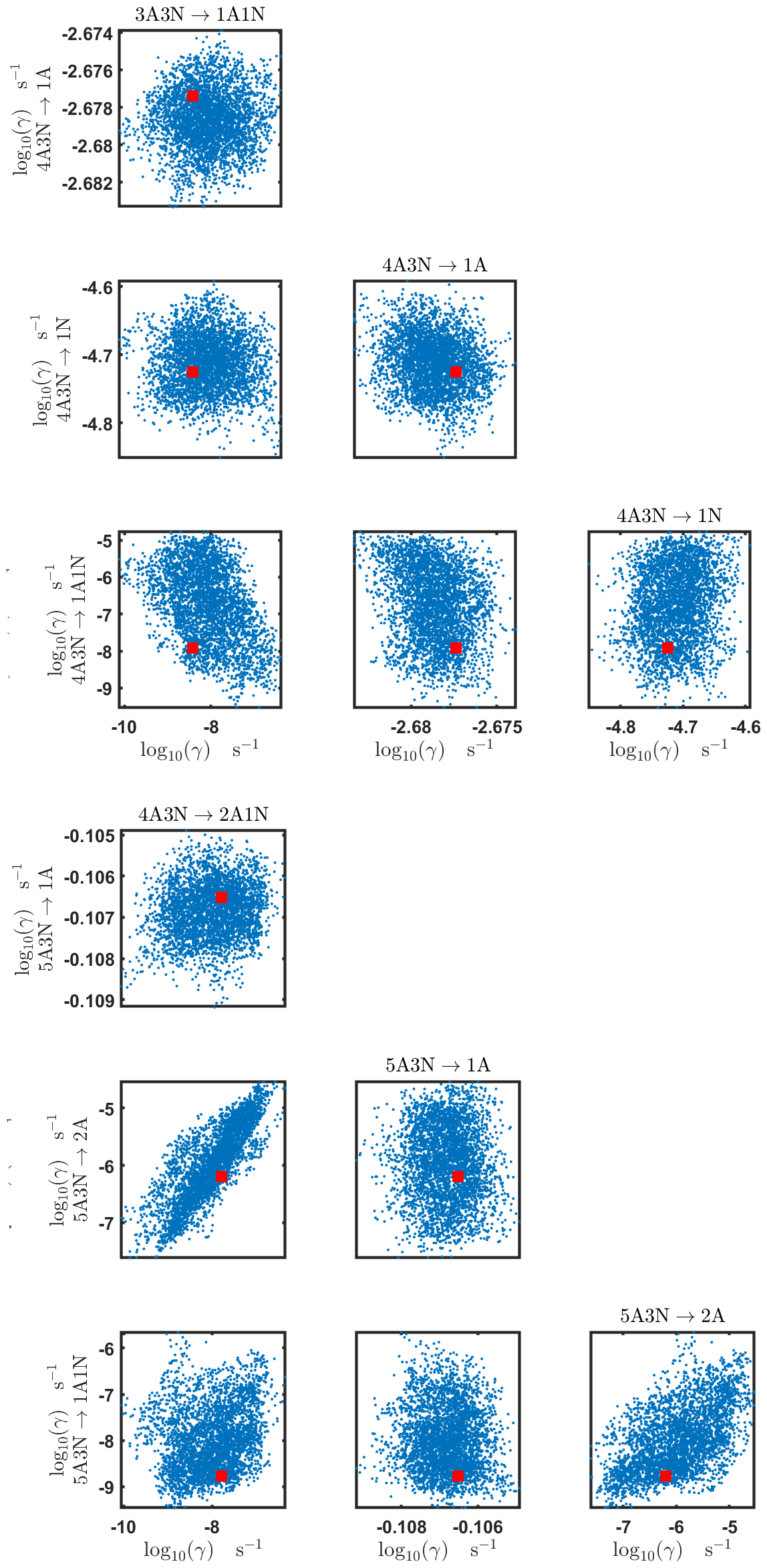
Figure C6Pairwise marginal posterior distributions (for parameter indexes ranging from 17 to 24) of the base 10 logarithm of the evaporation rates (units given in s−1) from time-dependent measurements of the cluster concentrations with time resolution comprising 1.5 min at the temperature 278 K. Red rectangles denote the baseline values from Olenius et al. (2013b) used to generate the synthetic data. The notation xAyN corresponds to a cluster with x sulfuric acid and y ammonia molecules.
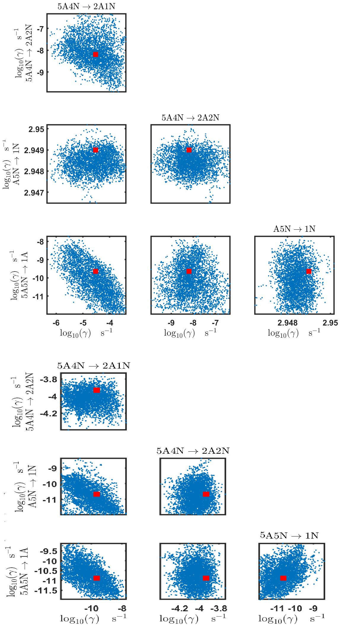
Figure C7Pairwise marginal posterior distributions (for parameter indexes ranging from 25 to 32) of the base 10 logarithm of the evaporation rates (units given in s−1) from time-dependent measurements of the cluster concentrations with time resolution comprising 1.5 min at the temperature 278 K. Red rectangles denote the baseline values from Olenius et al. (2013b) used to generate the synthetic data. The notation xAyN corresponds to a cluster with x sulfuric acid and y ammonia molecules.
Table C1Evaporation rates (units given in s−1) determined from the steady-state and the time-dependent data presented in Figs. 5, 6, 16 and 17, respectively. For parameters that have a posterior distribution with the clear peak and practically zero probability density elsewhere, the mode of the distribution (in bold) is given together with the range of possible values in the parentheses. In some of the cases, only the limits can be determined. The last column presents the baseline values from Olenius et al. (2013b) used to generate the synthetic data. The notation xAyN corresponds to a cluster with x sulfuric acid and y ammonia molecules.
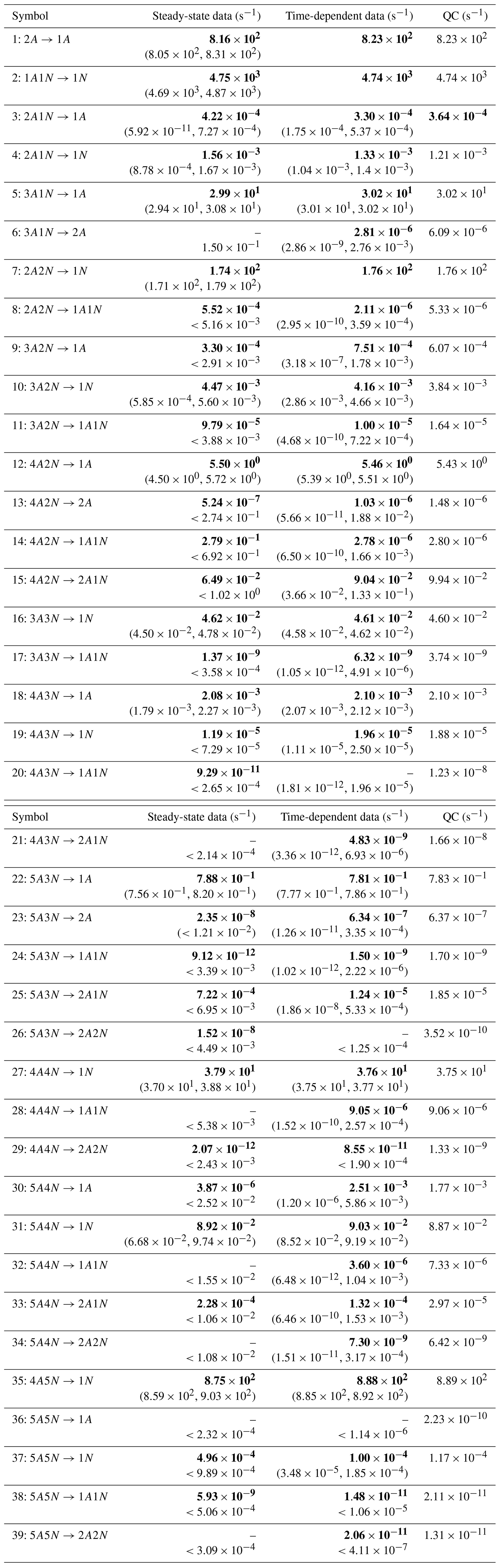
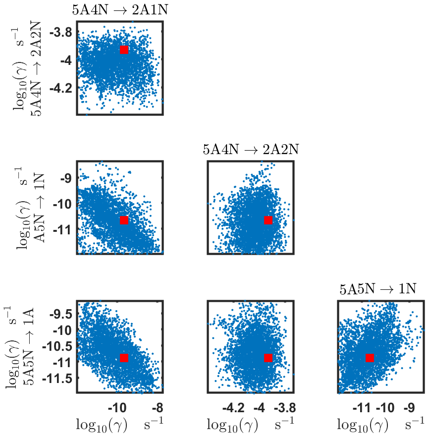
Figure C8Pairwise marginal posterior distributions (for parameter indexes ranging from 33 to 39) of the base 10 logarithm of the evaporation rates (units given in s−1) from time-dependent measurements of the cluster concentrations with time resolution comprising 1.5 min at the temperature 278 K. Red rectangles denote the baseline values from Olenius et al. (2013b) used to generate the synthetic data. The notation xAyN corresponds to a cluster with x sulfuric acid and y ammonia molecules.

Figure D1Steady-state cluster concentrations for the clusters containing sulfuric acid and a varying number of ammonia molecules as a function of the number of acid molecules for [NH3] concentrations comprising (a) 5 ppt, (b) 35 ppt, (c) 100 ppt and (d) 200 ppt at temperature T=292 K amended with multivariate non-correlated Gaussian noise with standard deviation comprising 0.001% of the original cluster concentration. The source of sulfuric acid monomer comprises 6.3×10⁴ s−1 in all the simulations. Here, the symbols ΔH and ΔS stand for cluster formation enthalpies and entropies, respectively. The notation xAyN corresponds to a cluster with x sulfuric acid and y ammonia molecules.
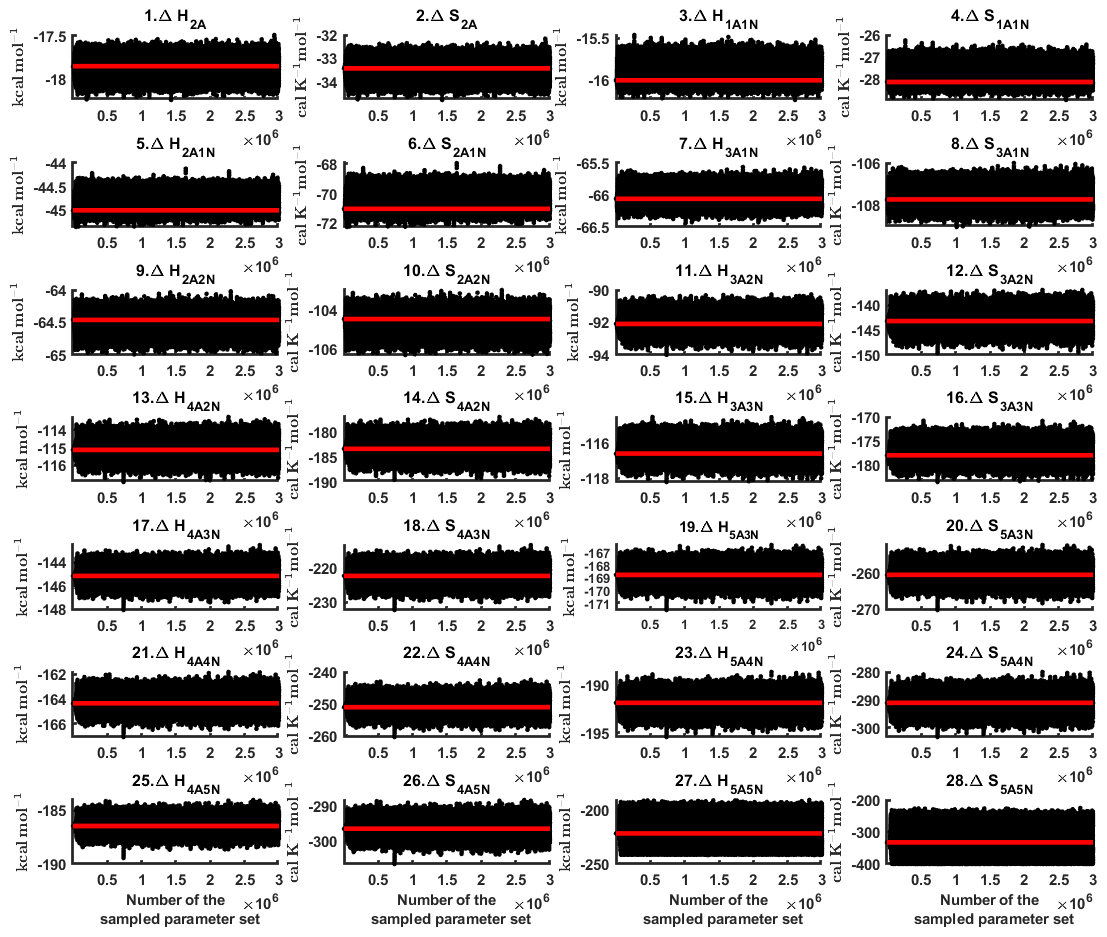
Figure D2Parameter chains of the cluster formation enthalpies (units given in kcal mol−1) and entropies (units given in ) determined from steady-state cluster concentration measurements at two temperatures (T=278 K and T=292 K). Red lines denote the baseline values from Olenius et al. (2013b) used to generate the synthetic data. Here, the symbols ΔH and ΔS stand for cluster formation enthalpies and entropies, respectively. The notation xAyN corresponds to a cluster with x sulfuric acid and y ammonia molecules.
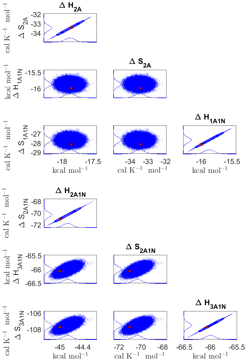
Figure D3Pairwise marginal posterior distributions (for parameter indexes ranging from 9 to 16) of the cluster formation enthalpies and entropies determined from steady-state cluster concentration measurements at two temperatures (T=278 K and T=292 K). Red rectangles denote the baseline values from Olenius et al. (2013b) used to generate the synthetic data. Here, the symbols ΔH and ΔS stand for cluster formation enthalpies and entropies, respectively. The notation xAyN corresponds to a cluster with x sulfuric acid and y ammonia molecules.
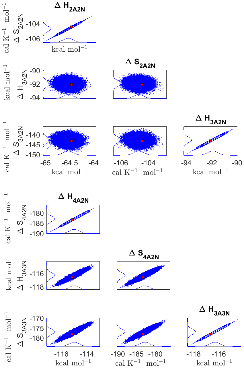
Figure D4Pairwise marginal posterior distributions (for parameter indexes ranging from 17 to 24) of the cluster formation enthalpies and entropies determined from steady-state cluster concentration measurements at two temperatures (T=278 K and T=292 K). Red rectangles denote the baseline values from Olenius et al. (2013b) used to generate the synthetic data. Here, the symbols ΔH and ΔS stand for cluster formation enthalpies and entropies, respectively. The notation xAyN corresponds to a cluster with x sulfuric acid and y ammonia molecules.

Figure D5Pairwise marginal posterior distributions (for parameter indexes ranging from 25 to 28) of the cluster formation enthalpies and entropies determined from steady-state cluster concentration measurements at two temperatures (T=278 K and T=292 K). Red rectangles denote the baseline values from Olenius et al. (2013b) used to generate the synthetic data. Here, the symbols ΔH and ΔS stand for cluster formation enthalpies and entropies, respectively. The notation xAyN corresponds to a cluster with x sulfuric acid and y ammonia molecules.
Table D1Thermodynamic parameters identified from steady-state data measured at two temperatures (278 and 292 K). The last column presents the quantum-chemistry-based values from Olenius et al. (2013b) used to generate the synthetic data. Here, the symbols ΔH and ΔS stand for cluster formation enthalpies and entropies, respectively. The notation xAyN corresponds to a cluster with x sulfuric acid and y ammonia molecules.
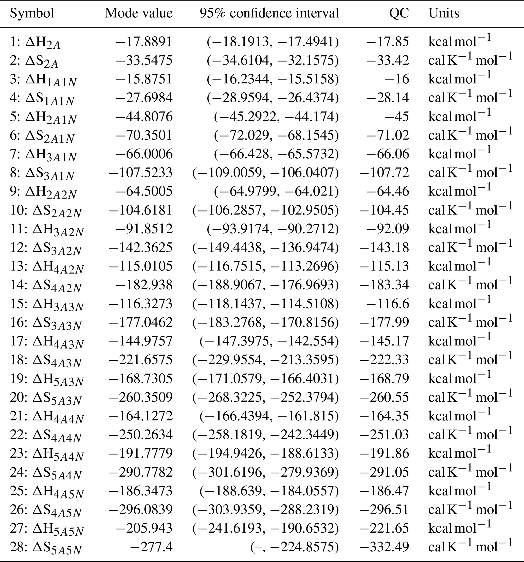

Figure D6One-dimensional marginal distributions (for parameter indexes ranging from 1 to 28) of the base 10 logarithm of the evaporation rates (units given in s−1) at temperature 278 K obtained from a posterior distribution of thermodynamic parameters (cluster formation enthalpies and entropies) determined from steady-state cluster concentration measured at temperatures 278 and 292 K. Red lines denote the baseline values from Olenius et al. (2013b) used to generate the synthetic data. The notation xAyN corresponds to a cluster with x sulfuric acid and y ammonia molecules.
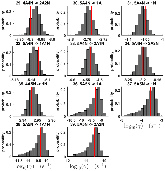
Figure D7One-dimensional marginal distributions (for parameter indexes ranging from 29 to 39) of the base 10 logarithm of the evaporation rates (units given in s−1) at temperature 278 K obtained from a posterior distribution of thermodynamic parameters (cluster formation enthalpies and entropies) determined from steady-state cluster concentration measured at temperatures 278 and 292 K. Red lines denote the baseline values from Olenius et al. (2013b) used to generate the synthetic data. The notation xAyN corresponds to a cluster with x sulfuric acid and y ammonia molecules.
Table D2Evaporation rates at temperature 278 K (units given in s−1) computed from a posterior distribution of the thermodynamic parameters (cluster formation enthalpies and entropies) which had previously been determined from the steady-state concentration measurements at temperatures 278 and 292 K. Here, the mode of distribution (in bold) is given together with the range of possible values in the parentheses. The last column presents the quantum-chemistry-based evaporation rates used for creating the synthetic data (borrowed from Olenius et al., 2013b). The notation xAyN corresponds to a cluster with x sulfuric acid and y ammonia molecules.

The code is available via the following Zenodo repository: https://doi.org/10.5281/zenodo.3766925 (Shcherbacheva, 2020).
AS produced the codes and conducted all the computational experiments for generation of the synthetic data and the MCMC parameter estimation, and prepared all the plots presented in the paper. TB, AS, TK, HV and HH are responsible for writing the manuscript. TO assisted with generation of the synthetic data, preformed sanity check of the results and gave valuable comments regarding the manuscript. TH and TB actively participated in development of the methodological approach. ML provided technical assistance with the mcmcstat toolbox which was used for MCMC simulations. JK assisted with the code compilation and debugging. HH assisted with interpretation of the MCMC results and proper usage of the DRAM computational method. TK and HV helped to interpret the outcomes of the study.
The authors declare that they have no conflict of interest
We thank the European Research Council project 692891-DAMOCLES, Academy of Finland (project no. 307331) and University of Helsinki: Faculty of Science ATMATH project for funding, Helsinki University Library for covering the open access fees and the CSC-IT Centre for Science in Espoo, Finland, for computational resources. We also thank Olli Pakarinen (Institute for Atmospheric and Earth System Research, University of Helsinki, Helsinki, Finland) for advice in plotting the synthetic data used in the present study.
This research has been supported by the European Research Council project 692891-DAMOCLES, the Academy of Finland (grant no. 307331) and University of Helsinki: Faculty of Science ATMATH project.
Open-access funding was provided by Helsinki University Library.
This paper was edited by Fangqun Yu and reviewed by two anonymous referees.
Almeida, J., Schobesberger, S., Kürten, A., Ortega, I. K., Kupiainen-Määttä, O., Praplan, A. P., Adamov, A., Amorim, A., Bianchi, F., Breitenlechner, M., David, A., Dommen, J., Donahue, N. M., Downard, A., Dunne, E., Duplissy, J., Ehrhart, S., Flagan, R. C., Franchin, A., Guida, R., Hakala, J., Hansel, A., Heinritzi, M., Henschel, H., Jokinen, T., Junninen, H., Kajos, M., Kangasluoma, J., Keskinen, H., Kupc, A., Kurtén, T., Kvashin, A. N., Laaksonen, A., Lehtipalo, K., Leiminger, M., Leppä, J., Loukonen, V., Makhmutov, V., Mathot, S., McGrath, M. J., Nieminen, T., Olenius, T., Onnela, A., Petäjä, T., Riccobono, F., Riipinen, I., Rissanen, M., Rondo, L., Ruuskanen, T., Santos, F. D., Sarnela, N., Schallhart, S., Schnitzhofer, R., Seinfeld, J. H., Simon, M., Sipilä, M., Stozhkov, Y., Stratmann, F., Tomé, A., Tröstl, J., Tsagkogeorgas, G., Vaattovaara, P., Viisanen, Y., Virtanen, A., Vrtala, A., Wagner, P. E., Weingartner, E., Wex, H., Williamson, C., Wimmer, D., Ye, P., Yli-Juuti, T., Carslaw, K. S., Kulmala, M., Curtius, J., Baltensperger, U., Worsnop, D. R., Vehkamäki, H., and Kirkby, J.: Molecular understanding of sulphuric acid-amine particle nucleation in the atmosphere, Nature, 502, 359–363, https://doi.org/10.1038/nature12663, 2013. a, b, c, d
Ball, J. M., Carr, J., and Penrose, O.: The Becker-Doring cluster equations: basic properties and asymptotic behaviour of solutions, Commun. Math. Phys., 104, 657–692, https://doi.org/10.1007/BF01211070, 1986. a
Besel, V., Kubecka, J., Kurten, T., and Vehkamäki, H.: Impact of Quantum Chemistry Parameter Choices and Cluster Distribution Model Settings on Modeled Atmospheric Particle Formation Rates, J. Phys. Chem. A, 124, 5931–5943, 2020. a, b
Bianchi, F., Tröstl, J., Junninen, H., Frege, C., Henne, S., Hoyle, C. R., Molteni, U., Herrmann, E., Adamov, A., Bukowiecki, N., Chen, X., Duplissy, J., Gysel, M., Hutterli, M., Kangasluoma, J., Kontkanen, J., Kürten, A., Manninen, H. E., Münch, S., Peräkylä, O., Petäjä, T., Rondo, L., Williamson, C., Weingartner, E., Curtius, J., Worsnop, D. R., Kulmala, M., Dommen, J., and Baltensperger, U.: New particle formation in the free troposphere: A question of chemistry and timing, Science, 352, 1109–1112, https://doi.org/10.1126/science.aad5456, 2016. a
Braak, C. J. F. T.: A Markov Chain Monte Carlo version of the genetic algorithm Differential Evolution: easy Bayesian computing for real parameter spaces, Statistics and Computing, 16, 239–249, https://doi.org/10.1007/s11222-006-8769-1, 2006. a
Brown, P. N., Byrne, G. D., and Hindmarsh, A. C.: VODE: A Variable-Coefficient ODE Solver, SIAM J. Sci. Stat. Comp., 10, 1038–1051, 1989. a
Ehn, M., Thornton, J. A., Kleist, E., Sipilä, M., Junninen, H., Pullinen, I., Springer, M., Rubach, F., Tillmann, R., Lee, B., Lopez-Hilfiker, F., Andres, S., Acir, I.-H., Rissanen, M., Jokinen, T., Schobesberger, S., Kangasluoma, J., Kontkanen, J., Nieminen, T., Kurtén, T., Nielsen, L. B., Jørgensen, S., Kjaergaard, H. G., Canagaratna, M., Maso, M. D., Berndt, T., Petäjä, T., Wahner, A., Kerminen, V.-M., Kulmala, M., Worsnop, D. R., Wildt, J., and Mentel, T. F.: A large source of low-volatility secondary organic aerosol, Nature, 506, 476–479, https://doi.org/10.1038/nature13032, 2014. a
Eisele, F. L. and Hanson, D. R.: First Measurement of Prenucleation Molecular Clusters, J. Phys. Chem. A, 104, 830–836, https://doi.org/10.1021/jp9930651, 2000. a
Elm, J. and Kristensen, K.: Basis set convergence of the binding energies of strongly hydrogen-bonded atmospheric clusters, Phys. Chem. Chem. Phys., 19, 1122–1133, 2017. a, b, c
Elm, J., Bilde, M., and Mikkelsen, K. V.: Assessment of binding energies of atmospherically relevant clusters, Phys. Chem. Chem. Phys., 15, 16442–16445, 2013. a, b
Gelman, A., Carlin, J. B., Stern, H. S., and Rubin, D. B.: Bayesian Data Analysis, 2nd edn., Chapman and Hall/CRC, 293–311, 2004. a
Haario, H., Saksman, E., and Tamminen, J.: Adaptive proposal distribution for random walk Metropolis algorithm, Computation. Stat., 14, 375–395, https://doi.org/10.1007/s001800050022, 1999. a
Haario, H., Saksman, E., and Tamminen, J.: An adaptive Metropolis algorithm, Bernoulli, 7, 223–242, available at: https://projecteuclid.org:443/euclid.bj/1080222083 (last access: 9 December 2020), 2001. a, b, c, d, e
Haario, H., Laine, M., Mira, A., and Saksman, E.: DRAM: Efficient adaptive MCMC, Stat. Comput., 16, 339–354, https://doi.org/10.1007/s11222-006-9438-0, 2006. a, b, c, d, e
Halonen, R., Zapadinsky, E., Kurtén, T., Vehkamäki, H., and Reischl, B.: Rate enhancement in collisions of sulfuric acid molecules due to long-range intermolecular forces, Atmos. Chem. Phys., 19, 13355–13366, https://doi.org/10.5194/acp-19-13355-2019, 2019 a
Hingant, E. and Yvinec, R.: Deterministic and Stochastic Becker-Döring Equations: Past and Recent Mathematical Developments, in: Stochastic Processes, Multiscale Modeling, and Numerical Methods for Computational Cellular Biology Springer International Publishing, 175–204, 2017. a
Hyttinen, N., Otkjær, R. V., Iyer, S., Kjaergaard, H. G., Rissanen, M. P., Wennberg, P. O., and Kurtén, T.: Computational Comparison of Different Reagent Ions in the Chemical Ionization of Oxidized Multifunctional Compounds, J. Phys. Chem. A, 122, 269–279, https://doi.org/10.1021/acs.jpca.7b10015, 2018. a
Junninen, H., Ehn, M., Petäjä, T., Luosujärvi, L., Kotiaho, T., Kostiainen, R., Rohner, U., Gonin, M., Fuhrer, K., Kulmala, M., and Worsnop, D. R.: A high-resolution mass spectrometer to measure atmospheric ion composition, Atmos. Meas. Tech., 3, 1039–1053, https://doi.org/10.5194/amt-3-1039-2010, 2010. a
Kirkby, J., Curtius, J., Almeida, J., Dunne, E., Duplissy, J., Ehrhart, S., Franchin, A., Gagné, S., Ickes, L., Kürten, A., Kupc, A., Metzger, A., Riccobono, F., Rondo, L., Schobesberger, S., Tsagkogeorgas, G., Wimmer, D., Amorim, A., Bianchi, F., Breitenlechner, M., David, A., Dommen, J., Downard, A., Ehn, M., Flagan, R. C., Haider, S., Hansel, A., Hauser, D., Jud, W., Junninen, H., Kreissl, F., Kvashin, A., Laaksonen, A., Lehtipalo, K., Lima, J., Lovejoy, E. R., Makhmutov, V., Mathot, S., Mikkilä, J., Minginette, P., Mogo, S., Nieminen, T., Onnela, A., Pereira, P., Petäjä, T., Schnitzhofer, R., Seinfeld, J. H., Sipilä, M., Stozhkov, Y., Stratmann, F., Tomé, A., Vanhanen, J., Viisanen, Y., Vrtala, A., Wagner, P. E., Walther, H., Weingartner, E., Wex, H., Winkler, P. M., Carslaw, K. S., Worsnop, D. R., Baltensperger, U., and Kulmala, M.: Role of sulphuric acid, ammonia and galactic cosmic rays in atmospheric aerosol nucleation, Nature, 476, 429, https://doi.org/10.1038/nature10343, 2011. a, b, c
Kupiainen-Määttä, O.: A Monte Carlo approach for determining cluster evaporation rates from concentration measurements, Atmos. Chem. Phys., 16, 14585–14598, https://doi.org/10.5194/acp-16-14585-2016, 2016. a, b, c, d, e, f
Kupiainen-Määttä, O., Olenius, T., Kurtén, T., and Vehkamäki, H.: CIMS Sulfuric Acid Detection Efficiency Enhanced by Amines Due to Higher Dipole Moments: A Computational Study, J. Phys. Chem. A, 117, 14109–14119, https://doi.org/10.1021/jp4049764, 2013. a
Kürten, A.: New particle formation from sulfuric acid and ammonia: nucleation and growth model based on thermodynamics derived from CLOUD measurements for a wide range of conditions, Atmos. Chem. Phys., 19, 5033–5050, https://doi.org/10.5194/acp-19-5033-2019, 2019. a, b, c, d, e
Kürten, A., Münch, S., Rondo, L., Bianchi, F., Duplissy, J., Jokinen, T., Junninen, H., Sarnela, N., Schobesberger, S., Simon, M., Sipilä, M., Almeida, J., Amorim, A., Dommen, J., Donahue, N. M., Dunne, E. M., Flagan, R. C., Franchin, A., Kirkby, J., Kupc, A., Makhmutov, V., Petäjä, T., Praplan, A. P., Riccobono, F., Steiner, G., Tomé, A., Tsagkogeorgas, G., Wagner, P. E., Wimmer, D., Baltensperger, U., Kulmala, M., Worsnop, D. R., and Curtius, J.: Thermodynamics of the formation of sulfuric acid dimers in the binary (H2SO4−H2O) and ternary () system, Atmos. Chem. Phys., 15, 10701–10721, https://doi.org/10.5194/acp-15-10701-2015, 2015. a, b, c, d
Kurtén, T., Torpo, L., Ding, C.-G., Vehkamäki, H., Sundberg, M. R., Laasonen, K., and Kulmala, M.: A density functional study on water-sulfuric acid-ammonia clusters and implications for atmospheric cluster formation, J. Geophys. Res., 112, D04210, https://doi.org/10.1029/2006jd007391, 2007. a
Lee, S.-H., Reeves, J. M., Wilson, J. C., Hunton, D. E., Viggiano, A. A., Miller, T. M., Ballenthin, J. O., and Lait, L. R.: Particle Formation by Ion Nucleation in the Upper Troposphere and Lower Stratosphere, Science, 301, 1886–1889, https://doi.org/10.1126/science.1087236, 2003. a
Matsugi, A.: Collision Frequency for Energy Transfer in Unimolecular Reactions, J. Phys. Chem. A, 122, 1972–1985, https://doi.org/10.1021/acs.jpca.8b00444, 2018. a
McGrath, M. J., Olenius, T., Ortega, I. K., Loukonen, V., Paasonen, P., Kurtén, T., Kulmala, M., and Vehkamäki, H.: Atmospheric Cluster Dynamics Code: a flexible method for solution of the birth-death equations, Atmos. Chem. Phys., 12, 2345–2355, https://doi.org/10.5194/acp-12-2345-2012, 2012. a, b
Metropolis, N., Rosenbluth, A. W., Rosenbluth, M. N., Teller, A. H., and Teller, E.: Equation of State Calculations by Fast Computing Machines, J. Chem. Phys., 21, 1087–1092, https://doi.org/10.1063/1.1699114, 1953. a
Mira, A.: On Metropolis-Hastings algorithms with delayed rejection, Metron – International Journal of Statistics, 0, 231–241, available at: https://ideas.repec.org/a/mtn/ancoec/2001316.html (last access: 9 December 2020), 2001. a, b
Nadykto, A. B., Herb, J., Yu, F., and Xu, Y.: Enhancement in the production of nucleating clusters due to dimethylamine and large uncertainties in the thermochemistry of amine-enhanced nucleation, Chem. Phys. Lett., 609, 42–49, https://doi.org/10.1016/j.cplett.2014.03.036, 2014. a
Olenius, T., Kupiainen-Määttä, O., Ortega, I. K., Kurtén, T., and Vehkamäki, H.: Free energy barrier in the growth of sulfuric acid-ammonia and sulfuric acid-dimethylamine clusters, J. Chem. Phys., 139, 084312, https://doi.org/10.1063/1.4819024, 2013a. a, b
Olenius, T., Schobesberger, S., Kupiainen-Määttä, O., Franchin, A., Junninen, H., Ortega, I. K., Kurtén, T., Loukonen, V., Worsnop, D. R., Kulmala, M., and Vehkamäki, H.: Comparing simulated and experimental molecular cluster distributions, Faraday Discuss., 165, 75–89, https://doi.org/10.1039/C3FD00031A, 2013b. a, b, c, d, e, f, g, h, i, j, k, l, m, n, o, p, q, r, s, t, u, v, w, x, y, z, aa, ab, ac, ad, ae, af, ag, ah
Ortega, I. K., Kupiainen, O., Kurtén, T., Olenius, T., Wilkman, O., McGrath, M. J., Loukonen, V., and Vehkamäki, H.: From quantum chemical formation free energies to evaporation rates, Atmos. Chem. Phys., 12, 225–235, https://doi.org/10.5194/acp-12-225-2012, 2012. a, b
Schobesberger, S., Franchin, A., Bianchi, F., Rondo, L., Duplissy, J., Kürten, A., Ortega, I. K., Metzger, A., Schnitzhofer, R., Almeida, J., Amorim, A., Dommen, J., Dunne, E. M., Ehn, M., Gagné, S., Ickes, L., Junninen, H., Hansel, A., Kerminen, V.-M., Kirkby, J., Kupc, A., Laaksonen, A., Lehtipalo, K., Mathot, S., Onnela, A., Petäjä, T., Riccobono, F., Santos, F. D., Sipilä, M., Tomé, A., Tsagkogeorgas, G., Viisanen, Y., Wagner, P. E., Wimmer, D., Curtius, J., Donahue, N. M., Baltensperger, U., Kulmala, M., and Worsnop, D. R.: On the composition of ammonia–sulfuric-acid ion clusters during aerosol particle formation, Atmos. Chem. Phys., 15, 55–78, https://doi.org/10.5194/acp-15-55-2015, 2015. a
Shcherbacheva, A.: AnnaShcher/Shcherbacheva_ACDP: Release 1, Version v1.0, Zenodo, https://doi.org/10.5281/zenodo.3766925, 2020. a
Vahteristo, K., Laari, A., Haario, H., and Solonen, A.: Estimation of kinetic parameters in neopentyl glycol esterification with propionic acid, Chem. Eng. Sci., 63, 587–598, https://doi.org/10.1016/j.ces.2007.09.023, 2008. a
Yan, C., Dada, L., Rose, C., Jokinen, T., Nie, W., Schobesberger, S., Junninen, H., Lehtipalo, K., Sarnela, N., Makkonen, U., Garmash, O., Wang, Y., Zha, Q., Paasonen, P., Bianchi, F., Sipilä, M., Ehn, M., Petäjä, T., Kerminen, V.-M., Worsnop, D. R., and Kulmala, M.: The role of H2SO4−NH3 anion clusters in ion-induced aerosol nucleation mechanisms in the boreal forest, Atmos. Chem. Phys., 18, 13231–13243, https://doi.org/10.5194/acp-18-13231-2018, 2018. a
Yang, H., Goudeli, E., and Hogan, C. J. J.: Condensation and dissociation rates for gas phase metal clusters from molecular dynamics trajectory calculations, J. Chem. Phys., 148, 164304, https://doi.org/10.1063/1.5026689, 2018. a
Yu, F. and Turco, R.: Ultrafine aerosol formation via ion-mediated nucleation, Geophys. Res. Lett., 27, 883–886, https://doi.org/10.1029/1999GL011151, 2000. a
Yu, F., Nadykto, A. B., Herb, J., Luo, G., Nazarenko, K. M., and Uvarova, L. A.: ternary ion-mediated nucleation (TIMN): kinetic-based model and comparison with CLOUD measurements, Atmos. Chem. Phys., 18, 17451–17474, https://doi.org/10.5194/acp-18-17451-2018, 2018. a, b
Zhao, J., Eisele, F. L., Titcombe, M., Kuang, C., and McMurry, P. H.: Chemical ionization mass spectrometric measurements of atmospheric neutral clusters using the cluster-CIMS, J. Geophys. Res., 115, D08205, https://doi.org/10.1029/2009jd012606, 2010. a
Here, stationary means that the probability of transitioning from the current state at position j to the new state at position j+1 is independent of j.
- Abstract
- Introduction
- Simulation methods
- Results and discussion
- Conclusions
- Appendix A: Mathematical overview
- Appendix B: Estimation of the evaporation rates from steady-state data
- Appendix C: Estimation of the evaporation rates from time-dependent data
- Appendix D: Estimation of the cluster formation enthalpies and entropies from steady-state concentration measurements
- Code availability
- Author contributions
- Competing interests
- Acknowledgements
- Financial support
- Review statement
- References