Ship-based measurements of ice nuclei concentrations over the Arctic, Atlantic, Pacific and Southern oceans

Ambient concentrations of ice-forming particles measured during ship expeditions are collected and summarised with the aim of determining the spatial distribution and variability in ice nuclei in oceanic regions. The presented data from literature and previously unpublished data from over 23 months of ship-based measurements stretch from the Arctic to the Southern Ocean and include a circumnavigation of Antarctica. In comparison to continental observations, ship-based measurements of ambient ice nuclei show 1 to 2 orders of magnitude lower mean concentrations. To quantify the geographical variability in oceanic areas, the concentration range of potential ice nuclei in different climate zones is analysed by meridionally dividing the expedition tracks into tropical, temperate and polar climate zones. We find that concentrations of ice nuclei in these meridional zones follow temperature spectra with similar slopes but vary in absolute concentration. Typically, the frequency with which specific concentrations of ice nuclei are observed at a certain temperature follows a log-normal distribution. A consequence of the log-normal distribution is that the mean concentration is higher than the most frequently measured concentration. Finally, the potential contribution of ship exhaust to the measured ice nuclei concentration on board research vessels is analysed as function of temperature. We find a sharp onset of the influence at approximately −36 ^∘C but none at warmer temperatures that could bias ship-based measurements.

1 Introduction

A small fraction of atmospheric aerosol particles possesses properties that induce the nucleation of ice. Herein the term ice nuclei (IN) is used to describe these particles, without specificity about their nature, equivalent to the proposed term ice nucleating particles (Vali et al., 2015). The concentration of IN active at a certain temperature affects the extent of ice crystal formation in clouds. Thereby, IN have an effect on precipitation formation, cloud optical properties and cloud persistence (e.g. DeMott et al., 2010). Stratiform clouds are more affected by the IN concentration than convective clouds because of differences in cloud water content and dynamics (Zeng et al., 2009). Since the ratio between stratiform and convective cloud amount changes meridionally, with more stratiform clouds towards higher latitudes, the effect of IN concentration on cloud properties increases from the tropical to polar regions (Zeng et al., 2009). The most important ice nucleation mechanism for mixed-phase clouds is immersion freezing. The temperature range of immersion freezing, in which IN are first immersed in supercooled droplets before triggering ice formation, is limited at the lower end by the onset temperature of homogeneous ice nucleation (−38 ^∘C), below which droplets freeze without the necessity for catalysing IN. At the high end, exceptionally efficient, biological IN are known to nucleate ice at temperatures as high as −1.3 ^∘C (Schnell and Vali, 1972), whereas, for example, submicron desert dust IN typically show high activity only below −25 ^∘C (Boose et al., 2016). After the onset of immersion freezing, the glaciation of mixed-phase clouds can be enhanced by secondary ice formation, a cascade process in which supercooled droplets freeze and shatter on contact with ice crystals (Mason and Maybank, 1960) or by ejection of ice splinters during the formation of rime on graupel (Hallett and Mossop, 1974).

To describe the atmospheric IN population comprehensively, IN concentrations in the entire temperature range of immersion freezing (0 to −38 ^∘C), their temporal fluctuation and geographical variation should be considered. The first summary and parameterisation of the change in IN concentration as a function of temperature was given by Fletcher (1962), based on a collection of ambient measurements available at the time. Even before Fletcher’s parameterisation, efforts had been made to quantify the concentration of atmospheric IN dependent upon air mass origin and weather conditions. For example, Findeisen and Schulz (1944) determined an IN temperature spectrum for central Europe on the basis of 8 years of aircraft and ground-based observations. The spatially most comprehensive measurements so far have been achieved by coordinated, ground-based measurements (e.g. Bigg and Stevenson, 1970), aircraft campaigns (e.g. DeMott et al., 2010) and ship-based observations in the Southern Ocean between Australia and Antarctica (Bigg, 1973). As 71 % of the Earth's surface is covered by oceans, ship-based observations offer an effective way of covering large areas. The Bigg (1973) data set, averaging 3 years of observations (shown in Fig. 1), has been used as a reference with which modelled IN concentrations have been validated (e.g. Vergara-Temprado et al., 2017).

We present a summary of ship-based measurements from the literature and extend this data set with unpublished data dating back as far as 1996 and measurements from several recent ship expeditions. A summary of expedition objectives can be found in Appendix A. The recent data sets were obtained during expeditions in the Arctic (Polarstern – PS 106), the Southern Ocean (Antarctic Circumnavigation Expedition – ACE) and during Atlantic transects (ACE; PS 95 and PS 79). Previously unpublished −15 ^∘C data include observations from the Pacific Ocean (SHIpborne Pole to Pole Observations – SHIPPO; U.S. Department of Energy's Atmospheric Radiation Measurement (ARM) Cloud Aerosol Precipitation Experiment – ACAPEX), Southern Ocean (TAN1502) and central Arctic Ocean (Arctic Ocean Expedition – AOE-96 and AOE-2001).

2 Sampling and measurement

Ship-based measurements of IN concentration record the abundance of potential IN in the marine boundary layer, some metres above sea level. Much of the available literature data are limited to IN concentrations at −15 or −20 ^∘C because of instrumental limitations and a focus on the influence of IN abundance on precipitation formation. During recent expeditions, emphasis was put on collecting data covering a broad temperature range (0 to −38 ^∘C) because of a shift in focus to the cloud radiative effect and the realisation that even low IN concentrations can have a large effect by triggering secondary ice formation (e.g. Sullivan et al., 2018). Additional to the importance for cloud microphysics, observations over a broader temperature range allow the construction of IN temperature spectra, providing information on the abundance of potential IN sources from their slope (e.g. Welti et al., 2018).

Two measurement techniques were used for the recent ship-based measurements. First, continuous flow diffusion chambers (CFDCs), e.g., the Colorado State University (CSU) CFDC measuring during the Clouds, Aerosols, Precipitation Radiation and atmospherIc Composition Over the southeRN ocean campaign (CAPRICORN; McCluskey et al., 2018a), or SPectrometer for Ice Nuclei (SPIN; Droplet Measurement Technologies) measuring during the PS 95 and PS 106 cruises. CFDCs cover the low temperature range from approximately −38 to −24 ^∘C. Second, drop freezing techniques, using aerosol collected on filters during expeditions for off-line determination of the IN concentration. Drop freezing techniques typically cover the temperature range from −26 to 0 ^∘C.

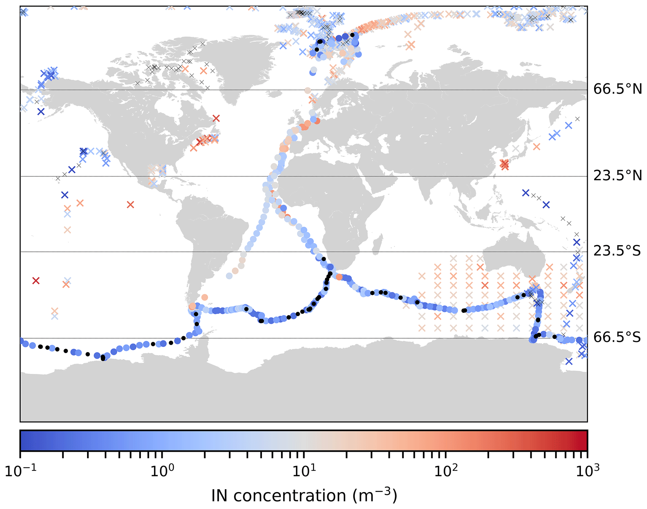
Figure 1 World map showing the locations where IN concentration data at −15 ^∘C are available from ship-based measurements. Literature data from Bigg (1973), Schnell (1977), Borys (1983), Rosinski et al. (1986), Rosinski et al. (1988, 1995), DeMott et al. (2016), McCluskey et al. (2018a), Si et al. (2018), Irish et al. (2019), Creamean et al. (2019) and unpublished data from AOE, TAN1502, ACAPEX and SHIPPO are marked as crosses. Data from ACE, PS 79, PS 95 and PS 106 are marked as circles. The symbols are colour coded according to the colour bar below the map, indicating the measured IN concentrations. Locations where the observed IN concentration was below the detection limit (< sample volume⁻¹; see Table A1) are marked in black. Climate zones are divided by horizontal lines; their fraction of the Earth's surface area can be found in Table B1.

For the new data sets in the Arctic, Atlantic and Southern Ocean (marked as circles in Fig. 1), sampling was conducted on board the research vessels (RVs) Polarstern (expeditions indicated with PS) and Academik Tryoshnikov (during the ACE campaign). For a description of the ACE and PS 106 (Physical Feedbacks of Arctic Boundary Layer, Sea Ice, Cloud and Aerosol – PASCAL) expeditions, we refer to Appendix A and references therein. On board both vessels we used the upper deck (monkey bridge), about 30 m above the ocean surface, to install the sampling devices. SPIN sampled from within a container through a whole air inlet system with subsequent drying of the aerosol. The SPIN measurement strategy was to sample 30 min intervals at a constant temperature (selected between −38 and −24 ^∘C) and constant relative humidity (85 %, 95 % or 103 % with respect to water). Each sampling condition was repeated three times within 24 h. This allowed measurements of IN concentrations at different temperatures and relative humidity with a high spatial coverage. Measurements above water saturation, representing the immersion freezing mode, are reported here. Filter samples were collected during 8 h intervals using a low volume aerosol sampler (DPA14; Digitel) with a PM₁₀ inlet during ACE and PS 106. During PS 79 and PS 95, 24 h filter samples were collected using a high volume aerosol sampler (DHA-80; Digitel) with a PM₁ inlet. The latter used 150 mm quartz fibre filters, from which 103 subsamples were extracted. IN concentration was examined in a drop freezing array setup, similar to the technique used by Conen et al. (2012) and previously described in Welti et al. (2018). With the low volume sampler, 8 h samples were collected on 47 mm diameter Nuclepore polycarbonate membranes (Whatman) with a pore size of 0.2 µm. Field blanks, which had undergone the same handling except for aerosol collection, were collected regularly to determine the filter background. Filters were stored in a −20 ^∘C cold room on board and kept cool during transport to TROPOS (the Leibniz Institute for Tropospheric Research) before storage at −20 ^∘C until analysis. To determine IN concentrations, membrane filters are immersed in 10 mL of ultra pure water to extract collected particles, and a total of 96 aliquots (each 50 µL) of the sample solution were subsequently examined in a drop freezing assay. IN concentrations are estimated from the number of frozen aliquots at a specific temperature according to Vali (1971). Data at −15 ^∘C from AOE, TAN1502, ACAPEX and SHIPPO were also obtained from filter samples. TAN1502, ACAPEX and SHIPPO filters were analysed using the CSU Ice Spectrometer (IS; Hill et al., 2016). Collection (open-faced, 0.2 µm pore filters) and processing protocols for the IS are as described in McCluskey et al. (2018a, b). During these expeditions, IN concentrations were measured over a broader temperature range, and results will be reported elsewhere. A discussion of the membrane filter technique used to determine IN concentrations during AOE can be found in Bigg (1990). Table A1 provides an overview of the location, on-board equipment, sampling time intervals and sampled air volume during expeditions from which data are included. An analysis showing that contamination from the ship's exhaust had no influence on ship-based IN concentration measurements during PS 106 and ACE is presented in Sect. 6 and Appendix C.

3 Worldwide coverage of maritime observations

Figure 1 summarises all available data at −15 ± 1 ^∘C from the literature and recent expeditions. This temperature is chosen to include observations from the literature (e.g. Bigg, 1973; Schnell, 1977; Borys, 1983; Rosinski et al., 1986, 1988, 1995) for some of which only −15 ^∘C data are available. Literature data cover the Southern Ocean, the North Atlantic off the coast of Nova Scotia, the Greenland Sea, the Pacific Ocean, the Gulf of Mexico and the East China Sea. Note that although the spatial coverage of the literature data is broad, the number of data points reported is low and often only average values were given. Recent expeditions added data from the Atlantic, Pacific, Southern and Arctic oceans. As yet unexplored regions, in terms of ship-based measurements of IN concentration, remain, e.g. the Indian Ocean, the Southeast Pacific or the Mediterranean Sea.

4 Geographic variability

Regional variations of IN concentrations on the continents coincide with strong local sources (e.g. Isono et al., 1959; DeMott et al., 2003) or IN-generating events (e.g. McCluskey et al., 2014; Suski et al., 2018). In remote maritime environments, the sources of the most common IN type by concentration can be the long-range transport of mineral dust (e.g. Bigg, 1973) or the oceans themselves. Oceans have been identified as a source of IN (e.g. by Brier and Kline, 1959; Schnell and Vali, 1975; Ickes et al., 2020) able to produce IN with a broad temperature spectrum (DeMott et al., 2016). Based on numerical simulations, Burrows et al. (2013) suggested that, in remote oceanic areas, the absence of mineral dust means that maritime IN determine the impact of heterogeneous ice formation on clouds. McCluskey et al. (2019) reported that the contribution of mineral dust or maritime aerosol changes depending on season and altitude, with strong variations from day to day. During AOE-91 and AOE-96, Bigg and Leck (2001) found evidence for a microbiological, marine source of Arctic IN with a strong seasonal dependence and a correlation with the concentration of dimethyl sulfide (DMS), a metabolite in some marine algae. They observed that IN concentrations start decreasing very rapidly after mid-September to being virtually zero by late October.

Due to the different conditions (temperature and wind speed) and location (e.g. proximity to deserts) of different parts of the world's seas and oceans, meridional variations in the IN temperature spectrum (Sect. 5) could be expected. Effects of atmospheric transport and local sources include, for example, the westward transport of large amounts of dust from the Sahara desert, higher biological productivity along coasts and at higher latitudes and furious storm tracks or sea ice cover that promote or prevent wave-derived aerosol generation.

A comparison of continental and maritime IN concentrations observed at −15 ^∘C, from the surface-based measurements in the study of Bigg and Stevenson (1970) and meridional averages of ship-based data from Fig. 1, is shown in Fig. 2. The averaging zones of Fig. 2b are indicated in Fig. 1 and defined in Table B1. Concentrations over the ocean are lower than the reported average concentrations over continents, and the variation is higher. The continental data set consists of measurements taken in the same year and season with one type of sampling device and analysis method, while ship-based measurements are a compendium of data obtained with different methods over decades, which could add to the variability in the ship-based data set. In Fig. 2b, with the exception of clearly lower IN concentrations in the S polar zone, the average IN concentration further north (S temperate to N polar) shows low zonal dependence at −15 ^∘C. In accordance with this, surprisingly similar concentrations on different continents have been found in the coordinated attempt to measure IN concentrations globally (simultaneous sample collection at 44 locations; Bigg and Stevenson, 1970). However, some contemporary data (e.g. Mason et al., 2016; DeMott et al., 2017) suggest that the values from Bigg and Stevenson (1970) may underestimate the present magnitude and range typifying the boundary layer over continental North America and Europe by a factor of 3 or more, while other data, e.g. in the eastern Mediterranean region, remain consistent with the prior assessment (Gong et al., 2019).

In general, the highest concentrations of an ice active aerosol are found at its source, and concentrations decrease with increasing distance away from the source due to random dilution with IN-free air during transport (Anderson et al., 2003). An increase in dilution time can have the same effect as transport. Random dilution causes concentrations to vary, even at a fixed position relative to the source (Ott, 1990). The higher concentration and smaller variation range of continental IN concentrations could indicate proximity to the sources (minimal dilution), while the IN population on the ocean is more diffuse, suggesting extended random dilution during transport or low, fluctuating source strength.

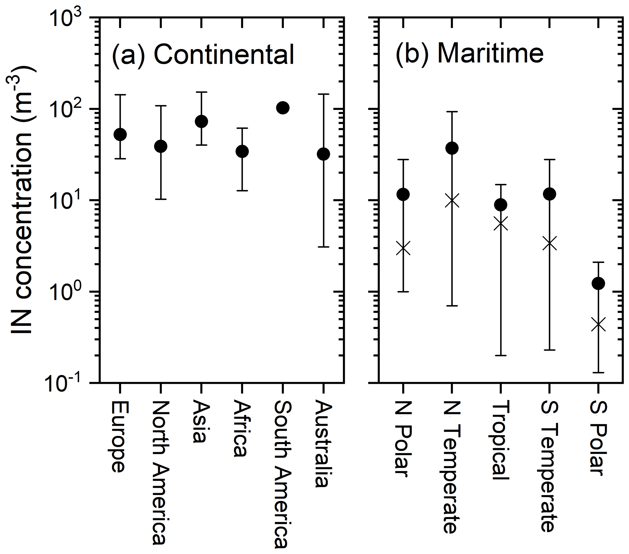
Figure 2 (a) Regionally averaged continental IN concentrations at −15 ^∘C (surface-based measurements, Bigg and Stevenson, 1970). (b) Meridionally averaged maritime IN concentrations at −15 ^∘C (shown as dots). Vertical bars indicate the concentration range where 80 % of observations lay, excluding the 10 % highest and 10 % lowest values. Most frequently measured (mode) concentrations are indicated by crosses. Continental concentrations in (a) are higher, with a lower variability than maritime IN concentrations in (b).

5 Temperature spectra

The ship-based data are used to construct zonal temperature spectra of IN concentrations and to investigate the frequency with which concentrations are measured (shown in Fig. 3). The ambient temperature spectrum at any location is a superposition of IN contributions from several sources activating at specific temperatures. As different sources can contribute IN that are active at different temperatures, a change in nearby sources and source strength can generate a change in the temperature spectrum shape (see Bigg, 1961; Welti et al., 2018 for a discussion of temperature spectrum features). In the ship-based data, examples of non-monotonic temperature spectra with step-like features were observed close to continents, e.g. elevated IN concentration at −15 ^∘C in the vicinity of harbours in Fig. 1. An increased slope at about −10 ^∘C in the meridional averaged temperature spectra is found in the tropics (measurements 350–680 km off the coast of West Africa; see Fig. 1), suggesting a local source that sometimes contributes IN that are active in this temperature range. Excluding these occasional observations of steps in the temperature spectra (occurring in ≤5 % of observations; see Fig. 3), we find a consistent exponential increase in the IN concentration with decreasing temperature, in all climate zones, and with only a small variation in slope on a log scale.

On the left column of Fig. 3, the meridional separated temperature spectra of data collected during PS 79, PS 95, PS 106 and ACE are shown. Data measured with the CSU CFDC during CAPRICORN are included in the S temperate zone. At −15 ^∘C, IN concentrations from all additional data sets (see Table A1) are also shown to compare the range in which ambient concentrations vary. The normalised frequency with which concentrations occur at each temperature in the temperature spectra is shown in the right column of Fig. 3. The symmetry of contours in Fig. 3 and the offset of mean concentrations from the centres of the ranges in Fig. 2b suggest that concentrations follow normal distributions when plotted on a log scale, indicating an underlying log-normal distribution. It has previously been noted that the frequency with which specific IN concentrations are observed follows such a distribution (described in Isaac and Douglas, 1971; Welti et al., 2018). Two consequences of the log-normal frequency distribution can be seen in Fig. 3. While the complete data set (left column of Fig. 3) shows a spread over 3 to 4 orders of magnitude, frequently measured concentrations (≥20 %) are confined to a range of less than 1 order of magnitude (reddish colours in the right column of Fig. 3). Note that at temperatures where data are sparse, high-frequency occurrence is biased towards the available data points, which may compromise its reliability. Within the range of the most frequent concentrations (yellow and reddish colours in the right column of Fig. 3) the temperature-dependent change in IN concentration, i.e. the slope of the IN concentration versus the temperature, is similar for all five meridional zones, and the absolute concentration changes by less than 2 orders of magnitude between zones. The skewed (log-normal) frequency distribution causes the mode (most frequently measured IN concentration) to be less than the arithmetic mean. Therefore, individual concentration measurements are often below the average concentrations.

The temperature above which it becomes most probable to measure no IN in a sample of approximately 10 m³ (the highest frequency on the zero line in the right column of Fig. 3) is at −14 ^∘C in the N polar, S polar and the S temperate zones. In contrast, the temperature threshold in the Tropical and N temperate climate zone is found between −10 and −9 ^∘C.

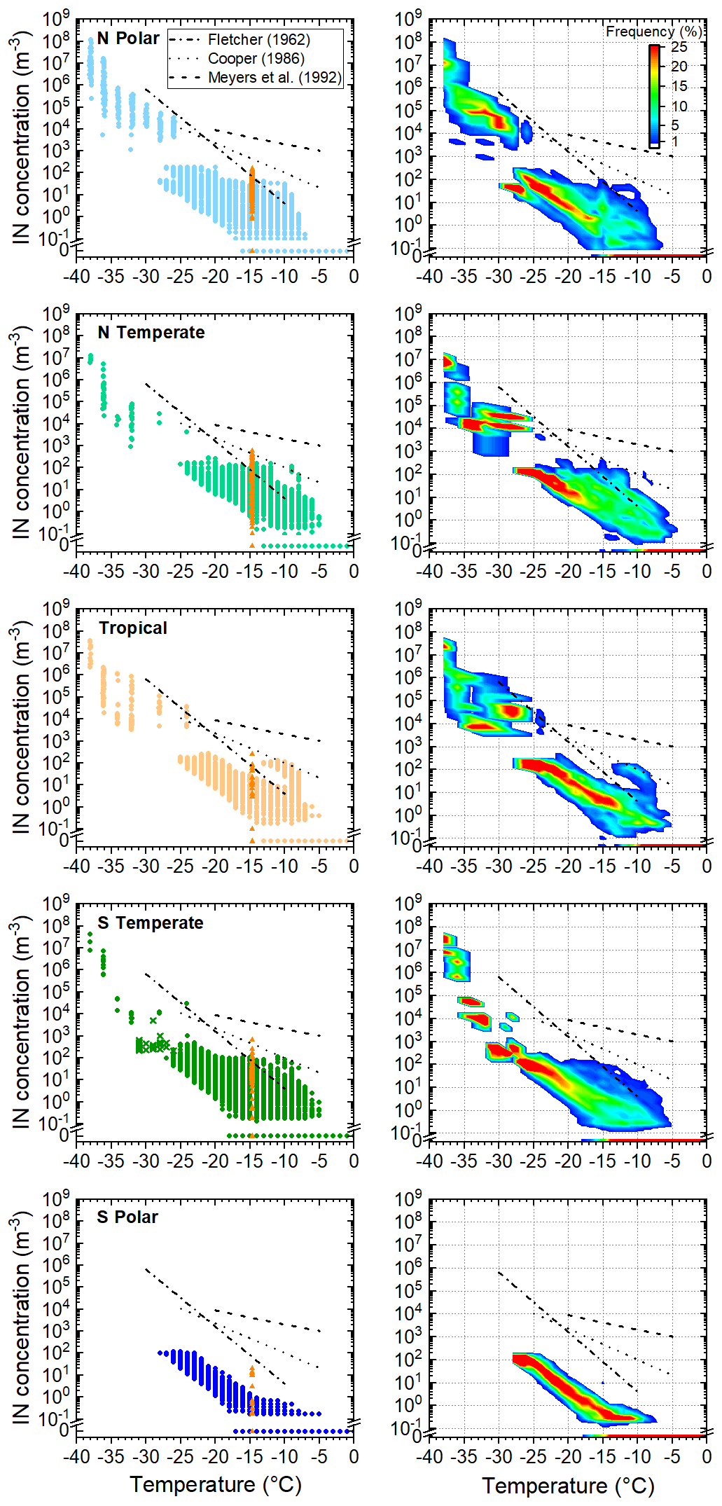
Figure 3 Top-down maritime data are stratified into N polar, N temperate, Tropical, S temperate and S polar zones (as indicated in Fig. 1). The left column shows the meridional temperature spectra of observed IN concentrations. Data from recent expeditions (ACE, PS 95 and PS 106) are shown as circles. In the S temperate zone, CSU CFDC data from CAPRICORN are shown as crosses. Literature data at −15 ^∘C (the same are shown as crosses in Fig. 1) are overlaid as orange triangles for comparison. The right column shows the frequency of occurrence of measured concentrations at each temperature (1 ^∘C temperature bins). While the total variation in IN concentration at a certain temperature is large, there is a range of approximately 1 order of magnitude containing the most frequently (≥20 %) measured concentrations (reddish colours). The frequency with which no IN are detected is shown on the zero line. Only small, meridional differences in absolute IN concentration and the slope of the temperature-dependent change can be identified. The three often used parameterisations from Fletcher (1962), Cooper (1986), Meyers et al. (1992) are given for comparison.

Figure 4 IN vs. soot concentration (10 s averages) measured during PS 106. Dashed 1:1 lines indicate equal soot and IN concentrations. The temperature at which the IN concentration was measured is indicated in the upper left corner of each sub-figure, and the Pearson correlation of the soot and IN concentration is given on top. Moderate correlation is found at −36 ^∘C.

6 Contamination from ship exhaust

To avoid contamination during ship-based measurements, the aerosol inlet and filter sampling devices are placed in front of the ship's chimney towards the bow of the ship. In situations in which the wind speed from the rear exceeds the speed of the ship, i.e. relative wind direction from the chimney towards the sampling location, high concentrations of ship exhaust aerosol particles are encountered. Moderate contamination by turbulent mixing is also observed at relative wind speed close to zero. The potential contribution of ship exhaust particles is determined by comparing IN concentration measured with SPIN to soot particle concentration measured with a single particle soot photometer (SP2; Droplet Measurement Technologies). Figure 4 shows the concentration of soot versus IN concentration, both binned to common 10 s intervals. Moderate correlation is found at −36 ^∘C, whereas soot concentration is higher than the IN concentrations at higher temperatures and lower at lower temperatures. Comparing the temperature spectra in Fig. 3, where a distinct increase in IN concentration at −36 ^∘C can be seen, confirms that ship exhaust potentially distorts the ambient temperature spectrum at and below, but not above, −36 ^∘C. Increased concentrations at −38 ^∘C could be caused by the onset of homogeneous freezing. The influence at only the lowest temperatures indicates that the effect of contamination from ship exhaust on the immersion freezing experiments with filter samples is negligible. Figure C1 in Appendix C confirms that there is no effect of sampling air coming from the direction of the chimney of the ship on filter measurements at $T\ge -\mathrm{20}$ ^∘C. It can be argued that, at temperatures above −36 ^∘C, the effect of soot (if any) could be a suppression in the activity of other particles by covering their ice active sites (Mossop and Thorndike, 1966). Note that the present analysis is valid for the RV Polarstern exhaust. Other type of fuel or ship engines might yield a different result (Thomson et al., 2018). However, Schnell (1977) also tested a possible contamination from the exhaust of the USNS Hayes by purposely exposing membrane filters to the exhaust plumes from the galley and engines and found no IN from either source active at −15 ^∘C. McCluskey et al. (2018a) also found no statistically significant difference due to varying black carbon levels from exhaust contamination at temperatures between −16 and −26 ^∘ C on board the RV Investigator during the CAPRICORN campaign.

7 Discussion

The maritime IN concentration data presented here can be used to predict the temperature spectra in a range of oceanic regions. This can help the future development of measurement techniques and sampling strategies. As an example, to avoid artefacts from the sensitivity range of measurement techniques, the sample volume and probed temperature range need to be matched. In the current data set, the narrowing of variations below −20 ^∘C in the filter measurements from the temperate climate zone (Fig. 3, right column) is an artefact caused by the upper limit of detectable concentrations and can be avoided by sampling smaller volumes and by using dilutions of filter suspensions. In general, the sample volume and sampling time over which the concentration is averaged to one data point affects the absolute value and the variability between measurements. Smaller sample volumes result in a larger scattering of the data within experimental detection limits, including measurements of practically zero alternating with high concentrations at the upper detection limit. The smaller the sample volume, the higher the limit of detection and vice versa, i.e. larger sample air volumes allow the detection of low concentrations, while smaller sample volumes are more suitable for accessing high concentrations.

To develop parameterisations, concentrations averaged to scales required for the application should be used (Gultepe et al., 2001). Grid-box scales in numerical models are much larger than the practical sampling volume of ambient measurements. As averaging any distribution of concentrations by means of probing larger air volumes or averaging collected samples over time converges to the arithmetic mean concentration, the mean IN concentration (shown in Fig. 2b for −15 ^∘C in five climatic zones and in Fig. 5a averaged over each hemisphere) is the correct input value for large-scale numerical models, even if it is not the most frequently measured (mode) concentration. This also underscores the importance of using sufficiently large data sets for parameterisation development to avoid bias.

The frequency distributions in the right column of Fig. 3 illustrate that, within the sample volumes where IN concentrations can be measured, low values are more frequent than high values. Averaging concentrations from a skewed (log-normal) frequency distribution results in mean concentrations higher than the most frequently measured concentration. Figure 5 depicts the temperature spectra of the (a) average and (b) most frequently measured IN concentrations in the Northern Hemisphere and Southern Hemisphere. The discrepancy between the averaged and most frequently measured concentrations is most pronounced for low concentrations. Within the sensitivity limits of the measurements presented here, often no IN are detected above −15 ^∘C in 10 m³ of maritime air.
Between −25 and −30 ^∘C, a jump in the Northern Hemisphere temperature spectra can be seen in Fig. 5. It could be speculated that the jump coincides with the temperature at which mineral dust particles start to exert a strong influence (e.g. Boose et al., 2016) and the N–S difference could be due to more dust-emitting land masses in the north. Another reason for the jump could be that it is an artefact from the combination of filter measurements reaching their upper detection limit, with SPIN measurements reaching their lower detection limit in this range of IN concentration. Further measurements and the development of measurement techniques that can bridge this gap are needed.

In Fig. 1 a clear change towards lower IN concentrations measured recently in the Southern Ocean and the literature values from Bigg (1973) can be seen. Bigg reported averaged concentrations measured in 5×5^∘ sectors. Noting the log-normal frequency distribution of observed IN concentrations, the offset between the average and most frequently occurring concentrations at −15 ^∘C (see Fig. 5) could be one factor that helps to explain the difference. A decline in IN abundance in the Southern Ocean over the last few decades (suggested by Bigg, 1990) could be another reason.

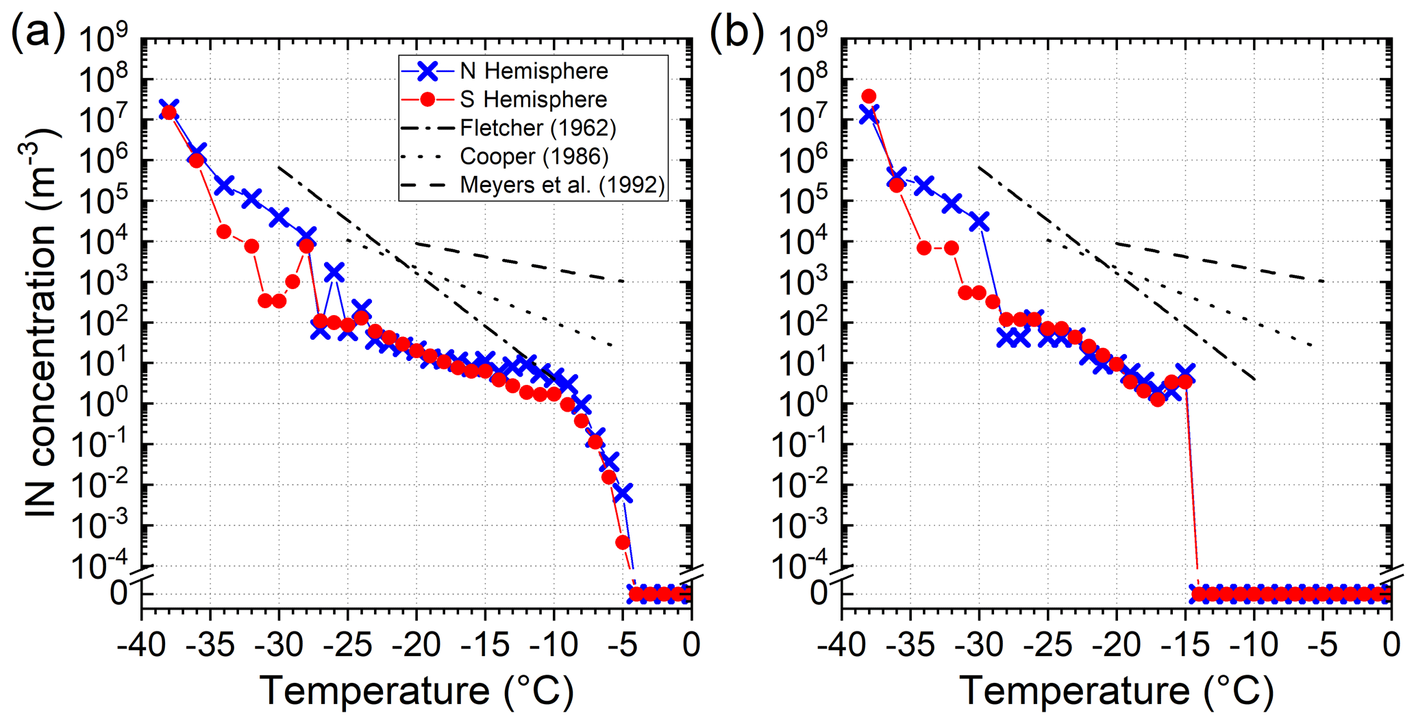
Figure 5 (a) Comparison of the average IN concentration between the Northern and Southern hemispheres' oceanic regions. (b) Comparison of the most frequently observed IN concentrations in the Northern and Southern hemispheres' oceanic regions. Parameterisations from Fletcher (1962), Cooper (1986) and Meyers et al. (1992) are given for comparison. The average IN concentrations over both hemispheres, shown in (a), can be approximated by IN (m⁻³) $=\left(T\right({}^{\circ }\mathrm{C})+a)\cdot (-b\cdot \exp (c/\left(T\right({}^{\circ }\mathrm{C})+d)\left)\right)$, with $a=\mathrm{5}{}^{\circ }\mathrm{C},b={\mathrm{10}}^{-\mathrm{5}}{\mathrm{m}}^{-\mathrm{3}}{}^{\circ }{\mathrm{C}}^{-\mathrm{1}},c=\mathrm{500}{}^{\circ }\mathrm{C},d=\mathrm{60}{}^{\circ }\mathrm{C}$, for $-\mathrm{36}{}^{\circ }\mathrm{C}<T<-\mathrm{5}{}^{\circ }\mathrm{C}$.

8 Conclusions

Ship-based observations are an efficient strategy for obtaining measurements, with a wide spatial coverage, representing IN characteristics over the (remote) maritime environment, distant from continental sources. The present study provides a summary of IN concentrations observed during ship expeditions in the last 50 years in different oceanic regions. This overview can be used to validate parameterisations of IN concentrations in numerical climate models (see data availability below) and to plan future expeditions.

In the data presented here, the lowest IN concentrations are observed in polar regions and highest in the temperate climate zones. The overall geographical variation in maritime IN concentration is surprisingly small (below 2 orders of magnitude). A zonal difference was found in the temperature above which, most frequently, no IN are detected (−9 ^∘C in N temperate and −10 ^∘C in Tropical but much colder at −14 ^∘C in S temperate, N polar and S polar climates). The largest difference between the Northern Hemisphere and Southern Hemisphere is found at temperatures below −28 ^∘C, where IN concentrations are higher in the Northern Hemisphere. This coincides with the temperature range where desert dust particles become especially active ice nuclei.

A comparison of ship-emitted soot and IN concentrations shows that contamination from ship exhaust does not bias IN concentration measurements at temperatures above −36 ^∘C.

Recent maritime ice nucleation measurements show lower IN concentrations compared to the reported mean values from the 1970s to the 1980s. Apart from the possibility of an actual decrease in the maritime IN concentration, the log-normal frequency distribution of measured IN concentrations could account for part of the difference in this direction. Individual observations of a variable following a log-normal frequency distribution are most frequently lower than the arithmetic mean. This can also be one reason for the difference between recent observations and, for example, the Fletcher (1962) parameterisation for IN concentrations which is based on older data that have been reported as mean values.

To establish an unbiased climatology of IN concentration in the maritime environment, measurements aiming to extend the spatial coverage and to capture the temporal variability in IN are needed, e.g. to capture the dependence on marine productivity, season, meteorology, special aerosol emissions and to identify IN sources. To achieve these goals, continued efforts to include ice nucleation measurements as important observations on board of scientific expeditions are needed.

Appendix A: Overview of expeditions contributing data

Table A1 gives an overview of all expeditions that contributed data sets, when and where they took place and how IN concentration was obtained. In the following, the expeditions from which IN concentration data are reported for the first time (indicated by an asterisk in Table A1) are briefly described. References to more detailed information on expeditions and expedition reports are included.

The Antarctic Circumnavigation Expedition (ACE) from November 2016 to March 2017 was the first expedition carried out by the Swiss Polar Institute. On board the Russian RV Akademik Tryoshnikov, the voyage started with the transit from Bremerhaven, Germany, to Cape Town, South Africa, from where on the Antarctic continent was circumnavigated in three legs, including leg 1 from Cape Town to Hobart, New Zealand; leg 2 Hobart to Punta Arenas, Chile; and leg 3 Punta Arenas to Cape Town. The final segment of the expedition was the return from Cape Town to Bremerhaven. ACE included atmospheric, glaciological, oceanographic, biological and biochemical observations for a better understanding of Antarctica's ecosystem and the interplay of sea and atmosphere in the Southern Ocean (Walton and Thomas, 2018; Schmale et al., 2019).

The PS 106 campaign to the Arctic (PS 106/PASCAL in the framework of AC³; Wendisch et al., 2018) on board the RV Polarstern was from 23 May to 20 July 2017. For the first leg of the campaign, Polarstern set off from Bremerhaven, Germany, towards the Arctic Sea to establish an ice camp and drift with the ice shelf north of Svalbard. During the second leg, Polarstern cruised the sea northeast of Svalbard. The expedition ended in Tromsø, Norway. Oceanographic, atmospheric and biological observations were conducted during both legs (Macke and Flores, 2018).

The PS 95 campaign on board RV Polarstern was an Atlantic transit cruise (29 October–3 December 2015) from Bremerhaven, Germany, to Cape Town, South Africa. Observations included biological oceanography, atmospheric aerosol and remote sensing (Knust and Lochte, 2016).

The PS 79 campaign (ANT-XXVIII/5) on board RV Polarstern left Punta Arenas, Chile, on 11 April 2012 to cross the Atlantic Ocean and reach Bremerhaven, Germany, on 16 May 2012. The transect was used for biological, atmospheric and marine observations and to measure sea–atmosphere fluxes (Bumke, 2012). AOE-96 was the Arctic Ocean Expedition departing from Gothenburg, Sweden, on a Swedish RV, the icebreaker Oden. The expedition lasted from July to September 1996. During the first leg, observations were taken in the Barents Sea and the pack ice of Nansen and Amundsen basins, including an ice camp. On the second leg, the expedition reached the North Pole before sailing back to Gothenburg, Sweden. Observations included chemical and physical atmospheric measurements, meteorology, biochemical measurements and seawater chemistry (Leck et al., 2001).

AOE-2001 was an interdisciplinary Arctic Ocean Expedition on the Swedish RV Oden. Departing on 29 June 2001 from Gothenburg, Sweden, the cruise reached the pack ice north of Svalbard and continued to the North Pole. A 3-week ice camp was established on the way back, and the expedition concluded on 26 August. The observational programme included marine biology, atmospheric chemistry, aerosol chemistry and physics, meteorology, oceanography and seismology (Leck et al., 2004).

TAN1502 refers to the New Zealand–Australia Antarctic Marine Ecosystems Voyage of the NIWA RV Tangaroa vessel, which occurred from 28 January to 15 March 2015, sailing from Wellington, New Zealand, to the Ross Sea and back. The main objective of this voyage was to gather baseline ecosystem information prior to the establishment of the world's largest marine protected area located in the Ross Sea region of Antarctica in 2017 that is legislated to be in place for 35 years. The voyage included underway oceanographic and atmospheric observations.

ACAPEX was the U.S. Department of Energy's Atmospheric Radiation Measurement (ARM) Cloud Aerosol Precipitation Experiment. Samples were collected on the NOAA RV Ronald H. Brown, from 14 January to 10 March 2015, while sailing between Honolulu, Hawaii, and San Francisco, California (DeMott and Hill, 2016).

The SHIpborne Pole to Pole Observations (SHIPPO) included two campaigns, SHIPPO-2012 and SHIPPO-2014, both of which occurred on the Korean Polar Research Institute's Araon vessel. SHIPPO-2012 was conducted in July 2012, sailing from Incheon, South Korea, to Nome, Alaska, USA (DeMott et al., 2016, see the Supplement for data). SHIPPO-2014 sailed from Incheon, South Korea, to Christchurch, New Zealand.

Table A1 List of ship expeditions during which IN concentrations were measured. References indicate publications that reported IN concentrations. Note: ¹ Schnell (1977); ² Schacher (1976); ³ Bigg (1973); ⁴ Borys (1983); ⁵ Rosinski et al. (1986); ⁶ Rosinski et al. (1988); ⁷ Rosinski et al. (1995); ⁸ Bigg (1996); ⁹ Bigg and Leck (2001); ¹⁰ McCluskey et al. (2018a); ¹¹ Si et al. (2018); ¹² Irish et al. (2019); ¹³ Creamean et al. (2019); ^* New IN data set.

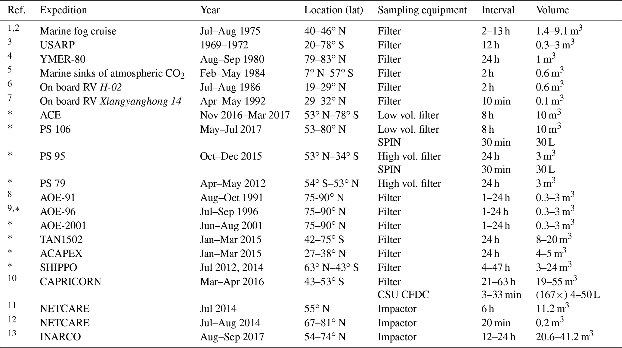
Note: RV – research vessel; USARP – United States Antarctic Research Program; YMER-80 – the Swedish Arctic Expedition 1980 on board the ice-breaker Ymer; CAPRICORN – Clouds, Aerosols, Precipitation Radiation and atmospherIc Composition Over the southeRN ocean; NETCARE – Network on Aerosols and Climate; INARCO – Ice Nucleation over the ARCtic Ocean.

Appendix B: Latitudinal subdivision of ship-based observations

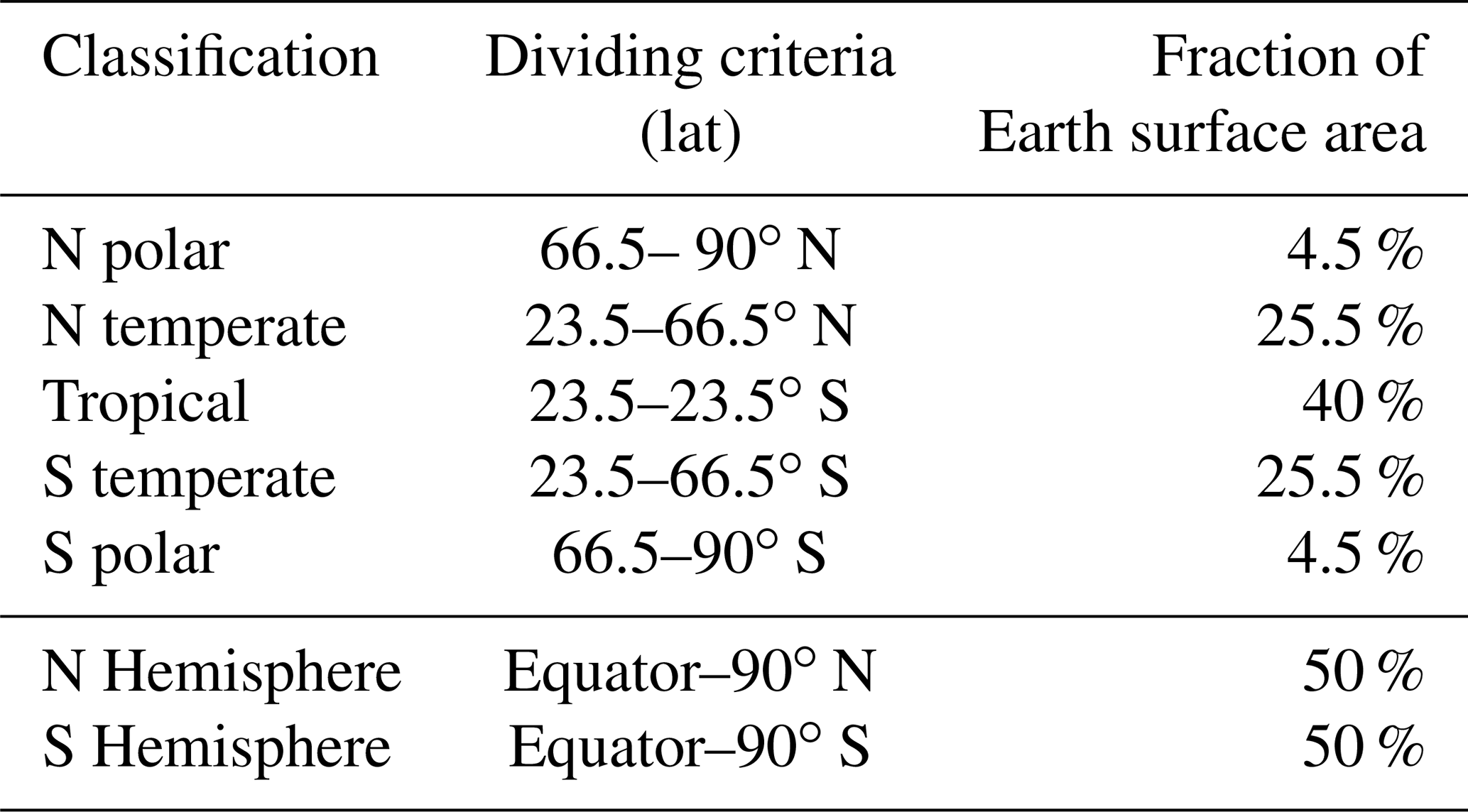
Along the cruise tracks, sample locations are subdivided into five general climate zones (Table B1) to investigate the average IN concentration at −15 ^∘C (shown in Fig. 2) and zonal temperature spectra (shown in Fig. 3). Differences between IN concentrations over the Northern Hemisphere and Southern Hemisphere in comparison to three often used parameterisations are shown in Fig. 5.

Table B1 Latitudinal subdivision of data sets.

Appendix C: Influence of ship exhaust on IN concentration at $T\ge -\mathrm{20}$ ^∘C

The sampling time in wind direction of the ship exhaust emission is compared to the concentration of IN collected on 8 h filter samples. Figure C1 shows the IN concentration in dependence on the duration of sampling from the ship exhaust at −20, −15 and −10 ^∘C. The data show no correlation, indicating that the ship's exhaust does not affect the measured IN concentration at these temperatures. This is in accordance with the data in Fig. 4, showing that ship emissions only contribute to the IN temperature spectrum at temperatures below −36 ^∘C.

Figure C1 IN concentration vs. sampling time in ship exhaust. Measured IN concentrations at −20, −15 and −10 ^∘C show no correlation with the proportion of air sampled from the direction of the ship's stack. Ships referenced are RV Polarstern (PS 106) and Academik Tryoshnikov (ACE).