the Creative Commons Attribution 4.0 License.
the Creative Commons Attribution 4.0 License.
 | 01 Dec 2020
Air quality impact of the Northern California Camp Fire of November 2018
Brigitte Rooney
Jonathan H. Jiang
Zhao-Cheng Zeng
The Northern California Camp Fire that took place in November 2018 was one of the most damaging environmental events in California history. Here, we analyze ground-based station observations of airborne particulate matter that has a diameter <2.5 µm (PM2.5) across Northern California and conduct numerical simulations of the Camp Fire using the Weather Research and Forecasting model online coupled with chemistry (WRF-Chem). Simulations are evaluated against ground-based observations of PM2.5, black carbon, and meteorology, as well as satellite measurements, such as Tropospheric Monitoring Instrument (TROPOMI) aerosol layer height and aerosol index. The Camp Fire led to an increase in Bay Area PM2.5 to over 50 µg m−3 for nearly 2 weeks, with localized peaks exceeding 300 µg m−3. Using the Visible Infrared Imaging Radiometer Suite (VIIRS) high-resolution fire detection products, the simulations reproduce the magnitude and evolution of surface PM2.5 concentrations, especially downwind of the wildfire. The overall spatial patterns of simulated aerosol plumes and their heights are comparable with the latest satellite products from TROPOMI. WRF-Chem sensitivity simulations are carried out to analyze uncertainties that arise from fire emissions, meteorological conditions, feedback of aerosol radiative effects on meteorology, and various physical parameterizations, including the planetary boundary layer model and the plume rise model. Downwind PM2.5 concentrations are sensitive to both flaming and smoldering emissions over the fire, so the uncertainty in the satellite-derived fire emission products can directly affect the air pollution simulations downwind. Our analysis also shows the importance of land surface and boundary layer parameterization in the fire simulation, which can result in large variations in magnitude and trend of surface PM2.5. Inclusion of aerosol radiative feedback moderately improves PM2.5 simulations, especially over the most polluted days. Results of this study can assist in the development of data assimilation systems as well as air quality forecasting of health exposures and economic impact studies.
- Article
(4014 KB) - Full-text XML
- BibTeX
- EndNote


Wildfires have become increasingly prevalent in California. It has been reported that, between 2007 and 2016, as many as 3672 fires occurred in California, consuming up to 1759 km−2 (Pimlott et al., 2016). Increasingly, the population has expanded into high-fire-risk areas and near wildland–urban interfaces (Brown et al., 2020). The intense smoke consisting of airborne particulate matter of diameter <2.5 µm (PM2.5) associated with these fires leads to an increased risk of morbidity and mortality (Cascio, 2018). PM2.5 from wildfires consists of a spectrum of light scattering and absorptive particles largely comprising organic and black carbon. It is increasingly important to understand the cause and nature of wildfires as the number of extreme events and the length of the wildfire season continue to grow (Kahn, 2020; Shi et al., 2019). Fire-related studies have estimated exposures to PM2.5 based on ground-level monitoring-station measurements (Shi et al., 2019; Herron-Thorpe et al., 2014; Archer-Nicholls et al., 2015). Spatial coverage of such monitoring stations often tends to be scarce, especially in rural areas. Satellite remote sensing offers a powerful method to monitor air quality during fire events. One study used radiance measurements from the Tropospheric Monitoring Instrument (TROPOMI) to derive atmospheric carbon monoxide and assess the resulting air quality burden in major cities due to emissions from the California wildfires from November 2018 (Schneising et al., 2020). Ideally, analysis of fire events is based on a combination of satellite-based measurements and ground-level observations to obtain spatial and temporal distributions of emissions. The Camp Fire of November 2018 was, to date, the deadliest and most destructive wildfire in California (Kahn, 2020; Brown et al., 2020). Originating along the Sierra Nevada mountain range, smoke from the fire spread across the Sacramento Valley to the San Francisco Bay Area. Peak levels of PM2.5 in the San Francisco area exceeded 200 µg m−3 and remained above 50 µg m−3 for nearly 2 weeks.
Numerous studies have addressed wildfire events using a variety of model frameworks and data sources (Shi et al., 2019; Herron-Thorpe et al., 2014; Archer-Nicholls et al., 2015; Sessions et al., 2011). Shi et al. (2019) used the Weather Research and Forecasting model online coupled with chemistry (WRF-Chem) with Moderate Resolution Imaging Spectroradiometer (MODIS) and Visible Infrared Imaging Radiometer Suite (VIIRS) fire data to study the wildfire of December 2017 in Southern California. Herron-Thorpe et al. (2014) evaluated simulations of the 2007 and 2008 wildfires in the Pacific Northwest using the Community Multi-scale Air Quality (CMAQ) model with fire emissions generated by the BlueSky framework and fire locations determined by the Satellite Mapping Automated Reanalysis Tool for Fire Incident Reconciliation (SMART-FIRE). That study suggested that underprediction of PM2.5 was the result of underestimated burned area as well as underpredicted secondary organic aerosol (SOA) production and incomplete speciation of SOA precursors within the CMAQ model. Archer-Nicholls et al. (2015) simulated biomass burning aerosol during the 2012 dry season in Brazil using WRF-Chem and fire emissions prepared from MODIS. That study proposed that biases in the model were likely a result of uncertainty in the plume injection height and emissions inventory, as well as simulated aerosol sinks (e.g., wet deposition), and lack of inclusion of SOA production in the Model for Simulating Aerosol Interactions and Chemistry (MOSAIC). Sessions et al. (2011) investigated methods for injecting wildfire emissions using WRF-Chem. That study tested two fire data preprocessors: PREP-CHEM-SRC (included with WRF-Chem) and the Naval Research Laboratory's Fire Locating and Monitoring of Burning Emissions (FLAMBE), and three injection methods: the 1-D plume rise model within WRF-Chem, releasing emissions only within the planetary boundary layer, and releasing emissions between 3 and 5 km. That study compared results from simulating wildfires during the NASA Arctic Research of the Composition of the Troposphere from Aircraft and Satellites (ARCTAS) field campaign in 2008 with satellite data. Sessions et al. (2011) found that differences in injection heights result in different transport pathways.
The present study is a comprehensive investigation of air quality impacts of the Camp Fire using a combined analysis of ground-based and space-borne observations and WRF-Chem simulations. Descriptions of the observation and model are presented in Sect. 2; model evaluation is presented in Sect. 3; results of analysis are given in Sect. 4, followed by discussion and conclusion in Sect. 5.
The present study employs WRF-Chem (version 3.8.1) driven by the latest version of meteorological reanalysis data for initialization and boundary conditions. Fire emissions are determined by pairing active fire location data from the VIIRS satellite with the Brazilian Biomass Burning Emission Model (3BEM), which calculates species mass emissions from the burned biomass carbon density, combustion factors, emission factors, and the burning area. WRF-Chem simulations are evaluated against EPA surface observations and TROPOMI satellite products.
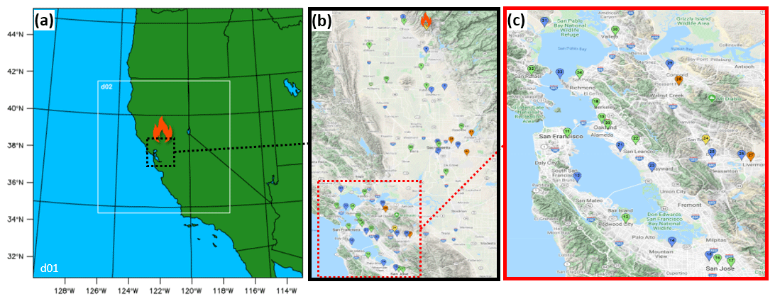
Figure 1Study domain (a) and observation station locations (b, c). Domain d01 covers the western US with a horizontal resolution of 8 km. Domain d02 is centered over Northern California with a horizontal resolution of 2 km. AQS and NCDC observation sites are shown in panels (b) and (c), where stations marked in green measure only PM2.5, stations in blue measure wind and temperature, stations in orange measure both PM2.5 and meteorology, and stations in yellow measure temperature only. Additionally, BC and CO are measured at 8 and 12 sites in the Bay Area, respectively. © Google 2020.
2.1 WRF-Chem configuration
The WRF-Chem simulation time period is 7 November 2018 (a day before the fire began) to 22 November 2018 (when the fire was 90 % contained). We carried out simulations over two domains (Fig. 1): domain d01 includes all of California at 8 km×8 km horizontal resolution, while domain d02 covers Northern California at 2 km×2 km horizontal resolution. A total of 49 vertical layers are used from the surface to 100 hPa with 50 m vertical resolution in the planetary boundary layer. The meteorological boundary and initial conditions for the outer domain are generated from the fifth generation of European Centre for Medium-range Weather Forecasts (ECMWF) reanalysis dataset (ERA5) at 30 km×30 km resolution (Copernicus Climate Change Service, 2017). Chemical boundary and initial conditions for the outer domain are generated from the Model for Ozone and Related Chemical Tracers version 4 (MOZART-4).
We use physical options of the Noah Land-Surface Model (Tewari et al., 2004), the Mellor–Yamada–Janjic (MYJ) boundary layer scheme (Janjic, 1994), and the Rapid Radiative Transfer Model (RRTM) (longwave) and Dudhia (shortwave) radiative transfer schemes (Dudhia, 1989). Cumulus parameterization is not included. The second-generation Regional Acid Deposition Model (RADM2) chemical mechanism coupled with the Modal Aerosol Dynamics model for Europe (MADE) and Secondary Organic Aerosol Model (SORGAM) (Zhao et al., 2011) are employed. Aerosol optical properties are calculated based on the volume approximation, for which the volume average of each aerosol species is used to calculate refractive indices (Jin et al., 2015). Aerosol radiative feedbacks on meteorology and chemistry are included in the simulations.
We use the National Emission Inventory for anthropogenic emissions (US EPA, 2018). Biogenic emissions are calculated online using the Guenther scheme (Guenther et al., 2006). Dust emissions are calculated online using the Goddard Chemistry Aerosol Radiation and Transport (GOCART) dust emission scheme with University of Cologne (UOC) modifications (Shao et al., 2011). Sea salt emissions are excluded. Technical details of wildfire emissions and the plume rise calculation are discussed in the next section.
2.2 Fire emissions inventory and plume rise model
Wildfire emissions are generated using the PREP-CHEM-SRC v1.5 preprocessor (Freitas et al., 2011) employing 3BEM (Longo et al., 2010) with satellite data on detected fires. For each pixel with fire detected, the mass of emitted species is calculated by
for a certain species η, where αveg is the carbon density (the mass of burnable aboveground biomass per unit area of vegetation), βveg is the combustion factor, EFveg is the emission factor by species and vegetation type, and afire is the burning area of each fire pixel. Vegetation type is generated from the MODIS data following the International Geosphere-Biosphere Programme (IGBP) land cover classification. Vegetation-type-specific emission factors (EFveg) and combustion factors (βveg) are derived from Ward et al. (1992) and Andreae and Merlet (2001). Vegetation-type-specific carbon density (αveg) is based on Olson et al. (2000) and Houghton et al. (2001). Active fire detection is retrieved from the VIIRS fire product with 375 m spatial resolution. A limitation of the VIIRS fire count product is its relatively low temporal resolution. As a polar-orbiting satellite, VIIRS provides fire detection during the daytime only once (about 13:30 local time; LT) at each location.
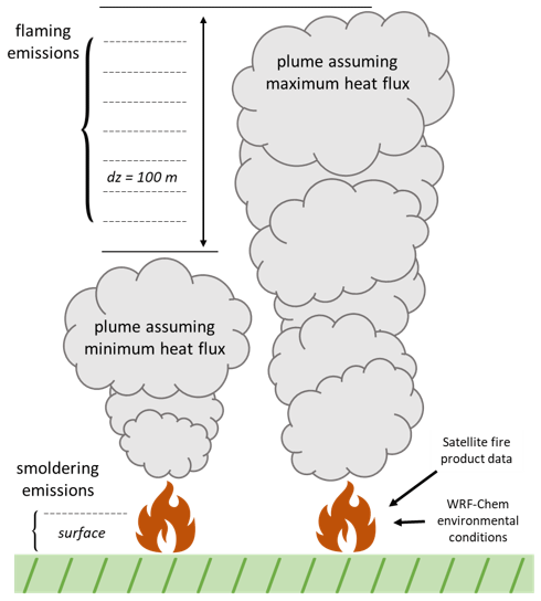
Figure 2Plume rise model schematic. For each grid cell in which wildfire occurs, the plume rise model uses satellite fire products and the surrounding WRF-Chem environmental conditions to calculate two plume-top heights by using the land-type-dependent minimum and maximum wildfire heat fluxes. Smoldering-phase emissions are allotted to the surface layer, while flaming-phase emissions are distributed linearly aloft within the injection layers at a vertical resolution of 100 m.
The emission preprocessor generates a file formatted for WRF-Chem containing the smoldering-phase surface emission fluxes of each species, the fire size for each vegetation type, and flaming factor. Flaming factor is the ratio of biomass consumed in the flaming phase to biomass consumed in the smoldering phase. The 17 IGBP land cover classes are aggregated into four main types: tropical forest, extratropical forest, savanna, and grassland. The size of the wildfire and phase of combustion play important roles in the structure of the plume and the vertical distribution of emissions. Wildfire combustion is generally considered to occur in two phases: smoldering and flaming. Emissions from the smoldering phase are allotted to the first layer of the computational grid, while those from the flaming phase are released at injection heights above the surface, as determined by the plume rise model described below. Fire size determines the total surface heat flux, as well as the entrainment radius of the plume. Fire parameters are ascribed a daily temporal resolution and are distributed to the WRF-Chem domains. The fire parameters are then input to the plume rise model (Freitas et al., 2007, 2010). The plume rise model is a one-dimensional model implemented in each WRF-Chem grid cell with an independent vertical grid resolution of 100 m. It calculates the maximum height to which a plume reaches and distributes emissions therein (Fig. 2). The plume-top height, determined by the surface heat flux from the fire and the thermodynamic stability of the atmospheric environment, is defined as the height at which the in-plume parcel vertical velocity <1 m s−1. The plume rise model uses upper and lower bounds of heat fluxes determined by each land type to calculate the minimum and maximum plume-top height. Flaming emissions are distributed equally to each vertical level within the injection layer with the following calculation: flaming emissions per level are equal to the smoldering emission multiplied by the flaming factor multiplied by DZ−1, where DZ is the minimum plume-top height subtracted from the maximum plume-top height. The model also accounts for entrainment, water balance, and internal gravity wave damping.
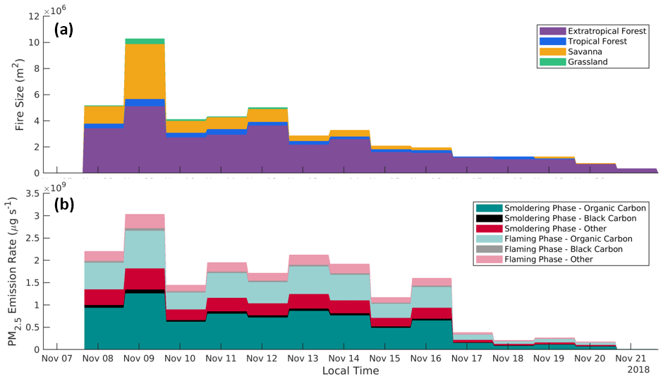
Figure 3Wildfire area by vegetation type in m2 (a) and PM2.5 emission rate in µg s−1 by combustion phase and species (b) input into WRF-Chem. The base inventory is produced from VIIRS and MODIS fire products using the PREP-CHEM-SRC processor and is employed by S_EMRAW. The control and remaining sensitivity simulations use an inventory with triple emission flux of all species on 13 November and double during 13–16 November, shown here. About 59 % of total PM2.5 emissions occur in the smoldering phase (darker colors in panel b). The total PM2.5 emitted is composed of 69.5 % organic carbon and 4.5 % black carbon. The Camp Fire burned primarily extratropical forest (purple) followed by savanna (yellow). Burning of extratropical forest generated the greatest fraction of emissions in the flaming phase at 44.2 %, followed by savanna at 22.9 % and tropical forest at 17.4 %. Grassland emits only in the smoldering phase.
Figure 3 shows the fire size and particulate matter emissions produced from MODIS and VIIRS data. The Camp Fire burned primarily extratropical forest vegetation (which comprised 68 % of the total burned area), followed by savanna (23 % of total area). The flaming emission rate for species n from vegetation type v, is calculated by
At maximum, the carbon monoxide (CO) emission flux was 4.1×10⁷ , and PM2.5 flux was 3.7×10⁴ . On average, 46 % of the fuel burned is estimated to have been consumed during the flaming phase.
The Fire Inventory from NCAR (FINN) version 1.5 (Wiedinmyer, 2011) is another fire emissions product that we will test in a sensitivity analysis. It is assembled for atmospheric chemistry models with a daily temporal resolution and a 1 km horizontal resolution. FINN is generated using satellite observations of active fires and land cover paired with emission factors and fuel loading estimates. The emissions are allocated to a diurnal cycle following WRAP (2005). FINN outputs the total wildfire emission flux, fire size, and land type fraction. As FINN does not include a smoldering- to flaming-phase ratio, the plume rise model calculates a ratio based on CO emissions.
2.3 Surface and satellite observations
The observational data include both ground-based measurements and satellite observations. Meteorological and surface concentration data were obtained from the NOAA's National Climatic Data Center (NCDC) and EPA Air Quality System (AQS), respectively. We focus on three areas: the region closest to the fire, the Sacramento Metro Area (population of 2.5 million), and the San Francisco Bay Area (population of 7 million). Hourly observations of wind speed at 10 m, wind direction at 10 m, temperature at 2 m, PM2.5, black carbon (BC), and CO are available for the sites shown in Fig. 1. We use level-2 products from the TROPOMI aboard the Copernicus Sentinel-5 Precursor (S5P) satellite to evaluate the spatial and vertical distribution of predictions. We compare TROPOMI aerosol layer height retrievals (3.5 km×7 km) with the predicted WRF-Chem height of maximum PM2.5, and ultraviolet aerosol index (UVAI, 3.5 km×7 km) with the predicted WRF-Chem BC columns. The model results are sampled around 13:30 LT when S5P passes over California.
2.4 Control and sensitivity simulations
To investigate the effects of key model parameters on the ability to predict the atmospheric impact of the wildfire, we conduct a range of sensitivity simulations. As meteorology and atmospheric structure play important roles in plume dynamics and the transport of particulate matter, we separately perturb the aerosol radiative feedback to meteorology, the planetary boundary layer parameterization, and the plume entrainment coefficient. To understand further the extent to which fire characteristics provided by satellite data can affect the simulations, we analyze the influence of fire data sources, the emission rate, and partitioning between smoldering-phase and flaming-phase emissions. A summary of these simulations is provided in Table 1.
Table 1Summary of sensitivity simulation setup.
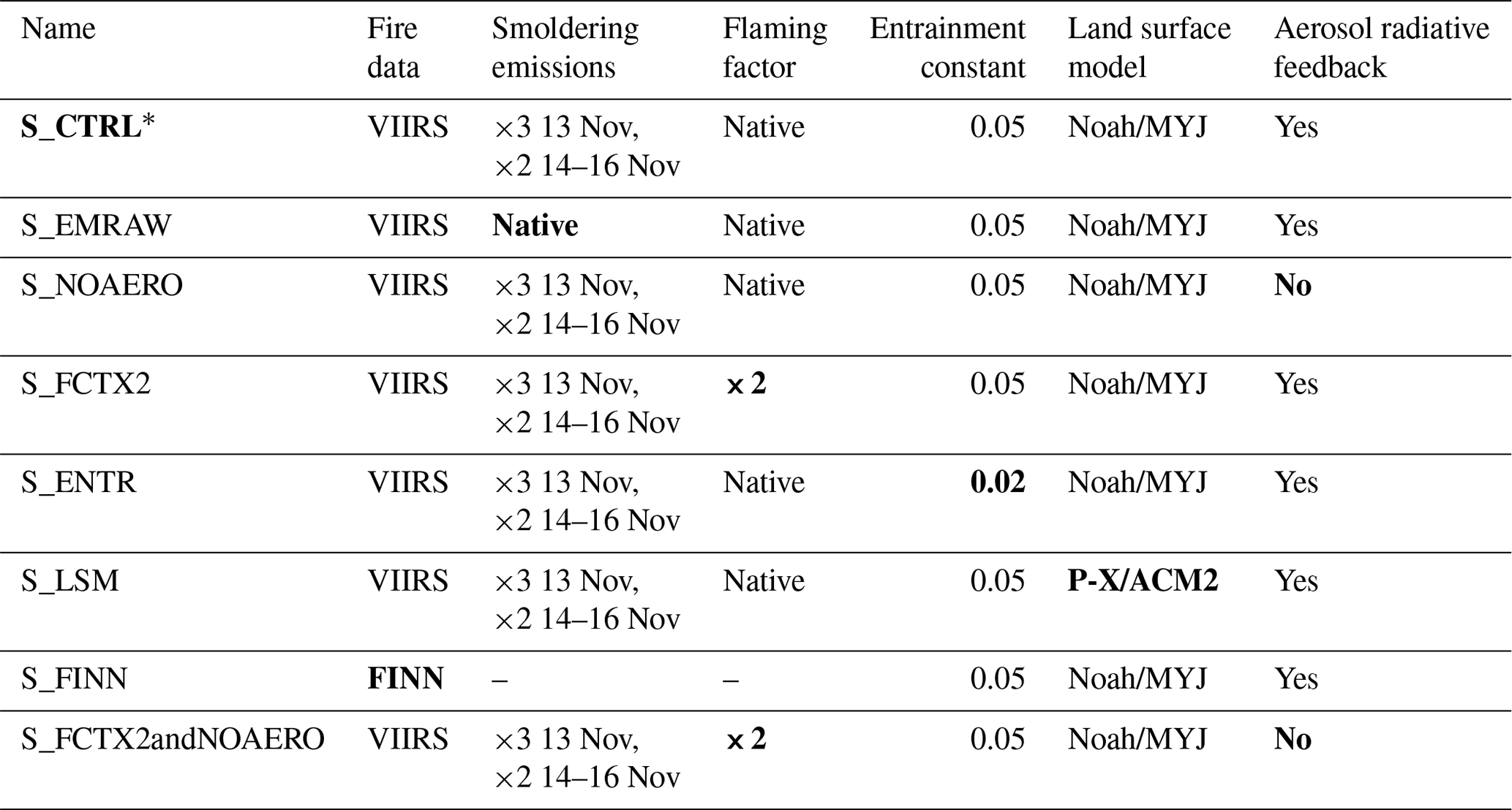
∗ Scenario that agrees best with surface observations and is of primary focus in this study. Bold denotes parameters perturbed from the S_CTRL scenario.
Our evaluation focuses on the control simulation (S_CTRL). S_CTRL applies a factor of 3 to the smoldering emissions on 13 November and a factor of 2 to the smoldering emissions on 14–16 November due to the intermittent cloudy conditions over the Northern California on those days. S_CTRL uses the native flaming factor and fire size products, the default entrainment constant of 0.05, and the MYJ planetary boundary layer scheme. In the following scenarios, one parameter is individually perturbed from this configuration. S_EMRAW uses the native emissions input with unaltered smoldering-phase emissions, S_NOAERO turns off the aerosol radiative feedback to meteorological fields, S_FCTX2 doubles the flaming factor for the entire simulation period (thus increasing flaming-phase emissions without changing the smoldering phase), S_ENTR reduces the entrainment coefficient within the plume rise model from 0.05 to 0.02, and S_LSM employs an alternative land surface model and planetary boundary layer scheme. We perform another sensitivity simulation using FINN in place of VIIRS (S_FINN).
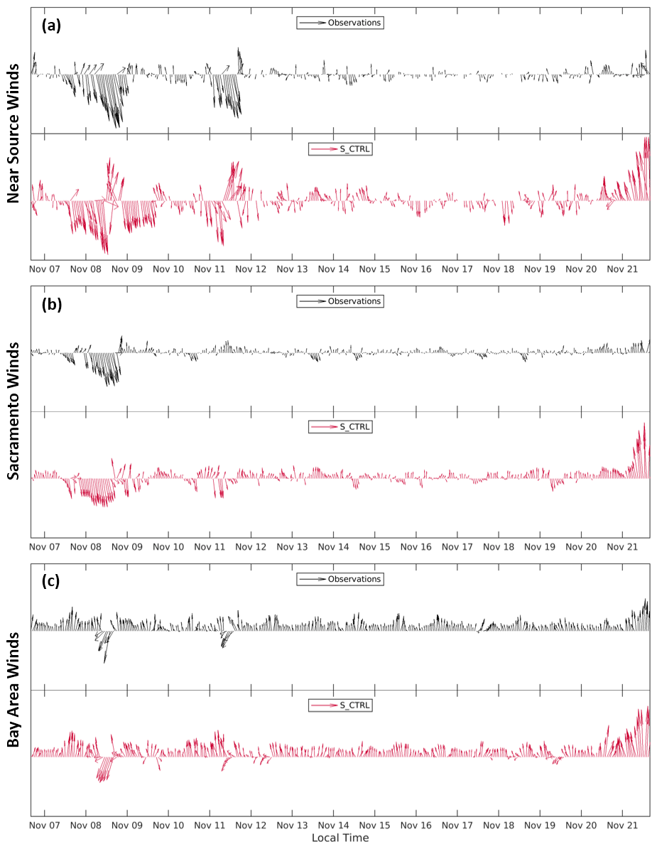
Figure 4Comparison of AQS and NCDC wind observations (black) with S_CTRL predictions (red) averaged over the three areas of study: (a) near the wildfire (N=4), (b) Sacramento (N=6), and (c) the Bay Area (N=12). Arrows indicate the wind direction and their length represents wind speed. For reference, S_CTRL predicts maximum wind speeds of 8.7, 7.5, and 7.1 m s−1 near the source, in Sacramento, and in the Bay Area, respectively. Paradise and the Sacramento areas experienced strong northerly winds during the first few days of the fire. S_CTRL generally predicted faster and more variable winds, but broader trends in Sacramento and the Bay Area were represented well.
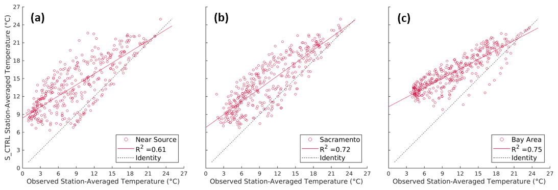
Figure 5Comparison of AQS and NCDC temperature observations versus S_CTRL predictions: (a) near the wildfire (N=10), (b) Sacramento (N=7), and (c) the Bay Area (N=13). The solid red lines show a linear regression fit, while the dotted black lines denote 1:1 simulations versus observations. The simulations achieved a correlation coefficient R2 of 0.61 near the fire, 0.72 in Sacramento, and 0.75 in the Bay Area.
3.1 Meteorology
The three spatial areas of our interest differ significantly in topography and meteorology. Figure 4 shows the averaged wind observations and S_CTRL predictions. S_CTRL captures general wind patterns and achieves strong correlation with observed temperatures in each of the areas (Fig. 5). In the first few days of the Camp Fire, the foothills and the Sacramento area experienced strong northerly winds, while the Bay Area experienced northeasterly winds, both predicted by the simulation. Other distinct features like those on 11 November near the fire and in the Bay Area are also reproduced by S_CTRL with some bias in timing. In the Bay Area, winds were typically southerly at speeds less than 2 m s−1 and consistent through most of the simulation duration. In the relatively dry Sacramento Valley inland, winds were also predominantly southerly but were calmer (<1 m s−1) and varied more than those on the coast. After 11 November, the wind speeds were much slower. Coastal air regulates Bay Area temperatures, whereas the drier Sacramento area experiences a greater temperature range. S_CTRL also produced these relative characteristics but, in general, generated faster winds and higher temperatures than those observed. A summary of model performance statistics is provided in Table 2. The complex terrain of the Bay Area and the Sierra Nevada foothills near the fire location likely contribute to uncertainty in predicting meteorological parameters. Note that the 4–5 K mean biases in the regional surface temperature (T) are non-negligible. Figure 5 shows that the largest biases mainly occur during the night when the hourly temperature reaches the minimum during the day (deviation from the 1:1 line), while the daytime temperature matches relatively well with the observations (close to the 1:1 line). However, it is important to realize that the nighttime temperature biases have little influence on the PM simulations we focus on. The temporal evolutions of observed PM near Sacramento and the Bay Area do not show a clear diurnal cycle (Fig. 6), nor do the modeled PM biases, as shown in the next section.
Table 2Summary of meteorological model performance metrics for the simulation duration.
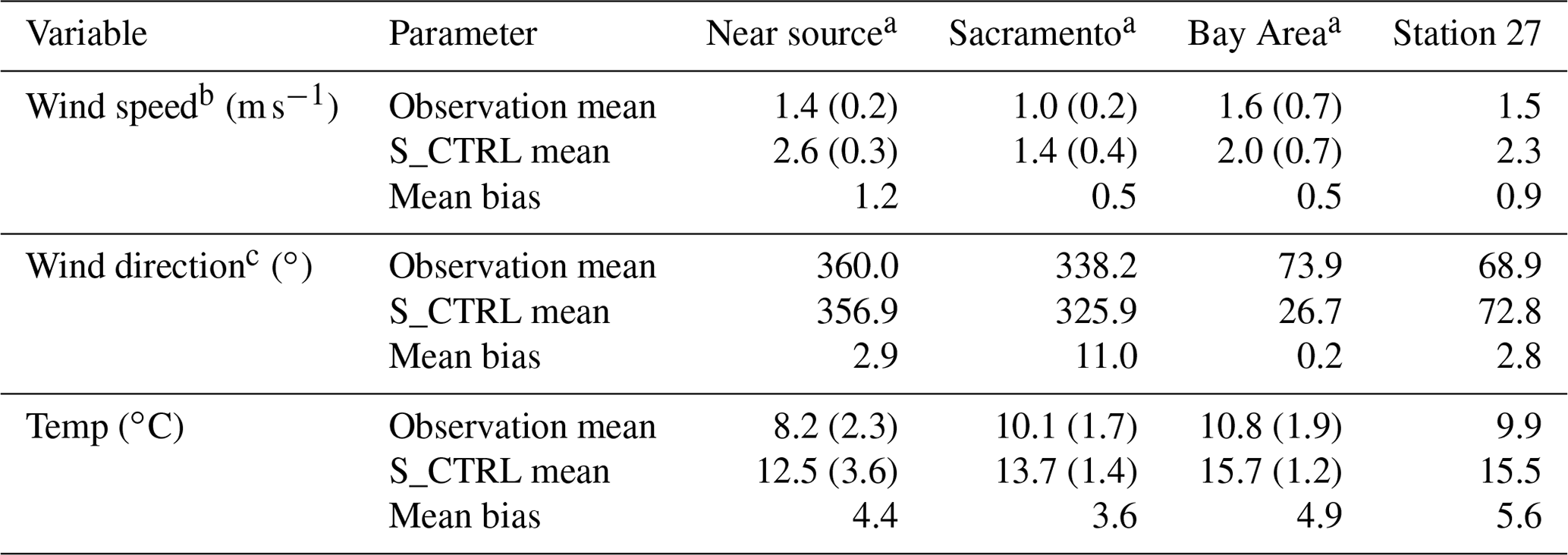
a Area winds are averaged for 4 stations near source, 6 stations in
Sacramento, and 12 stations in the Bay Area. Area temperatures are averaged
for 10 stations near source, 7 in Sacramento, and 13 in the Bay Area.
Standard deviation of station averages is noted in parentheses.
b Mean wind speed is calculated as the average of the magnitude of the
wind vector.
c Mean wind direction is calculated assuming a unity vector.
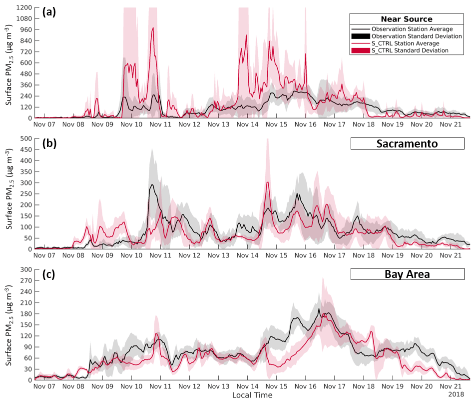
Figure 6Comparison of AQS surface PM2.5 observations (black) with S_CTRL predictions (red) averaged over the three areas of study: (a) near the wildfire (N=5), (b) Sacramento (N=7), and (c) the Bay Area (N=13). Shading indicates the standard deviation of the sampled stations. S_CTRL overpredicted PM2.5 in the region in the vicinity of the fire but performed well in the areas downwind.
3.2 Surface-level particulate matter
Figure 6 shows the predicted evolution of surface PM2.5 from AQS observations and S_CTRL over the period of the wildfire. Within hours of the onset of the Camp Fire, observed PM2.5 concentrations in Sacramento and the San Francisco Bay Area (130 and 240 km downwind) increased from below the National Ambient Air Quality Standard (NAAQS) 24 h average of 35 to 50 µg m−3. Both areas remained above the standard for more than a week, reaching values of 3 times the standard for multiple days. The region near the fire, Sacramento, and the San Francisco Bay Area were each out of attainment of the NAAQS 24 h average of PM2.5 for 11, 11, and 12 d, respectively, during 7–20 November, while S_CTRL predicted 12, 11, and 11 d, respectively. Much of Northern California did not return to attainment until 22 November when the wildfire reached 90 % containment. Table 3 summarizes the ability of S_CTRL to reproduce observed values of surface PM2.5 in the three focus areas and at Stations 27 and 28 in the Bay Area. The model prediction exhibits a mean bias of 64.8 µg m−3 in the region of the Camp Fire, −11.4 µg m−3 in Sacramento, and −16.8 µg m−3 in the Bay Area. Mean bias was smaller at some individual monitoring stations, such as Stations 27 and 28, which have a mean bias of −9.9 and −6.2 µg m−3, respectively. In the broader area near the fire, S_CTRL significantly overestimates surface PM2.5, reaching nearly 1 mg m−3, while observed concentrations peaked closer to 300 µg m−3. However, S_CTRL shows a similar temporal trend to that observed, capturing many peak times. The Sacramento area experienced maxima near 300 µg m−3, while the Bay Area reached around 200 µg m−3. S_CTRL shows good agreement of the magnitude and temporal evolution of surface PM2.5 in the Bay Area and Sacramento for most days, with the exception of 10 November and 14–16 November (to be discussed subsequently). Time series of observed and predicted surface CO and BC in the Bay Area are shown in Fig. 7. Again, S_CTRL shows good agreement with the magnitude and trend of both species. While PM2.5 is largely underpredicted in the period of 14–16 November, BC is overpredicted by 5–10 µg m−3 at peaks. S_CTRL also produces positive bias in surface CO over 16–18 November.
Table 3Summary of model performance metrics for surface PM2.5 (µg m−3) for the simulation duration.
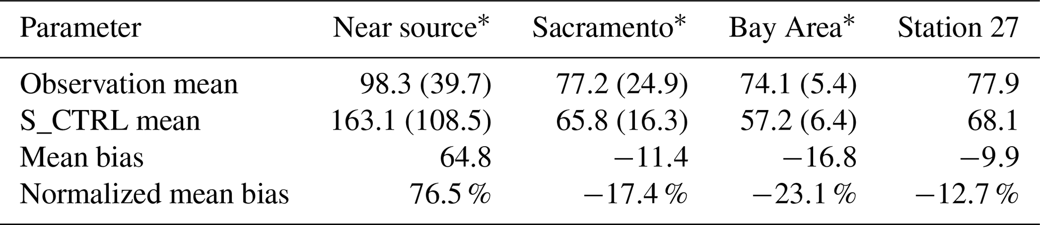
∗ Area values are averaged for 5 stations near source, 7 stations in Sacramento, and 13 stations in the Bay Area. Standard deviation of station averages is noted in parentheses.
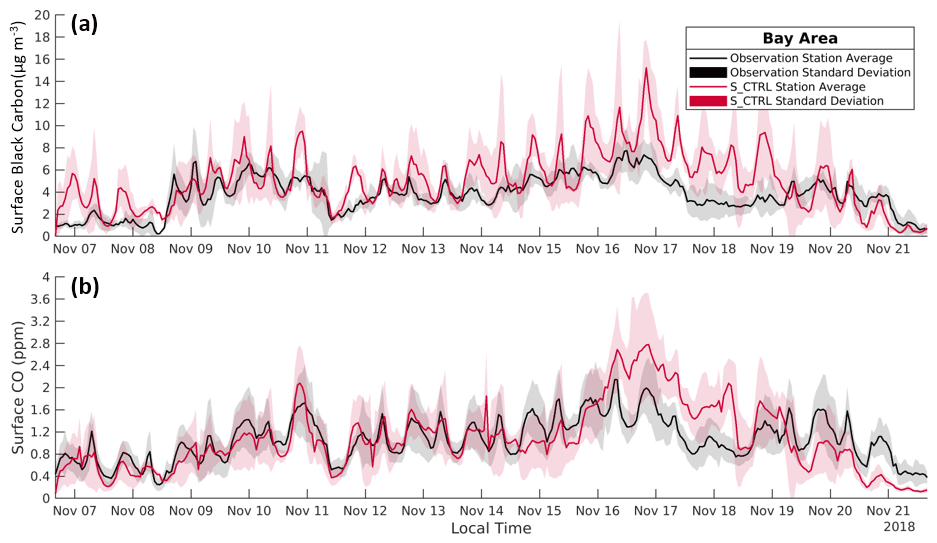
Figure 7Comparison of AQS surface black carbon (a, N=5) and carbon monoxide (b, N=12) observations (black) with S_CTRL predictions (red) at monitoring sites in the Bay Area. S_CTRL captures the temporal evolution of BC and CO and is close to observed values. BC peaks are often overpredicted. The greatest bias of BC and CO occurs during 16–18 November, likely due to the scale factor applied to emissions during 13–16 November.
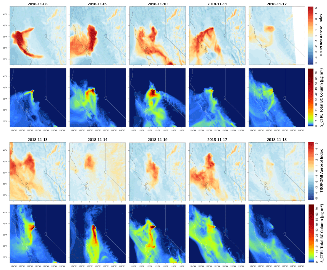
Figure 8Comparison of TROPOMI UV aerosol index and S_CTRL total BC column during 8–18 November at 13:30 LT as a proxy for plume structure and motion. Due to cloud coverage, no data for 15 November are shown. Positive aerosol index (warm colors) indicates aerosols that absorb radiation like black and brown carbon. The spatial distribution of the plume is generally captured on most days. The simulation also captures some of the finer structures seen by the satellite, though they are somewhat displaced.
Error in surface PM2.5 can, in part, be attributed to error in the predicted wind fields. In the latter hours of 8 November near the Camp Fire, S_CTRL predicts southerly winds, while observations are steadily northerly, leading to some return of initially transported plume. Again, on 11 November, predicted winds show a dramatic reversal, and surface PM2.5 spikes. In Sacramento on 10 November, observed and predicted northerly winds at midday initially lead to increased PM2.5 concentrations, but winds swing southerly in the later hours. On 13 November, observed winds blow south and transport emissions to Sacramento, while S_CTRL predicts winds in the opposing direction, leading to an underprediction in PM2.5. However, error in predicted wind fields does not explain the substantial underprediction of surface PM2.5 in the Bay Area over 14–16 November, as the station-averaged winds of the area do not show significant deviation from observations. We tested the four-dimensional data assimilation (FDDA) of large-scale horizontal wind from ERA5, but it could not reduce the aforementioned biases in wind, possibly due to the fact that the observed wind patterns are driven by some mesoscale or even local-scale dynamics.
To study the structural evolution of the wildfire plume, we compare simulated total black carbon column with TROPOMI UVAI satellite retrievals (Fig. 8). TROPOMI UVAI is based on the difference between wavelength-dependent Rayleigh scattering observed in an atmosphere with aerosols and that of a modeled molecular atmosphere (Stein Zweers et al., 2018). This difference is measured in the UV spectral range where ozone absorption is small. A positive residual (red coloring) indicates the presence of UV-absorbing aerosols, like black carbon (BC), while a negative residual (blue coloring) indicates presence of non-absorbing aerosols. As WRF-Chem does not generate an aerosol index parameter, we compare UVAI to total BC column, a significantly absorbing aerosol. Over the period of the simulation, broad characteristics and shape, as well as some more distinct features, of the Camp Fire plume are reproduced by S_CTRL. Using similar input data sources and WRF-Chem configuration but a simpler plume rise model, Shi et al. (2019) also capture the general shape of the plume but underestimate aerosol magnitude. Discrepancies in S_CTRL plume transport correlate to bias in surface PM2.5. On the first day of the fire, observations show that strong winds in Northern California drag the plume west, where steady coastal winds transported the plume south and inland again (Fig. 8). The dynamics creates a dense plume with two narrow stretches. S_CTRL predictions of total BC column fail to capture the hook shape present in the UVAI retrievals but reflect the two separate stretches of narrow plume. The simulation constrains one stretch to the valley, leading to overprediction of surface PM2.5 in Sacramento on 8 November (Fig. 6b). On 11 November, the simulation does not reproduce the second band of the plume which wraps along the coast and towards San Francisco; rather, the plume remains more concentrated to the Sacramento Valley again. This leads to underprediction of surface PM2.5 in the Bay Area and overprediction in Sacramento (Fig. 6b and c). The narrow PM2.5 peaks of S_CTRL on 14–16 November in Sacramento can likely be attributed to the more pronounced plume on 14 and 16 November. A stark horizontal gradient of fire emissions could restrict accumulation of PM2.5 averaged over the Sacramento region.

Figure 9Vertical profile of PM2.5 (a), time series of surface PM2.5 (b), and winds (c; observations in black and predictions in red) at Station 27 in the Bay Area. The gray box highlights the time frame of greatest model bias of surface PM2.5. Sharp increases in PM2.5 correlate with a switch to northeasterly winds that import fire emissions to the Bay Area. A large negative PM2.5 bias on 15 November occurs when S_CTRL deviates from observations and produces southerly winds which bring in clean air. This can be seen in the column of low-level PM on 15 November in panel (a).
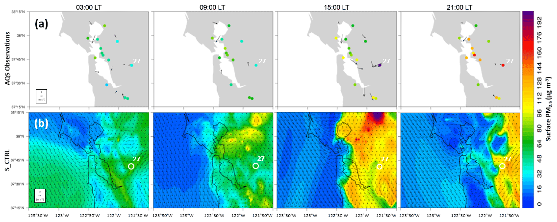
Figure 10Surface PM2.5 and wind field of observations (a) and S_CTRL predictions (b) on 14 November in the Bay Area. Note that the reference wind vector for S_CTRL is 2 m s−1, while the reference is 1 m s−1 for observations. While the plume encroaches on the Bay Area, a strong sea breeze develops midday, driving plumes back inland. This sea breeze is not present in observational data, leading to a large underprediction of surface PM2.5.
To investigate the predicted decrease of surface PM2.5 in the Bay Area on the afternoon of 14 November, we individually analyze Station 27 (Fig. 9). Figure 9 shows the vertical profile of S_CTRL PM2.5 concentrations, the observed and predicted surface PM2.5, and the observed and predicted wind fields. Additionally, Fig. 10 shows the spatial distribution of PM2.5 and surface winds of observations (Fig. 10a) and predictions (Fig. 10b) at four times on 14 November. In the late morning at Station 27, observed winds become northeasterly and PM2.5 spikes as more particle-laden air flows westward (Fig. 9). At the same time, S_CTRL winds also become northeasterly and PM2.5 increases accordingly. However, predicted winds reverse, and PM2.5 levels remain relatively low from midday 14 November to midday 15 November. This behavior emerges as part of a larger flow pattern in Fig. 10. Throughout the morning of 14 November, the simulated wildfire plume approaches the Bay Area and is then driven back inland by a strong sea breeze in the afternoon, not present in the observational data. This behavior is demonstrated in the vertical profile of PM2.5 (Fig. 9a). A column of clean air flushing the Bay Area leads to a predicted bias of −50 µg m−3 on 15 November.
3.3 Aerosol vertical profile
The TROPOMI aerosol layer height (ALH) retrieval represents vertically localized aerosol layers within the free troposphere in cloud-free conditions and is designed to capture aerosol layers produced by biomass burning aerosol (such as wildfires), volcanic ash, and desert dust (Apituley et al., 2018). ALH is retrieved based on the significant effect of aerosol vertical structure on the high-spectral-resolution observations in the O2 A band in the near-infrared spectrum (759 to 770 nm). The ALH algorithm includes a spectral fit estimation of reflectance across the O2 A band using the optimal estimation retrieval method with primary fit parameters of aerosol layer middle pressure and aerosol optical thickness (de Graaf et al., 2019). The assumed aerosol profile is a single uniform scattering layer with a fixed pressure thickness, constant aerosol volume extinction coefficient, and constant aerosol single scatter albedo. The middle pressure of the layer, defined as the average of the top and bottom pressures, is converted to altitude with a temperature profile. This parameterization is best suited for aerosol profiles dominated by a sole elevated and optically thick aerosol layer, which is characteristic of wildfire plumes.
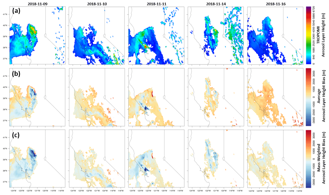
Figure 11Comparison of TROPOMI aerosol layer height (a) and bias where S_CTRL layer height is calculated as the average of heights where PM2.5>3 µg m−3 (b) and the average weighted by PM2.5 mass (c) for select days at 13:30 LT. In panels (b) and (c), warm colors indicate positive bias where S_CTRL overpredicts the height of the aerosol layer.
We compare the satellite-derived aerosol layer height to WRF-Chem predictions of PM2.5 using two methods. We define the smoke aerosol layer with a PM2.5 threshold concentration of 3 µg m−3. For the first method, the layer height is calculated as the average of heights at which PM2.5 is greater than the threshold. For the second method, these heights are weighted by BC mass. Figure 11 shows the satellite-derived layer height (Fig. 11a) and the S_CTRL model bias of average heights (Fig. 11b) and mass-weighted average heights (Fig. 11c). TROPOMI layer heights are generally 1 to 2 km and reach higher than 6 km in some instances. Using purely averaged heights, S_CTRL typically overpredicts ALH by 100 to 400 m and remains within a smaller range than TROPOMI. S_CTRL layer heights weighted by BC mass are lower, thus improving agreement with the satellite. Note that the reported retrieval bias in TROPOMI ALH is about 780 m for wildfire emission plumes and 1.75 km over land generally (Nanda et al., 2020), so the above model–satellite differences in ALH are within the uncertainty range. Archer-Nicholls et al. (2015) and Sessions et al. (2011) also reported overpredicted aerosol layer heights using WRF-Chem when compared to airborne data and Multi-angle Imaging SpectroRadiometer (MISR) stereo heights, respectively. Using CMAQ, however, Herron-Thorpe et al. (2014) reported underpredicted heights when compared to Cloud-Aerosol Lidar with Orthogonal Polarization (CALIOP) products. Archer-Nicholls et al. (2015) found that error in plume injection height can contribute to error in surface PM, and that PM biases were dependent on vegetation type as carbon density and heat release vary by vegetation. Location of the aerosol layer within the column likely also contributes to error in surface predictions of PM2.5 in this study; however, the current analysis is inconclusive. The assumption of a single, elevated aerosol layer used in the TROPOMI ALH derivation may not be characteristic of the vertical structure predicted by WRF-Chem. As seen in Figs. 9 and 10 and in the vertical profile near the wildfire, layers of aerosol are commonly present at the surface and exist as multiple non-localized layers. Sessions et al. (2011) also found that using the FLAMBE fire data preprocessor with emission injection heights not constrained to the boundary layer resulted in better agreement with satellite products than PREP-CHEM-SRC. Consideration of the WRF vertical grid is also necessary when comparing surface level values. Further development of the analytic method used to evaluate WRF-Chem aerosol layer heights may provide insight into the behavior of the plume rise model and its vertical structure.
We conduct sensitivity simulations to investigate the effects of various parameters on the ability of the WRF-Chem model to accurately predict downwind PM concentrations from wildfires. As meteorological conditions and related boundary structure play important roles in plume dynamics and the transport of PM, we separately test the aerosol feedback to meteorology and the land surface model. To understand the extent to which fire characteristics provided by satellite data can affect the simulation, we analyze the fire product sources (VIIRS versus FINN), the total fire emissions, and the division between smoldering-phase and flaming-phase emissions. To examine the influence of the plume rise model, we perturb a key parameter: the entrainment coefficient.
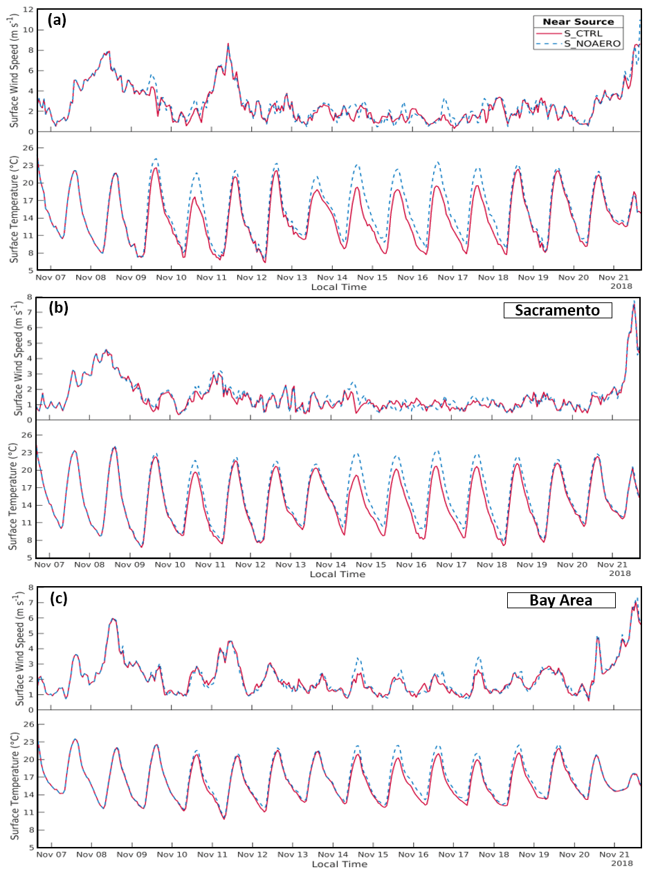
Figure 12Comparison of meteorology generated by S_CTRL (solid red line) and S_NOAERO (in which aerosol effects do not feed back to the meteorology; dashed blue line) over the three areas of study: (a) near the wildfire, (b) Sacramento, and (c) the San Francisco Bay Area. Exclusion of the aerosol feedback has the greatest effect nearest the fire, where S_NOAERO increased wind and temperature by 9.8 % and 9.7 %, respectively, on average. The aerosol feedback mechanism has the least significance in the Bay Area, where S_NOAERO wind speed differs less than 2 % and temperature differs 3.1 % on average. The most pronounced changes occur during 14–16 November when S_CTRL significantly underpredicts surface PM2.5. In WRF-Chem, the feedback of aerosol–radiation interactions on meteorology acts to stabilize the atmosphere, slow wind speeds, and increase PM concentrations.
4.1 Aerosol radiative feedback to meteorology
By absorbing and scattering solar radiation, aerosols can impact the radiative fluxes, cloud formation, and precipitation in the atmosphere (Wang et al., 2016, 2020), and, in turn, the meteorological conditions for aerosol formation, transport, and removal (Li et al., 2019). WRF-Chem has the option to couple aerosol–radiative direct effects with meteorology simulation. S_NOAERO uses the same input data and configuration as S_CTRL but disables the aerosol radiative feedback. Figure 12 shows the evolution of surface wind speed and temperature throughout the wildfire near the source (Fig. 12a), in Sacramento (Fig. 12b), and in the Bay Area (Fig. 12c). The aerosol radiative impact on simulated meteorology is more pronounced for surface temperature than wind. When aerosol radiative feedbacks are noticeable, colder temperatures and calmer winds are found near the surface. Generally, feedbacks are more evident in the region closer to the fire sources with larger PM concentrations. Also, in the Bay Area, the largest changes in meteorology coincide with the largest differences in surface PM2.5 between the two scenarios (Fig. 13), which occurs when higher concentrations are predicted (10–11 November, 14–16 November). Consequently, the aerosol radiative feedback in WRF-Chem acts to stabilize the atmosphere, presumably due to the solar absorption by smoke aerosols and reduction of radiation reaching the surface (Wang et al., 2013). When taking the entire time period into account, the overall smoke radiative effect on meteorology is relatively small in the downwind region, like the Bay Area, even when aerosol concentrations are high.

Figure 13Time series of surface PM2.5 (µg m−3) predicted by the sensitivity simulations (Table 1) averaged for the three areas of study: (a) near the wildfire (N=5), (b) Sacramento (N=7), and (c) the Bay Area (N=13). S_ENTR is omitted from the figure as it resulted in less than 1 % change from S_CTRL. In the Bay Area, S_FCTX2 generally predicted more surface PM2.5, recovering 10–35 µg m−3 on 14–16 November when S_CTRL significantly underpredicted PM2.5 compared to observations. S_EMRAW demonstrates the impact of increasing the emissions inventory for 13–16 November. In the Bay Area, using the unperturbed emissions inventory reduces PM2.5 by more than 30 % over 14–16 November. The impact of the aerosol feedback mechanism on PM2.5 (S_NOAERO) is location dependent. Excluding the feedback to meteorology generally reduces PM2.5 near the wildfire and in the Bay Area, while increasing PM2.5 in Sacramento. Employing the ACM2 PBL scheme results in a vastly different temporal evolution with a distinct diurnal pattern (S_LSM). FINN input fire data produce very little PM2.5.
4.2 Fire emission inventory
Currently, fire emission inventories generally have large uncertainty. Although wildfires have been studied for decades and there is vast literature characterizing biomass combustion emissions, there are large knowledge gaps in the composition of these emissions when a nontrivial fraction of the burnt area includes built environment comprising a vast array of non-biomass-related materials. For the Camp Fire, there is a paucity of the types of burned land cover and fire emissions data required to incorporate these considerations into model simulations. WRF-Chem input fire files produced with VIIRS and PREP-CHEM-SRC include fire size, smoldering emission flux, and flaming factor. Here, we test the sensitivity of predictions to different emission dataset (FINN (S_FINN) versus VIIRS/MODIS), as well as emission injection parameters, such as the smoldering emission flux (S_EMRAW) and flaming factor (S_FCTX2). S_FINN produces very little aerosol, though it captures the timing of some peaks. The aerosol underestimation may be a result of bias in the emission inventory or an issue of its implementation in the plume rise model code, as FINN specifies total wildfire emissions rather than a smoldering and flaming distribution.
When the VIIRS emission inventory is used, the total wildfire emission flux can be altered through two parameters: the smoldering emission flux at the surface and the flaming factor. Directly increasing the smoldering emission flux adds emissions to the surface layer and increases flaming-phase emissions proportionally. Figure 13 shows the impact of doubling smoldering emissions on 13 November and tripling them during 14–16 November. These changes to the inventory more than double concentrations of surface PM2.5 in the area of the wildfire and increase concentrations in the Bay Area by 20 to 60 µg m−3 during 14–16 November. Consequently, increasing input of total wildfire emissions improves the agreement of predictions with observations in Sacramento and the Bay Area, suggesting that some uncertainty may stem from satellite fire products. This finding is supported by Archer-Nicholls et al. (2015), as they applied a factor of 5 to scale up the wildfire emissions in their simulations. By modifying the flaming factor, we perturb only the emissions injected aloft by the plume, as emissions higher in the atmosphere may allow for greater transport downwind. By doubling the flaming factor over the full simulation duration, S_FCTX2 recovers 10–35 µg m−3 in the Bay Area 14–16 November (Fig. 13c), when S_CTRL substantially underpredicts PM2.5.
4.3 Plume rise parameterization – entrainment coefficient
The plume rise model parameterizes entrainment as proportional to the plume vertical velocity and inversely proportional to the plume radius (Freitas et al., 2010). Greater entrainment causes rapid cooling, such that near-surface plume temperatures are only slightly warmer than the environment, lowering buoyancy and reducing the plume height. Larger wildfires generate less entrainment and reach higher injection heights. The parameterization also includes the effect of horizontal winds on entrainment. Strong wind shear can enhance entrainment and increase boundary layer mixing (Freitas et al., 2010). Archer-Nicholls et al. (2015) decreased the original entrainment coefficient (Freitas et al., 2007) from 0.1 to 0.05 to improve their simulations of a wildfire. As the Camp Fire developed rapidly and intensely, we performed the sensitivity simulation S_ENTR with a lower entrainment coefficient of 0.02 to allow for higher injection heights. However, entrainment perturbation resulted in less than 1 % change in surface PM2.5 from S_CTRL. A possible reason is that the background winds were quite strong already, for which the entrainment coefficient played a limited role.
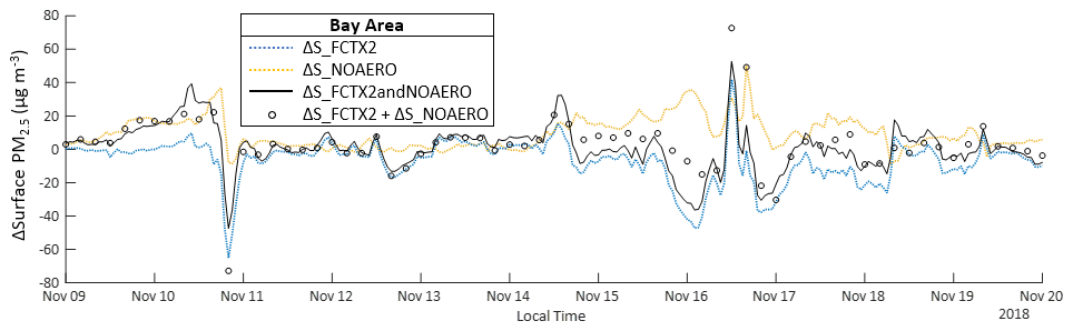
Figure 14Comparison of surface PM2.5 (µg m−3) predicted by the joint perturbation experiment S_FCTX2andNOAERO with individual perturbation experiments (Table 1). ΔS_* is the difference between each perturbation experiment (S_FCTX2 in dotted blue, S_NOAERO in dotted yellow, S_FCTX2andNOAERO in solid black) and the control experiment (S_CTRL). Black circles plot the sum of the effects from S_FCTX2 and S_NOAERO. Generally, the impact of the joint perturbation is similar to the sum of the two individual effects.
We compare simulations using two different land surface models (LSMs) which include the planetary boundary layer (PBL) schemes: the Noah LSM with MYJ PBL and the Pleim–Xiu LSM (referred to here as P-X) with the Asymmetric Convection Model 2 (ACM2) PBL (Janjic, 1994; Pleim and Xiu, 1995; Chen and Dudhia, 2001; Pleim, 2007). Land surface models simulate the heat and radiative fluxes between the ground and the atmosphere (Campbell et al., 2018). The Noah LSM has four soil moisture and temperature layers, while the P-X LSM has two (Hu et al., 2014; Campbell et al., 2018). Both include a vegetation canopy model and vegetative evapotranspiration. The PBL scheme provides the boundary layer fluxes (heat, moisture, and momentum) and the vertical diffusion within the column. It uses boundary layer eddy fluxes to distribute surface fluxes and grows the PBL by entrainment. A key feature of PBL schemes is the inclusion of local mixing (between adjacent layers) and/or non-local mixing (from the surface layer to higher layers). The MYJ scheme is a turbulent kinetic energy prediction, while the ACM2 scheme is a member of the diagnostic non-local class. MYJ solves for the total kinetic energy in each column from buoyancy and shear production, dissipation, and vertical mixing. ACM2 has two main components: a term for local transport by small eddies and a term for non-local transport by large eddies. Coniglio et al. (2013) showed that the MYJ scheme can undermix the PBL in locations upstream of convection in the presence of overly cool and moist conditions near the ground in the daytime, whereas ACM2 can result in an excessively deep PBL in evening. Pleim (AMS, 2007) also noted that ACM2 predicts the PBL profile of potential temperature and velocity with greater accuracy.
The use of P-X and ACM2 results in substantially different aerosol trends and plume evolution, the effects of which are largely location-dependent (Fig. 13). Near the fire and in the Bay Area, S_LSM produces little similarity in surface PM2.5 magnitude and trend as compared to S_CTRL. S_LSM reduces PM2.5 concentrations by more than 50 % in both areas for the majority of the simulation period. However, S_CTRL overpredicts PM2.5 near the wildfire, while S_LSM underpredicts but produces a more muted temporal pattern, similar to observations. In the Sacramento area, S_LSM generally predicts higher PM2.5 values with a distinct diurnal trend. Peaks are of similar magnitude to S_CTRL but displaced temporally. The topography of the Sacramento area is more uniform than the complex terrain of the Bay area as well as the foothills and canyons near the wildfire, likely contributing to the distinctions in the behavior of the two schemes. Moreover, the current sensitivity study stresses the importance of the parameterization of the land surface and the boundary layer. As shown here, the Noah LSM and MYJ scheme perform well for the broader region of Northern California, whereas improvement near the wildfire itself may be attained with altered PBL parameterization.
4.4 Joint perturbation
To test the linearity of different factors in regulating the fire-related PM pollution, we choose two factors, emission flaming factor and aerosol radiative feedback, and conduct a new experiment by jointly perturbing these two. We compare the results from this joint perturbing experiment with those from each individual perturbing experiment and the linear sum of the two in Fig. 14. It shows that for the most times, the effect of joint perturbation is close to the sum of the two individual effects (the black line follows well with the black circles), indicating that the relatively good linearity and additivity hold between those two factors in a general sense. The exception occurs under the extreme conditions. During 14–18 November when the plume was thick and PM2.5 concentration was highest in the Bay Area, the aerosol radiative feedback dominates, and the effect of joint perturbation is close to the aerosol radiative effect (the black line follows well with the dotted blue line).
The record-breaking Camp Fire ravaged Northern California for nearly 2 weeks. At a distance of 240 km downwind of the wildfire, Bay Area surface PM2.5 levels reached nearly 200 µg m−3 and remained over 70 µg m−3 over 7–22 November 2018. It is uncertain to what extent the current chemical transport models can reproduce the key features of this historical event. Here, we employ the WRF-Chem model to characterize the spatiotemporal PM concentrations across Northern California and to investigate the sensitivity of predictions to key parameters of the model. The model utilizes satellite fire detection products with a resolution of 375 m and a biomass burning model to generate the fire emission inventory in near-real time. We conduct model simulations at 2 km resolution. A wide range of observational data is employed to evaluate the model performance, including ground-based observations of PM2.5, black carbon, and meteorology from EPA and NOAA stations, as well as satellite measurements, such as TROPOMI aerosol layer height and aerosol index.
We focus on three geographic areas: the vicinity of the wildfire, Sacramento, and the San Francisco Bay Area. The control experiment was able to simulate the general transport and extent of the plume as well as the magnitude and temporal evolution of surface PM2.5 in Sacramento and the Bay Area. Meanwhile, the control experiment substantially overpredicted surface PM2.5 near the fire but captured the general evolution of the fire development. On the Pacific coast, the Bay Area was subject to significant sea breezes not observed during the time period of simulation. Due to strong winds predicted from the ocean, a large negative bias existed in surface PM2.5. Increasing total wildfire emissions (smoldering and flaming) and increasing flaming-phase emissions alone each recovered some PM2.5 biases. Aerosol radiative feedback on meteorology acted to stabilize the atmosphere and slightly increased the PM2.5 concentration near the surface during most severe episodes. Hence, its inclusion modestly improves model performance. Our study shows that sources of downwind PM error stem primarily from the localized structure of the plume and uncertainty in fire emissions. Uncertainty of partitioning between smoldering and flaming phases may also contribute to uncertainty in plume horizontal transport.
Future studies are needed to further improve the present modeling framework to simulate wildfires. Some wildfires exhibit a distinct diurnal cycle, but the current fire preparation module has not utilized the time information of the fire radiative power measurements by the polar-orbiting satellites. Also, the current land cover and vegetation type data are still relatively coarse in spatial resolution and classification accuracy, which cannot fully resolve a small town in a rural area. In fact, the Camp Fire reportedly burned the town of Paradise, California, between 8 and 10 November 2018. The town of Paradise covered 47 km2 which corresponds to about 7.6 % of the total burned area. This contributes to the uncertainty in the fire emission preparation. Additional verification of input fire data sources, such as FINN, and their implementation in the WRF-Chem plume rise model is needed for studies of the vertical structure. Deeper understanding of the role of plume dynamics and boundary layer parameterization on aerosol concentrations downwind from wildfires will inform updates to forecast models like WRF-SFIRE-CHEM, which couples WRF with a fire spread model and smoke dispersion simulation (Barbuzano, 2019; Kochanski et al., 2013). Given the complexity of the problem, we only perturb individual factors in this study. Future studies can test different combinations of the main factors identified by the present study, which can yield additional insights about non-linear interactions among different processes related to fire emission and transport.
The recent TROPOMI aerosol layer height product shows promise as an analytical tool but requires further development of the method by which it can be directly compared to WRF-Chem. Given the assumptions required to perform the TROPOMI ALH retrieval, more research is needed to compare that product with any height retrievals from MODIS/MAIAC (Lyapustin et al. 2020), MISR, and CALIPSO. The intercomparison can help quantify measurement uncertainty. Herron-Thorpe et al. (2014) noted that careful consideration must also be given to the vertical coordinates across models and satellite products, as discrepancies in reporting heights in reference to sea level, ground level, or the geoid can influence analyses.
WRF-Chem model code is available for download via the WRF website (https://www2.mmm.ucar.edu/wrf/users/downloads.html, last access: June 2018).
US Environmental Protection Agency Air Quality System Data Mart (internet database) is available for download (https://www.epa.gov/airdata, last access: June 2019). NCDC data are available for download via the NCEI website (https://www.ncei.noaa.gov/metadata/geoportal/rest/metadata/item/gov.noaa.ncdc:C00684/html#, last access: June 2019). TROPOMI data are available for download via the Copernicus Open Access Hub website (https://scihub.copernicus.eu/, last access: October 2019). ERA5 data are available for download via the Copernicus Climate Data Store website (https://cds.climate.copernicus.eu/, last access: March 2019). FINN emission data are available for download via the NCAR Atmospheric Chemistry Observations and Modeling website (http://bai.acom.ucar.edu/Data/fire, last access: January 2020).
YW, JHS, and JHJ conceived and designed the research. YW and BR performed the WRF-Chem simulations. BR, YW, and JHS performed the data analyses and produced the figures. BZ provided technical support for fire emission preparation. ZCZ helped satellite data analyses. BR, YW, and JHS wrote the paper. All authors contributed to the scientific discussions and preparation of the manuscript.
The authors declare that they have no conflict of interest.
This study was supported by the Jet Propulsion Laboratory, California Institute of Technology, under contract with NASA. We thank Kristal R. Verhulst, Yi Yin, Don Longo, Gonzalo Ferrada, and Saulo Freitas for their support and discussion.
This study has been supported by the AQ-SRTD project at the Jet Propulsion Laboratory, California Institute of Technology, under contract with NASA, and the NASA ACMAP, CCST, and TASNPP programs.
This paper was edited by Joshua Fu and reviewed by two anonymous referees.
Andreae, M. O. and Merlet, P.: Emission of trace gases and aerosols from biomass burning, Global Biogeochem. Cycles, 15, 955–966, https://doi.org/10.1029/2000GB001382, 2001.
Apituley, A., Pedergnana, M., Sneep, M., Pepijn Veefkind, J., Loyola, D., Landgraf, J., and Borsdorff, T.: Sentinel-5 precursor/TROPOMI Level 2 Product User Manual Carbon Monoxide, SRON-S5P-LEV2-MA-002, available at: http://www.tropomi.eu/sites/default/files/files/Sentinel-5P-Level-2-Product-User-Manual-Carbon-Monoxide_v1.00.02_20180613.pdf (last access: October 2019), 2018.
Archer-Nicholls, S., Lowe, D., Darbyshire, E., Morgan, W. T., Bela, M. M., Pereira, G., Trembath, J., Kaiser, J. W., Longo, K. M., Freitas, S. R., Coe, H., and McFiggans, G.: Characterising Brazilian biomass burning emissions using WRF-Chem with MOSAIC sectional aerosol, Geosci. Model Dev., 8, 549–577, https://doi.org/10.5194/gmd-8-549-2015, 2015.
Barbuzano, J.: Wildfire smoke traps itself in valleys, Eos, 100, https://doi.org/10.1029/2019EO135955, 2019.
Brown, T., Leach, S., Wachter, B., and Gardunio, B.: The Northern California 2018 Extreme Fire Season, in: Explaining Extremes of 2018 from a Climate Perspective, B. Am. Meteorol. Soc., 101, S1–S4, https://doi.org/10.1175/BAMS-D-19-0275.1, 2020.
Campbell, P. C., Bash, J. O., and Spero, T. L.: Updates to the Noah land surface model in WRF-CMAQ to improve simulated meteorology, air quality, and deposition, J. Adv. Model. Earth Syst., 11, 231–256, https://doi.org/10.1029/2018MS001422, 2018.
Cascio, W. E.: Wildland fire smoke and human health, Sci. Total Environ., 624, 586–595, https://doi.org/10.1016/j.scitotenv.2017.12.086, 2018.
Chen, F. and Dudhia, J.: Coupling an advanced land surface-hydrology model with the Penn State-NCAR MM5 modeling system, part I, model implementation and sensitivity, Mon. Weather Rev., 129, 586–585, 2001.
Coniglio, M. C., Correia, J., Marsh, P. T., and Kong, F.: Verificationof Convection-Allowing WRF Model Forecasts of the PlanetaryBoundary Layer Using Sounding Observations, Weather Forecast., 28, 842–862, https://doi.org/10.1175/WAF-D-12-00103.1, 2013.
Copernicus Climate Change Service: ERA5: Fifth generation of ECMWF atmospheric reanalyses of the global climate, Copernicus Climate Change Service Climate Data Store (CDS), available at: https://cds.climate.copernicus.eu/cdsapp#!/home (last access: 22 May 2020), 2017.
De Graaf, M., de Haan, J. F., and Sanders, A. F. J.: TROPOMI ATBD of the Aerosol Layer Height, S5P-KNMI-L2-0006-RP, available at: http://www.tropomi.eu/sites/default/files/files/publicSentinel-5P-TROPOMI-ATBD-Aerosol-Height.pdf (last access: January 2020), 2019.
Dudhia, J.: Numerical study of convection observed during the Winter Monsoon Experiment using a mesoscale two-dimensional model, J. Atmos. Sci., 46, 3077–3107, https://doi.org/10.1175/1520-0469(1989)046<3077:NSOCOD>2.0.CO;2, 1989.
Emmons, L. K., Walters, S., Hess, P. G., Lamarque, J.-F., Pfister, G. G., Fillmore, D., Granier, C., Guenther, A., Kinnison, D., Laepple, T., Orlando, J., Tie, X., Tyndall, G., Wiedinmyer, C., Baughcum, S. L., and Kloster, S.: Description and evaluation of the Model for Ozone and Related chemical Tracers, version 4 (MOZART-4), Geosci. Model Dev., 3, 43–67, https://doi.org/10.5194/gmd-3-43-2010, 2010.
Freitas, S. R., Longo, K. M., Chatfield, R., Latham, D., Silva Dias, M. A. F., Andreae, M. O., Prins, E., Santos, J. C., Gielow, R., and Carvalho Jr., J. A.: Including the sub-grid scale plume rise of vegetation fires in low resolution atmospheric transport models, Atmos. Chem. Phys., 7, 3385–3398, https://doi.org/10.5194/acp-7-3385-2007, 2007.
Freitas, S. R., Longo, K. M., Trentmann, J., and Latham, D.: Technical Note: Sensitivity of 1-D smoke plume rise models to the inclusion of environmental wind drag, Atmos. Chem. Phys., 10, 585–594, https://doi.org/10.5194/acp-10-585-2010, 2010.
Freitas, S. R., Longo, K. M., Alonso, M. F., Pirre, M., Marecal, V., Grell, G., Stockler, R., Mello, R. F., and Sánchez Gácita, M.: PREP-CHEM-SRC – 1.0: a preprocessor of trace gas and aerosol emission fields for regional and global atmospheric chemistry models, Geosci. Model Dev., 4, 419–433, https://doi.org/10.5194/gmd-4-419-2011, 2011.
Guenther, A., Karl, T., Harley, P., Wiedinmyer, C., Palmer, P. I., and Geron, C.: Estimates of global terrestrial isoprene emissions using MEGAN (Model of Emissions of Gases and Aerosols from Nature), Atmos. Chem. Phys., 6, 3181–3210, https://doi.org/10.5194/acp-6-3181-2006, 2006.
Herron-Thorpe, F. L., Mount, G. H., Emmons, L. K., Lamb, B. K., Jaffe, D. A., Wigder, N. L., Chung, S. H., Zhang, R., Woelfle, M. D., and Vaughan, J. K.: Air quality simulations of wildfires in the Pacific Northwest evaluated with surface and satellite observations during the summers of 2007 and 2008, Atmos. Chem. Phys., 14, 12533–12551, https://doi.org/10.5194/acp-14-12533-2014, 2014.
Houghton, R., Lawrence, K., Hackler, J., and Brown, S.: The spatial distribution of forest biomass in the Brazilian Amazon: A comparison of estimates, Global Change Biol., 7, 731–746, https://doi.org/10.1046/j.1365-2486.2001.00426.x, 2001.
Hu, Z., Zhong-Feng, X., Ning-Feng, Z., Ma, Z., and Guo-Ping, L.: Evaluation of the WRF model with different land surface schemes: a drought event simulation in southwest China during 2009–10, Atmos. Ocean. Sc. Lett., 7, 168–173, https://doi.org/10.3878/j.issn.1674-2834.13.0079, 2014.
Janjic, Z. I.: The Step–Mountain Eta Coordinate Model: Further developments of the convection, viscous sublayer, and turbulence closure schemes, Mon. Weather Rev., 122, 927–945, https://doi.org/10.1175/1520-0493(1994)122<0927:TSMECM>2.0.CO;2, 1994.
Jin, Q., Wei, J., Yang, Z.-L., Pu, B., and Huang, J.: Consistent response of Indian summer monsoon to Middle East dust in observations and simulations, Atmos. Chem. Phys., 15, 9897–9915, https://doi.org/10.5194/acp-15-9897-2015, 2015.
Kahn, R.: A global perspective on wildfires, Eos, 101, https://doi.org/10.1029/2020EO138260, 2020.
Kochanski, A., Beezley, D., Mandel, J., and Clements, B.: Air pollution forecasting by coupled atmosphere-fire model WRF and SFIRE with WRF-Chem, ArXiv: 1304.7703 [physics.ao-ph], 2013.
Li, Z., Wang, Y., Guo, J., Zhao, C., Cribb, M. C., Dong, X., Fan, J., Gong, D., Huang, J., Jiang, M., Jiang, Y., Lee, S.-S., Li, H., Li, J., Liu, J., Qian, Y., Rosenfeld, D., Shan, S., Sun, Y., Wang, H., Xin, J., Yan, X., Yang, X., Yang, X., Zhang, F., and Zheng, Y.: East Asian Study of Tropospheric Aerosols and Impact on Regional Cloud, Precipitation, and Climate (EAST-AIRCPC), J. Geophys. Res., 124, 13026–13054, 2019.
Longo, K. M., Freitas, S. R., Andreae, M. O., Setzer, A., Prins, E., and Artaxo, P.: The Coupled Aerosol and Tracer Transport model to the Brazilian developments on the Regional Atmospheric Modeling System (CATT-BRAMS) – Part 2: Model sensitivity to the biomass burning inventories, Atmos. Chem. Phys., 10, 5785–5795, https://doi.org/10.5194/acp-10-5785-2010, 2010.
Lyapustin, A., Wang, Y., Korkin, S., Kahn, R., and Winker, D.: MAIAC Thermal Technique for Smoke Injection Height From MODIS, IEEE Geosci Remote Sens. Lett., 7, 730–734, 2020.
Nanda, S., de Graaf, M., Veefkind, J. P., Sneep, M., ter Linden, M., Sun, J., and Levelt, P. F.: A first comparison of TROPOMI aerosol layer height (ALH) to CALIOP data, Atmos. Meas. Tech., 13, 3043–3059, https://doi.org/10.5194/amt-13-3043-2020, 2020.
Olson, J., Watts, J., and Allison, L.: Major world ecosystem complexes ranked by carbon in live vegetation: A database, Oak Ridge National Laboratory, Oak Ridge, Tennessee, USA, 2000.
Pimlott, K., Laird, J., and Brown, E. G.: 2015 Wildfire Activity Statistics, California Department of Forestry and Fire Protection, available at: https://www.fire.ca.gov/media/10061/2015_redbook_final.pdf (last access: January 2019), 2016.
Pleim, J. E.: A Combined Local and Nonlocal Closure Model for the Atmospheric Boundary Layer. Part I: Model Description and Testing, J. Appl. Meteor. Climatol., 46, 1383–1395, https://doi.org/10.1175/JAM2539.1, 2007.
Pleim, J. and Xiu, A.: Development and testing of a surface flux and planetary boundary layer model for application in mesoscale models, J. Appl. Meteorol., 34, 16–34, https://doi.org/10.1175/1520-0450-34.1.16, 1995.
Schneising, O., Buchwitz, M., Reuter, M., Bovensmann, H., and Burrows, J. P.: Severe Californian wildfires in November 2018 observed from space: the carbon monoxide perspective, Atmos. Chem. Phys., 20, 3317–3332, https://doi.org/10.5194/acp-20-3317-2020, 2020.
Sessions, W. R., Fuelberg, H. E., Kahn, R. A., and Winker, D. M.: An investigation of methods for injecting emissions from boreal wildfires using WRF-Chem during ARCTAS, Atmos. Chem. Phys., 11, 5719–5744, https://doi.org/10.5194/acp-11-5719-2011, 2011.
Shao, Y., Ishizuka, M., Mikami, M., and Leys, J.: Parameterization of size-resolved dust emission and validation with measurements, J. Geophys. Res.-Atmos., 116, D08203, https://doi.org/10.1029/2010JD014527, 2011.
Shi, H., Jiang, Z., Zhao, B., Li, Z., Chen, Y., Gu, Y., Jiang, J. H., Lee, M., Liou, K. N., Neu, J., Payne, V., Su, H., Wang, Y., Marcin, W., and Worden, J.: Modeling study of the air quality impact of record-breaking Southern California wildfires in December 2017, J. Geophys. Res.-Atmos., 124, 6554–6570, https://doi.org/10.1029/2019JD030472, 2019.
Stein Zweers, D.: TROPOMI ATBD of the UV aerosol index, S5P-KNMI-L2-0008-RP, available at: http://www.tropomi.eu/sites/default/files/files/S5P-KNMI-L2-0008-RP-TROPOMI_ATBD_UVAI-1.1.0-20180615_signed.pdf (last access: June 2019), 2018.
Tewari, M., Chen, F., Wang, W., Dudhia, J., LeMone, M. A., Mitchell, K., Ek, M., Gayno, G., Wegiel, J., and Cuenca, R. H.: Implementation and verification of the unified NOAH land surface model in the WRF model, 20th conference on weather analysis and forecasting/16th conference on numerical weather prediction, Seattle, WA, pp. 11–15, January 2004.
US Environmental Protection Agency: National Emissions Inventory (NEI), available at: https://www.epa.gov/air-emissions-inventories/national-emissions-inventory-nei, last access: 5 July 2018.
Wang, Y., Khalizov. A., Levy, M., and Zhang, R.: New Directions: Light Absorbing Aerosols and Their Atmospheric Impacts, Atmos. Environ., 81, 713–715, https://doi.org/10.1016/j.atmosenv.2013.09.034, 2013.
Wang, Y., Ma, P.-L., Jiang, J., Su, H., and Rasch, P.: Towards Reconciling the Influence of Atmospheric Aerosols and Greenhouse Gases on Light Precipitation Changes in Eastern China, J. Geophys. Res.-Atmos., 121, 5878–5887, https://doi.org/10.1002/2016JD024845, 2016.
Wang, Y., Le, T., Chen, G., Yung, Y.L., Su, H., Seinfeld, J. H., and Jiang, J. H.: Reduced European aerosol emissions suppress winter extremes over northern Eurasia, Nat. Clim. Change, 10, 225–230, https://doi.org/10.1038/s41558-020-0693-4, 2020.
Ward, D., Susott, R., Kauffman, J., Babbitt, R., Cummings, D., Dias, B., Holben, B. N., Kaufman, Y. J., Rasmussen, R. A., and Setzer, A. W.: Smoke and fire characteristics for cerrado and deforestation burns in Brazil: BASE-B experiment, J. Geophys. Res., 97, 14601–14619, https://doi.org/10.1029/92JD01218, 1992.
Wiedinmyer, C., Akagi, S. K., Yokelson, R. J., Emmons, L. K., Al-Saadi, J. A., Orlando, J. J., and Soja, A. J.: The Fire INventory from NCAR (FINN): a high resolution global model to estimate the emissions from open burning, Geosci. Model Dev., 4, 625–641, https://doi.org/10.5194/gmd-4-625-2011, 2011.
WRAP (Western Regional Air Partnership): 2002 Fire Emission Inventory for the WRAP Region – Phase II, Project No. 178-6, available at: http://www.wrapair.org/forums/fejf/tasks/FEJFtask7PhaseII.html (last access: January 2019), 2005.
Zhao, C., Liu, X., Ruby Leung, L., and Hagos, S.: Radiative impact of mineral dust on monsoon precipitation variability over West Africa, Atmos. Chem. Phys., 11, 1879–1893, https://doi.org/10.5194/acp-11-1879-2011, 2011.