Microphysical properties of three types of snow clouds: implication for satellite snowfall retrievals

Ground-based radar and radiometer data observed during the 2017–2018 winter season over the Pyeongchang area on the east coast of the Korean Peninsula were used to simultaneously estimate both the cloud liquid water path and snowfall rate for three types of snow clouds: near-surface, shallow, and deep. Surveying all the observed data, it is found that near-surface clouds are the most frequently observed cloud type with an area fraction of over 60 %, while deep clouds contribute the most in snowfall volume with about 50 % of the total. The probability distributions of snowfall rates are clearly different among the three types of clouds, with the vast majority hardly reaching 0.3 mm h⁻¹ (liquid water equivalent snowfall rate) for near-surface, 0.5 mm h⁻¹ for shallow, and 1 mm h⁻¹ for deep clouds. However, the liquid water paths in the three types of clouds all have the substantial probability to reach 500 g m⁻². There is no clear correlation found between snowfall rate and the liquid water path for any of the cloud types. Based on all observed snow profiles, brightness temperatures at Global Precipitation Measurement Microwave Imager (GPM/GMI) channels are simulated, and the ability of a Bayesian algorithm to retrieve snowfall rate is examined using half the profiles as observations and the other half as an a priori database. Under an idealized scenario, i.e., without considering the uncertainties caused by surface emissivity, ice particle size distribution, and particle shape, the study found that the correlation as expressed by R² between the “retrieved” and “observed” snowfall rates is about 0.32, 0.41, and 0.62, respectively, for near-surface, shallow, and deep snow clouds over land surfaces; these numbers basically indicate the upper limits capped by cloud natural variability, to which the retrieval skill of a Bayesian retrieval algorithm can reach. A hypothetical retrieval for the same clouds but over ocean is also studied, and a major improvement in skills is found for near-surface clouds with R² increasing from 0.32 to 0.52, while a smaller improvement is found for shallow and deep clouds. This study provides a general picture of the microphysical characteristics of the different types of snow clouds and points out the associated challenges in retrieving their snowfall rate from passive microwave observations.

1 Introduction

Snowfall is an important component in the global hydrological cycle. Its global distribution may be observed using satellite-based passive and active microwave sensors. Currently, there are multiple satellites in operation carrying passive microwave sensors that are potentially able to be used for snowfall observations, which offers great spatial and temporal coverages for various snowfall-related studies. Meanwhile, while only a few spaceborne active sensors are currently available for snowfall observations, they have the advantage of providing information on the vertical structure of precipitation. Nevertheless, whether active or passive sensors are used, in order to convert the observed radiative signatures (brightness temperature or radar reflectivity) to snowfall rate, two factors related to the snow clouds play an essential role: one is the vertical extent of the cloud layer, and the other is the cloud microphysical properties such as particles' phase and amount. Using ground-based observations from multiple sensors, in this study we intend to understand these properties for three distinctive types of snow clouds. By performing radiative transfer simulations, we further investigate the implication of the variability in microphysical properties to satellite snowfall retrievals from passive microwave observations.

Snowfall retrieval has been investigated recently for both active and passive satellite measurements. The cloud radar on board the CloudSat satellite (Stephens et al., 2002; Tanelli et al., 2008) is the first spaceborne active sensor in operation that is suitable for snowfall observations. It has a minimum detectability of nearly −30 dBZ near the ground, allowing us to observe the weak scattering signal from snowflakes. Kulie et al. (2016) used CloudSat cloud classification and snowfall rate retrievals to partition snowfall observations into shallow cumuliform and deep nimbostratus snowfall categories. Their results show that there are abundant shallow snow cloud cells globally and they can be associated with strong convection and heavy snowfall. For example, they found that shallow snowfall comprises about 36 % of the 2006–2010 CloudSat snowfall dataset by occurrence while constituting some 18 % of the estimated annual global snowfall accumulation. Shallow precipitation can be easily missed by space-borne radars. Although CloudSat radar provides information on the vertical structure of precipitation, there is a blind zone below about 1.5 km due to ground clutter contamination. In most analyses, the lowest range bin (bin depth is ∼240 m) where radar data are not contaminated by surface clutter is often the third (fifth) above the actual surface over oceanic (land) surfaces (Wood et al., 2013; Kulie and Bennartz, 2009; Liu, 2008a; Marchand et al., 2008). Hudak et al. (2008) studied the ability of CloudSat radar to detect precipitation in cold season clouds using data from a C-band weather radar at King City, Ontario, Canada. They found that the most frequent cause of a miss in detection by CloudSat radar was due to ground clutter removal of valid echoes by the algorithm. Similarly, Chen et al. (2016) compared snowfall estimates from CloudSat radar (Wood et al., 2013) and the ground-radar-derived Multi-Radar and Multi-Sensor (MRMS) product (Zhang et al., 2016) and found that the lowest height with valid estimates for most (99.41 %) snowfall events in the CloudSat product is over 1 km above the surface, whereas for 76.41 % of the corresponding MRMS observations, it is below 1 km.

Using satellite passive microwave observations at high-frequency channels, snowfall may be retrieved due to the scattering of upwelling radiation by snowflakes (Katsumata et al., 2000; Bennartz and Bauer, 2003; Skofronick-Jackson and Johnson, 2011; Gong and Wu, 2017). Retrieval algorithms have been developed both in research mode (Kim et al., 2008; Kongoli et al., 2015; Liu and Seo, 2013; Noh et al., 2006; Skofronick-Jackson et al., 2004) and for operations (Kummerow et al., 2015; Meng et al., 2017). Skofronick-Jackson et al. (2004) and Kim et al. (2008) developed physically based retrieval algorithms which seek the best match between radiative transfer model simulated and satellite observed brightness temperatures. The Liu and Seo (2013) and Kongoli et al. (2015) algorithms are mostly statistical, and many pairs of radar and/or gauge-measured snowfall and satellite measured brightness temperatures are used to develop their statistical relations. The Noh et al. (2006) and Kummerow et al. (2015) snowfall algorithms are based on the Bayesian theorem; an a priori database linking snowfall and brightness temperatures needs to be prepared before conducting retrievals. The snowfall rates in a Bayesian algorithm database are often retrievals from radars, and the brightness temperatures are either collocated measurements of passive microwave radiometers or simulated measurements by radiative transfer models. The Meng et al. (2017) algorithm uses a one-dimensional variational method to seek the consistency between measured brightness temperatures and microphysical properties in the atmospheric column. Its performance has been verified by surface radar and gauge observations over the USA with satisfactory results.

Although the above successes have been formerly achieved by investigators, there are still large discrepancies among different snowfall retrievals (Casella et al., 2017; Skofronick-Jackson et al., 2017; Tang et al., 2017). Algorithm uncertainty arises from many factors; one of them is the insufficient knowledge of microphysical properties of the snow clouds and, in particular, the amount of cloud liquid water. The increase in brightness temperature over cloudy skies due to liquid water emission in snow clouds complicates the snowfall detection and retrieval problems (Liu and Curry, 1997; Liu and Seo, 2013; Wang et al., 2013). Wang et al. (2013) showed that the warming by liquid water emission has a similar magnitude to the cooling by ice scattering on microwave brightness temperatures at frequencies higher than 80 GHz. Liu and Seo (2013) discovered a warming rather than cooling signal in high-frequency brightness temperature in most snowfall cases they analyzed.

In addition, correctly simulating brightness temperatures is needed for physical snowfall retrievals, as well as data assimilation of radiance observations in numerical weather prediction models. Yin and Liu (2019) have studied the bias characteristics of observed minus simulated brightness temperatures at high-frequency channels of the Global Precipitation Measurement Microwave Imager (GPM/GMI) under snowfall conditions. In their study, a radiative transfer model that includes single-scattering properties of nonspherical snow particles is used to simulate brightness temperatures at 89 through 183 GHz. The input snow water content profiles are derived from CloudSat radar measurements. The results show that the discrepancy between simulated and observed brightness temperatures is the greatest for very shallow (cloud top around 2 km) or very deep (cloud top around 8 km) snow clouds with discrepancy values being over 10 K in the former and over 30 K in the latter case, although it is generally less than 3 K when averaged over all selected pixels under snowfall conditions. They explained the results as follows. For very shallow snow clouds, cloud liquid water may be rich, and it contributes substantially to the observed brightness temperatures. However, the radiative transfer model, which uses CloudSat radar and GMI retrievals as input, failed to account for this liquid water abundance, resulting in a large discrepancy between simulated and observed brightness temperatures. For very deep snow clouds, they hypothesized that CloudSat radar experiences substantial attenuation, as well as non-Rayleigh scattering, which leads to higher simulated brightness temperatures than observed. A better understanding of the microphysical properties in very shallow and very deep snow clouds is clearly needed to reduce the discrepancies between simulated and observed brightness temperatures.

A field experiment was conducted over the Korean Peninsula during the winter of 2017–2018, coinciding with the 2018 winter Olympic Games (ICE-POP 2018; International Collaborative Experiments for Pyeongchang 2018 Olympic and Paralympic Winter Games). The experiment focuses on the measurement, physics, and improved prediction of heavy orographic snow in the Pyeongchang region of South Korea (Gehring et al., 2020). During the field experiment, many ground-based observations including radar, radiometer, and in situ observations were conducted. In this study, we analyze the vertical structure and microphysical properties of these snow clouds with a focus on their potential impacts on satellite remote sensing of snow precipitation. The main objective of the study is to gain a better understanding of the characteristics of snow clouds that are critical to satellite remote sensing of snowfall. Furthermore, we examine how a Bayesian snowfall retrieval algorithm with GPM/GMI observations would perform for the snow clouds observed during this field experiment.

2 Data and methods

2.1 Ground-based cloud radar and radiometer

Observations from the Radiometer Physics GmbH frequency modulated continuous wave 94 GHz cloud radar (RPG-FMCW, 2015) are the primary data source for this study. This vertical pointing radar is installed at 37.66^∘ N, 128.70^∘ E (altitude 735 m above sea level) over the Korean Peninsula during the ICE-POP 2018 field campaign. It has an operation frequency of 94 GHz for radar backscatter and Doppler spectrum measurements and an embedded 89 GHz passive channel for liquid water path measurements. It is noted that while we refer to this instrument as a cloud radar for convenience, it indeed includes an independent passive microwave channel at 89 GHz which is used for cloud liquid water estimation. There is clearly an advantage of this instrument in studying the composition of cloud liquid water and ice over those that measure radar reflectivity and brightness temperature by two separate instruments because this instrument measures emission and scattering signatures from the same cloud volume and, therefore, avoids the beam mismatching problem of a separated radar and radiometer. The vertical resolution of radar reflectivity measurements is selectable from 1, 5, 10, or 30 m with an overall radar calibration accuracy better than 0.4 dB. The minimum detectable radar reflectivity depends on the range and vertical resolution; at its typical operation mode of 30 m resolution, it is −36 dBZ at 10 km height, which is sufficiently sensitive for snowfall detection. In addition to radar reflectivity, the RPG-FMCW also measures the Doppler spectrum with a Doppler velocity resolution of 1.5 cm s⁻¹. A detailed explanation of the calibration of this instrument can be found in Küchler et al. (2017).

2.2 Retrieved microphysical variables

In this study, the radar reflectivity Z_e is converted to snow water content (SWC) and snowfall rate (S) using the Z_e–SWC relation of Yin and Liu (2017) and Z_e–S relation of Liu (2008a). Before performing these conversions, radar reflectivity was corrected for attenuation due to absorption by atmospheric gases and cloud liquid water and to scattering by ice particles. Absorption by atmospheric gases is calculated based on Rosenkranz (1998) for water vapor and Schwartz (1998) for oxygen with input for geophysical parameters interpolated from the Modern Era Reanalysis for Research and Applications Version 2 (MERRA-2) (Gelaro et al., 2017). Absorption by cloud liquid water is computed using the liquid water path derived by the method described later in this section and assuming cloud liquid water uniformly distributed vertically in the radar echo layer. The refractive index of liquid water is calculated based on Liebe et al. (1993). Attenuation due to ice scattering was readily performed by manufacturer-provided processing software (RPG-FMCW, 2015).

The Yin and Liu (2017) Z_e–SWC relation (SWC in g m⁻³; Z_e in mm⁶ m⁻³) is given by

$$\begin{array}{}\text{(1)}& \mathrm{SWC}=\mathrm{0.024}{Z}_{\mathrm{e}}^{\mathrm{0.75}}.\end{array}$$

In developing the above equation, three snow particle types are employed: sectors, dendrites (Liu, 2008b), and oblate aggregates (Honeyager et al., 2016). The backscatter cross sections of the three snowflake types are computed using discrete dipole approximation (DDA) (Draine and Flatau, 1994; Liu, 2004). It should be mentioned that although Eq. (1) is developed for CloudSat radar, which has the same frequency as the RPG-FMCW radar, uncertainties in particle shapes and size distributions will certainly cause errors in the snow water content derived in this study.

The Liu (2008a) S–Z_e relation is given by

$$\begin{array}{}\text{(2)}& Z_{\mathrm{e}}=\mathrm{11.5}{S}^{\mathrm{1.25}},\end{array}$$

where S is the liquid water equivalent snowfall rate (in mm h⁻¹; Z_e in mm⁶ m⁻³). The backscatter cross sections in Eq. (2) are computed for rosettes, sectors, and dendrites using DDA (Liu, 2008b).

In addition to radar reflectivity, the mean Doppler velocity, and spectral width, the RPG-FMCW also measures brightness temperature at 89 GHz. While there is a liquid water path (LWP) variable produced by the manufacturer-provided software, details about the liquid water path retrieval algorithm and its accuracy have not been well documented. In this study, we chose to adapt the algorithm of Liu and Takeda (1988) in computing the liquid water path from 89 GHz brightness temperatures. Briefly, the brightness temperature T_B received by an uplooking radiometer can be divided into two portions, i.e., the cloud-free atmospheric emission and the liquid cloud water emission. The emissivity of the liquid water cloud ε_c may then be approximated by

$$\begin{array}{}\text{(3)}& {\mathit{\epsilon }}_{\mathrm{c}}={\displaystyle \frac{T_{\mathrm{a}}\left(T_{\mathrm{B}}-T_{\mathrm{Ba}}\right)}{T_{\mathrm{c}}\left(T_{\mathrm{a}}-T_{\mathrm{Ba}}\right)}},\end{array}$$

where T_a is a radiatively mean temperature of the atmosphere in Kelvin, which can be evaluated by absorption-coefficient-weighted averaged atmospheric temperatures in the vertical. Its value roughly equals the temperature at around 1.5 km altitude. T_c is the mean temperature of the cloud layer, which is determined in this study by the air temperature at the height of the geometric middle of valid radar reflectivity profiles. T_Ba is the brightness temperature from the liquid-free atmosphere, which is derived using interpolation between measured T_Bs at echo-free regions in this study. From ε_c calculated with Eq. (3), the liquid water path (LWP) can be derived by

$$\begin{array}{}\text{(4)}& \mathrm{LWP}={\displaystyle \frac{\mathit{\lambda }{\mathit{\rho }}_{\mathrm{L}}}{\mathrm{6}\mathit{\pi }\mathrm{\Im }\left\{\frac{m^{\mathrm{2}}-\mathrm{1}}{m^{\mathrm{2}}+\mathrm{2}}\right\}}}\ln \left(\mathrm{1}-{\mathit{\epsilon }}_{\mathrm{c}}\right),\end{array}$$

where m is the refractive index of water at temperature T_c, λ is wavelength, ρ_L is liquid water density (1000 kg m⁻³), and ℑ{ } indicates the imaginary part. In this study, the refractive index of liquid water is calculated based on Liebe et al. (1993). It should be cautioned that the refractive index at high microwave frequencies may not be very accurate for supercooled liquid water, as pointed out by Kneifel et al. (2014), which can result in errors in the liquid water path estimation. Another error in the liquid water path estimation can be caused by the omission of the reflection from snow particles to the upwelling radiation originating from surface emissions in the retrieval algorithm. Based on the estimation by Kneifel et al. (2010), this reflection can enhance downward radiation by 5 K at 89 GHz where heavy snow clouds occur. The formulation of the current liquid water path retrieval algorithm has the advantage of using cloud-free observations (T_Ba in Eq. 3) as background to calculate cloud emissivity, which is particularly useful when water vapor observations are lacking. However, the drawback is that it cannot include the contribution of ice scattering.

In Fig. 1, an example is shown of the liquid water path retrieved in this study, together with radar reflectivity cross sections and the liquid water path retrieval from the manufacturer-provided algorithm. It can be seen that in cloud-free regions, our liquid water path retrievals are close to zero, while the manufacturer-provided retrievals have a positive bias of about 30 g m⁻². In cloudy regions, the two liquid water path values are more closely comparable to each other. Based on this comparison, we believe that the liquid water path values retrieved in this study are more reasonable. Therefore, our retrievals will be used in the following analysis.

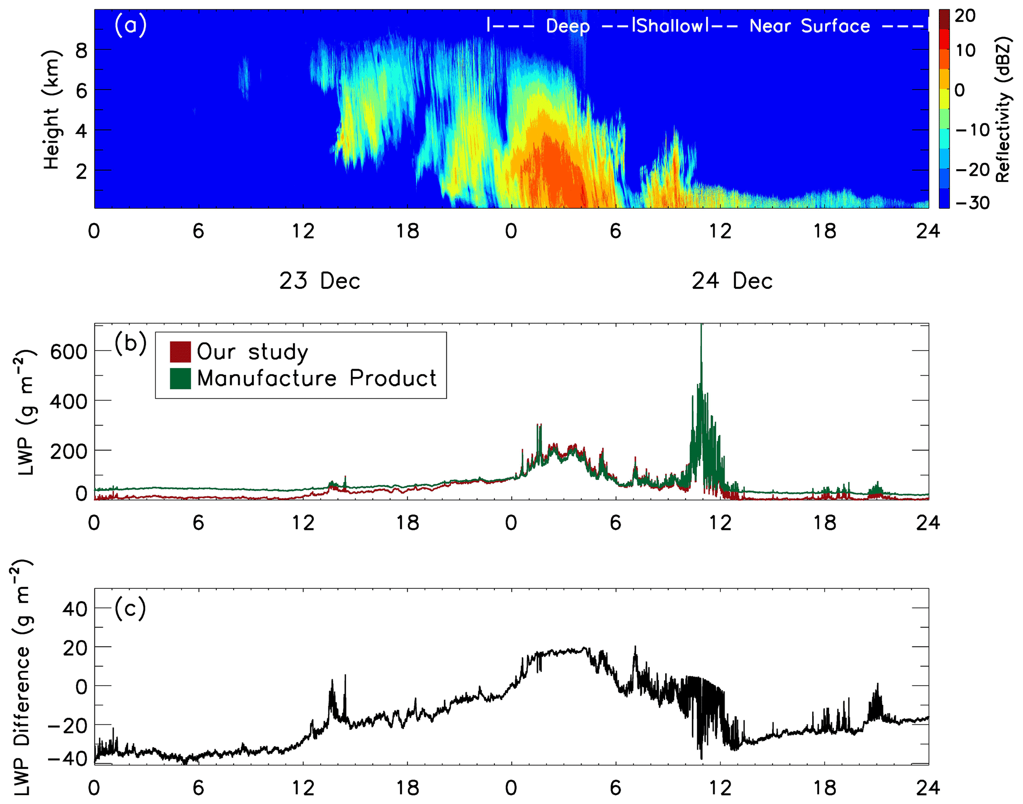
Figure 1 (a) Radar reflectivity, (b) two liquid water path retrievals, and (c) their differences (LWP of our study minus manufacturer's product) for observations during 23 and 24 December 2017. In (a), cloud types as defined in the text are also indicated.

2.3 Snow cloud detection

All snow events have been identified from the RPG-FMCW observations from 1 November 2017 through 30 April 2018 (6 months). To separate snow and rain at the surface level, the scheme of Sims and Liu (2015) is implemented. In their study, the effects of multiple geophysical parameters on the precipitation phase were investigated using global surface-based observations over multiple years. They showed that wet-bulb temperature is a key parameter for separating solid and liquid precipitation, and the low-level temperature lapse rate also affects the precipitation phase. Geophysical parameters from MERRA-2 reanalysis (Gelaro et al., 2017) were used in this study as input for the Sims and Liu (2015) scheme. In addition, we use a near-surface reflectivity higher than −20 dBZ as the criterion for snowfall detection; all radar data analyzed for snow clouds in the following sections have a near-surface radar reflectivity greater than −20 dBZ. In a study by Wang et al. (2017) based on CloudSat radar reflectivity profiles, they found that precipitation onset often occurs when radar reflectivity is about −18 to −13 dBZ. We use the value of −20 dBZ as the criterion in this study to make sure that all possible snowfall cases are included in the precipitation samples.

Cloud top height is used for the determination of cloud types. As shown in Fig. 2, radar reflectivity above cloud top is often noisy, as shown between 11:00 and 16:00 UTC. Therefore, it is often problematic to determine cloud top height by simply using a radar reflectivity threshold. However, we found that Doppler spectral width is a reliable indicator for identifying clouds, as shown in the bottom panel in Fig. 2. Using visual examinations of this and some other cases, we found that Doppler spectral width commonly reduces to less than 0.1 m s⁻¹ above cloud top. In Fig. 2, we show in the upper panel the cloud top height with a solid black line, as determined by the criterion of the spectral width >0.1 m s⁻¹ for snow clouds with near-surface radar reflectivity greater than −20 dBZ. It appears that the criterion captures the cloud tops well.

Figure 2 Height–time cross section of (a) radar reflectivity and (b) Doppler spectral width for observations on 25 November 2017. The cloud top for snow clouds (surface radar reflectivity greater than −20 dBZ) is also shown in (a).

2.4 Other ancillary data

While a quantitative analysis was not conducted, data collected at the same location by a PARticle SIze VELocity (PARSIVEL) disdrometer (Löffler-Mang and Joss, 2000; Battaglia et al., 2010; Tokay et al., 2014), two-dimensional video disdrometer (2DVD; Kruger and Krajewski, 2002), and Multi-Angle Snowflake Camera (MASC; Garrett et al., 2012; Grazioli et al., 2017) are used for confirmation of precipitation phase and particle types. A PARSIVEL is an optical disdrometer which uses a 54 cm² laser beam at a 650 nm wavelength. It measures the size and fall velocity of individual precipitation particles with diameters ranging from 0.2 to 25 mm for solid particles. An autonomous PARSIVEL unit (Chen et al., 2017) from NASA was collocated with the RPG-FMCW cloud radar during the field campaign. A collocated 2DVD provides detailed information on size, fall velocity, and shape of individual hydrometeors with two orthogonal fast line-scan cameras. The camera provides images of particles which are matched for individual particles. The matched individual particles are then corrected for shape distortion. In addition, detailed images of particles are provided from MASC, which is composed of three cameras separated horizontally by an angle of 36 degrees that simultaneously take high-resolution (35 µm per pixel) photographs of free-falling hydrometeors. A hydrometeor classification algorithm based on the supervised machine learning technique (Praz et al., 2017) is applied to the individual images of particles. This procedure identified the precipitation type (small particles, columnar crystals, planer crystals, combination of columnar and plate crystals, aggregates, and graupel) and the degree of riming.

2.5 Dividing snow clouds into three types

There are several synoptic weather patterns that cause snowfall over the Pyeongchang area. The first pattern is a synoptic low-pressure system, a so-called “cold low”, developing over the Yellow Sea (west of Korea) or the cold continent which causes snowfall over the northern and middle part of Korea when moving to the east (Chung et al., 2006; Ko et al., 2016; Park et al., 2019). As this system crosses the Korean Peninsula, the system become weaker and shallower once it moves over the Pyeongchang area. The precipitation intensity and depth of the system depend on the strength of the low pressure. The second synoptic pattern, “warm low”, develops over the warm ocean near East China Sea or South Sea and moves to the northeast or east (Nam et al., 2014; Gehring et al., 2020). This synoptic pattern brings abundant moisture to the Korean Peninsula and is typically favorable for a vertically well-developed precipitation system. As the warm low pressure passes the Korean Peninsula and East sea, the winds over the Pyeongchang area and East China Sea turn easterly or northeasterly, bringing in cold air to the east coastal area. Thus, we expect that the depth of the precipitation system is likely first deep with substantial moisture and later becomes shallower as it is influenced by northeasterly cold air. The third interesting pattern, the so-called “air–sea interaction”, is developed by the easterly or northeasterly flow due to the Kaema high over the northern mountain complex or high pressure over Manchuria by the eastward expansion of the Siberian high (Kim and Jin, 2016; Kim el at., 2019). Thus, the cold northeasterly or easterly flow enhances the interaction with warm moisture ocean, resulting in the development of shallow convection and thermal inversion in the lower troposphere. The shallow convective clouds move to the coastal and mountain areas where they are lifted by the orography.

An example of a radar reflectivity cross section is shown in Fig. 1, in which deeper clouds lead to shallower convective cells. This is the case of the second synoptic type, the warm low. During the passage of the warm low, the system reached to 9 km. However, the precipitation system is shallower than 1 km during easterly or north-easterly flow when the warm low pressure passed the East sea. In consideration of the implications for satellite snowfall remote sensing, we group the snow clouds into three types: deep, shallow, and near surface. The “deep” snow clouds are those with cloud tops higher than 4 km, which are considered to be easily detected by both space-borne radars and radiometers at high microwave frequencies. They are mostly generated by large-scale lifting of frontal systems. We define the “shallow” snow clouds as those with cloud tops between 1.5 and 4 km. A large part of the snow clouds in this group are associated with convective cells in unstable air masses after the passing of fronts. These are the group that space-radars and radiometers may sometimes have difficulties in detecting because of their shallowness and liquid-water richness. The “near-surface” group is defined as those having cloud tops lower than 1.5 km. Similar to the case of shallow snow clouds, the near-surface snow clouds also mostly occur after low pressure passes or during northeasterly/easterly flow, and they are convective in nature. Because of their shallowness, this group of snow clouds will likely be hidden from space-based radars within ground clutters. Ground-based observations have the advantage of detecting them from the bottom up.

In Fig. 1, examples are shown for the three snow cloud types, together with the liquid water path retrieved from RPG-FMCW observations using algorithms described in Sect. 2.2. In this case, the largest value of the liquid water path was seen in the transition from shallow to near-surface snow clouds around 12:00 UTC, while the strongest radar reflectivity values (i.e., the heaviest snowfall) occurred in the deep snow clouds between 01:00 and 05:00 UTC on 24 December 2017.

Surveying all observed data for the entire winter, approximately 374 h of observations are deemed to be snowfall events after we apply the −20 dBZ threshold at the lowest bin and the Sims and Liu (2015) algorithm to exclude rain events. These observations are then averaged over each 5 min interval to form 4491 samples. The relative frequencies of occurrence (area fraction, calculated by the number of samples of a given snow type divided by the total number of snowfall samples) and snowfall amount (volume fraction, calculated by the snowfall amount produced by a given snow type divided by the total snowfall amount by all types) for the three types of snow clouds are shown in Fig. 3. The snowfall volume is the accumulated snowfall with the rate estimated by Eq. (2) from radar reflectivity at the lowest bin. Over half (67.4 %) of the observed samples are near-surface snowfall, followed by shallow (21.2 %) and then deep (11.4 %) snow clouds. However, deep snow clouds contribute the most to the total snowfall volume (45.3 %), followed by shallow (28.5 %) and then near-surface (26.2 %) snow clouds. Pettersen et al. (2020) analyzed snow clouds observed by a micro rain radar at Marquette, Michigan, USA, for four winter seasons. Snow clouds are divided into shallow (top height lower than 1.5 km) and deep events. They found that shallow clouds occur twice as often as deep clouds, while both types contribute almost equally to annual snowfall accumulation. Those statistics are very similar to the results obtained in this study for snowfall events observed at Pyeongchang, Republic of Korea. Kulie et al. (2016) found that globally, shallow snow clouds can be associated with strong convections and heavy snowfall. The snowfall rates for shallow and near-surface snow clouds observed in this study are mostly lower than 0.5 mm h⁻¹; heavy snowfall is mainly associated with deep snow clouds. One possible explanation of the difference is as follows. The snowfall from shallow and near-surface snow clouds in this study mostly comes from convections associated with cold air mass outbreak from the northwest. Since the observation site is in the mountains in the eastern coastal region of the Korean Peninsula, a substantial portion of the moisture picked up by the cold air from the warm ocean in the Yellow Sea (west of the Korean Peninsula) has already been transformed to snow before reaching the observation site. In addition, the convective clouds and easterly flow can cross the mountains and produce heavy snowfall over the site in the case of strong winds and lower thermal stability. However, these types of events occurred relatively infrequently during the experiment when compared to the other snowfall types. Consequently, the snowfall associated with shallow and near-surface clouds at this site is relatively moderate.

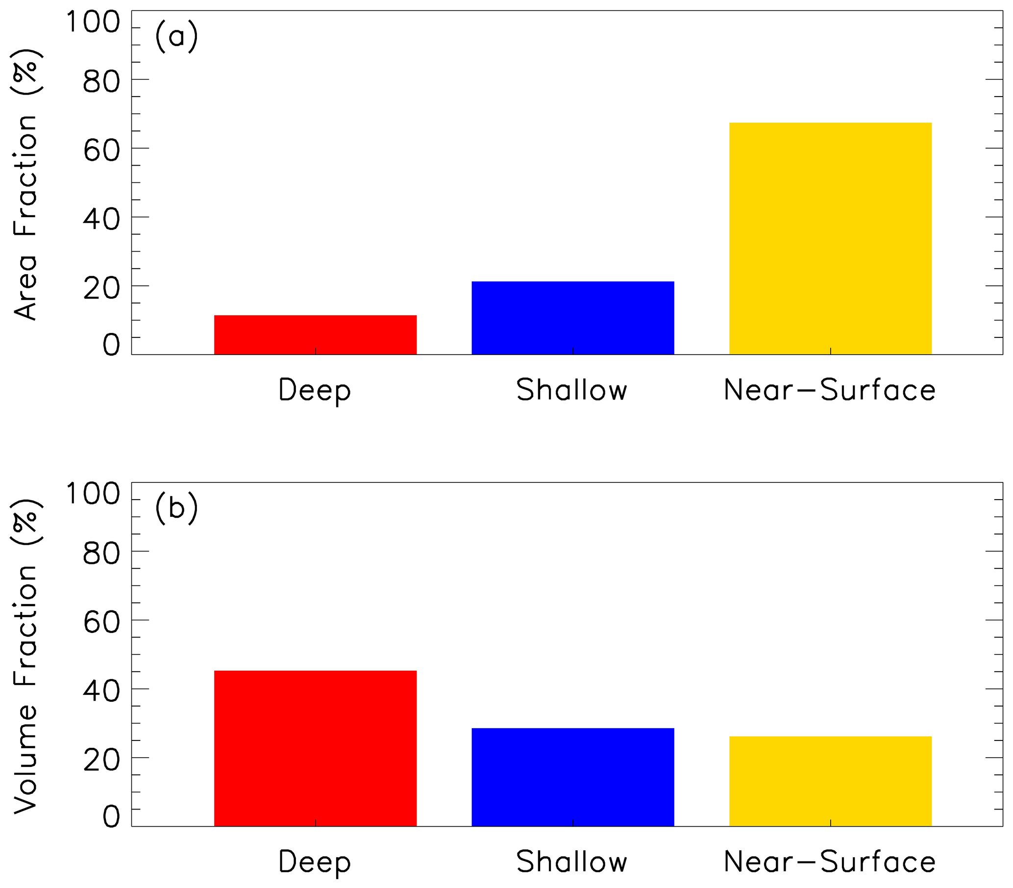
Figure 3 (a) Area and (b) volume fractions of the three types of snow clouds observed during the 2017–2018 winter season.

3 Microphysical properties of snow clouds

3.1 Case examples

3.1.1 Deep and “dry” followed by near-surface snow clouds

From 7 to 8 March 2018, a low-pressure system passed the south of the Korea Peninsula, and solid precipitation was observed at the radar site from 09:00 UTC on the 7th through 24:00 UTC on the 8th. In Fig. 4, cross sections of radar reflectivity and time variation of the liquid water path and snow water path (SWP, vertically integrated snow water content) are shown. Surface PARSIVEL and 2DVD observations indicated that snow particle types were mostly snowflakes from 09:00 UTC on the 7th to 06:00 UTC on the 8th, while rimed ice particles and graupels were also observed thereafter. The radar and radiometer observations indicate that the deep clouds have cloud tops higher than 8 km and a peak snow water path value of about 500 g m⁻². However, liquid water in the deep clouds is low with the liquid water path constantly below 150 g m⁻². Once the deep clouds passed the station, the clouds became much shallower, mostly being classified as near-surface snow clouds. However, their liquid water path increased substantially with peak values close to 600 g m⁻², which is consistent with the observed rimed ice particles and graupels during this period.

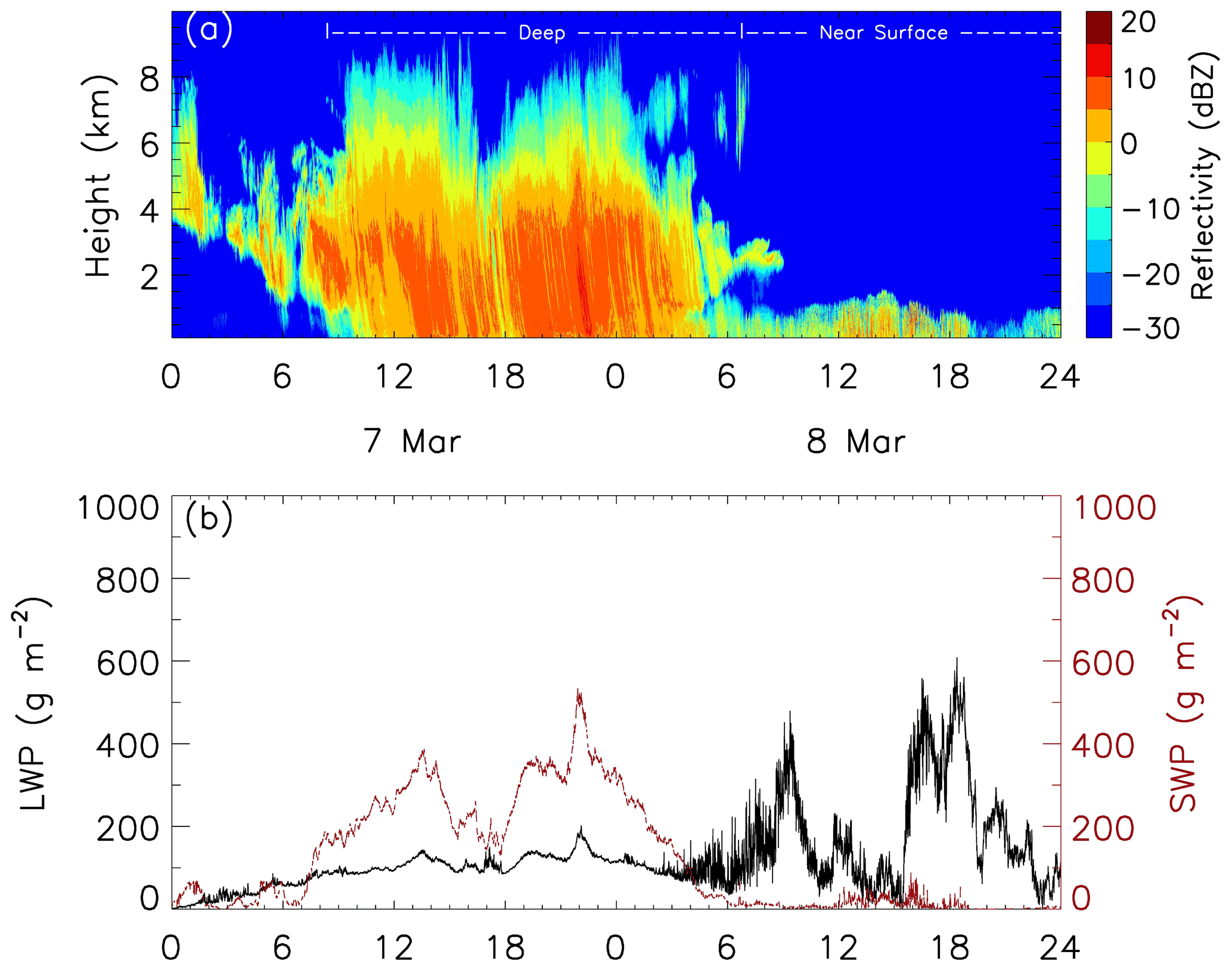
Figure 4 (a) Height–time cross section of radar reflectivity and (b) time series of the liquid water path (LWP, black) and snow water path (SWP, red) for observations on 7 and 8 March 2018.

3.1.2 Deep and “wet” followed by shallow snow clouds

On 28 February 2018, deep snow clouds associated with a low-pressure system were observed at the radar site, followed by shallow snow clouds that lasted till 03:00 UTC on 1 March. Radar reflectivity, the liquid water path, and snow water path are shown in Fig. 5. Surface PARSIVEL observations indicated melting snow with a surface air temperature near 0 ^∘C before 04:00 UTC on 28 February, which may have contributed to the liquid water path peak around 04:00 UTC. Heavy snowfall was observed from 04:00 to 14:00 UTC on 28 February; snowflakes observed at the surface level are large aggregates and show indications that riming occurred. The liquid water path was high for both the deep and shallow clouds with peaks higher than 400 g m⁻² even without including the portion of melting snow before 04:00 UTC on the 28th. Rimed snow particles were observed at the surface level which corresponded with the shallow snow cell based on 2DVD and MASC data.

Figure 5 (a) Height–time cross section of radar reflectivity and (b) time series of the liquid water path (LWP, black) and snow water path (SWP, red) for observations from 27 February through 1 March 2018.

3.2 Liquid versus ice in snow clouds

During the 6 month period, a total of 374 h of snow precipitation had been observed by the RPG-FMCW. The frequency distributions of 5 min averaged surface snowfall rates and liquid water paths are shown in Fig. 6 with both the surface snowfall rate and liquid water path in a logarithm scale. On average, deeper clouds generate heavier snowfall; near-surface and shallow snow clouds produce snowfall rarely heavier than 0.5 mm h⁻¹, while the snowfall rate in deep snow clouds reaches over 1 mm h⁻¹. Higher values of the cloud liquid water path are also more likely observed in deeper clouds. However, the likelihood of a substantial amount of liquid water in shallower clouds is also high. For example, for the liquid water path range of 100–250 g m⁻², the frequency values still reach about 10 % for near-surface and shallow snow clouds. At the upper limit, the liquid water path in all clouds only occasionally exceeds 500 g m⁻².

Figure 6 Frequency distribution of (a) the liquid water path and (b) the snowfall rate at the surface level derived from all observed snowfall data during the 2017–2018 winter. The frequency values are normalized so that the sum of their values at all bins is 100 %.

In Fig. 7, we show the scatterplot of the surface snowfall rate versus the liquid water path averaged over a 5 min period. As indicated in case studies earlier, the two variables hardly vary in a correlated fashion, neither positively nor negatively. For deep snow clouds, the heaviest snowfall corresponds to a liquid water path of about 200 g m⁻², while a further increase in the liquid water path does not seem to enhance surface snowfall. For shallow and near-surface snow clouds, the snowfall rate is confined between 0 and 0.6 mm h⁻¹, while the liquid water path stretches from 0 to 600 g m⁻² without coherent variation between the liquid water path and surface snowfall rate. Additionally, unlike heavy snowfall preferably occurring in deep snow clouds, large values of the liquid water path (say >300 g m⁻²) are almost equally probable to be found in near-surface, shallow, and deep snow clouds.

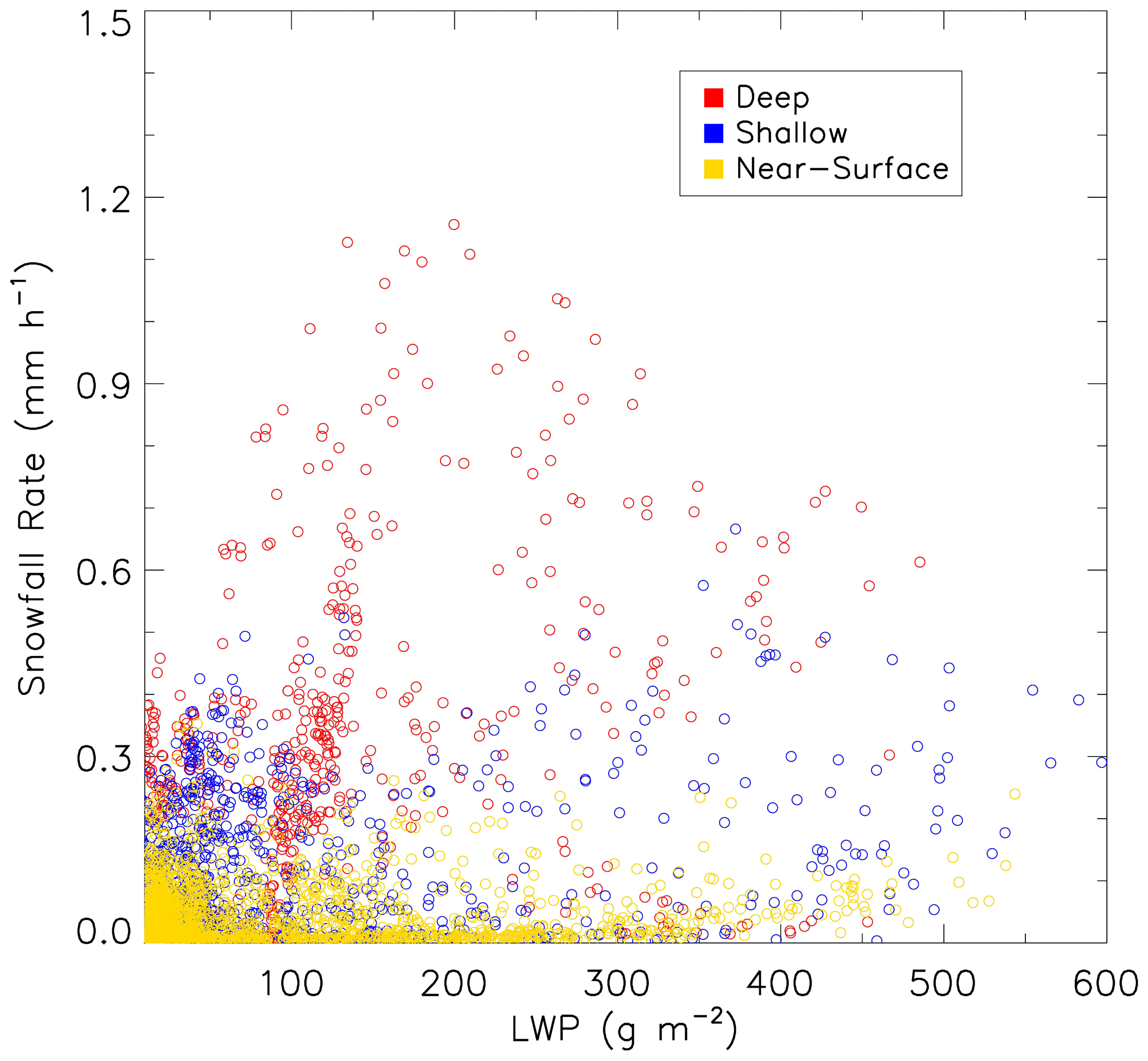
Figure 7 Scatterplot of the liquid water path and surface snowfall rate. Each point is an average of the 5 min data. All observed data during the 2017–2018 winter are included.

The mean state and its variability in cloud liquid water are also examined in the two-dimensional space of near-surface radar reflectivity and cloud top height, as shown in Fig. 8. In this figure, the mean values of (a) the number of occurrences, (b) the liquid water path, and (c) standard deviation of the liquid water path in each 2 dBZ by 500 m grid are shown based on the 5 min averaged data. The number of occurrences diagram indicates that heavier snowfall (stronger radar reflectivity) tends to have a higher cloud top for cases with near-surface radar reflectivity greater than 0 dBZ, although this tendency is not clear for cases with lower values of near-surface radar reflectivity. The diagrams for the mean and standard deviation of the liquid water path shown in Fig. 8b and c appear to indicate the following. For deep snow clouds (tops higher than 4 km) with surface radar reflectivity greater than 6 dBZ, the liquid water path has a large mean value but a small standard deviation. On the other hand, shallow snow clouds (tops between 1.5 and 4 km) with moderate surface radar reflectivity (0–5 dBZ) have a moderate mean value but a high variability in the liquid water path. There is an area with a high mean value and high variability in the liquid water path located at a surface radar reflectivity between −10 and 0 dBZ and at a cloud top height between 4 and 6 km, possibly corresponding to convective cells in early stages of development. For near-surface and shallow clouds, both the mean value and standard deviation of the liquid water path appear to increase as surface radar reflectivity increases.

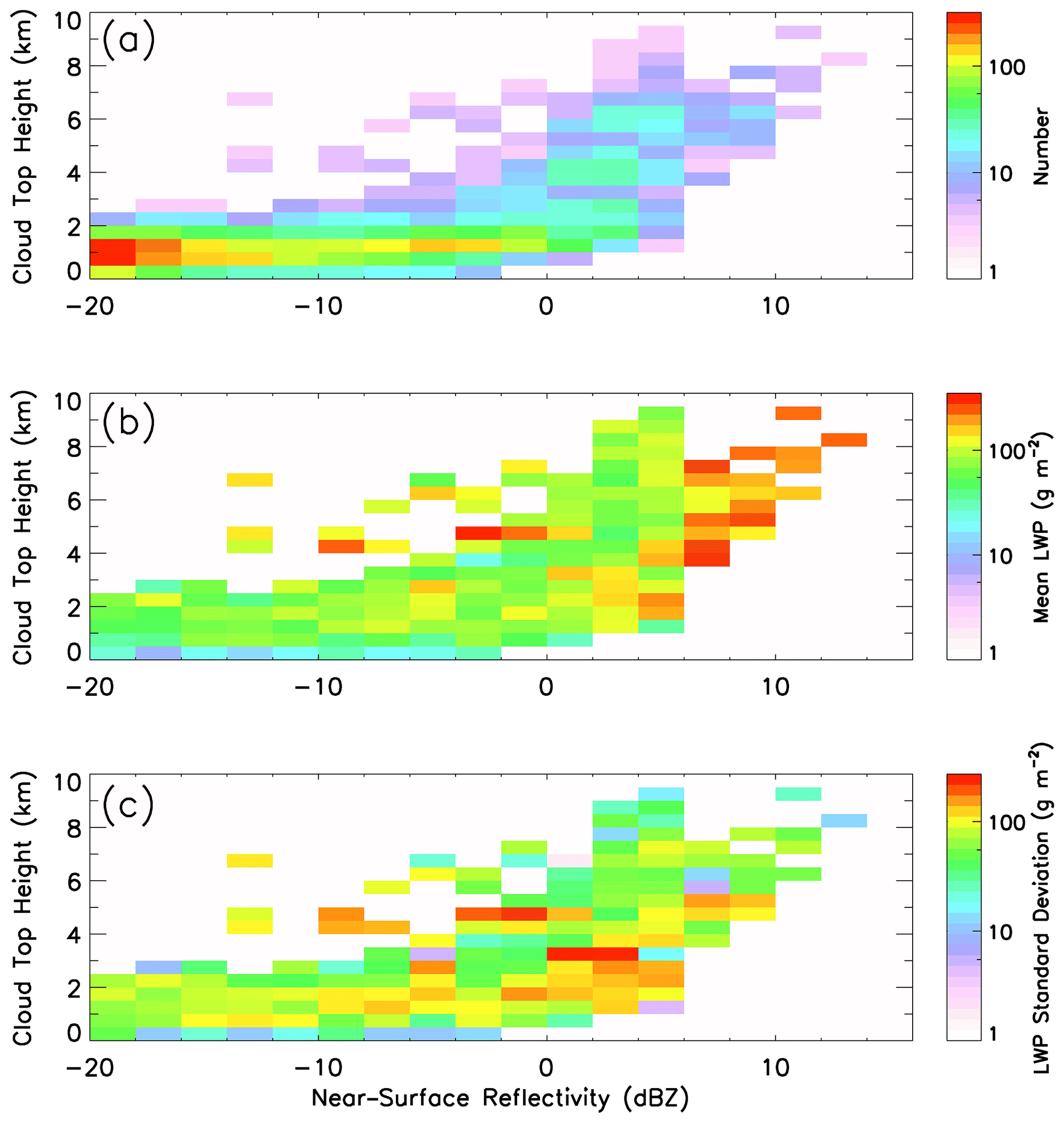
Figure 8 Two-dimensional distributions of (a) number of occurrences, (b) the liquid water path, and (c) standard deviation of the liquid water path as a function of near-surface radar reflectivity and cloud top height. All observed data during the 2017–2018 winter are used to calculate the distributions.

To express the “dryness” of the snow clouds, one may use the glaciation ratio (GR) defined as the following (Liu and Takeda, 1988):

$$\begin{array}{}\text{(5)}& \mathrm{GR}={\displaystyle \frac{\mathrm{SWP}}{\mathrm{LWP}+\mathrm{SWP}}}\times \mathrm{100}\mathit{\%}.\end{array}$$

The GR parameter indicates the fraction of total condensed water in the column that has been converted to solid phase. In Fig. 9, we show how the GR values are related to (a) cloud top height, (b) surface snowfall rate, and (c) cloud mean temperature (temperature at the geometrical middle of a reflectivity profile). Generally speaking, clouds with higher tops, associated with a higher snowfall rate or with colder mean temperature, tend to have higher degrees of glaciation, although the scatters are extremely large. For example, for a shallow snow cloud with a 0.2 mm h⁻¹ snowfall rate, its glaciation ratio can be any value from near 0 to about 100 %, probably depending on the development stage of individual cells. In Fig. 9a, there is a concentration of points with high cloud tops (>5 km) but with a glaciation ratio between 50 % and 75 % rather than 100 %. It is likely that the phenomena are caused by clouds that have multiple layers or a cloud layer with dynamically decoupled upper and lower portions. Corresponding to the clouds with their heaviest snowfall rate, deep snow clouds have a glaciation ratio of about 60 %, while shallow and near-surface snow clouds only have their glaciation ratio less than 20 %, which adds extra difficulties for detecting snow in these types of clouds by passive microwave observations. There is loosely a trend that clouds with a lower mean temperature have a higher degree of glaciation. For near-surface snow clouds, this trend is less clear with their glaciation degree hardly over 50 %. Using data observed over Greenland, Pettersen et al. (2018) found that snowfall events for frontal deep clouds are often ice clouds with little liquid water, while shallower clouds are typically mixed-phase clouds and contain plenty of supercooled liquid water. Their low glaciation rate for shallower clouds is similar to the results of this study.

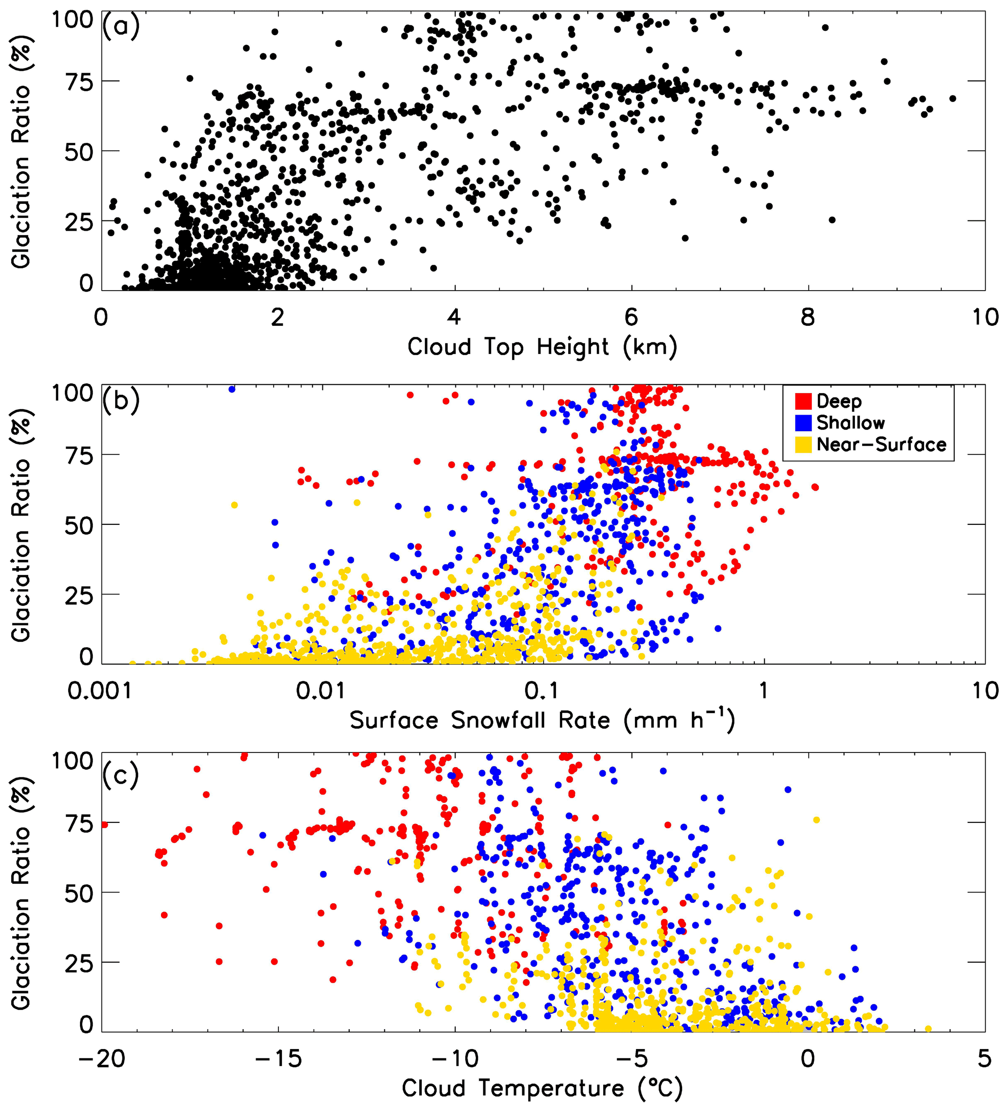
Figure 9 Scatterplot of glaciation ratio (see definition in the text) with (a) cloud top height, (b) surface snowfall rate, and (c) cloud temperature based on 5 min averages of all observational data of snow clouds in the 2017–2018 winter.

3.3 Vertical structures

The mean vertical structure of the snow clouds may be expressed with contoured frequency by altitude diagrams (CFADs; Yuter and Houze, 1995) of radar reflectivity, mean Doppler velocity, and Doppler spectral width, as shown in Fig. 10. For deep snow clouds, the radar reflectivity CFADs show a relatively narrow spread with a sharp radar reflectivity decrease with the increase in altitude above 4 km (“left-tilting” structure), implying that most of the precipitation growth occurs above 4 km. For shallow clouds, the “left-tilting” structure starts from near the surface, and the frequency has a broader distribution at each level. In contrast, the near-surface snow clouds do not show such “left-tilting” structure but rather have a broad distribution below their cloud top height, indicating that the precipitation maximum is not necessarily situated near the surface in these profiles. We interpret that the broad distribution of frequencies at each level is likely due to the convective nature of these clouds so that the precipitation profile is largely determined by the development stage of the clouds. For example, developing clouds have their precipitation maximum in the upper portion, while mature clouds have their precipitation maximum in the lower portion in the vertical profiles.

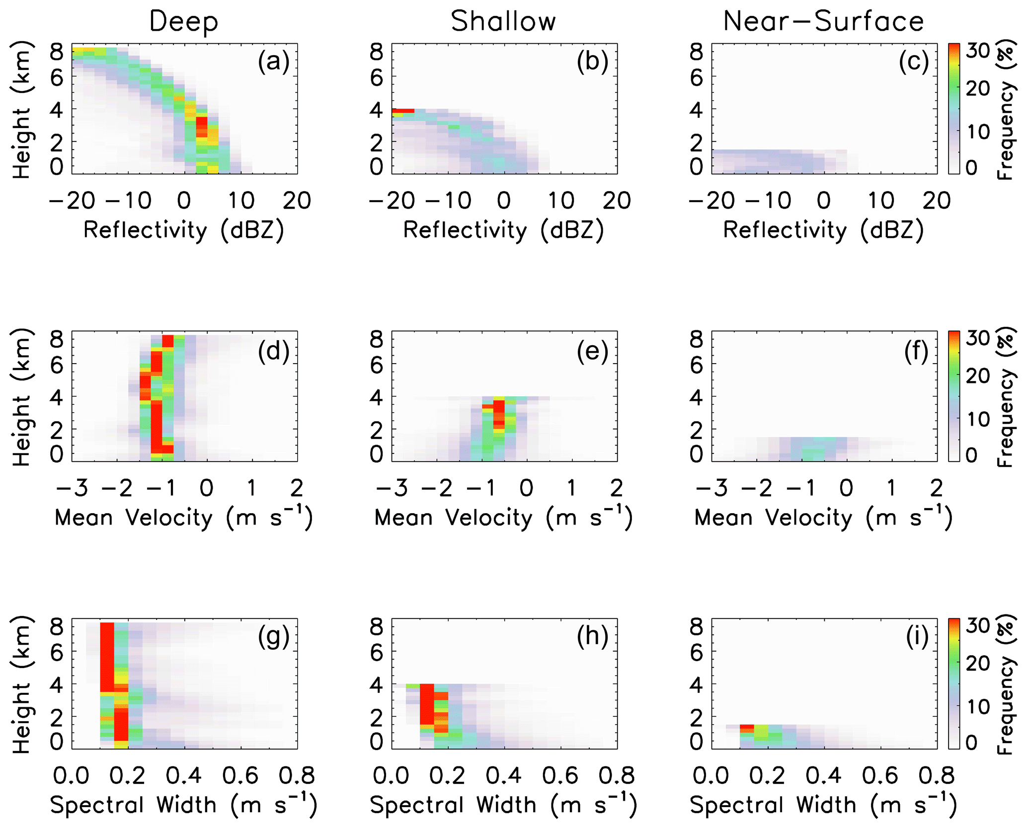
Figure 10 Contoured frequency by altitude diagrams (CFADs) for radar reflectivity (a, b, c), mean Doppler velocity (d, e, f), and Doppler spectral width (g, h, i) for deep (a, d, g), shallow (b, e, h), and near-surface (c, f, i) snow clouds. The frequency values are calculated in such a way that the sum of all frequency values at each altitude is 100 %. All observed data from the 2017–2018 winter are used.

For mean Doppler velocity, the most likely values are around −1 m s⁻¹ (the negative sign indicates downward movement), corresponding to the terminal velocity of unrimed to moderately rimed aggregates (Locatelli and Hobbs, 1974). There is a tendency that particles at upper levels fall somewhat slower than those at the lower levels. The Doppler spectral width indicates that particles at the upper levels have a narrower spectrum. Combining the vertical profiles of mean Doppler velocity and spectral width, it is concluded that ice particles at upper levels have a narrower size distribution and lower terminal velocity. It is also interesting to note that there seems to be a regime shift for deep snow clouds near 4 km altitude; the frequency patterns appear to be different below and above this level for all the CFADs of radar reflectivity, Doppler velocity, and spectrum width. Additionally, the slope of reflectivity suddenly changes at around 8 km, and the absolute value of Doppler velocity reduced dramatically below 8 km. A similar feature also appeared in the long-term observations with cloud radar (see Figs. 16 and 17 of Ye et al., 2020). The shift in growth regime appeared at 8 km height (3–3.5 km above the bright band peak and corresponding to $\sim -\mathrm{17}$ ^∘C). This regime shift induced the updraft (reached 1 m s⁻¹) below this layer. However, Ye et al. (2020) could not explain the linkage between this regime shift and updraft below. While it is beyond the scope of this study, this phenomenon will be an interesting topic for future research on cloud microphysics in this region.

4 Implications for passive microwave remote sensing

To understand how the microphysical properties in snow clouds impact on passive microwave remote sensing, a radiative transfer model simulation at GPM/GMI channels has been conducted using the measured liquid and snow water quantities as a guidance for the model input. The radiative transfer model developed by Liu (1998) has been used in this simulation, which uses a four-stream discrete ordinates method to solve the radiative transfer equation. For snow particles, the single-scattering properties calculated by discrete dipole approximation for sector-type snowflakes (Liu, 2008b) are used. Based on the study by Geer and Baordo (2014), the single-scattering properties for the sector type snowflakes work reasonably well in radiative transfer simulations for middle latitude snowstorms. Since the emphasis of this study is to assess the impact of cloud microphysics on satellite remote sensing, the variability of surface emissivity is not considered. In all the following simulations, we assign an emissivity of 0.9 for land surface for all GMI channels and a 5 m s⁻¹ wind speed over ocean to compute surface emissivity.

4.1 Masking effect to scattering signatures by cloud liquid water

Based on the analysis shown in Sect. 3.2, the liquid water path frequently varies from 0 to 500 g m⁻² for any of the three types of snow clouds, while the snowfall rate at the surface level commonly reaches 0.3, 0.5, and 1.0 mm h⁻¹, respectively, for near-surface, shallow, and deep clouds. We examine how the cloud liquid would mask the ice scattering at two GMI frequencies, 89 and 166 GHz at viewing angles of 53^∘ for 89 GHz and 49^∘ for 166 GHz, using radiative transfer calculations. Using clear-sky brightness temperature T_B0 as the base, Fig. 11 shows how brightness temperature varies as the liquid water path and surface snowfall rate increase. Note that in these radiative transfer calculations, mean snowfall rate profiles derived from observations are used. The mean profiles are derived as follows. We first group all the observed snowfall rate profiles according to their cloud type, and then for each cloud type, we average those profiles that fall into a given snowfall rate bin. A 1 km deep liquid cloud layer is placed at 0.5–1.5 km, 2.5–3.5 km, and 4.5–5.5 km, respectively, for near-surface, shallow, and deep clouds. The liquid water path is increased from 0 to 500 g m⁻².

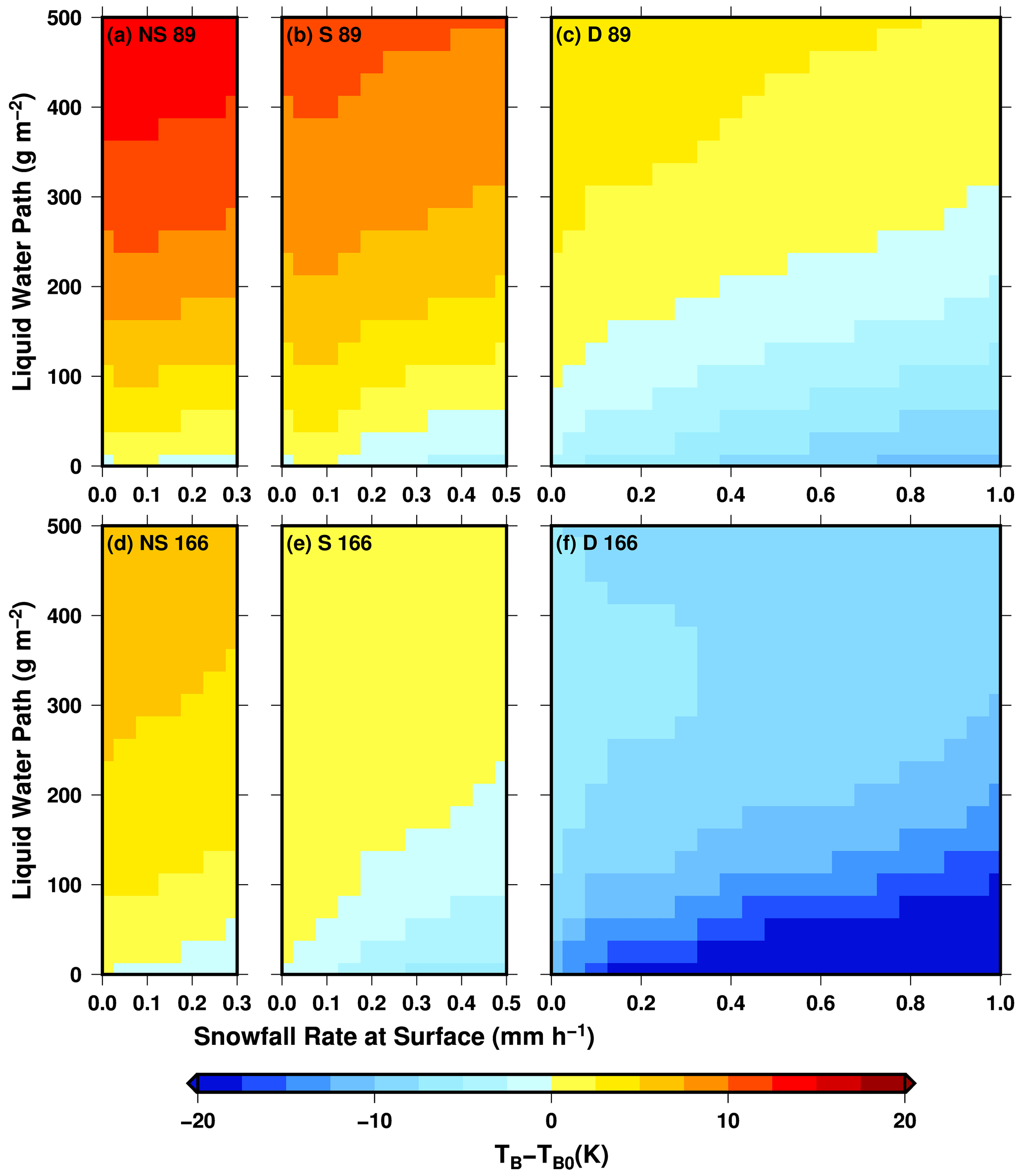
Figure 11 Simulated brightness temperature change (relative to clear-sky values) at GMI 89 GHz (a, b, c) and 166 GHz (d, e, f) for near-surface (a, d), shallow (b, e), and deep (c, f) snow clouds. The change is relative to clear-sky values.

For near-surface snow clouds, the decrease in brightness temperature due to ice scattering is very limited for either 89 or 166 GHz, with only about 1.5 K for 89 GHz and 2.5 K for 166 GHz occurring when the liquid water path is very low. Therefore, most likely this type of cloud displays a warming signature in the passive microwave observations due to the existence of liquid water clouds. For shallow snow clouds, the modeling results show there is still mostly warming at 89 GHz and an equal mix of warming and cooling at 166 GHz. The masking effect still remains quite significant at 89 GHz even for deep snow clouds; it can cause an increase in brightness temperature by more than 5 K from clear-sky values. The dominant scattering signature shows at 166 GHz for deep clouds. At a surface snowfall rate of 1 mm h⁻¹, brightness temperature can decrease from the clear-sky values by more than 30 K (color bar only shows up to −15 K) when the liquid water path is lower than 100 g m⁻².

Based on the above modeling results, it is clear that if only relying on scattering signature, i.e., brightness temperature depression, an algorithm will totally fail in retrieving the snowfall rate for near-surface clouds and partially fail for shallow clouds. Even for deep snow clouds, cloud liquid water will impact snowfall retrieval with the result of an overestimation for low and an underestimation for high values of the liquid water path. Therefore, a more plausible approach to the retrieval problem is to use a statistical method in which the algorithm utilizes any regularities naturally existing between cloud liquid and snow profiles to search for the most likely snowfall rate. One such approach is the Bayesian retrieval algorithm (Kummerow et al., 1996; Olson et al., 1996; Seo and Liu, 2005). This approach requires that the a priori database used in the retrieval has the same characteristics in both microphysical properties and occurrence frequency as those in natural clouds.

4.2 A Bayesian retrieval exercise

In this section, an idealized experiment is designed to examine how a Bayesian retrieval algorithm would perform for the three types of snow clouds if we only take into account the error caused by the variability of the liquid water path and snowfall rate profiles. In other words, we examine how well a Bayesian retrieval algorithm would perform, when assuming no variations in surface emissivity, snowflakes being a fixed type, and particle size distribution following an exponential form. Therefore, this exercise mainly assesses the problems caused by the uncertainties associated with cloud liquid and snow amounts.

First, a total of 30 870 5 min averaged snow profiles are constructed from the 6-month-long surface radar observations (including zero snowfall profiles). Each of the snow profiles is accompanied by a liquid water path which is assigned to be a 1 km deep layer at 0.5–1.5 km, 2.5–3.5 km, and 4.5–5.5 km, respectively, for near-surface, shallow, and deep clouds. Atmospheric temperature, pressure, and relative humidity profiles are also assigned to these profiles by interpolating MERRA-2 data spatially and temporally to the individual snow profiles. A radiative transfer model calculation is then performed to generate brightness temperatures at 11 GMI channels (all except the 10.7 GHz GMI channels) using the above profiles as input. The 10.7 GHz channel is not considered here because its brightness temperature is not sensitive to either liquid or ice hydrometeors, and its GMI channel has too large a footprint size compared to other channels. It is also assumed that surface skin temperature is the same as surface air temperature and surface emissivity is a constant (0.9 for land) for all channels. A sector type snowflake (Liu, 2008b) and an exponential particle size distribution (Sekhon and Srivastava, 1971) are used for all the cases. We then randomly divided the 30 870 profiles and their computed brightness temperatures into two equal-number groups: one is used as the a priori database for the Bayesian retrieval algorithm, and the other as “observations” to test how well the surface snowfall rate can be retrieved from the “measured” brightness temperatures. To mimic a possible random error in the measured brightness temperatures, a random noise with a maximum magnitude of 1 K is added to the measured brightness temperatures before retrieval is performed. A detailed description of the Bayesian retrieval method can be found in Seo and Liu (2005).

In Fig. 12, the scatterplots of measured versus retrieved surface snowfall rates separated by snow cloud types are shown. The correction, as indicated by R² (square of linear correlation coefficient), bias, and root mean square (RMS) difference are shown in each diagram. The biases between the measured and retrieved snowfall rate are small for all snow cloud types with values of 0.019, 0.033, and 0.03 mm h⁻¹ for near-surface, shallow, and deep snow clouds, respectively. The values of RMS differences are also small; they are 0.05, 0.11, and 0.16 mm h⁻¹, respectively, for near-surface, shallow, and deep snow clouds. The color of the points in the figures indicates the value of the liquid water path associated with individual profiles. Clearly, as the cloud layer deepens, the skill of the retrieval improves. The values of R² increase from 0.32 for near-surface clouds, to 0.41 for shallow clouds, and to 0.62 for deep clouds. That is to say that the retrievals can resolve 32 %, 41 %, and 62 % of the variances in snowfall rate observations for near-surface, shallow, and deep clouds, respectively.

Figure 12 Scatterplot of measured versus retrieved snowfall rates for (a) near-surface, (b) shallow, and (c) deep snow clouds over land. The color of the points indicates the liquid water path associated with the case. The correlation is indicated by R² in each diagram. Biases and root mean square (RMS) differences are also indicated in the diagrams.

A question one may naturally want to ask is whether the retrieval skill will be improved if the same clouds were moved to areas over ocean where liquid water information is distinguishable at some microwave channels (e.g., 89 GHz). To answer this question, we perform the same retrieval exercise as mentioned above but assuming the clouds are over an ocean surface with a constant surface wind speed of 5 m s⁻¹. Similarly, half of the 30 870 samples are used as an a priori database and half as observations. The retrieval results are shown in Fig. 13. Similar to land cases, the biases and RMS differences have small values for all cloud types. For deep snow clouds, the R² statistic indicates only a small improvement in retrieval skills between cases over land and over ocean, although a visual inspection of the scatterplot shows that a better correspondence between measured and retrieved values at snowfall rates lower than 0.2 mm h⁻¹. The improvement in retrieval skills for over ocean shallow clouds is moderate with R² of 0.54 versus 0.41 over land. The most significant improvement in retrieval skills occurs for over ocean near-surface snow clouds, in which R² increases from 0.32 over land to 0.52 over ocean. Note that land surface emissivity and ocean surface wind are fixed in the retrieval exercises. Therefore, the improvement is not due to a better knowledge of surface conditions but rather due to the richer information content on cloud microphysics contained in measured brightness temperatures over ocean. One such piece of information must have come from the brightness temperature difference between two polarizations over ocean, which remains mostly zero over land surfaces. The results shown in Fig. 13 indicate that the extra polarization information helps the most for retrieving snowfall in shallower clouds.

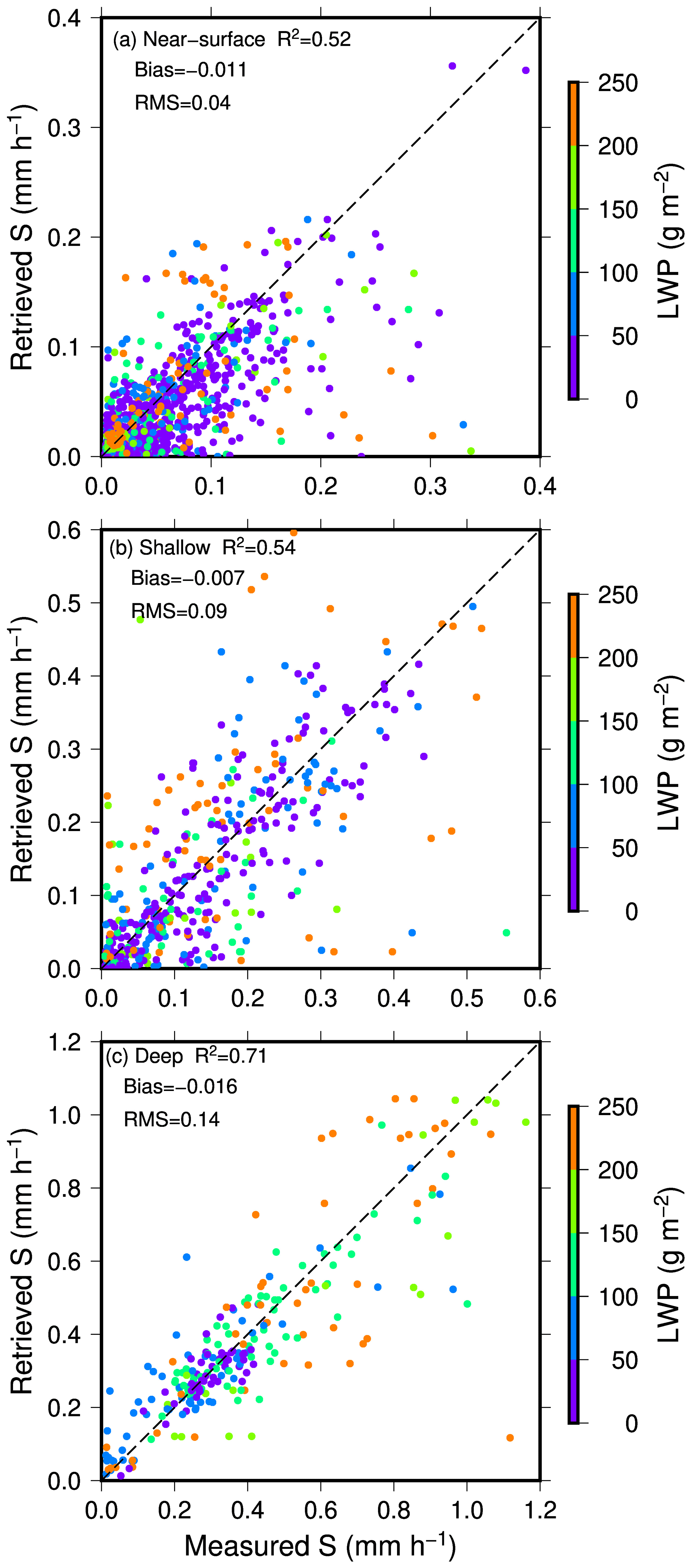
Figure 13 Scatterplot of measured versus retrieved snowfall rates for (a) near-surface, (b) shallow, and (c) deep snow clouds over ocean. The color of the points indicates the liquid water path associated with the case. The correlation is indicated by R² in each diagram. Biases and root mean square (RMS) differences are also indicated in the diagrams.

In Figs. 12 and 13, it is also noted that an underestimation occurs when the snowfall rate is greater than 0.7 mm h⁻¹ for deep snow clouds regardless if over land or ocean. This underestimation may be due to the deficiency of the Bayesian scheme, in which the retrieval is a weighted average of snowfall rates of datum points in the a priori database that are radiometrically consistent with observations. When an observation is close to the upper boundary (i.e., high snowfall rates) in the database, the averaging takes a greater number of datum points with snowfall rates lower than the actual value than those with higher snowfall rates (no more datum points beyond upper boundary), thus resulting in an underestimation.

To understand the information conveyed in the polarization difference of brightness temperatures, we performed a similar simulation to that described in Sect. 4.1 but replaced land surface with ocean surface with a wind speed of 5 m s⁻¹. The changes in depolarization as the liquid water path and snowfall rate increase are shown in Fig. 14 for each of the three cloud types at 89 and 166 GHz. Depolarization is defined as $\mathrm{\Delta }{T}_{\mathrm{B}}=T_{\mathrm{BV}}-T_{\mathrm{BH}}$, where T_BV and T_BH are brightness temperatures at vertical and horizontal polarizations, respectively. The change is relative to clear-sky values, ΔT_B0. The change in depolarization at 89 GHz corresponds well with the change in the liquid water path without much dependence on snowfall rate, particularly for near-surface and shallow snow clouds. Therefore, it is plausible that the increased retrieval skill over ocean for near-surface and shallow clouds is due to the added information on liquid water contained in the polarization differences. Comparing Figs. 12 and 13, it seems that the added information is particularly helpful in improving retrievals at low snowfall rates.

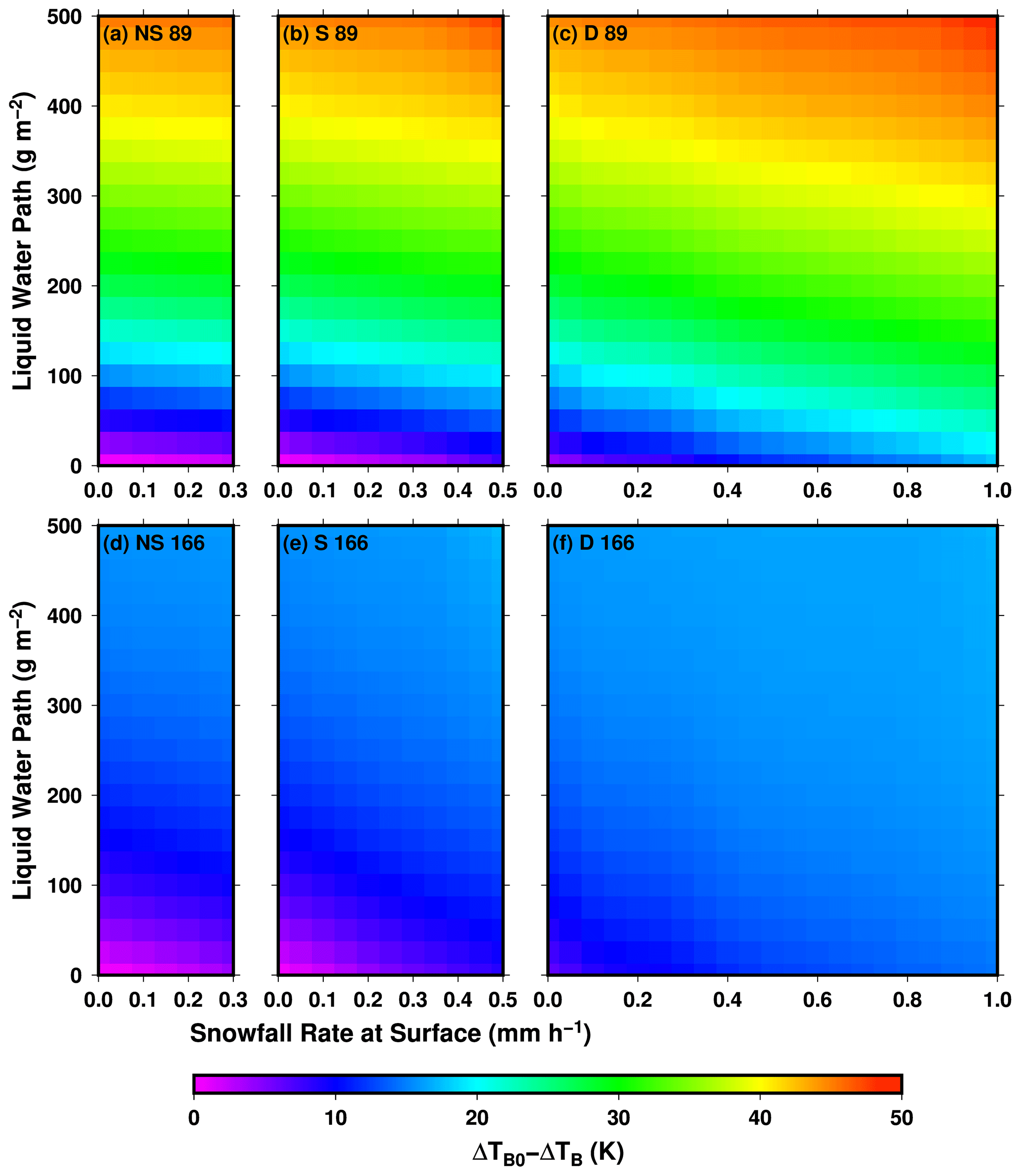
Figure 14 Simulated change of depolarization for GMI 89 GHz (a, b, c) and 166 GHz (d, e, f)  for near-surface (a, d), shallow (b, e), and deep (c, f) snow clouds over ocean. Depolarization is the brightness temperature difference between vertical and horizontal polarizations. The change is relative to clear-sky values.

5 Conclusions

During the 2017–2018 winter season, a ground-based radar and radiometer observation was carried out over the Korean Peninsula as part of the ICE-POP 2018 campaign. Using the coincident radar and radiometer data, we were able to retrieve the cloud liquid water path, snow water content, and snowfall rate. These microphysical properties and their relation to cloud top height are analyzed in an effort to better understand their implications for the satellite remote sensing of snowfall. In the analysis, we divide the approximately 374 h of observed snow clouds into near-surface, shallow, and deep types, for which the cloud top height is below 1.5 km, between 1.5 and 4 km, and above 4 km, respectively. The near-surface snow clouds are most likely to be missed by currently available space-borne radars because of the blind zone caused by the contamination of surface clutter, and their shallowness and liquid water abundance may also present challenges to satellite radiometer observations. In this region during the observation period, the shallow snow clouds commonly occur in an unstable air mass after the passing of a cold front. It can be detected by space-borne radars with sufficiently low minimum detectable radar reflectivity, but the mixture of cloud liquid emission and ice scattering complicates the retrievals by passive microwave observations. The deep snow clouds are mostly located near frontal zones and low-pressure centers; their strong ice scattering signature makes it the most favorable type among the three for snowfall retrievals by both satellite radars and radiometers. Surveying all the observed data, it is found that near-surface snow clouds are the most frequently observed cloud type with a frequency of occurrence over 60 %, while deep snow clouds contribute the most in snowfall volume with about 50 % of the total snowfall amount.

The probability distributions of surface snowfall rates are clearly different among the three types of snow clouds, with the vast majority of them hardly reaching 0.3 mm h⁻¹ for near-surface, 0.5 mm h⁻¹ for shallow, and 1 mm h⁻¹ for deep snow clouds. However, the liquid water paths in the three types of snow clouds all have the substantial likelihood to be between 0 to 500 g m⁻², although deeper clouds are somewhat more likely with more liquid water as well. There is no clear correlation, either positive or negative, between the surface snowfall rate and liquid water path. However, given the same surface snowfall rate, clouds with lower cloud top heights tend to have higher liquid water paths. The glaciation ratio defined by the ice fraction in the total condensed water in an atmospheric column is estimated and found to be related to cloud top height, surface snowfall rate, and cloud mean temperature, although the relations are very scattered. A higher value of glaciation ratio generally corresponds to a higher cloud top, a higher surface snowfall rate, and a lower cloud mean temperature.

Moreover, we examined the ability of a Bayesian-type algorithm to retrieve the surface snowfall rate for snow events similar to those observed in this study when using GPM/GMI observations. First, using the approximately 30 000 observed snow cloud and precipitation-free profiles, brightness temperatures at GPM/GMI channels are computed. Then, these snowfall rate and associated brightness temperature pairs are randomly divided into two groups. One group is used as observations and the other is used as the a priori database of the Bayesian algorithm. Under idealized scenario, i.e., without considering the uncertainties caused by surface emissivity, ice particle size distribution, and particle shape, the examination results indicate that the correlation as expressed by R² between the retrieved versus measured snowfall rates is about 0.32, 0.41, and 0.62, respectively, for near-surface, shallow, and deep snow clouds over land surfaces. Since this is an extremely idealized retrieval exercise only dealing with the complicated mixture of cloud liquid and snow profiles, these numbers basically indicate the upper limits of how a retrieval algorithm can perform for these snow clouds. A hypothetical retrieval for the same clouds but over ocean is also studied, and a major improvement in skill for near-surface clouds is found with R² increasing from 0.32 to 0.52, while an improvement in skill is small for deeper clouds. The improvement is interpreted as being the result of some liquid water information being resolved by the polarization difference contained in the brightness temperatures over ocean. This information helps the most for the otherwise information-poor observations for the near-surface clouds.

By analyzing the radar and radiometer data from yearly winter observations and the results of a Bayesian retrieval dry run, this study gives a general picture of the characteristics of the different types of snow clouds and points out the fundamental challenges in retrieving their snowfall rate from passive microwave observations. It is hopeful that these results can help developers improve physical assumptions in future algorithms, as well as help data users better interpret satellite-retrieved snowfall products. Lastly, it is worth mentioning that there are still many valuable datasets, such as particle shape and size distribution information from PARSIVEL, 2DVD, and MASC, which we did not analyze quantitatively in this study. A thorough analysis of those datasets in conjunction with the remote sensing data will undoubtedly improve future snowfall retrieval algorithm development.