the Creative Commons Attribution 4.0 License.
the Creative Commons Attribution 4.0 License.
 | 11 Nov 2020
Volatile organic compound fluxes in a subarctic peatland and lake
Thomas Holst
Mikkel Sillesen Matzen
Andreas Westergaard-Nielsen
Tihomir Simin
Joachim Jansen
Patrick Crill
Thomas Friborg
Janne Rinne
Riikka Rinnan
Ecosystems exchange climate-relevant trace gases with the atmosphere, including volatile organic compounds (VOCs) that are a small but highly reactive part of the carbon cycle. VOCs have important ecological functions and implications for atmospheric chemistry and climate. We measured the ecosystem-level surface–atmosphere VOC fluxes using the eddy covariance technique at a shallow subarctic lake and an adjacent graminoid-dominated fen in northern Sweden during two contrasting periods: the peak growing season (mid-July) and the senescent period post-growing season (September–October).
In July, the fen was a net source of methanol, acetaldehyde, acetone, dimethyl sulfide, isoprene, and monoterpenes. All of these VOCs showed a diel cycle of emission with maxima around noon and isoprene dominated the fluxes (93±22 µmol m−2 d−1, mean ± SE). Isoprene emission was strongly stimulated by temperature and presented a steeper response to temperature (Q10=14.5) than that typically assumed in biogenic emission models, supporting the high temperature sensitivity of arctic vegetation. In September, net emissions of methanol and isoprene were drastically reduced, while acetaldehyde and acetone were deposited to the fen, with rates of up to µmol m−2 d−1 for acetaldehyde.
Remarkably, the lake was a sink for acetaldehyde and acetone during both periods, with average fluxes up to µmol m−2 d−1 of acetone in July and up to µmol m−2 d−1 of acetaldehyde in September. The deposition of both carbonyl compounds correlated with their atmospheric mixing ratios, with deposition velocities of and cm s−1 for acetone and acetaldehyde, respectively.
Even though these VOC fluxes represented less than 0.5 % and less than 5 % of the CO2 and CH4 net carbon ecosystem exchange, respectively, VOCs alter the oxidation capacity of the atmosphere. Thus, understanding the response of their emissions to climate change is important for accurate prediction of the future climatic conditions in this rapidly warming area of the planet.
- Article
(2344 KB) - Full-text XML
-
Supplement
(959 KB) - BibTeX
- EndNote


Arctic climate is warming twice as fast as the global average (Post et al., 2019). This is due to a number of climate system feedbacks, including (i) albedo change due to retreating snow cover and sea ice and (ii) the forest cover expansion to the open tundra (Overland et al., 2014; Post et al., 2009). Northern ecosystems are known to exchange climate-relevant trace gases with the atmosphere, not only long-lived greenhouse gases such as carbon dioxide (CO2) or methane (CH4) but also hundreds of different volatile organic compounds (VOCs) that are a highly reactive part of the carbon cycle (Rinnan et al., 2014). Trace gases originate from sources as diverse as soils, peats, vegetation, and lakes, and currently several of them show a trend towards greater emission rates with climate warming (Kramshøj et al., 2019; Lindwall et al., 2016a; Wik et al., 2016). At the same time, the warming-induced expansion of woody shrubs into tundra ecosystems (Myers-Smith and Hik, 2018) could enhance the photosynthetic uptake of CO2 and offset concurrent increases in heterotrophic respiration (Mekonnen et al., 2018). Indeed, CO2 and CH4 have been extensively surveyed in high latitudes due to a potential increase in their atmospheric concentrations and connected climatic effects as permafrost thaws (Natali et al., 2019; Schuur et al., 2015). In contrast, far less research has been devoted to VOC emissions in these areas.
VOCs play essential ecological roles: they can mediate the communication between living organisms and protect plants from biotic and abiotic stresses (Baldwin et al., 2006; Filella et al., 2013; Kessler and Baldwin, 2001; Peñuelas et al., 2005b; Pichersky and Gershenzon, 2002; Seco et al., 2011b; Velikova et al., 2005). In addition, biogenic VOCs engage in chemical reactions that substantially modify the oxidation capacity of the atmosphere. For example, VOCs enhance the lifetime of methane by competing for its atmospheric oxidants, promote the formation of tropospheric ozone, and ultimately contribute to aerosol formation in the atmosphere, which has climatic consequences (Atkinson, 2000; Liu et al., 2016; Seco et al., 2011a; Tunved et al., 2006). Meanwhile, climate change is affecting the fundamental functions of VOCs and altering their emission rates in northern ecosystems, directly via warming and indirectly by inducing changes in vegetation composition (Faubert et al., 2010a; Li et al., 2019; Lindwall et al., 2016a; Valolahti et al., 2015). Moreover, the atmospheric impact of VOCs emitted from natural sources may be comparatively more important in northern latitudes than in more populated territories due to the relatively low presence of anthropogenic VOC emissions (Paasonen et al., 2013).
VOC studies over the last few years have reported strong increases in arctic and subarctic vegetation emissions in response to moderate warming (Faubert et al., 2010a; Kramshøj et al., 2016; Lindwall et al., 2016a), highlighting the capacity of Arctic plants to respond to increasing temperature. However, these studies have been conducted using enclosure techniques with a range of unwanted side effects, such as temperature and humidity rise inside the enclosure and interactions with chamber materials (Ortega and Helmig, 2008). Micrometeorological techniques such as eddy covariance (EC) can overcome many of those undesirable side effects and, in addition, provide a more representative ecosystem-level VOC exchange quantification by minimizing potential sampling error when upscaling from a small number of enclosures to ecosystem fluxes. However, instrumental challenges have limited the number of ecosystem-level VOC studies using EC, and only two such datasets over short time periods are available for high-latitude ecosystems (Holst et al., 2010; Potosnak et al., 2013). Moreover, there are few or no air–water direct VOC flux measurements from northern lakes. Arctic latitudes possess one of the highest concentration and area of inland water bodies of our planet (Verpoorter et al., 2014). Despite being acknowledged as important regional and global sources of carbon dioxide and methane (Tranvik et al., 2009; Wik et al., 2016), the role of northern lakes in the VOC budget is largely unexplored. It is therefore vital to assess the lake and vegetation VOC fluxes in these high-latitude areas exposed to large environmental changes to be able to estimate their impacts on the regional carbon cycle, atmospheric chemistry, and climate.
We report here ecosystem-level VOC fluxes measured by EC from a subarctic shallow post-glacial lake, a common lake form in the Arctic (Wik et al., 2016), and its adjacent fen dominated by tall graminoids. We aimed to identify which compounds were released at significant rates from the lake and which from the fen during two contrasting periods: the peak of the growing season (mid-July) and the senescent period post-growing season (September–October). Further, we assessed the deposition of compounds to the two ecosystems. In addition, we included here the EC fluxes of carbon dioxide and methane from both fen and lake, which have been discussed elsewhere (Jammet et al., 2015, 2017; Jansen et al., 2019a), to provide a more thorough overview of the trace gas fluxes during our study.
2.1 Site description and field campaign outline
Stordalen mire is a subarctic palsa mire complex underlain by discontinuous permafrost (Johansson et al., 2006). It is located ca. 10 km east of Abisko in northern Sweden (68∘20′ N, 19∘03′ E). Local meteorology has been monitored at the Abisko Scientific Research Station (ANS) with records since 1913 (Callaghan et al., 2010). The average air temperature at ANS during the period 1981–2010 was 0.1 ∘C and average annual rainfall 332 mm; the mean annual air temperature and precipitation at Stordalen in 2018 were −0.04 ∘C and 340 mm, respectively. The Stordalen mire was not affected by the drought that occurred in large parts of central and northern Europe during 2018 (Buras et al., 2020; Rinne et al., 2020).
Our measurements took place during the 2018 growing season from a 2.92 m tall eddy covariance mast located on the shore of a shallow post-glacial lake, Villasjön. The geomorphological setting within the Torneträsk catchment determines a bimodal distribution to the surface wind flow of roughly ESE and WNW (Fig. 1). The lake edge mast is influenced by Villasjön to the east and by fen to the west. The fen is a permafrost-free, minerotrophic wetland with vegetation dominated by tall graminoids, mainly Carex rostrata and Eriophorum angustifolium (Palace et al., 2018). The lake is 0.17 km2 in area, the largest of the 27 lakes that constitute the 15 km2 Stordalen catchment (Lundin et al., 2013). It has a maximum depth of 1.5 m and it usually freezes close to the bottom in winter (Jansen et al., 2019a). The bidirectional flow pattern throughout the year allows a clear distinction of the surface source or sink influences of the surface boundary layer. Thus, depending on the prevailing wind direction, the measured VOC flux data were assigned to either the lake or the fen (e.g. Jammet et al., 2015). Flux data originating outside of these wind directions, usually at very low wind speeds, contributed only a minor part of the total fluxes and were excluded from analysis. The average EC flux footprint used in our study (Fig. 1) was calculated with a two-dimensional model (Kljun et al., 2015); see the Supplement for further details.
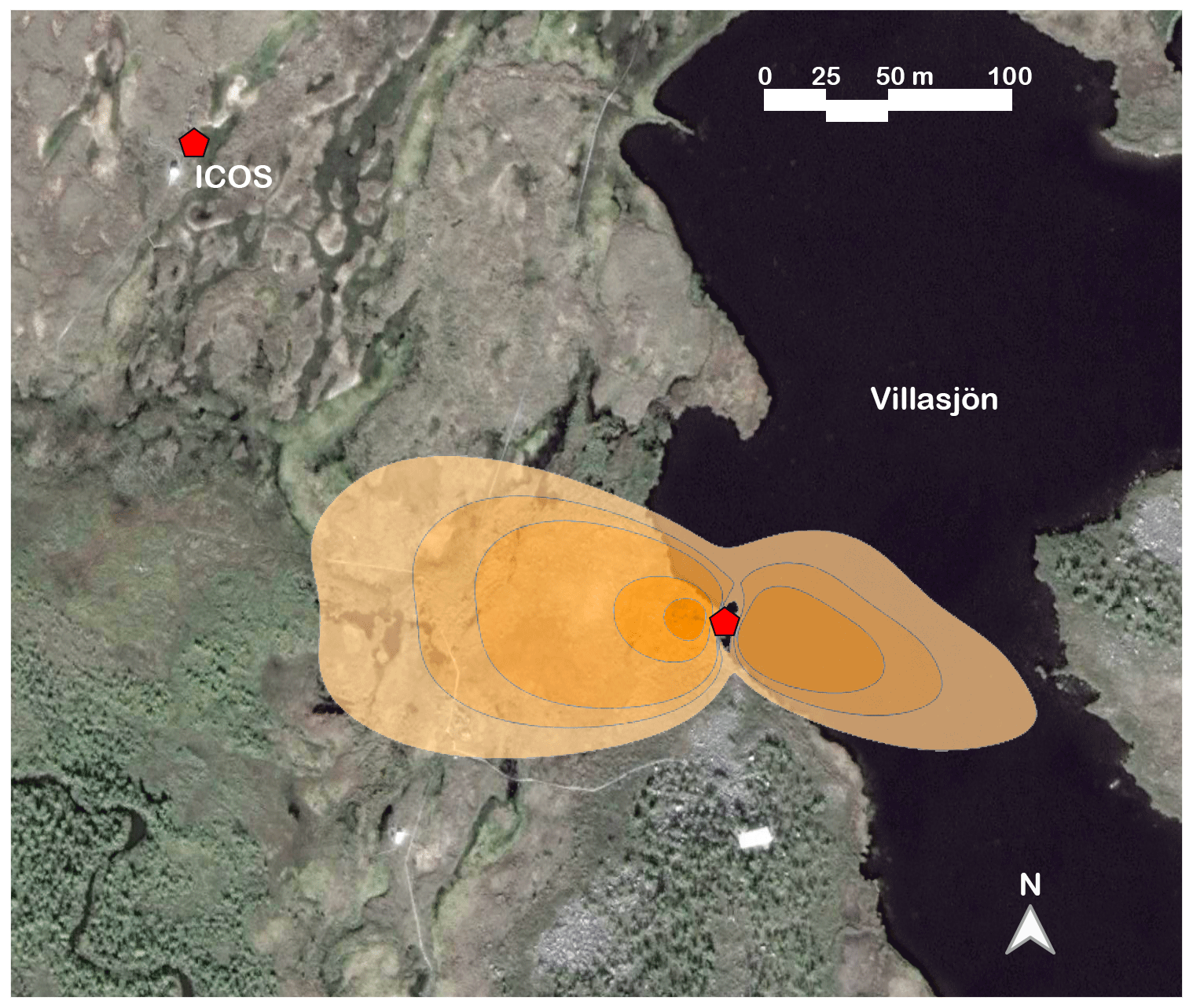
Figure 1Map of the Stordalen mire study area, showing our EC tower by the shore of Villasjön and the nearby ICOS station location that provided the vegetation surface temperature data. The shaded area represents the combined fen and lake footprint for the July EC measurements, at flux contribution intervals of 85 %, 80 %, 75 %, 50 %, and 25 %. The base map image is from © Google Earth (image provided by DigitalGlobe).
Several major instrumental issues precluded us from obtaining a season-long dataset of VOC fluxes. With the available data, when the instruments were operational, we present measurements from two distinct periods: the peak of vegetation activity (15–22 July) and the senescent period post-growing season (20 September–13 October). We determined the relative seasonal status of the vegetation at this site based on greenness data captured by an automatic camera installed on the EC mast (see Sect. 2.3 and Fig. S1 in the Supplement). For the sake of simplicity, in this article we will refer to the season peak period as July and to the post-growing season as September.
Considering the wind direction partitioning and the two periods for which we have data, the maximum number of half-hour EC fluxes in July were 64 and 246 for the lake and fen, respectively. In September, we had a maximum of 429 EC fluxes for the lake and 619 for the fen. However, since some VOC fluxes were discarded according to strict quality assurance procedures recommended for EC measurements (see Sect. 2.2), the actual number of valid half-hour VOC fluxes was smaller for individual chemical species (e.g. for isoprene in July, valid data points were 22 for the lake and 161 for the fen). VOC fluxes from the lake for July were only available for some hours of the day (between 03:00 and 14:00 UTC+1).
2.2 VOC measurements
Mixing ratios of VOCs were measured with a proton-transfer-reaction time-of-flight mass spectrometer (PTR-TOF-MS). This particular model (PTR-TOF 1000ultra, Ionicon Analytik, Innsbruck, Austria) was equipped with an ion funnel at the end of the drift tube that provided a higher sensitivity and had a compound (diiodobenzene) added continuously to the air sample that provided a constant signal at high mass-to-charge ratio (m∕z) for accurate TOF mass scale calibration. The drift tube was operated at 60 ∘C, 550 V, and 2.3 mbar. Multipoint sensitivity calibration was performed at least once a month (including at the end of the July period and before, midway, and at the end of the September period) by diluting a blend of several VOCs (e.g. methanol, acetaldehyde, acetone, isoprene, alpha-pinene, and benzene, among others, in nitrogen at a VOC mixing ratio of mol mol−1 each, manufactured by Ionicon Analytik) into clean nitrogen. The dilution (range 1–40 × 10−9 mol mol−1) was achieved with a Liquid Calibration Unit (Ionicon Analytik). The background signal of the PTR-TOF-MS was checked for 1 h every night by sampling VOC-scrubbed air produced by passing ambient air through a zero air generator (Parker Hannifin 75-83-220, Lancaster, NY, USA). The PTR-TOF-MS instrument was sheltered inside a hut located approximately 15 m from the eddy covariance mast. Air was sampled from the top of the mast, very close to an R3-50 ultrasonic anemometer (Gill Instruments, United Kingdom), at a flow rate of 20 L min−1 through a PFA (perfluoroalkoxy) line (1∕4 in. i.d., 3∕8 in. o.d.) inlet that was heated when ambient temperatures were below 20 ∘C to minimize VOC and water condensation onto the inlet walls. The PFA line and its heating wire were inserted into a plastic pipe to shelter them from the environment.
Raw PTR-TOF-MS data were processed with the PTRwid software (Holzinger, 2015). PTRwid corrected the mass scale calibration and then detected, fitted, and quantified ion peaks present in the measured spectrum. In this study, we focus on several VOCs that were assigned to known protonated ions (Yáñez-Serrano et al., 2021) detected with the PTR-TOF-MS: methanol (m∕z 33.03), acetaldehyde (m∕z 45.03), acetone (m∕z 59.05), dimethyl sulfide (DMS, m∕z 63.03) isoprene (m∕z 69.07), and monoterpenes (m∕z 81.07 and 137.13).
Fluxes of VOCs were calculated with the eddy covariance technique using the InnFLUX software tool by Striednig et al. (2020), which was run in MATLAB version R2018b (The MathWorks, Inc., Natick, MA, USA). In short, InnFLUX first detrended the Reynolds averages of the raw data. Then, for each half-hour EC flux calculation, it time-aligned the VOC mixing ratio time series for each m∕z with the vertical wind data from the sonic anemometer by shifting one time series relative to the other until the absolute maximum covariance between the two time series was determined. This time alignment also corrected for the variable time difference between the computer recording the PTR-TOF-MS data and the data logger recording the wind data. Previously, the wind data had been rotated according to the directional planar fit method, a correction dependent on wind direction that applies the planar fit method (Wilczak et al., 2001) to each wind direction (1∘ steps) using a rotational matrix computed with wind data of the ±15∘ around that wind direction. Calculated fluxes were excluded from further analysis if turbulence was low () or if results of the stationarity test (Foken et al., 2004) were higher than 30 %. Of the total calculated half-hour EC fluxes, those excluded by these conditions represented 34 % for isoprene, 40 % for monoterpenes, 43 % for acetone and DMS, 44 % for methanol, and 62 % for acetaldehyde.
Even though VOC measurements were made at 10 Hz, the damping of the turbulence inside the long inlet line and other possible losses of high-frequency contributions to the VOC flux required the application of spectral corrections to the calculated fluxes. We chose the empirical method proposed by Aubinet et al. (2001), which derives a cospectral transfer function of the EC system based on the comparison of the covariance of the vertical wind speed with a non-attenuated signal (i.e. the temperature measured directly by the sonic anemometer) to that with an attenuated signal (i.e. the VOC; Fig. S2). Since the flux mast setup did not change during the measurement campaign, the spectral correction factor (i.e. number to be multiplied by the attenuated flux to obtain the corrected flux) was simply a function of the wind speed (Aubinet et al., 2001). The correction factor determined for isoprene was used for all reported compounds and ranged from 1 to 1.6, and on average was 1.2, which corresponded to a wind speed of 4 m s−1. In addition, the EC system response time (τc=0.21 s), including the PTR-TOF-MS and the inlet tubing, was calculated by fitting the same cospectral transfer function to the equation by Horst (1997; Eq. 5 therein).
2.3 Ancillary measurements
Simultaneously with VOCs, and at the same mast, we measured EC fluxes of CH4 and CO2. The setup and the data processing procedures are detailed in Jammet et al. (2015, 2017) and Jansen et al. (2019a). This EC system used the same Gill R3-50 sonic anemometer as the PTR-TOF-MS. For the CH4 fluxes, a tube inlet (8 mm i.d. Synflex), mounted just below the anemometer, was connected to a closed-path cavity ring-down spectrometer (FGGA, Los Gatos Research, San Jose, CA, USA). For CO2 and H2O fluxes we used an open-path sensor (LI7500a, LI-COR Biosciences, Lincoln, NE, USA) mounted at 2.5 m height. Digital data streams from the instruments were sampled at 10 Hz and stored on a CR3000 datalogger (Campbell Scientific Inc., Logan, UT, USA). Raw data processing, flux calculations, and spectral corrections were done in EddyPro version 6.2 (open source software hosted by LI-COR).
A second mast was set up ca. 10 m from the bank of the lake equipped with instrumentation for ancillary data. Air temperature and humidity (CS215 probe with passively ventilated radiation shield, Campbell Scientific) were measured at 2 m above ground level (a.g.l.). Incoming and reflected photosynthetic active radiation (PAR) were recorded at 1.5 m a.g.l. using two Li-190 probes (LI-COR Biosciences). All these data were recorded as 10 min averages and stored using a CR1000 datalogger (Campbell Scientific).
The vegetation greenness was measured throughout the growing season (Fig. S1) for a general assessment of vegetation phenology and growing season dynamics. The greenness was derived as the green chromatic coordinate (GCC; Westergaard-Nielsen et al., 2017), based on images acquired every second hour with an automated Canon G7 X Mark II camera. We visually selected four regions in the images dominated by Betula pubescens var. pumila L., Betula nana L., Salix spp., and graminoids (Carex spp. and Eriophorum spp.), respectively, and averaged the GCC within each region, based on the average of four daily images from approx. 10:00 to 16:00. Water temperature in Villasjön was measured with self-contained loggers (HOBO Water Temp Pro v2, Onset Computer) at 0.1, 0.3, 0.5, and 1.0 m depth, at 5 min intervals. The loggers were intercalibrated in a well-mixed water tank prior to deployment to achieve a measurement precision of <0.05 ∘C.
We used the vegetation surface temperature, retrieved with an infrared radiometer (SI-111, Apogee Instruments, Logan, UT, USA), from the nearby ICOS (Integrated Carbon Observation System) Sweden measurements within the same Stordalen mire complex (Fig. 1). A technology used for decades (Fuchs and Tanner, 1966), the infrared radiometer measured non-invasively the vegetation surface temperature integrated over its field of view (4.8 m2). Even though these radiation readings took place a couple of hundred metres away from our flux footprint, it was the best available proxy of the temperature experienced by the vegetation surface of the fen. Indeed, previous studies have shown that solar radiation can warm Arctic plants several degrees above their surrounding air temperature (Lindwall et al., 2016a; Wilson, 1957).
3.1 Meteorological conditions
PAR and air temperature were much higher in July than in September (Fig. 2). Maximum hourly average PAR in September was one-fifth of that in July (ca. 250 and 1200 µmol m−2 s−1, respectively). Average air temperature at 2 m height was higher when the wind was blowing from the east, especially in July, with hourly averages ranging from 14 to 28 ∘C (11 to 19 ∘C with wind from the west). In September, hourly average air temperatures ranged between 1 and 4 ∘C, and at the end of this period (second week of October) the first snowfall and the first freezing nights of the season occurred. The water temperature at 10 cm depth did not vary as much in July as the temperature of the air blowing over the lake did, fluctuating between 19.5 and 22 ∘C on average, whereas in September the water temperature closely resembled the air temperature and had minimal variations along the day, staying between 1.9 and 3 ∘C (Fig. 2). In contrast, the vegetation surface temperature did oscillate much more than the air temperature, ranging between 10 ∘C at midnight and 26 ∘C at noontime in July. In September, the surface temperature showed a similar diurnal pattern but its hourly average range was limited between −1.2 and 3.3 ∘C (Fig. 2).
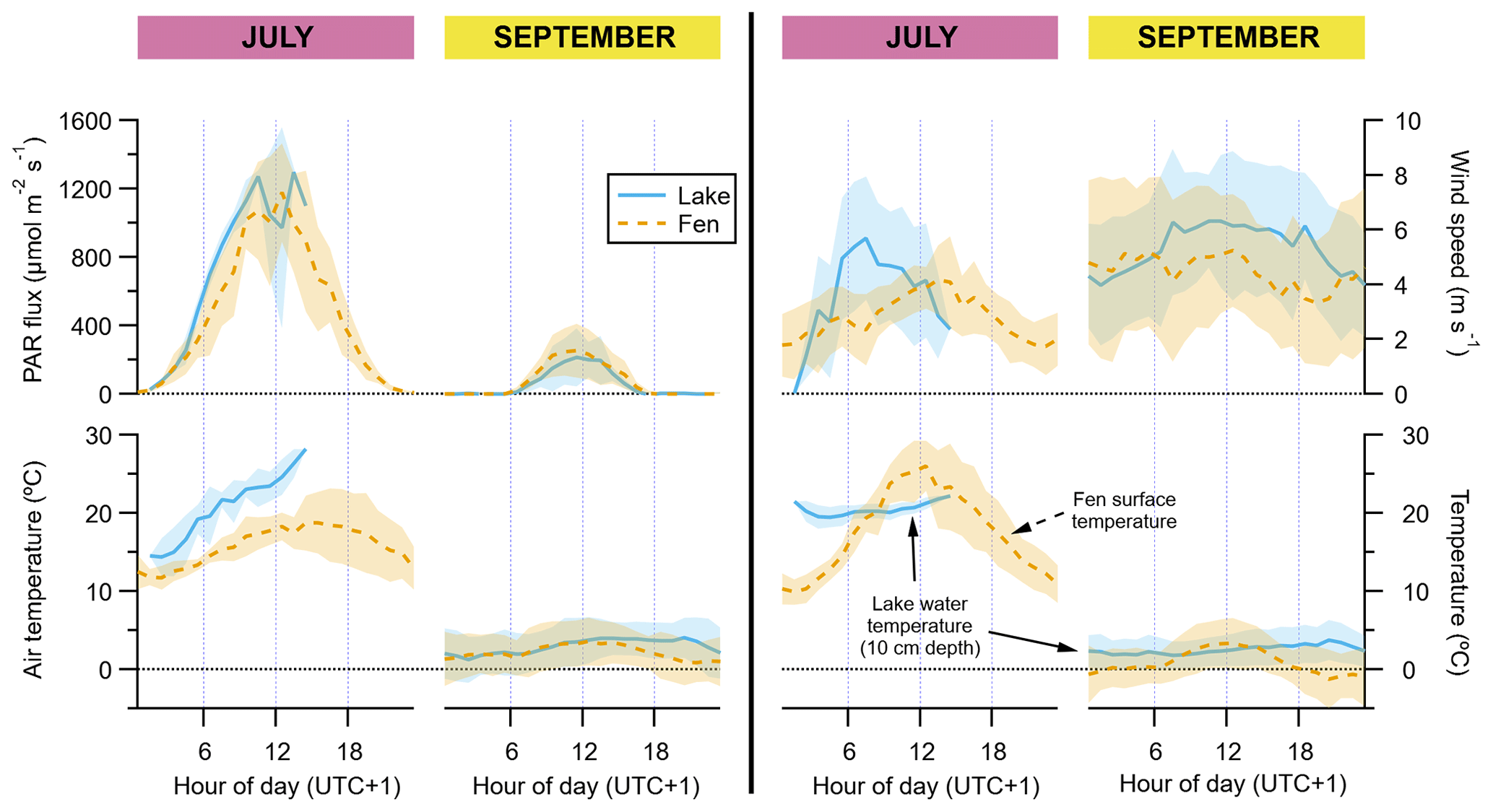
Figure 2Diel cycles of hourly averages of meteorological data, for July and September and for both the lake (solid blue lines) and the fen (dashed orange lines). The peak of the growing season (July) is on the left subpanel of each graph pair, and the post-growing season (September) is on the right subpanel, as indicated on top of the panels. Shaded areas represent ±1 standard deviation. Each vertical axis has a different scaling, but all of them feature a horizontal dotted line showing where the value zero is located.
3.2 Fen VOC fluxes
In July, the fen was a net source of methanol, acetaldehyde, acetone, DMS, isoprene, and monoterpenes (Table 1), with a clear dominance of isoprene (93±22 µmol m−2 d−1 on average ± standard error of the mean). These VOCs showed a typical diurnal cycle with maximum emission around midday (Fig. 3). In September, fen emissions of methanol, isoprene, and monoterpenes were drastically reduced, reaching mean net emissions of 1 µmol m−2 d−1 or less, and none of them followed a discernible diel pattern. Acetaldehyde, acetone, and DMS, in contrast, were deposited to the fen ecosystem with net average rates of , , and µmol m−2 d−1, respectively (Table 1). Thus, acetaldehyde and acetone deposition represented the bulk of VOC flux in the fen after the growing season.
Table 1Average (± standard error of the mean) daily net exchange rates (µmol m−2 d−1) of VOCs, CO2, H2O, and CH4. Negative values represent net deposition or uptake by the ecosystem, and positive values represent net emission. These daily averages were calculated from the hourly averages shown in Figs. 3 and 4.
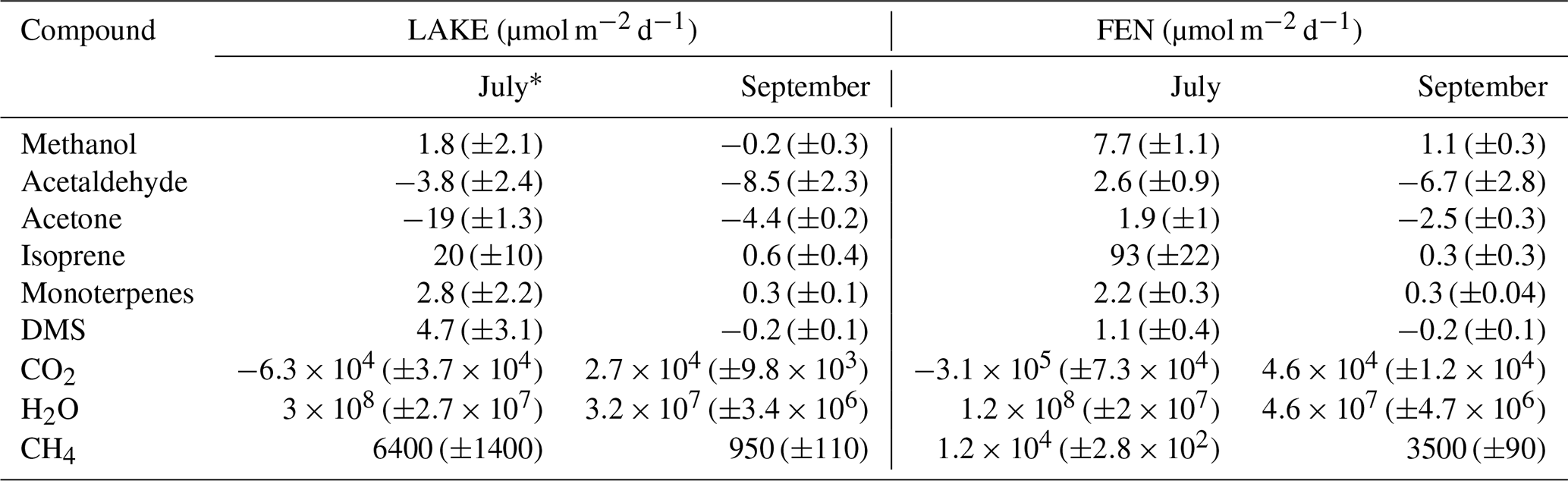
* Based on a limited dataset from 03:00 to 14:00 (UTC + 1).
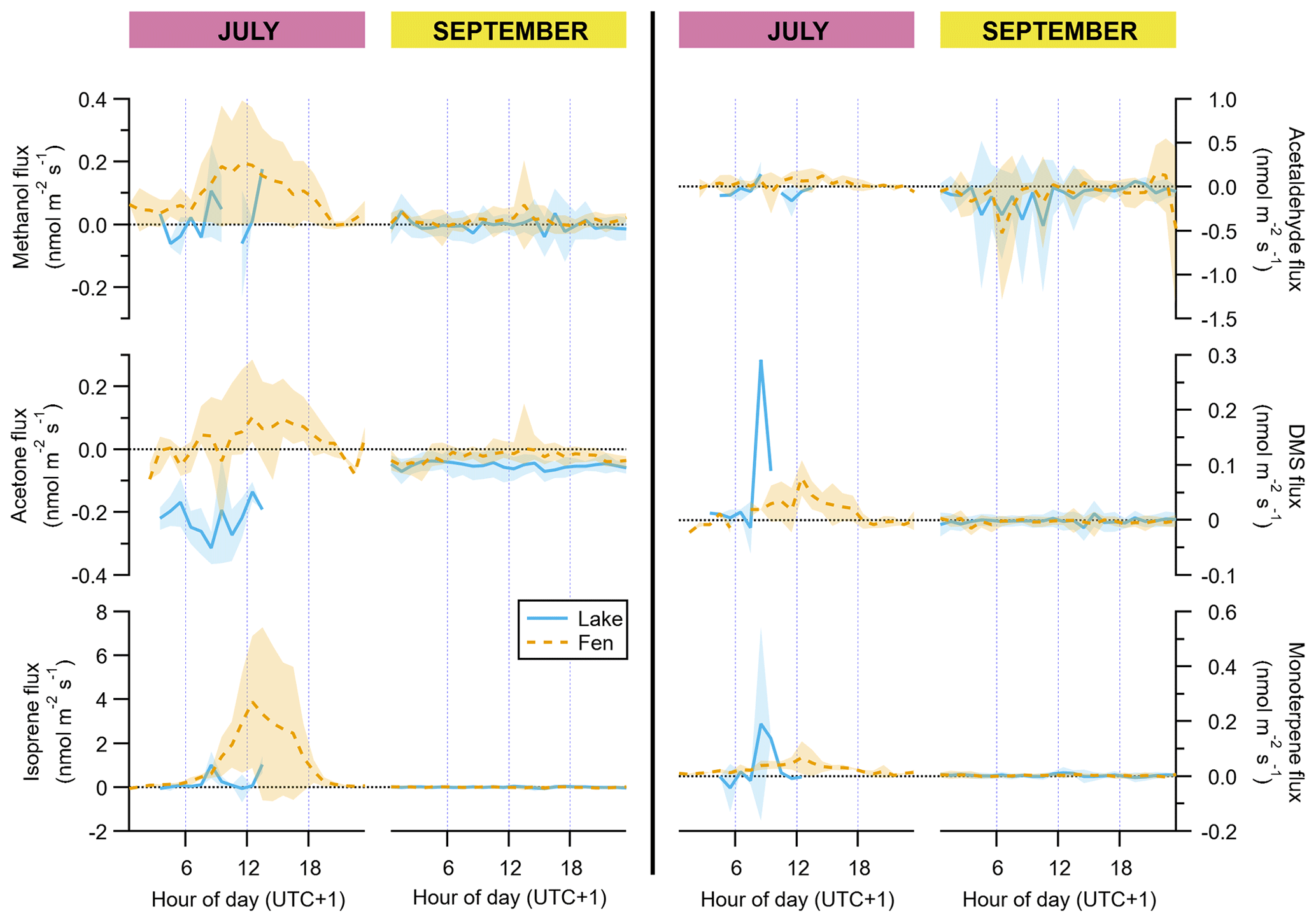
Figure 3Diel cycles of hourly averages of VOC fluxes, for July and September and for both the lake (solid blue lines) and the fen (dashed orange lines). The peak of the growing season (July) is on the left subpanel of each graph pair, and the post-growing season (September) is on the right subpanel, as indicated on top of the panels. Shaded areas represent ±1 standard deviation. Each vertical axis has a different scaling, but all of them feature a horizontal dotted line showing where the value zero is located.
Several biogenic VOC studies in recent years have revealed that isoprene is the major compound in VOC emissions of many arctic and subarctic ecosystems (Holst et al., 2010; Potosnak et al., 2013; Tiiva et al., 2007), including leaf-level measurements of two of the dominant sedge species of our fen: C. rostrata and E. angustifolium (Ekberg et al., 2009). Only two studies, though, measured the ecosystem-scale emissions with EC, one nearby in the Stordalen mire fen and the other in an Alaskan moist acidic tundra (Holst et al., 2010; Potosnak et al., 2013). They published maximum hourly isoprene fluxes that were in the range of 1 to 5.5 nmol m−2 s−1 at the peak of the growing season, comparable in magnitude to our July fen measurements (Fig. 3). A third study that relied on micrometeorology (relaxed eddy accumulation, in this case) was carried out at a boreal fen in southern Finland dominated by Sphagnum spp. mosses. The summer isoprene emissions there were also comparable to our results, with daily average emissions in the range of 35–88 µmol m−2 d−1 (Haapanala et al., 2006).
Most of the other published studies derived ecosystem-scale isoprene fluxes with measurement chambers attached to the ground, enclosing the vegetation and the soil surface together. Pioneering VOC work started in boreal Sphagnum fens of Sweden and Finland with static chambers, finding isoprene fluxes of up to 9 nmol m−2 s−1, which is in range with our measurements (Janson et al., 1999; Janson and De Serves, 1998). At a subarctic fen dominated by Eriophorum spp. and located close to our site in the same Stordalen mire complex, Bäckstrand et al. (2008) measured semi-continuously with automatic chambers and found average total non-methane volatile organic compound (NMVOC) fluxes of 18.5 mgC m−2 d−1. Assuming most of the NMVOCs were isoprene, this would equal 309 µmol m−2 d−1, which is approximately 3 times our result (Table 1). Several other push–pull chamber studies have published results from manipulative experiments, and, in most cases, the non-manipulated control plots showed substantially lower isoprene emissions than the EC and chamber studies mentioned above. For instance, emissions in a Finnish subarctic peatland dominated by the moss Warnstorfia exannulata and the sedges Eriophorum russeolum and Carex limosa were in general at least 1 order of magnitude lower than ours but showed great year-to-year variation with some higher fluxes measured as well (Faubert et al., 2010b; Tiiva et al., 2007). At a fen in Greenland, dominated by the graminoids Carex rariflora and E. angustifolium, isoprene emissions were also at least 1 order of magnitude smaller than our results (Lindwall et al., 2016b). At an experimental site in a heath near Abisko, dominated by evergreen and deciduous dwarf shrubs, graminoids, and forbs and with soil covered by Sphagnum warnstorfii, the average isoprene fluxes were 1 or 2 orders of magnitude lower than ours as well (Tiiva et al., 2008; Valolahti et al., 2015).
Research on isoprene emissions from plant leaves has established that the instantaneous isoprene emission rate depends on the short-term (seconds to hours) light and temperature conditions (Monson et al., 2012). To assess the relative contribution of light and temperature in controlling the isoprene emissions measured at the fen, we used the light (CL) and temperature (CT) activity factors of the G93 empirical leaf-level isoprene emission model (Guenther et al., 1993). We applied the G93 model to our ecosystem-level emissions assuming that the fen vegetation is a single big leaf (e.g. Geron et al., 1997; Seco et al., 2015, 2017). In addition, with the G93 model we could also estimate the standard isoprene emission potential of the fen (at standard conditions: 1000 µmol m−2 s−1 of PAR and surface temperature of 30 ∘C), which was 5.8±0.13 nmol m−2 s−1 (Fig. S5), almost double that calculated for a boreal Sphagnum-dominated fen in southern Finland (Haapanala et al., 2006). The evaluation of the relative contribution of light and temperature to the control of isoprene emissions revealed that, even though light is required for isoprene biosynthesis and subsequent emission, CL did not play a prominent role in driving the short-term variations of the isoprene fluxes, and most of the actual emission regulation was in response to temperature (Fig. S5). However, our highest isoprene fluxes did not follow the expected CT temperature relationship and fell above the regression line (Fig. S5), suggesting a stronger response of our highest isoprene fluxes to temperature. The CT algorithm defines an exponential increase in isoprene emission with temperature until it reaches a maximum at an optimal temperature (35 to 40 ∘C), and beyond that emission decays when denaturation of enzymes occurs (Guenther et al., 1993). At the relatively low temperatures of the Stordalen mire, where vegetation surface temperatures exceed 35 ∘C just on three half-hour periods during our campaign, only the increasing part of the response described by CT was observable. We thus fitted an exponential relationship between our measured isoprene flux and both the air and surface temperatures and calculated their respective Q10 temperature coefficients (Fig. 5). In this case, the Q10 coefficient represents the factor by which isoprene emission increases for every 10∘ rise in temperature. The Q10 of the G93 CT activity factor is 3.3, comparable to similar biogenic VOC emission models with Q10 values between 3 and 6 (Peñuelas and Staudt, 2010). These values over 3 are an indication of the synergy, as temperature rises, between the metabolic processes underlying isoprene emissions, namely isoprene synthase activity and availability of its substrate dimethylallyl diphosphate, that each have Q10≈2 like biochemical reactions in general (Sharkey and Monson, 2014). For our calculation, we used only emission data points for which light was not a limiting factor (i.e. PAR ≥ 1000 µmol m−2 s−1) to avoid interference from the correlation between light and temperature when fitting the temperature response. The Q10 of isoprene emission in response to vegetation surface temperature was 14.5, and the Q10 in response to air temperature was much higher, 131 (Fig. 5). Including in our calculation emission data points measured at PAR ≥ 800 µmol m−2 s−1 increased the number of data points involved (from 52 to 66 at PAR ≥ 1000 and ≥ 800 µmol m−2 s−1, respectively) at the expense of potential light-response interference, although according to the G93 model the light-response effect would be small (CL>0.96 at PAR = 800 µmol m−2 s−1). The lower-PAR Q10 for the surface temperature was 10.3, still above the range 3–6 of the G93 and other biogenic models. The Q10 for the air temperature was 18.6, much lower than for the higher PAR, probably due to the less direct relationship of isoprene emissions with air temperature. Altogether, these calculations suggest a robust, strong response of isoprene fluxes to temperature.
Summarizing the results from an experimentally warmed site, Tang et al. (2016) calculated the isoprene emission temperature response of a subarctic permafrost-free heath ecosystem in Abisko using an Arrhenius-type exponential algorithm, obtaining a Q10 coefficient of 10. Kramshøj et al. (2016) performed similar warming experiments at a dry Arctic tundra heath in Greenland, obtaining a Q10 of 22. These two Q10 coefficients are higher than that of the CT algorithm (Q10=3.3) and closer to our result using the vegetation surface temperature (Q10=14.5; red squares in Fig. 5). Both studies used air temperature inside the chambers for their calculations, which is typically higher than the ambient air temperature, considering that the combined effect of solar radiation and limited air circulation normally heats up the inside of the chambers. Details about where the temperature is measured – temperature that later is used to derive temperature responses – can be important because Arctic vegetation exhibits a large discrepancy between its surface temperature and that of the air. For example, the vegetation surface was on average 8 ∘C, and up to 21 ∘C, warmer than the air at a heath in Greenland (Lindwall et al., 2016a), which coincides with our Stordalen temperature readings (Figs. 2, 5). Indeed, the response of our isoprene emissions to air temperature was even steeper (Q10=131; blue triangles in Fig. 5) than to surface temperature. At the same Stordalen wetland as our study, Holst et al. (2010) found a steep temperature response to air temperatures above 15 ∘C, in agreement with our results (Fig. 5) and previous high-latitude studies (Kramshøj et al., 2016; Lindwall et al., 2016a, b; Rinnan et al., 2014). Hence, our high Q10 values corroborate that Arctic vegetation can have a stronger temperature sensitivity compared to plants from lower latitudes, which underpin the most used biogenic emission models (Guenther et al., 2006).
There are few accounts of non-isoprene fluxes from subarctic wetland ecosystems. Monoterpene emissions from chamber experiments in an Abisko heath showed great variability: sometimes in the range of our fen measurements (we found average hourly maximum of 0.06 nmol m−2 s−1; Fig. 3) while sometimes 1 order of magnitude lower (Faubert et al., 2010a; Valolahti et al., 2015). Even lower (3 orders of magnitude) were the monoterpene fluxes from a subarctic fen in Finland (Faubert et al., 2010b), while a boreal Sphagnum fen in Finland had comparable or higher fluxes (averages between 0.05 and 0.2 nmol m−2 s−1) than our subarctic fen (Janson et al., 1999).
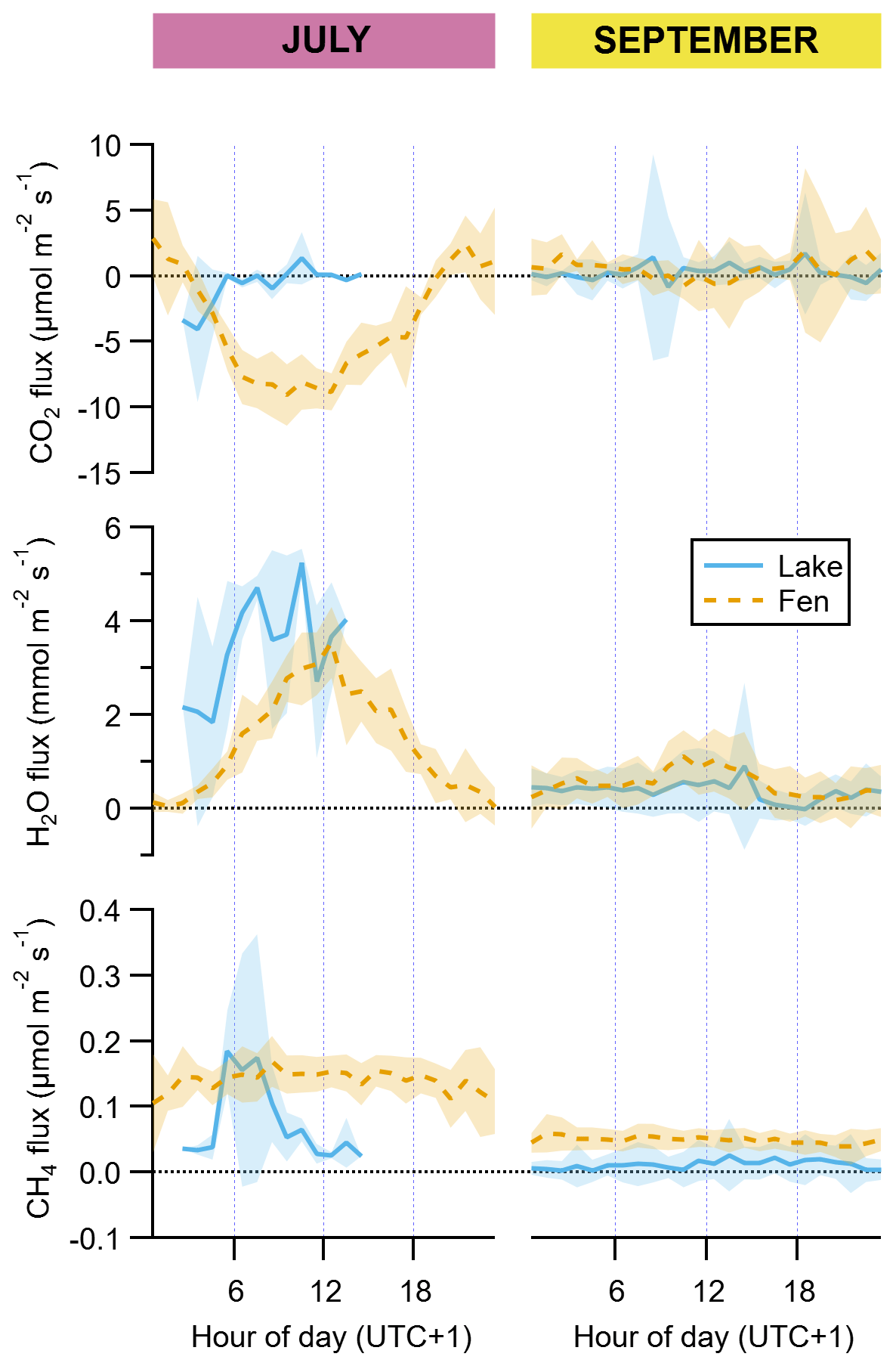
Figure 4Diel cycles of hourly averages of fluxes of CO2, H2O, and CH4 for July and September and for both the lake (solid blue lines) and the fen (dashed orange lines). The peak of the growing season (July) is on the left subpanel of each graph pair, and the post-growing season (September) is on the right subpanel, as indicated on top of the panels. Shaded areas represent ±1 standard deviation. Each vertical axis has a different scaling, but all of them feature a horizontal dotted line showing where the value zero is located.
Regarding methanol, EC fluxes investigated at the Stordalen mire wetland by Holst et al. (2010) reached a noontime average hourly maximum of 1.3 nmol m−2 s−1 in early August, which is higher than our 0.2 nmol m−2 s−1 in July (Fig. 3). They measured net methanol deposition clearly at night, whereas we observed a net zero flux at the end of the day (Fig. 3). Deposition of methanol to vegetation during nighttime has been linked to dissolution into dew droplets because methanol is highly soluble in water (Seco et al., 2007). At our site, the wet surface of the fen could potentially play an important role, but our data do not show any significant methanol deposition. The net methanol fluxes observed at our subarctic fen in July are lower than most of the published methanol fluxes from a diverse array of ecosystem-scale studies, which also confirmed the widespread importance of methanol deposition (Seco et al., 2007; Wohlfahrt et al., 2015). Acetaldehyde and acetone net emissions in July were also smaller than other published fluxes from terrestrial vegetation (Seco et al., 2007), and in September they were mainly deposited. DMS showed the same behaviour as methanol, with mainly emission in July and deposition after the growing season (Fig. 3).
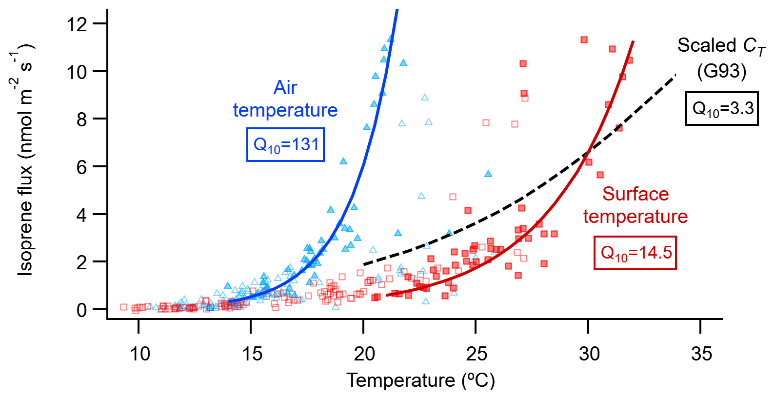
Figure 5Relationship of the isoprene flux from the fen with the air temperature (blue triangles) measured at 2 m height on the EC mast, and with the vegetation surface temperature (red squares) measured at the nearby ICOS station. The data points shown are all the July 30 min fluxes that passed the EC quality criteria (n=161; open and closed symbols). Solid lines show the exponential equation , where F0 is the isoprene flux rate at temperature T0 (= 0 ∘C), F is the flux rate at temperature T (∘C), and Q10 is the temperature coefficient. F0 and Q10 were calculated by fitting the data to the linear equation , where a0 is the intercept at T=0 ∘C. For the fit, only fluxes not limited by light (when PAR was 1000 µmol m−2 s−1 or more; n=52; closed symbols) were binned into 1∘ bins (not shown). Then the average fluxes of the bins, excluding bins containing a single flux value, were used to perform an orthogonal distance regression weighed by the standard deviation of each bin average. As a reference, the dashed black line shows the relationship with leaf temperature of the temperature activity factor (CT) of the G93 model (Guenther et al., 1993), scaled to coincide with the surface temperature fit at 30 ∘C.
All these non-isoprenoid VOCs followed a diffuse relationship with temperature and/or light (Fig. S3), reflecting the complex nature of the controls over their fluxes at the ecosystem level (Seco et al., 2007). DMS can be emitted by plants (Fall et al., 1988; Geng and Mu, 2006; Jardine et al., 2010) and also, driven by temperature, from soils (Staubes et al., 1989; Yang et al., 1996). Methanol can be emitted constitutively by plants throughout their growing season, with increased release linked to leaf expansion (Aalto et al., 2014; Hüve et al., 2007) and emission bursts elicited by herbivore feeding (Peñuelas et al., 2005a). Methanol emissions have also been associated with soils. For example, methanol was one of the main compounds released from subalpine forest floor (Gray et al., 2014) and thawing permafrost (Kramshøj et al., 2018). Acetaldehyde is produced in flooded roots (Fall, 2003), which is potentially an important source in a waterlogged fen for species not adapted to this growth condition, like shrubs. The graminoids, in contrast, transport air down to their roots through a specialized tissue in their leaves and stems, and they do not suffer from anoxia (Schütz et al., 1991). The exchange of acetone, acetaldehyde, and methanol between plants and the atmosphere is controlled by the stomatal conductance due to their water solubility, and, furthermore, their atmospheric mixing ratios can have influence on the fluxes to some extent (Filella et al., 2009; Jardine et al., 2008; Niinemets and Reichstein, 2003; Seco et al., 2007). In addition, the peat and its microbial communities are also a potential source and sink for many volatiles that can be exchanged between the soil and the atmosphere from many biogeochemical processes (Albers et al., 2018; Kramshøj et al., 2018; Woodcroft et al., 2018).
Lastly, our analytical system did not capture any sesquiterpene fluxes. We know from chamber measurements that vegetation present at the Stordalen mire emits sesquiterpenes. For example, the mountain birch (B. pubescens var. pumila), which covers an area of almost 600 000 ha in the Scandinavian subarctic, can emit important amounts of sesquiterpenes (Haapanala et al., 2009). Other experiments in nearby Abisko heaths, mentioned above, documented sesquiterpene flux rates similar to those of monoterpenes measured in the same study (Faubert et al., 2010a; Valolahti et al., 2015). Most recently, sesquiterpenes have been detected as the main terpenoid emissions after isoprene at a subarctic wetland in Finland (Hellén et al., 2020). One obvious reason for our lack of sesquiterpene signal is that our flux footprint did not include a significant amount of high-emitting species since, for example, most of the nearby birch patches were outside of it. Equally important is the fact that, due to their high reactivity, sesquiterpenes are lost through fast chemical reactions and through interactions with our long inlet tubing wall, so presumably they never made it to our PTR-TOF-MS to be detected. Therefore, the measurement of ecosystem-wide fluxes of sesquiterpenes with EC remains a challenge for future field campaigns.
3.3 Lake VOC fluxes
The number of available lake half-hour fluxes in July was low (n≈20) due to technical issues, wind direction partitioning, and fluxes discarded by EC quality assurance criteria. These reasons and the consequent lack of data for half of the hours of the average day (Fig. 3) justify that we consider these results exploratory. In particular, compounds such as DMS and monoterpenes had mean daily fluxes dominated by one or two hourly average data points that were not actually hourly averages, since they were based on only one measurement during that hour (i.e. data points without standard deviation shading in Fig. 3). However, there are so few observations of lake VOC fluxes that it is important that we document the sparse data we have.
VOC fluxes assigned to the lake wind direction could potentially have some influence from the vegetation of the island in the lake, because under certain conditions the edge of the EC tower footprint reached that far. A previous study at this site described CO2 uptake during the day from the lake EC measurements in summertime (Jammet et al., 2017). Such uptake was later interpreted as a result of the photosynthetic activity on the island, since water sampling indicated the surface water of lake Villasjön was consistently supersaturated with respect to atmospheric CO2 (Jansen et al., 2019a). During our week-long July measurements, we only observed lake CO2 uptake in the early morning (Fig. 4) when VOC emissions were small (Fig. 3). Hence, we assume that the vegetation of the island did not substantially bias our lake VOC fluxes although some influence cannot be entirely ruled out.
The most striking feature of the lake ecosystem is that it was a sink for acetaldehyde and acetone in both studied periods (Fig. 3, Table 1). Similar to the fen, the deposition of these compounds accounted for most of the VOC flux in the lake in September. Acetone deposition peaked in July with an average of µmol m−2 d−1, while that of acetaldehyde was highest in September with µmol m−2 d−1 (Table 1). There was a correlation of the acetaldehyde and acetone deposition rates with their corresponding atmospheric mixing ratios (Fig. 6), with increasing deposition at higher mixing ratios, resulting in average deposition velocities of and cm s−1 for acetone and acetaldehyde, respectively. The high water solubility of these short-chain oxygenated VOCs helps their deposition from the air to the water and may partly explain the correlation of the deposition rate with their atmospheric mixing ratios (Fig. 6). The flux of these two carbonyl VOCs showed a relationship to air temperature as well, which might very well be coincidental and dependent on atmospheric mixing ratios. Acetone deposition was more intense at higher air temperatures, in July, when its mixing ratios were also higher (Fig. 6). In contrast to acetone, acetaldehyde did not present a clear relationship with air temperature, but its strongest deposition rates occurred at air temperatures below 3 ∘C, concurrent with higher mixing ratios (Fig. 6).
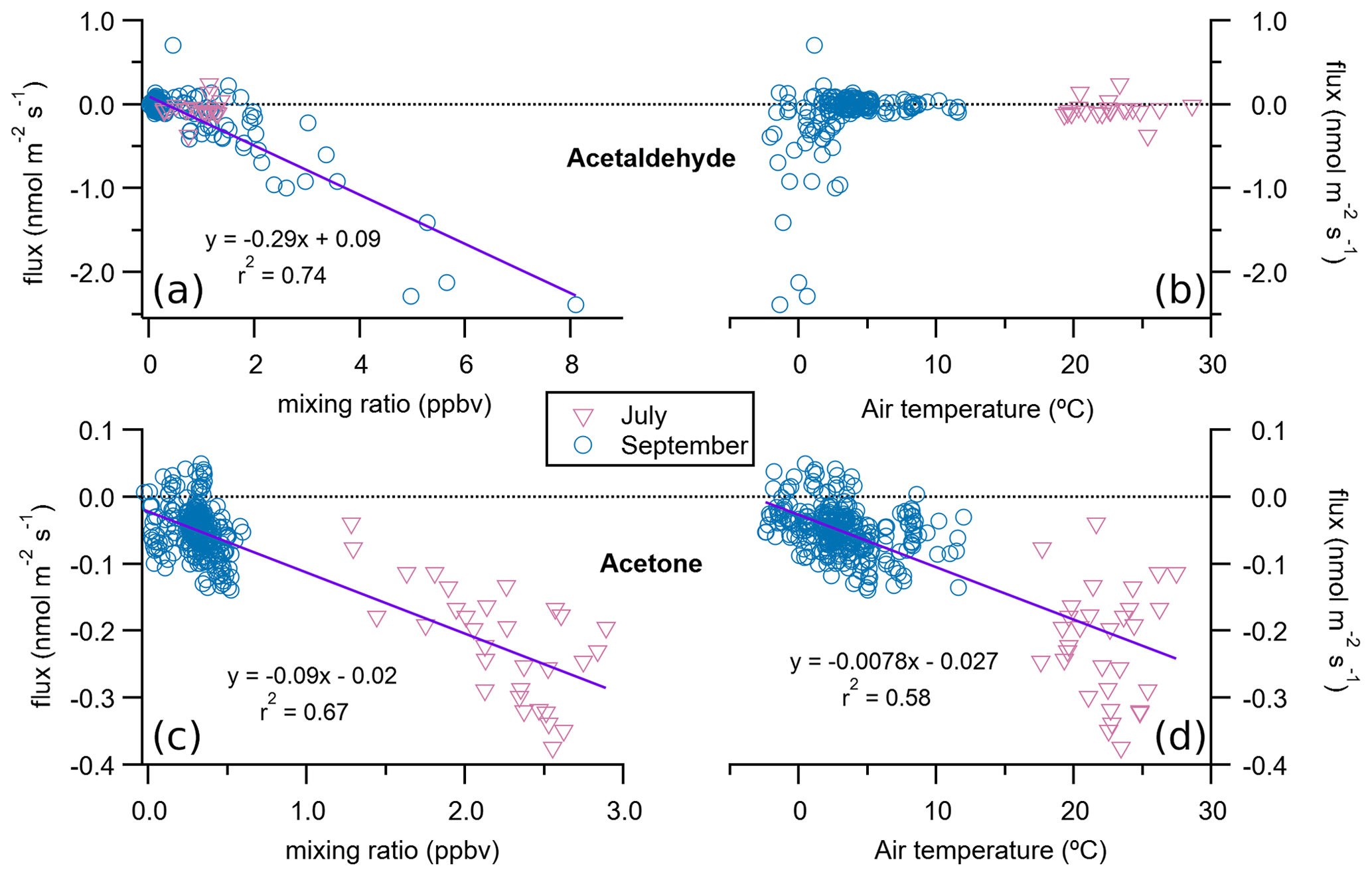
Figure 6Relationship of lake fluxes of acetaldehyde (a, b) and acetone (c, d) with their respective atmospheric mixing ratios (a, c) and the air temperature (b, d). Each solid line and corresponding equation represent an orthogonal distance regression to all 30 min flux data points for both July and September (n=191 for acetaldehyde and n=338 for acetone).
These carbonyl compounds have not only natural sources such as emission from vegetation and soil: they also originate from human activities and from atmospheric degradation of other precursor VOCs (Seco et al., 2007). The limited reactivity of acetone in the troposphere makes it relatively long lived, typically up to 15 d (Singh et al., 2004), which means that the deposited acetone can be advected from far away (Patokoski et al., 2015). We have not found studies in the literature on air–water fluxes of acetaldehyde or acetone in freshwater environments – only a few in marine environments. Yet those marine studies have contradictory results on whether the ocean is a net sink or a source of acetone (Fischer et al., 2012), suggesting a location-dependent behaviour where tropical and productive areas are a net source while high-latitude oligotrophic oceans are either in an air–water equilibrium (i.e. zero net flux) or act as net sinks of acetone (Beale et al., 2013, 2015; Lawson et al., 2020; Marandino, 2005; Schlundt et al., 2017; Taddei et al., 2009; Tanimoto et al., 2014). Villasjön, as an oligotrophic high-latitude lake, would fit in that conceptual framework as a sink of acetone, in agreement with our observations. The direction of the acetaldehyde flux in seawater has been reported to vary along the year during an annual study in UK shelf waters (Beale et al., 2015) and also to be mostly emitted during short-term measurements in a Norwegian fjord mesocosm experiment (Sinha et al., 2007). Further, the lake sink of acetaldehyde and acetone detected with our measurements in the snow-free season may be reversed to a source once the valley is covered in snow, as release of acetaldehyde, acetone, and other carbonyl compounds from snow has been documented (Couch et al., 2000).
Interestingly, even though methanol is more soluble in water than acetone or acetaldehyde (Sander, 2015), its deposition to the lake did not reach the intensity displayed by the two carbonyl compounds (Fig. 3). Instead, average methanol fluxes showed little to no flux, either deposition or emission, along the day during both seasons. Again, given the dearth of published observations, we can only compare our methanol fluxes to marine studies. In contrast to acetone and acetaldehyde and their variable flux direction, methanol has been reported to be consistently deposited to the ocean surface, where it could represent a supply of energy and carbon for marine microbes (Beale et al., 2015; Sinha et al., 2007; Yang et al., 2013).
Like the fen, the lake also emitted isoprene in July, although without a visible diel pattern given the incomplete dataset (Fig. 3). Nevertheless, our available data showed maximum hourly average net emissions of 1 nmol m−2 s−1, and a daily average net rate of 0.24±0.12 nmol m−2 s−1 (equivalent to 20±10 µmol m−2 d−1; Table 1). These numbers are 2 to 3 orders of magnitude higher than isoprene emissions calculated at the large temperate oligotrophic Lake Constance (Germany) in the month of July, with maximum hourly average emission rates of 0.004 nmol m−2 s−1 (Steinke et al., 2018). Based on the data from Lake Constance, Steinke et al. (2018) suggested that Arctic lakes could rival terrestrial vegetation emissions in these zones where lake areal coverage is high and terrestrial isoprene sources are small. Our numbers do not fully support that suggestion for the peak of the season at our site, since the fen net emission was roughly 4.5 times that of the lake (Table 1), although it may hold in zones with a ratio of lake to vegetation coverage over five. For instance, the Stordalen catchment has 4.5 % of lake coverage and 3.9 % of fen coverage (Lundin et al., 2016), so the lake-to-vegetation ratio is 1.2 and much lower if we include other types of vegetation. Still, their suggestion may be valid for other periods. For example, in our case during the senescent period in September, even though the flux magnitudes were much smaller than in July, the lake average isoprene emission was double that of the fen (0.6±0.4 and 0.3±0.3 µmol m−2 d−1, respectively; Table 1). We found no other report of isoprene fluxes from lakes, despite the likely existence of many sources analogous to those known in seawater such as phytoplankton, seaweeds, bacteria, and cyanobacteria (Broadgate et al., 2004; Exton et al., 2013; Fall and Copley, 2000; Shaw et al., 2003, 2010). A number of available publications suggest that ocean waters are sources of isoprene to the atmosphere at rates comparable to those calculated for Lake Constance, i.e. 2 orders of magnitude lower than ours (Broadgate et al., 1997; Kameyama et al., 2014; Li et al., 2017; Sinha et al., 2007).
DMS is a commonly studied marine trace gas because of its role in aerosol and cloud nucleation chemistry (Carpenter et al., 2012), but there are far fewer observations in freshwater environments. As far as we know, no EC measurements of DMS from lakes exist, so the few published studies that report a DMS flux employed alternative techniques to calculate the fluxes, for example using the DMS concentration difference between water and air with an air–water transfer model to calculate the fluxes. DMS emissions calculated by Steinke et al. (2018) for the 252 m deep Lake Constance were, as for isoprene, 2 orders of magnitude smaller (maximum hourly average emission rates of 0.003 nmol m−2 s−1) than our July fluxes. A study in Canadian boreal lakes estimated DMS emissions up to a few µmol m−2 d−1 for shallow lakes, which is on the lower range of the July fluxes in the shallow Villasjön. That study also noted that emissions from deeper lakes were smaller than from shallow or medium-depth lakes (Sharma et al., 1999), while a similar study in the same geographical area found average DMS fluxes of around 1 µmol m−2 d−1 from lakes ranging in depths from 1.5 to 20 m but with a 5 m deep lake showing much higher emissions of up to 4 µmol m−2 d−1 on average (Richards et al., 1991). Other authors measured DMS concentrations in a stratified lake in North America, at different depths down to 13 m, and concluded that DMS fluxes to the atmosphere must have been insignificant given that DMS was not present in surface and near-surface water (Hu et al., 2007). Another study took a different approach and utilized the phytoplankton biomass and its content of DMS precursors in lake Kinneret (Israel) to estimate an average DMS emission of 3.3 µmol m−2 d−1 (Ginzburg et al., 1998), similar to our July average of 4.7±3.1 µmol m−2 d−1 (Table 1). In contrast, DMS fluxes from the ocean have been directly measured by EC in different places around the globe, with reported emissions as high as 97 µmol m−2 d−1 (Bell et al., 2013; Marandino et al., 2007, 2009; Smith et al., 2018), even up to 300 µmol m−2 d−1 during a unicellular phytoplankton bloom (Marandino et al., 2008), but in many cases with average emissions in the same range as our lake July average flux (Huebert et al., 2004; Tanimoto et al., 2014; Yang et al., 2011a, b).
3.4 CO2, CH4, and H2O fluxes
The fluxes of CO2 and CH4 (as well as H2O) were not the focus of this study, and, moreover, their temporal patterns and environmental drivers over several years at the same site have been examined in detail elsewhere (Jammet et al., 2015, 2017; Jansen et al., 2019a, 2020). Here, we mainly included them to contextualize the VOC fluxes and thus provide a broader overview of the trace gas exchange of our fen and Villasjön during our two measurement periods. Furthermore, as in the case of the July VOC fluxes, the limited data availability from the lake in July (36 and 51 half-hourly fluxes for CO2 and CH4, respectively) advises the consideration of the presented lake trace gas exchanges with prudence.
Net molar fluxes of CO2, CH4, and H2O were at least 2, and up to 7, orders of magnitude higher than the VOC fluxes (Table 1). Water vapour and CH4 showed net average daily emission in both the lake and the fen and during both periods, while CO2 showed net uptake in July and net release in September, in both the lake and the fen (Table 1).
Uptake of CO2 and evapotranspiration in the fen followed a well-defined diel cycle likely due to the physiological activity of the vegetated surface, with maxima around noontime, notably in July (Fig. 4). In September, a similar pattern was apparent in the fen's diel cycles (Fig. 4), but the magnitude of the daytime fluxes was much smaller. It was so much smaller that the weaker CO2 uptake during daylight hours did not compensate for the CO2 release during the rest of the day, resulting in a 24 h aggregate mean flux that represented a net release of CO2 to the atmosphere from the fen (Table 1). CH4 emissions from the fen in July were on average 3.5 times higher than in September (Table 1), and their diel emission cycle showed an overall flat pattern in both periods (Fig. 4).
The lake was a net sink of CO2 in July, especially due to stronger uptake during the early hours of the day, and a net source in September, during which there was no diel cycle (Table 1, Fig. 4). Evaporation from the lake was approximately 10-fold higher in July than in September on a 24 h basis, and compared to the evapotranspiration from the fen, it was higher in July as well (Table 1, Fig. 4). Daily CH4 emissions from the lake were smaller than from the fen during both periods (Table 1).
A comparison of the VOC carbon fluxes with the fluxes in the form of CO2 and CH4 (Table 1) reveals that the average net VOC emission of the fen in July, summing the six VOC species reported in this paper, represented 0.16 % of the fen net carbon uptake as CO2 (of which isoprene alone was 0.15 %) and 4.2 % of the net carbon release as CH4 (isoprene alone, 3.9 %). In September, the absolute VOC net carbon flux at the fen, i.e. the total net amount of carbon exchanged in the form of VOCs, including both the VOCs with net emission and those with net uptake, added up 0.06 % of the net CO2 carbon and 0.76 % of the net CH4 carbon emitted from the fen.
The same comparison for the lake (Table 1) shows that the aggregate absolute VOC net exchange amounts to 0.32 % of the CO2 and 3.2 % of the CH4 net carbon fluxes of the lake. In September, the absolute VOC net carbon flux in the lake was equivalent to 0.13 % of the net CO2 carbon release flux and 3.8 % of the net CH4 carbon emission flux.
Here we presented an eddy covariance dataset measured from two distinct common subarctic landscape types: a permafrost-free fen and a shallow post-glacial lake. Isoprene dominated by far the VOC fluxes from the fen at the peak of the season, while after the growing season the fen was characterized by deposition of acetaldehyde and acetone (Fig. 3, Table 1). Furthermore, the isoprene emissions from the fen in July were strongly stimulated by temperature and, in agreement with previous arctic and subarctic VOC measurements (Holst et al., 2010; Tang et al., 2016), exhibited a higher temperature sensitivity (Q10=14.5) than described by the temperature response curves typically used in biogenic emission models (), which are based on measurements made in lower latitudes (Guenther et al., 2006). Our measurements also displayed the disparity between the temperature of the air and that of the vegetation surface, with the latter being several degrees warmer during daytime (Figs. 2 and 5). Consequently, it is advisable that future VOC studies measure accurately and precisely the vegetation temperatures that represent the thermal conditions controlling the VOC production and release processes. Furthermore, while we do not suggest taking these Q10 values as true coefficients to be directly implemented into modelling, it is worth mentioning that care should be taken when applying Q10 values in models. Otherwise, a mismatch could translate into erroneous results, for instance when using a Q10 derived from the response to air temperature in models that drive VOC emissions with leaf temperature and vice versa.
Our lake VOC fluxes can be considered exploratory due to the low amount of data available. Despite this, they are valuable given the lack of observations of freshwater fluxes. We showed that the lake was a sink of acetone and acetaldehyde in both July and September, with average deposition velocities of and cm s−1 for acetone and acetaldehyde, respectively (Figs. 3, 6, Table 1).
The carbon exchanged as VOC net fluxes from both fen and lake constituted less than 0.5 % and less than 5 % of the CO2 and CH4 net carbon ecosystem exchange, respectively. These low proportions are probably one of the reasons, together with technical and logistical challenges (Rinne et al., 2016), of the limited amount of existing VOC studies in lakes or high-latitude ecosystems. However, technological advances are gradually removing practical obstacles, and, in addition, growing concern about climate change repercussions warrants more research in this rapidly warming area of the world, especially given the importance of VOCs as precursors for aerosols (Paasonen et al., 2013; Svenningsson et al., 2008). CO2 and CH4 fluxes are already under intense investigation to quantify the strength of their sinks and sources (e.g. Jeong et al., 2018; Oh et al., 2020). Recently, arctic VOCs have received increased attention (e.g. Kramshøj et al., 2016, 2018, 2019), and this study is another contribution towards the understanding of VOC budgets in northern wetlands and inland waters.
VOC flux data used in this article, together with PAR, air temperature, and vegetation surface temperature, are available for download at https://doi.org/10.5281/zenodo.3886457 (Seco et al., 2020). CO2, H2O, and CH4 fluxes and wind direction and speed can be downloaded from http://www.icos-etc.eu/home/site-details?id=SE-St1 (Jansen et al., 2019b). Villasjön water temperatures are available at https://doi.org/10.17043/stordalen-lake-temperature-3 (Crill et al., 2020).
The supplement related to this article is available online at: https://doi.org/10.5194/acp-20-13399-2020-supplement.
RS, TH, MSM, AWN, TL, TS, and JJ performed measurements and contributed data. RR conceptualized and supervised the study and acquired funding to support this research. RS analysed the data and wrote the original draft. All authors contributed to manuscript writing and revision and read and approved the submitted version.
The authors declare that they have no conflict of interest.
We are grateful to ICOS Sweden and the Abisko Scientific Research Station for providing excellent logistics for the work. ICOS Sweden is co-funded by the Swedish Research Council.
This research has been supported by the European Research Council (TUVOLU – Tundra biogenic volatile emissions in the 21st century, grant no. 771012) and the Marie Skłodowska-Curie actions (HIVOL, grant no. 751684) under the European Union's Horizon 2020 research and innovation programme, the Independent Research Fund Denmark | Natural Sciences, the Swedish Research Council (grant no. 2013-5562), the European Commission under the Seventh Framework Programme (PAGE21, grant no. 282700), and by the Danish National Research Foundation (CENPERM DNRF100).
This paper was edited by Thomas Karl and reviewed by Juho Aalto and one anonymous referee.
Aalto, J., Kolari, P., Hari, P., Kerminen, V.-M., Schiestl-Aalto, P., Aaltonen, H., Levula, J., Siivola, E., Kulmala, M., and Bäck, J.: New foliage growth is a significant, unaccounted source for volatiles in boreal evergreen forests, Biogeosciences, 11, 1331–1344, https://doi.org/10.5194/bg-11-1331-2014, 2014.
Albers, C. N., Kramshøj, M., and Rinnan, R.: Rapid mineralization of biogenic volatile organic compounds in temperate and Arctic soils, Biogeosciences, 15, 3591–3601, https://doi.org/10.5194/bg-15-3591-2018, 2018.
Atkinson, R.: Atmospheric chemistry of VOCs and NOx, Atmos. Environ., 34, 2063–2101, https://doi.org/10.1016/S1352-2310(99)00460-4, 2000.
Aubinet, M., Chermanne, B., Vandenhaute, M., Longdoz, B., Yernaux, M., and Laitat, E.: Long term carbon dioxide exchange above a mixed forest in the Belgian Ardennes, Agr. Forest Meteorol., 108, 293–315, https://doi.org/10.1016/S0168-1923(01)00244-1, 2001.
Bäckstrand, K., Crill, P. M., Mastepanov, M., Christensen, T. R., and Bastviken, D.: Non-methane volatile organic compound flux from a subarctic mire in Northern Sweden, Tellus B, 60, 226–237, https://doi.org/10.1111/j.1600-0889.2007.00331.x, 2008.
Baldwin, I. T., Halitschke, R., Paschold, A., von Dahl, C. C., and Preston, C. A.: Volatile signaling in plant-plant interactions: “Talking trees” in the genomics era, Science, 311, 812–815, https://doi.org/10.1126/science.1118446, 2006.
Beale, R., Dixon, J. L., Arnold, S. R., Liss, P. S., and Nightingale, P. D.: Methanol, acetaldehyde, and acetone in the surface waters of the Atlantic Ocean, J. Geophys. Res.-Ocean., 118, 5412–5425, https://doi.org/10.1002/jgrc.20322, 2013.
Beale, R., Dixon, J. L., Smyth, T. J., and Nightingale, P. D.: Annual study of oxygenated volatile organic compounds in UK shelf waters, Mar. Chem., 171, 96–106, https://doi.org/10.1016/j.marchem.2015.02.013, 2015.
Bell, T. G., De Bruyn, W., Miller, S. D., Ward, B., Christensen, K. H., and Saltzman, E. S.: Air–sea dimethylsulfide (DMS) gas transfer in the North Atlantic: evidence for limited interfacial gas exchange at high wind speed, Atmos. Chem. Phys., 13, 11073–11087, https://doi.org/10.5194/acp-13-11073-2013, 2013.
Broadgate, W., Malin, G., Küpper, F., Thompson, A., and Liss, P.: Isoprene and other non-methane hydrocarbons from seaweeds: a source of reactive hydrocarbons to the atmosphere, Mar. Chem., 88, 61–73, https://doi.org/10.1016/j.marchem.2004.03.002, 2004.
Broadgate, W. J., Liss, P. S., and Penkett, S. A.: Seasonal emissions of isoprene and other reactive hydrocarbon gases from the ocean, Geophys. Res. Lett., 24, 2675–2678, https://doi.org/10.1029/97GL02736, 1997.
Buras, A., Rammig, A., and Zang, C. S.: Quantifying impacts of the 2018 drought on European ecosystems in comparison to 2003, Biogeosciences, 17, 1655–1672, https://doi.org/10.5194/bg-17-1655-2020, 2020.
Callaghan, T. V., Bergholm, F., Christensen, T. R., Jonasson, C., Kokfelt, U., and Johansson, M.: A new climate era in the sub-Arctic: Accelerating climate changes and multiple impacts, Geophys. Res. Lett., 37, L14705, https://doi.org/10.1029/2009GL042064, 2010.
Carpenter, L. J., Archer, S. D., and Beale, R.: Ocean-atmosphere trace gas exchange, Chem. Soc. Rev., 41, 6473, https://doi.org/10.1039/c2cs35121h, 2012.
Couch, T. L., Sumner, A. L., Dassau, T. M., Shepson, P. B., and Honrath, R. E.: An investigation of the interaction of carbonyl compounds with the snowpack, Geophys. Res. Lett., 27, 2241–2244, https://doi.org/10.1029/1999GL011288, 2000.
Crill, P., Wik, M., and Jansen, J.: Temperatures in subarctic lakes on the Stordalen Mire, Abisko, Northern Sweden, Dataset version 3.0, Bolin Centre Database, https://doi.org/10.17043/stordalen-lake-temperature-3, 2020.
Ekberg, A., Arneth, A., Hakola, H., Hayward, S., and Holst, T.: Isoprene emission from wetland sedges, Biogeosciences, 6, 601–613, https://doi.org/10.5194/bg-6-601-2009, 2009.
Exton, D. A., Suggett, D. J., McGenity, T. J., and Steinke, M.: Chlorophyll-normalized isoprene production in laboratory cultures of marine microalgae and implications for global models, Limnol. Oceanogr., 58, 1301–1311, https://doi.org/10.4319/lo.2013.58.4.1301, 2013.
Fall, R.: Abundant oxygenates in the atmosphere: A biochemical perspective, Chem. Rev., 103, 4941–4951, 2003.
Fall, R. and Copley, S. D.: Bacterial sources and sinks of isoprene, a reactive atmospheric hydrocarbon, Environ. Microbiol., 2, 123–130, https://doi.org/10.1046/j.1462-2920.2000.00095.x, 2000.
Fall, R., Albritton, D. L., Fehsenfeld, F. C., Kuster, W. C., and Goldan, P. D.: Laboratory studies of some environmental variables controlling sulfur emissions from plants, J. Atmos. Chem., 6, 341–362, https://doi.org/10.1007/BF00051596, 1988.
Faubert, P., Tiiva, P., Rinnan, Å., Michelsen, A., Holopainen, J. K., and Rinnan, R.: Doubled volatile organic compound emissions from subarctic tundra under simulated climate warming, New Phytol., 187, 199–208, https://doi.org/10.1111/j.1469-8137.2010.03270.x, 2010a.
Faubert, P., Tiiva, P., Rinnan, Å., Räsänen, J., Holopainen, J. K., Holopainen, T., Kyrö, E., and Rinnan, R.: Non-Methane Biogenic Volatile Organic Compound Emissions from a Subarctic Peatland Under Enhanced UV-B Radiation, Ecosystems, 13, 860–873, https://doi.org/10.1007/s10021-010-9362-1, 2010b.
Filella, I., Peñuelas, J., and Seco, R.: Short-chained oxygenated VOC emissions in Pinus halepensis in response to changes in water availability, Acta Physiol. Plant., 31, 311–318, https://doi.org/10.1007/s11738-008-0235-6, 2009.
Filella, I., Primante, C., Llusià, J., Martín González, A. M., Seco, R., Farré-Armengol, G., Rodrigo, A., Bosch, J., and Peñuelas, J.: Floral advertisement scent in a changing plant-pollinators market, Sci. Rep.-UK, 3, 3434, https://doi.org/10.1038/srep03434, 2013.
Fischer, E. V., Jacob, D. J., Millet, D. B., Yantosca, R. M., and Mao, J.: The role of the ocean in the global atmospheric budget of acetone, Geophys. Res. Lett., 39, L01807, https://doi.org/10.1029/2011GL050086, 2012.
Foken, T., Göockede, M., Mauder, M., Mahrt, L., Amiro, B., and Munger, W.: Post-Field Data Quality Control, in: Handbook of Micrometeorology, edited by: Lee, X., Massman, W., and Law, B., 181–208, Kluwer Academic Publishers, Dordrecht, the Netherlands, 2004.
Fuchs, M. and Tanner, C. B.: Infrared Thermometry of Vegetation, Agron. J., 58, 597–601, https://doi.org/10.2134/agronj1966.00021962005800060014x, 1966.
Geng, C. and Mu, Y.: Carbonyl sulfide and dimethyl sulfide exchange between trees and the atmosphere, Atmos. Environ., 40, 1373–1383, https://doi.org/10.1016/j.atmosenv.2005.10.023, 2006.
Geron, C. D., Nie, D., Arnts, R. R., Sharkey, T. D., Singsaas, E. L., Vanderveer, P. J., Guenther, A., Sickles, J. E., and Kleindienst, T. E.: Biogenic isoprene emission: Model evaluation in a southeastern United States bottomland deciduous forest, J. Geophys. Res., 102, 18889, https://doi.org/10.1029/97JD00968, 1997.
Ginzburg, B., Chalifa, I., Gun, J., Dor, I., Hadas, O., and Lev, O.: DMS Formation by Dimethylsulfoniopropionate Route in Freshwater, Environ. Sci. Technol., 32, 2130–2136, https://doi.org/10.1021/es9709076, 1998.
Gray, C. M., Monson, R. K., and Fierer, N.: Biotic and abiotic controls on biogenic volatile organic compound fluxes from a subalpine forest floor, J. Geophys. Res.-Biogeo., 119, 547–556, https://doi.org/10.1002/2013JG002575, 2014.
Guenther, A., Zimmerman, P. R., Harley, P., Monson, R. K., and Fall, R.: Isoprene and Monoterpene Emission Rate Variability – Model Evaluations and Sensitivity Analyses, J. Geophys. Res., 98, 12609–12617, https://doi.org/10.1029/93JD00527, 1993.
Guenther, A., Karl, T., Harley, P., Wiedinmyer, C., Palmer, P. I., and Geron, C.: Estimates of global terrestrial isoprene emissions using MEGAN (Model of Emissions of Gases and Aerosols from Nature), Atmos. Chem. Phys., 6, 3181–3210, https://doi.org/10.5194/acp-6-3181-2006, 2006.
Haapanala, S., Rinne, J., Pystynen, K.-H., Hellén, H., Hakola, H., and Riutta, T.: Measurements of hydrocarbon emissions from a boreal fen using the REA technique, Biogeosciences, 3, 103–112, https://doi.org/10.5194/bg-3-103-2006, 2006.
Haapanala, S., Ekberg, A., Hakola, H., Tarvainen, V., Rinne, J., Hellén, H., and Arneth, A.: Mountain birch – potentially large source of sesquiterpenes into high latitude atmosphere, Biogeosciences, 6, 2709–2718, https://doi.org/10.5194/bg-6-2709-2009, 2009.
Hellén, H., Schallhart, S., Praplan, A. P., Tykkä, T., Aurela, M., Lohila, A., and Hakola, H.: Sesquiterpenes dominate monoterpenes in northern wetland emissions, Atmos. Chem. Phys., 20, 7021–7034, https://doi.org/10.5194/acp-20-7021-2020, 2020.
Holst, T., Arneth, A., Hayward, S., Ekberg, A., Mastepanov, M., Jackowicz-Korczynski, M., Friborg, T., Crill, P. M., and Bäckstrand, K.: BVOC ecosystem flux measurements at a high latitude wetland site, Atmos. Chem. Phys., 10, 1617–1634, https://doi.org/10.5194/acp-10-1617-2010, 2010.
Holzinger, R.: PTRwid: A new widget tool for processing PTR-TOF-MS data, Atmos. Meas. Tech., 8, 3903–3922, https://doi.org/10.5194/amt-8-3903-2015, 2015.
Horst, T. W.: A simple formula for attenuation of eddy fluxes measured with first-order-response scalar sensors, Bound.-Lay. Meteorol., 82, 219–233, https://doi.org/10.1023/A:1000229130034, 1997.
Hu, H., Mylon, S. E., and Benoit, G.: Volatile organic sulfur compounds in a stratified lake, Chemosphere, 67, 911–919, https://doi.org/10.1016/j.chemosphere.2006.11.012, 2007.
Huebert, B. J., Blomquist, B. W., Hare, J. E., Fairall, C. W., Johnson, J. E., and Bates, T. S.: Measurement of the sea-air DMS flux and transfer velocity using eddy correlation, Geophys. Res. Lett., 31, L23113, https://doi.org/10.1029/2004GL021567, 2004.
Hüve, K., Christ, M. M., Kleist, E., Uerlings, R., Niinemets, Ü., Walter, A., and Wildt, J.: Simultaneous growth and emission measurements demonstrate an interactive control of methanol release by leaf expansion and stomata, J. Exp. Bot., 58, 1783–1793, https://doi.org/10.1093/jxb/erm038, 2007.
Jammet, M., Crill, P., Dengel, S., and Friborg, T.: Large methane emissions from a subarctic lake during spring thaw: Mechanisms and landscape significance, J. Geophys. Res.-Biogeo., 120, 2289–2305, https://doi.org/10.1002/2015JG003137, 2015.
Jammet, M., Dengel, S., Kettner, E., Parmentier, F.-J. W., Wik, M., Crill, P., and Friborg, T.: Year-round CH4 and CO2 flux dynamics in two contrasting freshwater ecosystems of the subarctic, Biogeosciences, 14, 5189–5216, https://doi.org/10.5194/bg-14-5189-2017, 2017.
Jansen, J., Thornton, B. F., Jammet, M. M., Wik, M., Cortés, A., Friborg, T., MacIntyre, S., and Crill, P. M.: Climate-Sensitive Controls on Large Spring Emissions of CH4 and CO2 From Northern Lakes, J. Geophys. Res.-Biogeo., 124, 2379–2399, https://doi.org/10.1029/2019JG005094, 2019a.
Jansen, J., Friborg, T., Jammet, M., and Crill, P.: SE-St1 eddy covariance fluxes of CO2, H2O and CH4, http://www.icos-etc.eu/home/site-details?id=SE-St1, last access: 28 March 2019b
Jansen, J., Thornton, B. F., Cortés, A., Snöälv, J., Wik, M., MacIntyre, S., and Crill, P. M.: Drivers of diffusive CH4 emissions from shallow subarctic lakes on daily to multi-year timescales, Biogeosciences, 17, 1911–1932, https://doi.org/10.5194/bg-17-1911-2020, 2020.
Janson, R. and De Serves, C.: Isoprene emissions from boreal wetlands in Scandinavia, J. Geophys. Res.-Atmos., 103, 25513–25517, https://doi.org/10.1029/98JD01857, 1998.
Janson, R., de Serves, C., and Romero, R.: Emission of isoprene and carbonyl compounds from a boreal forest and wetland in Sweden, Agr. Forest Meteorol., 98–99, 671–681, 1999.
Jardine, K., Harley, P., Karl, T., Guenther, A., Lerdau, M., and Mak, J. E.: Plant physiological and environmental controls over the exchange of acetaldehyde between forest canopies and the atmosphere, Biogeosciences, 5, 1559–1572, https://doi.org/10.5194/bg-5-1559-2008, 2008.
Jardine, K., Abrell, L., Kurc, S. A., Huxman, T., Ortega, J., and Guenther, A.: Volatile organic compound emissions from Larrea tridentata (creosotebush), Atmos. Chem. Phys., 10, 12191–12206, https://doi.org/10.5194/acp-10-12191-2010, 2010.
Jeong, S.-J., Bloom, A. A., Schimel, D., Sweeney, C., Parazoo, N. C., Medvigy, D., Schaepman-Strub, G., Zheng, C., Schwalm, C. R., Huntzinger, D. N., Michalak, A. M., and Miller, C. E.: Accelerating rates of Arctic carbon cycling revealed by long-term atmospheric CO2 measurements, Sci. Adv., 4, eaao1167, https://doi.org/10.1126/sciadv.aao1167, 2018.
Johansson, T., Malmer, N., Crill, P. M., Friborg, T., Åkerman, J. H., Mastepanov, M., and Christensen, T. R.: Decadal vegetation changes in a northern peatland, greenhouse gas fluxes and net radiative forcing, Glob. Change Biol., 12, 2352–2369, https://doi.org/10.1111/j.1365-2486.2006.01267.x, 2006.
Kameyama, S., Yoshida, S., Tanimoto, H., Inomata, S., Suzuki, K., and Yoshikawa-Inoue, H.: High-resolution observations of dissolved isoprene in surface seawater in the Southern Ocean during austral summer 2010–2011, J. Oceanogr., 70, 225–239, https://doi.org/10.1007/s10872-014-0226-8, 2014.
Kessler, A. and Baldwin, I. T.: Defensive function of herbivore-induced plant volatile emissions in nature, Science, 291, 2141–2144, 2001.
Kljun, N., Calanca, P., Rotach, M. W., and Schmid, H. P.: A simple two-dimensional parameterisation for Flux Footprint Prediction (FFP), Geosci. Model Dev., 8, 3695–3713, https://doi.org/10.5194/gmd-8-3695-2015, 2015.
Kramshøj, M., Vedel-Petersen, I., Schollert, M., Rinnan, Å., Nymand, J., Ro-Poulsen, H., and Rinnan, R.: Large increases in Arctic biogenic volatile emissions are a direct effect of warming, Nat. Geosci., 9, 349–352, https://doi.org/10.1038/ngeo2692, 2016.
Kramshøj, M., Albers, C. N., Holst, T., Holzinger, R., Elberling, B., and Rinnan, R.: Biogenic volatile release from permafrost thaw is determined by the soil microbial sink, Nat. Commun., 9, 3412, https://doi.org/10.1038/s41467-018-05824-y, 2018.
Kramshøj, M., Albers, C. N., Svendsen, S. H., Björkman, M. P., Lindwall, F., Björk, R. G., and Rinnan, R.: Volatile emissions from thawing permafrost soils are influenced by meltwater drainage conditions, Glob. Change Biol., 25, 1704–1716, https://doi.org/10.1111/gcb.14582, 2019.
Lawson, S. J., Law, C. S., Harvey, M. J., Bell, T. G., Walker, C. F., de Bruyn, W. J., and Saltzman, E. S.: Methanethiol, dimethyl sulfide and acetone over biologically productive waters in the southwest Pacific Ocean, Atmos. Chem. Phys., 20, 3061–3078, https://doi.org/10.5194/acp-20-3061-2020, 2020.
Li, J.-L., Zhang, H.-H., and Yang, G.-P.: Distribution and sea-to-air flux of isoprene in the East China Sea and the South Yellow Sea during summer, Chemosphere, 178, 291–300, https://doi.org/10.1016/j.chemosphere.2017.03.037, 2017.
Li, T., Holst, T., Michelsen, A., and Rinnan, R.: Amplification of plant volatile defence against insect herbivory in a warming Arctic tundra, Nat. Plants, 5, 568–574, https://doi.org/10.1038/s41477-019-0439-3, 2019.
Lindwall, F., Schollert, M., Michelsen, A., Blok, D., and Rinnan, R.: Fourfold higher tundra volatile emissions due to arctic summer warming, J. Geophys. Res.-Biogeo., 121, 895–902, https://doi.org/10.1002/2015JG003295, 2016a.
Lindwall, F., Svendsen, S. S., Nielsen, C. S., Michelsen, A., and Rinnan, R.: Warming increases isoprene emissions from an arctic fen, Sci. Total Environ., 553, 297–304, https://doi.org/10.1016/j.scitotenv.2016.02.111, 2016b.
Liu, Y., Brito, J., Dorris, M. R., Rivera-Rios, J. C., Seco, R., Bates, K. H., Artaxo, P., Duvoisin, S., Keutsch, F. N., Kim, S., Goldstein, A. H., Guenther, A. B., Manzi, A. O., Souza, R. A. F., Springston, S. R., Watson, T. B., McKinney, K. A., and Martin, S. T.: Isoprene photochemistry over the Amazon rainforest, P. Natl. Acad. Sci. USA, 113, 6125–6130, https://doi.org/10.1073/pnas.1524136113, 2016.
Lundin, E. J., Giesler, R., Persson, A., Thompson, M. S., and Karlsson, J.: Integrating carbon emissions from lakes and streams in a subarctic catchment, J. Geophys. Res.-Biogeo., 118, 1200–1207, https://doi.org/10.1002/jgrg.20092, 2013.
Lundin, E. J., Klaminder, J., Giesler, R., Persson, A., Olefeldt, D., Heliasz, M., Christensen, T. R., and Karlsson, J.: Is the subarctic landscape still a carbon sink? Evidence from a detailed catchment balance, Geophys. Res. Lett., 43, 1988–1995, https://doi.org/10.1002/2015GL066970, 2016.
Marandino, C. A.: Oceanic uptake and the global atmospheric acetone budget, Geophys. Res. Lett., 32, L15806, https://doi.org/10.1029/2005GL023285, 2005.
Marandino, C. A., De Bruyn, W. J., Miller, S. D., and Saltzman, E. S.: Eddy correlation measurements of the air/sea flux of dimethylsulfide over the North Pacific Ocean, J. Geophys. Res., 112, D03301, https://doi.org/10.1029/2006JD007293, 2007.
Marandino, C. A., De Bruyn, W. J., Miller, S. D., and Saltzman, E. S.: DMS air/sea flux and gas transfer coefficients from the North Atlantic summertime coccolithophore bloom, Geophys. Res. Lett., 35, L23812, https://doi.org/10.1029/2008GL036370, 2008.
Marandino, C. A., De Bruyn, W. J., Miller, S. D., and Saltzman, E. S.: Open ocean DMS air/sea fluxes over the eastern South Pacific Ocean, Atmos. Chem. Phys., 9, 345–356, https://doi.org/10.5194/acp-9-345-2009, 2009.
Mekonnen, Z. A., Riley, W. J., and Grant, R. F.: 21st century tundra shrubification could enhance net carbon uptake of North America Arctic tundra under an RCP8.5 climate trajectory, Environ. Res. Lett., 13, 054029, https://doi.org/10.1088/1748-9326/aabf28, 2018.
Monson, R. K., Grote, R., Niinemets, U., and Schnitzler, J.-P.: Modeling the isoprene emission rate from leaves, New Phytol., 195, 541–59, https://doi.org/10.1111/j.1469-8137.2012.04204.x, 2012.
Myers-Smith, I. H. and Hik, D. S.: Climate warming as a driver of tundra shrubline advance, J. Ecol., 106, 547–560, https://doi.org/10.1111/1365-2745.12817, 2018.
Natali, S. M., Watts, J. D., Rogers, B. M., Potter, S., Ludwig, S. M., Selbmann, A.-K., Sullivan, P. F., Abbott, B. W., Arndt, K. A., Birch, L., Björkman, M. P., Bloom, A. A., Celis, G., Christensen, T. R., Christiansen, C. T., Commane, R., Cooper, E. J., Crill, P., Czimczik, C., Davydov, S., Du, J., Egan, J. E., Elberling, B., Euskirchen, E. S., Friborg, T., Genet, H., Göckede, M., Goodrich, J. P., Grogan, P., Helbig, M., Jafarov, E. E., Jastrow, J. D., Kalhori, A. A. M., Kim, Y., Kimball, J. S., Kutzbach, L., Lara, M. J., Larsen, K. S., Lee, B.-Y., Liu, Z., Loranty, M. M., Lund, M., Lupascu, M., Madani, N., Malhotra, A., Matamala, R., McFarland, J., McGuire, A. D., Michelsen, A., Minions, C., Oechel, W. C., Olefeldt, D., Parmentier, F.-J. W., Pirk, N., Poulter, B., Quinton, W., Rezanezhad, F., Risk, D., Sachs, T., Schaefer, K., Schmidt, N. M., Schuur, E. A. G., Semenchuk, P. R., Shaver, G., Sonnentag, O., Starr, G., Treat, C. C., Waldrop, M. P., Wang, Y., Welker, J., Wille, C., Xu, X., Zhang, Z., Zhuang, Q., and Zona, D.: Large loss of CO2 in winter observed across the northern permafrost region, Nat. Clim. Chang., 9, 852–857, https://doi.org/10.1038/s41558-019-0592-8, 2019.
Niinemets, Ü. and Reichstein, M.: Controls on the emission of plant volatiles through stomata: Differential sensitivity of emission rates to stomatal closure explained, J. Geophys. Res., 108, 4208, https://doi.org/10.1029/2002JD002620, 2003.
Oh, Y., Zhuang, Q., Liu, L., Welp, L. R., Lau, M. C. Y., Onstott, T. C., Medvigy, D., Bruhwiler, L., Dlugokencky, E. J., Hugelius, G., D'Imperio, L., and Elberling, B.: Reduced net methane emissions due to microbial methane oxidation in a warmer Arctic, Nat. Clim. Chang., 10, 317–321, https://doi.org/10.1038/s41558-020-0734-z, 2020.
Ortega, J. and Helmig, D.: Approaches for quantifying reactive and low-volatility biogenic organic compound emissions by vegetation enclosure techniques – Part A, Chemosphere, 72, 343–364, https://doi.org/10.1016/j.chemosphere.2007.11.020, 2008.
Overland, J. E., Wang, M., Walsh, J. E., and Stroeve, J. C.: Future Arctic climate changes: Adaptation and mitigation time scales, Earth's Futur., 2, 68–74, https://doi.org/10.1002/2013EF000162, 2014.
Paasonen, P., Asmi, A., Petäjä, T., Kajos, M. K., Äijälä, M., Junninen, H., Holst, T., Abbatt, J. P. D., Arneth, A., Birmili, W., van der Gon, H. D., Hamed, A., Hoffer, A., Laakso, L., Laaksonen, A., Richard Leaitch, W., Plass-Dülmer, C., Pryor, S. C., Räisänen, P., Swietlicki, E., Wiedensohler, A., Worsnop, D. R., Kerminen, V.-M., and Kulmala, M.: Warming-induced increase in aerosol number concentration likely to moderate climate change, Nat. Geosci., 6, 438–442, https://doi.org/10.1038/ngeo1800, 2013.
Palace, M., Herrick, C., DelGreco, J., Finnell, D., Garnello, A., McCalley, C., McArthur, K., Sullivan, F., and Varner, R.: Determining Subarctic Peatland Vegetation Using an Unmanned Aerial System (UAS), Remote Sens., 10, 1498, https://doi.org/10.3390/rs10091498, 2018.
Patokoski, J., Ruuskanen, T. M., Kajos, M. K., Taipale, R., Rantala, P., Aalto, J., Ryyppö, T., Nieminen, T., Hakola, H., and Rinne, J.: Sources of long-lived atmospheric VOCs at the rural boreal forest site, SMEAR II, Atmos. Chem. Phys., 15, 13413–13432, https://doi.org/10.5194/acp-15-13413-2015, 2015.
Peñuelas, J. and Staudt, M.: BVOCs and global change, Trends Plant Sci., 15, 133–144, https://doi.org/10.1016/j.tplants.2009.12.005, 2010.
Peñuelas, J., Filella, I., Stefanescu, C., and Llusia, J.: Caterpillars of Euphydryas aurinia (Lepidoptera: Nymphalidae) feeding on Succisa pratensis leaves induce large foliar emissions of methanol, New Phytol., 167, 851–857, 2005a.
Peñuelas, J., Llusia, J., Asensio, D., and Munné-Bosch, S.: Linking isoprene with plant thermotolerance, antioxidants and monoterpene emissions, Plant Cell Environ., 28, 278–286, 2005b.
Pichersky, E. and Gershenzon, J.: The formation and function of plant volatiles: perfumes for pollinator attraction and defense, Curr. Opin. Plant Biol., 5, 237–243, 2002.
Post, E., Forchhammer, M. C., Bret-Harte, M. S., Callaghan, T. V., Christensen, T. R., Elberling, B., Fox, A. D., Gilg, O., Hik, D. S., Hoye, T. T., Ims, R. A., Jeppesen, E., Klein, D. R., Madsen, J., McGuire, A. D., Rysgaard, S., Schindler, D. E., Stirling, I., Tamstorf, M. P., Tyler, N. J. C., van der Wal, R., Welker, J., Wookey, P. A., Schmidt, N. M., and Aastrup, P.: Ecological Dynamics Across the Arctic Associated with Recent Climate Change, Science, 325, 1355–1358, https://doi.org/10.1126/science.1173113, 2009.
Post, E., Alley, R. B., Christensen, T. R., Macias-Fauria, M., Forbes, B. C., Gooseff, M. N., Iler, A., Kerby, J. T., Laidre, K. L., Mann, M. E., Olofsson, J., Stroeve, J. C., Ulmer, F., Virginia, R. A., and Wang, M.: The polar regions in a 2 ∘C warmer world, Sci. Adv., 5, eaaw9883, https://doi.org/10.1126/sciadv.aaw9883, 2019.
Potosnak, M. J., Baker, B. M., LeStourgeon, L., Disher, S. M., Griffin, K. L., Bret-Harte, M. S., and Starr, G.: Isoprene emissions from a tundra ecosystem, Biogeosciences, 10, 871–889, https://doi.org/10.5194/bg-10-871-2013, 2013.
Richards, S. R., Kelly, C. A., and Rudd, J. W. M.: Organic volatile sulfur in lakes of the Canadian Shield and its loss to the atmosphere, Limnol. Oceanogr., 36, 468–482, https://doi.org/10.4319/lo.1991.36.3.0468, 1991.
Rinnan, R., Steinke, M., McGenity, T., and Loreto, F.: Plant volatiles in extreme terrestrial and marine environments, Plant. Cell Environ., 37, 1776–1789, https://doi.org/10.1111/pce.12320, 2014.
Rinne, J., Karl, T., and Guenther, A.: Simple, stable, and affordable: Towards long-term ecosystem scale flux measurements of VOCs, Atmos. Environ., 131, 225–227, https://doi.org/10.1016/j.atmosenv.2016.02.005, 2016.
Rinne, J., Tuovinen, J.-P., Klemedtsson, L., Aurela, M., Holst, J., Lohila, A., Weslien, P., Vestin, P., Łakomiec, P., Peichl, M., Tuittila, E.-S., Heiskanen, L., Laurila, T., Li, X., Alekseychik, P., Mammarella, I., Ström, L., Crill, P., and Nilsson, M. B.: Effect of the 2018 European drought on methane and carbon dioxide exchange of northern mire ecosystems, Philos. T. R. Soc. B, 375, 20190517, https://doi.org/10.1098/rstb.2019.0517, 2020.
Sander, R.: Compilation of Henry's law constants (version 4.0) for water as solvent, Atmos. Chem. Phys., 15, 4399–4981, https://doi.org/10.5194/acp-15-4399-2015, 2015.
Schlundt, C., Tegtmeier, S., Lennartz, S. T., Bracher, A., Cheah, W., Krüger, K., Quack, B., and Marandino, C. A.: Oxygenated volatile organic carbon in the western Pacific convective center: ocean cycling, air–sea gas exchange and atmospheric transport, Atmos. Chem. Phys., 17, 10837–10854, https://doi.org/10.5194/acp-17-10837-2017, 2017.
Schütz, H., Schröder, P., and Rennenberg, H.: Role of Plants in Regulating the Methane Flux to the Atmosphere, in Trace Gas Emissions by Plants, edited by Sharkey, T. D., Holland, E. A., and Mooney, H. A., pp. 29–63, Elsevier, San Diego CA, https://doi.org/10.1016/B978-0-12-639010-0.50007-8, 1991.
Schuur, E. A. G., McGuire, A. D., Schädel, C., Grosse, G., Harden, J. W., Hayes, D. J., Hugelius, G., Koven, C. D., Kuhry, P., Lawrence, D. M., Natali, S. M., Olefeldt, D., Romanovsky, V. E., Schaefer, K., Turetsky, M. R., Treat, C. C., and Vonk, J. E.: Climate change and the permafrost carbon feedback, Nature, 520, 171–179, https://doi.org/10.1038/nature14338, 2015.
Seco, R., Peñuelas, J., and Filella, I.: Short-chain oxygenated VOCs: Emission and uptake by plants and atmospheric sources, sinks, and concentrations, Atmos. Environ., 41, 2477–2499, https://doi.org/10.1016/j.atmosenv.2006.11.029, 2007.
Seco, R., Peñuelas, J., Filella, I., Llusià, J., Molowny-Horas, R., Schallhart, S., Metzger, A., Müller, M., and Hansel, A.: Contrasting winter and summer VOC mixing ratios at a forest site in the Western Mediterranean Basin: the effect of local biogenic emissions, Atmos. Chem. Phys., 11, 13161–13179, https://doi.org/10.5194/acp-11-13161-2011, 2011a.
Seco, R., Filella, I., Llusia, J., and Peñuelas, J.: Methanol as a signal triggering isoprenoid emissions and photosynthetic performance in Quercus ilex, Acta Physiol. Plant., 33, 2413–2422, https://doi.org/10.1007/s11738-011-0782-0, 2011b.
Seco, R., Karl, T., Guenther, A., Hosman, K. P., Pallardy, S. G., Gu, L., Geron, C., Harley, P., and Kim, S.: Ecosystem-scale volatile organic compound fluxes during an extreme drought in a broadleaf temperate forest of the Missouri Ozarks (central USA), Glob. Change Biol., 21, 3657–3674, https://doi.org/10.1111/gcb.12980, 2015.
Seco, R., Karl, T., Turnipseed, A., Greenberg, J., Guenther, A., Llusia, J., Peñuelas, J., Dicken, U., Rotenberg, E., Kim, S., and Yakir, D.: Springtime ecosystem-scale monoterpene fluxes from Mediterranean pine forests across a precipitation gradient, Agr. Forest Meteorol., 237–238, 150–159, https://doi.org/10.1016/j.agrformet.2017.02.007, 2017.
Seco, R., Holst, T., Matzen, M. S., Westergaard-Nielsen, A., Li, T., Simin, T., Jansen, J., Crill, P., Friborg, T., Rinne, J., and Rinnan, R.: Dataset: Volatile Organic Compound fluxes in a subarctic peatland and lake, Dataset, Zenodo, https://doi.org/10.5281/zenodo.3886457, 2020.
Sharkey, T. D. and Monson, R. K.: The future of isoprene emission from leaves, canopies and landscapes, Plant. Cell Environ., 37, 1727–1740, https://doi.org/10.1111/pce.12289, 2014.
Sharma, S., Barrie, L. A., Hastie, D. R., and Kelly, C.: Dimethyl sulfide emissions to the atmosphere from lakes of the Canadian boreal region, J. Geophys. Res.-Atmos., 104, 11585–11592, https://doi.org/10.1029/1999JD900127, 1999.
Shaw, S. L., Chisholm, S. W., and Prinn, R. G.: Isoprene production by Prochlorococcus, a marine cyanobacterium, and other phytoplankton, Mar. Chem., 80, 227–245, https://doi.org/10.1016/S0304-4203(02)00101-9, 2003.
Shaw, S. L., Gantt, B., and Meskhidze, N.: Production and Emissions of Marine Isoprene and Monoterpenes: A Review, Adv. Meteorol., 2010, 1–24, https://doi.org/10.1155/2010/408696, 2010.
Singh, H. B., Salas, L. J., Chatfield, R. B., Czech, E., Fried, A., Walega, J., Evans, M. J., Field, B. D., Jacob, D. J., Blake, D., Heikes, B., Talbot, R., Sachse, G., Crawford, J. H., Avery, M. A., Sandholm, S., and Fuelberg, H.: Analysis of the atmospheric distribution, sources, and sinks of oxygenated volatile organic chemicals based on measurements over the Pacific during TRACE-P, J. Geophys. Res., 109, D15S07, https://doi.org/10.1029/2003JD003883, 2004.
Sinha, V., Williams, J., Meyerhöfer, M., Riebesell, U., Paulino, A. I., and Larsen, A.: Air-sea fluxes of methanol, acetone, acetaldehyde, isoprene and DMS from a Norwegian fjord following a phytoplankton bloom in a mesocosm experiment, Atmos. Chem. Phys., 7, 739–755, https://doi.org/10.5194/acp-7-739-2007, 2007.
Smith, M. J., Walker, C. F., Bell, T. G., Harvey, M. J., Saltzman, E. S., and Law, C. S.: Gradient flux measurements of sea–air DMS transfer during the Surface Ocean Aerosol Production (SOAP) experiment, Atmos. Chem. Phys., 18, 5861–5877, https://doi.org/10.5194/acp-18-5861-2018, 2018.
Staubes, R., Georgii, H.-W., and Ockelmann, G.: Flux of COS, DMS and CS2 from various soils in Germany, Tellus B, 41, 305–313, https://doi.org/10.1111/j.1600-0889.1989.tb00309.x, 1989.
Steinke, M., Hodapp, B., Subhan, R., Bell, T. G., and Martin-Creuzburg, D.: Flux of the biogenic volatiles isoprene and dimethyl sulfide from an oligotrophic lake, Sci. Rep.-UK, 8, 630, https://doi.org/10.1038/s41598-017-18923-5, 2018.
Striednig, M., Graus, M., Märk, T. D., and Karl, T. G.: InnFLUX – an open-source code for conventional and disjunct eddy covariance analysis of trace gas measurements: an urban test case, Atmos. Meas. Tech., 13, 1447–1465, https://doi.org/10.5194/amt-13-1447-2020, 2020.
Svenningsson, B., Arneth, A., Hayward, S., Holst, T., Massling, A., Swietlicki, E., Hirsikko, A., Junninen, H., Riipinen, I., Vana, M., Maso, M. D., Hussein, T., and Kulmala, M.: Aerosol particle formation events and analysis of high growth rates observed above a subarctic wetland–forest mosaic, Tellus B, 60, 353–364, https://doi.org/10.1111/j.1600-0889.2008.00351.x, 2008.
Taddei, S., Toscano, P., Gioli, B., Matese, A., Miglietta, F., Vaccari, F. P., Zaldei, A., Custer, T., and Williams, J.: Carbon Dioxide and Acetone Air–Sea Fluxes over the Southern Atlantic, Environ. Sci. Technol., 43, 5218–5222, https://doi.org/10.1021/es8032617, 2009.
Tang, J., Schurgers, G., Valolahti, H., Faubert, P., Tiiva, P., Michelsen, A., and Rinnan, R.: Challenges in modelling isoprene and monoterpene emission dynamics of Arctic plants: a case study from a subarctic tundra heath, Biogeosciences, 13, 6651–6667, https://doi.org/10.5194/bg-13-6651-2016, 2016.
Tanimoto, H., Kameyama, S., Iwata, T., Inomata, S., and Omori, Y.: Measurement of Air-Sea Exchange of Dimethyl Sulfide and Acetone by PTR-MS Coupled with Gradient Flux Technique, Environ. Sci. Technol., 48, 526–533, https://doi.org/10.1021/es4032562, 2014.
Tiiva, P., Rinnan, R., Faubert, P., Räsänen, J., Holopainen, T., Kyrö, E., and Holopainen, J. K.: Isoprene emission from a subarctic peatland under enhanced UV-B radiation, New Phytol., 176, 346–355, https://doi.org/10.1111/j.1469-8137.2007.02164.x, 2007.
Tiiva, P., Faubert, P., Michelsen, A., Holopainen, T., Holopainen, J. K., and Rinnan, R.: Climatic warming increases isoprene emission from a subarctic heath, New Phytol., 180, 853–863, https://doi.org/10.1111/j.1469-8137.2008.02587.x, 2008.
Tranvik, L. J., Downing, J. A., Cotner, J. B., Loiselle, S. A., Striegl, R. G., Ballatore, T. J., Dillon, P., Finlay, K., Fortino, K., Knoll, L. B., Kortelainen, P. L., Kutser, T., Larsen, S., Laurion, I., Leech, D. M., McCallister, S. L., McKnight, D. M., Melack, J. M., Overholt, E., Porter, J. A., Prairie, Y., Renwick, W. H., Roland, F., Sherman, B. S., Schindler, D. W., Sobek, S., Tremblay, A., Vanni, M. J., Verschoor, A. M., von Wachenfeldt, E., and Weyhenmeyer, G. A.: Lakes and reservoirs as regulators of carbon cycling and climate, Limnol. Oceanogr., 54, 2298–2314, https://doi.org/10.4319/lo.2009.54.6_part_2.2298, 2009.
Tunved, P., Hansson, H. C., Kerminen, V. M., Strom, J., Dal Maso, M., Lihavainen, H., Viisanen, Y., Aalto, P. P., Komppula, M., and Kulmala, M.: High natural aerosol loading over boreal forests, Science, 312, 261–263, https://doi.org/10.1126/science.1123052, 2006.
Valolahti, H., Kivimäenpää, M., Faubert, P., Michelsen, A., and Rinnan, R.: Climate change-induced vegetation change as a driver of increased subarctic biogenic volatile organic compound emissions, Glob. Change Biol., 21, 3478–3488, https://doi.org/10.1111/gcb.12953, 2015.
Velikova, V., Pinelli, P., Pasqualini, S., Reale, L., Ferranti, F., and Loreto, F.: Isoprene decreases the concentration of nitric oxide in leaves exposed to elevated ozone, New Phytol., 166, 419–426, 2005.
Verpoorter, C., Kutser, T., Seekell, D. A., and Tranvik, L. J.: A global inventory of lakes based on high-resolution satellite imagery, Geophys. Res. Lett., 41, 6396–6402, https://doi.org/10.1002/2014GL060641, 2014.
Westergaard-Nielsen, A., Lund, M., Pedersen, S. H., Schmidt, N. M., Klosterman, S., Abermann, J., and Hansen, B. U.: Transitions in high-Arctic vegetation growth patterns and ecosystem productivity tracked with automated cameras from 2000 to 2013, Ambio, 46, 39–52, https://doi.org/10.1007/s13280-016-0864-8, 2017.
Wik, M., Varner, R. K., Anthony, K. W., MacIntyre, S., and Bastviken, D.: Climate-sensitive northern lakes and ponds are critical components of methane release, Nat. Geosci., 9, 99–105, https://doi.org/10.1038/ngeo2578, 2016.
Wilczak, J. M., Oncley, S. P., and Stage, S. A.: Sonic Anemometer Tilt Correction Algorithms, Bound.-Lay. Meteorol., 99, 127–150, https://doi.org/10.1023/A:1018966204465, 2001.
Wilson, J. W.: Observations on the Temperatures of Arctic Plants and Their Environment, J. Ecol., 45, 499, https://doi.org/10.2307/2256933, 1957.
Wohlfahrt, G., Amelynck, C., Ammann, C., Arneth, A., Bamberger, I., Goldstein, A. H., Gu, L., Guenther, A., Hansel, A., Heinesch, B., Holst, T., Hörtnagl, L., Karl, T., Laffineur, Q., Neftel, A., McKinney, K., Munger, J. W., Pallardy, S. G., Schade, G. W., Seco, R., and Schoon, N.: An ecosystem-scale perspective of the net land methanol flux: synthesis of micrometeorological flux measurements, Atmos. Chem. Phys., 15, 7413–7427, https://doi.org/10.5194/acp-15-7413-2015, 2015.
Woodcroft, B. J., Singleton, C. M., Boyd, J. A., Evans, P. N., Emerson, J. B., Zayed, A. A. F., Hoelzle, R. D., Lamberton, T. O., McCalley, C. K., Hodgkins, S. B., Wilson, R. M., Purvine, S. O., Nicora, C. D., Li, C., Frolking, S., Chanton, J. P., Crill, P. M., Saleska, S. R., Rich, V. I., and Tyson, G. W.: Genome-centric view of carbon processing in thawing permafrost, Nature, 560, 49–54, https://doi.org/10.1038/s41586-018-0338-1, 2018.
Yáñez-Serrano, A. M., Filella, I., LLusià, J., Gargallo-Garriga, A., Granda, V., Bourtsoukidis, E., Williams, J., Seco, R., Cappellin, L., Werner, C., de Gouw, J., and Peñuelas, J.: GLOVOCS – Master compound assignment guide for proton transfer reaction mass spectrometry users, Atmos. Environ., 244, 117929, https://doi.org/10.1016/j.atmosenv.2020.117929, 2021.
Yang, M., Blomquist, B. W., Fairall, C. W., Archer, S. D., and Huebert, B. J.: Air-sea exchange of dimethylsulfide in the Southern Ocean: Measurements from SO GasEx compared to temperate and tropical regions, J. Geophys. Res., 116, C00F05, https://doi.org/10.1029/2010JC006526, 2011a.
Yang, M., Huebert, B. J., Blomquist, B. W., Howell, S. G., Shank, L. M., McNaughton, C. S., Clarke, A. D., Hawkins, L. N., Russell, L. M., Covert, D. S., Coffman, D. J., Bates, T. S., Quinn, P. K., Zagorac, N., Bandy, A. R., de Szoeke, S. P., Zuidema, P. D., Tucker, S. C., Brewer, W. A., Benedict, K. B., and Collett, J. L.: Atmospheric sulfur cycling in the southeastern Pacific – longitudinal distribution, vertical profile, and diel variability observed during VOCALS-REx, Atmos. Chem. Phys., 11, 5079–5097, https://doi.org/10.5194/acp-11-5079-2011, 2011b.
Yang, M., Nightingale, P. D., Beale, R., Liss, P. S., Blomquist, B., and Fairall, C.: Atmospheric deposition of methanol over the Atlantic Ocean, P. Natl. Acad. Sci. USA, 110, 20034–20039, https://doi.org/10.1073/pnas.1317840110, 2013.
Yang, Z., Kanda, K., Tsuruta, H., and Minami, K.: Measurement of biogenic sulfur gases emission from some Chinese and Japanese soils, Atmos. Environ., 30, 2399–2405, https://doi.org/10.1016/1352-2310(95)00247-2, 1996.