the Creative Commons Attribution 4.0 License.
the Creative Commons Attribution 4.0 License.
 | 05 Nov 2020
Trends in global tropospheric hydroxyl radical and methane lifetime since 1850 from AerChemMIP
David S. Stevenson
Alcide Zhao
Vaishali Naik
Fiona M. O'Connor
Simone Tilmes
Guang Zeng
Lee T. Murray
William J. Collins
Paul T. Griffiths
Sungbo Shim
Larry W. Horowitz
Lori T. Sentman
Louisa Emmons
We analyse historical (1850–2014) atmospheric hydroxyl (OH) and methane lifetime data from Coupled Model Intercomparison Project Phase 6 (CMIP6)/Aerosols and Chemistry Model Intercomparison Project (AerChemMIP) simulations. Tropospheric OH changed little from 1850 up to around 1980, then increased by around 9 % up to 2014, with an associated reduction in methane lifetime. The model-derived OH trends from 1980 to 2005 are broadly consistent with trends estimated by several studies that infer OH from inversions of methyl chloroform and associated measurements; most inversion studies indicate decreases in OH since 2005. However, the model results fall within observational uncertainty ranges. The upward trend in modelled OH since 1980 was mainly driven by changes in anthropogenic near-term climate forcer emissions (increases in anthropogenic nitrogen oxides and decreases in CO). Increases in halocarbon emissions since 1950 have made a small contribution to the increase in OH, whilst increases in aerosol-related emissions have slightly reduced OH. Halocarbon emissions have dramatically reduced the stratospheric methane lifetime by about 15 %–40 %; most previous studies assumed a fixed stratospheric lifetime. Whilst the main driver of atmospheric methane increases since 1850 is emissions of methane itself, increased ozone precursor emissions have significantly modulated (in general reduced) methane trends. Halocarbon and aerosol emissions are found to have relatively small contributions to methane trends. These experiments do not isolate the effects of climate change on OH and methane evolution; however, we calculate residual terms that are due to the combined effects of climate change and non-linear interactions between drivers. These residual terms indicate that non-linear interactions are important and differ between the two methodologies we use for quantifying OH and methane drivers. All these factors need to be considered in order to fully explain OH and methane trends since 1850; these factors will also be important for future trends.
- Article
(4878 KB) - Full-text XML
- BibTeX
- EndNote


The hydroxyl radical (OH) is a highly reactive, and consequently very short-lived, component of the Earth's atmosphere that lies at the heart of atmospheric chemistry. It is often referred to as the cleansing agent of the atmosphere, as it is the main oxidant of many important trace gases, including methane (CH4), carbon monoxide (CO), and non-methane volatile organic compounds (NMVOCs). Hydroxyl controls the removal rates of these species and hence their atmospheric residence times (e.g. Holmes et al., 2013; Turner et al., 2019). Because of this key role in determining the trace gas composition of the atmosphere, it is important to understand what controls OH's global distribution, its temporal evolution, and drivers of changes (e.g. Lawrence et al., 2001; Murray et al., 2014; Nicely et al., 2020).
The primary source of OH is from the reaction of excited oxygen atoms (O(1D)) with water vapour; the excited oxygen originates from the photolysis of ozone (O3) by ultraviolet (UV; wavelength <330 nm) radiation:
There is rapid cycling between OH and the hydroperoxyl radical (HO2) as well as other peroxy radicals (RO2, e.g. CH3O2). For example, oxidation of CO and CH4 (and other NMVOCs) consumes OH and generates HO2 and RO2:
Nitrogen oxides (NO and NO2, collectively NOx) tend to push the OH∕HO2 ratio in the other direction through the reaction
However, in strongly polluted air, NO2 becomes a dominant sink for OH through formation of nitric acid (HNO3). Comprehensive descriptions of hydroxyl radical chemistry are given by e.g. Derwent (1996), Stone et al. (2012), and Lelieveld et al. (2016).
Levels of OH are thus influenced by ambient levels of these other species – in particular, more CH4, CO, and NMVOCs will reduce OH, whilst more NOx and H2O will increase OH through ozone chemical production and the subsequent reaction of O(1D) with H2O (Reaction R2) to produce OH. Water vapour is a key link between physical climate and OH, but there are many others (Isaksen et al., 2009). For example, many emissions (including biogenic and anthropogenic VOCs and lightning NOx) and chemical reactions (e.g. Reaction R4) depend on temperature and other climate variables. Photolysis rates affect OH (e.g. Reaction R1) – hence, changes in clouds and stratospheric ozone also influence OH.
The global distribution and budget of OH have been estimated by models (e.g. Spivakovsky et al., 1990; Lelieveld et al., 2016). As part of the Fifth Coupled Model Intercomparison Project (CMIP5), the Atmospheric Chemistry and Climate Model Intercomparison Project (ACCMIP) analysed past and future trends in simulated OH (Naik et al., 2013; Voulgarakis et al., 2013) and attributed past changes in methane to changes in anthropogenic emissions of NOx, CH4, CO, and NMVOCs (Stevenson et al., 2013). However, the relative influences of different processes in driving changes in global OH remain incompletely understood (e.g. Wild et al., 2020).
Evaluation of model-simulated OH requires knowledge of real-world OH. In particular, the global distribution of OH is needed to investigate quantities such as methane lifetime. Direct measurement of OH is difficult (Stone et al., 2012), and estimates of global OH can only be inferred indirectly using measurements of species such as methyl chloroform as inputs to inverse models or through assimilation of measurements of species that constrain OH, such as CH4, CO, and NO2, into global atmospheric chemistry models. These methods allow trends in global OH over the last few decades to be estimated, with uncertainties (see Sect. 2.2).
This study presents results from multiple transient 1850–2014 simulations performed for CMIP6 (Eyring et al., 2016) and the associated AerChemMIP (Collins et al., 2017), and it is organized as follows. Section 2 describes how CMIP6 models simulated OH, and methods used in past studies for inferring OH trends from measurements. In Sect. 3 we present pre-industrial (PI; here taken as the 1850s) and present-day (PD) zonal mean fields of modelled OH and related species, together with historical time series of global tropospheric OH and corresponding CH4 loss rates and lifetimes, including from sensitivity experiments that isolate the effects of specific drivers. Section 4 discusses the results, comparing trends in OH from measurements and models, estimates the roles of specific drivers in the historical evolution of OH, and draws conclusions.
2.1 AerChemMIP CMIP6 experiments and models
We used coupled historical transient (1850–2014) model simulations from CMIP6 (Eyring et al., 2016) and various atmosphere-only historical model simulations from the associated AerChemMIP (Collins et al., 2017). Results from three global state-of-the-art Earth system models that include detailed tropospheric and stratospheric chemistry were analysed: Geophysical Fluid Dynamics Laboratory Earth System Model version 4 (GFDL-ESM4), Community Earth System Model version 2 Whole Atmosphere Community Climate Model (CESM2-WACCM), and the United Kingdom Earth System Model version 1.0, with low-resolution (N96) atmosphere and low-resolution (1∘) ocean (UKESM1-0-LL) (Table 1).
Table 1Basic details of the AerChemMIP models analysed in this study. For more details, see the model references.
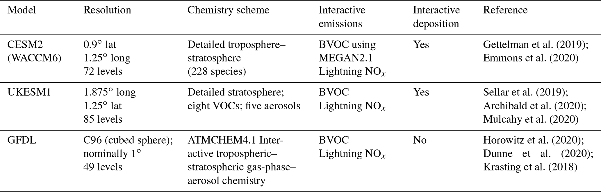
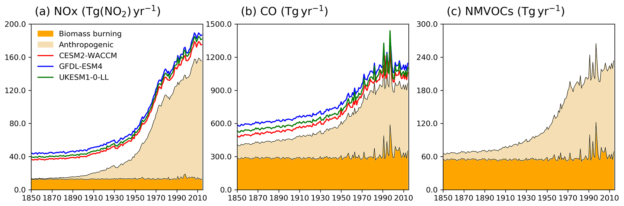
Figure 1Time evolution (1850–2014) of global total emissions for (a) NOx (Tg(NO2) yr−1), (b) CO (Tg(CO) yr−1), and (c) NMVOC (Tg(VOC) yr−1). Orange is for biomass burning, and beige is for anthropogenic emissions (Hoesly et al., 2018). The coloured lines in the NOx and CO panels (red for CESM2-WACCM, blue for GFDL-ESM4, and green for UKESM1-0-LL) are the total emissions for each model, including natural sources. For historical biogenic VOC emissions, see Griffiths et al. (2020, Fig. 1).
Two base historical transient experiments have been analysed: “historical” and “histSST” (Table 2). The historical runs included a fully coupled ocean and multiple ensemble members. The histSST simulations were single-member atmosphere-only runs, with monthly mean time-evolving sea surface temperatures (SSTs) and sea ice prescribed from one ensemble member of the historical simulations. Identical historical anthropogenic forcings were applied in all base runs by using prescribed long-lived greenhouse gas and halocarbon mole fractions (Meinshausen et al., 2017) as well as anthropogenic and biomass burning emissions of near-term climate forcers (NTCFs; i.e. aerosols, aerosol precursors, and ozone precursors) (van Marle et al., 2017; Hoesly et al., 2018). Emissions of NOx, CO, and NMVOC from 1850 to 2014 are shown in Fig. 1. Natural emissions of these species were either prescribed (e.g. soil NOx emissions, oceanic CO emissions) or internally calculated (e.g. biogenic isoprene, lightning NOx) by embedded process-based climate-dependent schemes that differ between models (e.g. Griffiths et al., 2020; Turnock et al., 2020). Methane mole fractions were prescribed at the surface based on observations and ice core data (Meinshausen et al., 2017); away from the surface, methane was simulated by the model. However, by prescribing surface mole fractions, methane throughout the model domain was effectively prescribed.
Table 2Number of ensemble members analysed from CMIP6 experiments in this study. All were transient 1850–2014 simulations with evolving land surfaces, trace species emissions, and greenhouse gas (GHG) mole fractions. Baseline historical runs had freely evolving oceans, whilst histSST runs were atmosphere-only with prescribed (observed) SSTs and sea ice. Sensitivity runs are based on histSST. The “-piNTCF” simulation held emissions of all NTCFs (aerosols, their precursors, and tropospheric ozone precursors) at PI levels. The “-1950HC” simulation held halocarbon mole fractions at 1950 levels (essentially PI levels). The “-piCH4” simulation held methane mole fractions at PI levels. The “-piO3” simulation held anthropogenic tropospheric ozone precursor emissions at PI levels.
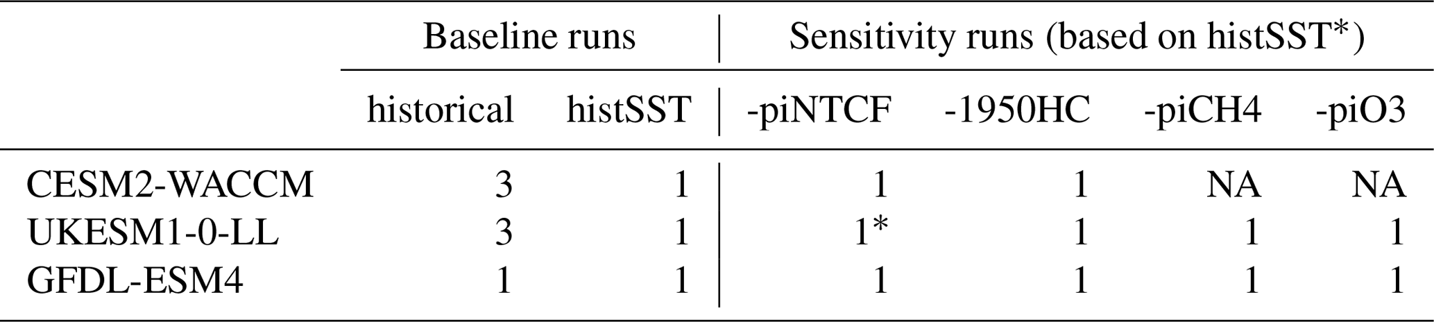
∗ UKESM1-0-LL sensitivity run for piNTCF is based on the historical (not histSST) run.
We also analysed several variants of the histSST base case with either methane mole fractions or emissions of NTCFs fixed at pre-industrial levels or halocarbon mole fractions fixed at 1950 levels. These variants allow us to estimate the roles of different drivers in changing OH (Table 2).
For some model variables we separated fields at the tropopause to provide a methane lifetime with respect to loss processes in the troposphere and stratosphere as separate values. We used World Meteorological Organization (WMO) defined tropopause pressures (the AerChemMIP variable ptp) from the models to diagnose this masking. The exact definition used is not critical, as most oxidation occurs well away from the tropopause in the tropical lower atmosphere (compare to tropospheric ozone, for which the tropopause definition is much more important; Griffiths et al., 2020).
Models diagnosed methane loss rates due to chemical destruction in each grid box – these are dominated by reaction with OH (Reaction R4) but also include other reactions, such as the reaction of methane with Cl in the stratosphere. We have used these loss rates to calculate grid box methane lifetimes. Whole-atmosphere chemical lifetimes were calculated by dividing the total methane burden by the total loss flux over the whole model domain, or just the troposphere or stratosphere, for tropospheric and stratospheric lifetimes.
We used the histSST-piNTCF simulations to diagnose the methane–OH feedback factor (Prather, 1996). These simulations held NTCF emissions at PI levels, but methane mole fractions evolved following their historical trajectory; from 1950 onwards, halocarbon mole fractions also increased. The methane–OH feedback is normally diagnosed from dedicated experiments that perturb only the methane mole fraction (Holmes, 2018), but such experiments are only available for PI conditions within AerChemMIP (e.g. Thornhill et al., 2020a). The methane–OH feedback factor, f, was calculated as follows:
where τ is the total methane lifetime, additionally including a soil sink; CH4 is taken to have a lifetime with respect to soil uptake of 160 years based on results for the 2000s from Spahni et al. (2011), Ito et al. (2012), Kirschke et al. (2013), and Tian et al. (2015), as summarized in Tian et al. (2016); the tropospheric Cl sink for methane is neglected here (Allan et al., 2007; Hossaini et al., 2016; Sherwen et al., 2016; Wang et al., 2019; Gromov et al., 2018; Strode et al., 2020); and [CH4] is the global mean methane mole fraction for a particular year (or range of years) of the histSST-piNTCF simulation. The reference year is 1850, the first year of the simulation. We took average values between 1930 and 1960 to give the most reliable estimate of f, as this is after a sufficiently large methane perturbation has built up but before halocarbons interfere with the results in these simulations (see Sect. 3.3).
We used each model's feedback factor to calculate equilibrium PD methane mole fractions ([CH4]eq) for each sensitivity run using the diagnosed total methane lifetimes from these experiments. The equilibrium methane mole fraction is the methane mole fraction that would have been reached if methane mole fractions had not been prescribed in these runs, but rather that methane emissions had been applied, allowing methane mole fractions to evolve freely (e.g. Fiore et al., 2009; Stevenson et al., 2013):
where [CH4]ref is the prescribed methane mole fraction in the run, and τref is the total methane lifetime in the histSST base experiment either for PD or, in the case of histSST-piCH4, for PI. We illustrate this with two examples: (i) in the histSST-piNTCF case, the equilibrium value is the PD methane mole fraction that would have been reached if all NTCF emissions been held at PI levels, whilst CH4 emissions had followed their historical evolution; and (ii) in the histSST-piCH4 case, the equilibrium value is the PD methane mole fraction that would have been reached if CH4 emissions had been held at PI levels, but all other emissions followed their historical evolution. This allows us to clarify modelled influences on CH4 from specific emissions.
2.2 Inferred OH from measurements
Tropospheric OH has a chemical lifetime of less than a second or so, reflecting its high reactivity and making direct measurement difficult and impractical for constraining global OH distributions (e.g. Stone et al., 2012). Instead, tropospheric mean OH and its variability have traditionally been inferred from measurements of trace gases with lifetimes longer than the timescale of tropospheric mixing and whose primary loss is via reaction with OH. If emissions are well-known, then observed changes in atmospheric abundance may be related, via inverse methods, to variations in OH. To date, the favoured proxy for estimating OH has been from measurements of methyl chloroform (1,1,1-trichloroethane; CH3CCl3; MCF), a synthetic industrial solvent that was banned in the late 1980s as a stratospheric-ozone-depleting substance (Lovelock, 1977; Singh, 1977; Spivakovsky et al., 1990, 2000; Montzka et al., 2000; Prinn et al., 2001). The inversions have typically spatially represented the global atmosphere as a few boxes.
The earliest MCF inversions predicted relatively large OH variability, reflecting high sensitivity to the uncertainty in residual MCF emissions (Bousquet et al., 2005; Prinn et al., 2005, 2001; Krol and Lelieveld, 2003; Krol et al., 2003). However, Montzka et al. (2011) demonstrated that by the late 1990s, residual emissions had declined sufficiently so as to be a minor source of uncertainty and that OH varied by at most a few percent in year-to-year variability. More recently, multi-box models have been used with Bayesian inverse methods to simultaneously optimize OH and MCF emissions to match MCF observations from NOAA and the Advanced Global Atmospheric Gases Experiment (AGAGE) networks, as well as multi-species inversions including methane and methane isotopologues as additional constraints (Rigby et al., 2017; Turner et al., 2017). Naus et al. (2019) further investigated the inversion methods used by Rigby et al. (2017) and Turner et al. (2017), confirming that the derivation of OH from MCF and CH4 is quite poorly constrained, and found that OH trends with a range of different magnitudes and signs were consistent with the available data.
Some inversion studies have used models with greater spatial resolution. McNorton et al. (2016) performed inverse modelling using a 3-D chemistry-transport model (CTM) constrained by MCF data and found that OH increases contributed significantly to the slowdown in the global CH4 growth rate between 1999 and 2006 and that the post-2007 increases in CH4 growth rate were poorly simulated if OH variations were ignored. McNorton et al. (2018) extended this work with further constraints from Greenhouse Gases Observing Satellite (GOSAT) CH4 and δ13CH4 and found that the post-2007 CH4 growth rate surge was most likely due to a combination of a decrease (−1.8 ± 0.4 %) in global OH and increases in CH4 emissions.

Figure 2(a) Time evolution of global annual mean tropospheric OH (1850–2014) expressed as a percentage anomaly relative to the 1998–2007 mean (and ensemble spreads where available) for GFDL-ESM4 (blue), UKESM1-0-LL (green), CESM2-WACCM (red), and the multi-model mean (black). (b) Observation-based inversions of global annual mean tropospheric OH for 1980–2015 from Montzka et al. (2011), Rigby et al. (2017), Turner et al. (2017), and Nicely et al. (2018), including ± 1 standard deviation uncertainties for the results from Rigby et al. (2017), with model results from (a) overlain.
These inversion studies generally find OH to have increased from the late 1980s until the mid-2000s when OH then began to decline (Fig. 2b). However, most inversion studies also found that solutions exist within the uncertainty of the system when OH was held constant and only emissions of the reactants were allowed to be optimized. In contrast, Nicely et al. (2018) empirically derived a historic global mean OH reconstruction by taking a baseline forward OH simulation from the National Aeronautics and Space Administration (NASA) Global Modeling Initiative (GMI) CTM driven by assimilated meteorology since 1980 and adjusting it based on box-model-derived relationships of OH responses to changes in observable parameters such as total ozone columns from satellites. The empirically derived OH reconstruction (also shown in Fig. 2b) was found to be relatively invariant when compared to other MCF inversions over the past few decades, which the study suggested reflected chemical buffering of the many competing factors that can influence OH.
Several studies have investigated the constraints imposed on OH by species other than MCF and CH4. Gaubert et al. (2017) assimilated time series of global-scale satellite CO measurements from the Measurements of Pollution In The Troposphere (MOPITT) project into a global model and found a decrease in the global CO burden of ∼ 20 % over the period 2002–2013. Associated with this decrease in CO was an 8 % shortening of the methane lifetime and a 7 % increase in OH. Nguyen et al. (2020) also found that decreasing global CO concentrations since the 2000s have important influences on CH4 flux inversion results because of the strong chemical coupling between CO, CH4, and OH. Assimilation of satellite CO, NOx, and O3 data (e.g. Miyazaki et al., 2015, 2017; Miyazaki and Bowman, 2017; Gaubert et al., 2017) demonstrates that OH is sensitive to all these species and that data assimilation improves simulation of the hemispheric ratio of OH (Patra et al., 2014).
Collectively, these earlier studies have shown that OH is influenced by CO, NO2, O3, and CH4. To date, studies have used subsets of the available observational data (i.e. one or more of MCF, CH4, δ13CH4, CO, NO2, and O3) to constrain OH but not yet all available relevant data. The OH trends derived from several of these studies, including the uncertainty estimates from Rigby et al. (2017), are summarized in Fig. 2b.
3.1 Pre-industrial to present-day base simulations
Figure 2a shows time series (1850–2014) of global annual mean tropospheric OH burden expressed as a percentage anomaly relative to the 1998–2007 mean value for the three models. This shows typical inter-annual variability in global OH of about ±2 %–3 %, a small decrease (about −3 %) in OH from 1850 up to 1910, then a similar magnitude increase up to the 1980s. From the 1980s to 2014, the models show a strong increase in OH of about 9 %. All three models show comparable behaviour. We find very similar results between the fully coupled (historical) and the atmosphere-only (histSST) experiments (not shown). This confirms that it is valid to directly compare and analyse together the results from these two experimental set-ups.
Figure 2b shows several estimates of global tropospheric OH trends over the period 1980–2014 inferred from observations (as described in Sect. 2.2), including an uncertainty range from Rigby et al. (2017). The inferred trends from different inversion methods show quite a wide range but are generally upwards from 1980 to 2005, in broad agreement with the AerChemMIP models. However, from 2005 onwards, the inversions generally indicate downwards trends, whereas the models suggest a continued slight upwards trend. The 1980–2015 model global OH trends are almost always within the ±1 standard deviation uncertainty range from Rigby et al. (2017), although they are close to the lower end of the range in 1980 and just beyond its upper end in 2015.
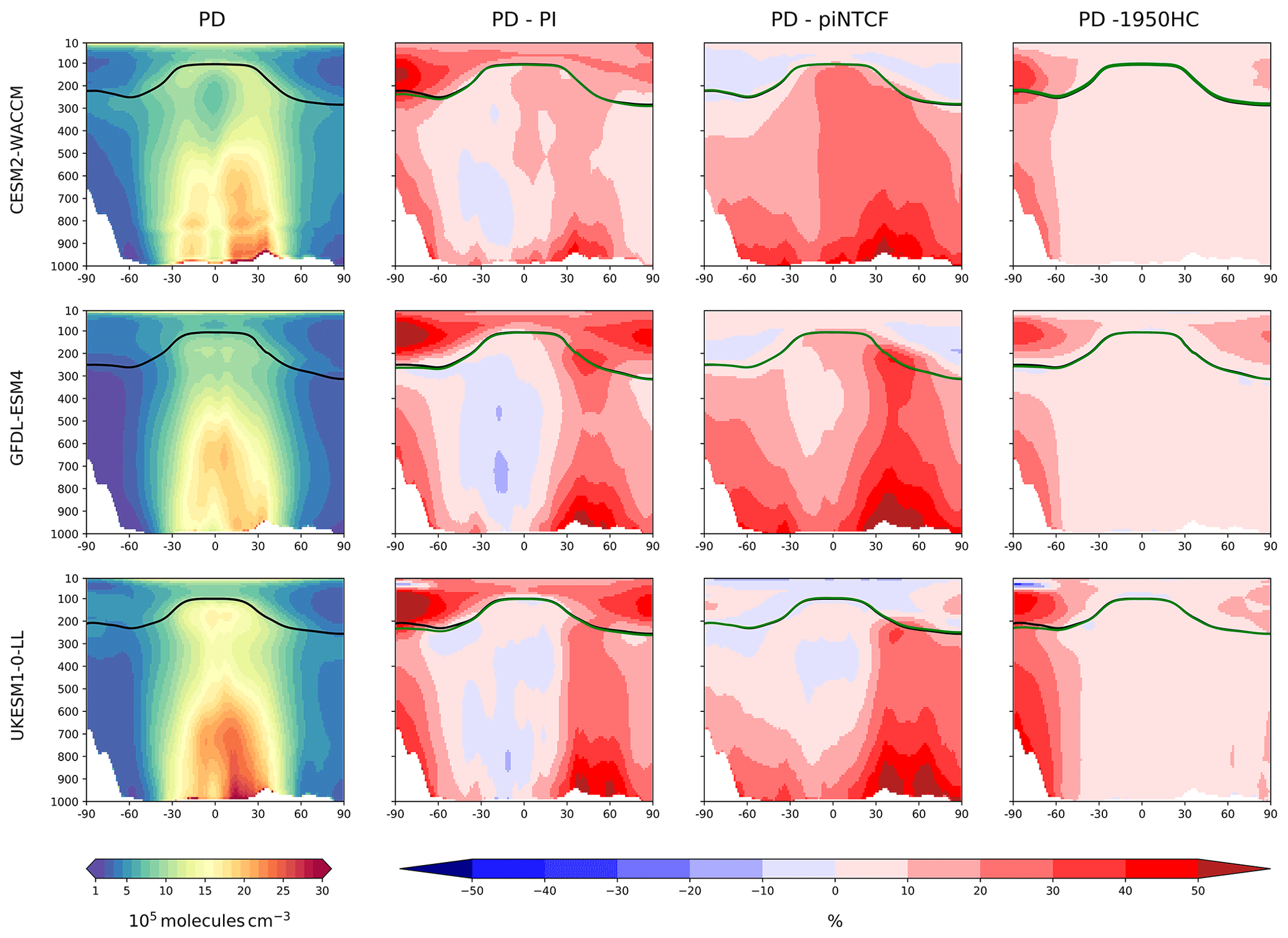
Figure 3First column: zonal mean (latitude–pressure, hPa) cross sections for OH concentration (105 molec. cm−3) averaged over the period 2005–2014 (PD) for the histSST simulations. Rows show results for CESM2-WACCM, GFDL-ESM4, and UKESM1-0-LL. Solid lines indicate the tropopause (PD in black; other in green). Other panels show differences (%) between experiments. Second column: histSST PD minus PI (1850–1859 mean). Third column: histSST minus histSST-piNTCF for PD. Fourth column: histSST minus histSST-1950HC for PD.
Figure 3 shows present-day (PD; 2005–2014 decadal mean) zonal mean OH concentrations for the three models. The vertical coordinate is pressure, and the zonal mean WMO tropopause is indicated. All models show high OH values between 30∘ S and 30∘ N in the lower to middle troposphere, with larger values in the Northern Hemisphere (NH).
Figure 3 also shows changes in OH from pre-industrial (PI; 1850–1859 decadal mean) to PD expressed as the percentage change relative to PD. This reveals local increases of over 50 % in zonal mean tropospheric OH, in particular over polluted NH mid-latitudes, but also a local decrease of over 10 % in the Southern Hemisphere (SH) middle to upper troposphere at around 20∘ S. The PD–PI figures also show both the PD and PI tropopauses and indicate insignificant changes in tropopause height over the historical era.
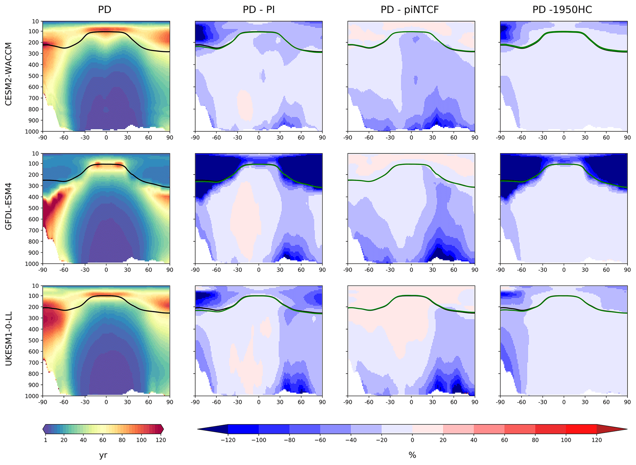
Figure 4 shows the zonal mean distribution of local methane lifetime, which ranges from about 2.5 years in the tropical lower troposphere to > 20 years in colder, drier high latitudes and in the vicinity of the tropopause. Short lifetimes also occur higher in the stratosphere but do not significantly contribute to the whole-atmosphere chemical lifetime due to the low air densities at high altitudes. The multi-model mean whole-atmosphere PD chemical lifetime in histSST is 8.4 ± 0.3 years, lower than the mean PI lifetime of 9.5 ± 0.5 years (lifetimes for individual models are given in Table 3; the ranges are the standard deviations across the models). These values compare to a whole-atmosphere methane lifetime for 2010 (mean ± 1 standard deviation) of 9.1 ± 0.9 years (Prather et al., 2012), as used by the Intergovernmental Panel on Climate Change (IPCC; Myhre et al., 2013). Lifetimes have fallen since the PI, mainly reflecting increases in OH.
Table 3Whole-atmosphere methane chemical (not including soil sink) lifetimes (years). PI refers to the 1850–1859 mean; PD refers to the 2005–2014 mean. Uncertainties are ±1 standard deviation based on the range of annual values.
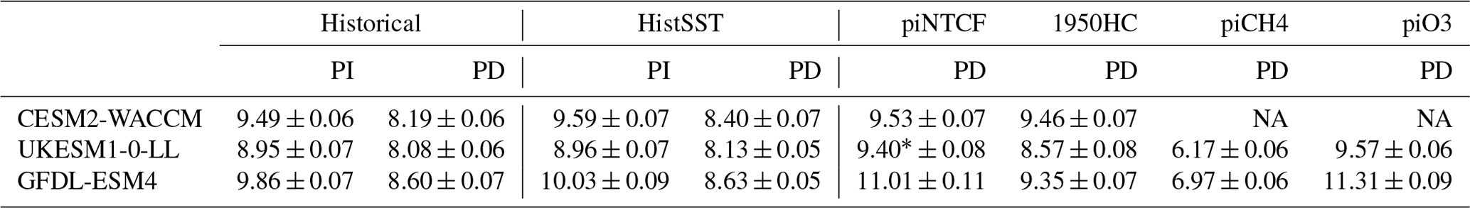
∗ UKESM1-0-LL methane lifetime for piNTCF is based on the historical (not histSST) run.
3.2 Historical sensitivity simulations
The drivers of these changes in OH and methane lifetime were explored further using results from sensitivity experiments based on the histSST simulations. These kept anthropogenic emissions or mole fractions of particular species, or groups of species, at their PI or 1950 levels (Table 2). Figure 3 shows how zonal mean OH in the models responded to fixing NTCF emissions at PI levels and halocarbon mole fractions at 1950 levels. The panels in Fig. 3 shows percentage changes in OH relative to the PD histSST base case. Figure 4 shows percentage changes in methane lifetime.
We define the annual tropospheric OH burden anomaly in the base histSST simulations at time t (ΔOHBase(t)) as the percentage change in OH since PI (1850–1859):
or, for clarity, dropping the (t) and substituting OHPI for OHhistSST(PI):
We then use each sensitivity run to isolate the contributions to this overall OH anomaly from changes in CH4 mole fraction, NTCF emissions, halocarbon mole fraction, and O3 precursor emissions since 1850:
Since the ΔOHNTCF and ΔOH anomalies only differ in that the former includes the effects of aerosols, then assuming that the impacts of aerosols and O3 precursors on OH do not interact with each other, we can also isolate the contribution from changes in aerosols to the overall OH anomaly:
In addition, we can calculate a “residual” contribution, i.e. the component of the overall OH anomaly that is left after linearly adding all the other components:
This residual component represents the contribution of climate change to the OH anomaly, along with any contributions from non-linear interactions between components. Non-linearities may arise, for example, because the response of OH to changes in CH4 is likely to differ depending on whether NTCFs, such as NOx, are at PI or PD levels. Such interactions are not isolated by our methodology, and it is unclear whether the climate change signal or the effects of non-linearities dominate this residual term.

Figure 5The histSST (base, in black) tropospheric OH anomaly (percent change relative to PI) for each year (see Eq. 3) for the three models: (a) CESM2-WACCM, (b) GFDL-ESM4, and (c) UKESM1-0-LL. The coloured lines represent the contributions to this OH anomaly due to changes since 1850 in CH4 mole fraction, NTCF emissions, halocarbon mole fraction, O3 precursor emissions, and aerosols (see Eqs. 4–8; only NTCF and HC experiments from CESM2-WACCM). The residual curve (see Eq. 9) is the extra contribution required after linearly adding the curves for CH4, NTCF, and HC that is needed to reproduce the base anomaly.
Figure 5 shows time series of how the base OH anomaly (Eq. 3) evolves, together with each of the components (Eqs. 4–9) that contribute to the base anomaly. Figure 6 compares the magnitudes of these various drivers of OH changes over two time periods: 1850–1980 and 1850–2010. Figure 7 shows the evolution of whole-atmosphere methane lifetime for the base histSST runs and each sensitivity run. Figure 7 also separates the methane lifetime into its tropospheric and stratospheric components.

Figure 6Summary of drivers of OH changes (%) relative to 1850 for the three models and their multi-model mean over (a) 1850–1980 and (b) 1850–2010. We have used decadal means: 1850 refers to 1850–1859, 1980 is 1975–1984, and 2010 is 2005–2014. The shaded areas show the split of the NTCF signal (green) into ozone precursors (blue) and aerosols (brown) when models have performed both the histSST-piNTCF and histSST-piO3 experiments. The residual values (pale blue) are the differences between the total change (black, from the histSST simulations) and the sum of the changes from CH4 (red), NTCF, and halocarbons (purple). We interpret the residual terms as being due to climate change, in addition to any non-linear interactions between forcings.
Figures 5 and 6 show that the evolution of OH has been mainly controlled by the balance between the growth of methane, which has acted to reduce OH by over 20 %, and the changes in NTCF emissions (and in UKESM1-0-LL, the residual term), which have tended to increase OH. Because these opposing drivers have similar magnitudes, small mismatches between them are key, and the other minor drivers can also be important contributors to the overall trend in OH.
The impact of increases in NTCF emissions since 1850 up to PD was to generally increase tropospheric OH by 10 %–50 % in the zonal mean (Fig. 3) and 13 %–22 % across the whole troposphere (Figs. 5 and 6); this mainly reflects the dominant role of NOx increases, whose impact overwhelms the impacts of increasing CO (up to ∼ 1990) and NMVOC emissions, which will have tended to reduce OH. Since about 1990, global CO emissions have been reduced (Fig. 1), also contributing to the increase in OH. The overall impact of changed emissions of NTCFs has been to reduce the methane lifetime (Figs. 4 and 7, Table 3). This is mainly driven by increases in NOx emissions. The structure seen in the zonal mean PD–PI change in OH (Fig. 3, column 2) can be largely explained by the change in NTCF emissions (Fig. 3, column 3), with the effects of methane mole fraction increases superimposed. Note that increasing methane also increases CO, and both these reduce OH. We are unable to isolate the effects of CO in our experiments.
Emissions of halocarbons since 1950 have led to polar stratospheric ozone depletion, mainly in the SH. This has increased stratospheric OH levels but also increased tropospheric OH due to increased penetration of ultraviolet (UV) radiation and consequently higher photolysis rates (Fig. 3). The overall impact on tropospheric OH and methane lifetime is comparatively small (Figs. 4–7, Table 3), but the impact on methane lifetime in the stratosphere has been dramatic, reducing it from ∼ 170 to ∼ 140 years (CESM2-WACCM), from ∼ 140 to ∼ 80 years (GFDL-ESM4), and from ∼ 190 to 145 years (UKESM1-0-LL) (Fig. 7). These changes are mainly driven by changes in stratospheric Cl. These values can be compared to an assumed constant value for the lifetime of methane with respect to stratospheric chemical destruction of 120 (±20 %) years in the IPCC Fifth Assessment Report (Prather et al., 2012).
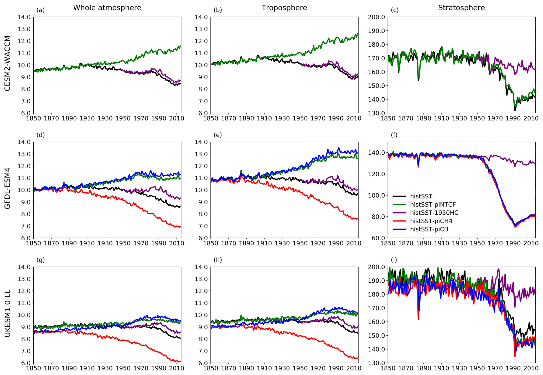
Figure 7Time evolution (1850–2014) of CH4 lifetime (years) for (a–c) CESM2-WACCM, (d–f) GFDL-ESM4, and (g–i) UKESM-0-LL averaged over the whole atmosphere (a, d, g), the troposphere (b, e, h), and the stratosphere (c, f, i). Colours refer to different model experiments, as indicated in (f). For UKESM-0-LL, we used historical-piNTCF as histSST-piNTCF was not available.
The effects of increased emissions of aerosols and aerosol precursors can be diagnosed by differencing the piO3 and piNTCF simulations (Eq. 8). Aerosols have slightly reduced OH (Figs. 5 and 6) and lengthened the methane lifetime (Fig. 7), but the effect is small in magnitude compared to most other effects.
For the two models able to diagnose the residual term, they both suggest a positive impact on OH although by variable amounts (6 %–13 %), with a larger residual term in UKESM1-0-LL. We suggest this term may reflect increases in humidity associated with climate change and an increase in the primary OH production flux (Reaction R2). However, exactly what the residual terms represent remains uncertain.
3.3 Contribution of OH drivers to PI–PD changes in methane
Figure 7 shows values for the methane–OH feedback factor (from a modified version Eq. (1) using values for individual years rather than 1930–1960) calculated for every year in the histSST-piNTCF simulations. In the first few decades, the methane changes are small and the variability of the methane lifetime yields large fluctuations in f. Beyond about 1960, changes in halocarbon mole fractions mean that the values of f are unreliable. We therefore use the average value over the time period 1930–1960 as our best estimate of the feedback factor. This yields a value of 1.25 for CESM2-WACCM and 1.23 for GFDL-ESM4. Thornhill et al. (2020a) find values of f from the piClim simulations of 1.30 for GFDL-ESM4 and 1.32 for UKESM1-0-LL. The values derived using Eq. (1) are probably slightly smaller because the histSST-piNTCF runs also include increases in temperature and humidity. These values are similar to the range of values found in previous studies: 1.23–1.35 (Stevenson et al., 2013; six models), 1.19–1.28 (Voulgarakis et al., 2013; two models, year 2000 conditions), and 1.33–1.45 (Prather et al., 2001; seven models). Using the values of f for 1930–1960 (Fig. 7) for CESM2-WACCM and GFDL-ESM4, the value of 1.32 for UKESM1-0-LL (Thornhill et al., 2020a), and the lifetimes presented in Table 3, we calculate equilibrium PD methane mole fractions for all sensitivity experiments (Table 4).
Table 4Equilibrium PD global mean methane mole fractions (ppbv) inferred from PD methane lifetimes from the sensitivity experiments. Also shown are percentage changes compared to the observed PD value (1794 ppbv) or, for the piCH4 case, the observed PI value (808 ppbv).
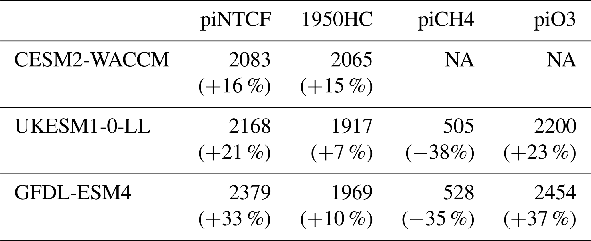
Observed PI and PD methane levels are 808 and 1794 ppb, respectively. Holding NTCFs at PI levels increases PD methane by 16 %–33 %. This is more intuitively interpreted in terms of the impact of the increased emissions of NTCFs: they have tended to reduce PD methane by this amount. Similarly, the impact of halocarbon emissions has been to reduce PD methane by 7 %–15%.
Taking the average of results from the GFDL-ESM4 and UKESM1-0-LL models (that have values for all categories), holding methane emissions at PI levels would have led to PD methane levels of 516 ppbv, which is 36 % (292 ppbv) lower than PI mole fractions. Hence, the net impact of increasing methane emissions has been to increase methane mole fractions from 516 to 1794 ppbv, an increase of 1278 ppbv . This increase is 30 % larger than the simple observed PI to PD increase in methane (986 ppbv, ). The impact of NTCF emissions was to reduce PD methane by 480 ppbv (), whilst increases in halocarbon emissions reduced PD methane by 149 ppbv (). These diagnosed contributions do not linearly add up to give the observed total; there is a residual term, as also found when attributing the OH changes to drivers. Following a similar format to Eq. (9), we can diagnose this residual term:
We tentatively attributed the OH residual term to climate change impacts, as the residual OH increase could physically be linked to water vapour increases. However, the residual change in equilibrium methane is positive, whilst it would be expected to be negative in order to match the positive residual OH term. The other attributions for OH and equilibrium methane are more well-behaved and consistent. This suggests that non-linear interactions between drivers are important and differ in strength between our attribution methodologies for OH and methane. This means that perfect quantitative attribution cannot be achieved, and attribution of the residual term to climate change effects is rather uncertain. Nevertheless, the magnitudes of these attribution terms are useful qualitative indicators of the relative importance of different drivers of changes in OH and methane lifetime.
Modelled OH trends presented in this study are from state-of-the-art Earth system models driven by CMIP6 historical forcings, including observed trends in CH4 and halocarbon mole fractions. The latter drive stratospheric ozone depletion in the models, which strongly influences tropospheric UV levels and hence photolysis rates. Apart from CH4, all other reactive species that control OH (e.g. CO, O3, NO2, and H2O) freely evolve in the simulations in response to prescribed CMIP6 emissions and simulated climate. These model simulations of OH are very important for understanding past trends and projecting future trends in CH4.
The base model simulations all show similar historical trends in global OH, with relative stability from 1850 up to 1980, followed by strong (9 %) increases up to the present day (Fig. 2). The earlier stability is in good agreement with previous studies (e.g. Naik et al., 2013). The increase from 1980 to 2005 is broadly consistent with several studies that use MCF and other species to reconstruct OH trends from observations; however, since 2005 most of these reconstructions indicate a decrease in OH, whereas our models indicate a continued increase (Fig. 2b). However, these reconstructions show a wide range of trends, and our modelled trends fall just about within the uncertainty range estimated by Rigby et al. (2017). The magnitudes of the model's recent increases are similar to results from Gaubert et al. (2017), who assimilated satellite-derived trends in CO since 2002 into an Earth system model. Several OH inversions have used multiple observational datasets (Miyazaki et al., 2015; McNorton et al., 2018), and as the time series of observations, particularly satellite data, lengthens, uncertainties on real-world OH trends will hopefully be reduced, providing stronger constraints for models.
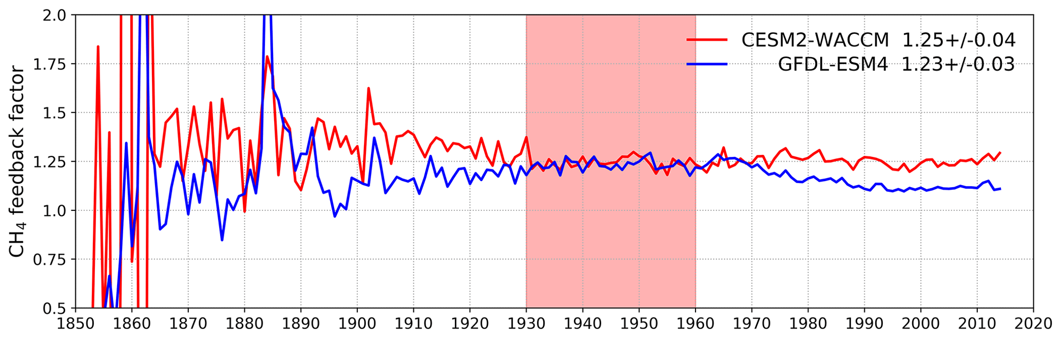
Figure 8Calculated values for the methane–OH feedback factor (f) from the histSST-piNTCF experiments for CESM2-WACCM and GFDL-ESM4. Mean and standard deviation values for 1930–1960 (shaded time period) are shown.
We attempted to quantify the component drivers of the changes in OH using a series of idealized model sensitivity experiments. These experiments exhibit relatively consistent OH responses across the models (Figs. 5 and 6) and show that the evolution of methane and ozone precursor emissions have strongly influenced OH trends. Halocarbon and aerosol-related emissions have had relatively small impacts. We also diagnose a residual component that represents the impact of climate change and non-linear interactions between drivers. Other studies have indicated that climate variations and change influence OH (e.g. Naik et al., 2013; Murray et al., 2014; Turner et al., 2018). The modelled increase in OH since 1980 is because the influence of NTCF emissions, together with this residual term, outweighs the effects of increasing CH4 (Fig. 6). These experiments did not separate the effects of different ozone precursors, but these have been explored in previous studies (Stevenson et al., 2013; Holmes et al., 2013), wherein increases in anthropogenic NOx emissions have been found to be the main NTCF driver of OH increases. Recent reductions in anthropogenic CO emissions (Fig. 1) are clearly also important (Gaubert et al., 2017), but our experiments are unable to separate the relative impacts of these two species.
The trends in OH are associated with trends in methane lifetime (Fig. 7), and we have used these to estimate the influence of individual drivers on the methane mole fraction by calculating equilibrium methane levels from the changes in lifetime (Table 4). Drivers that increase OH lead to reductions in methane lifetime and equilibrium methane. The residual component for OH is positive and may mainly physically represent the rise of water vapour associated with climate warming. This finding is broadly consistent with results presented by Thornhill et al. (2020b) of the negative impacts on methane lifetime found in 4×CO2 experiments (see their Table 15). However, the residual component we diagnosed from changes in equilibrium methane is also positive, which suggests that non-linear interactions show different impacts in our two methodologies that diagnose residual effects and that the residual term may not be a good indicator of climate change effects alone. These results indicate that methodologies to isolate drivers of OH and methane changes need careful interpretation, as non-linearities (i.e. couplings between drivers) appear to be important.
Although halocarbon emissions have had quite small effects on the whole-atmosphere methane lifetime, they have had dramatic impacts on methane's stratospheric chemistry, and its lifetime may have been reduced by up to about 40 % between 1960 and 1990 (Fig. 7). Previous studies have generally assumed a fixed stratospheric lifetime for methane (e.g. Prather et al., 2012).
All these factors need to be included in holistic assessments of OH and methane change. The CMIP6/AerChemMIP model simulations contain many useful diagnostics that will allow us to better understand the drivers of atmospheric OH and methane trends. This study represents a very preliminary initial analysis of this rich multi-model, multi-experiment dataset.
This work uses simulations from multiple models participating in the AerChemMIP project as part of the Coupled Model Intercomparison Project (Phase 6; https://www.wcrp-climate.org/wgcm-cmip, World Climate Research Program, 2020); model-specific information can be found through references listed in Table 1. Model outputs are available on the Earth System Grid Federation (ESGF) website (https://esgf-data.dkrz.de/search/cmip6-dkrz/, Earth System Grid Federation, 2020). The model outputs were preprocessed using the NetCDF Operator (NCO) and Climate Data Operator (CDO). The analysis was carried out using Bash and Python programming languages.
A large team of modellers generated the data used in this study: VN, LWH, and LTS produced the GFDL model data; FMO'C, GZ, PG, and SS produced the UKESM data; ST and LE produced the CESM data. AZ synthesized and analysed the data and produced the figures. DSS wrote the paper, incorporating comments from all authors.
The authors declare that they have no conflict of interest.
This article is part of the special issue “The Aerosol Chemistry Model Intercomparison Project (AerChemMIP)”. It is not associated with a conference.
VN, LWH, and LTS thank the GFDL model development team and the leadership of NOAA/GFDL for their efforts and support in developing ESM4 as well as the GFDL modelling systems group and data portal team for technical support to make data available at the ESGF. ST, LE, and the CESM project are supported primarily by the National Science Foundation (NSF). Computing and data storage resources, including the Cheyenne supercomputer (https://doi.org/10.5065/D6RX99HX, last access: 3 November 2020), were provided by the Computational and Information Systems Laboratory (CISL) at NCAR.
David S. Stevenson received support from the Natural Environment Research Council under grants NE/N003411/1 and NE/S009019/1 as well as the ARCHER UK National Supercomputing Service (http://www.archer.ac.uk, last access: 3 November 2020). Alcide Zhao received support from a Joint Scholarship from the China Scholarships Council–University of Edinburgh and the UK–China Research and Innovation Partnership Fund through the Met Office Climate Science for Service Partnership (CSSP) China as part of the Newton Fund (grant no. H5438500). Guang Zeng was supported by the NZ government's Strategic Science Investment Fund (SSIF). William J. Collins received funding from the European Union's Horizon 2020 research and innovation programme under grant agreement no. 641816 (Co-ordinated Research in Earth Systems and Climate: Experiments, Knowledge, Dissemination and Outreach – CRESCENDO – https://www.crescendoproject.eu/, last access: 3 November 2020). This material is based upon work supported by the National Center for Atmospheric Research, which is a major facility sponsored by the NSF under cooperative agreement no. 1852977. Sungbo Shim was supported by the Korea Meteorological Administration Research and Development Program “Development and Assessment of IPCC AR6 Climate Change Scenario”, grant agreement number KMA2018-00321. Fiona M. O'Connor was supported by the Department for Business, Energy and Industrial Strategy/Department for Environment, Food and Rural Affairs Met Office Hadley Centre Climate Programme (grant no. GA01101) and the Horizon 2020 Framework Programme (CRESCENDO, grant no. 779366).
This paper was edited by Jennifer G. Murphy and reviewed by two anonymous referees.
Allan, W., Struthers, H., and Lowe, D.: Methane carbon isotope effects caused by atomic chlorine in the marine boundary layer: Global model results compared with Southern Hemisphere measurements, J. Geophys. Res.-Atmos., 112, D04306, https://doi.org/10.1029/2006JD007369, 2007.
Archibald, A. T., O'Connor, F. M., Abraham, N. L., Archer-Nicholls, S., Chipperfield, M. P., Dalvi, M., Folberth, G. A., Dennison, F., Dhomse, S. S., Griffiths, P. T., Hardacre, C., Hewitt, A. J., Hill, R. S., Johnson, C. E., Keeble, J., Köhler, M. O., Morgenstern, O., Mulcahy, J. P., Ordóñez, C., Pope, R. J., Rumbold, S. T., Russo, M. R., Savage, N. H., Sellar, A., Stringer, M., Turnock, S. T., Wild, O., and Zeng, G.: Description and evaluation of the UKCA stratosphere-troposphere chemistry scheme (StratTrop vn 1.0) implemented in UKESM1, Geosci. Model Dev., 13, 1223–1266, https://doi.org/10.5194/gmd-13-1223-2020, 2020.
Bousquet, P., Hauglustaine, D. A., Peylin, P., Carouge, C., and Ciais, P.: Two decades of OH variability as inferred by an inversion of atmospheric transport and chemistry of methyl chloroform, Atmos. Chem. Phys., 5, 2635–2656, https://doi.org/10.5194/acp-5-2635-2005, 2005.
Collins, W. J., Lamarque, J.-F., Schulz, M., Boucher, O., Eyring, V., Hegglin, M. I., Maycock, A., Myhre, G., Prather, M., Shindell, D., and Smith, S. J.: AerChemMIP: quantifying the effects of chemistry and aerosols in CMIP6, Geosci. Model Dev., 10, 585–607, https://doi.org/10.5194/gmd-10-585-2017, 2017.
Derwent R. G.: The influence of human activities on the distribution of hydroxyl radicals in the troposphere, Philos. T. Roy. Soc. A, 354, 501–531, https://doi.org/10.1098/rsta.1996.0018, 1996.
Dunne, J. P., Horowitz, L. W., Adcroft, A. J., et al.: The GFDL Earth System Model version 4.1 (GFDL-ESM 4.1): Overall coupled model description and simulation characteristics, J. Adv. Model. Earth Syst., 12, e2019MS002015, https://doi.org/10.1029/2019MS002015, 2020.
Emmons, L. K., Schwantes, R. H., Orlando, J. J., Tyndall, G., Kinnison, D., Lamarque, J.-F., Marsh, D., Mills, M., Tilmes, S., Bardeen, C., Buchholz, R. R., Conley, A., Gettelman, A., Garcia, R., Simpson, I., Blake, D. R., Meinardi, S., and Pétron, G.: The Chemistry Mechanism in the Community Earth System Model version 2 (CESM2), J. Adv. Model Earth Syst., 12, https://doi.org/10.1029/2019MS001882, 2020.
Earth System Grid Federation: WCRP CMIP6 data portal, available at: https://esgf-data.dkrz.de/search/cmip6-dkrz/, last access: 3 November 2020.
Eyring, V., Bony, S., Meehl, G. A., Senior, C. A., Stevens, B., Stouffer, R. J., and Taylor, K. E.: Overview of the Coupled Model Intercomparison Project Phase 6 (CMIP6) experimental design and organization, Geosci. Model Dev., 9, 1937–1958, https://doi.org/10.5194/gmd-9-1937-2016, 2016.
Fiore, A. M., Dentener, F. J., Wild, O., Cuvelier, C., Schultz, M. G., Hess, P., Textor, C., Schulz, M., Doherty, R. M., Horowitz, L. W., MacKenzie, I. A., Sanderson, M. G., Shindell, D. T., Stevenson, D. S., Szopa, S., Van Dingenen, R., Zeng, G., Atherton, C., Bergmann, D., Bey, I., Carmichael, G., Collins, W. J., Duncan, B. N., Faluvegi, G., Folberth, G., Gauss, M., Gong, S., Hauglustaine, D., Holloway, T., Isaksen, I. S. A., Jacob, D. J., Jonson, J. E., Kaminski, J. W., Keating, T. J., Lupu, A., Marmer, E., Montanaro, V., Park, R. J., Pitari, G., Pringle, K. J., Pyle, J. A., Schroeder, S., Vivanco, M. G., Wind, P., Wojcik, G., Wu, S., and Zuber, A.: Multi-model Estimates of Intercontinental Source Receptor Relationships for Ozone Pollution, J. Geophys. Res., 114, D04301, https://doi.org/10.1029/2008JD010816, 2009.
Gaubert, B., Worden, H. M., Arellano, A. F. J., Emmons, L. K., Tilmes, S., Barré, J., Martinez Alonso, S., Vitt, F., Anderson, J. L., Alkemade, F., Houweling, S., and Edwards, D. P.: Chemical feedback from decreasing carbon monoxide emissions, Geophys. Res. Lett., 44, https://doi.org/10.1002/2017GL074987, 2017.
Gettelman, A., Mills, M. J., Kinnison, D. E., Garcia, R. R., Smith, A. K., Marsh, D. R., Tilmes, S., Vitt, F., Bardeen, C. G., McInerney, J., Liu, H.-L., Solomon, S. C., Polvani, L. M., Emmons, L. K., Lamarque, J.-F., Richter, J. H., Glanville, A. S., Bacmeister, J. T., Phillips, A. S., Neale, R. B., Simpson, I. R., DuVivier, A. K., Hodzic, A., and Randel, W. J.: The Whole Atmosphere Community Climate Model Version 6 (WACCM6), J. Geophys. Res.-Atmos., 124, 12380–12403, https://doi.org/10.1029/2019JD030943, 2019.
Griffiths, P. T., Murray, L. T., Zeng, G., Archibald, A. T., Emmons, L. K., Galbally, I., Hassler, B., Horowitz, L. W., Keeble, J., Liu, J., Moeini, O., Naik, V., O'Connor, F. M., Shin, Y. M., Tarasick, D., Tilmes, S., Turnock, S. T., Wild, O., Young, P. J., and Zanis, P.: Tropospheric ozone in CMIP6 Simulations, Atmos. Chem. Phys. Discuss., https://doi.org/10.5194/acp-2019-1216, in review, 2020.
Gromov, S., Brenninkmeijer, C. A. M., and Jöckel, P.: A very limited role of tropospheric chlorine as a sink of the greenhouse gas methane, Atmos. Chem. Phys., 18, 9831–9843, https://doi.org/10.5194/acp-18-9831-2018, 2018.
Hoesly, R. M., Smith, S. J., Feng, L., Klimont, Z., Janssens-Maenhout, G., Pitkanen, T., Seibert, J. J., Vu, L., Andres, R. J., Bolt, R. M., Bond, T. C., Dawidowski, L., Kholod, N., Kurokawa, J.-I., Li, M., Liu, L., Lu, Z., Moura, M. C. P., O'Rourke, P. R., and Zhang, Q.: Historical (1750–2014) anthropogenic emissions of reactive gases and aerosols from the Community Emissions Data System (CEDS), Geosci. Model Dev., 11, 369–408, https://doi.org/10.5194/gmd-11-369-2018, 2018.
Holmes, C. D.: Methane feedback on atmospheric chemistry: Methods, models, and mechanisms, J. Adv. Model. Earth Sy., 10, 1087–1099, https://doi.org/10.1002/2017MS001196, 2018.
Holmes, C. D., Prather, M. J., Søvde, O. A., and Myhre, G.: Future methane, hydroxyl, and their uncertainties: key climate and emission parameters for future predictions, Atmos. Chem. Phys., 13, 285–302, https://doi.org/10.5194/acp-13-285-2013, 2013.
Horowitz, L. W., Naik, V., Paulot, F., et al.: The GFDL Global Atmospheric Chemistry-Climate Model AM4.1: Model Description and Simulation Characteristics, J. Adv. Model. Earth Sy., 12, e2019MS002032, https://doi.org/10.1029/2019MS002032, 2020.
Hossaini, R., Chipperfield, M. P., Saiz-Lopez, A., Fernandez, R., Monks, S., Feng, W., Brauer, P., and von Glasow, R.: A global model of tropospheric chlorine chemistry: Organic versus inorganic sources and impact on methane oxidation, J. Geophys. Res.-Atmos., 121, 14271–14297, https://doi.org/10.1002/2016JD025756, 2016.
IPCC, 2013: Annex II: Climate System Scenario Tables, edited by: Prather, M., Flato, G., Friedlingstein, P., Jones, C., Lamarque, J.-F., Liao, H., and Rasch, P., in: Climate Change 2013: The Physical Science Basis. Contribution of Working Group I to the Fifth Assessment Report of the Intergovernmental Panel on Climate Change, edited by: Stocker, T. F., Qin, D., Plattner, G.-K., Tignor, M., Allen, S. K., Boschung, J., Nauels, A., Xia, Y., Bex, V., and Midgley, P. M., Cambridge University Press, Cambridge, United Kingdom and New York, NY, USA, 1395–1445, 2013.
Isaksen, I. S. A., Granier, C., Myhre, G., Berntsen, T. K., Dalsøren, S. B., Gauss, M., Klimont, Z., Benestad, R., Bousquet, P., Collins, W., Cox, T., Eyring, V., Fowler, D., Fuzzi, S., Jöckel, P., Laj, P., Lohmann, U., Maione, M., Monks, P., Prevot, A. S. H., Raes, F., Richter, A., Rognerud, B., Schulz, M., Shindell, D., Stevenson, D. S., Storelvmo, T., Wang, W.-C., van Weele, M., Wild, M., and Wuebbles, D.: Atmospheric composition change: Climate-Chemistry interactions, Atmos. Environ., 43, 5138–5192, https://doi.org/10.1016/j.atmosenv.2009.08.003, 2009.
Ito, A. and Inatomi, M.: Use of a process-based model for assessing the methane budgets of global terrestrial ecosystems and evaluation of uncertainty, Biogeosciences, 9, 759–773, https://doi.org/10.5194/bg-9-759-2012, 2012.
Kirschke, S., Bousquet, P., Ciais, P., Saunois, M., Canadell, J. G., Dlugokencky, E. J., Bergamaschi, P., Bergmann, D., Blake, D. R., Bruhwiler, L., Cameron-Smith, P., Castaldi, S., Chevallier, F., Feng, L., Fraser, A., Heimann, M., Hodson, E. L., Houweling, S., Josse, B., Fraser, P. J., Krummel, P. B., Lamarque, J.-F., Langenfelds, R. L., Le Quere, C., Naik, V., O'Doherty, S., Palmer, P. I., Pison, I., Plummer, D., Poulter, B., Prinn, R. G., Rigby, M., Ringeval, B., Santini, M., Schmidt, M., Shindell, D. T., Simpson, I. J., Spahni, R., Steele, L. P., Strode, S. A., Sudo, K., Szopa, S., van der Werf, G. R., Voulgarakis, A., van Weele, M., Weiss, R. F., Williams, J. E., and Zeng, G.: Three decades of global methane sources and sinks, Nat. Geosci., 6, 813–823, https://doi.org/10.1038/NGEO1955, 2013.
Krasting, J. P., John, J. G., Blanton, C., et al.: NOAA-GFDL GFDL-ESM4 model output prepared for CMIP6 CMIP. Version 20180701, Earth System Grid Federation, https://doi.org/10.22033/ESGF/CMIP6.1407, 2018.
Krol, M., and Lelieveld, J.: Can the variability in tropospheric OH be deduced from measurements of 1,1,1-trichloroethane (methyl chloroform)?, J. Geophys. Res., 108, 4125, https://doi.org/10.1029/2002JD002423, 2003.
Krol, M., Lelieveld, J., Oram, D., Sturrock, G., Penkett, S., Brenninkmeijer, C., Gros, V., Williams, J., and Scheeren, H.: Continuing emissions of methyl chloroform from Europe, Nature, 421, 131–135, https://doi.org/10.1038/nature01311, 2003.
Lawrence, M. G., Jöckel, P., and von Kuhlmann, R.: What does the global mean OH concentration tell us?, Atmos. Chem. Phys., 1, 37–49, https://doi.org/10.5194/acp-1-37-2001, 2001.
Lelieveld, J., Gromov, S., Pozzer, A., and Taraborrelli, D.: Global tropospheric hydroxyl distribution, budget and reactivity, Atmos. Chem. Phys., 16, 12477–12493, https://doi.org/10.5194/acp-16-12477-2016, 2016.
Lovelock, J. E.: Methyl chloroform in the troposphere as an indicator of OH radical abundance, Nature, 267, 32, https://doi.org/10.1038/267032a0, 1977.
McNorton, J., Chipperfield, M. P., Gloor, M., Wilson, C., Feng, W., Hayman, G. D., Rigby, M., Krummel, P. B., O'Doherty, S., Prinn, R. G., Weiss, R. F., Young, D., Dlugokencky, E., and Montzka, S. A.: Role of OH variability in the stalling of the global atmospheric CH4 growth rate from 1999 to 2006, Atmos. Chem. Phys., 16, 7943–7956, https://doi.org/10.5194/acp-16-7943-2016, 2016.
McNorton, J., Wilson, C., Gloor, M., Parker, R. J., Boesch, H., Feng, W., Hossaini, R., and Chipperfield, M. P.: Attribution of recent increases in atmospheric methane through 3-D inverse modelling, Atmos. Chem. Phys., 18, 18149–18168, https://doi.org/10.5194/acp-18-18149-2018, 2018.
Meinshausen, M., Vogel, E., Nauels, A., Lorbacher, K., Meinshausen, N., Etheridge, D. M., Fraser, P. J., Montzka, S. A., Rayner, P. J., Trudinger, C. M., Krummel, P. B., Beyerle, U., Canadell, J. G., Daniel, J. S., Enting, I. G., Law, R. M., Lunder, C. R., O'Doherty, S., Prinn, R. G., Reimann, S., Rubino, M., Velders, G. J. M., Vollmer, M. K., Wang, R. H. J., and Weiss, R.: Historical greenhouse gas concentrations for climate modelling (CMIP6), Geosci. Model Dev., 10, 2057–-2116, https://doi.org/10.5194/gmd-10-2057-2017, 2017.
Miyazaki, K., Eskes, H. J., and Sudo, K.: A tropospheric chemistry reanalysis for the years 2005–2012 based on an assimilation of OMI, MLS, TES, and MOPITT satellite data, Atmos. Chem. Phys., 15, 8315–8348, https://doi.org/10.5194/acp-15-8315-2015, 2015.
Miyazaki, K., Eskes, H., Sudo, K., Boersma, K. F., Bowman, K., and Kanaya, Y.: Decadal changes in global surface NOx emissions from multi-constituent satellite data assimilation, Atmos. Chem. Phys., 17, 807–837, https://doi.org/10.5194/acp-17-807-2017, 2017.
Miyazaki, K. and Bowman, K.: Evaluation of ACCMIP ozone simulations and ozonesonde sampling biases using a satellite-based multi-constituent chemical reanalysis, Atmos. Chem. Phys., 17, 8285–8312, https://doi.org/10.5194/acp-17-8285-2017, 2017.
Montzka, S., Spivakovsky, C., Butler, J., Elkins, J., Lock, L., and Mondeel, D.: New observational constraints for atmospheric hydroxyl on global and hemispheric scales, Science, 288, 500–503, 2000.
Montzka, S. A., Krol, M., Dlugokencky, E., Hall, B., Joeckel, P., and Lelieveld, J.: Small interannual variability of global atmospheric hydroxyl, Science, 331, 67–69, https://doi.org/10.1126/science.1197640, 2011.
Mulcahy, J. P., Johnson, C., Jones, C. G., Povey, A. C., Scott, C. E., Sellar, A., Turnock, S. T., Woodhouse, M. T., Abraham, N. L., Andrews, M. B., Bellouin, N., Browse, J., Carslaw, K. S., Dalvi, M., Folberth, G. A., Glover, M., Grosvenor, D., Hardacre, C., Hill, R., Johnson, B., Jones, A., Kipling, Z., Mann, G., Mollard, J., O'Connor, F. M., Palmieri, J., Reddington, C., Rumbold, S. T., Richardson, M., Schutgens, N. A. J., Stier, P., Stringer, M., Tang, Y., Walton, J., Woodward, S., and Yool, A.: Description and evaluation of aerosol in UKESM1 and HadGEM3-GC3.1 CMIP6 historical simulations, Geosci. Model Dev. Discuss., https://doi.org/10.5194/gmd-2019-357, in review, 2020.
Murray, L. T., Mickley, L. J., Kaplan, J. O., Sofen, E. D., Pfeiffer, M., and Alexander, B.: Factors controlling variability in the oxidative capacity of the troposphere since the Last Glacial Maximum, Atmos. Chem. Phys., 14, 3589–3622, https://doi.org/10.5194/acp-14-3589-2014, 2014.
Naik, V., Voulgarakis, A., Fiore, A. M., Horowitz, L. W., Lamarque, J.-F., Lin, M., Prather, M. J., Young, P. J., Bergmann, D., Cameron-Smith, P. J., Cionni, I., Collins, W. J., Dalsøren, S. B., Doherty, R., Eyring, V., Faluvegi, G., Folberth, G. A., Josse, B., Lee, Y. H., MacKenzie, I. A., Nagashima, T., van Noije, T. P. C., Plummer, D. A., Righi, M., Rumbold, S. T., Skeie, R., Shindell, D. T., Stevenson, D. S., Strode, S., Sudo, K., Szopa, S., and Zeng, G.: Preindustrial to present-day changes in tropospheric hydroxyl radical and methane lifetime from the Atmospheric Chemistry and Climate Model Intercomparison Project (ACCMIP), Atmos. Chem. Phys., 13, 5277–5298, https://doi.org/10.5194/acp-13-5277-2013, 2013.
Myhre, G., Shindell, D., Bréon, F.-M., Collins, W., Fuglestvedt, J., Huang, J., Koch, D., Lamarque, J.-F., Lee, D., Mendoza, B., Nakajima, T., Robock, A., Stephens, G., Takemura, T., and Zhang, H.: Anthropogenic and natural radiative forcing, in: Climate Change 2013: The Physical Science Basis, Contribution of Working Group I to the Fifth Assessment Report of the Intergovernmental Panel on Climate Change, editd by: Stocker, T. F., Qin, D., Plattner, G.-K., Tignor, M., Allen, S. K., Doschung, J., Nauels, A., Xia, Y., Bex, V., and Midgley, P. M., Cambridge University Press, 659–740, https://doi.org/10.1017/CBO9781107415324.018, 2013.
Nguyen, N. H., Turner, A. J., Yin, Y., Prather, M. J., and Frankenberg, C.: Effects of chemical feedbacks on decadal methane emissions estimates, Geophys. Res. Lett., 47, e2019GL085706, https://doi.org/10.1029/2019GL085706, 2020.
Nicely, J. M., Canty, T. P., Manyin, M., et al.: Changes in global tropospheric OH expected as a result of climate change over the last several decades, J. Geophys. Res.-Atmos., 123, 10774–10795, https://doi.org/10.1029/2018JD028388, 2018.
Nicely, J. M., Duncan, B. N., Hanisco, T. F., Wolfe, G. M., Salawitch, R. J., Deushi, M., Haslerud, A. S., Jöckel, P., Josse, B., Kinnison, D. E., Klekociuk, A., Manyin, M. E., Marécal, V., Morgenstern, O., Murray, L. T., Myhre, G., Oman, L. D., Pitari, G., Pozzer, A., Quaglia, I., Revell, L. E., Rozanov, E., Stenke, A., Stone, K., Strahan, S., Tilmes, S., Tost, H., Westervelt, D. M., and Zeng, G.: A machine learning examination of hydroxyl radical differences among model simulations for CCMI-1, Atmos. Chem. Phys., 20, 1341–1361, https://doi.org/10.5194/acp-20-1341-2020, 2020.
Naus, S., Montzka, S. A., Pandey, S., Basu, S., Dlugokencky, E. J., and Krol, M.: Constraints and biases in a tropospheric two-box model of OH, Atmos. Chem. Phys., 19, 407–424, https://doi.org/10.5194/acp-19-407-2019, 2019.
Patra, P., Krol, M., Montzka, S., et al.: Observational evidence for interhemispheric hydroxyl-radical parity, Nature, 513, 219–223, https://doi.org/10.1038/nature13721, 2014.
Prather, M. J.: Natural modes and time scales in atmospheric chemistry: theory, GWPs for CH4 and CO, and runaway growth, Geophys. Res. Lett., 23, 2597–2600, 1996.
Prather, M., Ehhalt, D., Dentener, F., Derwent, R. G., Dlugokencky, E., Holland, E., Isaksen, I. S. A., Katima, J., Kirchhoff, V., Matson, P., Midgley, P. M., and Wang, M.: Chapter 4, in: Atmospheric Chemistry and Greenhouse Gases, in Climate Change 2001: The Scientific Basis, edited by: Houghton, J. T., Ding, Y., Griggs, D. J., Noguer, M., van der Linden, P. J., Dai, X., Maskell, K., and Johnson, C. A., Cambridge U. Press, 239–287, 2001.
Prather, M. J., Holmes, C. D., and Hsu, J.: Reactive greenhouse gas scenarios: Systematic exploration of uncertainties and the role of atmospheric chemistry, Geophys. Res. Lett., 39, L09803, https://doi.org/10.1029/2012GL051440, 2012.
Prinn, R., et al.: Evidence for substantial variations of atmospheric hydroxyl radicals in the past two decades, Science, 292(5523), 1882–1888, 2001.
Prinn, R. G., Huang, J., Weiss, R. F., et al.: Evidence for variability of atmospheric hydroxyl radicals over the past quarter century, Geophys. Res. Lett., 32, L07809, https://doi.org/10.1029/2004GL022228, 2005.
Rigby, M., Montzka, S. A., Prinn, R. G., et al.: Role of atmospheric oxidation in recent methane growth, P. Natl. Acad. Sci. USA, 114, 5373–5377, 2017.
Sellar, A. A., Jones, C. G., Mulcahy, J., Tang, Y., Yool, A., Wiltshire, A., O'Connor, F. M., Stringer, M., Hill, R., Palmieri, J., Woodward, S., de Mora, L., de Kuhlbrodt, T., Rumbold, S., Kelley, D. I., Ellis, R., Johnson, C. E., Walton, J., Abraham, N. L., Andrews, M. B., Andrews, T., Archibald, A. T., Berthou, S., Burke, E., Blockley, E., Carslaw, K., Dalvi, M., Edwards, J., Folberth, G. A., Gedney, N., Griffiths, P. T., Harper, A. B., Hendry, M. A., Hewitt, A. J., Johnson, B., Jones, A., Jones, C. D., Keeble, J., Liddicoat, S., Morgenstern, O., Parker, R. J., Predoi, V., Robertson, E., Siahaan, A., Smith, R. S., Swaminathan, R., Woodhouse, M., Zeng, G., and Zerroukat, M.: UKESM1: Description and evaluation of the UK Earth System Model, J. Adv. Model. Earth Sy., 11, 4513–4558, https://doi.org/10.1029/2019MS001739, 2019.
Sherwen, T., Schmidt, J. A., Evans, M. J., Carpenter, L. J., Großmann, K., Eastham, S. D., Jacob, D. J., Dix, B., Koenig, T. K., Sinreich, R., Ortega, I., Volkamer, R., Saiz-Lopez, A., Prados-Roman, C., Mahajan, A. S., and Ordóñez, C.: Global impacts of tropospheric halogens (Cl, Br, I) on oxidants and composition in GEOS-Chem, Atmos. Chem. Phys., 16, 12239–12271, https://doi.org/10.5194/acp-16-12239-2016, 2016.
Singh, H.: Preliminary estimation of average tropospheric HO concentrations in the northern and southern hemispheres, Geophys. Res. Lett., 4, 453–456, 1977.
Spahni, R., Wania, R., Neef, L., van Weele, M., Pison, I., Bousquet, P., Frankenberg, C., Foster, P. N., Joos, F., Prentice, I. C., and van Velthoven, P.: Constraining global methane emissions and uptake by ecosystems, Biogeosciences, 8, 1643–1665, https://doi.org/10.5194/bg-8-1643-2011, 2011.
Spivakovsky, C. M., Yevich, R., Logan, J. A., Wofsy, S. C., McElroy, M. B., and Prather, M. J.: Tropospheric OH in a three-dimensional chemical tracer model: An assessment based on observations of CH3 CCl3, J. Geophys. Res., 95, 18441–18471, 1990.
Spivakovsky, C. M., Logan, J. A., Montzka, S. A., et al.: Three-dimensional climatological distribution of tropospheric OH: Update and evaluation, J. Geophys. Res., 105, 8931–8980, 2000.
Stevenson, D. S., Young, P. J., Naik, V., Lamarque, J.-F., Shindell, D. T., Voulgarakis, A., Skeie, R. B., Dalsoren, S. B., Myhre, G., Berntsen, T. K., Folberth, G. A., Rumbold, S. T., Collins, W. J., MacKenzie, I. A., Doherty, R. M., Zeng, G., van Noije, T. P. C., Strunk, A., Bergmann, D., Cameron-Smith, P., Plummer, D. A., Strode, S. A., Horowitz, L., Lee, Y. H., Szopa, S., Sudo, K., Nagashima, T., Josse, B., Cionni, I., Righi, M., Eyring, V., Conley, A., Bowman, K. W., Wild, O., and Archibald, A.: Tropospheric ozone changes, radiative forcing and attribution to emissions in the Atmospheric Chemistry and Climate Model Intercomparison Project (ACCMIP), Atmos. Chem. Phys., 13, 3063–3085, https://doi.org/10.5194/acp-13-3063-2013, 2013.
Stone, D., Whalley, L. K., and Heard, D. E.: Tropospheric OH and HO2 radicals: field measurements and model comparisons, Chem. Soc. Rev. 41, 6348–6404, 2012.
Strode, S. A., Wang, J. S., Manyin, M., Duncan, B., Hossaini, R., Keller, C. A., Michel, S. E., and White, J. W. C.: Strong sensitivity of the isotopic composition of methane to the plausible range of tropospheric chlorine, Atmos. Chem. Phys., 20, 8405–8419, https://doi.org/10.5194/acp-20-8405-2020, 2020.
Thornhill, G. D., Collins, W. J., Kramer, R. J., Olivié, D., O'Connor, F., Abraham, N. L., Bauer, S. E., Deushi, M., Emmons, L., Forster, P., Horowitz, L., Johnson, B., Keeble, J., Lamarque, J.-F., Michou, M., Mills, M., Mulcahy, J., Myhre, G., Nabat, P., Naik, V., Oshima, N., Schulz, M., Smith, C., Takemura, T., Tilmes, S., Wu, T., Zeng, G., and Zhang, J.: Effective Radiative forcing from emissions of reactive gases and aerosols – a multimodel comparison, Atmos. Chem. Phys. Discuss., https://doi.org/10.5194/acp-2019-1205, in review, 2020a.
Thornhill, G., Collins, W., Olivié, D., Archibald, A., Bauer, S., Checa-Garcia, R., Fiedler, S., Folberth, G., Gjermundsen, A., Horowitz, L., Lamarque, J.-F., Michou, M., Mulcahy, J., Nabat, P., Naik, V., O'Connor, F. M., Paulot, F., Schulz, M., Scott, C. E., Seferian, R., Smith, C., Takemura, T., Tilmes, S., and Weber, J.: Climate-driven chemistry and aerosol feedbacks in CMIP6 Earth system models, Atmos. Chem. Phys. Discuss., https://doi.org/10.5194/acp-2019-1207, in review, 2020b.
Tian, H., Chen, G., Lu, C., et al.: Global methane and nitrous oxide emissions from terrestrial ecosystems due to multiple environmental changes, Ecosystem Health and Sustainability 1, 4, https://doi.org/10.1890/EHS14-0015.1, 2015.
Tian, H., Lu, C., Ciais, P., et al.: The terrestrial biosphere as a net source of greenhouse gases to the atmosphere, Nature, 531, 225–228, https://doi.org/10.1038/nature16946, 2016.
Turner, A. J., Frankenberg, C., Wennberg, P. O., and Jacob, D. J.: Ambiguity in the causes for decadal trends in atmospheric methane and hydroxyl, P. Natl. Acad. Sci. USA, 114, 5367–5372, https://doi.org/10.1073/pnas.1616020114, 2017.
Turner, A. J., Fung, I., Naik, V., Horowitz, L. W., and Cohen, R. C.: Modulation of hydroxyl variability by ENSO in the absence of external forcing, P. Natl. Acad. Sci. USA, 115, 8931–8936, https://doi.org/10.1073/pnas.1807532115, 2018.
Turner, A. J., Frankenberg, C., and Kort, E. A.: Interpreting contemporary trends in atmospheric methane, P. Natl. Acad. Sci. USA, 116, 2805–2813, https://doi.org/10.1073/pnas.1814297116, 2019.
Turnock, S. T., Allen, R. J., Andrews, M., Bauer, S. E., Emmons, L., Good, P., Horowitz, L., Michou, M., Nabat, P., Naik, V., Neubauer, D., O'Connor, F. M., Olivié, D., Schulz, M., Sellar, A., Takemura, T., Tilmes, S., Tsigaridis, K., Wu, T., and Zhang, J.: Historical and future changes in air pollutants from CMIP6 models, Atmos. Chem. Phys. Discuss., https://doi.org/10.5194/acp-2019-1211, in review, 2020.
van Marle, M. J. E., Kloster, S., Magi, B. I., Marlon, J. R., Daniau, A.-L., Field, R. D., Arneth, A., Forrest, M., Hantson, S., Kehrwald, N. M., Knorr, W., Lasslop, G., Li, F., Mangeon, S., Yue, C., Kaiser, J. W., and van der Werf, G. R.: Historic global biomass burning emissions for CMIP6 (BB4CMIP) based on merging satellite observations with proxies and fire models (1750–2015), Geosci. Model Dev., 10, 3329–3357, https://doi.org/10.5194/gmd-10-3329-2017, 2017.
Voulgarakis, A., Naik, V., Lamarque, J.-F., Shindell, D. T., Young, P. J., Prather, M. J., Wild, O., Field, R. D., Bergmann, D., Cameron-Smith, P., Cionni, I., Collins, W. J., Dalsøren, S. B., Doherty, R. M., Eyring, V., Faluvegi, G., Folberth, G. A., Horowitz, L. W., Josse, B., MacKenzie, I. A., Nagashima, T., Plummer, D. A., Righi, M., Rumbold, S. T., Stevenson, D. S., Strode, S. A., Sudo, K., Szopa, S., and Zeng, G.: Analysis of present day and future OH and methane lifetime in the ACCMIP simulations, Atmos. Chem. Phys., 13, 2563–2587, https://doi.org/10.5194/acp-13-2563-2013, 2013.
Wang, X., Jacob, D. J., Eastham, S. D., Sulprizio, M. P., Zhu, L., Chen, Q., Alexander, B., Sherwen, T., Evans, M. J., Lee, B. H., Haskins, J. D., Lopez-Hilfiker, F. D., Thornton, J. A., Huey, G. L., and Liao, H.: The role of chlorine in global tropospheric chemistry, Atmos. Chem. Phys., 19, 3981–4003, https://doi.org/10.5194/acp-19-3981-2019, 2019.
Wild, O., Voulgarakis, A., O'Connor, F., Lamarque, J.-F., Ryan, E. M., and Lee, L.: Global sensitivity analysis of chemistry-climate model budgets of tropospheric ozone and OH: exploring model diversity, Atmos. Chem. Phys., 20, 4047–4058, https://doi.org/10.5194/acp-20-4047-2020, 2020.
World Climate Research Program: WCRP Coupled Model Intercomparison Project (CMIP), available at: https://www.wcrp-climate.org/wgcm-cmip, last access: 3 November 2020.