Using machine learning to derive cloud condensation nuclei number concentrations from commonly available measurements

Cloud condensation nuclei (CCN) number concentrations are an important aspect of aerosol–cloud interactions and the subsequent climate effects; however, their measurements are very limited. We use a machine learning tool, random decision forests, to develop a random forest regression model (RFRM) to derive CCN at 0.4 % supersaturation ([CCN0.4]) from commonly available measurements. The RFRM is trained on the long-term simulations in a global size-resolved particle microphysics model. Using atmospheric state and composition variables as predictors, through associations of their variabilities, the RFRM is able to learn the underlying dependence of [CCN0.4] on these predictors, which are as follows: eight fractions of PM_2.5 (NH₄, SO₄, NO₃, secondary organic aerosol (SOA), black carbon (BC), primary organic carbon (POC), dust, and salt), seven gaseous species (NO_x, NH₃, O₃, SO₂, OH, isoprene, and monoterpene), and four meteorological variables (temperature (T), relative humidity (RH), precipitation, and solar radiation). The RFRM is highly robust: it has a median mean fractional bias (MFB) of 4.4 % with ≈96.33 % of the derived [CCN0.4] within a good agreement range of $-\mathrm{60}\mathit{\%}<\text{MFB}<+\mathrm{60}\mathit{\%}$ and strong correlation of Kendall's τ coefficient ≈0.88. The RFRM demonstrates its robustness over 4 orders of magnitude of [CCN0.4] over varying spatial (such as continental to oceanic, clean to polluted, and near-surface to upper troposphere) and temporal (from the hourly to the decadal) scales. At the Atmospheric Radiation Measurement Southern Great Plains observatory (ARM SGP) in Lamont, Oklahoma, United States, long-term measurements for PM_2.5 speciation (NH₄, SO₄, NO₃, and organic carbon (OC)), NO_x, O₃, SO₂, T, and RH, as well as [CCN0.4] are available. We modify, optimize, and retrain the developed RFRM to make predictions from 19 to 9 of these available predictors. This retrained RFRM (RFRM-ShortVars) shows a reduction in performance due to the unavailability and sparsity of measurements (predictors); it captures the [CCN0.4] variability and magnitude at SGP with ≈67.02 % of the derived values in the good agreement range. This work shows the potential of using the more commonly available measurements of PM_2.5 speciation to alleviate the sparsity of CCN number concentrations' measurements.

1 Introduction

Minute particles suspended in the atmosphere prove to be the most nontrivial sources of uncertainty (variability across modeling efforts) in our understanding of climate change (IPCC AR5, 2013). These particles or aerosols, or rather CCN (cloud condensation nuclei: aerosols capable of being imbibed in clouds and modifying their properties), have direct and indirect sources. They can be directly emitted into the atmosphere as sea salt, primary inorganic particulates such as dust and carbon, or primary organic particulates. Aqueous chemistry can modify the chemical species in the cloud droplet, which on evaporation will result in an aerosol size distribution capable of acting as CCN at lower RH (Hoppel et al., 1994). In the air, emissions of SO₂∕DMS (dimethyl sulfide), NO_x, and organics can undergo gas-phase (photo-)chemistry to form condensible vapors that may take part in new particle formation (nucleation) that converts gas to particles; this process is an important source of aerosols, especially from anthropogenic sources, and subsequent growth contributes up to 50 % or more of global CCN (e.g., Merikanto et al., 2009; Yu and Luo, 2009).

Of the uncertainty in the effective radiative forcing (ERF) in global climate models associated with aerosols, the aerosol indirect effect primarily through aerosol–cloud interactions (aci) is predominant (IPCC AR5, 2013): ERF${}_{\mathrm{aci}}=-\mathrm{1.2}\text{to}\mathrm{0}$ W m⁻². These aerosol–cloud interactions are mediated by CCN that affect cloud micro- and macrophysics primarily through their interaction with water vapor to modify cloud droplet size and number. There are various such indirect effects: the first indirect effect (Twomey, 1977), the second indirect effect (Albrecht, 1989), and others such as effects on cloud formation and precipitation dynamics (Seinfeld et al., 2016, and the references therein), which affect the atmospheric energy balance.

The numerous physical and chemical effects of and on CCN and their nonlinear interactions as detailed above provide a glimpse into the complexities and challenges associated with developing a valid physical description of aerosol processes in global climate models. A major problem is the accurate characterization of CCN number concentrations ([CCN]) in the atmosphere and quantification of their effects on Earth’s radiative budget. Extensive measurements of [CCN] would help in this regard, towards reducing the uncertainties in modeling aerosol–cloud interactions. Unfortunately, these are sparse; there are some in situ measurements available during short campaigns and for a few sites from networks such as the Atmospheric Radiation Measurement Climate Research Facility (ARM), the Aerosol, Clouds and Trace Gases Research Infrastructure (ACTRIS), and the Global Atmosphere Watch (GAW), while satellite inference of [CCN] is not yet robust, suffering from missing data and coarse resolution. In contrast, particle mass concentration and speciation have been routinely measured in a large number of networks, such as the Interagency Monitoring of Protected Visual Environments (IMPROVE), the Chemical Speciation Network (CSN/STN), and the Clean Air Status and Trends Network (CASTNET) in the United States; the Campaign on Atmospheric Aerosol Research network of China (CARE-China); the National Air Quality Monitoring Programme (NAMP) in India; and AirBase and the EMEP (European Monitoring and Evaluation Programme) networks in the European Union, with some of the earliest measurements from the 1980s.

We investigate the possibility of using machine learning techniques to obtain CCN number concentrations from these measurements. Machine learning is a statistical learning branch of artificial intelligence where computers learn without being explicitly programmed to generalize from knowledge acquired by being trained on a huge number of specific scenarios. The development and use of machine learning to develop predictive models has been burgeoning over the last couple of decades, with recent applications in the atmospheric sciences such as in atmospheric new particle formation (e.g., Joutsensaari et al., 2018; Zaidan et al., 2018), mixing state (e.g., Christopoulos et al., 2018; Hughes et al., 2018), air quality (e.g., Huttunen et al., 2016; Grange et al., 2018), remote sensing (e.g., Fuchs et al., 2018; Mauceri et al., 2019; Okamura et al., 2017), and other aspects (e.g., Dou and Yang, 2018; Jin et al., 2019). These and other studies show the power of machine learning as a tool to account for the high nonlinearities in the associations between atmospheric states and compositions towards predictive modeling.

The goal of the present study is to explore the possibility of deriving the number concentrations of CCN at 0.4 % supersaturation ([CCN0.4]) through more ubiquitous measurements of atmospheric state and composition. For this, we develop a random forest regression model (RFRM). The machine learning model is trained on 30 years' (1989–2018) simulations from a chemical transport model incorporating a size-resolved particle microphysics model. The expectation is that the RFRM is able to learn the associations between atmospheric state and composition predictors and the [CCN0.4] (outcome).

The remainder of this paper is organized as follows: Sect. 2 details the data, techniques, and statistical performance metrics used in this study; Sect. 3 details the development of the RFRM, validation of its performance, and evaluation with empirical data; Sect. 4 summarizes the major findings of this study; and Sect. 4.1 discusses some of the implications of this work and the avenues it opens up.

2 Data and methods

2.1 GEOS-Chem-APM model (GCAPM)

GEOS-Chem is a global 3D chemical transport model (CTM) driven by assimilated meteorological observations from the Goddard Earth Observing System (GEOS) of the NASA Global Modeling and Assimilation Office (GMAO). Several research groups develop and use this model, which contains numerous state-of-the-art modules treating emissions (van Donkelaar et al., 2008; Keller et al., 2014) and various chemical and aerosol processes (e.g., Bey et al., 2001; Evans and Jacob, 2005; Martin et al., 2003; Murray et al., 2012; Park, 2004; Pye and Seinfeld, 2010) for solving a variety of atmospheric composition research problems. The ISORROPIA II scheme (Fountoukis and Nenes, 2007) is used to calculate the thermodynamic equilibrium of inorganic aerosols. Secondary organic aerosol formation and aging are based on the mechanisms developed by Pye and Seinfeld (2010) and Yu (2011). MEGAN v2.1 (Model of Emissions of Gases and Aerosols from Nature; Guenther et al., 2012) implements biogenic emissions and GFED4 (Global Fire Emissions Database; Giglio et al., 2013) implements biomass burning emissions in GEOS-Chem.

The present study uses GEOS-Chem version 10-01 with the implementation of the Advanced Particle Microphysics (APM) package (Yu and Luo, 2009), henceforth referred to as GCAPM. The APM model has the following features of relevance towards accurate simulation of CCN number concentrations: (1) 40 bins to represent secondary particles with a high size resolution for the size range important for growth of nucleated particles to CCN sizes (Yu and Luo, 2009); (2) a state-of-the-art ternary ion-mediated nucleation (TIMN) mechanism (Yu et al., 2018) and temperature-dependent organic nucleation parameterization (Yu et al., 2017); (3) calculation of H₂SO₄ condensation and the successive oxidation aging of secondary organic gases (SOGs) and explicit kinetic condensation of low-volatility SOGs onto particles (Yu, 2011); (4) contributions of nitrate and ammonium via equilibrium uptake and semi-volatile organics through partitioning to particle growth considered (Yu, 2011). CCN number concentrations simulated by GCAPM have previously been shown to agree well with measurements (Yu and Luo, 2009; Yu, 2011; Yu et al., 2013).

The horizontal resolution of GCAPM in this study is 2^∘ × 2.5^∘, with 47 vertical layers (14 layers from the surface to 2 km above the surface). The period of global simulation is 30 years from 1989 to 2018. For 47 sites spread across the globe, co-located GCAPM data are output at the half-hourly time step for all model layers in the troposphere. In the present application, we use those at six selected vertical heights: surface, ≈ 1, ≈ 2, ≈ 4, ≈ 6, and ≈ 8 km.

2.2 Random forest regression modeling

In the present study, we choose to use the random forest (RF) technique (Breiman, 2001) from the large suite of machine learning techniques, for the following reasons: (a) our objective of predicting (regressing) values of [CCN0.4], (b) the ease of physical interpretability of RF models, (c) ease of implementation, and (d) the ability to tune this supervised machine learning, which is learning by example.

A random forest (Breiman, 2001) is an ensemble of decision trees. A decision tree (Breiman et al., 1984) is a supervised machine learning algorithm that recursively splits the data into subsets based on the input variables that best split the data into homogeneous sets. This is a top-down “greedy” approach called recursive binary splitting. Decision trees are easy to visualize, are not influenced by missing data or outliers, and are nonparametric. They can, however, overfit on the data. Random forest modeling is an ensemble technique of growing numerous decision trees from subsets (bags) of the training data and then using all the decision trees to make an aggregated (typically mean) prediction. This approach corrects for the overfitting of single decision trees. Additionally, the bootstrap aggregating (bagging; Breiman, 1996) allows for model validation during training, by evaluating each component tree of the random forest with the out-of-bag training examples (training data that were not subsetted in growing the decision tree). Random forest models are advantageous due to the component decision trees being able to resolve complex nonlinear relationships between predictor variables regardless of their interdependencies or cross correlations and the outcome to be predicted. Further, they are relatively easier to visualize and interpret as compared to black-box neural network or deep-learning methods. For the purpose of predictions, random forest models are one of the most accurate machine learning models with the ability to be trained fast due to the parallelizability of the growth of decision trees. For these reasons, random forest is our chosen machine learning tool.

We utilize a fast implementation (Wright and Ziegler, 2017) of random forest models (Breiman, 2001) in R (R Core Team, 2020) trained on the GCAPM modeled [CCN0.4] detailed in Sect. 2.1. Further details of model development and applications are in Sect. 3.1.

2.3 Statistical estimators of model performance

In this study, we use the Kendall rank correlation coefficient (τ) and mean fractional bias (MFB) as statistical estimators of correlation and deviation, respectively. These statistical parameters are more robust (as discussed later in this section) than the conventionally used Pearson product-moment correlation coefficient (r) and mean normalized error (MNE) (or similar parameters).

Pearson product-moment correlation coefficient (r) is as follows:

$$\begin{array}{}\text{(1)}& r=\sum _{i=\mathrm{1}}^n{\displaystyle \frac{\left(C_i^{\mathrm{m}}-\stackrel{\mathrm{‾}}{C^{\mathrm{m}}}\right)\left(C_i^{\mathrm{o}}-\stackrel{\mathrm{‾}}{C^{\mathrm{o}}}\right)}{\sqrt{{\sum }_{i=\mathrm{1}}^n{\left(C_i^{\mathrm{m}}-\stackrel{\mathrm{‾}}{C^{\mathrm{m}}}\right)}^{\mathrm{2}}}\sqrt{{\sum }_{i=\mathrm{1}}^n{\left(C_i^{\mathrm{o}}-\stackrel{\mathrm{‾}}{C^{\mathrm{o}}}\right)}^{\mathrm{2}}}}}.\end{array}$$

And the Kendall rank correlation coefficient (τ) is as follows:

$$\begin{array}{}\text{(2)}& \mathit{\tau }={\displaystyle \frac{{\sum }_{i=\mathrm{2}}^n\left(\mathrm{sign}\left(C_i^{\mathrm{m}}-C_{i-\mathrm{1}}^{\mathrm{m}}\right)\right)\left(\mathrm{sign}\left(C_i^{\mathrm{o}}-C_{i-\mathrm{1}}^{\mathrm{o}}\right)\right)}{\sqrt{\left(\begin{array}{c}n\\ \mathrm{2}\end{array}\right)-\frac{\mathrm{1}}{\mathrm{2}}{\sum }_{i=\mathrm{1}}^n{t}_i^{\mathrm{m}}\left(t_i^{\mathrm{m}}-\mathrm{1}\right)}\sqrt{\left(\begin{array}{c}n\\ \mathrm{2}\end{array}\right)-\frac{\mathrm{1}}{\mathrm{2}}{\sum }_{i=\mathrm{1}}^n{t}_i^{\mathrm{o}}\left(t_i^{\mathrm{o}}-\mathrm{1}\right)}}},\end{array}$$

where n is the sample size, C is the value, t is the number of ties in the ith group of ties, and [ ]^m denotes modeled and [ ]^o denotes observed values.

As noted in Nair et al. (2019):

In the use of Pearson's r are the following assumptions: (1) continuous measurements with pairwise complete observations for the two samples being compared (2) absence of outliers (3) Gaussian distribution of values (4) linearity between the two distributions, with minimal and homogenous variation about the linear fit (homoscedasticity).

Kendall's τ is a nonparametric rank correlation coefficient that is not constrained by the assumptions in the use of Pearson's r. This parameter is also intuitive and simpler to interpret due to (a) the maximum possible value of +1 indicative of complete concordance and the minimum possible value of −1 indicative of complete discordance and (b) the ratio of concordance to discordance being $(\mathrm{1}+\mathit{\tau })/(\mathrm{1}-\mathit{\tau })$ (Kendall, 1970; Noether, 1981).

MNE and MFB are defined as

$$\begin{array}{}\text{(3)}& \begin{array}{rl}\text{MNE}& ={\displaystyle \frac{\mathrm{1}}{n}}\sum _{i=\mathrm{1}}^n\left|{\displaystyle \frac{C_i^{\mathrm{m}}-C_i^{\mathrm{o}}}{C_i^{\mathrm{o}}}}\right|\\ & \mathrm{and}\text{MFB}={\displaystyle \frac{\mathrm{1}}{n}}\sum _{i=\mathrm{1}}^n{\displaystyle \frac{\left(C_i^{\mathrm{m}}-C_i^{\mathrm{o}}\right)}{\left(\frac{C_i^{\mathrm{m}}+C_i^{\mathrm{o}}}{\mathrm{2}}\right)}},\end{array}\end{array}$$

where n is the sample size, C is the value, [ ]^m denotes modeled and [ ]^o denotes observed values, and i is the ith of their n pairs.

As noted in Nair et al. (2019):

In the use of MNE, it is assumed that observed values are true values and not just estimates. MNE can easily blow up to ∞ when observed values are very small. Further, positive bias is weighted more than negative bias. Related parameters such as Normalised Mean Bias and Error (NMB and NME) also suffer from these deficiencies. Mean Fractional Bias (MFB) is not limited by the issues in the use of MNE. As a measure of deviation, Mean Fractional Bias (MFB), ranging from $[-\mathrm{2},+\mathrm{2}]$, is symmetric about 0 and also not skewed by extreme differences in the compared values.

The following quantitative ranges are provided (arbitrarily) to qualitatively describe the degree of correlation: (1) poor agreement – τ≤0.2; (2) fair agreement – $\mathrm{0.2}<\mathit{\tau }\le \mathrm{0.4}$; (3) moderate agreement – $\mathrm{0.4}<\mathit{\tau }\le \mathrm{0.6}$; (4) good agreement – $\mathrm{0.6}<\mathit{\tau }\le \mathrm{0.8}$); and (5) excellent agreement – $\mathrm{0.8}<\mathit{\tau }\le \mathrm{1.0}$. Additionally, it is defined (arbitrarily; factor of 1.86 deviation) that there is good agreement between derived and expected values when the MFB is within [$-\mathrm{0.6},+\mathrm{0.6}$].

Statistical analyses are performed using R: a freely available language and environment for statistical computing and graphics (R Core Team, 2020) and with the aid of the “Kendall” (McLeod, 2011) and “pcaPP” (Filzmoser et al., 2018) packages.

2.4 Observational data

For validation of the developed RFRM, we use in situ measurements of atmospheric state and composition as inputs to the RFRM and compare the output [CCN0.4] with its measurements. The U.S. Department of Energy's (DOE) ARM Southern Great Plains (SGP) Central Facility located in Lamont, Oklahoma ($\mathrm{36}{}^{\circ }{\mathrm{36}}^{\prime }{\mathrm{18}}^{\prime \prime }$ N, $\mathrm{97}{}^{\circ }{\mathrm{29}}^{\prime }{\mathrm{6}}^{\prime \prime }$ W; 318 m; Fig. 1) was established with the mission statement of “provid[ing] the climate research community with strategically located in situ and remote-sensing observatories designed to improve the understanding and representation, in climate and earth system models, of clouds and aerosols as well as their interactions and coupling with the Earth's surface”. We use data from this facility, which has the longest record of [CCN0.4] at the hourly resolution.

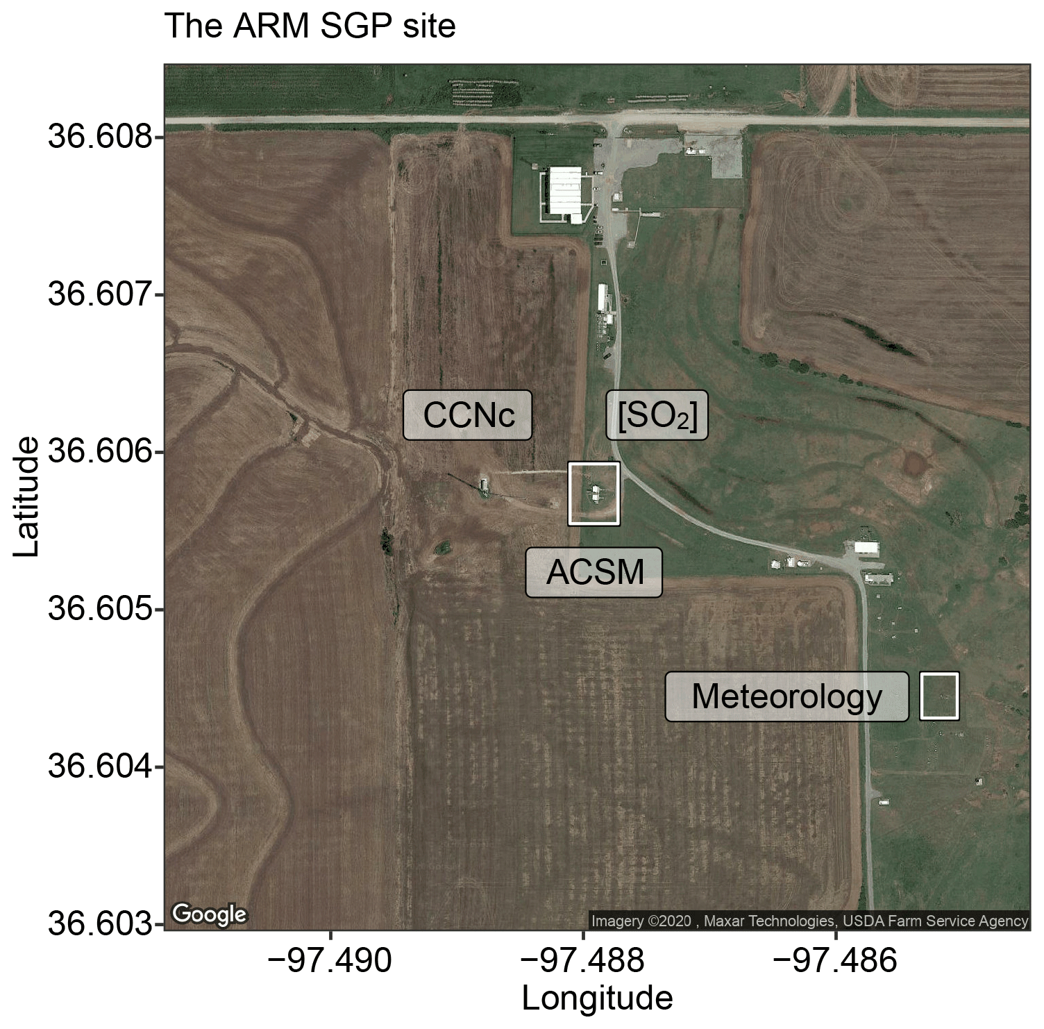
Figure 1 The ARM SGP site in Lamont, Oklahoma, USA, with marked locations of the instruments. Legend: meteorology – temperature and relative humidity measurements from the ARM Surface Meteorology Systems (MET) (Holdridge and Kyrouac, 1993; Chen and Xie, 1994); ACSM – Aerodyne Aerosol Chemical Speciation Monitor (Ng et al., 2011); [SO₂] – concentrations of SO₂ measured by the ARM Aerosol Observing System (AOS; Hageman et al., 1996); CCNc – cloud condensation nuclei particle counter (CCNc) (Shi and Flynn, 2007; Smith et al., 2011a, b; Hageman et al., 2017). This image is adapted from satellite imagery © 2020 Maxar Technologies, USDA Farm Service Agency obtained through the Google Maps Static API.

2.4.1 [CCN0.4] measurements

[CCN0.4] measurements at this SGP site have been made from 2007 to the present using a cloud condensation nuclei particle counter (CCNc) developed by Roberts and Nenes (2005) with technical details in Uin (2016). The CCNc is a continuous-flow thermal-gradient diffusion chamber for measuring aerosols that can act as CCN. To measure these, aerosol is drawn into a column, where well-controlled and quasi-uniform centerline supersaturation is created. Through software controls, the temperature gradient and flow rate are modified to vary (0.1 %–3 %) supersaturations and obtain CCN spectra. Water vapor condenses on CCN in the sampled air to form droplets, just as cloud drops form in the atmosphere; these activated droplets are counted and sized by an optical particle counter (OPC).

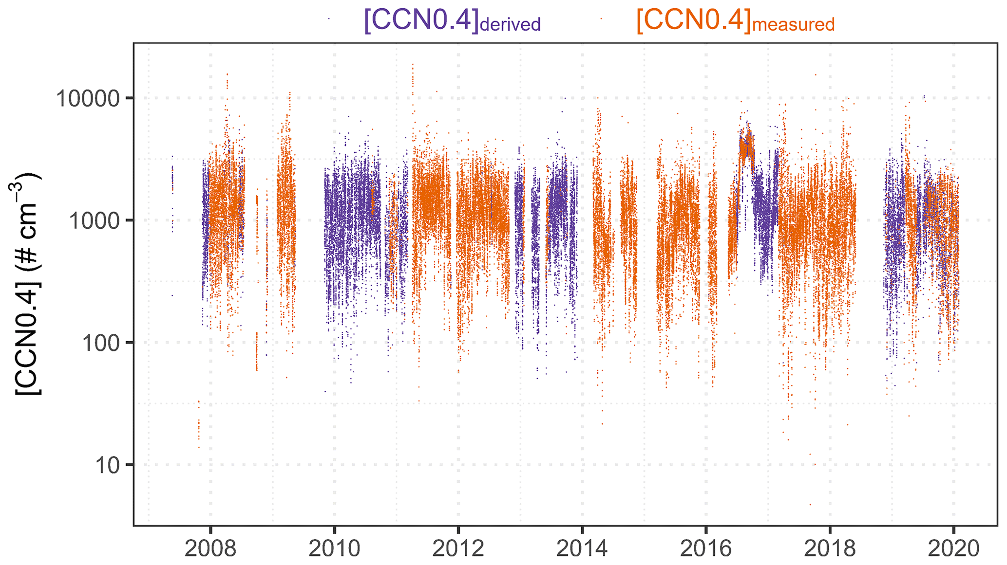
We integrate the quality-checked data (Shi and Flynn, 2007; Smith et al., 2011a, b; Hageman et al., 2017) made publicly available through ARM from co-located instruments at the SGP site to form a long-term record of [CCN0.4] as in Fig. 2 and for later analysis and validation of the RFRM.

Figure 2 Hourly [CCN0.4] measurements at Lamont, Oklahoma, from 2007 to 2020. The orange circles show the data for [CCN0.4] measured here. The purple circles show the data for [CCN0.4] derived from [CCN0.2–0.6] according to the method described in Sect. 2.4.2.

2.4.2 Filling the [CCN0.4] measurement gaps

The temporal range of available observations for [CCN0.4] at the SGP site is 19 May 2007 17:00:00 to 29 January 2020 23:00:00. For this period of 111 319 h, there is only ≈42 % data completeness. To improve the data coverage, we examine the possibility of using [CCN] for other reported supersaturation ratios (0.2 %–0.6 %).

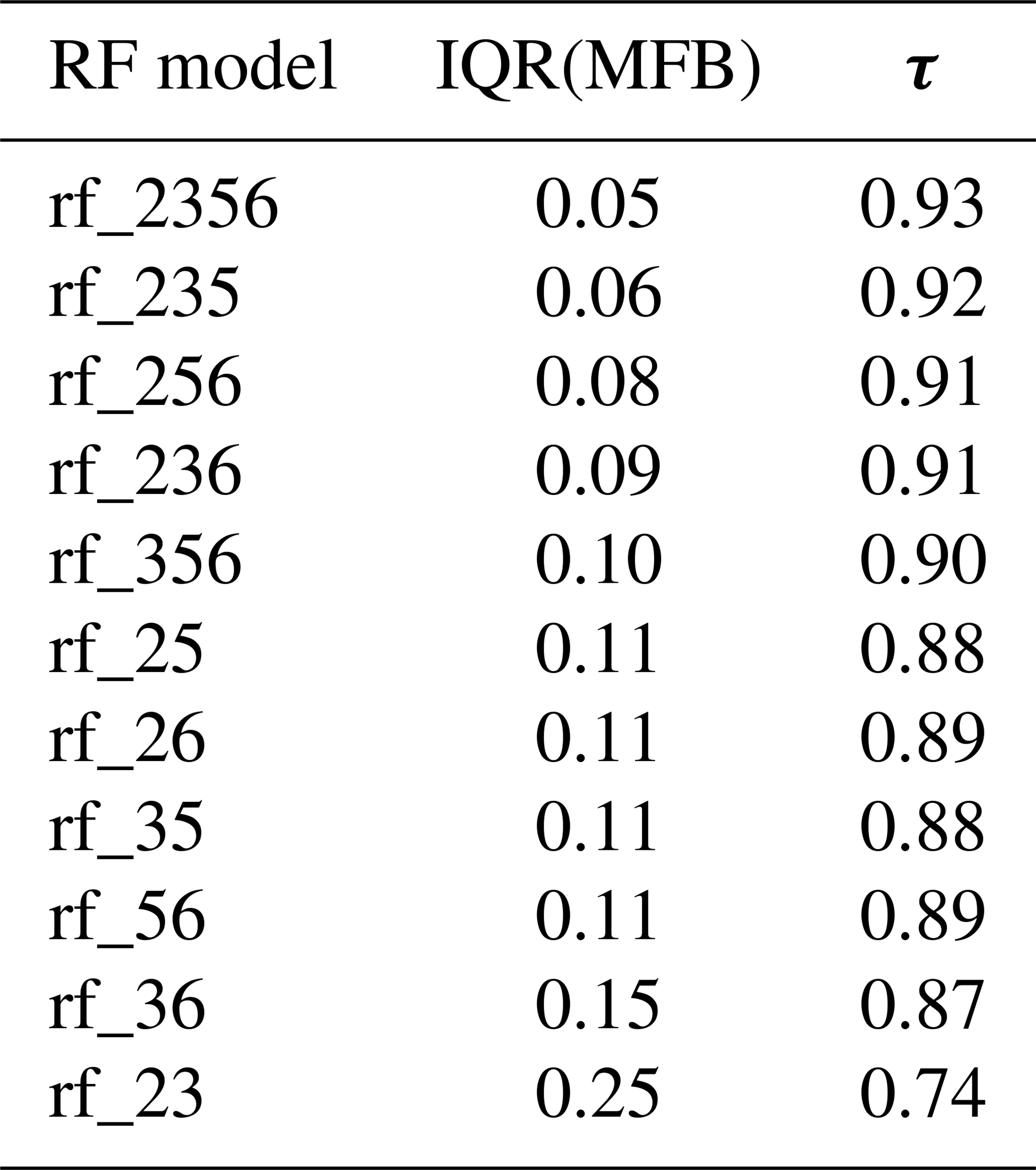
In a sneak preview of the efficacy of random forest for regression, we train random forest models that output [CCN0.4] from [CCN0.2–0.6]. These models are listed in Table 1, with the notation rf_n, where n denotes the supersaturations used as input (for instance, rf_356 indicates [CCN0.3], [CCN0.5], and [CCN0.6] were used as inputs to derive [CCN0.4]). The approach works exceptionally well and shows the potential for application with other datasets to fill in such gaps as well as to perform sanity checks on available data. As reported in Table 1, there is high correlation (Kendall's τ) and minimal deviation (interquartile range of mean fractional bias (IQR(MFB)) between random forest derived [CCN0.4] and measured [CCN0.4], when simultaneous data for [CCN0.4] are available.

Using this approach, we fill in the missing observations and improve data completeness from ≈42 % to ≈66 %, an increase of ≈54 %, for [CCN0.4] during this period (see Fig. 2).

Table 1 Evaluation metrics of the random forest models developed to derive [CCN0.4] from other supersaturations.

2.4.3 Atmospheric state and composition measurements

Meteorological data are sourced from the ARM Surface Meteorology Systems (MET) (Holdridge and Kyrouac, 1993) with technical details in Ritsche (2011). We use the ARM Best Estimate Data Products (ARMBEATM; Chen and Xie, 1994) derived from Holdridge and Kyrouac (1993) when available (1994–2016).

Trace gas concentrations are obtained from the ARM Aerosol Observing System (AOS; Hageman et al., 1996) with technical details in Jefferson (2011). Unfortunately, at the SGP site, measurements (Springston, 2012) are available only for [SO₂] from 2016 to the present. To compensate for this, we use data from the United States Environmental Protection Agency (EPA) Air Quality System (AQS) made publicly available at https://www.epa.gov/air-data (last access: 20 August 2020) from monitors in the vicinity (<100 km) of the SGP site.

Real-time aerosol mass loadings and their chemical composition measurements have been made from 2010 to the present using an Aerodyne aerosol chemical speciation monitor (ACSM; Ng et al., 2011) with technical details in Watson (2017). We use the aerosol chemical speciation data (Watson et al., 2018; Kulkarni, 2019; Behrens et al., 1990), which are publicly available through ARM.

For observation–model simultaneity, all data (atmospheric state, composition, and [CCN0.4]) are integrated to the hourly resolution with their geometric mean.

3 Results and discussion

3.1 RFRM: training, testing, and optimizing

The GCAPM output for 47 sites across the globe, for six selected vertical levels from surface to ≈ 8 km and for 30 years (1989–2018) at the half-hour time step (≈ 150 million rows, i.e., sets of predictors and [CCN0.4]) is considered in training the RFRM. The predictors of importance in controlling [CCN0.4] are listed in Table 2. The RFRM is trained on a subset of this data. First, the ARM SGP site is ignored; this is to establish a completely independent analysis with available observational data in Sect. 3.2.2. The remaining GCAPM data for 46 sites and six vertical levels each are partitioned into training (≈ 101 million rows) and testing sets (≈ 44 million rows) in a 7:3 ratio. Due to the large number of training and testing examples, these sets are reduced to a 1 % random subset; it is ensured to be representative, with almost identical statistical properties, of the training datasets (Fig. 3).

Table 2 Selected atmospheric state and composition variables as RFRM predictors for [CCN0.4].

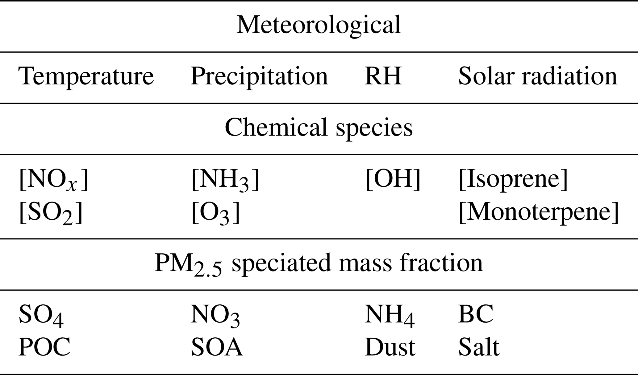
Figure 3 Scaled Gaussian kernel density estimate for [CCN0.4] for the training set (dark purple) and each of its subsets (10 %: light purple; 1 %: light orange; 0.1 %: dark orange). The distributions are almost identical. A 1 % randomly sampled subset is used to train the RFRM.

Once the data have been selected to train the RFRM, we tune the hyperparameters, which govern the training of the machine learning model. The default implementation of Wright and Ziegler (2017) comes with reasonable (balancing speed and accuracy) choices for these. Based on literature review (Probst et al., 2019, and references therein) as well as our preliminary examination of RFRMs with varying hyperparameters, we identify the following as most important to optimize: numtrees – number of trees in the forest; mtry – the minimum number of variables to consider for each split; and min.node.size – the minimum node size, i.e., the minimum size of homogeneous data to prevent overfitting. By setting the minimum number of training examples in the terminal nodes of the component trees of the RF, the individual tree depth is controlled, which further mitigates the overfitting associated with decision tree algorithms (discussed in Sect. 2.2). The default hyperparameter values in Wright and Ziegler (2017) are as follows: numtrees = 500, mtry = rounded-down square root of the number of variables, and min.node.size = 5. We verify whether these hyperparameter choices are optimal by performing a grid search of the hyperparameters and training multiple random forest models and not just examining their performance with the training set but also additionally with the test set. By evaluating the RFRMs with the test set (data that the machine learning algorithm was not exposed to during its training), additional mitigation of possible overfitting is achieved. Figures 4 and 5 show the results of this exercise.

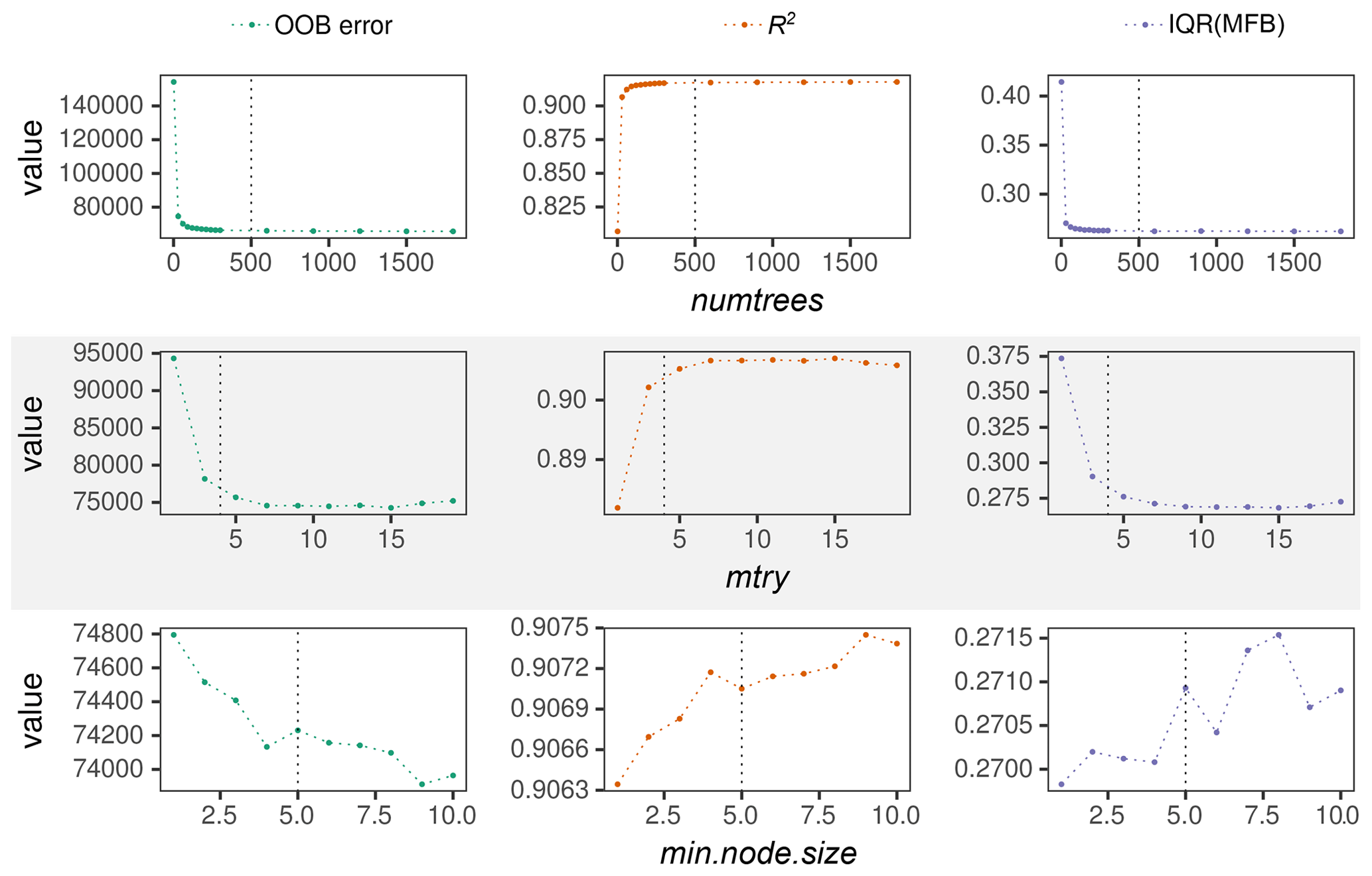
Figure 4 RFRM evaluation through OOB error (green), R² (orange), and IQR(MFB) (purple) with varying hyperparameters. The hyperparameters are (from top to bottom): numtrees, mtry, and min.node.size. Default hyperparameters for each trained model are as follows: numtrees = 500, mtry = 4, and min.node.size = 5 – also shown with the vertical black dotted lines when the corresponding default value has been varied.

Figure 4 has nine panels, as follows from top to bottom:

• the top three are for varying number of trees in the random forest: numtrees from 1 (a single decision tree) to 1800, through the default choice of 500 (marked with vertical black dotted line);

• the middle three are for varying number of variables considered at each split point: mtry from 1 to 19, through the default choice of 4 (marked with vertical black dotted line); and

• the bottom three are for varying minimum size of the terminal nodes: min.node.size from 1 to 10, through the default choice of 5 (marked with vertical black dotted line).

From left to right, the panels are as follows:

• the left three (green) show the overall out-of-bag error, i.e., the mean square error for the entire random forest computed using the complement of the bootstrapped data used to train each tree;

• the middle three (orange) show the R² values indicating the explained variance by the random forest; and

• the right three (purple) show the interquartile range of the mean fractional bias of the random forest model when applied to the test set.

A single decision tree (left-most point in each of the top three panels of Fig. 4) is able to explain the variance (R²≈0.81) in [CCN0.4] through the predictors' variabilities and has an interquartile range in the MFB (which has a median of ≈0.004: not pictured as the symmetry of MFB means the median → 0) of 0.41, which corresponds to a deviation of $\approx \pm \mathrm{20}\mathit{\%}$. However, this is drastically improved when moving beyond a simple decision tree to even a small ensemble of 30 trees (R²≈ 0.91; IQR(MFB) ≈ 0.27), which plateaus (within a range of ± 0.0005) after ≈ 500 trees. The out-of-bag (OOB) error shows a similar trend. Growing a random forest of 500 trees with a min.node.size of 5, we see the effect of varying mtry in the middle three panels. Instead, keeping the mtry fixed at the default value of 4; the rounded down square root of the 19 predictor variables and the random forest performance metrics with varying min.node.size are shown in the bottom three panels. Figure 4 thus shows the possibility of improving the random forest derivation of [CCN0.4] by changing the default choices of Wright and Ziegler (2017) for this specific work. It must be kept in mind that a reasonable cutoff, beyond which there is imperceptible gain in performance at increased computational cost, should be considered.

The results shown in Fig. 4 motivate a zoomed-in hyperparameter grid search to choose the optimal (accurate and fast) RFRM. Figure 5 shows this for the best-performing random forest models with numtrees ranging from 600 to 1400, mtry from 6 to 18, and min.node.size from 3 to 6. While there is variability, it must be noted that the y axes range over 2 %, 0.2 %, and 2 % of the values of OOB error, R², and IQR(MFB), respectively. While, indeed, considering a larger (numtrees) forest is beneficial, considering the cost-to-benefit ratio, the hyperparameters we choose are a maximum number of 800 trees in the forest, 12 (mtry) variables randomly chosen at each split, a minimum node size of 3 as the only control on tree depth, and the splitting rule as the minimization of variance. With these hyperparameters, the random forest has IQR(MFB), R², and OOB error of ≈100.34 %, ≈99.93 %, and ≈100.56 % of the best-performing model for each hyperparameter, respectively.

3.2 What the model learns

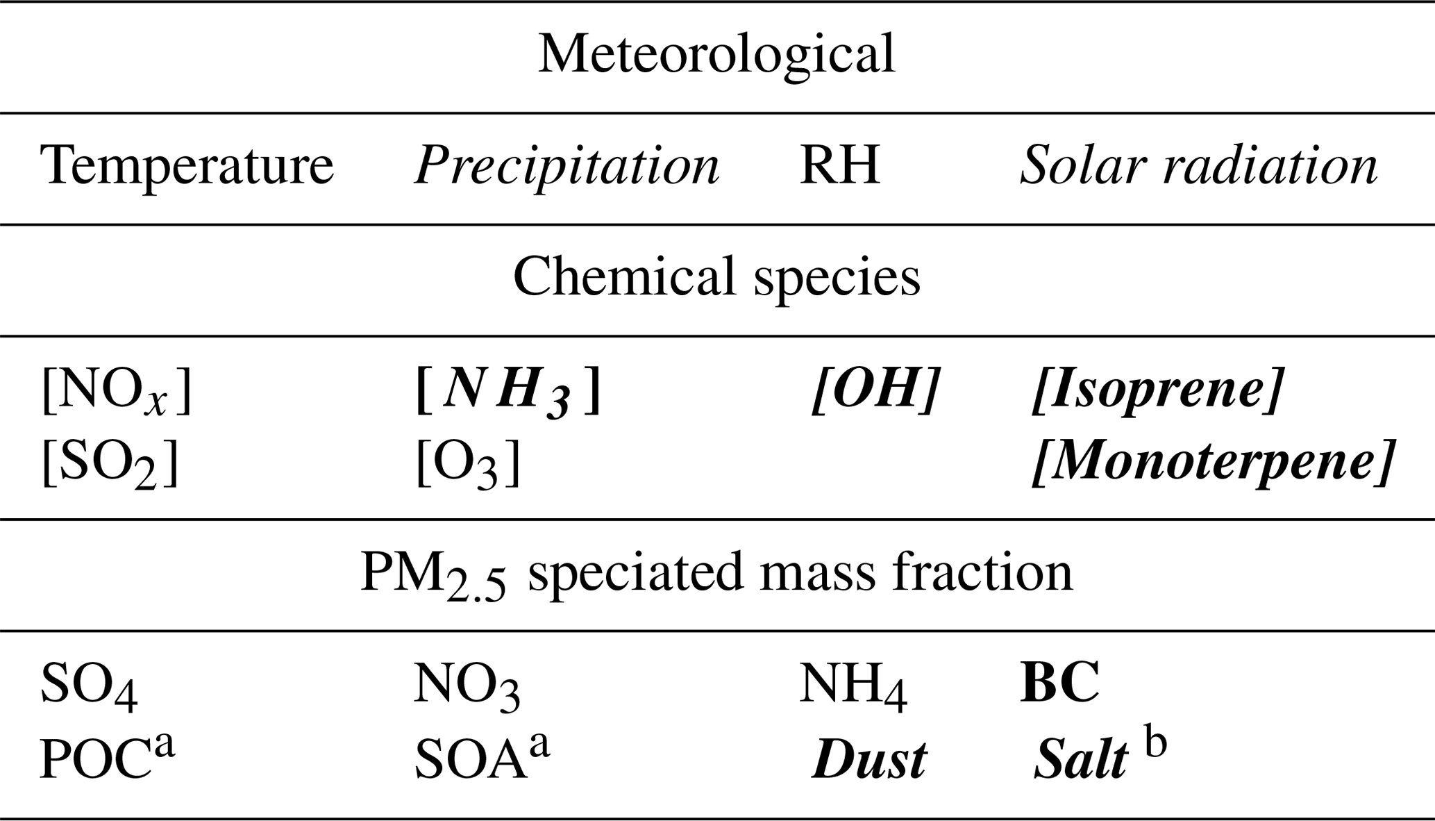
We train the optimized RFRM using the 19 predictors listed in Table 2 as predictors of [CCN0.4]; these are as follows: eight fractions of PM_2.5 (ammonium, sulfate, nitrate, secondary organic aerosol (SOA), black carbon (BC), primary organic carbon (POC), dust, and salt), seven gaseous species (nitrogen oxides (NO_x), ammonia (NH₃), ozone (O₃), sulfur dioxide (SO₂), hydroxyl radical (OH), isoprene, and monoterpene), and four meteorological variables (temperature, relative humidity (RH), precipitation, and solar radiation).

Figure 6 shows the importance of each predictor in determining the CCN0.4 number concentration in the above-trained RFRM. This importance measure is obtained by randomly permuting values of each predictor to break the association with CCN0.4. Also, the model is fed a pseudo-predictor of randomly generated white noise, labeled “Random” in Fig. 6. Most important are component mass fractions of PM_2.5, especially its inorganic fraction (ammonium, sulfate, and nitrate), [SO₂], the other PM_2.5 fractions excluding the salt and dust fractions, [NO_x], and [NH₃]. The Random predictor is least important, contributing imperceptibly to the [CCN0.4] prediction.

Figure 5 RFRM evaluation through OOB error (a), R² (b), and IQR(MFB) (c) with varying hyperparameters selected from the best balanced (accuracy and computational expense) ranges in Fig. 4.

Figure 6 Importance (in decreasing order) of each predictor in the RFRM derivation of [CCN0.4].

To quantify the importance of each of the 19 predictors, we do the following: (1) RFRM-Blind – train RFRMs without considering one variable at a time; (2) RFRM-Random – randomize each predictor variable and input into the RFRM. These exercises will provide a more robust, as well as more intuitive measure of the importance of each predictor by analyzing and comparing the deviation in predicted [CCN0.4] compared to the baseline optimized RFRM (hereafter, RFRM-AllVars). Table 3 shows the median ± median absolute deviation of MFB for each such trained RFRM-Blind and RFRM-Random evaluated with the test dataset, with the values for the baseline RFRM-AllVars at the bottom. For the MFB, its median absolute deviation (and even IQR(MFB)) is a stronger indicator of the performance than the median, due to the symmetry of MFB. Examining the median absolute deviation of the MFB, the “Blind” approach shows that the ammonium (PM_2.5NH₄), sulfate (PM_2.5SO₄), and secondary organic (PM_2.5SOA) fractions of PM_2.5 are most important (in increasing order) in determining [CCN0.4]. The Blind approach may, however, underestimate the importance of a predictor due to possible correlations with other predictors, as seen in Fig. 7. These cross correlations could mean the implicit participation of a predictor despite its absence in training the RFRM. To overcome this limitation, in the Random approach, the trained RFRM-AllVars is then input randomized predictors (one at a time) from the testing dataset. This breaks the association of each predictor with the outcome ([CCN0.4]) as well as with other predictors. The resulting change (if any) in the RFRM-AllVars would show the importance of the specific predictor. RFRM-Random for each predictor shows that all predictors (except solar radiation) are important, with the most important being PM_2.5SOA, PM_2.5SO₄, and PM_2.5NH₄.

Table 3 Mean fractional bias (MFB) of each random forest regression model (RFRM). RFRM-Blind refers to the RFRM trained ignoring the particular predictor. RFRM-Random refers to the randomization of the particular predictor before input into RFRM-AllVars. RFRM-AllVars (at the bottom of the table) is the baseline model where no variable is omitted or randomized. Values are median ± median absolute deviation of MFB.

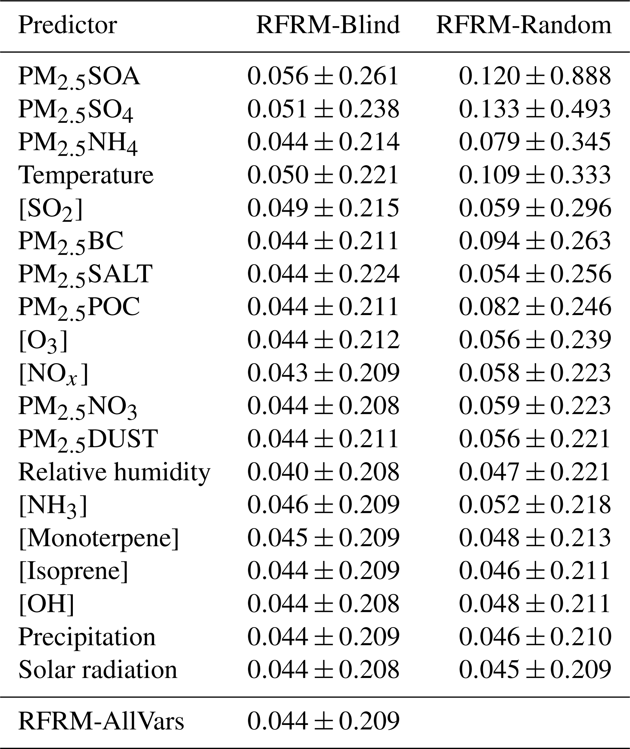
Table 3 thus shows the importance of each predictor towards determining [CCN0.4] in decreasing order, which complements the results in Fig. 6 that shows the out-of-bag increase in mean square error upon the permutation of a specific predictor. We modify the approach in Wright and Ziegler (2017) (a) to leverage the advantages of the MFB; (b) to account for any implicit correlations between the data used to train (bagged) and evaluate (out-of-bag) the RFRM by using the unseen testing dataset; and (c) to dissociate the effects of cross correlations between predictors. The results of this modified evaluation of the RFRM are in Table 3. These exercises to probe into the working of the RFRM show that all of the predictors were deemed necessary to capture [CCN0.4] magnitude and variability. The most important predictors are the PM_2.5 speciated components, gases including [SO₂], [O₃], and [NO_x], and temperature and relative humidity.

3.2.1 Comparison with GCAPM [CCN0.4]

We examine the RFRM in further detail with the subset of data excluded for testing, i.e., for the sites that RFRM-AllVars has not been exposed to during its training. Figure 8a shows RFRM-AllVars derived [CCN0.4] against that simulated by GCAPM for all of the testing dataset. RFRM-AllVars predicted [CCN0.4] values are highly correlated with expected values from GCAPM, with a correlation of τ≈0.88 and highest density along the dashed black line in Fig. 8a denoting MFB = 0 or complete agreement. The dashed blue and red lines denote $-\mathrm{1}<\text{MFB}<+\mathrm{1}$; ≈99.69 % of the values are within this factor of 3 times deviation. The dotted lighter blue and red lines denote $-\mathrm{0.6}<\text{MFB}<+\mathrm{0.6}$; ≈96.33 % of the values are within this range of good agreement between derived and expected [CCN0.4] values.

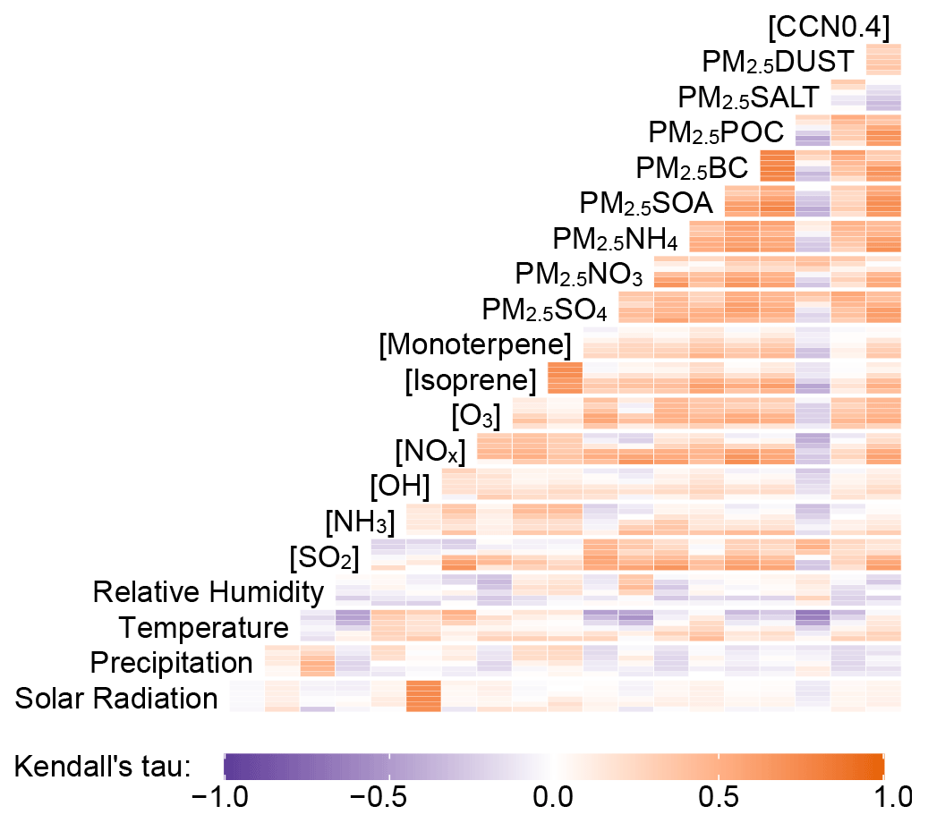
Figure 7 Kendall rank correlation (τ) for the 19 predictors and [CCN0.4] in the RFRM training dataset (≈101 million rows). The boxes show corresponding τ value according to color scale. Boxes are divided vertically to represent τ for each selected model height: surface, ≈ 1, ≈ 2, ≈ 4, ≈ 6, and ≈ 8 km.

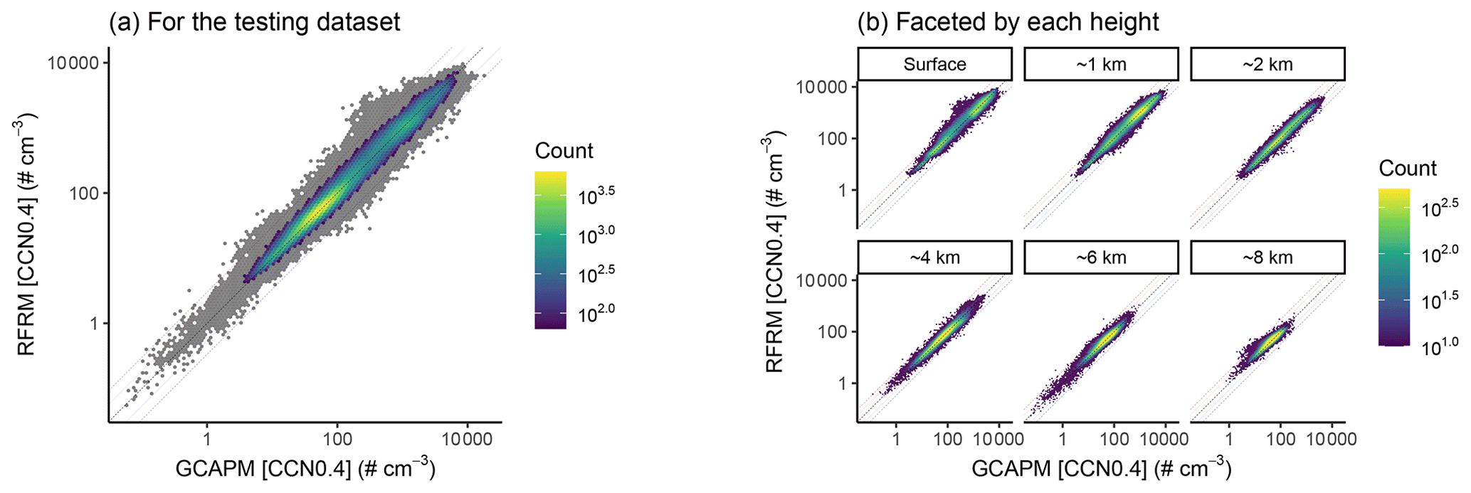
Figure 8 Binned scatterplot of RFRM versus GCAPM simulated [CCN0.4]. Color bar shows the counts of points in each hexagonal bin. Bins with low counts (<1 % of maximum count: ≈3 % of the data) are shaded gray. The lines indicate MFB of 0 (black; perfect agreement), +1 (darker red), −1 (darker blue), +0.6 (lighter red), and −0.6 (lighter blue).

Overall, the RFRM is able to derive [CCN0.4] with a median (median-absolute-deviation) MFB of 4.4(21) %. A comparison to expected [CCN0.4] values from GCAPM in Fig. 9 (a) by means of the MFB shows the robustness of RFRM-AllVars in greater detail. The highest density of MFBs is on or around 0, reiterating how well RFRM-AllVars predictions of [CCN0.4] compares to GCAPM simulated values.

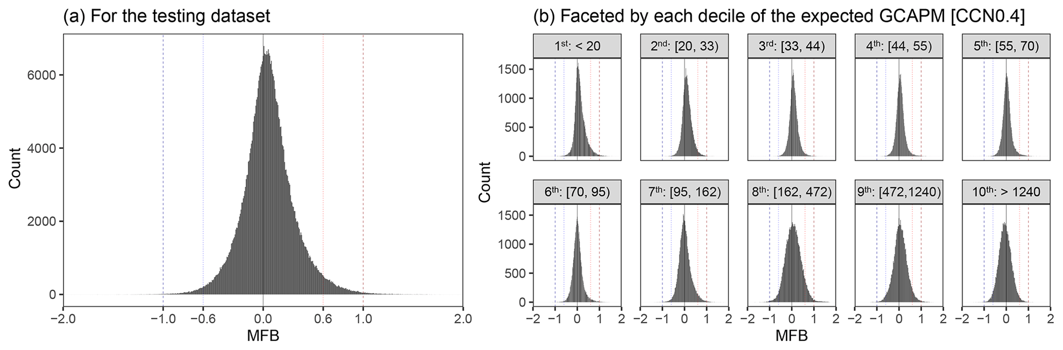
Figure 9 Mean fractional bias (MFB) of RFRM derived [CCN0.4] compared to expected values from GCAPM in the testing dataset (441 756 values). Histogram shows the counts of the pairs by MFB. The lines indicate perfect agreement (black), MFB of +1 (dashed red), and MFB of −1 (dashed blue). The dotted lines indicate MFB of +0.6 (dotted red) and −0.6 (dotted blue).

Figure 8a is faceted by height in Fig. 8b. Across the various heights, with varied [CCN0.4] ranges, RFRM-AllVars performs robustly with $\left|\text{MFB}\right|<\mathrm{2}$. Its robustness across varied [CCN0.4] ranges is further shown in Fig. 9b, where Fig. 9a is faceted by the deciles of the GCAPM simulated [CCN0.4]. RFRM-AllVars performs well over 4 orders of magnitude of [CCN0.4] from 10⁰ to $\mathrm{2.7}\times {\mathrm{10}}^{\mathrm{4}}{\mathrm{cm}}^{-\mathrm{3}}$.

3.2.2 Comparisons for the SGP site

We also examine the temporal trends of [CCN0.4] for the SGP site (the surface $\mathrm{2}{}^{\circ }\times {\mathrm{2.5}}^{\circ }$ model grid box), which was completely excluded from the RFRM training. Figure 10 shows the weekly-aggregated time series from 1989 to 2018 for (a) GCAPM simulated and (b) RFRM-AllVars derived [CCN0.4]. Also shown in Fig. 10d is the comparison, using MFB, of the derived [CCN0.4] of RFRM-AllVars versus the GCAPM [CCN0.4] values. The RFRM performs well, being able to capture weekly variations with good correlation (τ≈0.68) and low deviation (≈99.87 % within the good agreement range of $\left|\text{MFB}\right|<\mathrm{0.6}$).

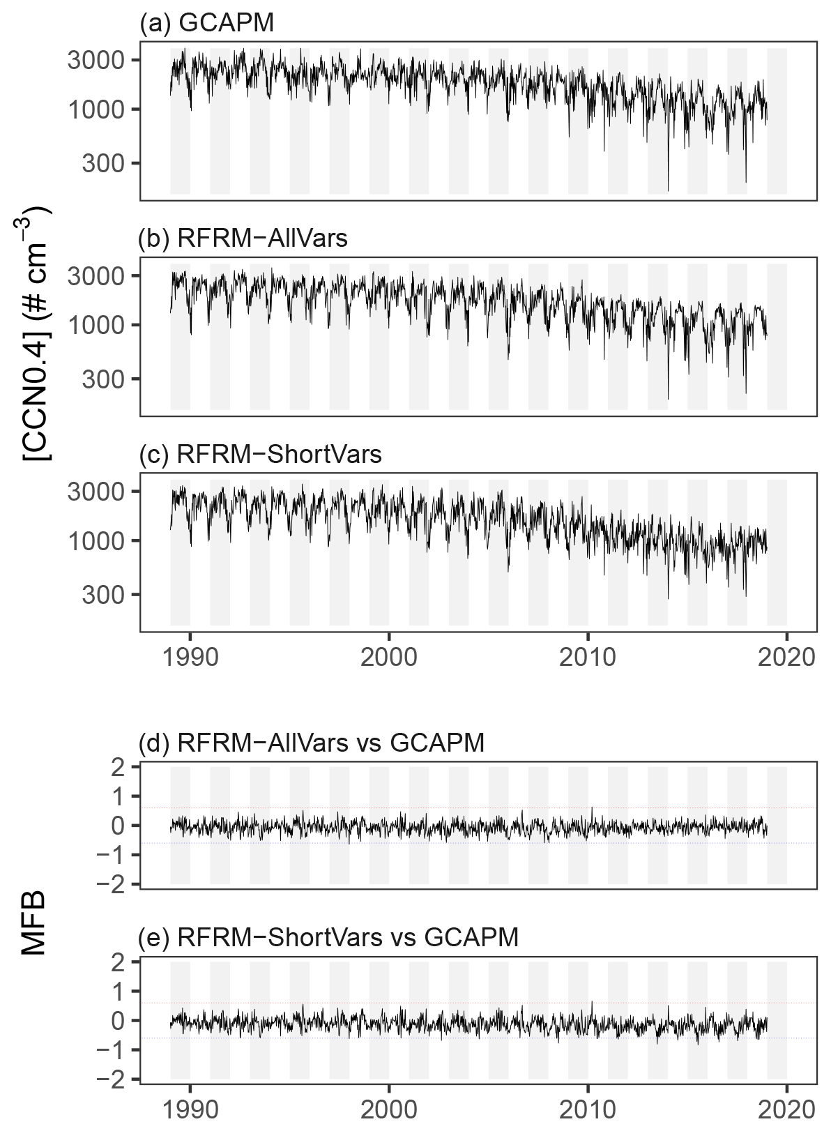
Figure 10 Time series (weekly-aggregated) for the surface $\mathrm{2}{}^{\circ }\times {\mathrm{2.5}}^{\circ }$ GCAPM grid box containing the SGP site – (a) GCAPM simulated, (b) RFRM-AllVars, and (c) RFRM-ShortVars derived [CCN0.4] – and the mean fractional bias (MFB) of (d) RFRM-AllVars and (e) RFRM-ShortVars. Dotted lines show the good agreement range of $\left|\text{MFB}\right|<\mathrm{0.6}$.

RFRM application: measured predictors as input

As detailed in Sect. 2.4, there are numerous observations of atmospheric state and composition for the SGP site that can be utilized to validate the RFRM with empirical data. In an ideal situation, continuous, long-term, high-quality measurements for all the inputs to the RFRM (the predictor variables listed in Table 2) would have aided in this analysis. However, due to the sparsity and absence of measurements of certain predictors, we are limited to the available factors listed in Table 4. These are shown in Fig. 11, with the speciated PM_2.5 predictors in Fig. 11a, the trace gas measurements in Fig. 11b, and the meteorological variables in Fig. 11c.

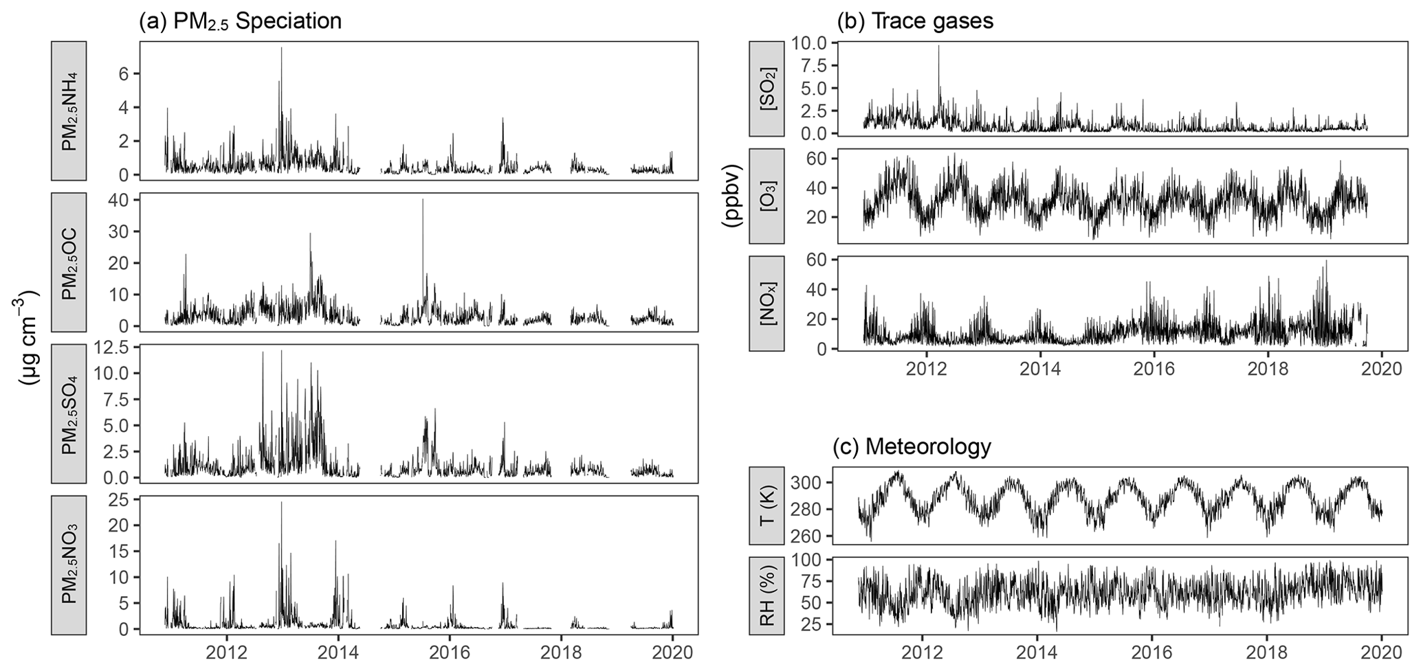
Figure 11 Time series (daily-aggregated) for predictors at the ARM SGP site: (a) PM_2.5 speciation; (b) trace gas; and (c) meteorological measurements.

Thus, with a reduction from 19 to 9 predictor variables, we retrain the RFRM to use only these as inputs to derive [CCN0.4]. The RFRM optimization is carried out as described in Sect. 2.2; the RFRM hyperparameters are numtrees=1000, mtry=3, and min.node.size=3 and use the nine predictors listed in Table 4 to derive [CCN0.4]. This retrained RFRM (henceforth, RFRM-ShortVars) is evaluated using the testing dataset; with median (median-absolute-deviation) MFB deteriorating from 0.044(0.209) to −0.184(0.382), 96.33 to 80.30 % of the derived [CCN0.4] values in the good agreement range, and correlation reducing from τ≈0.88 to 0.79. While RFRM-ShortVars is less robust compared to RFRM-AllVars, the statistical estimators of model performance are still high for RFRM-ShortVars.

Specifically for the SGP site, Fig. 10c and e show the weekly-aggregated RFRM-ShortVars derived [CCN0.4] and its comparison with the GCAPM [CCN0.4] values, respectively. RFRM-ShortVars performs well, being able to capture these variations with good correlation (τ≈0.66) and low deviation (≈98.72 % within the good agreement range).

Table 4 RFRM predictors for [CCN0.4] as listed in Table 2. Italicized text shows those predictors determined (in Sect. 3.2) to not strongly impact RFRM prediction of [CCN0.4]. Bold text shows the absence of their hourly measurements.

Note: ^a measurements for PM_2.5 POC and SOA are reported as PM_2.5 OC (total organic carbon). ^b For PM_2.5 salt, PM_2.5 chloride measurements are available but subject to a large percent of missing data.

Using measurements of the nine predictor variables at the SGP site for 2010–2020, we use the developed RFRM-ShortVars to derive [CCN0.4]. Compared to [CCN0.4] measurements, the RFRM performs well, with τ≈0.36 and ≈67 % with $\left|\text{MFB}\right|<\mathrm{0.6}$. We note that filling the measurement gaps (per Sect. 2.4.2) could contribute to this observed decrease in RFRM performance (from RFRM-AllVars → RFRM-ShortVars). However, this contribution is minimal: when comparing the RFRM-ShortVars-derived [CCN0.4] with measurements excluding the filled-in [CCN0.4], Kendall's τ correlation increased from 0.36 to 0.42 and the percentage within the good-agreement range from 67.02 % to 69.34 %, with the sample size n reducing from 39 811 to 29 047. The deteriorated performance is mainly due to the reduction in necessary predictors to the available ones; the uncertainties associated with the measurements themselves may compound this. Regardless, the variability from diurnal to decadal scales is captured by the RFRM (top-left panel in Fig. 12a) when compared to the measurements (bottom-left panel in Fig. 12a) of [CCN0.4]. For reference, in Fig. 12a the top-right and bottom-right panels are the same as in Fig. 10c and a, respectively, but for this period of measurements.

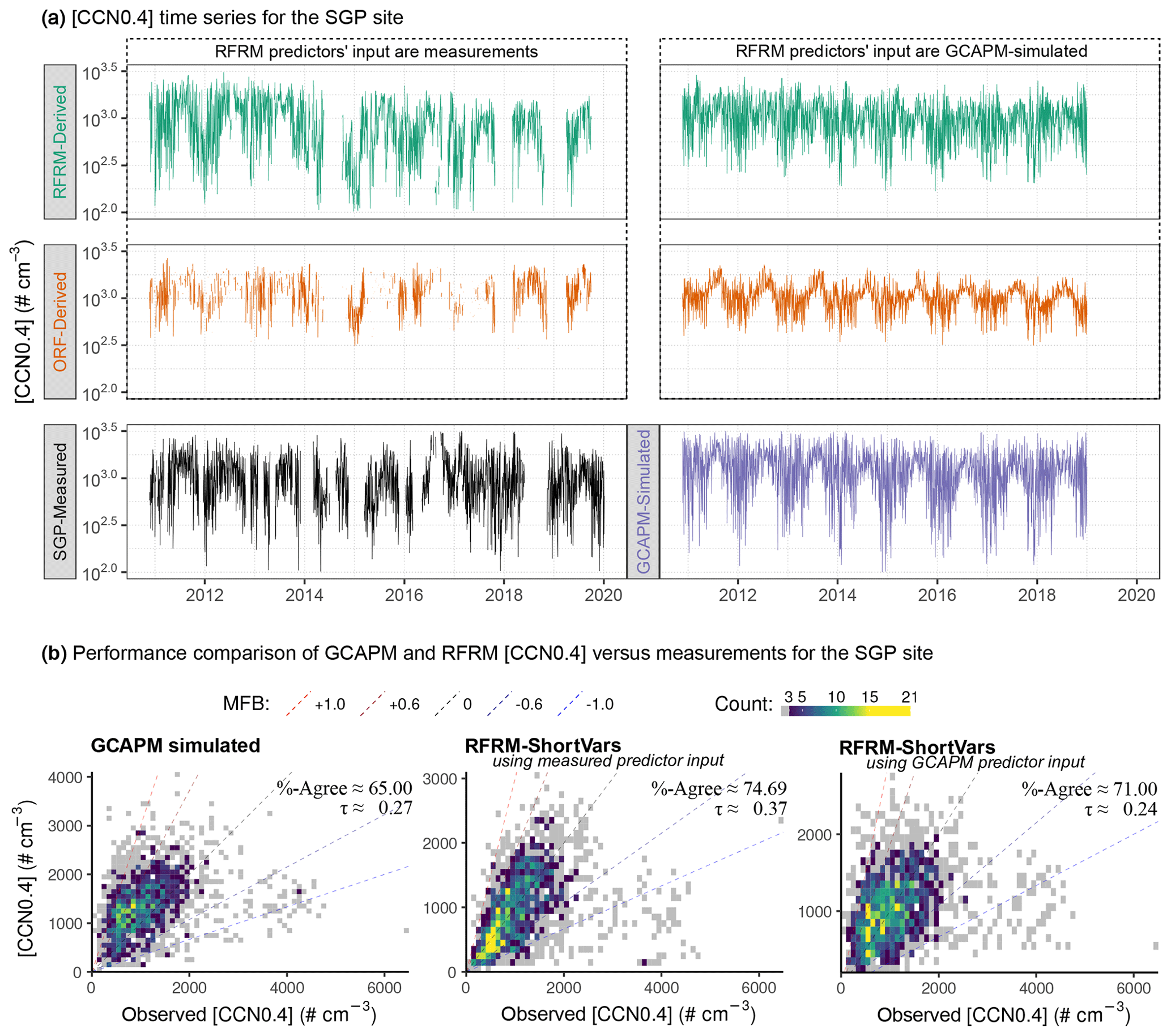
Figure 12 (a) Time series (daily-aggregated) for [CCN0.4] derived by RFRM-ShortVars (top two) and ORF (middle two), compared to SGP measured (bottom-left) and GCAPM-simulated (bottom-right). (b) Performance comparison of the models in quantifying [CCN0.4] compared to its measured values for the SGP site: left – GCAPM; center – RFRM-ShortVars with measurements of predictors as input; right – RFRM-ShortVars with GCAPM-simulated predictors as input. The summary performance metrics are τ: Kendall's rank correlation coefficient and %-Agree: the percentage of pairwise model–observation compared values within the good-agreement range defined as $-\mathrm{0.6}<\text{MFB}<+\mathrm{0.6}$.

Performance comparison of RFRM and GCAPM

Figure 12b compares GCAPM and RFRM performance in quantifying [CCN0.4] for SGP with respect to its measurements corresponding to Fig. 12a. In the left-hand panel, GCAPM simulated [CCN0.4] shows fair correlation (τ≈0.27) with SGP measurements and 65 % within the good-agreement range. The general tendency is overestimation (median MFB≈0.25), seen as higher density above the perfect agreement line (dashed black). RFRM-ShortVars derives [CCN0.4] (Fig. 12b: center) to a greater degree of agreement than GCAPM does, with τ≈0.37 % and ≈75 % with $\left|\text{MFB}\right|<\mathrm{0.6}$ and $\text{median MFB}\approx -\mathrm{0.04}$ indicating a slight tendency to underestimate.

It is to be recalled that the GCAPM [CCN0.4] is more reflective of regional tendencies, simulating [CCN0.4] for a $\mathrm{2}{}^{\circ }\times {\mathrm{2.5}}^{\circ }$ grid box around the SGP site. The RFRM is trained on GCAPM, from where the associations were learned between atmospheric state and composition variables and [CCN0.4], thus implicitly imbibing the effect of physical and chemical processes that control particle number concentrations. That RFRM-ShortVars-derived [CCN0.4] is better representative is a demonstration that these processes are well-represented within GCAPM. Leveraging this aspect as well as utilizing localized conditions (actual measurements) of atmospheric state and composition, the RFRM performs significantly better than GCAPM. These results and the ability to capture the variability of [CCN0.4] across temporal scales demonstrate the derivation of [CCN0.4] through the more commonly available measurements of meteorology: atmospheric chemical species including speciation of particulate matter.

The right-hand panel of Fig. 12b shows how RFRM-ShortVars performs when using GCAPM simulated values of the input predictor variables. τ≈0.24 and 71 % with $\left|\text{MFB}\right|<\mathrm{0.6}$ indicates that the RFRM model performance is comparable to GCAPM for the SGP site in alignment with our observations in Sect. 3.2.1. This is encouraging towards further development of this machine learning approach for potential application in Earth system models (ESMs). The random forest technique discussed here has two key virtues: (1) its computational advantages as discussed in Sect. 2.2 and (2) its learning from a state-of-the-science chemical transport model coupled with size-resolved microphysics. In ESMs, where the demand for computational efficiency results in using simplified bulk microphysical treatment, the RFRM can provide a more accurate representation of particle numbers, especially those that mediate aerosol–cloud interactions, while remaining computationally efficient.

RFRM trained using measurements

Development of the machine learning model generally requires a large number of training examples; however, we also investigate the possibility of developing an RFRM with the measurement data alone. The RFRM optimization is carried out as described in Sect. 2.2; this RFRM trained on actual measurements at SGP has numtrees =1000, mtry=3, and min.node.size=5. Compared to the RFRM trained on GCAPM simulated data (≈ 150 million training examples), such an RFRM has only ≈ 34 000 training examples for the SGP site. We train such an RFRM, henceforth denoted as ORF (observation-based random forest regression model), and examine its performance.

In comparison with SGP measured [CCN0.4], ORF shows correlation of τ≈0.53 and good agreement with ≈81.22 % of its derived [CCN0.4] values. The time series (daily-aggregated) of ORF-derived [CCN0.4] is shown in Fig. 12a, with measured predictors as input to the RFRM in the middle-left panel and GCAPM predictors as input to the RFRM in the middle-right panel. In Fig. 13b ORF-derived [CCN0.4] is compared to hourly measurements. ORF appears to perform better than RFRM-ShortVars from the summary statistics. However, it is unable to capture the range of variations in magnitude (middle-left panel in Fig. 12a). Similar results are observed (Figs. 13d and 12a middle-right) when ORF is applied to GCAPM simulated data. This exercise of developing an observation-based RFRM is, however, not technically justifiable due to the small number of training examples and applicability to only the SGP site. Regardless, this exercise provides insight into whether considering only 9 out of the 19 required predictor variables is sufficient for RFRM-ShortVars, an examination of which suggests the affirmative. Further, this exercise is insightful in demonstrating the unlikelihood of missing any important predictor in the RFRM, providing an additional check on the importance of the RFRM predictors, and the potential utility of this machine learning approach being trained directly, without a physicochemically informed model, on atmospheric state and composition measurements to derive [CCN0.4].

Figure 13 Mean fractional bias (MFB) of the random forest derived [CCN0.4] compared to expected values. (a, b) Comparison with measured [CCN0.4]. (c, d) Comparison with GCAPM simulated [CCN0.4]. The histograms show the pairwise counts (total is inset top-left in each panel) by MFB. The lines indicate MFB of 0 (black), +1 (dashed red), −1 (dashed blue), +0.6 (dotted red), and −0.6 (dotted blue). The percentage of RFRM derived values in good ($\left|\text{MFB}\right|<\mathrm{0.6}$) and fair ($\left|\text{MFB}\right|<\mathrm{1}$) agreement are shown close to the +0.6 and +1.0 MFB lines, respectively.

4 Summary

We develop an RFRM to predict the number concentrations of cloud condensation nuclei at 0.4 % supersaturation ([CCN0.4]) from atmospheric state and composition variables. This RFRM, trained on 30-year simulations by a chemical transport model (GEOS-Chem) with a detailed microphysics scheme (APM), is able to predict [CCN0.4] values. The RFRM learns that the PM_2.5 fractions (except salt and dust) and gases such as SO₂ and NO_x are the most important determinants of [CCN0.4]. The RFRM is robust in its derivation of [CCN0.4], with a median (median-absolute-deviation) mean fractional bias of 4.4(21) % with 96.33 % of the derived values within the good agreement range ($\left|\text{MFB}\right|<\mathrm{0.6}$) and strong correlation of Kendall's τ≈0.88 for various locations around the globe, at various altitudes in the troposphere, and across a varied range of [CCN0.4] magnitudes. We also demonstrate the application of this technique for deriving [CCN0.4] from measurements of [CCN] at other supersaturations. For a location in the Southern Great Plains region of the United States, using real measurements as input to the RFRM demonstrates its applicability. To use the measurement data as input to the RFRM required its tweaking to account for unavailable measurements for certain predictors. The truncated RFRM performs robustly despite these adjustments: median (median-absolute-deviation) MFB of −18(38) % with 80.30 % of the derived [CCN0.4] in good agreement and strong correlation of Kendall's τ≈0.79. Specifically for the ARM SGP site, using measured predictors as input to the RFRM and comparison with measured [CCN0.4], the median (median-absolute-deviation) MFB is −6(61) % with 67.02 % of the derived [CCN0.4] in good agreement and Kendall's correlation coefficient τ≈0.36.

4.1 Further discussion and outlook

There are a number of limitations in the application of the present study to augment empirical measurements of [CCN]. These are as follows:

• The RFRM is trained on GCAPM, with the assumption that the physical and chemical processes that relate the “predictor” variables to the [CCN0.4] outcome are accurate. Previous studies show that GCAPM performs reasonably when compared to observations, but uncertainties in both model and observation may contribute to uncertainties in the RFRM derivation.

• Co-located and simultaneous (with [CCN0.4] measurements) measurements of the required predictor variables were available only for certain predictors. We had to retrain the RFRM to account for these constraints, which sacrificed its accuracy in deriving [CCN0.4]. Other issues with measurements arise from the limitations of their accuracy, precision, and detection limits. Further sources of error are the utilization of predictor measurements from nearby (but not co-located) monitors to fill in significant gaps in the required data for the SGP site.

• Random forest was the machine learning tool of choice due to its parallelizability and high degree of accuracy. There are, however, other tools such as XGBoost (a choice for many winners of machine learning competitions) or regression neural networks. These, among others, could offer improved [CCN0.4] derivation. A cursory examination for the present study, however, showed no significant improvement at the cost of much higher computational expense.

• To overcome some of the gaps in the [CCN0.4] measurement data from the SGP site, we proposed and implemented a derivation of [CCN0.4] from [CCN] measurements at other supersaturations using the random forest technique. While this derivation was confirmed to be exceptionally good, this is an approximation.

• Development of an observation-based RFRM is presented in this study. However, it can be significantly improved with more observations for the SGP site, and generalizable if trained with observations from numerous other sites. This was presently not possible.

Despite the caveats associated with this work, this proof of concept shows promise for wide-ranging development and deployment. This machine learning approach can provide improved representation of cloud condensation nuclei numbers:

• in locations where their direct measurements are limited, but measurements of other atmospheric state and composition variables are available. Typically, since measurements of PM_2.5 speciation, trace gases, and meteorology are easier than those of [CCN0.4], there are longer and more widely (spatially) distributed in situ measurement records, especially through air quality monitoring networks. The developed RFRM can derive [CCN0.4] from these ubiquitous measurements to complement [CCN0.4] measurements when available and fill in the gaps in their absence.

• in Earth system models:

  • by providing a more accurate alternative to bulk microphysical parameterizations

  • by providing a computationally less intensive alternative to explicit bin-resolving microphysics models.

This work is an initial step towards fast and accurate derivation of [CCN0.4], in the absence of its measurements, constrained by empirical data for other measurements of atmospheric state and composition. This work demonstrates the possible applications of machine learning tools in handling the complex, nonlinear, ordinal, and large amounts of data in the atmospheric sciences.