the Creative Commons Attribution 4.0 License.
the Creative Commons Attribution 4.0 License.
 | 04 Nov 2020
Emission of biogenic volatile organic compounds from warm and oligotrophic seawater in the Eastern Mediterranean
Chen Dayan
Pawel K. Misztal
Maor Gabay
Alex B. Guenther
Biogenic volatile organic compounds (BVOCs) from terrestrial vegetation and marine organisms contribute to photochemical pollution and affect the radiation budget, cloud properties and precipitation via secondary organic aerosol formation. Their emission from both marine and terrestrial ecosystems is substantially affected by climate change in ways that are currently not well characterized. The Eastern Mediterranean Sea was identified as a climate change “hot spot”, making it a natural laboratory for investigating the impact of climate change on BVOC emissions from both terrestrial and marine vegetation. We quantified the mixing ratios of a suite of volatile organic compounds (VOCs), including isoprene, dimethyl sulfide (DMS), acetone, acetaldehyde and monoterpenes, at a mixed vegetation site ∼4 km from the southeastern tip of the Levantine Basin, where the sea surface temperature (SST) maximizes and ultra-oligotrophic conditions prevail. The measurements were performed between July and October 2015 using a proton transfer reaction time-of-flight mass spectrometer (PTR-ToF-MS). The analyses were supported by the Model of Emissions of Gases and Aerosols from Nature (MEGAN v2.1). For isoprene and DMS mixing ratios, we identified a dominant contribution from the seawater. Our analyses further suggest a major contribution, at least for monoterpenes, from the seawater. Our results indicate that the Levantine Basin greatly contributes to isoprene emissions, corresponding with mixing ratios of up to ∼9 ppbv several kilometers inland from the sea shore. This highlights the need to update air quality and climate models to account for the impact of SST on marine isoprene emission. The DMS mixing ratios were 1 to 2 orders of magnitude lower than those measured in 1995 in the same area, suggesting a dramatic decrease in emissions due to changes in the species composition induced by the rise in SST.
- Article
(3957 KB) - Full-text XML
-
Supplement
(18059 KB) - BibTeX
- EndNote


Biogenic volatile organic compounds (BVOCs) emitted from terrestrial vegetation and marine organisms significantly affect air pollution and health via increasing regional photochemical O3 pollution (Curci et al., 2009), enhancing local O3 removal via chemical reaction (Calfapietra et al., 2013) and serving as precursors for secondary organic aerosol (SOA) formation (Griffin et al., 1999; Lang-Yona et al., 2010; Ren et al., 2017). Considering the large global emission rate of BVOCs mostly from terrestrial vegetation (700–1000 TgC yr−1; Laothawornkitkul et al., 2009), biogenic SOA formation further impacts the radiation budget, precipitation and climate (Chiemchaisri et al., 2001; Wuebbles et al., 1989). BVOC oxidation likewise increases CO2 levels, as a direct product, and methane concentrations, by reducing the oxidation capacity (Penuelas et al., 2010).
Only a relatively minor fraction of all BVOCs (>10 000) are known to have sufficient reactivity and emissions to play an important role in climate and photochemistry (Guenther, 2002). Here, we focus on some of the important emitted reactive BVOCs, including 2-methyl-1,3-butadiene (isoprene), dimethyl sulfide (DMS) and some oxygenated volatile organic compounds (VOCs). The emission of isoprene from vegetation has received a lot of attention in recent years because this compound has the highest global emission rates among all reactive BVOCs from vegetative sources (Guenther, 2002) and due to its high photochemical reactivity and contribution to SOA amounts, estimated to be at least 27 %–48 % of total global SOA formation (Carlton et al., 2009; Meskhidze and Nenes, 2007). It is also well recognized that isoprene is also emitted from seawater (Bonsang et al., 1992; Goldstein and Galbally, 2007; Kameyama et al., 2014; Liakakou et al., 2007; Matsunaga et al., 2002), by marine organisms, including phytoplankton, seaweeds and microorganisms (Alvarez et al., 2009; Broadgate et al., 2004; Kameyama et al., 2014; Kuzma et al., 1995). Although the emission rates of isoprene into the marine boundary layer (MBL) are estimated to be substantially lower than terrestrial emissions, 0.1–1.9 TgC yr−1 (Arnold et al., 2009; Palmer and Shaw, 2005) vs. 400–750 TgC yr−1 (Arneth et al., 2008; Guenther et al., 2006, 2012), they play an important role in SOA formation (Hu et al., 2013) and photochemistry (Liakakou et al., 2007) in the marine environment, particularly in more remote areas (Ayers et al., 1997; Carslaw et al., 2000).
DMS is another important source for SOA formation and for atmospheric sulfur. The DMS emission rate is much higher from seawater than from terrestrial vegetation because the marine environment contains different types of phytoplankton, algae and microbial activity (Gage et al., 1997; Stefels et al., 2007; Vogt and Liss, 2009). DMS emission in the MBL is estimated at 15–34.4 Tg yr−1 (Kettle and Andreae, 2000; Lana et al., 2011), the largest natural source of sulfur in the atmosphere (Andreae, 1990; Simo, 2001), accounting for nearly half the total sulfur emissions in the atmosphere (Dani and Loreto, 2017).
Oxygenated VOCs, including aldehydes, alcohols, ketones and carboxylic acids, can induce tropospheric O3 formation via alkylperoxy formation (Monks et al., 2015; Müller and Brasseur, 1999; Singh, 2004) and act as OH precursors, particularly in the upper troposphere (Lary and Shallcross, 2000; Singh et al., 1995; Wennberg et al., 1998). Similar to isoprene and DMS, oxygenated VOCs serve as precursors to SOA formation (Blando and Turpin, 2000).
The emission of BVOCs from both terrestrial and marine sources is fundamentally influenced by climate changes. For instance, most BVOC emissions from terrestrial vegetation tend to increase exponentially with temperature (Goldstein et al., 2004; Guenther et al., 1995; Monson et al., 1992; Niinemets et al., 2004; Tingey et al., 1990), while drought can negate the effect of temperature on the emission rate from vegetation (Holopainen and Gershenzon, 2010; Llusia et al., 2015; Peñuelas and Staudt, 2010; Schade et al., 1999). Increases in seawater acidification and sea surface temperature (SST) significantly affect BVOCs in various ways, including by altering the biodiversity, spatial and temporal distribution, and physiological activity of marine organisms, influences that are currently not well characterized (Beaugrand et al., 2008, 2010; Bijma et al., 2013; Bopp et al., 2013; Dani and Loreto, 2017). Accordingly, the effect of climate change on BVOC emissions into the MBL is largely unknown (Boyce et al., 2010; Dani and Loreto, 2017).
The Eastern Mediterranean Basin region has been recognized as being highly responsive to climate change and has been aptly named a primary “climate change hotspot” (Giorgi, 2006; IPCC, 2007; Lelieveld et al., 2012). This makes it an attractive site to study the impact of anthropogenic stress and climate change on marine BVOC emissions. In addition, being oligotrophic, there is a predominance of unicellular and small plankton such as cyanobacteria (Krom et al., 2010) that can more efficiently perform CO2 fixation and utilize nutrients under such conditions, respectively (Fogg, 1986; Mazard et al., 2004). Moreover, the high SST tends to further shift the planktonic community toward an increase in unicellular and small plankton (Mazard et al., 2004; Rasconi et al., 2015).
At the southeastern tip of the Mediterranean Basin is the Levantine Basin, which is ultra-oligotrophic and the warmest region in the Mediterranean Sea (Shaltout and Omstedt, 2014; Azov, 1986; Krom et al., 2010; Psarra et al., 2000; Sisma-Ventura et al., 2017; Yacobi et al., 1995), particularly in its northern section (Efrati et al., 2013; Koçak et al., 2010). This region has experienced a significant increase in SST during the last decade ( ∘C yr−1; Ozer et al., 2016) with temperatures exceeding 30 ∘C 2 km from the coastline in 2015 (IOLR, 2015).
Most of the surface BVOC measurements of the Eastern Mediterranean are from Finokalia, Crete (Kouvarakis and Mihalopoulos, 2002; Liakakou et al., 2007). To the best of our knowledge, only a few measurements of BVOCs have been performed in the Levantine Basin, including BVOC emissions in Cyprus (e.g., Debevec et al., 2017; Derstroff et al., 2017) and DMS measurements in Israel (Ganor et al., 2000).
This study includes the first measurements of a suite of BVOCs near the Levantine Basin coast. The measurements were performed in a mixed Mediterranean vegetation shrubbery with the main objective being the study of the contribution of both seawater and local vegetation to the concentrations of key BVOCs, including isoprene, DMS, acetone, acetaldehyde and monoterpenes (MTs). A special focus was given to the effect of meteorological conditions on the contribution of each source to the measured concentrations.
2.1 Measurement site
Field measurements were performed in Ramat Hanadiv Nature Park (33∘33'19.87” N, 32∘56'50.25” E). The measurement site is situated at the edge of the park's memorial garden. This site is located about 3.6 km from the Mediterranean shore and is 120 m above sea level. The characteristics of the park have been detailed by Li et al. (2018) and are shown in Fig. 1. The nature park consists of mixed natural Mediterranean vegetation: Quercus calliprinos (∼25 %), Pistacia lentiscus (∼20 %), the sclerophyll Phillyrea latifolia (broad-leaved phillyrea) (∼7.5 %), invasive species (∼10 %), Cupressus (5 %), Sarcopoterium spinosum (∼2 %), Rhamnus lycioides (∼2 %) and Calicotome villosa (∼1 %). The park's western part features a few scattered Pinus halepensis (<5 %) combined with planted pine (Pinus halepensis and Pinus brutia) and cypress (Massada et al., 2012). During the measurements, the average canopy height was ∼4.5 m, the leaf area index was ∼1.3, and the vegetation cover fraction was ∼0.5. The site is exposed to various anthropogenic contributions: two highways are located 1.5 and 2.5 km west of the measurement site, a power plant (Hadera) is at a distance of 11 km south of the site, and a major industrial zone (Haifa) is 30 km to the north. Aquaculture farms totaling ∼6 km in length, located 3.2 km to the west of the site, could potentially also contribute to BVOCs at the site.
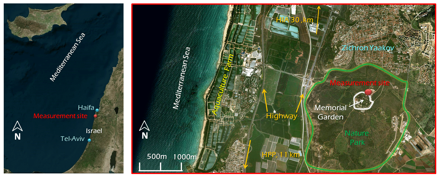
Figure 1Satellite images of the measurement site at Ramat Hanadiv Nature Park. Left: location of the measurement site (red dot). Right: zoomed in image of the surrounding area of the measurement site (red dot). Background imagery from © Google Earth.
2.2 Field measurements
The field measurements were taken at the Ramat Hanadiv site from the summer until the late autumn of 2015 (6 July–12 October 2015). The set of instruments included a platform for eddy covariance measurements of BVOCs, O3, carbon dioxide (CO2) and water vapor (H2O), trace-gas mixing ratios including O3, NOX, SO2 and CO, and basic meteorological conditions using an air-conditioned mobile laboratory and two towers (Fig. S2). Note that due to technical problems, VOC fluxes were not evaluated. The sampling routine and schematic of the setup were described in Li et al. (2018) and are summarized in Fig. S2.
The measurement and analysis of VOC concentrations include the following. VOC measurements were conducted using a proton transfer reaction time-of-flight mass spectrometer (PTR-ToF-MS; PTR-ToF-MS 8000, Ionicon Analytik GmbH, Innsbruck, Austria). A detailed description of the instrument can be found in Graus et al. (2010) and Jordan et al. (2009).
The PTR-ToF-MS was placed inside an air-conditioned mobile laboratory, and ambient air was pulled at a rate of about 35 L min−1 through an external PFA Teflon tube (3∕8” outer diameter, OD, 5∕16” inner dimension, ID) and subsampled by the PTR-ToF-MS at a rate of 0.5 l min−1 via a 1∕16” OD (1 mm ID) polyetheretherketone (PEEK) tube. The instrument inlet and drift tube were heated to 80 ∘C, the drift pressure was set to 2.3 mbar, and the voltage was set to 600 V; all settings were maintained at constant levels throughout the measurements, corresponding to an E∕N ratio of 140 Td. Measured data were recorded by a computer at 10 Hz.
The PTR-ToF-MS was calibrated every 1–2 d for background (zero) and weekly for sensitivity (span), subject to technical limitations (see Table S1 in the Supplement). The background (zero) calibration was conducted by sampling ambient air which was passed through a catalytic converter heated to 350 ∘C. The sensitivity calibration was performed using gas standards (Ionicon Analytik GmbH, Austria) containing methanol (0.99±8 % ppmv), acetonitrile (0.99±6 % ppmv), acetaldehyde (0.95±5 % (ppmv), ethanol (1.00±5 % ppmv), acrolein (1.01±5 % ppmv), acetone (0.98±5 % ppmv), isoprene (0.95±5 % ppmv), crotonaldehyde (1.01±5 % ppmv), 2-butanone (0.99±5 % ppmv), benzene (0.99±5 % ppmv), toluene (0.99±5 % ppmv), o-xylene (1.02±6 % ppmv), chlorobenzene (1.01±5 % ppmv), α-pinene (1.01±5 % ppmv) and 1,2-dichlorobenzene (1.02±5 % ppmv) to obtain gas mixtures ranging from 1 to 10 ppbv. Mixing ratios of compounds for which no gas standard was available were calculated using default reaction rate constants (see Sect. S1). The PTR-ToF-MS raw hdf5 (h5) files were preprocessed by a set of routines included in the PTRwid processing suite within an Interactive Data Language (IDL) environment and described in detail in Holzinger (2015). Further data processing was performed by customized multistep MATLAB (Mathworks Inc.) postprocessing routines, which included the processing of calibration, ambient measurements, chemical formula assignment, and comprehensive quality control similar to Tang et al. (2016). The list of compounds inferred from chemical formulas and further analysis (e.g., correlation matrix, diel variability and fragmentation patterns) is shown in Table S2. The uncertainties are listed according to whether a compound was explicitly calibrated and an accurate proton reaction rate constant was used (Sect. S1; Cappellin et al., 2012; Yuan et al., 2017) or a default reaction rate constant ( cm s−1) for unidentified ions was employed (not reported here).
Measurements of other trace gases and micrometeorology include the following. Complementary measurements included the quantification of mixing ratios of carbon monoxide (CO), sulfur dioxide (SO2), nitrogen oxides () and ozone (O3) using models 48i, 43s, 42i and 49i, respectively (Thermo Environmental Instruments Inc., Waltham, MA, USA), with manufacturer-reported limits of detection of 4.0 ppm and 0.1, 0.4 and 1.0 ppbv, respectively. These monitors were periodically calibrated to avoid drift in their accuracy. Trace-gas mixing ratios were recorded by a CR1000 data logger (Campbell Scientific, Logan, UT, USA) at a frequency of 1 min. Wind speed and wind direction were measured using an R.M. Young wind monitor 05103 (R.M. Young, Traverse City, MI, USA), the air temperature and relative humidity with a CS500 probe (Campbell Scientific), and the global radiation with a Kipp and Zonen CM3 pyranometer (Kipp and Zonen, Delft, Netherlands). These measured data were recorded with a CR10X data logger (Campbell Scientific) at a 10 min frequency. Overall, the measurements resulted in 20 d of high-quality, complete data which were divided into six different periods due to instrument downtime (see Sect. S1).
2.3 Model simulations of BVOC emission
The Model of Emissions of Gases and Aerosols from Nature version 2.1 (MEGAN v2.1; Guenther et al., 2012) was applied to estimate the emission flux of BVOCs from the nature park according to the vegetation type, as well as the on-site measured solar radiation, temperature, soil moisture, vegetation-cover fraction and leaf area index, using the following general formula to estimate the emission flux of species i (Fi):
where εi, j is the emission factor (representing the emission under standard conditions) of vegetation type j, γi is the emission activity factor which reflects the impact of environmental factors and phenology, and χj represents the vegetation effective fractional coverage area. The landscape average emission factor was estimated using the observed plant species composition at the field site (see Sect. 2.1). The major driving variables of the model are solar radiation, calculated leaf temperature, leaf age, soil moisture and leaf area index. The actual measured parameters at Ramat Hanadiv were used as input for the model, including vegetation and soil type, vegetation coverage fraction and leaf area index, soil water content, and meteorological data measured in situ. Note that only the nature park was simulated by MEGAN v2.1, while potential emissions from a nearby, relatively small memorial garden were not taken into account.
3.1 Seasonal and diel trends in measured BVOCs
Figure 2 presents the daytime average mixing ratios for selected VOCs measured in the field along with the corresponding daytime average temperatures. The presented data are not continuous due to instrument unavailability and were, therefore, separated into seven different measurement periods during the year 2015, as shown in Table 1.
Table 1Measurement periods and corresponding daytime mean of meteorological parameters used for the analyses* including temperature (T), photosynthetically active radiation (PAR), relative humidity (RH), wind direction (WDD) and wind speed (WDS).
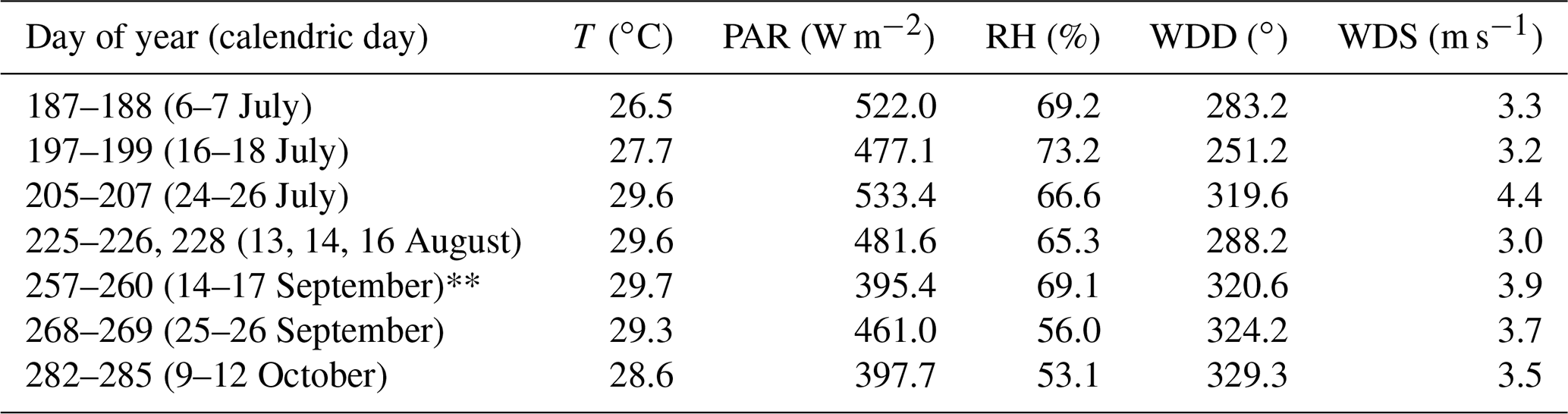
* See Table S1 for data availability and exclusion. Discussed only in relation to Fig. 2 considering irregular meteorological conditions (see Sect. S6).
Figure 2 presents both VOCs dominated by biogenic sources (BVOCs) and VOCs dominated by anthropogenic emission sources, although no compound can be regarded as exclusively biogenic or anthropogenic. The former include MTs (, , ), isoprene + 2-methyl-3-buten-2-ol (MBO) (; m69), DMS (), acetone (), acetaldehyde () and the sum of methyl vinyl ketone and methacrolein (MVK + MACR; ) (Janson and de Serves, 2001; Kanda et al., 1995; Karl et al., 2003; Park et al., 2013b). The latter include 1,3-butadiene () (Knighton et., 2009) and hydrogen sulfide (H2SH+; ) (Li et al., 2014). It is interesting to note that both MVK and MACR can have an anthropogenic source and be an oxidation product of isoprene (Fares et al., 2015; Jardine et al., 2013). Furthermore, this signal may receive contributions from dihydrofurans.
The dominating source behavior for BVOCs is reflected in their diurnal cycle, which was characterized by an increase in their mixing ratios from morning to around noontime or afternoon, followed by a gradual decrease until sunset (see Figs. S3–S9). We found similar day-to-day trends in the mixing ratios of all BVOCs, particularly of acetone, acetaldehyde and the MTs. This strongly reinforces the predominantly biogenic origin for these four species, considering that MTs are expected to be primarily emitted from biogenic sources in the studied area in the absence of any nearby wood industry. H2S and butadiene show significantly different trends in the mixing ratios, suggesting a dominating anthropogenic contribution for these species with a potential contribution from microbial activity (Misztal et al., 2018).
Overall, the day-to-day trend in the BVOC mixing ratios appears to follow the temperature but exhibits only a relatively weak correlation with daily temperature variation (Fig. 2). DMS showed the strongest correlation with the average daytime temperature (r2=0.27; see Sect. 3.2.2), corresponding to a significant increase in the mixing ratios between early summer (0.072±0.005 ppb, day of year, DOY, 188) and the end of summer (0.19±0.040 ppb, DOY 254), which decreased during the autumn (0.17±0.015 ppb, DOY 255, to 0.066±0.011 ppb, DOY 283). The other BVOCs, except for isoprene + MBO, showed a gradual increase in their average mixing ratios during the summer and early autumn (DOY 198–269; acetone from 3.74±0.767 ppbv to 4.33±0.471 ppbv, acetaldehyde from 1.64±0.595 ppbv to 3.09±0.496 ppbv, MT from 0.089±0.021 ppbv to 0.237±0.120 ppbv and MVK + MACR from 0.125±0.048 ppbv to 0.252±0.070 ppbv) and lower average mixing ratios in the autumn and early winter (DOY 270–286; DMS 0.091±0.026 ppbv, acetone 3.96±1.04 ppbv, acetaldehyde 1.86±0.97 ppbv, MT 0.139±0.064 ppbv, isoprene + MBO 0.182±0.093 ppbv and MVK + MACR 0.153±0.098 ppbv), which can be explained by the correlation with air temperature (Fig. 2). During DOY 257–260, BVOCs showed elevated mixing ratios (daytime averages for DMS, acetone, acetaldehyde, H2S, MT, isoprene + MBO and MVK + MACR were 0.122±0.016 ppbv, 13.6±3.26 ppbv, 8140±1.18 ppbv, 0.046±0.021 ppbv, 1.97±0.215 ppbv, 7.68±0.218 ppbv and 0.644±0.084 ppbv, respectively), as well as irregular diurnal shape, which may be attributed to synoptic-scale-induced processes (see Sect. S6). We, therefore, did not use these measurements for further analyses.
The diurnal profile of isoprene + MBO suggests a predominantly biogenic source due to a clear daytime increase and a correlation with temperature for most of the periods (Figs. 4 and S3–S9). However, its day-to-day mixing ratios showed higher variability (Fig. 2), which was quite different from both DMS and the other BVOCs. The origin of the BVOCs is explored in the next section.
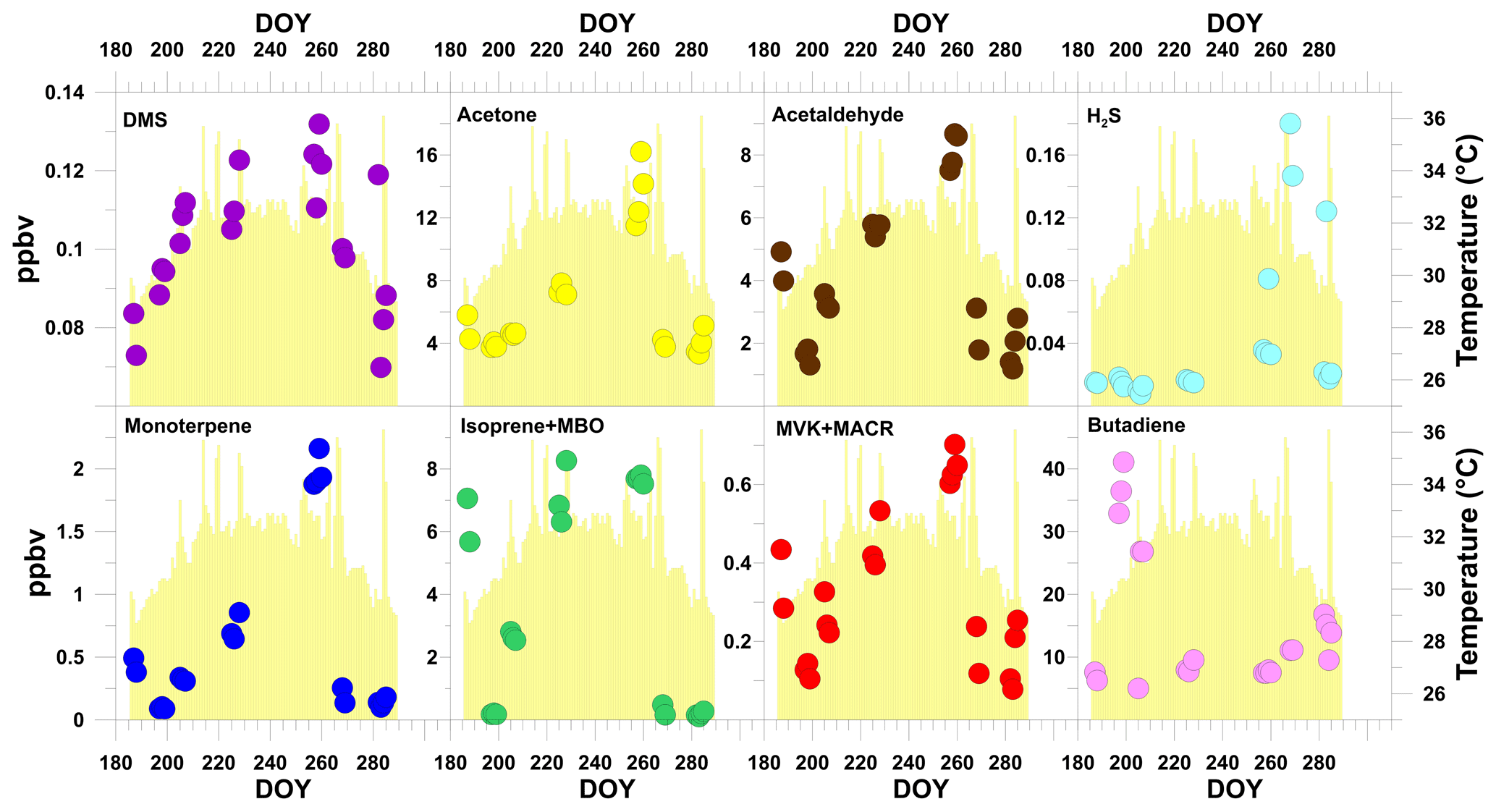
Figure 2The daytime average of selected VOCs. Yellow bars indicate the average daily temperature. DOY indicates the day of the year. For average diurnal profiles, see Figs. S3–S9.
3.2 Origin of the BVOCs
To explore the potential sources of the BVOCs, we calculated for each wind sector the percentage of time corresponding to several mixing ratio ranges individually for each species (Fig. 3). Our findings indicate elevated mixing ratios for westerly and southeasterly wind components. The relatively elevated mixing ratios from the southeast can be attributed to emissions from the memorial garden, where frequent thinning of the vegetation can contribute to the generally elevated mixing ratios of plant-wounding BVOCs which may include acetaldehyde, MVK, MACR, acetone, MT (e.g., Brilli et al., 2011, 2012; Goldstein et al., 2004; Ormeño et al., 2011; Portillo-Estrada et al., 2015) and possibly isoprene (e.g., Kanagendran et al., 2018). While methanol, hexanal and hexenal measurements also indicated elevated mixing ratios from the southeast, our analysis did not clearly indicate a higher excess of these green-leaved species from the southeast compared to the other wounding BVOCs (Sect. S7). The elevated mixing ratios from the west may point to an additional contribution of marine origin, such as the Mediterranean Sea and/or the aquaculture farms, considering that the measurement site is surrounded by nearly homogeneous vegetation in all directions except for the memorial garden (Fig. 1). We found a smaller relative contribution of DMS from the southeast compared to the other BVOCs. The MEGAN v2.1 simulations indicated that the known plant species in the nature park should not be a significant source of isoprene. It is possible that other local plants, such as invasive species, contributed to the observed isoprene concentration, but this would require a large area covered by high-isoprene-emitting species to result in the observed isoprene concentration at this site.
The relatively strong contribution of isoprene + MBO from the southeast can be attributed to MBO emissions from conifer trees (Gray et al., 2003) in the memorial garden. Similar trends in the day-to-day variation in MVK + MACR, isoprene oxidation products and isoprene + MBO (Fig. 2) could imply the contribution of the memorial garden to isoprene emissions. However, kinetic analysis indicated that the isoprene emissions from the memorial garden are much too small to account for the observed MVK + MACR associated with transported air masses from the memorial garden (see Sect. S4). The elevated mixing ratios of isoprene + MBO from the west may be primarily attributed to the emission of isoprene from marine organisms, as discussed in Sect. 3.2.1. The origin of DMS is further addressed in Sect. 3.2.2.
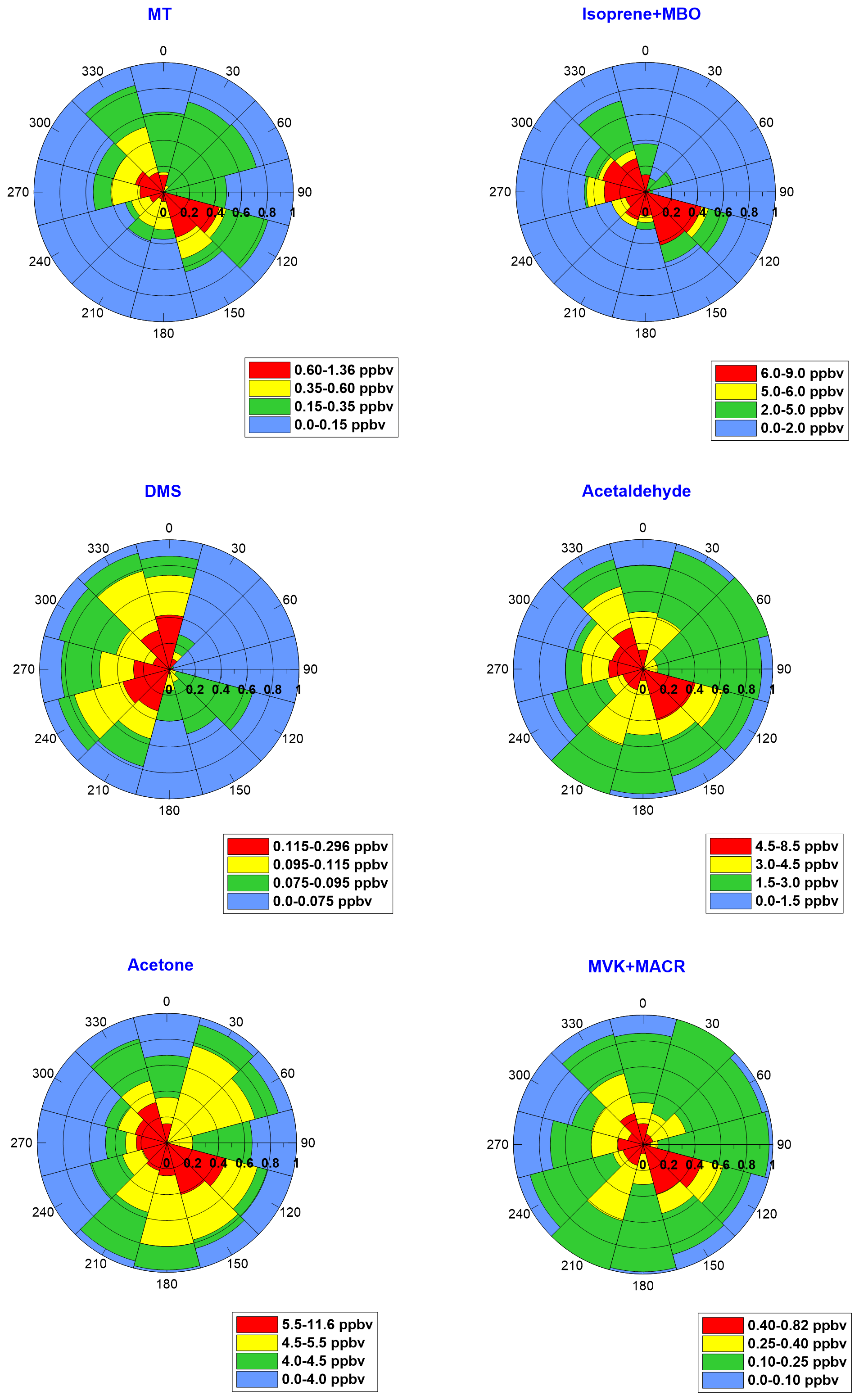
Figure 3BVOC mixing ratios as a function of the contribution from each wind sector during the daytime. The radial dimension represents the fraction of time for each wind sector during which the mixing ratios were within a certain range, as specified in the color key.
3.2.1 Origin apportionment of measured isoprene + MBO
For potential anthropogenic emission sources of isoprene + MBO, the indication from the MEGAN v2.1 simulations that the known plant species in the nature park are not a significant source of isoprene may suggest a significant contribution of the measured isoprene from anthropogenic sources. Moreover, as demonstrated in Sect. 3.1, the isoprene + MBO day-to-day variations differed from those of most of the other BVOCs with remarkably high variations in its mixing ratios ranging from 0.03 ppbv to nearly 9 ppbv (Fig. 2; Table S3). These day-to-day variations apparently masked the seasonal correlation of isoprene with temperature (see Fig. S10). Two highways to the west (Fig. 1) are the major potential anthropogenic isoprene emission sources at the site. The low correlation between the diurnal profile of isoprene and those of acetonitrile, benzene, toluene and carbon monoxide (see Figs. S12–S17 and S19) strongly supports the theory that there is no significant contribution to isoprene mixing ratios from traffic on the two highways, considering that benzene, toluene and carbon monoxide can be used as indicators for emissions from transportation. The dominant contribution of biogenic over anthropogenic sources to isoprene is further discussed in the following.
For potential biogenic emission sources of isoprene + MBO, Fig. 4 presents a scatter plot of isoprene + MBO mixing ratios vs. temperature T for the six measurement periods. For the two periods with high and low isoprene + MBO mixing ratios, there was a clear typical biogenic diurnal trend with a maximum around noontime. This finding reinforces the notion that isoprene + MBO originates predominantly from biogenic sources. We did not, however, observe a positive correlation between isoprene + MBO mixing ratios and air T in all six periods (Table 1). Furthermore, in most cases, we found no exponential increase in isoprene + MBO with air T, as is expected in the case of a nearby local biogenic source (e.g., Bouvier-Brown et al., 2009; Fares et al., 2009, 2010, 2012; Goldstein et al., 2004; Guenther et al., 1993; Kurpius and Goldstein, 2003; Richards et al., 2013). This might be related to the fact that the m69 signal is affected by the mixing ratios of both isoprene and MBO emitted locally and further away, while the local air temperature did not reflect changes of more distant leaf temperatures or SSTs. Therefore, we partitioned the isoprene + MBO signal.
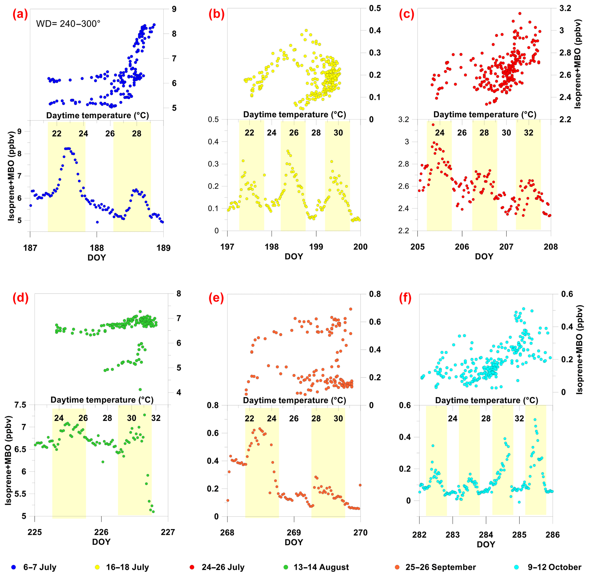
Figure 4Isoprene + MBO (m69) diurnal average mixing ratios and time series. (a–f) Regression scatter of measured MBO + isoprene (ISP + MBO) vs. temperature (a, b, c) and the time series of isoprene + MBO (d, e, f) for the six measurement periods: DOY 187–188 (a), DOY 197–199 (b), DOY 205–207 (c), DOY 225–226 (d), DOY 268–269 (e), DOY 282–285 (f). The scatter of the measured MBO + isoprene vs. temperature (a, b, c) excludes measurements associated with wind direction from the memorial garden (90–150∘).
For the partitioning of isoprene + MBO signal, we used the fact that MBO can also be detected at (m87), which typically accounts for 13 %–25 % of the total MBO signal (Kaser et al., 2013; Park et al., 2012, 2013a, 2013b), to learn about the ratio between the isoprene and MBO mixing ratios. Note that other species in addition to MBO, including methyl propyl ketone, pentanal and other C5H10O compounds, may contribute to the m87 signal. Hence, we refer in the following to m87 as MBO* to reflect this fact. Figure 5a presents the mixing ratios for m69 vs. m87 ∕ m69. Periods with high mixing ratios for m69 were associated with a very low m87 ∕ m69 ratio (less than 2 %), which suggests that the emissions are predominantly of isoprene. Figure 5a also indicates that m87 ∕ m69 >25 % was mostly measured during the nighttime, twilight and early morning. For low m69, the ratio matches the typical MBO ratio, m87 ∕ m69, which ranges between 13 % and 25 % or higher (Fig. 5a).
For the isoprene origin, Fig. 6 further presents the diurnal profile for m87 ∕ m69 <13 %, as well as the corresponding mixing ratios vs. temperature, separately for each measurement day. Interestingly, some of the measurement days presented in Fig. 4 were associated with no m87 ∕ m69 <13 %, which is why there are fewer measurement days in Fig. 6 than in Fig. 4. The diurnal profiles in Fig. 6 support a biogenic origin for isoprene, although they were more scattered for 25–27 July. Figure 6 also demonstrates the positive correlation between the isoprene mixing ratio and temperature during all measurement days, while on several days, a sharp increase in isoprene with temperature occurred for T>∼ 26–28 ∘C (e.g., 6, 7 July and 16 August). In general, a higher correlation with temperature was obtained for m87 ∕ m69 <13 % (Fig. 6) than for all m69 signals (i.e., Fig. 6 vs. Fig. 4), reinforcing the biogenic origin of isoprene with a relatively strong dependency on temperature. Furthermore, regression of m87 ∕ m69 >13 % with temperature does not indicate a clear dependency of mixing ratios on temperature, suggesting different emission controls for MBO* and isoprene (see Fig. S21). While the MBO* mixing ratios tended to be controlled by both temperature and solar radiation, isoprene was predominantly governed by the former, which is in agreement with a previous study (see Kaser et al., 2013).
To study the origin of isoprene, we analyzed the fraction of time for which m87 ∕ m69 < 13 % vs. wind direction (Fig. 5b). We found that m87 ∕ m69 < 13 % predominantly corresponds to a western origin. These results suggest a significant contribution of isoprene from the sea or the aquaculture farm located to the west of the measurement site (Fig. 1), considering that the measurement site is nearly homogeneously surrounded by mixed Mediterranean vegetation except for the memorial garden to the southeast. Furthermore, MEGAN v2.1 simulations predicted a negligible emission rate for isoprene from the nature park. In addition, the relatively high day-to-day variation in isoprene mixing ratios (Fig. 6) further support emissions induced by marine organisms.
In some cases (∼4 % of the time), elevated m87 ∕ m69 <13 % was also recorded from the southwest and northwest, which according to simulations by the Hybrid Single Particle Lagrangian Integrated Trajectory (HYSPLIT) model can be entirely attributed to transport from either the sea or the aquaculture farms (see Fig. S20). The relatively small fraction of time during which m87 ∕ m69 <13 % was from the southeast can be attributed to the emission of isoprene, while most of the elevated isoprene + MBO from this direction (Fig. 3) can be attributed to MBO from conifers.
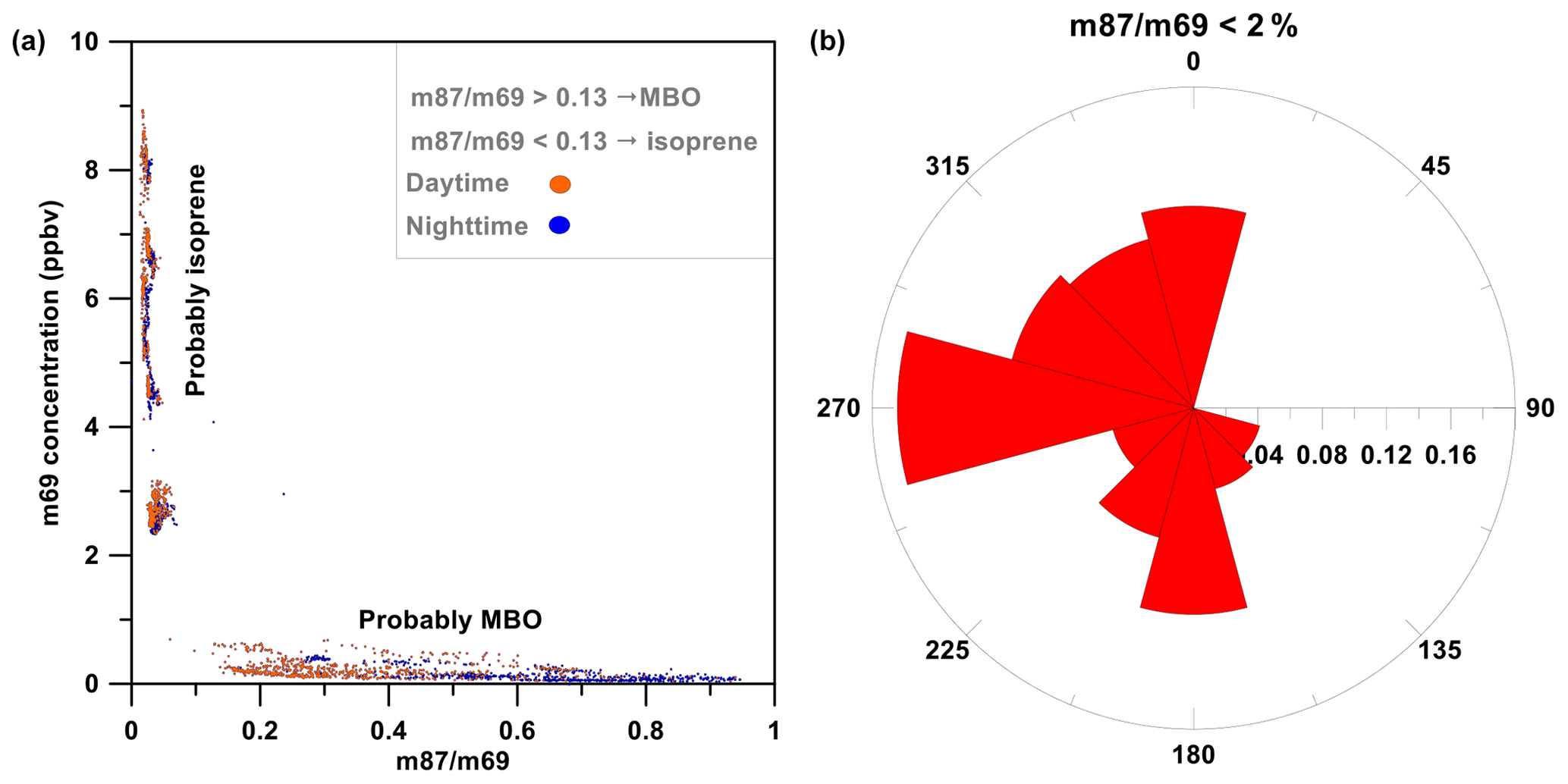
Figure 5Isoprene and MBO* origins. (a) Scatter plot of m69 mixing ratios as a function of the m87 ∕ m69 ratio. Low and high ratios indicate a predominant contribution of MBO* (see definition in Sect. 3.2.1) and isoprene, respectively. The orange dots were measured during the daytime and the dark blue dots during the night. (b) Fraction of time for each wind sector for which m87 ∕ m69 was less than 13 %.
Two facts support isoprene's predominant sea origin rather than the aquaculture farms. First, back trajectories using HYSPLIT show no lower mixing ratios for m87 ∕ m69 <2 % and also in cases when the air masses were transported from the sea but not over the aquaculture farms compared to transport of air masses over the aquaculture (e.g., Figs. 4 and S20). Second, marine organisms have relatively short life cycles, typically a few days (Tyrrell, 2001), and would likely have a variable source strength from the aquaculture farms, which would not coincide with the similar measured m87 ∕ m69 <2 % mixing ratios for different wind directions during a specific day. Our measurements indicated no dependence of high m87 ∕ m69 <2 % mixing ratios on wind direction during the day, reinforcing the sea's dominant role in isoprene emission rather than the aquaculture farms. Yet, while it is likely that the Mediterranean Sea is the dominant isoprene source rather than the aquaculture farms or the nature park, additional measurements on the coastline are required to quantify the contribution of other isoprene sources.
Interestingly, the isoprene mixing ratios during the nighttime remained relatively high (∼ 5–6 ppb) (Fig. 5a) possibly due to relatively small oxidative sink strength during the night. The daytime and nighttime isoprene lifetime can be estimated based on its reaction with OH, NO3 and O3. We estimated the average daytime OH and nighttime NO3 concentrations based on the Mediterranean Intensive Oxidant Study (MINOS) campaign in Finokalia, Crete (Berresheim et al., 2003; Vrekoussis et al., 2004), at (Berresheim et al., 2003) and (Vrekoussis et al., 2004), respectively. Using these concentrations, the reported rate constants for isoprene with OH and NO3 of (Stevens et al., 1999) and (Winer et al., 1984), respectively, and measured O3 levels, we obtained daytime and nighttime isoprene lifetimes of ∼37 min and ∼3.8 h, respectively. Considering the relatively moderate decrease in the measured isoprene during the night (Figs. S12–S17), this result indicates stronger isoprene emissions during the daytime but does not rule out nighttime isoprene emissions.
A rough estimation of the isoprene production rate can be calculated by subtracting the isoprene loss rate, evaluated from its calculated lifetime, from its measured mixing ratios. These simplified calculations indicate a daytime and nighttime isoprene production rate ranging between and ppbv s−1 (average ppbv s−1) and between and ppbv s−1 (average ppbv s−1), supporting a much smaller isoprene production rate during the night vs. daytime.
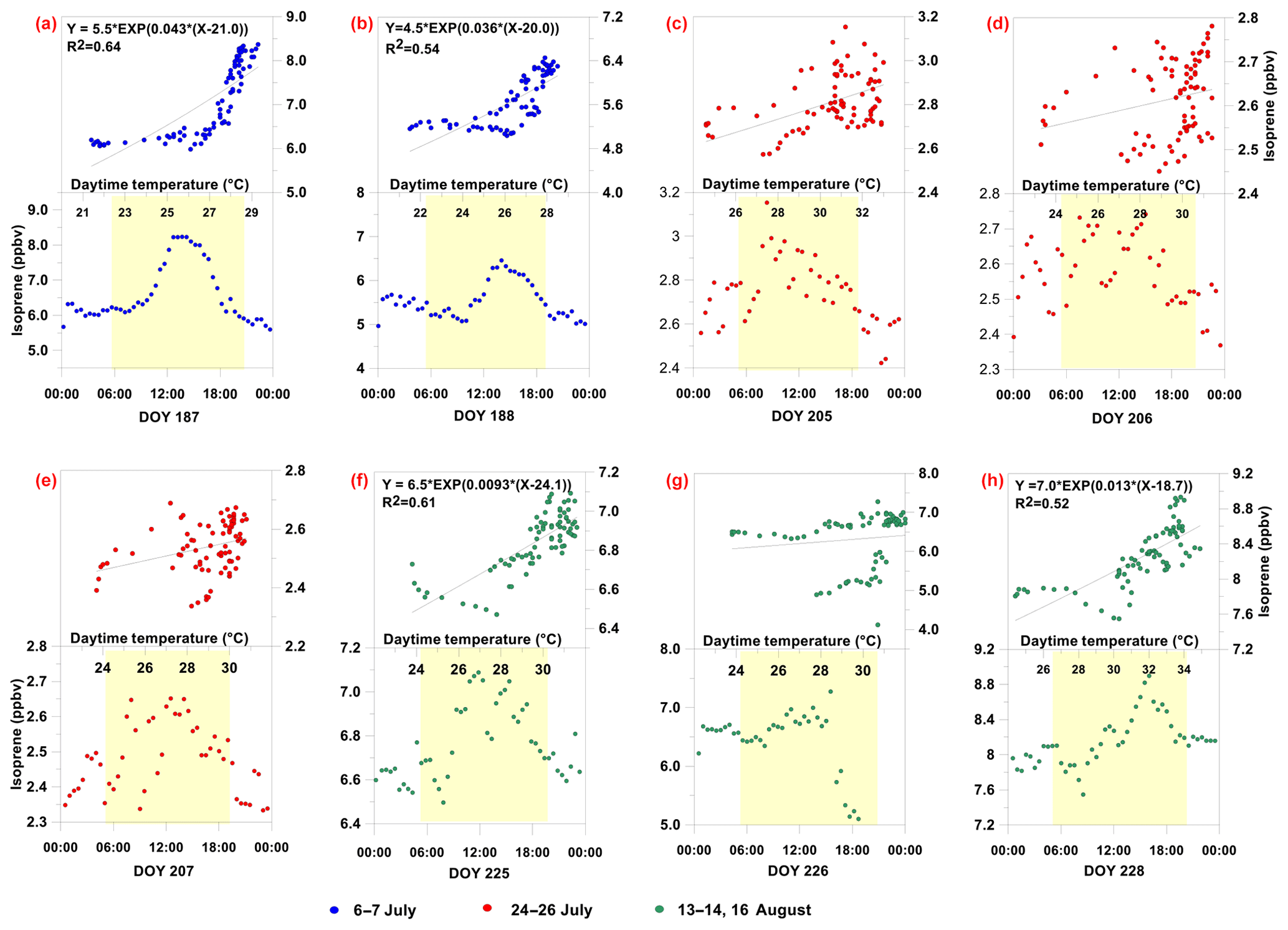
Figure 6Isoprene (m87 ∕ m69 <13 %) diurnal average mixing ratio and dependence on temperature. Upper panels show scatter plots between measured m87 ∕ m96 <13 % and temperature, as well as the corresponding regression equation and nonlinear exponential coefficient (R2) in cases when R2>0.50. Lower panels present that of m87 ∕ m96 <13 %. Yellow shaded areas represent daylight hours.
3.2.2 Origin and characterization of DMS emission
The discussion in Sect. 3.1 suggests that DMS is primarily emitted from the west, pointing to a dominant marine emission source with the less elevated mixing ratios probably associated with emissions from vegetation. According to the MEGAN v2.1 simulation, the nature park's vegetation is a potent source of DMS (average flux equals 0.477 mg m−2 h−1, which is slightly higher than the flux measured from insolated branches; Jardine et al., 2015; Yonemura et al., 2005), while our analysis points to stronger emissions from the memorial garden (see Fig. 3). As with isoprene, the insensitivity of DMS mixing ratios to wind direction for westerly winds rules out a significant contribution of the aquaculture farms to the measured DMS. This suggests that the sea is a major source for DMS with an apparently strong dependency on temperature (Figs. 2, 3). DMS showed much less day-to-day variations in its mixing ratios compared to isoprene and other BVOCs. This corresponded to a clear day-to-day correlation of DMS mixing ratios with air temperature (Fig. 2). Figure 7 demonstrates a clear increase in the mixing ratios with air temperature throughout the measurement period. Note that no significant dependency of DMS on global solar radiation was observed.
The DMS mixing ratios peaked at ∼0.18 ppbv. This figure is about an order of magnitude lower than at the ocean surface (Tanimoto et al., 2014), about an order of magnitude lower than in the Southern Ocean (Koga et al., 2014), slightly lower than the maximum concentrations in the southern Indian Ocean (Boucher et al., 2003) and similar to the maximum concentrations on the coasts of Tasmania (Boucher et al., 2003). Interestingly, the mixing ratios measured in this study are lower by about 1–2 orders of magnitude than those measured in the same region during August 1995 (Ganor et al., 2000). This could be attributed to a change in the marine biota as a consequence of seawater warming considering that reported SST during mid-August 2015 (IOLR, 2015) was higher than the SST reported by Ganor et al. (2000) by up to 1.5–2.1 ∘C.
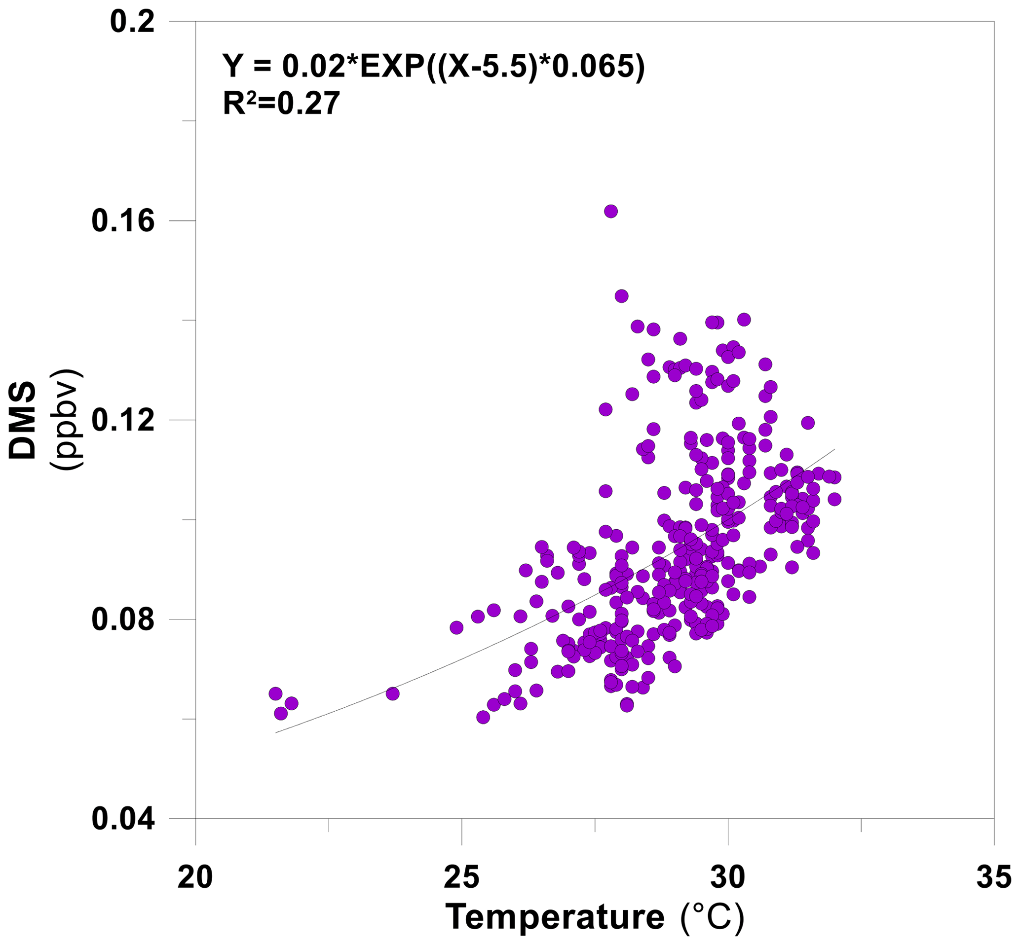
Figure 7Daytime DMS mixing ratios from the western sector (marine source) as a function of the temperature along the measurement campaign. An exponential fit between the two is included.
3.2.3 Origin and characterization of other BVOCs
Our findings in Fig. 2 strongly suggest a common source for other BVOCs with isoprene. We could not, however, use a wind-direction-based analysis to indicate BVOCs' origin from the sea since both sea and vegetation are located to the west of the measurement point (see Fig. 1), and in contrast to isoprene, the other BVOCs were indicated by MEGAN v2.1 to be locally emitted. Furthermore, those BVOCs were less variable with wind direction than isoprene was. We used MT summer measurements from two other sites in Israel to assess whether MTs are likely to be transported to the measurement site.
We used the ratio between MT flux and mixing ratio at three sites as a basis to address this inquiry. Note that according to the MEGAN v2.1 simulations (see Sect. 2.3), the MT emissions in Ramat Hanadiv were driven by Quercus calliprinos (48.1 %), Pistacia lentiscus (19.8 %), Phillyrea latifolia (7.12 %) and Cupressus spp. (6.17 %), as well as other species (see Sect. S5), in contrast to the two Pinus halepensis plantations, Birya and Yatir. While the fact that MT is not emitted by the same vegetation species should not significantly affect our analysis, we recognize that there may be differences in the MT composition and atmospheric oxidation capacity at the three sites which would influence MT lifetimes and lead to some differences in the flux-to-concentration ratios. According to MEGAN v2.1, the average and maximal daytime MT fluxes were 59 and 152 µg m−2 h−1, respectively. While this predicted average flux is lower than the mean MT measurements in the Birya and Yatir forests (∼200 and , respectively; Seco et al., 2017), the corresponding measured mixing ratios in our study are generally higher than those measured in those two sites, where the MT mixing ratios reached above 0.5 ppbv for Birya in only a few cases and the maximum was 0.2 ppbv in Yatir. Note that the higher mixing ratios in our study, as compared to these two sites, were associated with wind direction either from the memorial garden or from the western sector (Fig. 3). This supports a relatively small local contribution of MTs in our study compared to seawater.
3.3 Concentrations of isoprene and DMS originating from the Levantine Basin
Previous studies demonstrated the trade-off between DMS and isoprene in the marine boundary layer due to species distribution and climate, suggesting that most regions are a source of either isoprene or DMS but not both. While isoprene is emitted from species that are more abundant in warmer regions and low-to-middle latitudes, DMS is predominantly emitted in colder regions and higher latitudes (Dani and Loreto, 2017). This is in agreement with the relatively high isoprene ∕ DMS mixing ratios in our study. The SST in the Levantine Basin is relatively high, exceeding 30 ∘C in August 2015 at a distance of 2 km from the coastline (IOLR, 2015). Further, SST plays a significant role in determining which phytoplankton will dominate, and, for a given marine organisms population, higher temperature and solar radiation tend to enhance their BVOC emissions, including DMS and isoprene (Dani and Loreto, 2017). The strong emission of isoprene from the Levantine Basin can be attributed primarily to its relatively high SST, considering the well-known correlation of isoprene emission with SST (Dani and Loreto, 2017; Exton et al., 2013).
The relatively warm and oligotrophic sea enables cyanobacteria to become a large fraction of marine primary production and phytoplankton (Krom et al., 2010; Paerl and Otten, 2013; Pedrotti et al., 2017; Sarma, 2013) in the Levantine Basin, which favors, in turn, the emission of isoprene over other BVOCs, including DMS. Previous measurements have indicated the presence of cyanobacteria in the Levantine Basin during the summer of 2015 (Herut et al., 2016), with the cyanobacteria Synechococcus and Prochlorococcus being the most abundant phytoplankton along the coasts of Israel during August 2015. A laboratory experiment demonstrated the emission of isoprene from the latter (Shaw et al., 2003). Other micro-organisms in the Levantine Basin (mostly dinoflagellates and diatoms) are generally less abundant. Thalassiosira pseudonana diatoms are also abundant along the coasts of Israel, which raises the possibility that the emission of isoprene from the sea is also influenced by this species. A laboratory experiment using proton transfer reaction mass spectrometry indicated the emission of isoprene, as well as methanol, acetone and acetaldehyde from Thalassiosira pseudonana diatoms, but isoprene is the only one among these that is not consumed by bacterioplankton within the water column (Halsey et al., 2017).
DMS can be also emitted by diatoms but at lower rates under warmer conditions (Dani and Loreto, 2017; Levasseur et al., 1994). In addition, DMS is a common microbial VOC formed in various marine environments by the bacterial decomposition of dimethylsulfoniopropionate (DMSP) (Bourne et al., 2013; Howard et al., 2008). DMS in the marine boundary layer is mostly emitted by dinoflagellates and haptophyte coccolithophores. Dinoflagellates, as well as Thalassiosira pseudonana diatoms, were constantly observed along the coast in estuary zones several kilometers from the measurement site (Herut et al., 2016). This might explain the relatively minor day-to-day variations in the mixing ratios of DMS (Fig. 2) which in turn resulted in a relatively high correlation of the mixing ratios with T throughout the measurement periods. Cyanobacteria blooms and collapses depend on the nutrient supply and have no seasonality (Paerl and Otten, 2013), which can be an additional reason for the fluctuations in isoprene.
Our findings indicate that high isoprene emissions from the Eastern Mediterranean Sea contribute up to ∼9 ppb several kilometers inland from the sea shore. The apparently strong emission of isoprene can be attributed primarily to the relatively high SST of the Levantine Basin, considering the well-known correlation of isoprene emissions with SST growth conditions (Dani and Loreto, 2017; Exton et al., 2013). Furthermore, isoprene mixing ratios tended to strongly increase with diurnal increases in air temperature, but there was no correlation with solar radiation. Our analysis points to cyanobacteria as a dominant source for the isoprene emissions, as well as other possible marine microbiomes, supporting previous findings (Arnold et al., 2009; Bonsang et al., 2010; Dani and Loreto, 2017; Hackenberg et al., 2017; Shaw et al., 2003). Measured DMS mixing ratios were lower by 1–2 orders of magnitude than those measured in 1995 (Ganor et al., 2000) in the same area during the same season, suggesting a strong impact of SST on the decadal change in DMS emissions via changes in species composition. Considering that, according to the IPCC, ocean SST is expected to rise by 5 ∘C by the year 2100 (Hoegh-Guldberg et al., 2014), efforts are required to adequately represent the complex dependency of marine BVOC emissions, such as isoprene and DMS, on SST, to improve the predictability of both air quality and climate models. Our study results indicate that this increase in SST can significantly increase the emission of isoprene into the MBL. This can greatly affect air quality, considering its high photochemical reactivity, with particularly negative implications in urbanized coastal areas where onshore wind typically occurs during the daytime and is controlled by the sea to land breeze. Furthermore, elevated isoprene emissions are expected from coastal areas where coastal upwelling can significantly affect biological activity, which was shown to correlate with BVOC emissions (Gantt et al., 2010).
A comprehensive evaluation of the impact of marine organism emissions on both the atmospheric chemistry and radiative budget should rely on a suite of gases. Along with the high isoprene levels, relatively low DMS mixing ratios were observed under the studied conditions, which supports previous studies that have indicated a general contrasting spatial distribution partially controlled by SST and latitude (Yokouchi et al., 1999) and lower DMS emission under relatively low temperature (Dani and Loreto, 2017). While DMS and isoprene emissions are influenced in a contrasting manner by changes in SST, both tend to rise in response to a SST increase for a given phytoplankton population (Dani and Loreto, 2017), as supported by this study.
A significant contribution of oceanic emissions of other BVOCs, such as acetone, acetaldehyde and monoterpenes, has also been reported by previous studies. We found supporting indications for dominant emissions of MT from the Levantine Basin, further suggesting significant emissions of other BVOCs from this source. The analyses also indicate that estuaries play a potentially important role in facilitating the emission of DMS, and probably additional BVOCs, by maintaining a suitable environment for phytoplankton growth. In agreement with a previous study (Goldstein et al., 2004), our analyses suggest that thinning may play an important role in facilitating BVOC emissions, a mechanism which should be taken into consideration especially in urban areas with cultivated parks and gardens.
This study demonstrates that most of the VOCs studied here are controlled by both anthropogenic and marine and terrestrial biogenic emission sources, highlighting the need for the strict identification of the origin and representative models for both emission source types. Our study further highlights the Levantine Basin's capability to serve as a natural laboratory for studying both anthropogenic stress and climate change on marine BVOC emissions. More comprehensive research is required to directly address the impact of oligotrophication and increased SST on marine BVOC emissions.
Data are available upon request from the corresponding authors Eran Tas (eran.tas@mail.huji.ac.il) and Erick Fredj (erick.fredj@gmail.com).
The supplement related to this article is available online at: https://doi.org/10.5194/acp-20-12741-2020-supplement.
ET designed the experiments, MG and GL carried out the field measurements, and PKM and EF led the calibration, quality control and data processing. ABG set up the MEGAN v2.1 model. CD and ET led the analyses with contributions from all coauthors. ET and CD prepared the paper with contributions from all coauthors.
The authors declare that they have no conflict of interest.
We want to greatly thank the crew of Ramat Hanadiv and Gil Lerner for supporting the measurements. Eran Tas holds the Joseph H. and Belle R. Braun Senior Lectureship in Agriculture.
This research has been supported by the Israel Science Foundation (grant no. 1787/15).
This paper was edited by Andreas Hofzumahaus and reviewed by Silvano Fares and one anonymous referee.
Alvarez, L. A., Exton, D. A., Timmis, K. N., Suggett, D. J., and McGenity, T. J.: Characterization of marine isoprene-degrading communities, Environ. Microbiol., 11, 3280–3291, https://doi.org/10.1111/j.1462-2920.2009.02069.x, 2009.
Andreae, M. O.: Ocean-atmosphere interactions in the global biogeochemical sulfur cycle, Mar. Chem., 30, 1–29, https://doi.org/10.1016/0304-4203(90)90059-L, 1990.
Arneth, A., Monson, R. K., Schurgers, G., Niinemets, Ü., and Palmer, P. I.: Why are estimates of global terrestrial isoprene emissions so similar (and why is this not so for monoterpenes)?, Atmos. Chem. Phys., 8, 4605–4620, https://doi.org/10.5194/acp-8-4605-2008, 2008.
Arnold, S. R., Spracklen, D. V., Williams, J., Yassaa, N., Sciare, J., Bonsang, B., Gros, V., Peeken, I., Lewis, A. C., Alvain, S., and Moulin, C.: Evaluation of the global oceanic isoprene source and its impacts on marine organic carbon aerosol, Atmos. Chem. Phys., 9, 1253–1262, https://doi.org/10.5194/acp-9-1253-2009, 2009.
Ayers, G. P., Cainey, J. M., Gillett, R. W., and Ivey, J. P.: Atmospheric sulphur and cloud condensation nuclei in marine air in the Southern Hemisphere, Philos. Trans. R. Soc. B Biol. Sci., 352, 203–211, https://doi.org/10.1098/rstb.1997.0015, 1997.
Azov, Y.: Seasonal patterns of phytoplankton productivity and abundance in nearshore oligotrophic waters of the Levant Basin (Mediterranean), J. Plankton Res., 8, 41–53, https://doi.org/10.1093/plankt/8.1.41, 1986.
Beaugrand, G., Edwards, M., Brander, K., Luczak, C., and Ibanez, F.: Causes and projections of abrupt climate-driven ecosystem shifts in the North Atlantic, Ecol. Lett., 11, 1157–1168, https://doi.org/10.1111/j.1461-0248.2008.01218.x, 2008.
Beaugrand, G., Edwards, M., and Legendre, L.: Marine biodiversity, ecosystem functioning, and carbon cycles, P. Natl. Acad. Sci., 107, 10120–10124, https://doi.org/10.1073/pnas.0913855107, 2010.
Berresheim, H., Plass-Dülmer, C., Elste, T., Mihalopoulos, N., and Rohrer, F.: OH in the coastal boundary layer of Crete during MINOS: Measurements and relationship with ozone photolysis, Atmos. Chem. Phys., 3, 639–649, https://doi.org/10.5194/acp-3-639-2003, 2003.
Bijma, J., Pörtner, H. O., Yesson, C., and Rogers, A. D.: Climate change and the oceans – What does the future hold?, Mar. Pollut. Bull., 74, 495–505, https://doi.org/10.1016/j.marpolbul.2013.07.022, 2013.
Blando, J. D. and Turpin, B. J.: Secondary organic aerosol formation in cloud and fog droplets: A literature evaluation of plausibility, Atmos. Environ., 34, 1623–1632, https://doi.org/10.1016/S1352-2310(99)00392-1, 2000.
Bonsang, B., Polle, C., and Lambert, G.: Evidence for marine production of isoprene, Geophys. Res. Lett., 19, 1129–1132, https://doi.org/10.1029/92GL00083, 1992.
Bonsang, B., Gros, V., Peeken, I., Yassaa, N., Bluhm, K., Zoellner, E., Sarda-Esteve, R., and Williams, J.: Isoprene emission from phytoplankton monocultures: the relationship with chlorophyll-a, cell volume and carbon content, Environ. Chem., 7, 554, https://doi.org/10.1071/en09156, 2010.
Bopp, L., Resplandy, L., Orr, J. C., Doney, S. C., Dunne, J. P., Gehlen, M., Halloran, P., Heinze, C., Ilyina, T., Séférian, R., Tjiputra, J., and Vichi, M.: Multiple stressors of ocean ecosystems in the 21st century: projections with CMIP5 models, Biogeosciences, 10, 6225–6245, https://doi.org/10.5194/bg-10-6225-2013, 2013.
Boucher, O., Moulin, C., Belviso, S., Aumont, O., Bopp, L., Cosme, E., von Kuhlmann, R., Lawrence, M. G., Pham, M., Reddy, M. S., Sciare, J., and Venkataraman, C.: DMS atmospheric concentrations and sulphate aerosol indirect radiative forcing: a sensitivity study to the DMS source representation and oxidation, Atmos. Chem. Phys., 3, 49–65, https://doi.org/10.5194/acp-3-49-2003, 2003.
Bourne, D. G., Dennis, P. G., Uthicke, S., Soo, R. M., Tyson, G. W., and Webster, N.: Coral reef invertebrate microbiomes correlate with the presence of photosymbionts, ISME J., 7, 1452–1458, https://doi.org/10.1038/ismej.2012.172, 2013.
Bouvier-Brown, N. C., Goldstein, A. H., Gilman, J. B., Kuster, W. C., and de Gouw, J. A.: In-situ ambient quantification of monoterpenes, sesquiterpenes, and related oxygenated compounds during BEARPEX 2007: implications for gas- and particle-phase chemistry, Atmos. Chem. Phys., 9, 5505–5518, https://doi.org/10.5194/acp-9-5505-2009, 2009.
Boyce, D. G., Lewis, M. R., and Worm, B.: Global phytoplankton decline over the past century., Nature, 466, 591–6, https://doi.org/10.1038/nature09268, 2010.
Brilli, F., Ruuskanen, T. M., Schnitzhofer, R., Müller, M., Breitenlechner, M., Bittner, V., Wohlfahrt, G., Loreto, F., and Hansel, A.: Detection of plant volatiles after leaf wounding and darkening by proton transfer reaction “time-of-flight” mass spectrometry (ptr-tof), PLoS One, 6, 1–2, https://doi.org/10.1371/journal.pone.0020419, 2011.
Brilli, F., Hörtnagl, L., Bamberger, I., Schnitzhofer, R., Ruuskanen, T. M., Hansel, A., Loreto, F., and Wohlfahrt, G.: Qualitative and quantitative characterization of volatile organic compound emissions from cut grass, Environ. Sci. Technol., 46, 3859–3865, https://doi.org/10.1021/es204025y, 2012.
Broadgate, W. J., Malin, G., Küpper, F. C., Thompson, A., and Liss, P. S.: Isoprene and other non-methane hydrocarbons from seaweeds: A source of reactive hydrocarbons to the atmosphere, Mar. Chem., 88, 61–73, https://doi.org/10.1016/j.marchem.2004.03.002, 2004.
Calfapietra, C., Fares, S., Manes, F., Morani, A., Sgrigna, G., and Loreto, F.: Role of Biogenic Volatile Organic Compounds (BVOC) emitted by urban trees on ozone concentration in cities: A review, Environ. Pollut., 183, 71–80, https://doi.org/10.1016/j.envpol.2013.03.012, 2013.
Cappellin, L., Karl, T., Probst, M., Ismailova, O., Winkler, P. M., Soukoulis, C., Aprea, E., Märk, T. D., Gasperi, F., and Biasioli, F.: On quantitative determination of volatile organic compound concentrations using proton transfer reaction time-of-flight mass spectrometry, Environ. Sci. Technol., 46, 2283–2290, https://doi.org/10.1021/es203985t, 2012.
Carlton, A. G., Wiedinmyer, C., and Kroll, J. H.: A review of Secondary Organic Aerosol (SOA) formation from isoprene, Atmos. Chem. Phys., 9, 4987–5005, https://doi.org/10.5194/acp-9-4987-2009, 2009.
Carslaw, N., Jacobs, P. J., and Pilling, M. J.: Understanding radical chemistry in the marine boundary layer, Phys. Chem. Earth Pt. C, 25, 235–243, https://doi.org/10.1016/S1464-1917(00)00011-8, 2000.
Chiemchaisri, W., Visvanathan, C., and Jy, S. W.: Effects of trace volatile organic compounds on methane oxidation, Brazilian Arch. Biol. Technol., 44, 135–140, https://doi.org/10.1590/S1516-89132001000200005, 2001.
Curci, G., Beekmann, M., Vautard, R., Smiatek, G., Steinbrecher, R., and Theloke, J.: Modelling study of the impact of isoprene and terpene biogenic emissions on European ozone levels, Atmos. Environ., 43, 1444–1455, https://doi.org/10.1016/J.ATMOSENV.2008.02.070, 2009.
Dani, K. G. G. S. and Loreto, F.: Trade-Off Between Dimethyl Sulfide and Isoprene Emissions from Marine Phytoplankton, Trends Plant Sci., 22, 361–372, https://doi.org/10.1016/j.tplants.2017.01.006, 2017.
Debevec, C., Sauvage, S., Gros, V., Sciare, J., Pikridas, M., Stavroulas, I., Salameh, T., Leonardis, T., Gaudion, V., Depelchin, L., Fronval, I., Sarda-Esteve, R., Baisnée, D., Bonsang, B., Savvides, C., Vrekoussis, M., and Locoge, N.: Origin and variability in volatile organic compounds observed at an Eastern Mediterranean background site (Cyprus), Atmos. Chem. Phys., 17, 11355–11388, https://doi.org/10.5194/acp-17-11355-2017, 2017.
Derstroff, B., Hüser, I., Bourtsoukidis, E., Crowley, J. N., Fischer, H., Gromov, S., Harder, H., Janssen, R. H. H., Kesselmeier, J., Lelieveld, J., Mallik, C., Martinez, M., Novelli, A., Parchatka, U., Phillips, G. J., Sander, R., Sauvage, C., Schuladen, J., Stönner, C., Tomsche, L., and Williams, J.: Volatile organic compounds (VOCs) in photochemically aged air from the eastern and western Mediterranean, Atmos. Chem. Phys., 17, 9547–9566, https://doi.org/10.5194/acp-17-9547-2017, 2017.
Efrati, S., Lehahn, Y., Rahav, E., Kress, N., Herut, B., Gertman, I., Goldman, R., Ozer, T., Lazar, M., and Heifetz, E.: Intrusion of coastal waters into the pelagic eastern Mediterranean: in situ and satellite-based characterization, Biogeosciences, 10, 3349–3357, https://doi.org/10.5194/bg-10-3349-2013, 2013.
Exton, D. A., Suggett, D. J., McGenity, T. J., and Steinke, M.: Chlorophyll-normalized isoprene production in laboratory cultures of marine microalgae and implications for global models, Limnol. Oceanogr., 58, 1301–1311, https://doi.org/10.4319/lo.2013.58.4.1301, 2013.
Fares, S., Mereu, S., Scarascia Mugnozza, G., Vitale, M., Manes, F., Frattoni, M., Ciccioli, P., Gerosa, G., and Loreto, F.: The ACCENT-VOCBAS field campaign on biosphere-atmosphere interactions in a Mediterranean ecosystem of Castelporziano (Rome): site characteristics, climatic and meteorological conditions, and eco-physiology of vegetation, Biogeosciences, 6, 1043–1058, https://doi.org/10.5194/bg-6-1043-2009, 2009.
Fares, S., McKay, M., Holzinger, R., and Goldstein, A. H.: Ozone fluxes in a Pinus ponderosa ecosystem are dominated by non-stomatal processes: Evidence from long-term continuous measurements, Agric. For. Meteorol., 150, 420–431, https://doi.org/10.1016/j.agrformet.2010.01.007, 2010.
Fares, S., Weber, R., Park, J. H., Gentner, D., Karlik, J., and Goldstein, A. H.: Ozone deposition to an orange orchard: Partitioning between stomatal and non-stomatal sinks, Environ. Pollut., 169, 258–266, https://doi.org/10.1016/j.envpol.2012.01.030, 2012.
Fares, S., Paoletti, E., Loreto, F., and Brilli, F.: Bidirectional Flux of Methyl Vinyl Ketone and Methacrolein in Trees with Different Isoprenoid Emission under Realistic Ambient Concentrations, Environ. Sci. Technol., 49, 7735–7742, https://doi.org/10.1021/acs.est.5b00673, 2015.
Fogg, G. E.: Review Lecture – Picoplankton, Proc. R. Soc. London. Ser. B. Biol. Sci., 228, 1–30, https://doi.org/10.1098/rspb.1986.0037, 1986.
Gage, D. A., Rhodes, D., Nolte, K. D., Hicks, W. A., Leustek, T., Cooper, A. J. L., and Hanson, A. D.: A new route for synthesis of dimethylsulphoniopropionate in marine algae, Nature, 387, 891–894, https://doi.org/10.1038/43160, 1997.
Ganor, E., Foner, H. A., Bingemer, H. G., Udisti, R., and Setter, I.: Biogenic sulphate generation in the Mediterranean Sea and its contribution to the sulphate anomaly in the aerosol over Israel and the Eastern Mediterranean, Atmos. Environ., 34, 3453–3462, https://doi.org/10.1016/S1352-2310(00)00077-7, 2000.
Gantt, B., Meskhidze, N., Zhang, Y., and Xu, J.: The effect of marine isoprene emissions on secondary organic aerosol and ozone formation in the coastal United States, Atmos. Environ., 44, 115–121, https://doi.org/10.1016/J.ATMOSENV.2009.08.027, 2010.
Giorgi, F.: Climate change hot-spots, Geophys. Res. Lett, 33, 8707, https://doi.org/10.1029/2006GL025734, 2006.
Goldstein, A. H. and Galbally, I. E.: Known and Unexplored Organic Constituents in the Earth's Atmosphere, Environ. Sci. Technol., 41, 1514–1521, https://doi.org/10.1021/es072476p, 2007.
Goldstein, A. H., Mckay, M., Kurpius, M. R., Schade, G. W., Lee, A., Holzinger, R., and Rasmussen, R. A.: Forest thinning experiment confirms ozone deposition to forest canopy is dominated by reaction with biogenic VOCs, 31, 1–4, https://doi.org/10.1029/2004GL021259, 2004.
Graus, M., Müller, M., and Hansel, A.: High resolution PTR-TOF: Quantification and Formula Confirmation of VOC in Real Time, J. Am. Soc. Mass Spectrom., 21, 1037–1044, https://doi.org/10.1016/j.jasms.2010.02.006, 2010.
Gray, D. W., Lerdau, M. T., and Goldstein, A. H.: Influences of temperature history, water stress, and needle age on methylbutenol emissions, available at: https://pdfs.semanticscholar.org/3240/cf36bb34db04129310281aad9aae48ecc40f.pdf (last access: 28 January 2019), 2003.
Griffin, R. J., Cocker, D. R., Flagan, R. C., and Seinfeld, J. H.: Organic aerosol formation from the oxidation of biogenic hydrocarbons, J. Geophys. Res.-Atmos., 104, 3555–3567, https://doi.org/10.1029/1998JD100049, 1999.
Guenther, A.: The contribution of reactive carbon emissions from vegetation to the carbon balance of terrestrial ecosystems, Chemosphere, 49, 837–844, https://doi.org/10.1016/S0045-6535(02)00384-3, 2002.
Guenther, A., Hewitt, C. N., Erickson, D., Fall, R., Geron, C., Graedel, T., Harley, P., Klinger, L., Lerdau, M., Mckay, W. A., Pierce, T., Scholes, B., Steinbrecher, R., Tallamraju, R., Taylor, J., and Zimmerman, P.: A global model of natural volatile organic compound emissions, J. Geophys. Res., 100, 8873, https://doi.org/10.1029/94JD02950, 1995.
Guenther, A., Karl, T., Harley, P., Wiedinmyer, C., Palmer, P. I., and Geron, C.: Estimates of global terrestrial isoprene emissions using MEGAN (Model of Emissions of Gases and Aerosols from Nature), Atmos. Chem. Phys., 6, 3181–3210, https://doi.org/10.5194/acp-6-3181-2006, 2006.
Guenther, A. B., Zimmerman, P. R., Harley, P. C., Monson, R. K., and Fall, R.: Isoprene and monoterpene emission rate variability: Model evaluations and sensitivity analyses, J. Geophys. Res., 98, 12609, https://doi.org/10.1029/93JD00527, 1993.
Guenther, A. B., Jiang, X., Heald, C. L., Sakulyanontvittaya, T., Duhl, T., Emmons, L. K., and Wang, X.: The Model of Emissions of Gases and Aerosols from Nature version 2.1 (MEGAN2.1): an extended and updated framework for modeling biogenic emissions, Geosci. Model Dev., 5, 1471–1492, https://doi.org/10.5194/gmd-5-1471-2012, 2012.
Hackenberg, S. C., Andrews, S. J., Airs, R., Arnold, S. R., Bouman, H. A., Brewin, R. J. W., Chance, R. J., Cummings, D., Dall'Olmo, G., Lewis, A. C., Minaeian, J. K., Reifel, K. M., Small, A., Tarran, G. A., Tilstone, G. H. and Carpenter, L. J.: Potential controls of isoprene in the surface ocean, Global Biogeochem. Cy., 31, 644–662, https://doi.org/10.1002/2016GB005531, 2017.
Halsey, K. H., Giovannoni, S. J., Graus, M., Zhao, Y., Landry, Z., Thrash, J. C., Vergin, K. L., and de Gouw, J.: Biological cycling of volatile organic carbon by phytoplankton and bacterioplankton, Limnol. Oceanogr., 62, 2650–2661, https://doi.org/10.1002/lno.10596, 2017.
Herut B. and all scientific group of IOLR, and National Institute of Oceanography: The National Monitoring Program of Israel's Mediterranean waters – Scientific Report for 2013/14, IOLR Report H21/2015 IOLR, Israel, 2015.
Hoegh-Guldberg, O., Cai, R., Poloczanska, E. S., Brewer, P. G., Sundby, S., Hilmi, K., Fabry, V. J., Jung, S., Perry, I., Richardson, A. J., Brown, C. J., Schoeman, D., Signorini, S., Sydeman, W., Zhang, R., van Hooidonk, R., McKinnell, S. M., Turley, C., Omar, L., Cai, R., Poloczanska, E., Brewer, P., Sundby, S., Hilmi, K., Fabry, V., Jung, S., Field, C., Dokken, D., Mach, K., Bilir, T., Chatterjee, M., Ebi, K., Estrada, Y., Genova, R., Girma, B., and Kissel, E.: The Ocean, in: Climate Change 2014: Impacts, Adaptation, and Vulnerability. Part B: Regional Aspects. Contribution of Working Group II to the Fifth Assessment Report of the Intergovernmental Panel on Climate Change, Intergov. Panel Clim. Chang., 2, 1655–1731, https://doi.org/10.1017/CBO9781107415386.010, 2014.
Holopainen, J. K. and Gershenzon, J.: Multiple stress factors and the emission of plant VOCs, Trends Plant Sci., 15, 176–184, https://doi.org/10.1016/j.tplants.2010.01.006, 2010.
Holzinger, R.: PTRwid: A new widget tool for processing PTR-TOF-MS data, Atmos. Meas. Tech., 8, 3903–3922, https://doi.org/10.5194/amt-8-3903-2015, 2015.
Howard, E. C., Sun, S., Biers, E. J., and Moran, M. A.: Abundant and diverse bacteria involved in DMSP degradation in marine surface waters, Environ. Microbiol., 10, 2397–2410, https://doi.org/10.1111/j.1462-2920.2008.01665.x, 2008.
Hu, Q. H., Xie, Z. Q., Wang, X. M., Kang, H., He, Q. F., and Zhang, P.: Secondary organic aerosols over oceans via oxidation of isoprene and monoterpenes from Arctic to Antarctic, Sci. Rep., 3, 1–7, https://doi.org/10.1038/srep02280, 2013.
IOLR: Israel Oceanographic & Limnological Research (IOLR) Mediterranean GLOSS #80 station, Israel Oceanographic and Limnological Research Institute, Israel, 2015.
IPCC: Climate change 2007 – impacts, adaptation and vulnerability: Working group II contribution to the fourth assessment report of the IPCC, World Meteorological Organisation, Geneva, 2007.
Janson, R. and de Serves, C.: Acetone and monoterpene emissions from the boreal forest in northern Europe, Atmos. Environ., 35, 4629–4637, https://doi.org/10.1016/S1352-2310(01)00160-1, 2001.
Jardine, K. J., Meyers, K., Abrell, L., Alves, E. G., Yanez Serrano, A. M., Kesselmeier, J., Karl, T., Guenther, A., Chambers, J. Q., and Vickers, C.: Emissions of putative isoprene oxidation products from mango branches under abiotic stress, J. Exp. Bot., 64, 3697–708, https://doi.org/10.1093/jxb/ert202, 2013.
Jardine, K., Yañez-Serrano, A. M., Williams, J., Kunert, N., Jardine, A., Taylor, T., Abrell, L., Artaxo, P., Guenther, A., Hewitt, C. N., House, E., Florentino, A. P., Manzi, A., Higuchi, N., Kesselmeier, J., Behrendt, T., Veres, P. R., Derstroff, B., Fuentes, J. D., Martin, S. T., and Andreae, M. O.: Dimethyl sulfide in the Amazon rain forest, Global Biogeochem. Cy., 29, 19–32, https://doi.org/10.1002/2014GB004969, 2015.
Jardine, K. J., Meyers, K., Abrell, L., Alves, E. G., Yanez Serrano, A. M., Kesselmeier, J., Karl, T., Guenther, A., Chambers, J. Q., and Vickers, C.: Emissions of putative isoprene oxidation products from mango branches under abiotic stress, J. Exp. Bot., 64, 3697–708, https://doi.org/10.1093/jxb/ert202, 2013.
Jordan, A., Haidacher, S., Hanel, G., Hartungen, E., Herbig, J., Märk, L., Schottkowsky, R., Seehauser, H., Sulzer, P., and Märk, T. D.: An online ultra-high sensitivity Proton-transfer-reaction mass-spectrometer combined with switchable reagent ion capability (PTR+SRI-MS), Int. J. Mass Spectrom., 286, 32–38, https://doi.org/10.1016/j.ijms.2009.06.006, 2009.
Kameyama, S., Yoshida, S., Tanimoto, H., Inomata, S., Suzuki, K., and Yoshikawa-Inoue, H.: High-resolution observations of dissolved isoprene in surface seawater in the Southern Ocean during austral summer 2010–2011, J. Oceanogr., 70, 225–239, https://doi.org/10.1007/s10872-014-0226-8, 2014.
Kanagendran, A., Pazouki, L., Bichele, R., Külheim, C., and Niinemets, Ü.: Temporal regulation of terpene synthase gene expression in Eucalyptus globulus leaves upon ozone and wounding stresses: relationships with stomatal ozone uptake and emission responses, Environ. Exp. Bot., 155, 552–565, https://doi.org/10.1016/j.envexpbot.2018.08.002, 2018.
Kanda, K. I., Tsuruta, H., and Tsuruta, H.: Emissions of sulfur gases from various types of terrestrial higher plants, Soil Sci. Plant Nutr., 41, 321–328, https://doi.org/10.1080/00380768.1995.10419589, 1995.
Karl, T., Guenther, A., Spirig, C., Hansel, A., and Fall, R.: Seasonal variation of biogenic VOC emissions above a mixed hardwood forest in northern Michigan, Geophys. Res. Lett., 30, 2–5, https://doi.org/10.1029/2003GL018432, 2003.
Kaser, L., Karl, T., Schnitzhofer, R., Graus, M., Herdlinger-Blatt, I. S., DiGangi, J. P., Sive, B., Turnipseed, A., Hornbrook, R. S., Zheng, W., Flocke, F. M., Guenther, A., Keutsch, F. N., Apel, E., and Hansel, A.: Comparison of different real time VOC measurement techniques in a ponderosa pine forest, Atmos. Chem. Phys., 13, 2893–2906, https://doi.org/10.5194/acp-13-2893-2013, 2013.
Kettle, A. J. and Andreae, M. O.: Flux of dimethylsulfide from the oceans: A comparison of updated data sets and flux models, J. Geophys. Res.-Atmos., 105, 26793–26808, https://doi.org/10.1029/2000JD900252, 2000.
Knighton, W. B., Fortner, E. C., Herndon, S. C., Wood, E. C., and Miake-Lye, R. C.: Adaptation of a proton transfer reaction mass spectrometer instrument to employ NO+ as reagent ion for the detection of 1,3-butadiene in the ambient atmosphere, Rapid Commun. Mass Spectrom., 23, 3301–3308, https://doi.org/10.1002/rcm.4249, 2009.
Koçak, M., Kubilay, N., Tuğrul, S., and Mihalopoulos, N.: Atmospheric nutrient inputs to the northern levantine basin from a long-term observation: sources and comparison with riverine inputs, Biogeosciences, 7, 4037–4050, https://doi.org/10.5194/bg-7-4037-2010, 2010.
Koga, S., Nomura, D., and Wada, M.: Variation of dimethylsulfide mixing ratio over the Southern Ocean from 36∘ S to 70∘ S, Polar Sci., 8, 306–313, https://doi.org/10.1016/j.polar.2014.04.002, 2014.
Kouvarakis, G. and Mihalopoulos, N.: Seasonal variation of dimethylsulfide in the gas phase and of methanesulfonate and non-sea-salt sulfate in the aerosols phase in the Eastern Mediterranean atmosphere, Atmos. Environ., 36, 929–938, https://doi.org/10.1016/S1352-2310(01)00511-8, 2002.
Krom, M. D., Emeis, K. C., and Van Cappellen, P.: Why is the Eastern Mediterranean phosphorus limited?, Prog. Oceanogr., 85, 236–244, https://doi.org/10.1016/j.pocean.2010.03.003, 2010.
Kurpius, M. R. and Goldstein, A. H.: Gas-phase chemistry dominates O3 loss to a forest, implying a source of aerosols and hydroxyl radicals to the atmosphere, Geophys. Res. Lett., 30, 1371–1374, https://doi.org/10.1029/2002GL016785, 2003.
Kuzma, J., Nemecek-Marshall, M., Pollock, W. H., and Fall, R.: Bacteria produce the volatile hydrocarbon isoprene, Curr. Microbiol., 30, 97–103, https://doi.org/10.1007/BF00294190, 1995.
Lana, A., Bell, T. G., Simó, R., Vallina, S. M., Ballabrera-Poy, J., Kettle, A. J., Dachs, J., Bopp, L., Saltzman, E. S., Stefels, J., Johnson, J. E., and Liss, P. S.: An updated climatology of surface dimethlysulfide concentrations and emission fluxes in the global ocean, Global Biogeochem. Cy., 25, GB1004, https://doi.org/10.1029/2010GB003850, 2011.
Lang-Yona, N., Rudich, Y., Mentel, Th. F., Bohne, A., Buchholz, A., Kiendler-Scharr, A., Kleist, E., Spindler, C., Tillmann, R., and Wildt, J.: The chemical and microphysical properties of secondary organic aerosols from Holm Oak emissions, Atmos. Chem. Phys., 10, 7253–7265, https://doi.org/10.5194/acp-10-7253-2010, 2010.
Laothawornkitkul, J., Taylor, J. E., Paul, N. D., and Hewitt, C. N.: Biogenic volatile organic compounds in the Earth system: Tansley review, New Phytol., 183, 27–51, https://doi.org/10.1111/j.1469-8137.2009.02859.x, 2009.
Lary, D. J. and Shallcross, D. E.: Central role of carbonyl compounds in atmospheric chemistry, J. Geophys. Res.-Atmos., 105, 19771–19778, https://doi.org/10.1029/1999JD901184, 2000.
Lelieveld, J., Hadjinicolaou, P., Kostopoulou, E., Chenoweth, J., El Maayar, M., Giannakopoulos, C., Hannides, C., Lange, M. A., Tanarhte, M., Tyrlis, E., and Xoplaki, E.: Climate change and impacts in the Eastern Mediterranean and the Middle East, Clim. Change, 114, 667–687, https://doi.org/10.1007/s10584-012-0418-4, 2012.
Levasseur, M., Gosselin, M., and Michaud, S.: A new source of dimethylsulfide (DMS) for the arctic atmosphere: ice diatoms, Mar. Biol., 121, 381–387, https://doi.org/10.1007/BF00346748, 1994.
Li, Q., Gabay, M., Rubin, Y., Fredj, E., and Tas, E.: Measurement-based investigation of ozone deposition to vegetation under the effects of coastal and photochemical air pollution in the Eastern Mediterranean, Sci. Total Environ., 645, 1579–1597, https://doi.org/10.1016/j.scitotenv.2018.07.037, 2018.
Li, R., Warneke, C., Graus, M., Field, R., Geiger, F., Veres, P. R., Soltis, J., Li, S.-M., Murphy, S. M., Sweeney, C., Pétron, G., Roberts, J. M., and de Gouw, J.: Measurements of hydrogen sulfide (H2S) using PTR-MS: calibration, humidity dependence, inter-comparison and results from field studies in an oil and gas production region, Atmos. Meas. Tech., 7, 3597–3610, https://doi.org/10.5194/amt-7-3597-2014, 2014.
Liakakou, E., Vrekoussis, M., Bonsang, B., Donousis, C., Kanakidou, M., and Mihalopoulos, N.: Isoprene above the Eastern Mediterranean: Seasonal variation and contribution to the oxidation capacity of the atmosphere, Atmos. Environ., 41, 1002–1010, https://doi.org/10.1016/J.ATMOSENV.2006.09.034, 2007.
Llusia, J., Roahtyn, S., Yakir, D., Rotenberg, E., Seco, R., Guenther, A., and Peñuelas, J.: Photosynthesis, stomatal conductance and terpene emission response to water availability in dry and mesic Mediterranean forests, Trees-Struct. Funct., 30, 749–759, https://doi.org/10.1007/s00468-015-1317-x, 2015.
Massada, A. B., Kent, R., Blank, L., Perevolotsky, A., Hadar, L., and Carmel, Y.: Automated segmentation of vegetation structure units in a Mediterranean landscape, Int. J. Remote Sens., 33, 346–364, https://doi.org/10.1080/01431161.2010.532173, 2012.
Matsunaga, S., Mochida, M., Saito, T., and Kawamura, K.: In situ measurement of isoprene in the marine air and surface seawater from the western North Pacific, Atmos. Environ., 36, 6051–6057, https://doi.org/10.1016/S1352-2310(02)00657-X, 2002.
Mazard, S. L., Fuller, N. J., Orcutt, K. M., Bridle, O., and Scanlan, D. J.: PCR analysis of the distribution of unicellular cyanobacterial diazotrophs in the Arabian Sea, Appl. Environ. Microbiol., 70, 7355–7364, https://doi.org/10.1128/AEM.70.12.7355-7364.2004, 2004.
Meskhidze, N. and Nenes, A.: Phytoplankton and cloudiness in the southern ocean, Science, 80, 1419–1423, https://doi.org/10.1126/science.1131779, 2007.
Misztal, P. K., Lymperopoulou, D. S., Adams, R. I., Scott, R. A., Lindow, S. E., Bruns, T., Taylor, J. W., Uehling, J., Bonito, G., Vilgalys, R., and Goldstein, A. H.: Emission Factors of Microbial Volatile Organic Compounds from Environmental Bacteria and Fungi, Environ. Sci. Technol., 52, 8272–8282, https://doi.org/10.1021/acs.est.8b00806, 2018.
Monks, P. S., Archibald, A. T., Colette, A., Cooper, O., Coyle, M., Derwent, R., Fowler, D., Granier, C., Law, K. S., Mills, G. E., Stevenson, D. S., Tarasova, O., Thouret, V., von Schneidemesser, E., Sommariva, R., Wild, O., and Williams, M. L.: Tropospheric ozone and its precursors from the urban to the global scale from air quality to short-lived climate forcer, Atmos. Chem. Phys., 15, 8889–8973, https://doi.org/10.5194/acp-15-8889-2015, 2015.
Monson, R. K., Jaeger, C. H., Adams III, W. W., Driggers, E. M., Silver, G. M. and Fall, R.: Relationships among Isoprene Emission Rate, Photosynthesis, and Isoprene Synthase Activity as Influenced by Temperature, available at: https://www.ncbi.nlm.nih.gov/pmc/articles/PMC1080324/pdf/plntphys00702-0385.pdf (last ccess: 21 October 2018), 1992.
Müller, J. F. and Brasseur, G.: Sources of upper tropospheric HOx: A three-dimensional study, J. Geophys. Res.-Atmos., 104, 1705–1715, https://doi.org/10.1029/1998JD100005, 1999.
Niinemets, Ü., Loreto, F., and Reichstein, M.: Physiological and physicochemical controls on foliar volatile organic compound emissions, Trends Plant Sci., 9, 180–186, https://doi.org/10.1016/j.tplants.2004.02.006, 2004.
Ormeño, E., Goldstein, A. and Niinemets, Ü.: Extracting and trapping biogenic volatile organic compounds stored in plant species, TrAC – Trends, Anal. Chem., 30, 978–989, https://doi.org/10.1016/j.trac.2011.04.006, 2011.
Ozer, T., Gertman, I., Kress, N., Silverman, J., and Herut, B.: Interannual thermohaline (1979–2014) and nutrient (2002–2014) dynamics in the Levantine surface and intermediate water masses, SE Mediterranean Sea, Glob. Planet. Change, 151, 60–67, https://doi.org/10.1016/j.gloplacha.2016.04.001, 2016.
Paerl, H. W. and Otten, T. G.: Harmful Cyanobacterial Blooms: Causes, Consequences, and Controls, Microb. Ecol., 65, 995–1010, https://doi.org/10.1007/s00248-012-0159-y, 2013.
Palmer, P. I. and Shaw, S. L.: Quantifying global marine isoprene fluxes using MODIS chlorophyll observations, Geophys. Res. Lett, 32, 9805, https://doi.org/10.1029/2005GL022592, 2005.
Park, J.-H., Goldstein, A. H., Timkovsky, J., Fares, S., Weber, R., Karlik, J., and Holzinger, R.: Eddy covariance emission and deposition flux measurements using proton transfer reaction – time of flight – mass spectrometry (PTR-TOF-MS): comparison with PTR-MS measured vertical gradients and fluxes, Atmos. Chem. Phys., 13, 1439–1456, https://doi.org/10.5194/acp-13-1439-2013, 2013a.
Park, J. H., Goldstein, A. H., Timkovsky, J., Fares, S., Weber, R., Karlik, J., and Holzinger, R.: Active atmosphere-ecosystem exchange of the vast majority of detected volatile organic compounds, Science, 341, 643–647, https://doi.org/10.1126/science.1235053, 2013b.
Park, J.-H., Fares, S., Weber, R., and Goldstein, A. H.: Biogenic volatile organic compound emissions during BEARPEX 2009 measured by eddy covariance and flux–gradient similarity methods, Atmos. Chem. Phys., 14, 231–244, https://doi.org/10.5194/acp-14-231-2014, 2014.
Pedrotti, M. L., Mousseau, L., Marro, S., Passafiume, O., Gossaert, M., and Labat, J.-P.: Variability of ultraplankton composition and distribution in an oligotrophic coastal ecosystem of the NW Mediterranean Sea derived from a two-year survey at the single cell level, edited by Duperron, S., PLoS One, 12, e0190121, https://doi.org/10.1371/journal.pone.0190121, 2017.
Peñuelas, J. and Staudt, M.: BVOCs and global change, Trends Plant Sci., 15, 133–144, https://doi.org/10.1016/j.tplants.2009.12.005, 2010.
Penuelas, J., Rutishauser, T., and Filella, I.: Phenology feedbacks on climate change, Science, 80, 887–888, 2010.
Portillo-Estrada, M., Kazantsev, T., Talts, E., Tosens, T., and Niinemets, Ü.: Emission Timetable and Quantitative Patterns of Wound-Induced Volatiles Across Different Leaf Damage Treatments in Aspen (Populus Tremula), J. Chem. Ecol., 41, 1105–1117, https://doi.org/10.1007/s10886-015-0646-y, 2015.
Psarra, S., Tselepides, A., and Ignatiades, L.: Primary productivity in the oligotrophic Cretan Sea (NE Mediterranean): Seasonal and interannual variability, Prog. Oceanogr., 46, 187–204, https://doi.org/10.1016/S0079-6611(00)00018-5, 2000.
Rasconi, S., Gall, A., Winter, K., and Kainz, M. J.: Increasing Water Temperature Triggers Dominance of Small Freshwater Plankton, PLoS One, 10, e0140449, https://doi.org/10.1371/journal.pone.0140449, 2015.
Ren, Y., Qu, Z., Du, Y., Xu, R., Ma, D., Yang, G., Shi, Y., Fan, X., Tani, A., Guo, P., Ge, Y., and Chang, J.: Air quality and health effects of biogenic volatile organic compounds emissions from urban green spaces and the mitigation strategies, Environ. Pollut., 230, 849–861, https://doi.org/10.1016/j.envpol.2017.06.049, 2017.
Richards, N. A. D., Arnold, S. R., Chipperfield, M. P., Miles, G., Rap, A., Siddans, R., Monks, S. A., and Hollaway, M. J.: The Mediterranean summertime ozone maximum: global emission sensitivities and radiative impacts, Atmos. Chem. Phys., 13, 2331–2345, https://doi.org/10.5194/acp-13-2331-2013, 2013.
Sarma, T. A.: Handbook of cyanobacteria, CRC Press, available at: https://books.google.co.il/books?id=BlHSBQAAQBAJ&dq=cyanobacteria+mediterranean+oligotrophi1011 (last access: 18 March 2019), 2013.
Schade, G. W., Goldstein, A. H., and Lamanna, M. S.: Are Monoterpene Emissions influenced by Humidity?, Geophys. Res. Lett., 26, 2187–2190, https://doi.org/10.1029/1999GL900444, 1999.
Seco, R., Karl, T., Turnipseed, A., Greenberg, J., Guenther, A., Llusia, J., Peñuelas, J., Dicken, U., Rotenberg, E., Kim, S., and Yakir, D.: Springtime ecosystem-scale monoterpene fluxes from Mediterranean pine forests across a precipitation gradient, Agric. For. Meteorol., 237–238, 150–159, https://doi.org/10.1016/j.agrformet.2017.02.007, 2017.
Shaltout, M. and Omstedt, A.: Recent sea surface temperature trends and future scenarios for the Mediterranean Sea, Oceanologia, 56, 411–443, https://doi.org/10.5697/OC.56-3.411, 2014.
Shaw, S. L., Chisholm, S. W., and Prinn, R. G.: Isoprene production by Prochlorococcus, a marine cyanobacterium, and other phytoplankton, Mar. Chem., 80, 227–245, https://doi.org/10.1016/S0304-4203(02)00101-9, 2003.
Simo, R.: Production of atmospheric sulfur by oceanic plankton: Biogeochemical, ecological and evolutionary links, Trends Ecol. Evol., 16, 287–294, https://doi.org/10.1016/S0169-5347(01)02152-8, 2001.
Singh, H. B.: Analysis of the atmospheric distribution, sources, and sinks of oxygenated volatile organic chemicals based on measurements over the Pacific during TRACE-P, J. Geophys. Res., 109, D15S07, https://doi.org/10.1029/2003JD003883, 2004.
Singh, H. B., Kanakidou, M., Crutzen, P. J., and Jacob, D. J.: High concentrations and photochemical fate of oxygenated hydrocarbons in the global troposphere, Nature, 378, 50–54, https://doi.org/10.1038/378050a0, 1995.
Sisma-Ventura, G., Bialik, O. M., Yam, R., Herut, B., and Silverman, J.: pCO2 variability in the surface waters of the ultra-oligotrophic Levantine Sea: Exploring the air–sea CO2 fluxes in a fast warming region, Mar. Chem., 196, 13–23, https://doi.org/10.1016/j.marchem.2017.06.006, 2017.
Stefels, J., Steinke, M., Turner, S., Malin, G., and Belviso, S.: Environmental constraints on the production and removal of the climatically active gas dimethylsulphide (DMS) and implications for ecosystem modelling, in Phaeocystis, major link in the biogeochemical cycling of climate-relevant elements, 245–275, Springer Netherlands, Dordrecht, 2007.
Stevens, P., L'Esperance, D., Chuong, B., and Martin, G.: Measurements of the kinetics of the OH-initiated oxidation of isoprene: Radical propagation in the OH + isoprene + O2 + NO reaction system, Int. J. Chem. Kinet., 31, 637–643, https://doi.org/10.1002/(SICI)1097-4601(1999)31:9<637::AID-KIN5>3.0.CO;2-O, 1999.
Tang, X., Misztal, P. K., Nazaroff, W. W., and Goldstein, A. H.: Volatile organic compound emissions from humans indoors, Environ. Sci. Technol., 50, 12686–12694, https://doi.org/10.1021/acs.est.6b04415, 2016.
Tanimoto, H., Kameyama, S., Iwata, T., Inomata, S., and Omori, Y.: Measurement of air-sea exchange of dimethyl sulfide and acetone by PTR-MS coupled with gradient flux technique, Environ. Sci. Technol., 48, 526–533, https://doi.org/10.1021/es4032562, 2014.
Tingey, D. T., Turner, D. P., and Weber, J. A.: Factors Controlling the Emissions of Monoterpenes and Other Volatile Organic Compounds, in Trace Gas Emissions by Plants, U.S. Environmental Protection Agency, Washington, D.C., 93–119, 1990.
Tyrrell, T.: Redfield Ratio, Encycl. Ocean Sci., 4, 677–686, https://doi.org/10.1016/B978-012374473-9.00271-X, 2001.
Vogt, M. and Liss, P. S.: Dimethylsulfide and climate, Geophys. Monogr. Ser., 187, 197–232, https://doi.org/10.1029/2008GM000790, 2009.
Vrekoussis, M., Kanakidou, M., Mihalopoulos, N., Crutzen, P. J., Lelieveld, J., Perner, D., Berresheim, H., and Baboukas, E.: Role of the NO3 radicals in oxidation processes in the eastern Mediterranean troposphere during the MINOS campaign, Atmos. Chem. Phys., 4, 169–182, https://doi.org/10.5194/acp-4-169-2004, 2004.
Wennberg, P. O., Hanisco, T. F., Jaeglé, L., Jacob, D. J., Hintsa, E. J., Lanzendorf, E. J., Anderson, J. G., Gao, R. S., Keim, E. R., Donnelly, S. G., Del Negro, L. A., Fahey, D. W., McKeen, S. A., Salawitch, R. J., Webster, C. R., May, R. D., Herman, R. L., Proffitt, M. H., Margitan, J. J., Atlas, E. L., Schauffler, S. M., Flocke, F., McElroy, C. T., and Bui, T. P.: Hydrogen Radicals, Nitrogen Radicals, and the Production of O3 in the Upper Troposphere, Science, 80, 49–53, https://doi.org/10.1126/science.279.5347.49, 1998.
Winer, A. M., Atkinson, R., and Pitts, J. N.: Gaseous nitrate radical: Possible nighttime atmospheric sink for biogenic organic compounds, Science, 80, 156–159, https://doi.org/10.1126/science.224.4645.156, 1984.
Wuebbles, D. J., Grant, K. E., Connell, P. S., and Penner, J. E.: The role of atmospheric chemistry in climate change, J. Air Waste Manag. Assoc., 39, 22–28, https://doi.org/10.1080/08940630.1989.10466502, 1989.
Yacobi, Y. Z., Zohary, T., Kress, N., Hecht, A., Robarts, R. D., Waiser, M., Wood, A. M., and Li, W. K. W.: Chlorophyll distribution throughout the southeastern Mediterranean in relation to the physical structure of the water mass, J. Mar. Syst., 6, 179–190, https://doi.org/10.1016/0924-7963(94)00028-A, 1995.
Yokouchi, Y., Li, H. and Machida, T.: Isoprene in the marine boundary layer (Southeast Asian Sea, eastern Indian Ocean, and Southern Ocean): Comparison with dimethyl sulfide and bromoform, J. Geophys. Res., 104, 8067–8076, 1999.
Yonemura, S. Sandoval-Soto, L. Kesselmeier, J. Kuhn, U., von Hobe, M., Yakir, D., and Kawashima, S.: Uptake of Carbonyl Sulfide (COS) and Emission of Dimethyl Sulfide (DMS) by Plants, APGC, 45, 17–24, available at: https://www.biologiezentrum.at (last access: 5 December 2018), 2005.
Yuan, B., Koss, A. R., Warneke, C., Coggon, M., Sekimoto, K., and De Gouw, J. A.: Proton-Transfer-Reaction Mass Spectrometry: Applications in Atmospheric Sciences, Chem. Rev., 117, 13187–13229, https://doi.org/10.1021/acs.chemrev.7b00325, 2017.