the Creative Commons Attribution 4.0 License.
the Creative Commons Attribution 4.0 License.
 | 03 Nov 2020
Estimating CH4, CO2 and CO emissions from coal mining and industrial activities in the Upper Silesian Coal Basin using an aircraft-based mass balance approach
Julian Kostinek
Maximilian Eckl
Theresa Klausner
Michał Gałkowski
Jinxuan Chen
Christoph Gerbig
Thomas Röckmann
Hossein Maazallahi
Martina Schmidt
Piotr Korbeń
Jarosław Neçki
Pawel Jagoda
Norman Wildmann
Christian Mallaun
Rostyslav Bun
Anna-Leah Nickl
Patrick Jöckel
Andreas Fix
Anke Roiger
A severe reduction of greenhouse gas emissions is necessary to reach the objectives of the Paris Agreement. The implementation and continuous evaluation of mitigation measures requires regular independent information on emissions of the two main anthropogenic greenhouse gases, carbon dioxide (CO2) and methane (CH4). Our aim is to employ an observation-based method to determine regional-scale greenhouse gas emission estimates with high accuracy. We use aircraft- and ground-based in situ observations of CH4, CO2, carbon monoxide (CO), and wind speed from two research flights over the Upper Silesian Coal Basin (USCB), Poland, in summer 2018. The flights were performed as a part of the Carbon Dioxide and Methane (CoMet) mission above this European CH4 emission hot-spot region. A kriging algorithm interpolates the observed concentrations between the downwind transects of the trace gas plume, and then the mass flux through this plane is calculated. Finally, statistic and systematic uncertainties are calculated from measurement uncertainties and through several sensitivity tests, respectively.
For the two selected flights, the in-situ-derived annual CH4 emission estimates are 13.8±4.3 and 15.1±4.0 kg s−1, which are well within the range of emission inventories. The regional emission estimates of CO2, which were determined to be 1.21±0.75 and 1.12±0.38 t s−1, are in the lower range of emission inventories. CO mass balance emissions of 10.1±3.6 and 10.7±4.4 kg s−1 for the USCB are slightly higher than the emission inventory values. The CH4 emission estimate has a relative error of 26 %–31 %, the CO2 estimate of 37 %–62 %, and the CO estimate of 36 %–41 %. These errors mainly result from the uncertainty of atmospheric background mole fractions and the changing planetary boundary layer height during the morning flight. In the case of CO2, biospheric fluxes also add to the uncertainty and hamper the assessment of emission inventories. These emission estimates characterize the USCB and help to verify emission inventories and develop climate mitigation strategies.
- Article
(4459 KB) - Full-text XML
-
Supplement
(606 KB) - BibTeX
- EndNote


One of the main objectives of the Paris Agreement is to keep the global temperature rise well below 2 ∘C compared to pre-industrial levels (UNFCCC, 2015). This ambitious goal can only be reached by a severe reduction of greenhouse gas emissions. The development of efficient mitigation strategies and the implementation and management of long-term policies requires consistent, reliable, and timely information on emissions of the two main anthropogenic greenhouse gases, carbon dioxide (CO2) and methane (CH4). Carbon monoxide (CO) can be used as an additional tracer for comparison with emission inventories and as a proxy for CO2 from fossil fuel combustion. It is produced from the incomplete combustion of fossil fuels and biomass and reacts with the hydroxyl radical (OH), thus affecting the main sink of CH4.
The globally averaged atmospheric abundances of CO2 and CH4 have increased by 47 % to 407.8±0.1 ppm and by 159 % to 1869±2 ppb, respectively, in the period from 1750 to 2018 (WMO, 2019). The relative contribution of individual sources and sinks to atmospheric CH4 is still highly uncertain and the factors that affect these sources and sinks are not fully understood (Saunois et al., 2020). After a period of stable mole fractions since 2000, the atmospheric abundance of CH4 has started to increase again in 2007, and after 2014 the increase intensified yet again (Nisbet et al., 2014, 2016). The reason for this increased growth is currently investigated in several studies, which partly contradict each other by discussing biogenic sources, fossil fuel emissions and/or a decrease in the OH sink (Hausmann et al., 2016; Schaefer et al., 2016; Saunois et al., 2017; Turner et al., 2017; Worden et al., 2017; Nisbet et al., 2019).
Atmospheric emission inventories for trace species are usually based on bottom-up data-based approaches. Here, emissions for individual facilities, sectors, or sources are compiled into a comprehensive database. If direct emission data are not available, they are often calculated using activity data, like the mass of coal extracted, together with emission factors. For Annex I countries, sector-specific emissions of greenhouse gases have to be reported annually under the United Nations Framework Convention on Climate Change (UNFCC). Other countries are encouraged to report national totals of emissions. Bottom-up inventories can thus include single-source emissions or national totals, or they can be disaggregated on different spatial scales. These gridded emission inventories commonly use national emission totals and distribute them across each country using proxy data like population density or single facility locations. This method is used to compile emission inventories, which are used in climate projections, for example. The neglect of regional differences and the uncertainties in the proxy data and emission factors introduce high uncertainties into the emission inventories at grid cell level (Janssens-Maenhout et al., 2019). Without accurate emission estimates it is challenging to create reliable future climate projections and develop efficient mitigation strategies.
Therefore, there is a strong need for an independent and objective verification of emissions from individual sources or source regions based on atmospheric observations, usually referred to as top-down approaches. Top-down studies based on satellite data provide information on global and regional scales. For methane, emission quantification of individual sources has recently been demonstrated on very large point sources (Pandey et al., 2019; Varon et al., 2019), but quantification of smaller sources is still difficult. Here, airborne measurements reveal more detailed insights on smaller scales, because in situ measurements allow the study of emission sources with high spatial resolution and accuracy. High-precision measurements of atmospheric concentration can be used for the top-down estimation of emissions from specific regions or sectors using atmospheric inversion models (Gurney et al., 2002; Thompson et al., 2014; Bergamaschi et al., 2018) and for the validation of numerical models used to calculate atmospheric abundances based on bottom-up emission inventories (Krinner et al., 2005; O'Shea et al., 2014). Airborne measurements provide highly valuable data for an independent assessment of anthropogenic CH4, CO2 and CO emissions, because the majority of these emissions originate from a small fraction of the globe, namely fossil fuel exploitation facilities, cities and power plants. Airborne measurements have shown to be useful in emission assessment of anthropogenic emissions from several sectors, including landfills (Cambaliza, 2015; Krautwurst et al., 2017) and oil and gas production regions (Karion et al., 2015; Yuan et al., 2015; Alvarez et al., 2018; Barkley et al., 2019). Plant et al. (2019) and Ren et al. (2018) showed that North American cities emit more CH4 than suspected, because of underestimation of natural gas leakage or lack of inclusion of end use emissions.
Aircraft top-down approaches can be used in several ways to obtain greenhouse gas flux estimates. One way is the mass balance approach, where the emissions are estimated from observed in situ mole fractions and wind speeds in the target region. Different flight patterns are used for mass balance studies: a single downwind flight transect in the approximate vertical center of the boundary layer (Karion et al., 2013) or several transects of the plume at the same height but different distances from the source (Turnbull et al., 2011) are sufficient in the case of a well-mixed planetary boundary layer (PBL). A better understanding of vertical trace gas distribution is achieved by several transects at different heights but the same distance (Cambaliza, 2015; Karion et al., 2015; Pitt et al., 2019). Single point sources or small areas can be assessed by circular flight paths at different heights (Conley et al., 2017; Tadić et al., 2017; Ryoo et al., 2019). The airborne eddy covariance technique can directly infer vertical fluxes (Hiller et al., 2014; Yuan et al., 2015). Further techniques for airborne emission estimation include active and passive remote sensing instruments (Amediek et al., 2017; Krautwurst et al., 2017). All methods can be combined with inverse modeling to derive emission distributions (Kort et al., 2008; Polson et al., 2011; Brioude et al., 2013; Xiang et al., 2013; Cui et al., 2015).
This study is part of the Carbon Dioxide and Methane (CoMet) mission. The goal of CoMet is to develop and evaluate methods for the independent monitoring of greenhouse gas emissions and to provide data for satellite validation. CoMet combined a suite of airborne active (lidar) and passive (spectrometers) remote sensors with in situ instruments to provide local- to regional-scale data about atmospheric concentrations of CO2 and CH4 and to derive emissions on different spatial scales. One of the foci of CoMet was the Upper Silesian Coal Basin (USCB), located in southern Poland, which represents one of the largest European CH4 emission sources with a total of around 500 kt CH4 a−1 (∼3 % of European CH4 emissions), emitted from about 40 hard coal mines (EEA, 2020). CH4 is released from the coal deposits and bedrock before and during mining and ventilated to the atmosphere through individual ventilation shafts due to safety reasons (Fig. 1). The USCB is also a heavily industrialized urban agglomeration of > 2 million inhabitants. During the CoMet mission in early summer 2018, we performed airborne in situ measurements of CH4, CO2 and CO aboard the DLR aircraft Cessna Grand Caravan 208B.

Figure 1Flight track for flight B, color-coded with in-situ-measured CH4 mole fractions. The wind was blowing from the northeast over the USCB (as indicated by the white wind barbs) carrying emissions to the southwest. Airborne observations averaged over 20 s are displayed as circles, and mobile ground observations averaged over 80 s below the upwind track and the downwind wall are marked as triangles. Red markers show the locations of active coal mine shafts from the CoMet v2 inventory.
During 10 research flights conducted in May and June 2018, we studied emissions from coal mine ventilation shafts, power plants and other industrial facilities in the USCB region by using an airborne mass balance approach. Depending on the wind situation, different areas of the USCB region were targeted. To account for the lower part of the emission plume not accessible by aircraft, a number of vans equipped with mobile in situ measurement systems conducted ground-based measurements in a coordinated manner. Here we present trace gas observations from the two mass balance flights targeting the emissions of the entire USCB, one in the morning and one in the afternoon of the same day, 6 June 2018. In Sect. 2 we present the observational data used in this study to derive emission estimates, a theoretical description of the mass balance method including the statistical interpolation method kriging together with the uncertainty analysis and an overview of emission inventories available for the USCB. Section 3 contains the results of the mass balance flights. It includes a presentation of the meteorological situation, as well as the mass balance estimate and its uncertainties. Section 4 compares our mass balance emission estimate with current emission inventories. A conclusion is given in Sect. 5.
2.1 Observational data
During the CoMet 1.0 campaign several aircraft- and ground-based instruments were used to extensively sample greenhouse gas emissions of the USCB in early summer 2018. Here we present measurements taken aboard the DLR Cessna Grand Caravan 208B (Caravan). The Caravan was based in Katowice, Poland, from 29 May to 13 June 2018. Ten research flights were conducted in the USCB targeting different parts of the USCB. The flight paths were planned using a CH4 plume forecast provided by the online-coupled, 3 times nested global and regional MECO(n) model (Nickl et al., 2020). For our estimation of entire USCB emissions, we use airborne in situ observations from two flights on June 6, 2018, one in the morning (09:22–11:45 UTC, 11:22–13:45 CEST) and one in the afternoon (13:01–15:28 UTC, 15:01–17:28 CEST), in the following referred to as flights A and B, respectively. Figure 1 shows the flight track of flight B on a map with the CH4 emission sources. Both flights were designed in a box pattern with an upwind leg in the northeast approximately in the middle of the PBL and the downwind wall in the southwest with flight transects at several heights. CH4, CO2 and CO enhancements were clearly observed in the downwind wall. The flights were conducted in coordination with ground-based teams, which drove the instrumented vans below the upwind and downwind legs. Their tracks and sampled CH4 mole fractions for the afternoon flight are shown in Fig. 1. For the emission estimation, we selected ground-based data according to closeness in time. Sampling times for flight and ground-based data are listed in Table S1 in the Supplement.
Additionally, three Doppler wind lidar Leosphere Windcube 200S instruments were stationed at Rybnik, Wisła Mala and Krzykawka to measure vertical profiles of wind speed, wind direction and turbulence parameters (Fig. 1). Details on the CoMet lidar wind measurement setup and the planetary boundary layer height (PBLH) determination are given in Wildmann et al. (2020) and Luther et al. (2019).
A sophisticated suite of instruments aboard the Caravan gathered both meteorological parameters and trace gas concentrations. A five-hole probe, connected to a pressure transducer, is mounted on a nose boom under the left wing of the aircraft and measured the three-dimensional wind vectors. The temperature, pressure and humidity sensors and the calibration of the wind measurement system are described in detail by Mallaun et al. (2015). A flight-ready cavity ring-down spectroscopy (CRDS) analyzer (G1301-m, Picarro) was installed in the cabin of the aircraft. It measured CH4, CO2 and water vapor at a frequency of 0.5 Hz with cavity ring-down spectroscopy. Trace gas concentrations for water vapor were corrected according to Rella et al. (2013). The calibration and uncertainty assessment were conducted analogously to Klausner et al. (2020), who used the same instrument, aircraft and calibration technique. Details specific to the CoMet setup can be found in the Supplement (Table S2 and Sect. S1 in the Supplement). CO is measured with a modified quantum cascade laser spectrometer (QCLS) (Aerodyne) that also records CO2, CH4, ethane (C2H6) and nitrous oxide (N2O) (Kostinek et al., 2019). Furthermore, a dry-air sampler with 12 glass flasks (1 L) was installed aboard the Caravan, which were filled during the flight and later analyzed in the laboratory at the Max Planck Institute for Biogeochemistry for trace gas concentrations and isotopic signatures (CH4, CO2, CO, N2O, H2, SF6, δ13C-CO2, δ18O-CO2, δ13C-CH4, δ2H-CH4). However, in this study we focus only on the continuous in situ observations, while the results of ethane measurements and isotopic signatures will be published in a follow-up study.
Ground-based CH4 data were recorded by three teams using vans equipped with different CRDS analyzers (Picarro G2201-i, AGH University and University of Heidelberg; G2301, Utrecht University). The group from the AGH University measured below the upwind leg and groups from University of Heidelberg and Utrecht University sampled below the downwind tracks. For traceability between airborne and ground-based systems, an instrument intercomparison was conducted with the same four gas cylinders.
2.2 Mass balance method
We use a mass balance method to calculate emission estimates for the USCB from two flights conducted on 6 June. This approach is subject to several assumptions. First, the wind speed, wind direction, emissions and PBLH should remain constant over the sampling time. Second, the trace gas plume has to be discernible from the atmospheric background. Third, there should not be any entrainment/detrainment into the free troposphere, and the lifetime of the species must be much longer than transport and sampling times. Finally, the trace gas plume should be well-mixed between the lowest flight track and the ground. These criteria are most likely to be met in the early afternoon, when the PBL has reached its maximum height and does not rise any further. The PBLH generally increases during the morning; hence afternoon flights are preferred over morning flights for mass balance studies. For our morning flight, we determine the temporal change of the PBLH during sampling to be 20 % of its final height. We apply a correction to the observed trace gas enhancements to account for this change (see Sect. 3.2).
In our approach we calculate the mass flux of each trace gas (CO2, CH4 and CO) through a vertical surface along the downwind flight tracks, here called “wall” (see Fig. 1). The wall stretches from the ground to the top of the PBL. Since the downwind measurements, ground-based and airborne, were not taken exactly on this wall, as a first step, all data used in the calculation are projected onto the closest point of the wall and then interpolated to fill the entire wall using the well-known kriging approach. The flux through the wall is defined by
where Δcx,z is the concentration enhancement of the trace gas above the background at each grid point, while vx,z describes the wind speed component at each grid point perpendicular to the wall. The integration area is defined by the ground, the PBLH and the edges of the wall to the south S and north N (see bottom right panel of Fig. 2). The PBLH is determined from the vertical gradient of potential temperature, measured during profile flight sections, and the times when the top of the PBL was crossed in the wall. During the afternoon flight the PBL top was crossed three times in the wall and from this information the slanted boundary layer height could be well constrained.
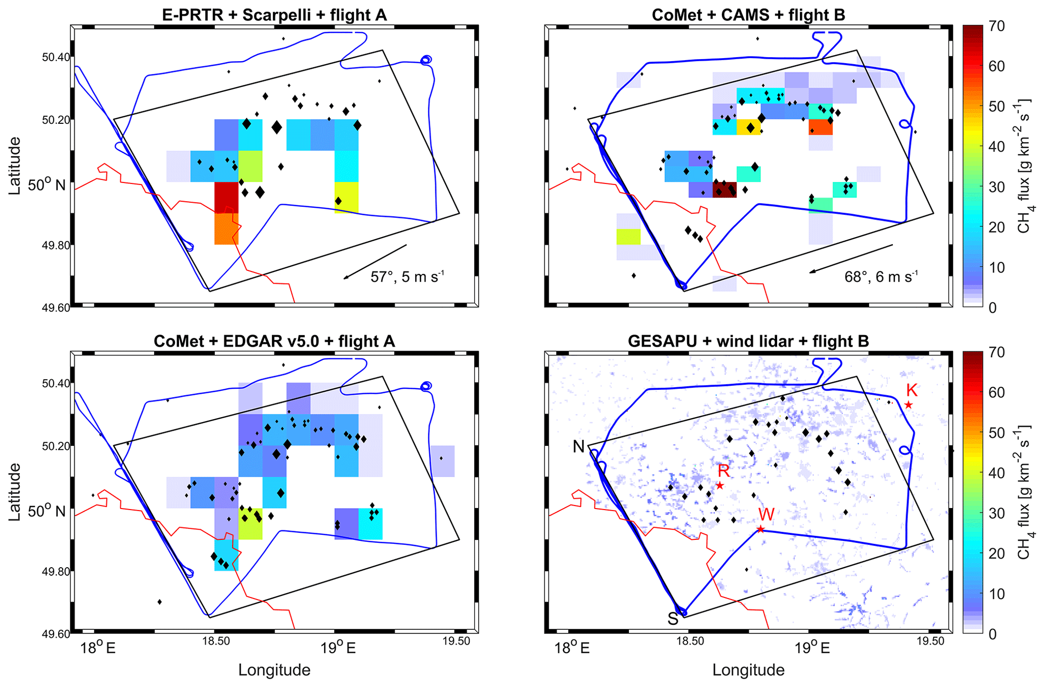
Figure 2CH4 emission distribution of inventories in the USCB. Background colors give emissions from gridded inventories Scarpelli, CAMS, EDGAR and GESAPU, while the markers are sized according to the emissions of the point source inventories E-PRTR and CoMet. Additionally, we added GESAPU sources above 1 kt a−1 CH4 as markers for better visibility. The black boxes denote the emission area for comparison with the mass balance estimate via aircraft. The blue lines show the flight tracks of the flights A and B on 6 June 2018, used in the mass balance, and the arrows in the top two panels show the mean wind direction during the two flights. The red line denotes the Polish–Czech border. Red stars in the bottom right panel show the locations of the wind lidar instruments (R: Rybnik; W: Wiłsa Mala; K: Krzykawka). Also marked in this panel are the southern and northern edges of the downwind wall S and N.
The concentration enhancements Δc are calculated from observed, interpolated mole fractions m and the background mole fraction m0 of the trace gases using linear temperature and pressure profiles deduced from the airborne measurements:
Here, M is the gas molecular weight, p the pressure, R the universal gas constant, and T the temperature in kelvin.
To retrieve trace gas mole fractions m and wind speed v on the wall between the actual flight tracks, we use the kriging interpolation method with a stochastic Gaussian model. Kriging creates a grid of estimated values from data points with sparse spatial coverage and also gives standard errors for these values. We use a modified version of the EasyKrig software (© Dezhang Chu and Woods Hole Ocean Institution). For more details see Mays et al. (2009) and Pitt et al. (2019), who previously used this software in an aircraft mass balance study.
For CH4, not only the mole fraction measured along the flight transects but also the data of the ground-based measurements are included in the kriging. Although CO2 was also measured on the ground by the same instruments, the data cannot be used because they are heavily influenced by the surrounding car traffic. For ground-based CO2, neither large-scale enhancements nor background concentrations could be discerned. We chose the CH4 observations along the ground track closest in time to the airborne measurements. The data are projected onto the downwind wall, averaged over 20 s and then interpolated horizontally to regular distances before kriging. Airborne data are averaged over 10 s intervals in order to reach similar spatial resolution to the ground-based data. Only data below the PBLH are included in the kriging process. We then closely followed the approach described in Pitt et al. (2019). The kriging output fields of CH4, CO2, CO mole fractions and perpendicular wind speed are given at a grid resolution of 0.1∘ in latitudinal direction and 20 m in the vertical.
2.2.1 Downwind and upwind background determination methods
For the mass balance approach, the background mole fraction m0 of the trace gases needs to be determined. Here we compare two methods: (i) background estimated from the downwind wall's edges and (ii) background estimated from the upwind leg. The downwind background method assumes that the boundary layer height remains constant for the time of sampling within the wall, while the upwind method requires the boundary layer to stay at the same height for the whole flight time and ideally a quasi-Lagrangian sampling of the same air mass in the upwind and downwind transects. Thus, the less strict criteria of the downwind background method are more likely to be met in real conditions, and we will use this method in our best estimate and the upwind background as a sensitivity test. The downwind method also requires that there are no sources upwind of the area of interest which would create a complex concentration pattern flowing into the domain. To show this we used our upwind flight transect similar to previous studies (Karion et al., 2013; Heimburger et al., 2017).
In order to determine the downwind background mole fraction from the wall's edges, we evaluate the variability of the CH4 observations within the PBL. The background is separated from the plume using the standard deviation within a 2 min interval for airborne and 10 min interval for ground-based data. Starting at the edges of the wall, the interval is moved towards the center. We define the boundary between CH4 atmospheric background and plume where the standard deviation surpasses 3.4 ppb CH4. The average CH4 background standard deviation is 2.9 ppb. The CO2 background section is adopted from the CH4 background, because the variability in the background is too high for this approach to be applicable. The CO background threshold for the 2 min interval is 4.5 ppb with an average background standard deviation of 3.5 ppb. We average all background mole fraction observations within the PBL to the south and north of the plume separately. The mean of these two values is considered to be the average background for the downwind method. Thus, we assume a linear spatial gradient in the trace gas background.
The second way of determining the atmospheric background mole fraction uses the observations within the boundary layer from the upwind flight transect, which was flown about 15 min before the downwind wall and is here used in a sensitivity study. Methodologically, we define a perpendicular inflow transect according to the prevalent wind direction and project the upwind measurements onto this line (Supplement Fig. S1). After interpolation to regular distances, the average inflow mole fraction represents the upwind trace gas background. This approach has the advantage that sources upwind of the area of interest can be identified through potential enhancements in the upwind transect and are excluded from the emission estimate. On the other hand, the upwind background assumes that the same air masses are sampled in the up- and downwind, which is not true for our two flights, since the air masses needed approximately 3–4 h to travel from the upwind to the downwind measurement location, while the aircraft only needed 15 min. The maximum time separation between up- and downwind sampling is 1.5 h. Thus, our sampling is not strictly Lagrangian (i.e. air mass following), and changes in boundary layer background concentrations over time may affect the emission estimates using the upwind background method. Another disadvantage of using upwind background concentrations with respect to CO2 is the necessity to account for large-scale ground fluxes like the biogenic uptake of CO2, which is discussed in the next section.
2.2.2 Simulation of biogenic uptake of CO2
We derive the influence of biogenic uptake of CO2 from a combination of backward trajectories, calculated using the Stochastic Time-Inverted Lagrangian Transport (STILT; Lin et al., 2003) model and biospheric fluxes from the Vegetation Photosynthesis and Respiration Model (VPRM; Mahadevan et al., 2008). STILT was set up with receptors distributed along the flight track of the downwind wall and from each receptor, we then release 100 particles in the model. To drive the trajectory simulations, we used output of the ECMWF HRES short-term forecasting system (approx. 9 km ×9 km spatial resolution, 137 vertical levels), preprocessed to assure mass conservation of the wind fields. The median locations of the particle ensemble then constitute the median trajectories (Fig. S2). The optimal use of the model in the method described would require the upwind track to be flown in exactly a Lagrangian manner, sampling the same air mass upwind and downwind of the sources. In our case, we have a single hour of temporal difference in the observations and a 4 h difference in the air-mass flow between measurement locations, during which the biosphere was able to uptake CO2. For the difference in background mole fractions, the hour of biogenic uptake between upwind and downwind observations is relevant. The biospheric VPRM contribution to the downwind measurements is calculated using the footprint derived from the last hour of each trajectory, multiplied with the VPRM fluxes corresponding in time and location. We decided on this hybrid approach, in which we assume that we can still link the measurements to our model quasi-directly, despite the fact that the model results are simulated for a location several tens of kilometers away from the actual upwind measurement location. It should be noted that it is assumed here that the biospheric fluxes are spatially homogeneous. We add this contribution to the downwind CO2 observation, only when using an upwind background, and then we use these values for the interpolation with kriging.
2.3 Error estimate
For an error estimate of the derived mass flux, we consider the statistical error of the input data and the systematic error of the method.
2.3.1 Statistical error
The statistical error of our approach is determined using error propagation in the flux equation (Eqs. 1–2). The uncertainty calculation of the concentration enhancement uΔc, the flux density uncertainty uFd and the final flux uncertainty uF are described by Eqs. (3)–(5):
The first two uncertainties are calculated for each grid point of the wall surface; the final flux uncertainty uF is the combination of the single uncertainties. The trace gas uncertainty uc and wind speed uncertainty uv are a combination of measurement and kriging uncertainties expressed as kriging standard error (KSE):
The measurement uncertainty umeasurement has been determined to 1.1 nmol mol−1 (hereafter referred to as parts per billion) for CH4, 0.15 µmol mol−1 (hereafter referred to as parts per million) for CO2 (Table S2, Sect. S1) and 7 ppb for CO (Kostinek et al., 2019). The wind speed measurement uncertainty uv has been assessed to be 0.3 m s−1 for each of the horizontal components (Mallaun et al., 2015). The uncertainty of the interpolation and extrapolation kriging method is output by EasyKrig as a gridded field of normalized variance values ukriging. To retrieve the gridded KSE (see Fig. S4), which is equivalent to the standard deviation, we multiply the kriging error output ukriging by the variance of the kriging input dataset Δc and then take the square root (Eq. 6). The background mole fraction uncertainty is here defined as the standard deviation of all data points contributing to the background calculation (see Table 4). The uncertainty of the grid cell area A is assumed to be zero.
2.3.2 Systematic error
We conducted several sensitivity tests in order to test the robustness of our mass balance method and to determine its systematic error. These sensitivity tests are described and discussed in Sect. 3.4. We assume all systematic errors to be independent and calculate the total absolute systematic error as the square root of the sum of squared individual differences from the best estimate, which treats the data as described in Sect. 2.2 with a downwind trace gas background.
2.4 Bottom-up emission inventories
Several inventories of greenhouse gas and air pollutant emissions exist for the USCB. They vary in spatial and temporal resolution, as well as in the time for which they are available. Table 1 gives an overview of the six inventories we use in this study for comparison with top-down-derived CH4, CO2 and CO emissions in the USCB region.
Table 1Overview of emission inventories used in this study. The year states the last year for which data are available.

The first point source inventory listed in Table 1 is the European Emission Release and Transfer Register (E-PRTR). It results from the regulation (EC) no. 166/2006, which implements the United Nations Economic Commission for Europe (UNECE) PRTR Protocol under which industrial facilities have to report their emissions to air if they exceed a threshold of 100 t a−1 for CH4, 100 kt a−1 for CO2 and 500 t a−1 for CO. Annual data can be downloaded from the European Environmental Agency's website (EEA, 2020). More information on the E-PRTR is given via its website: https://prtr.eea.europa.eu/ (last access: 24 February 2020).
The CoMet v2 inventory is a point source inventory based on the E-PRTR 2016 emissions created by the CoMet team especially for this campaign. It comprises anthropogenic sources of CH4 and CO2 in the USCB and its vicinity. The largest difference between the E-PRTR and the CoMet inventory is that E-PRTR considers each coal mine to be one single point source, often located at the mining operator headquarters, whereas in the CoMet inventory individual ventilation shafts were visually geo-localized using Google Earth. Then, the emission value of each mine was evenly distributed between all ventilation shafts belonging to that mine. Active Czech coal mines in the Ostrava region did not report any CH4 emissions to E-PRTR but were assumed to emit the same amount of CH4 per metric ton of extracted coal as Polish mines. We deduced a factor of 11.8±5.2 kg CH4 per metric ton of extracted coal for the USCB mines listed in Table S3 and applied this value to the Czech mines of Karviná, Karkov, CSM and Paskov. The locations of the 14 listed landfills and waste disposal sites were checked against satellite imagery. Their CH4 emission is assumed to be 3.3 kt a−1, which is less than 1 % of the total USCB emissions.
Scarpelli et al. (2020) published the newest gridded emission inventory available for comparison within this study. It only contains CH4 emissions from oil, natural gas and coal exploitation. But since these are the main sources (87 % according to CAMS) of CH4 emissions in the USCB, values are comparable to the total of other inventories. Scarpelli et al. (2020) use the national totals of emissions reported to the UNFCCC and distribute them according to the positions of relevant infrastructure. Uncertainties of the emissions are based on the emission factor uncertainties from the Intergovernmental Panel on Climate Change (IPCC) and are given as gridded information. Averaged over the USCB, the given relative error standard deviation for CH4 emissions is 60.9 %.
The Copernicus Atmospheric Monitoring System (CAMS) regional emission inventory (CAMS-REG-GHG/AP; Granier et al., 2019) is based on the TNO-MACC inventories (Kuenen et al., 2014). This inventory offers a resolution twice as high as the Scarpelli and EDGAR inventories. The inventory was also constructed by using the reported emission national totals by sector and spatially distributing them consistently across all countries by using proxy parameters.
The most widely used gridded emission inventory is probably the Emission Database for Global Atmospheric Research (EDGAR, https://data.europa.eu/doi/10.2904/JRC_DATASET_EDGAR, last access: 22 October 2020) global emission inventory. The most recent version 5.0 (https://edgar.jrc.ec.europa.eu/overview.php?v=50_GHG, last access: 22 October 2020) includes emissions of the three major greenhouse gases CO2, CH4 and N2O. It is based on the previous EDGAR version 4.3.2 (Janssens-Maenhout et al., 2019). We use the CO emissions from the air pollutant inventory (Crippa et al., 2018) from version 4.3.2. The most recent year of emission data is 2015 for CH4, 2018 for CO2 and 2012 for CO. In EDGAR, annual country-specific emissions are derived from international activity data and emission factors, which are then distributed in time and space using monthly shares and spatial proxy datasets. The data include uncertainty factors per species for three types of countries: OECD countries of 1990, countries with economies in transition in 1990 and the remaining countries in development. European emissions from EDGAR in 2012 have standard deviations of 16 % for CH4, 2.5 % for CO2 (Janssens-Maenhout et al., 2019) and 65 % for CO (Crippa et al., 2018).
The GESAPU inventory (Bun et al., 2019) has been created for Ukraine and Poland only for the reference year 2010. Originally, it is a point, line and area source inventory based on shapefiles. The advantage of this type of information is that it has a very high resolution but can also be gridded with any spatial resolution and orientation. The GESAPU inventory comprises all sectors of anthropogenic emissions. Here we use a gridded version of the emissions with a resolution of 15 arcsec (approximately 296 m×463 m for the region).
Figure 2 shows the spatial distribution of CH4 emissions as given by the six inventories. Point sources from E-PRTR and the CoMet inventory are displayed as black markers while the background colors give the gridded inventory values. Although the inventories generally agree on the locations of CH4 emissions, there are several cases where sources seem to be missing. Regarding point sources, E-PRTR (top left) has fewer individual sources than the CoMet inventory (top right) due to the separation in single ventilation shafts. Additional mines in the CoMet inventory include the four Czech mines and the four ventilation shafts of the Brzeszcze mine around 19.15∘ E and 49.95∘ N. The gridded Scarpelli (top left) emission distribution for CH4 does not represent the point sources well. There are no emissions north of 50.2∘ N although several mines are located in this northern area. Generally the CAMS (top right) emission maxima seem to represent the point source locations better than the Scarpelli or EDGAR (bottom left) emission distribution, with the exception of the Czech mines, which are included in Scarpelli and EDGAR, but not in CAMS. In the GESAPU inventory, the high CH4 emissions associated with mining activities were visualized by overlaying a marker for sources above 1 kt a−1 on the gridded emission map. These are fewer high-emitting sources than in the E-PRTR inventory. This could be caused by consolidation and separation of mines between 2010 and 2017, the respective years for the data. Two flights (on 6 June 2018), which are shown as blue tracks in Fig. 2, were designed to capture the emissions of the region during northeasterly wind conditions.
The CO2 and CO emission distribution in the inventories is displayed in Fig. 3. CO2 point sources (from E-PRTR and CoMet) agree well with EDGAR and CAMS, except for the strong CO2 and CO emissions associated with the Łagisza power plant and ArcelorMittal steel factory at 50.34∘ N and 19.28∘ E, which are correctly placed in the northeast corner of the flight track in E-PRTR, CoMet and GESAPU. Instead, EDGAR and CAMS include an emission hot spot to the southeast and east, respectively, of this location that is not associated with a point source. The Rybnik power plant, located in the central western USCB, is the strongest point source emitter of CO2 in all inventories. CO has one emission hot spot in the USCB, namely the ArcelorMittal steel factory next to the Łagisza power plant with 137 kt a−1 in E-PRTR 2017. This source is not represented in EDGAR and shifted to the east in CAMS. GESAPU includes this source, but with much lower emissions of 63 kt a−1.
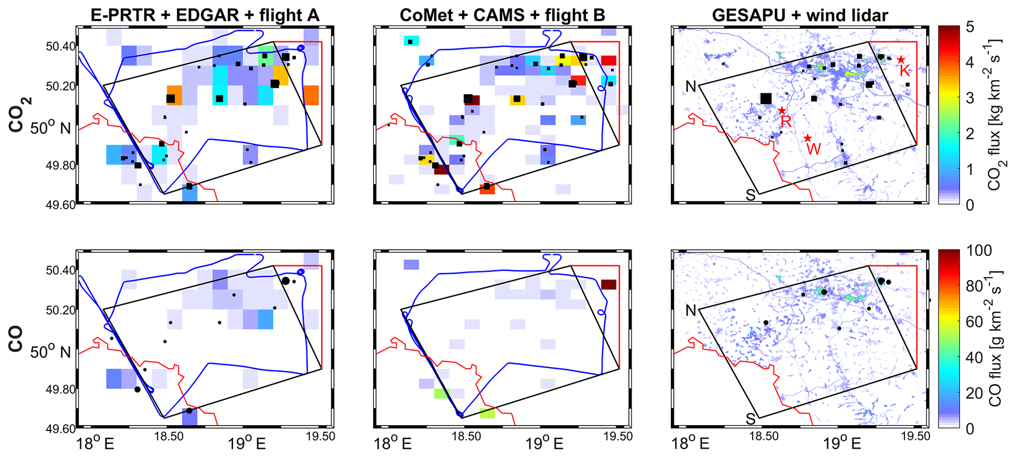
Figure 3Like Fig. 2 but for CO2 and CO. GESAPU sources above 0.1 Mt a−1 and 1 kt a−1 for CO2 and CO, respectively, are added as markers. The straight red lines show the addition to the mass balance area necessary because of misplaced sources.
To compare the emission inventories with our mass balance flights, the emissions of each inventory are summed up within an area representative of the flight track and wind direction (more details see Sect. 3.3), which is marked by the black boxes in Figs. 2 and 3. Since some of the CO2 and CO sources are obviously misplaced in the gridded inventories, but really lie within our mass balance area, we enlarged the mass balance area toward the east in order to include these sources into the USCB sum. These enlargements are marked by red lines in Fig. 3. Although missing sources influence the comparison between inventories and the emission estimate via aircraft, the misplacements might not, since misplaced emissions are now within the enlarged mass balance area.
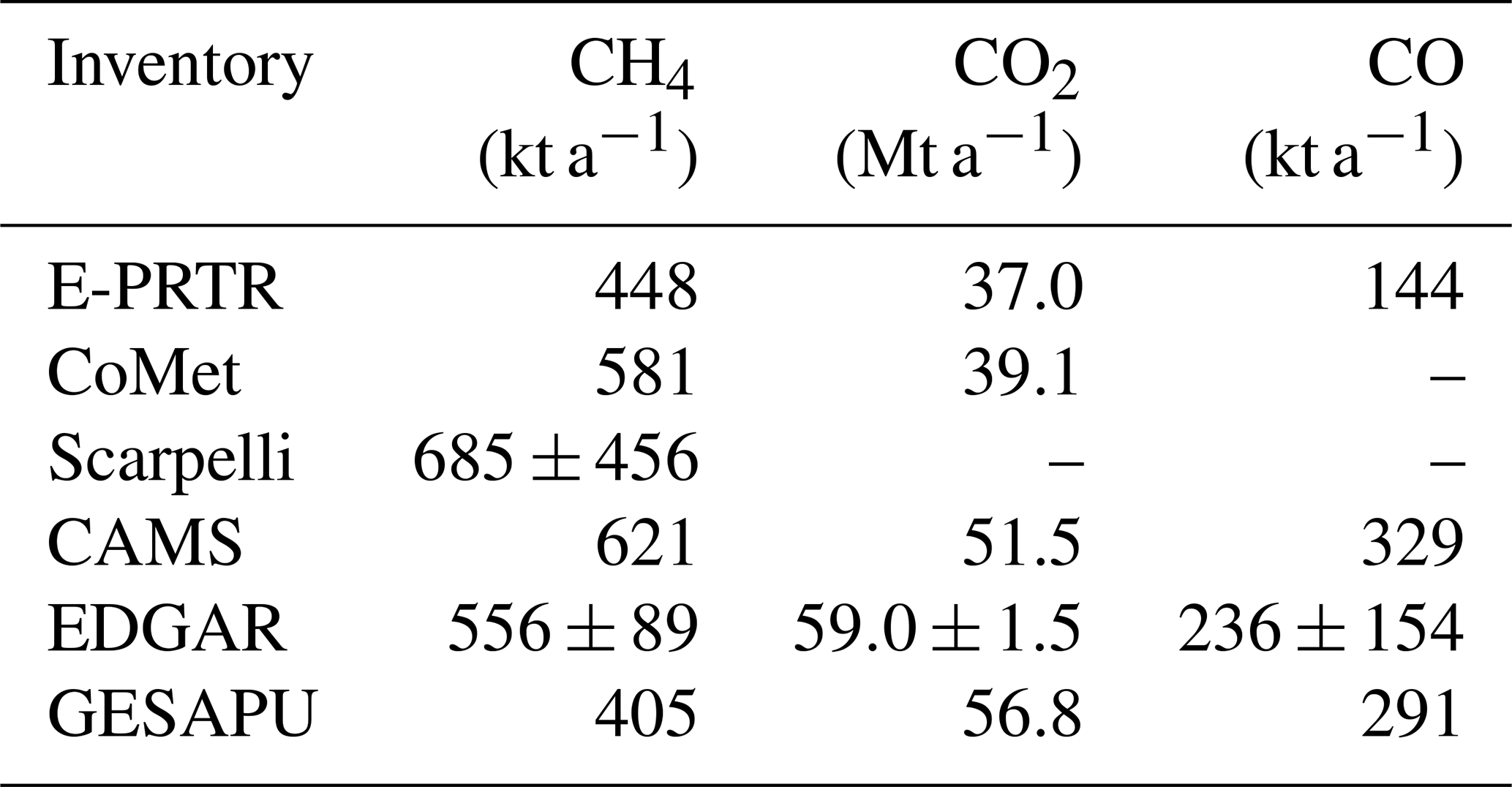
For each inventory, the total annual emission from the enlarged area including the reported uncertainty is given in Table 2. These values include emissions from all sectors available in the inventories (see also discussion in Sect. 4). Scarpelli assumes the highest emissions for CH4, followed by CAMS and CoMet. GESAPU features the lowest CH4 emissions, which might partly arise from the sources in the Czech Republic, which are not covered in the inventory. The highest CO2 emissions are assumed by the EDGAR inventory. CO emissions are highest in CAMS, closely followed by GESAPU.
Table 2Annual emission totals in the USCB area for different emission inventories and trace gases.
3.1 Meteorological situation
The meteorological conditions have to fulfill certain criteria for a feasible mass balance calculation. On 6 June 2018, the weather conditions for an airborne mass balance experiment in the USCB were advantageous due to relatively constant wind speed and wind direction over the sampling time. The PBLH changed considerably during flight A in the morning, but was rather constant during flight B in the afternoon.
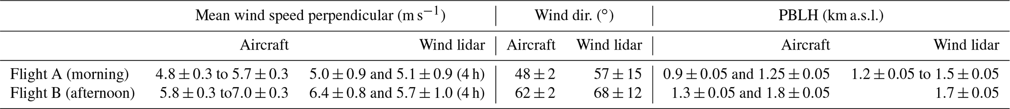
The wind lidar measurements at Rybnik airport were located close to the center of our in situ wall (Fig. 2) and can be used to assess the wind history over the entire measurement day. Vertical profiles of wind speed and wind direction show that during the previous night a low-level jet blew over the area with wind speeds of more than 10 m s−1; in the morning the wind slowed down to around 5 m s−1 and then accelerated to 6–7 m s−1 around 13:00 UTC (Fig. 4, Table 3). The boundary layer wind direction was between 50 and 70∘ over the entire day. The nightly low-level jet prevented accumulation of emissions, and the slowing down around 06:00 UTC provided relatively constant wind speeds for 4 h before we started our downwind sampling at 10:00 UTC. This steady wind history prior to the flight is crucial for the mass balance approach, because of the assumptions stated in Sect. 2.2. During this time emissions from the farthest shafts (75 km from downwind wall) were able to travel from emission to observation location at constant wind speed and direction. A comparison of aircraft observations in the downwind wall and wind lidar averages during the observation times is given in Table 3. Observed wind speeds with the lidar are within the range of aircraft-observed wind speeds. Generally wind speeds in the southern USCB were about 1 m s−1 higher than in the northern part of the USCB.
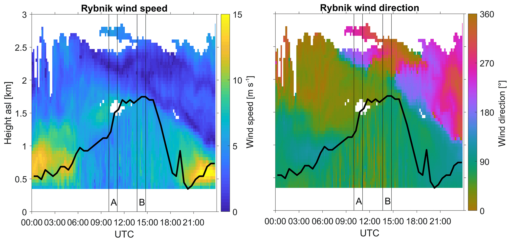
Figure 4Wind speed and direction at Rybnik measured with a Doppler wind lidar on 6 June 2018. The bold line denotes the PBLH determined from the eddy dissipation rate and the thin vertical lines illustrate the downwind wall sampling times of flights A and B.
Table 3Overview of wind data and PBLH from aircraft averaged within the downwind wall and wind lidar observations at Rybnik. Aircraft data give uncertainty ranges due to measurement uncertainty, and wind lidar data state a standard deviation of the measurements within the PBL. The wind speed obtained from the lidar is additionally as an average over the 4 h previous to the downwind sampling.
The diurnal development of the PBLH, with a maximum of 1.7 km above sea level (a.s.l.), is discernible from the wind lidar observations. The PBLH measured by the wind lidar increased from 1.1 to 1.5 km during the sampling of flight A but remained relatively constant at 1.7 km during flight B. We also determined the PBLH from two vertical aircraft profiles of potential temperature, observed before and after the sampling of the downwind wall (Fig. S3). Before flying the wall pattern, we obtained a vertical profile in the southern part of the USCB area (around 49.8∘ N, 18.2∘ E). After finishing the wall pattern a northern profile was sampled on the way back to Katowice airport (50.3∘ N, 18.2∘ E). During both flights, the PBLH was about 400 m lower in the southern part than in the northern part of the USCB. Thus, the PBLH data in Table 3 describe a latitudinal gradient for the aircraft and temporal changes from the wind lidar.
Furthermore, for the mass balance, we assumed no entrainment from the free troposphere during sampling time. This assumption is supported by a strong capping inversion at the PBLH observed in the aircraft profiles (Fig. S3). Still, since the PBLH was increasing during the sampling for flight A, there was considerable entrainment of free-tropospheric air into the mixed layer. The correction we applied for this temporal change of the PBLH is described in the following section. The uncertainty related to this correction is assessed in the sensitivity test (Sect. 3.4) concerning the temporal PBLH variability.
3.2 Kriging results
For our mass balance, we use airborne in situ observations from two flights on 6 June 2018. CH4, CO2 and CO enhancements were clearly observed in the downwind wall. The ground-based teams drove below the upwind and downwind legs using the closest highways and national roads. Halfway through the southern track we ascended and descended to derive the height of the PBL based on meteorological measurements. Above the PBL, observed CH4 and CO concentrations were lower than within the PBL, while CO2 concentrations were higher.
In a first step of emission estimation for the entire USCB (as described in Sect. 2.2) the observed data in the downwind wall are inter- and extrapolated using the kriging algorithm (Fig. 5). Details of the kriging parameters can be found in the Supplement (Sect. S2). Mole fractions in the wall are cut off below the ground, above the PBL, and to the south and north of the flight legs (points S and N).
For the morning flight A, the trace gas plumes reach from the ground to the top of the PBL. The transects on the ground and at 800 m show the highest CH4 maxima (Fig. S4). At 1000 and 1100 m the maximum enhancements are lower. The same is true for the CO2 and CO enhancements. This is probably caused by the growing PBLH during the flight. During the downwind measurement of the morning flight A, the height of the PBL increased from 1.2 k a.s.l. (0.9 km above ground level, a.g.l.) to 1.5 km a.s.l. (1.2 km a.g.l.), which is an increase of 20 %. The lowest transect (800 m) was sampled first in the shallowest PBL. The two upper transects were sampled about half an hour later, when the PBLH had increased by about 20 %. Thus the emissions from the USCB were mixed within a much smaller volume during the lowest transect than during the following two. The ground-based sampling of the morning flight took place between 09:00 and 10:40 UTC. Two cars started in the center of the downward projected flight track and moved away from each other to the south and north. Thus, the central part was sampled first, during low-PBLH conditions. To account for the low PBLH during the first flight transect and the ground-based sampling, we apply a correction factor of −20 % to the ground observations and the lowest flight transect. Figure S4 shows the original, uncorrected observational data, while Fig. 5 shows the corrected values. Corrected enhancements are on the order of 0.16 ppm CH4, 7 ppm CO2 and 130 ppb CO.
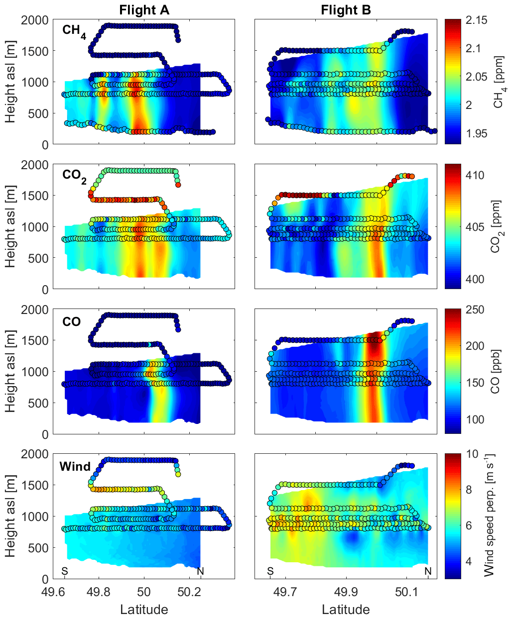
Figure 5Mole fractions and perpendicular wind speed in the downwind in situ wall from observations (circles) and inter- and extrapolation with a kriging algorithm (shading). The CH4 wall incorporates ground-based measurements. For CO2 and CO the ground mole fraction is assumed to be the same as in the lowest flight track. The wind extrapolation does not use any information below the lowest flight track.
During the afternoon flight B, the CH4 plume is evenly distributed between the ground observations and the lowest flight track at 800 m (Fig. 6). Thus, we assume good vertical mixing within the PBL and use the same CO2 and CO mole fractions at the ground as in the lowest flight transect. Trace gas enhancements are on the order of 0.12 ppm CH4, 6 ppm CO2 and 120 ppb CO, thus lower than during the morning flight. The main CH4 plume is located at 50.0∘ N with a secondary plume around 49.8∘ N. There are two CO2 plumes at 50.0 and 50.1∘ N. The CO plume is located at 50.0∘ N.
The horizontal wind speed shows a latitudinal gradient with higher wind speeds in the south than in the north for both flights. This gradient is preserved when using a kriged wind field for flux calculation instead of an average wind speed for the whole downwind wall (as discussed in Sect. 3.4).
Error estimates from the interpolation and extrapolation are retrieved from the kriging software as gridded fields (see Fig. S5). The KSE generally increases with distance to the measurement locations and is highest at the ground for CO2, CO and wind speed because no ground-based measurements were available for these parameters.
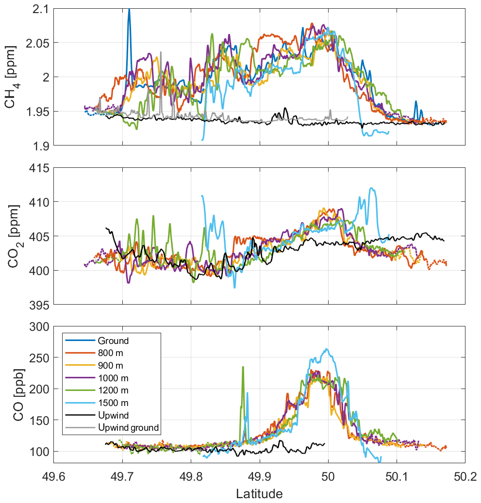
Figure 6Mole fractions of CH4, CO2 and CO at different heights above mean sea level within the PBL downwind of the sources for flight B. Background mole fractions according to the downwind method are displayed as the dashed part of the lines at the edges. Additionally, the background according to the upwind method is shown in black and grey. Upwind data have been shifted to the respective downwind latitude. The CO upwind background stops at 50∘ N due to an instrument startup delay on this part of the track.
3.3 Background mole fractions
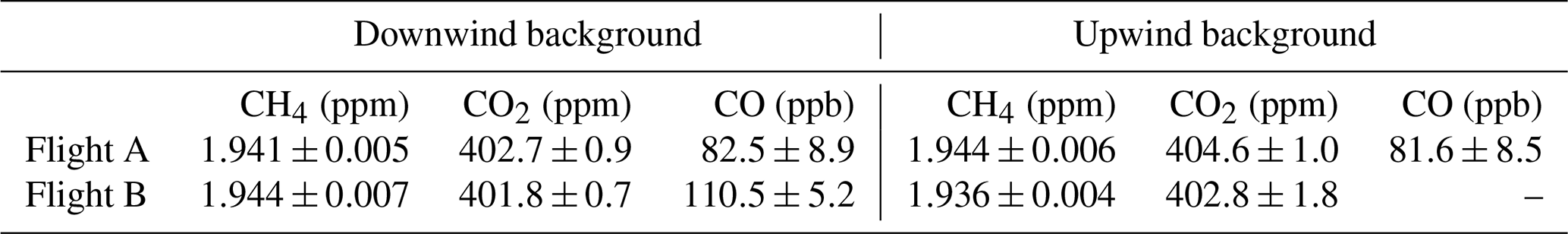
We applied both the downwind and the upwind methods (see Sect. 2.2.1) to determine atmospheric background mole fractions of trace gases. Average background mole fractions and standard deviations for both methods are summarized in Table 4. Figure 6 shows the observed PBL mole fractions of CH4, CO2 and CO at different heights for flight B. The highest transect (light blue), originally planned in the free troposphere above the PBL turned out to partially be within the PBL, but the southern and northern ends were sampled in the free troposphere. The background mole fractions according to the downwind method are displayed as dotted lines. For flight A, the background could not be reached to the south of the downwind wall, and only background values from the north were used for CH4 and CO2 (Fig. S4).
Table 4Average background mole fractions and their standard deviations calculated with the downwind and upwind methods.
The upwind mole fractions (black lines) were shifted to the corresponding latitudes of the downwind wall based on the wind direction. The CH4 upwind mole fractions follow the same north–south gradient as the downwind background (Fig. 6, top). Around 49.94∘ N the CH4 mole fraction is slightly enhanced in the upwind. There is a similar enhancement around 50.13∘ N in flight A (Fig. S4). Due to the projection, these would be between 50.2 and 50.3∘ N on the inflow track. The only source upwind of the inflow track in the inventories is the Trzebinia mine and power plant at 19.44∘ E and 50.16∘ N. We use the ground-based observations below the upwind track (grey line) to confirm our aircraft observations. They show similar absolute values and a similar north–south trend to the airborne track. Additionally, there are three spikes between 49.73 and 49.78∘ N. These locations correspond to an inflow latitude of around 50.0∘ N and probably originate from sources close by, since they do not appear in the airborne observations. The largest peak most likely originates from the coal processing and waste water treatment facilities right upwind of the measurement route at 50.027∘ N and 19.438∘ E.
The CO2 upwind background is higher than downwind mole fractions at both ends of the measurement transects but lower in the center, where the downwind plume was observed. The average upwind background of CO2 is 2 and 1 ppm higher than the downwind background for flights A and B, respectively. This discrepancy is caused by the biogenic uptake of CO2 between the upwind and downwind transects. The impact of the biogenic sink is discussed below.
Upwind CO observations during flight B do not cover the complete transect due to a start delay of the QCLS. Thus, we did not use the CO upwind background for this flight. The CO upwind observations for flight A show small variations resulting in a background standard deviation of about 9 ppb. Here, the upwind CO measurements are smaller than downwind background values.
The upwind background method calls for an estimate of the biogenic uptake of CO2. We estimate this uptake from the STILT trajectories and the VPRM model (see Sect. 2.3.2). Figure S2 exemplary shows the truncated trajectories for the 800 m altitude transect of flight B. Trajectories for other transects and flight A are very similar. The biogenic uptake for each trajectory is determined from the last hour of transport. By subtracting the VPRM uptake from the corresponding downwind measurement (as the uptake is negative), one can obtain a downwind CO2 concentration without biospheric influence. This uptake is on average 1.00 ppm for flight A and 0.95 ppm for flight B.
3.4 USCB emission estimate
From the two mass balance flights on 6 June 2018, we determined the total USCB emissions of CH4, CO2 and CO. Figure 7 summarizes the best-estimate emissions and the sensitivity calculations (see Sect. 2.3). The uncertainty of the best-estimate includes the statistical error, calculated from the uncertainties of the input parameters and the systematic error calculated from the sensitivity tests. The CH4 emission estimates for the entire USCB on 6 June are 13.8±4.3 and 15.1±4.0 kg s−1 for flights A and B, respectively. This is a difference of 9 % between the two flights. The CO2 emission estimates are 1.21±0.75 and 1.12±0.38 t s−1 for the two flights, also with a difference of 9 %, but with the morning flight results being higher. Finally, CO emissions from the USCB were calculated to be 10.1±3.6 and 10.7±4.4 kg s−1 for flights A and B, respectively. The discrepancy between them is 6 %.
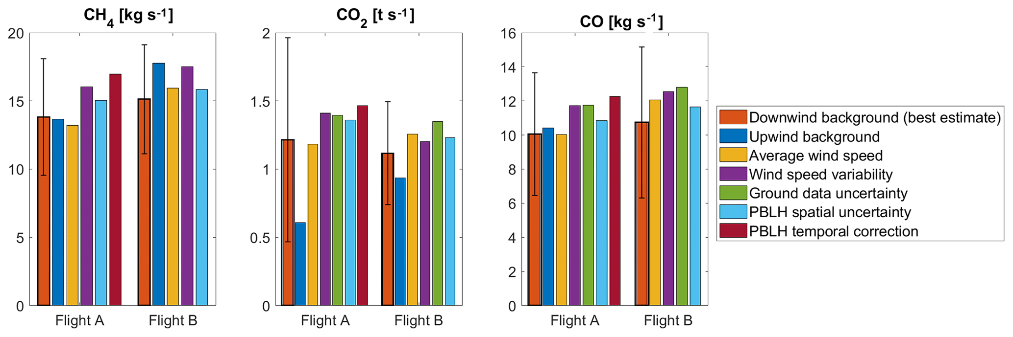
Figure 7USCB emission estimates on 6 June 2018, using an airborne mass balance approach including several sensitivity tests.
We determined the systematic errors with several sensitivity tests applied to the treatment of different variables during the mass balance calculation (Fig. 7). Systematic errors are calculated as the emission difference between the best estimate mass balance using downwind background as described in Sect. 2.3 and the sensitivity studies.
-
Upwind background method
This background method leads to almost the same CH4 emission estimate for flight A. The flight B estimate is 18 % larger than the best estimate, showing that the assumption of a linear background gradient is not true for this case. The CO2 emission estimate using an upwind background is 50 % and 16 % smaller than the best estimate for flights A and B, respectively. Especially for flight A, the upwind CO2 mole fractions in the PBL might be enhanced due to a shallower PBLH. Also, the experiment was not conducted in a Lagrangian way, meaning that the sampling time difference between upwind and downwind does not match the travel time of the air. With potentially inhomogeneous biosphere–atmosphere fluxes, this could cause a problem. For CO the upwind background method yields an emission estimate difference of 3 % for flight A. For flight B we did not calculate a CO emission estimate because of an incomplete upwind measurement (Fig. 6). In general, CO upwind and downwind background data are quite similar.
-
Average wind speed
The impact of wind measurement treatment on the estimated mass fluxes was tested by using the averaged observed wind speed instead of the kriged wind field. This technique could for example be employed if no wind measurements were available and average model winds need to be used. The emission estimates for the morning flight are up to 4 % lower and for the afternoon flight up to 13 % higher than for the best estimate. Here the systematic change in the emission estimates is caused by the location of the plume in the wind field. During flight A, the plumes were located where the wind speed was slightly higher than average (see Fig. 5). Using the average wind speed, thus, results in a reduction of the emission estimates. During flight B, the plume locations were in a slow wind region with higher wind speeds to the south, especially for the CO2 and CO plumes. Using averaged wind speed, thus, enhanced the emission estimate. We highlight the importance of measuring the wind speed simultaneously with the mole fractions and using this spatial knowledge in the flux calculation.
-
Wind speed variability
One assumption for a mass balance calculation is that the wind speed and direction are constant during the time it takes for the gases to be transported from the emission source to the observation location. In reality the wind field can be subject to considerable variability. In our case we were able to assess this temporal variability from the wind lidar observations. To account for wind variability we calculated the standard deviation of wind speed during the 4 h transit time within the boundary layer and added it to the kriged wind field used in the mass balance calculation. This introduced an uncertainty of 17 % and 15 % to the morning and afternoon flight results, respectively.
-
Ground data uncertainty
Since we did not use CO2 and CO from the mobile ground measurements, we calculated the sensitivity of our approach to the precise knowledge of ground-based data for CO2 and CO. Assuming a 10 % uncertainty of the ground value enhancements and increasing the kriging input ground values by this factor result in a systematic error of 15 %–20 %. This shows that a good approximation, or even better a measurement, of mole fractions below the lowest flight track is important for exact emission estimates.
-
PBLH uncertainty
Another sensitivity of our method is related to the knowledge of the PBLH and its variability. Its exact determination in the downwind wall is only possible when we cross its top during ascents or descents. This occurred once during the morning flight and three times in the afternoon. The PBLH is further constrained by vertical profiles before and after sampling the downwind wall and through the wind lidar observations. These data hint at temporal and spatial variations in the PBLH (see Sect. 3.1). Based on these data we assign an uncertainty estimate of 100 m to PBLH. We account for the spatial PBLH uncertainty in the emission estimate by using a boundary layer 100 m higher than our best estimate. This is realized through cutting off the flux density field at this increased boundary. For this sensitivity test, discrepancies are between 5 % and 12 % for all three gases.
-
Temporal PBLH variability
The last sensitivity test accounts for the temporal variation in the PBLH during the morning flight A. The PBLH showed a temporal variability of 300 m, quantifiable from wind lidar measurements. We assess the uncertainty caused by the temporally increasing PBLH for the morning flight by omitting the trace gas enhancement correction described in Sect. 3.2. The systematic error for flight A is between 21 % and 23 %.
On average, the uncertainty of the background mole fraction (up to 50 %), the uncertainty of mole fractions at the ground (15 %–20 %) and the wind variability (15 %–17 %) have the highest impact on the systematic uncertainty. For flight A, the changing PBLH introduces an additional 21 %–23 % uncertainty to the emission estimates. Assuming that the single systematic uncertainties are independent of each other, the total systematic error of the emission estimate is calculated as the square root of the sum of squared individual uncertainties and is added to the statistical uncertainty. The statistical error is 1 % for CH4 and around 3 % for CO2 and CO and, thus, small compared to the systematic errors of this approach. It is added to the systematic error to obtain the total error of the emission estimates. The CH4 emission estimate has a total relative error of 31 % and 26 %, a CO2 estimate of 62 % and 37 %, and a CO estimate of 36 % and 41 % for flights A and B, respectively. The errors are mostly larger for flight A than for flight B, since the afternoon flight is more suitable for a mass balance experiment due to the temporally constant PBLH.
3.5 Single-transect emission estimates
This detailed emission estimate, as described above, can help to understand uncertainties of a mass balance study in cases where less information is available. We ensured the validity of the mass balance technique by performing multiple vertical transects and even driving underneath the flight path to capture the signal at the surface layer. Many mass balance studies do not put in this level of effort, hence we can estimate how necessary these extra precautions are with regard to calculating the true emissions. Furthermore, when using mass balance techniques at any point to verify emissions from a policy enactment standpoint, resources should be used as efficiently as possible. By using the information from single transects within the boundary layer of each flight, we calculated the emissions under the simple assumption of a perfectly mixed boundary layer. The PBLH was kept constant for all transects. Figure 8 shows the results of the single-transect mass balance calculations for the two flights on 6 June 2018. The average of the single transects (blue) is always well within the uncertainty range of the kriging mass balance results (red). Nevertheless, by assuming that one individual transect is representative for the entire PBL, transect emission estimates deviate up to 40 % in both directions from the kriging estimate for CH4. This deviation is much larger than the kriging estimate uncertainty. Deviations are largest for transects close to the PBLH when the concentration gradient between the boundary layer and free troposphere is also large, e.g. the highest CH4 transects. Thus, when calculating emissions from single transects the flight altitude should be well below the PBLH to avoid sampling free-tropospheric air masses. On the other hand, these results discourage using single-transect mass balance estimates anyway.
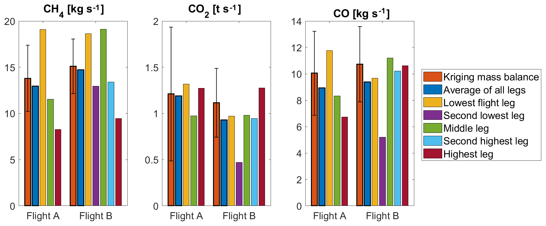
Figure 8Mass balance results for single transects through the plumes compared to the average of all single transects and the kriging mass balance result from Sect. 3.4.
Hereafter we compare our airborne top-down emission estimate for the USCB with the bottom-up emission inventories described in Sect. 2.1. Both emission values, the bottom-up inventory and the top-down mass balance estimate, are based on different methods and assumptions which hamper a one-by-one comparison. In particular differences in the temporal resolution of the two methods create a problem in case emissions are subject to strong temporal fluctuations such as a seasonal or diurnal cycle. Aircraft-borne top-down methods can only provide snapshot emission estimates, which for a comparison need to be scaled to the temporal resolution of the emission inventories. At the same time, bottom-up inventories also include uncertainties, for example in the emission factors, which are often derived from process studies and are then used to derive annual sums. For this comparison, we scale our mass balance emission estimate, based on a snapshot of 1 d in the early summer, to an annual emission estimate. We assume this scaling to be representative, because of the nature of the USCB emissions. In general, coal mining activities continue all year round and the power plants using the excavated coal are continually operated base load facilities. Still, it is known that CH4 emissions from individual ventilation shafts vary on weekly to monthly scales, when mines open new longwall excavation areas and ventilation increases. However, since we study emissions on a regional scale (including ∼35 mines), we argue that emissions from individual shafts vary independently and therefore variations cancel out to a large extent. According to the CAMS inventory (Fig. S6), industrial emissions, including coal mine exhaust, make up 87 % of USCB CH4 emissions, with the waste sector (11 %) and fugitives (2 %) being the other contributors. Thus, we assume our CH4 emission estimate to be largely representative for the entire year. CO2 emissions attributed to public power generation (65 %) and residential heating (6 %) do have an annual cycle. The other contributions include industry (21 %) and transportation (7 %). The CO emissions result in 30 % from residential combustion with an annual cycle with the remainder from public power (3 %), industry (54 %) and road transport (13 %) without an annual cycle. Thus, there is an annual cycle for CO2 and CO and our summer measurements likely underestimate the annual value. Additionally, gridded inventories need to be treated with caution when used in region-specific studies (Janssens-Maenhout et al., 2019). These inventories distribute national emission totals onto a grid using proxy data. Most of the uncertainty of the grid cell level data originates from the uncertainty in the proxy data (Hogue et al., 2016). Furthermore, the comparison of inventories from 2010 with observational estimates from 2018 is not consistent, and we treat comparisons to the GESAPU inventory with caution.

Figure 9Comparison of USCB emission estimates of the CoMet mass balance flights A and B with bottom-up emission inventories. Error bars show 1 standard deviation of the estimates, where available.
Our airborne mass balance CH4 emission estimate on 6 June 2018, of 436±135 and 477±126 kt a−1 for flights A and B, respectively, is in the lower range of inventory emissions (Fig. 9). E-PRTR emission estimates are similar to our estimate, despite the omitted sources with emissions lower than the threshold of 0.1 kt a−1. The CoMet emission inventory is higher than both mass balance estimates, but within the error range of flight B. Compared to E-PRTR from 2017, the CoMet inventory includes several mines in Poland that reported higher CH4 emissions in 2016 than in 2017, three additional Czech mines and four landfills within the mass balance area. Scarpelli, CAMS and EDGAR CH4 estimates are also higher than our mass balance results. The GESAPU inventory states the lowest emissions, which may result from the missing emissions from Czech mines (estimated to be around 70 kt a−1).
Our CO2 aircraft mass balance emission estimates of 38.3±23.6 and 35.2±11.9 Mt a−1 agree with all inventories within the reported errors of the measurements. These errors are large, especially for the morning flight. Under very good conditions it is possible to report results that can inform about the quality of emission inventories, but issues like the biospheric fluxes of CO2 and annual cycles of emissions impede comparisons to annual emission inventory values.
The CO emission estimates of 317±114 and 339±139 kt a−1 from the aircraft mass balance on 6 June 2018 are at the upper end of the emission inventories. Especially the E-PRTR emission estimate for 2017 is much lower than the mass balance result. This point source inventory does not include emissions from the transport and residential sector, which together comprise 42 % of USCB CO emissions according to CAMS (Fig. S6), which explains the discrepancy. CAMS, EDGAR and GESAPU inventories are in the range of the emission estimates, but due to the annual cycle in residential combustion we suspect that these inventories underestimate CO emissions from the USCB.
In times of rising atmospheric concentrations of greenhouse gases and countries trying to reduce their associated emissions, it is important to develop an independent and objective emission monitoring system. During the CoMet campaign the European CH4 emission hot spot of the Upper Silesian Coal Basin (USCB) was sampled by in situ techniques as well as passive and active remote sensing on ground and from aircraft. From two flights A and B around the USCB, conducted on 6 June 2018, combined with vehicle-based ground measurements, we determined a regional emission estimate of CH4, CO2 and CO for the entire USCB using in situ data and a mass balance approach. The plumes of all three trace gases could be observed and separated from the atmospheric background in all downwind transects. For the morning flight A, a trace gas enhancement correction was employed to account for the temporal change of PBLH during the sampling. We employed a kriging algorithm for the interpolation of observed CH4, CO2, CO and wind speed between the flight transects and towards the ground. CH4 ground-based observations confirmed the existence of a well-mixed PBL with similar trace gas enhancements at the ground and in the aircraft transects. From the kriged fields we calculated the USCB emission estimate as the mass flux through the downwind wall for each flight. Using error propagation and several sensitivity tests, we carefully determined the total error of our mass balance approach. The CH4 emission estimate has a total relative error of 26 %–31 %, the CO2 estimate of 37 %–62 % and the CO estimate of 36 %–41 %. These uncertainties are mainly caused by the background determination, wind speed variability and missing knowledge of mole fractions below the lowest flight track for CO2 and CO. The higher uncertainty values apply to the morning flight estimate, because the temporal variation in the PBLH introduced a large error. Thus, we highlight the importance of a constant PBLH over time, knowledge of trace gas mole fractions at the ground and the exact knowledge of background mole fractions. The large uncertainties in the CO2 estimate are dominated by the uncertainties in biospheric CO2 fluxes. These estimates could be improved by performing flights in wintertime, when the biospheric fluxes are negligible. Flights during different seasons would also better constrain the annual cycle in CO2 emissions from the residential sector. The calculation of emission estimates from single flight transects is not advisable, because the single-transect estimates showed deviations from their mean and the kriging method of more than 40 % in both directions.
The CoMet in situ CH4 emissions estimates from 6 June 2018, of 13.8±4.3 and 15.1±4.0 kg s−1 for flights A and B, respectively, are in the lower range of the six presented emission inventories. This agreement of our independent USCB emission estimate with the bottom-up coal mining emission reports indicates that this sector of emissions is well understood and monitored on regional scales. The emissions of CO2 were determined to be 1.21±0.75 and 1.12±0.38 t s−1. The estimate from the second flight constrains the emissions to the lower end of inventory values. The gridded inventories, which report higher emissions than our estimate, do not include an annual cycle in the residential combustion emissions of CO2. This might be reflected in our low summer emission estimate. In general, an airborne mass balance estimate for CO2 on these spatial scales is difficult due to inhomogeneous biospheric uptake. CO mass balance emissions of 10.1±3.6 and 10.7±4.4 kg s−1 for the USCB on 6 June 2018 are much higher than the E-PRTR point source inventory, which does not include residential combustion and road transport emissions and are still in the upper range of the gridded emission inventory values. The comparison between the snapshot top-down emission estimate and annual bottom-up inventories is influenced by the temporal variability of emissions in the USCB. Therefore, additional measurements during different seasons are needed to finally confirm bottom-up emission inventories.
Our airborne in situ mass balance method describes a measurement and evaluation strategy, which can be applied for various emission sources on a local to regional scale. In this case, we provide an independent bottom-up emission assessment for the USCB, which also serves as a point of reference for other state-of-the-art techniques, like airborne lidar and passive spectroscopy. A comparison of in situ and remote sensing emission estimation techniques will follow in future studies.
Independent top-down validation of emissions in industrialized countries can confirm the statistical approaches used in bottom-up inventories. Once facility locations and activity, technology, and abatement information becomes available for other countries or regions, the confirmed emissions from industrialized areas will help to improve global emission inventories used in climate projections. These will in turn help policy makers to develop efficient climate mitigation strategies. Consistent, reliable and timely information on greenhouse gas emissions will allow the implementation, evaluation and management of long-term policies that might allow keeping the global temperature rise below 2 ∘C above preindustrial levels.
The data are accessible on the ICOS ERIC – Carbon Portal under https://doi.org/10.18160/0SFH-JJ93 (Fiehn et al., 2020).
The supplement related to this article is available online at: https://doi.org/10.5194/acp-20-12675-2020-supplement.
AF, JK and ME performed the trace gas measurements, calibrations and data preparation. AF analyzed the data and drafted the manuscript. TK provided shaft-wise E-PRTR geolocation and emission data retrieved from the E-PRTR dataset and the Polish State Mining Authority for 2014. This dataset was updated and expanded by MG to the used version 2. MG, JC and CG provided STILT and VPRM simulations and helpful discussions on biogenic uptake of CO2. TR coordinated the deployment of ground-based measurements and helped with data evaluation and interpretation. HM, MS, PK and JN conducted ground-based in situ measurements in the field during the campaign and collected and shared the data. PJ conducted ground-based observations and supported the aircraft observations through coordinating the airport communications at Rybnik airport. NW took an active part during the campaign deploying the wind lidar and retrieving and providing wind lidar data. CM supervised the wind measurements on board the Cessna Caravan and prepared the data. RB provided a gridded version of the GESAPU emission inventory for the USCB. ALN and PJ devised, set up and supervised the forecasting system that allowed flight planning for the CoMet campaign in the USCB. AF coordinated all CoMet campaign contributions. AR developed the research idea and coordinated the CoMet Cessna campaign operations.
All authors contributed to the interpretation of the results and the improvement of the manuscript.
The authors declare that they have no conflict of interest.
This article is part of the special issue “CoMet: a mission to improve our understanding and to better quantify the carbon dioxide and methane cycles”. It is not associated with a conference.
The authors especially thank DLR-FX for the campaign cooperation, especially the pilots Thomas van Marwick and Philipp Weber and the group of Ralph Helmes, Andreas Giez, Martin Zöger and Martin Sedlmeir. We would like to thank Joseph Pitt for providing an updated version of the kriging package and giving advice on its usage. We acknowledge funding for the CoMet campaign by BMBF (German Federal Ministry of Education and Research) through AIRSPACE. We thank DLR VO-R for funding the young investigator research group “Greenhouse Gases”. The ground-based measurements on vehicles were funded by the European Union's Horizon 2020 Research and Innovation program under the Marie Skłodowska-Curie ITN project Methane goes Mobile – Measurements and Modelling (MEMO2; https://h2020-memo2.eu/, last access: 22 October 2020). The authors acknowledge ECCAD for archiving and distributing the CAMS emission inventories.
This research has been supported by the BMBF (grant nos. FKZ 01LK1701A and FKZ 01LK1701C), the EU Horizon 2020 MEMO2 (grant no. 722479), and the Deutsche Forschungsgemeinschaft (DFG) Priority Program SPP 1294.
The article processing charges for this open-access publication were covered by a Research Centre of the Helmholtz Association.
This paper was edited by Anita Ganesan and reviewed by Anna Karion and Zachary Barkley.
Alvarez, R. A., Zavala-Araiza, D., Lyon, D. R., Allen, D. T., Barkley, Z. R., Brandt, A. R., Davis, K. J., Herndon, S. C., Jacob, D. J., Karion, A., Kort, E. A., Lamb, B. K., Lauvaux, T., Maasakkers, J. D., Marchese, A. J., Omara, M., Pacala, S. W., Peischl, J., Robinson, A. L., Shepson, P. B., Sweeney, C., Townsend-Small, A., Wofsy, S. C., and Hamburg, S. P.: Assessment of methane emissions from the U.S. oil and gas supply chain, Science, 361, 186–188, https://doi.org/10.1126/science.aar7204, 2018.
Amediek, A., Ehret, G., Fix, A., Wirth, M., Büdenbender, C., Quatrevalet, M., Kiemle, C., and Gerbig, C.: CHARM-F – a new airborne integrated-path differential-absorption lidar for carbon dioxide and methane observations: measurement performance and quantification of strong point source emissions, Appl. Opt., 56, 5182–5197, https://doi.org/10.1364/AO.56.005182, 2017.
Barkley, Z. R., Lauvaux, T., Davis, K. J., Deng, A., Fried, A., Weibring, P., Richter, D., Walega, J. G., DiGangi, J., Ehrman, S. H., Ren, X., and Dickerson, R. R.: Estimating Methane Emissions From Underground Coal and Natural Gas Production in Southwestern Pennsylvania, Geophys. Res. Lett., 46, 4531–4540, https://doi.org/10.1029/2019gl082131, 2019.
Bergamaschi, P., Karstens, U., Manning, A. J., Saunois, M., Tsuruta, A., Berchet, A., Vermeulen, A. T., Arnold, T., Janssens-Maenhout, G., Hammer, S., Levin, I., Schmidt, M., Ramonet, M., Lopez, M., Lavric, J., Aalto, T., Chen, H., Feist, D. G., Gerbig, C., Haszpra, L., Hermansen, O., Manca, G., Moncrieff, J., Meinhardt, F., Necki, J., Galkowski, M., O'Doherty, S., Paramonova, N., Scheeren, H. A., Steinbacher, M., and Dlugokencky, E.: Inverse modelling of European CH4 emissions during 2006–2012 using different inverse models and reassessed atmospheric observations, Atmos. Chem. Phys., 18, 901–920, https://doi.org/10.5194/acp-18-901-2018, 2018.
Brioude, J., Angevine, W. M., Ahmadov, R., Kim, S.-W., Evan, S., McKeen, S. A., Hsie, E.-Y., Frost, G. J., Neuman, J. A., Pollack, I. B., Peischl, J., Ryerson, T. B., Holloway, J., Brown, S. S., Nowak, J. B., Roberts, J. M., Wofsy, S. C., Santoni, G. W., Oda, T., and Trainer, M.: Top-down estimate of surface flux in the Los Angeles Basin using a mesoscale inverse modeling technique: assessing anthropogenic emissions of CO, NOx and CO2 and their impacts, Atmos. Chem. Phys., 13, 3661–3677, https://doi.org/10.5194/acp-13-3661-2013, 2013.
Bun, R., Nahorski, Z., Horabik-Pyzel, J., Danylo, O., See, L., Charkovska, N., Topylko, P., Halushchak, M., Lesiv, M., Valakh, M., and Kinakh, V.: Development of a high-resolution spatial inventory of greenhouse gas emissions for Poland from stationary and mobile sources, Mitig. Adapt. Strat. Gl., 24, 853–880, https://doi.org/10.1007/s11027-018-9791-2, 2019.
Cambaliza, M. O. L., Shepson, P. B., Bogner, J., Caulton, D.R., Stirm, B., Sweeney, C., Montzka, S.A., Gurney, K.R., Spokas, K., Salmon, O.E., Lavoie, T.N., Hendricks, A., Mays, K., Turnbull, J., Miller, B.R., Lauvaux, T., Davis, K., Karion, A., Moser, B., Miller, C., Obermeyer, C., Whetstone, J., Prasad, K., Miles, N., and Richardson, S.: Quantification and source apportionment of the methane emission flux from the city of Indianapolis, Elem. Sci. Anth., 3, 000037, https://doi.org/10.12952/journal.elementa.000037, 2015.
Conley, S., Faloona, I., Mehrotra, S., Suard, M., Lenschow, D. H., Sweeney, C., Herndon, S., Schwietzke, S., Pétron, G., Pifer, J., Kort, E. A., and Schnell, R.: Application of Gauss's theorem to quantify localized surface emissions from airborne measurements of wind and trace gases, Atmos. Meas. Tech., 10, 3345–3358, https://doi.org/10.5194/amt-10-3345-2017, 2017.
Crippa, M., Guizzardi, D., Muntean, M., Schaaf, E., Dentener, F., van Aardenne, J. A., Monni, S., Doering, U., Olivier, J. G. J., Pagliari, V., and Janssens-Maenhout, G.: Gridded emissions of air pollutants for the period 1970–2012 within EDGAR v4.3.2, Earth Syst. Sci. Data, 10, 1987–2013, https://doi.org/10.5194/essd-10-1987-2018, 2018.
Cui, Y. Y., Brioude, J., McKeen, S. A., Angevine, W. M., Kim, S.-W., Frost, G. J., Ahmadov, R., Peischl, J., Bousserez, N., Liu, Z., Ryerson, T. B., Wofsy, S. C., Santoni, G. W., Kort, E. A., Fischer, M. L., and Trainer, M.: Top-down estimate of methane emissions in California using a mesoscale inverse modeling technique: The South Coast Air Basin, J. Geophys. Res.-Atmos., 120, 6698–6711, https://doi.org/10.1002/2014JD023002, 2015.
EEA: The European Pollutant Release and Transfer Register (E-PRTR), Member States reporting under Article 7 of Regulation (EC) No. 166/2006, https://www.eea.europa.eu/data-and-maps/data/member-states-reporting-art-7-under-the-european-pollutant-release-and-transfer-register-e-prtr-regulation-18, last access: 22 October 2020.
Fiehn, A., Kostinek, J., Ecki, M., Klausner, T., Gałkowski, M., Chen, J., Gerbig, C., Röckmann, T., Maazallahi, H., Schmidt, M., Korbeń, P., Nȩcki Jarosław, Jagoda, P., Wildmann, N., Mallaun, C., Bun, R., Nicki, A.-L., Jöckel, P., Fix, A., and Roiger, A.: Data supplement to: Fiehn et al. (2020): Estimating CH4, CO2, and CO emissions from coal mining and industrial activities in the Upper Silesian Coal Basin using an aircraft-based mass balance approach (Version 1.00), ICOS Carbon Portal, https://doi.org/10.18160/0SFH-JJ93, 2020.
Granier, C., Darras, S., Denier van der Gon, H., Doubalova, J., Elguindi, N., Galle, B., Gauss, M., Guevara, M., Jalkanen, J.-P., Kuenen, J., Liousse, C., Quack, B., Simpson, D., and Sindelarova, K.: The Copernicus Atmosphere Monitoring Service global and regional emissions (April 2019 version), Copernicus Atmosphere Monitoring Service (CAMS), Research Report HAL-database, hal-02322431, available at: https://hal.archives-ouvertes.fr/hal-02322431 (last access: 27 October 2020), 2019.
Gurney, K. R., Law, R. M., Denning, A. S., Rayner, P. J., Baker, D., Bousquet, P., Bruhwiler, L., Chen, Y.-H., Ciais, P., Fan, S., Fung, I. Y., Gloor, M., Heimann, M., Higuchi, K., John, J., Maki, T., Maksyutov, S., Masarie, K., Peylin, P., Prather, M., Pak, B. C., Randerson, J., Sarmiento, J., Taguchi, S., Takahashi, T., and Yuen, C.-W.: Towards robust regional estimates of CO2 sources and sinks using atmospheric transport models, Nature, 415, 626–630, https://doi.org/10.1038/415626a, 2002.
Hausmann, P., Sussmann, R., and Smale, D.: Contribution of oil and natural gas production to renewed increase in atmospheric methane (2007–2014): top–down estimate from ethane and methane column observations, Atmos. Chem. Phys., 16, 3227–3244, https://doi.org/10.5194/acp-16-3227-2016, 2016.
Heimburger, A., Harvey, R. M., Shepson, P. B., Stirm, B. H., Gore, C., Turnbull, J., Cambaliza, M. O. L., Salmon, O. E., Kerlo, A.-E. M., Lavoie, T. N., Davis, K. J., Lauvaux, T., Karion, A., Sweeney, C., Brewer, W. A., Hardesty, R. M., and Gurney, K. R.: Assessing the optimized precision of the aircraft mass balance method for measurement of urban greenhouse gas emission rates through averaging, Elem. Sci. Anth., 5, p. 26, https://doi.org/10.1525/elementa.134, 2017.
Hiller, R. V., Neininger, B., Brunner, D., Gerbig, C., Bretscher, D., Künzle, T., Buchmann, N., and Eugster, W.: Aircraft-based CH4 flux estimates for validation of emissions from an agriculturally dominated area in Switzerland, J. Geophys. Res.-Atmos., 119, 4874–4887, https://doi.org/10.1002/2013jd020918, 2014.
Hogue, S., Marland, E., Andres, R. J., Marland, G., and Woodard, D.: Uncertainty in gridded CO2 emissions estimates, Earth's Future, 4, 225–239, https://doi.org/10.1002/2015ef000343, 2016.
Janssens-Maenhout, G., Crippa, M., Guizzardi, D., Muntean, M., Schaaf, E., Dentener, F., Bergamaschi, P., Pagliari, V., Olivier, J. G. J., Peters, J. A. H. W., van Aardenne, J. A., Monni, S., Doering, U., Petrescu, A. M. R., Solazzo, E., and Oreggioni, G. D.: EDGAR v4.3.2 Global Atlas of the three major greenhouse gas emissions for the period 1970–2012, Earth Syst. Sci. Data, 11, 959–1002, https://doi.org/10.5194/essd-11-959-2019, 2019.
Karion, A., Sweeney, C., Pétron, G., Frost, G., Michael Hardesty, R., Kofler, J., Miller, B. R., Newberger, T., Wolter, S., Banta, R., Brewer, A., Dlugokencky, E., Lang, P., Montzka, S. A., Schnell, R., Tans, P., Trainer, M., Zamora, R., and Conley, S.: Methane emissions estimate from airborne measurements over a western United States natural gas field, Geophys. Res. Lett., 40, 4393–4397, https://doi.org/10.1002/grl.50811, 2013.
Karion, A., Sweeney, C., Kort, E. A., Shepson, P. B., Brewer, A., Cambaliza, M., Conley, S. A., Davis, K., Deng, A., Hardesty, M., Herndon, S. C., Lauvaux, T., Lavoie, T., Lyon, D., Newberger, T., Pétron, G., Rella, C., Smith, M., Wolter, S., Yacovitch, T. I., and Tans, P.: Aircraft-Based Estimate of Total Methane Emissions from the Barnett Shale Region, Environ. Sci. Technol., 49, 8124–8131, https://doi.org/10.1021/acs.est.5b00217, 2015.
Klausner, T., Mertens, M., Huntrieser, H., Baumann, R., Galkowski, M., Kuhlmann, G., Fiehn, A., Jöckel, P., Pühl, M., and Roiger, A.: Urban greenhouse gas emissions from the Berlin area: A case study on aircraft-based CO2 and CH4 in situ observations in summer 2018, Elem. Sci. Anth., 8, p. 15, https://doi.org/10.1525/elementa.411, 2020.
Kort, E. A., Eluszkiewicz, J., Stephens, B. B., Miller, J. B., Gerbig, C., Nehrkorn, T., Daube, B. C., Kaplan, J. O., Houweling, S., and Wofsy, S. C.: Emissions of CH4 and N2O over the United States and Canada based on a receptor-oriented modeling framework and COBRA-NA atmospheric observations, Geophys. Res. Lett., 35, L18808, https://doi.org/10.1029/2008gl034031, 2008.
Kostinek, J., Roiger, A., Davis, K. J., Sweeney, C., DiGangi, J. P., Choi, Y., Baier, B., Hase, F., Groß, J., Eckl, M., Klausner, T., and Butz, A.: Adaptation and performance assessment of a quantum and interband cascade laser spectrometer for simultaneous airborne in situ observation of CH4, C2H6, CO2, CO and N2O, Atmos. Meas. Tech., 12, 1767–1783, https://doi.org/10.5194/amt-12-1767-2019, 2019.
Krautwurst, S., Gerilowski, K., Jonsson, H. H., Thompson, D. R., Kolyer, R. W., Iraci, L. T., Thorpe, A. K., Horstjann, M., Eastwood, M., Leifer, I., Vigil, S. A., Krings, T., Borchardt, J., Buchwitz, M., Fladeland, M. M., Burrows, J. P., and Bovensmann, H.: Methane emissions from a Californian landfill, determined from airborne remote sensing and in situ measurements, Atmos. Meas. Tech., 10, 3429–3452, https://doi.org/10.5194/amt-10-3429-2017, 2017.
Krinner, G., Viovy, N., de Noblet-Ducoudré, N., Ogée, J., Polcher, J., Friedlingstein, P., Ciais, P., Sitch, S., and Prentice, I. C.: A dynamic global vegetation model for studies of the coupled atmosphere-biosphere system, Global Biogeochem. Cy., 19, GB1015, https://doi.org/10.1029/2003gb002199, 2005.
Kuenen, J. J. P., Visschedijk, A. J. H., Jozwicka, M., and Denier van der Gon, H. A. C.: TNO-MACC_II emission inventory; a multi-year (2003–2009) consistent high-resolution European emission inventory for air quality modelling, Atmos. Chem. Phys., 14, 10963–10976, https://doi.org/10.5194/acp-14-10963-2014, 2014.
Lin, J. C., Gerbig, C., Wofsy, S. C., Andrews, A. E., Daube, B. C., Davis, K. J., and Grainger, C. A.: A near-field tool for simulating the upstream influence of atmospheric observations: The Stochastic Time-Inverted Lagrangian Transport (STILT) model, J. Geophys. Res.-Atmos., 108, 4493, https://doi.org/10.1029/2002jd003161, 2003.
Luther, A., Kleinschek, R., Scheidweiler, L., Defratyka, S., Stanisavljevic, M., Forstmaier, A., Dandocsi, A., Wolff, S., Dubravica, D., Wildmann, N., Kostinek, J., Jöckel, P., Nickl, A.-L., Klausner, T., Hase, F., Frey, M., Chen, J., Dietrich, F., Nȩcki, J., Swolkień, J., Fix, A., Roiger, A., and Butz, A.: Quantifying CH4 emissions from hard coal mines using mobile sun-viewing Fourier transform spectrometry, Atmos. Meas. Tech., 12, 5217–5230, https://doi.org/10.5194/amt-12-5217-2019, 2019.
Mahadevan, P., Wofsy, S. C., Matross, D. M., Xiao, X., Dunn, A. L., Lin, J. C., Gerbig, C., Munger, J. W., Chow, V. Y., and Gottlieb, E. W.: A satellite-based biosphere parameterization for net ecosystem CO2 exchange: Vegetation Photosynthesis and Respiration Model (VPRM), Global Biogeochem. Cy., 22, GB2005, https://doi.org/10.1029/2006gb002735, 2008.
Mallaun, C., Giez, A., and Baumann, R.: Calibration of 3-D wind measurements on a single-engine research aircraft, Atmos. Meas. Tech., 8, 3177–3196, https://doi.org/10.5194/amt-8-3177-2015, 2015.
Mays, K. L., Shepson, P. B., Stirm, B. H., Karion, A., Sweeney, C., and Gurney, K. R.: Aircraft-Based Measurements of the Carbon Footprint of Indianapolis, Environ. Sci. Technol., 43, 7816–7823, https://doi.org/10.1021/es901326b, 2009.
Nickl, A.-L., Mertens, M., Roiger, A., Fix, A., Amediek, A., Fiehn, A., Gerbig, C., Galkowski, M., Kerkweg, A., Klausner, T., Eckl, M., and Jöckel, P.: Hindcasting and forecasting of regional methane from coal mine emissions in the Upper Silesian Coal Basin using the online nested global regional chemistry–climate model MECO(n) (MESSy v2.53), Geosci. Model Dev., 13, 1925–1943, https://doi.org/10.5194/gmd-13-1925-2020, 2020.
Nisbet, E. G., Dlugokencky, E. J., and Bousquet, P.: Methane on the Rise–Again, Science, 343, 493–495, https://doi.org/10.1126/science.1247828, 2014.
Nisbet, E. G., Dlugokencky, E. J., Manning, M. R., Lowry, D., Fisher, R. E., France, J. L., Michel, S. E., Miller, J. B., White, J. W. C., Vaughn, B., Bousquet, P., Pyle, J. A., Warwick, N. J., Cain, M., Brownlow, R., Zazzeri, G., Lanoisellé, M., Manning, A. C., Gloor, E., Worthy, D. E. J., Brunke, E.-G., Labuschagne, C., Wolff, E. W., and Ganesan, A. L.: Rising atmospheric methane: 2007–2014 growth and isotopic shift, Global Biogeochem. Cy., 30, 1356–1370, https://doi.org/10.1002/2016gb005406, 2016.
Nisbet, E. G., Manning, M. R., Dlugokencky, E. J., Fisher, R. E., Lowry, D., Michel, S. E., Myhre, C. L., Platt, S. M., Allen, G., Bousquet, P., Brownlow, R., Cain, M., France, J. L., Hermansen, O., Hossaini, R., Jones, A. E., Levin, I., Manning, A. C., Myhre, G., Pyle, J. A., Vaughn, B. H., Warwick, N. J., and White, J. W. C.: Very Strong Atmospheric Methane Growth in the 4 Years 2014–2017: Implications for the Paris Agreement, Global Biogeochem. Cy., 33, 318–342, https://doi.org/10.1029/2018gb006009, 2019.
O'Shea, S. J., Allen, G., Gallagher, M. W., Bower, K., Illingworth, S. M., Muller, J. B. A., Jones, B. T., Percival, C. J., Bauguitte, S. J.-B., Cain, M., Warwick, N., Quiquet, A., Skiba, U., Drewer, J., Dinsmore, K., Nisbet, E. G., Lowry, D., Fisher, R. E., France, J. L., Aurela, M., Lohila, A., Hayman, G., George, C., Clark, D. B., Manning, A. J., Friend, A. D., and Pyle, J.: Methane and carbon dioxide fluxes and their regional scalability for the European Arctic wetlands during the MAMM project in summer 2012, Atmos. Chem. Phys., 14, 13159–13174, https://doi.org/10.5194/acp-14-13159-2014, 2014.
Pandey, S., Gautam, R., Houweling, S., van der Gon, H. D., Sadavarte, P., Borsdorff, T., Hasekamp, O., Landgraf, J., Tol, P., van Kempen, T., Hoogeveen, R., van Hees, R., Hamburg, S. P., Maasakkers, J. D., and Aben, I.: Satellite observations reveal extreme methane leakage from a natural gas well blowout, P. Natl. Acad. Sci. USA, 116, 26376–26381, https://doi.org/10.1073/pnas.1908712116, 2019.
Pitt, J. R., Allen, G., Bauguitte, S. J.-B., Gallagher, M. W., Lee, J. D., Drysdale, W., Nelson, B., Manning, A. J., and Palmer, P. I.: Assessing London CO2, CH4 and CO emissions using aircraft measurements and dispersion modelling, Atmos. Chem. Phys., 19, 8931–8945, https://doi.org/10.5194/acp-19-8931-2019, 2019.
Plant, G., Kort, E. A., Floerchinger, C., Gvakharia, A., Vimont, I., and Sweeney, C.: Large Fugitive Methane Emissions From Urban Centers Along the U.S. East Coast, Geophys. Res. Lett., 46, 8500–8507, https://doi.org/10.1029/2019gl082635, 2019.
Polson, D., Fowler, D., Nemitz, E., Skiba, U., McDonald, A., Famulari, D., Di Marco, C., Simmons, I., Weston, K., Purvis, R., Coe, H., Manning, A. J., Webster, H., Harrison, M., O'Sullivan, D., Reeves, C., and Oram, D.: Estimation of spatial apportionment of greenhouse gas emissions for the UK using boundary layer measurements and inverse modelling technique, Atmos. Environ., 45, 1042–1049, https://doi.org/10.1016/j.atmosenv.2010.10.011, 2011.
Rella, C. W., Chen, H., Andrews, A. E., Filges, A., Gerbig, C., Hatakka, J., Karion, A., Miles, N. L., Richardson, S. J., Steinbacher, M., Sweeney, C., Wastine, B., and Zellweger, C.: High accuracy measurements of dry mole fractions of carbon dioxide and methane in humid air, Atmos. Meas. Tech., 6, 837–860, https://doi.org/10.5194/amt-6-837-2013, 2013.
Ren, X., Salmon, O. E., Hansford, J. R., Ahn, D., Hall, D., Benish, S. E., Stratton, P. R., He, H., Sahu, S., Grimes, C., Heimburger, A. M. F., Martin, C. R., Cohen, M. D., Stunder, B., Salawitch, R. J., Ehrman, S. H., Shepson, P. B., and Dickerson, R. R.: Methane Emissions From the Baltimore-Washington Area Based on Airborne Observations: Comparison to Emissions Inventories, J. Geophys. Res.-Atmos., 123, 8869–8882, https://doi.org/10.1029/2018JD028851, 2018.
Ryoo, J.-M., Iraci, L. T., Tanaka, T., Marrero, J. E., Yates, E. L., Fung, I., Michalak, A. M., Tadić, J., Gore, W., Bui, T. P., Dean-Day, J. M., and Chang, C. S.: Quantification of CO2 and CH4 emissions over Sacramento, California, based on divergence theorem using aircraft measurements, Atmos. Meas. Tech., 12, 2949–2966, https://doi.org/10.5194/amt-12-2949-2019, 2019.
Saunois, M., Bousquet, P., Poulter, B., Peregon, A., Ciais, P., Canadell, J. G., Dlugokencky, E. J., Etiope, G., Bastviken, D., Houweling, S., Janssens-Maenhout, G., Tubiello, F. N., Castaldi, S., Jackson, R. B., Alexe, M., Arora, V. K., Beerling, D. J., Bergamaschi, P., Blake, D. R., Brailsford, G., Bruhwiler, L., Crevoisier, C., Crill, P., Covey, K., Frankenberg, C., Gedney, N., Höglund-Isaksson, L., Ishizawa, M., Ito, A., Joos, F., Kim, H.-S., Kleinen, T., Krummel, P., Lamarque, J.-F., Langenfelds, R., Locatelli, R., Machida, T., Maksyutov, S., Melton, J. R., Morino, I., Naik, V., O'Doherty, S., Parmentier, F.-J. W., Patra, P. K., Peng, C., Peng, S., Peters, G. P., Pison, I., Prinn, R., Ramonet, M., Riley, W. J., Saito, M., Santini, M., Schroeder, R., Simpson, I. J., Spahni, R., Takizawa, A., Thornton, B. F., Tian, H., Tohjima, Y., Viovy, N., Voulgarakis, A., Weiss, R., Wilton, D. J., Wiltshire, A., Worthy, D., Wunch, D., Xu, X., Yoshida, Y., Zhang, B., Zhang, Z., and Zhu, Q.: Variability and quasi-decadal changes in the methane budget over the period 2000–2012, Atmos. Chem. Phys., 17, 11135–11161, https://doi.org/10.5194/acp-17-11135-2017, 2017.
Saunois, M., Stavert, A. R., Poulter, B., Bousquet, P., Canadell, J. G., Jackson, R. B., Raymond, P. A., Dlugokencky, E. J., Houweling, S., Patra, P. K., Ciais, P., Arora, V. K., Bastviken, D., Bergamaschi, P., Blake, D. R., Brailsford, G., Bruhwiler, L., Carlson, K. M., Carrol, M., Castaldi, S., Chandra, N., Crevoisier, C., Crill, P. M., Covey, K., Curry, C. L., Etiope, G., Frankenberg, C., Gedney, N., Hegglin, M. I., Höglund-Isaksson, L., Hugelius, G., Ishizawa, M., Ito, A., Janssens-Maenhout, G., Jensen, K. M., Joos, F., Kleinen, T., Krummel, P. B., Langenfelds, R. L., Laruelle, G. G., Liu, L., Machida, T., Maksyutov, S., McDonald, K. C., McNorton, J., Miller, P. A., Melton, J. R., Morino, I., Müller, J., Murguia-Flores, F., Naik, V., Niwa, Y., Noce, S., O'Doherty, S., Parker, R. J., Peng, C., Peng, S., Peters, G. P., Prigent, C., Prinn, R., Ramonet, M., Regnier, P., Riley, W. J., Rosentreter, J. A., Segers, A., Simpson, I. J., Shi, H., Smith, S. J., Steele, L. P., Thornton, B. F., Tian, H., Tohjima, Y., Tubiello, F. N., Tsuruta, A., Viovy, N., Voulgarakis, A., Weber, T. S., van Weele, M., van der Werf, G. R., Weiss, R. F., Worthy, D., Wunch, D., Yin, Y., Yoshida, Y., Zhang, W., Zhang, Z., Zhao, Y., Zheng, B., Zhu, Q., Zhu, Q., and Zhuang, Q.: The Global Methane Budget 2000–2017, Earth Syst. Sci. Data, 12, 1561–1623, https://doi.org/10.5194/essd-12-1561-2020, 2020.
Scarpelli, T. R., Jacob, D. J., Maasakkers, J. D., Sulprizio, M. P., Sheng, J.-X., Rose, K., Romeo, L., Worden, J. R., and Janssens-Maenhout, G.: A global gridded () inventory of methane emissions from oil, gas, and coal exploitation based on national reports to the United Nations Framework Convention on Climate Change, Earth Syst. Sci. Data, 12, 563–575, https://doi.org/10.5194/essd-12-563-2020, 2020.
Schaefer, H., Fletcher, S. E. M., Veidt, C., Lassey, K. R., Brailsford, G. W., Bromley, T. M., Dlugokencky, E. J., Michel, S. E., Miller, J. B., Levin, I., Lowe, D. C., Martin, R. J., Vaughn, B. H., and White, J. W. C.: A 21st-century shift from fossil-fuel to biogenic methane emissions indicated by 13CH4, Science, 352, 80–84, https://doi.org/10.1126/science.aad2705, 2016.
Tadić, J. M., Michalak, A. M., Iraci, L., Ilić, V., Biraud, S. C., Feldman, D. R., Bui, T., Johnson, M. S., Loewenstein, M., Jeong, S., Fischer, M. L., Yates, E. L., and Ryoo, J.-M.: Elliptic Cylinder Airborne Sampling and Geostatistical Mass Balance Approach for Quantifying Local Greenhouse Gas Emissions, Environ. Sci. Technol., 51, 10012–10021, https://doi.org/10.1021/acs.est.7b03100, 2017.
Thompson, R. L., Ishijima, K., Saikawa, E., Corazza, M., Karstens, U., Patra, P. K., Bergamaschi, P., Chevallier, F., Dlugokencky, E., Prinn, R. G., Weiss, R. F., O'Doherty, S., Fraser, P. J., Steele, L. P., Krummel, P. B., Vermeulen, A., Tohjima, Y., Jordan, A., Haszpra, L., Steinbacher, M., Van der Laan, S., Aalto, T., Meinhardt, F., Popa, M. E., Moncrieff, J., and Bousquet, P.: TransCom N2O model inter-comparison – Part 2: Atmospheric inversion estimates of N2O emissions, Atmos. Chem. Phys., 14, 6177–6194, https://doi.org/10.5194/acp-14-6177-2014, 2014.
Turnbull, J. C., Karion, A., Fischer, M. L., Faloona, I., Guilderson, T., Lehman, S. J., Miller, B. R., Miller, J. B., Montzka, S., Sherwood, T., Saripalli, S., Sweeney, C., and Tans, P. P.: Assessment of fossil fuel carbon dioxide and other anthropogenic trace gas emissions from airborne measurements over Sacramento, California in spring 2009, Atmos. Chem. Phys., 11, 705–721, https://doi.org/10.5194/acp-11-705-2011, 2011.
Turner, A. J., Frankenberg, C., Wennberg, P. O., and Jacob, D. J.: Ambiguity in the causes for decadal trends in atmospheric methane and hydroxyl, P. Natl. Acad. Sci. USA, 114, 5367–5372, https://doi.org/10.1073/pnas.1616020114, 2017.
UNFCCC: Adoption of the Paris Agreement, Conference of the Parties: Twenty-first session, Paris, France, 30 November–13 December 2015, FCCC/CP/2015/L.9/Rev.1, Draft decision-/CP.21, 2015.
Varon, D. J., McKeever, J., Jervis, D., Maasakkers, J. D., Pandey, S., Houweling, S., Aben, I., Scarpelli, T., and Jacob, D. J.: Satellite Discovery of Anomalously Large Methane Point Sources From Oil/Gas Production, Geophys. Res. Lett., 46, 13507–13516, https://doi.org/10.1029/2019gl083798, 2019.
Wildmann, N., Päschke, E., Roiger, A., and Mallaun, C.: Towards improved turbulence estimation with Doppler wind lidar velocity-azimuth display (VAD) scans, Atmos. Meas. Tech., 13, 4141–4158, https://doi.org/10.5194/amt-13-4141-2020, 2020.
WMO: WMO Greenhouse Gas Bulletin, The State of Greenhouse Gases in the Atmosphere Based on Global Observations through 2018, 15, ISSN 2078-0796, 2019.
Worden, J. R., Bloom, A. A., Pandey, S., Jiang, Z., Worden, H. M., Walker, T. W., Houweling, S., and Röckmann, T.: Reduced biomass burning emissions reconcile conflicting estimates of the post-2006 atmospheric methane budget, Nat. Commun., 8, 2227, https://doi.org/10.1038/s41467-017-02246-0, 2017.
Xiang, B., Miller, S. M., Kort, E. A., Santoni, G. W., Daube, B. C., Commane, R., Angevine, W. M., Ryerson, T. B., Trainer, M. K., Andrews, A. E., Nehrkorn, T., Tian, H., and Wofsy, S. C.: Nitrous oxide (N2O) emissions from California based on 2010 CalNex airborne measurements, J. Geophys. Res.-Atmos., 118, 2809–2820, https://doi.org/10.1002/jgrd.50189, 2013.
Yuan, B., Kaser, L., Karl, T., Graus, M., Peischl, J., Campos, T. L., Shertz, S., Apel, E. C., Hornbrook, R. S., Hills, A., Gilman, J. B., Lerner, B. M., Warneke, C., Flocke, F. M., Ryerson, T. B., Guenther, A. B., and de Gouw, J. A.: Airborne flux measurements of methane and volatile organic compounds over the Haynesville and Marcellus shale gas production regions, J. Geophys. Res.-Atmos., 120, 6271–6289, https://doi.org/10.1002/2015jd023242, 2015.