the Creative Commons Attribution 4.0 License.
the Creative Commons Attribution 4.0 License.
 | 30 Oct 2020
Using the climate feedback response analysis method to quantify climate feedbacks in the middle atmosphere
Maartje Sanne Kuilman
Qiong Zhang
Qin Wen
Over recent decades it has become clear that the middle atmosphere has a significant impact on surface and tropospheric climate. A better understanding of the middle atmosphere and how it reacts to the current increase in the concentration of carbon dioxide (CO2) is therefore necessary. In this study, we investigate the response of the middle atmosphere to a doubling of the CO2 concentration, and the associated changes in sea surface temperatures (SSTs), using the Whole Atmosphere Community Climate Model (WACCM). We use the climate feedback response analysis method (CFRAM) to calculate the partial temperature changes due to an external forcing and climate feedbacks in the atmosphere. As this method has the unique feature of additivity, these partial temperature changes are linearly addable. In this study, we discuss the direct forcing of CO2 and the effects of the ozone, water vapour, cloud, albedo and dynamical feedbacks.
As expected, our results show that the direct forcing of CO2 cools the middle atmosphere. This cooling becomes stronger with increasing height; the cooling in the upper stratosphere is about three times as strong as the cooling in the lower stratosphere. The ozone feedback yields a radiative feedback that mitigates this cooling in most regions of the middle atmosphere. However, in the tropical lower stratosphere, and in some regions of the mesosphere, the ozone feedback has a cooling effect. The increase in the CO2 concentration causes the dynamics to change. The temperature response due to this dynamical feedback is small in terms of the global average, although there are large temperature changes due to this feedback locally. The temperature change in the lower stratosphere is influenced by the water vapour feedback and, to a lesser degree, by the cloud and albedo feedback. These feedbacks play no role in the upper stratosphere and the mesosphere. We find that the effects of the changed SSTs on the middle atmosphere are relatively small compared to the effects of changing the CO2. However, the changes in SSTs are responsible for dynamical feedbacks that cause large temperature changes. Moreover, the temperature response to the water vapour feedback in the lower stratosphere is almost solely due to changes in the SSTs. As CFRAM has not been applied to the middle atmosphere in this way before, this study also serves to investigate the applicability and the limitations of this method. This work shows that CFRAM is a very powerful tool for studying climate feedbacks in the middle atmosphere. However, it should be noted that there is a relatively large error term associated with the current method in the middle atmosphere, which can, to a large extent, be explained by the linearization in the method.
- Article
(9097 KB) - Full-text XML
- BibTeX
- EndNote


The increase in the concentration of carbon dioxide in the atmosphere forms a major perturbation to the climate system. It is commonly associated with lower atmospheric warming. However, in the middle atmosphere, the increase in CO2 leads to a cooling of this region instead. This cooling has been well documented and is found by both model studies and observations (e.g. Manabe and Wetherald, 1975; Ramaswamy et al., 2001; Beig et al., 2003).
The middle atmosphere is not only affected by the increase in CO2 concentration but also by the decrease in ozone concentration. The depletion of ozone (O3) also affects the temperature in the stratosphere and leads to a cooling (Shine et al., 2003). A better understanding of the effect of the increased CO2 concentration on the middle atmosphere will help to distinguish the effects of the changes in CO2 and O3 concentration.
Another major motivation for this study is the emerging evidence that the middle atmosphere has an important influence on surface and tropospheric climate (Shaw and Shepherd, 2008). It has, for example, been shown that cold winters in Siberia are linked to changes in the stratospheric circulation (Zhang et al., 2018).
Nowack et al. (2015) have found that there is an increase in global mean surface warming of about 1 ∘C when the ozone is prescribed at pre-industrial levels, as compared with when it is evolving in response to an abrupt 4×CO2 forcing. It should be noted that the exact importance of changes in ozone seems to be dependent on both the model and the scenario (Nowack et al., 2015) and is not found by all studies (Marsh et al., 2016).
As the effect is found to be rather large in some studies and absent in others, there is a need for a better understanding of the behaviour of the middle atmosphere in response to changing CO2 conditions, as the ozone concentration is influenced by this. Ozone is an example of a climate feedback, a process that changes in response to a change in CO2 concentration and, in turn, dampens or amplifies the climate response to the CO2 perturbation.
These climate feedbacks are a challenging subject of study, as observed climate variations might not be in equilibrium, multiple processes are operating at the same time and, moreover, the geographical structures and timescales of different forcings differ. However, feedbacks form a crucial part of understanding the response of the atmosphere to changes in the CO2 concentration.
Various methods have been developed to study these feedbacks, such as the partial radiative perturbation (PRP) method, the online feedback suppression approach and the radiative kernel method (Bony et al., 2006 and the references therein). These methods study the origin of the global climate sensitivity (Soden and Held, 2006; Caldwell et al., 2016; Rieger et al., 2017). The focus of these methods is on changes in the global mean surface temperature, global mean surface heat and global mean sensible heat fluxes (Ramaswamy et al., 2019).
These methods are powerful for this purpose; however, they are not suitable for explaining temperature changes in spatially limited domains. They neglect non-radiative interactions between feedback processes, and they only account for feedbacks that directly affect the radiation at the top of the atmosphere (TOA).
The climate feedback response analysis method (CFRAM) is an alternative method which takes into account that the climate change is not only determined by the energy balance at the top of the atmosphere but is also influenced by the energy flow within the Earth's system itself (Cai and Lu, 2009; Lu and Cai, 2009). The method is based on the energy balance in an atmosphere–surface column. It solves the linearized infrared radiation transfer model for the individual energy flux perturbations. This makes it possible to calculate the partial temperature changes due to an external forcing and the internal feedbacks in the atmosphere. It has the unique feature of additivity, such that these partial temperature changes are linearly addable.
As a practical diagnostic tool for analysing the role of various forcings and feedbacks, CFRAM has been used widely in climate change research for studying surface climate change (Taylor et al., 2013; Song and Zhang, 2014; Hu et al., 2017; Zheng et al., 2019). CFRAM has been applied for studying the middle atmosphere climate sensitivity as well (Zhu et al., 2016). In their study, Zhu et al. (2016) adapted CFRAM and applied it to both model output and observations. The atmospheric responses during solar maximum and minimum were studied, and it was found that the variation in solar flux forms the largest radiative component of the middle atmosphere temperature response.
In the present work, we apply CFRAM to climate sensitivity experiments performed with the Whole Atmosphere Community Climate Model (WACCM), which is a high-top global climate system model, including the full middle atmosphere chemistry.
We investigate the middle atmosphere response to CO2 doubling. We acknowledge that such an idealized equilibrium simulation cannot reproduce the complexity of the atmosphere in which the CO2 concentration is changing gradually. However, simulating a double CO2 scenario still allows us to identify robust feedback processes in the middle atmosphere.
There are two aspects of the middle atmosphere response to CO2 doubling. There is the direct effect of the changes in CO2 concentration, and the changes in sea surface temperature (SST), which are in itself caused by the changes in CO2 concentration. It is useful to investigate these aspects separately, as the former should be robust, while the effect of the changed SST depends on the changes in tropospheric climate, which can be expected to depend more on the model.
In this study, we investigate the effects of doubling the CO2 concentration and the accompanying sea surface temperature change on the temperature in the middle atmosphere as compared to the pre-industrial state. We use CFRAM to directly calculate the radiative contribution to the temperature change due to changes in carbon dioxide and due to changes in ozone, water vapour, albedo and clouds. We refer to the changes in ozone, water vapour, albedo and clouds in response to changes in the CO2 concentration as the ozone, water vapour, albedo and cloud feedbacks.
The circulation in the middle atmosphere is driven by waves. Wave forcing drives the temperatures in the middle atmosphere far away from radiative equilibrium. In the mesosphere, there is a zonal forcing, which yields a summer to winter transport. In the polar winter stratosphere, there is a strong forcing that consists of rising motion in the tropics, poleward flow in the stratosphere and sinking motion in the middle and high latitudes. This circulation is referred to as the Brewer–Dobson circulation (Brewer, 1949; Dobson, 1956).
Dynamical effects make important contributions to the middle atmosphere energy budget, both through eddy heat flux divergence and through adiabatic heating due to vertical motions. It is therefore important that we also consider changes to the middle atmosphere climate due to dynamics. We refer to this as the dynamical feedback (Zhu et al., 2016).
The main goal of this paper is to calculate the contribution to the temperature change due to direct changes in carbon dioxide and due to changes in ozone, water vapour, albedo, clouds and dynamics in the middle atmosphere under a double CO2 scenario using CFRAM. Our intention is not to give a complete account of the exact mechanisms behind the changes in ozone, water vapour, albedo, clouds and dynamics.
2.1 Model description
The Whole Atmosphere Community Model (WACCM) is a chemistry–climate model, which spans the range of altitudes from the Earth's surface to about 140 km (Marsh et al., 2013). The model consists of 66 vertical levels with irregular vertical resolution, which ranges from ∼1.1 km in the troposphere, 1.1–1.4 km in the lower stratosphere, 1.75 km at the stratosphere and 3.5 km above 65 km. The horizontal resolution is 1.9∘ latitude by 2.5∘ longitude.
WACCM is a superset of the Community Atmospheric Model version 4 (CAM4) developed at the National Center for Atmospheric Research (NCAR). Therefore, WACCM includes all the physical parameterizations of CAM4 (Neale et al., 2013) and a well-resolved high-top middle atmosphere. The orographic gravity wave (GW) parameterization is based on McFarlane (1987). WACCM also includes parameterized non-orographic GWs, which are generated by frontal systems and convection (Richter et al., 2010). The parameterization of non-orographic GW propagation is based on the formulation by Lindzen (1981).
The chemistry in WACCM is based on version 3 of the Model for Ozone and Related Chemical Tracers (MOZART3). This model represents chemical and physical processes from the troposphere until the lower thermosphere. (Kinnison et al., 2007). In addition, WACCM simulates chemical heating, molecular diffusion and ionization and gravity wave drag.
2.2 Experimental setup
In this study, the F_1850 component set (compset) of the model is used, i.e. the model assumes pre-industrial (PI) conditions. This compset simulates an equilibrium state, which means that it runs a perpetual year 1850. Four experiments have been performed for this study (see Table 1).
Table 1Setup of the model experiments. Note: Community Earth System Model – CESM.
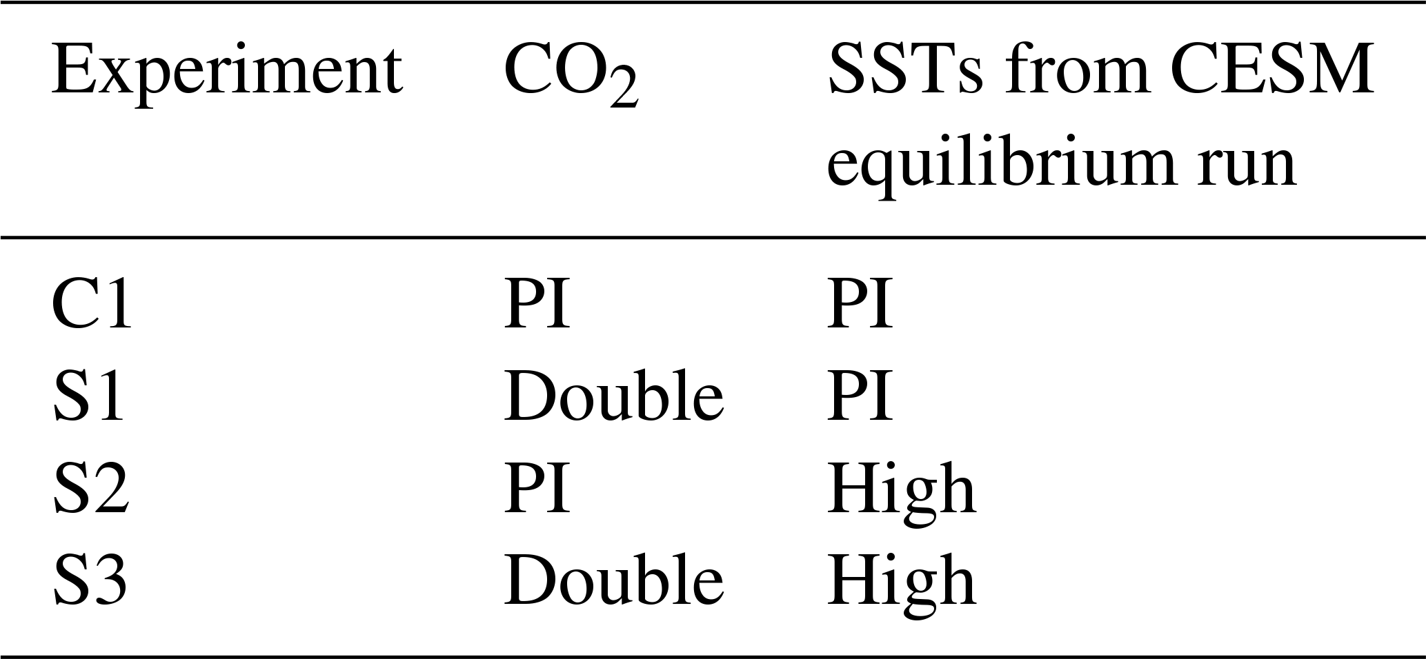
Experiment C1 is the control run with the pre-industrial CO2 concentration (280 parts per million – ppm) and forced with pre-industrial ocean surface conditions, such as sea surface temperatures (SSTs) and sea ice. These SSTs are generated from the Coupled Model Intercomparison Project version 5 (CMIP5) pre-industrial control simulation by the fully coupled Community Earth System Model (CESM). The atmospheric component of CESM is the same as WACCM but does not include stratospheric chemistry (Hurrell et al., 2013). The SSTs might be slightly different when they are generated using a model that also includes atmospheric chemistry; however, this aspect is not considered in this study.
Experiment S1 represents the experiment with the CO2 concentration doubled, as compared to the pre-industrial state (560 ppm), and forced with the same pre-industrial SSTs as in experiment C1. In WACCM, the CO2 concentration does not double everywhere in the atmosphere. Only the surface level CO2 mixing ratio is doubled and, elsewhere in the atmosphere, is calculated according to WACCM's chemical model.
The compset used in this experiment and all the following ones is still F_1850, which means that other radiatively and chemically active gases, such as ozone, will change only because of the changes in the CO2 concentration due to WACCM's interactive chemistry. This also means that the effects of chlorofluorocarbons (CFCs) are not considered in our experiments, as anthropogenic production of CFCs started later than 1850.
In experiment S2, we simulate the scenario in which there is the SSTs forcing from the coupled CESM for the double CO2 condition. This means that the sea surface temperatures are higher than in the PI run, and there is less sea ice. However, in this experiment the CO2 concentration is kept at the pre-industrial value of 280 ppm. S3 represents the experiment with the CO2 concentration in the atmosphere doubled to 560 ppm, and the SSTs are prescribed for the double CO2 climate. Experiments C1, S1, S2 and S3 will be also referred to hereafter in terms of PI, the simulation with high CO2, the simulation with high SSTs and the simulation with high CO2 and SSTs, respectively.
The experimental setup of this study is similar to the setup performed with the Canadian Middle Atmosphere Model (CMAM) by Fomichev et al. (2007) and with the Hamburg Model of the Neutral and Ionized Atmosphere (HAMMONIA) by Schmidt et al. (2006). The HAMMONIA model is coupled to the same chemical model as WACCM–MOZART3. The setup in their study is similar; however, in their study, they double the CO2 concentration from 360 to 720 ppm, while in our study, we double from the pre-industrial level of CO2 (280 ppm).
Note that experiments S2 and S1 are not representing scenarios that could happen in the real atmosphere. These experiments have been used to study the effect of the SSTs separately. Experiment S3 does not take into account other (anthropogenic) changes in the atmosphere not caused by changes in the CO2 concentration and the SSTs.
All the simulations are run for 50 years, of which the last 40 years are used for analysis. In the all results shown, we have used the 40 year mean of our model data.
2.3 Climate feedback response analysis method (CFRAM)
In this study, we aim to quantify the different climate feedbacks that may play a role in the middle atmosphere in a double CO2 climate. For this purpose, we apply the climate feedback response analysis method (CFRAM; Lu and Cai, 2009).
As briefly discussed in the introduction, traditional methods for studying climate feedbacks are based on the energy balance at the top of the atmosphere (TOA). This means that the only climate feedbacks that are taken into consideration are those that affect the radiative balance at the TOA. However, there are other thermodynamic and dynamical processes that do not directly affect the TOA energy balance, while they do yield a temperature response in the atmosphere.
Contrary to TOA-based methods, CFRAM considers all the radiative and non-radiative feedbacks that result from the climate system due to the response to an external forcing. This means that CFRAM starts from a slightly different definition of a feedback process. Note also that, as the changes in temperature are calculated simultaneously, the vertical mean temperature or lapse rate feedback per definition do not exist in CFRAM.
Another advantage of CFRAM is that it allows the measuring of the magnitude of a certain feedback in units of temperature. We can actually calculate how much of the temperature change is due to which process. The climate response aspect in the name of this method refers to the changes in temperature in response to the climate forcings and climate feedbacks.
We refer to the Appendix for the complete formulation of CFRAM diagnostics using outputs of WACCM. Based on the linear decomposition principle, we can solve Eq. (A12) for each of the terms on its right-hand side. This yields the partial temperature changes due to each specific process as follows:
in which R represents the vertical profile of the net long-wave radiation emitted by each layer in the atmosphere and by the surface. S is the vertical profile of the solar radiation absorbed by each layer. The matrix is the Planck feedback matrix, in which the vertical profiles of the changes in the divergence of radiative energy fluxes due to a temperature change are represented. ΔT represents the temperature change.
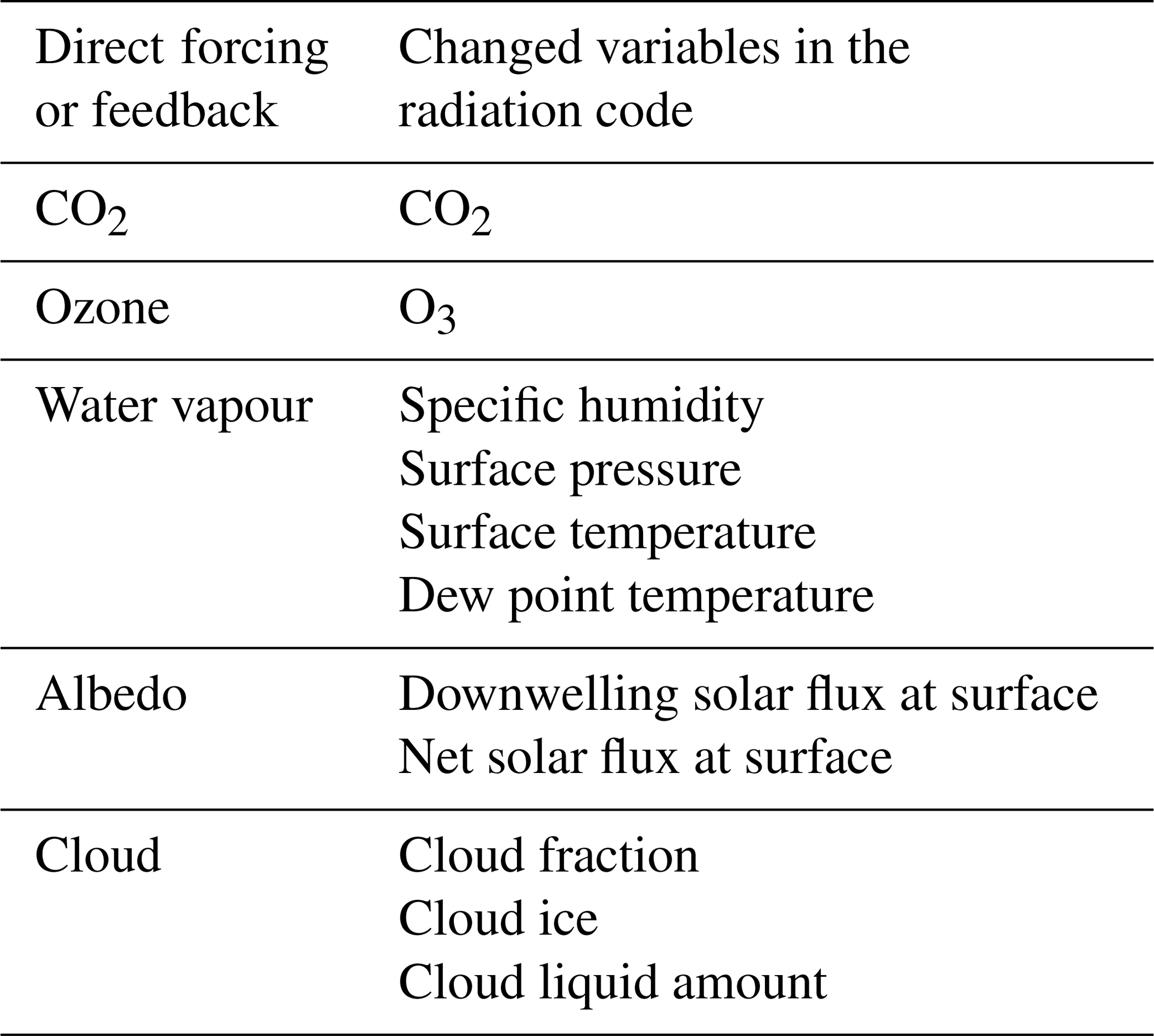
The factors , , Δ(S−R)albedo and Δ(S−R)cloud are calculated by inserting the output variables from WACCM in the radiation code of CFRAM. Here, one takes the output variables from the control run apart from the variable that is related to the direct forcing or the feedback. Table A1 in the Appendix shows which variables from the perturbation runs have been inserted in the radiation code of CFRAM in order to calculate , , Δ(S−R)albedo and Δ(S−R)cloud and, eventually, the associated temperature changes.
Similar to Eqs. (1)–(5), we also calculate the temperature change due to non-local thermal equilibrium (non-LTE) processes and the dynamical feedback. We calculate the terms and Δdyn in Eqs. (A4) and (A7).
The calculated partial temperature changes can be added, with their sum being equal to the total temperature change. It is important to note that this does not mean that the individual processes are physically independent of each other.
The linearization done for Eqs. (A9) and (A10) introduces an error between the temperature difference as calculated by CFRAM and as seen in the model output. Another source of error is that the radiation code of the CFRAM calculations is not exactly equal to the radiation code of WACCM.
For more details on the CFRAM method, please refer to Lu and Cai (2009).
Note that the method used in this study differs from the middle atmosphere climate feedback response analysis method (MCFRAM) used by Zhu et al. 2016). The major difference is that, in this study, we perform the calculations using the units of energy fluxes (Wm−2) instead of converting to heating rates (Ks−1). In other words, we use Wm−2 as the units of heating rates for the layer between two adjacent vertical levels. Because the radiative heating rates are the net radiative energy fluxes entering the layer, it is rather natural and straightforward (i.e. without dividing the mass in the layer to convert it to units of Ks−1) to have the same units of heating rates (convergence) as the radiative energy fluxes. Another difference is that our method is not applicable above 0.01 hPa (∼80 km), while Zhu et al. (2016) added molecular thermal conduction to the energy equation to perform the calculations beyond the mesopause.
As described in Sect. 2.2, four experiments were performed with WACCM, namely a simulation with pre-industrial conditions (experiment C1), a simulation with changed SSTs only (experiment S2), a simulation with only a changed CO2 concentration (experiment S1) and a final simulation with both changed SSTs and CO2 concentration (experiment S3).
Figure 1 shows the zonal mean temperature changes for the different experiments with respect to the pre-industrial state, as modelled by WACCM. The results reach a statistical significance of 95 % for the whole middle atmosphere domain in the experiments S3–C1 and S1–C1 and most of the middle atmosphere for experiment S2–C1. For this figure, and for all the results shown in this paper, we have used the 40 year mean of our data.
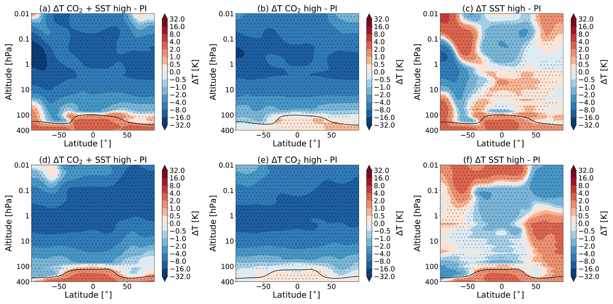
Figure 1The total change in temperature in July (a–c) and January (d–f) for (a, d) the simulation with high CO2 and SSTs (S3), (b, e) the simulation with high CO2 (S1) and (c, f) the simulation with high SSTs (S2), all as compared to the pre-industrial control simulation (C1). The dotted regions indicate the regions where the data reach a confidence level of 95 %. The black line indicates the tropopause height for experiments S3 (a, d), S1 (b, e) and S2 (c, f).
In line with what was shown in earlier studies (e.g. Akmaev, 2006; Fomichev et al., 2007), we observe that an increase in CO2 causes a cooling in the middle atmosphere, with the exception of the cold summer upper mesosphere region. We also observe that changing the SSTs alone, while leaving the CO2 concentration at the pre-industrial levels (Fig. 1c and f), also yields significant temperature changes over a large part of the middle atmosphere and contributes to the observed warming in the cold summer mesopause region.
As found previously by Fomichev et al. (2007) and Schmidt et al. (2006), we find that the sum of the two separate temperature changes in the experiment with changed CO2 only and changed SSTs only (experiments S1 and S2) is approximately equal to the changes observed in the combined simulation (experiment S3). Shepherd (2008) explained that climate change affects the middle atmosphere in two ways: either radiatively, through in situ changes associated with changes in CO2, or dynamically, through changes in stratospheric wave forcing which are primarily a result of changing the SSTs (Shepherd, 2008). Even though the radiative and dynamic processes are not independent, these processes are seen to be approximately additive (Sigmond et al., 2004; Schmidt et al., 2006; Fomichev et al., 2007).
The CFRAM makes it possible to separate and estimate the temperature responses due to an external forcing and various climate feedbacks, such as ozone, water vapour, cloud, albedo and dynamical feedbacks. Note that for the ozone, water vapour, cloud and albedo feedback, we can only calculate the radiative part of the feedback. The response to dynamical changes is calculated in a separate term.
This can be understood as we use the Fu–Liou radiative transfer model (Fu and Liou, 1992, 1993) to do offline calculations of the total local thermal equilibrium (LTE) radiative heating rate perturbation fields between the control experiment (C1) and one of the other three experiments (i.e. S1, or S2 or S3). We use the standard outputs of atmospheric compositions (e.g. CO2 and O3) and thermodynamic fields (e.g. pressure, temperature, water vapour, clouds and surface albedo) and partial LTE radiative heating rate perturbation fields due to perturbations in individual atmospheric composition or thermodynamic fields (e.g. the terms on the right-hand side of Eq. (A9), except the first term).
We use the difference between the offline calculation of the total LTE radiative heating rate perturbations and the original total LTE radiative heating rate perturbations derived directly from the standard WACCM outputs as the error term of our offline LTE radiative heating perturbations. We note that the standard WACCM output fields also include non-LTE radiative heating fields but do not include non-radiative heating rates. Therefore, we use the sum of the total LTE radiative heating rate perturbations and non-LTE radiative heating fields derived from the standard WACCM output fields to infer non-radiative heating rate perturbations under the equilibrium condition, namely Eq. (A8).
We should also note that, because we are using an atmosphere-only model in our experiment, the external forcing is either the change in CO2 concentration or the change in SSTs or both. In an atmosphere–ocean model (such as CESM) and, of course, in reality, the changes in sea surface temperature and sea ice distributions are responses to the changed CO2 concentration.
In Sect. 4.1–4.5, we will discuss the meridional–vertical profiles of the temperature responses to the direct forcing and the various feedbacks during July and January. In Sect. 5, we will discuss regional and global means of partial temperature changes due to feedbacks.
4.1 Direct temperature response to CO2
Figure 2 shows the zonal mean temperature change due to the increase in CO2. We see that increasing CO2 leads to a cooling almost everywhere in the middle atmosphere, except at the high latitudes in the cold summer upper mesosphere where we see a warming instead. The higher the temperature, the more cooling due to the increasing CO2 concentration is found (Shepherd, 2008). The reason for this is that the outgoing long-wave radiation strongly depends on the Planck black-body emission (Zhu et al., 2016).
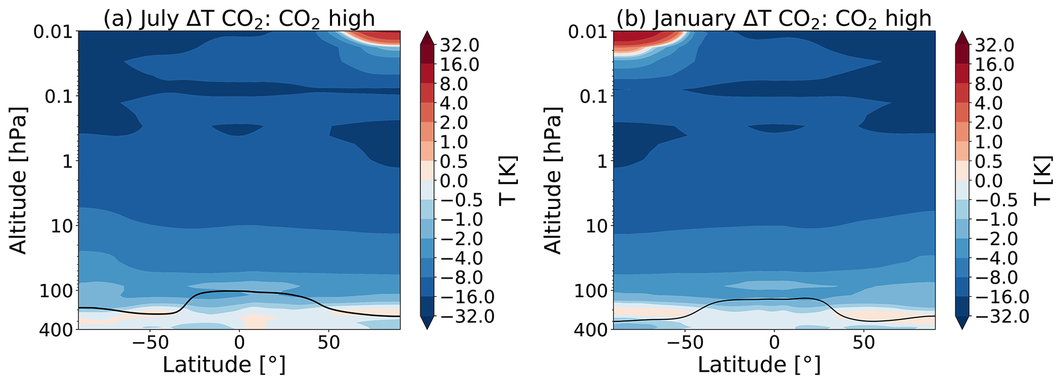
Figure 2Partial temperature change due to the direct forcing of CO2 for July (a) and January (b) due to the doubling of the atmospheric CO2 concentration, as calculated by the climate feedback response analysis method (CFRAM) using experiments S1 and C1. The black line indicates the tropopause height for the S1 run (with a double CO2 concentration).
Changing the SSTs does not lead to a change in CO2 concentration; therefore, the temperature response to changes in CO2 is not present for the run with changed SST only (therefore, we do not show these temperature responses in Fig. 2.).
4.2 Ozone feedback
Ozone plays a crucial role in the chemical and radiative budget of the middle atmosphere. The distribution of ozone in the middle atmosphere is determined by both chemical and dynamical processes. Most of the ozone production takes place in the tropical stratosphere as a result of photochemical processes which involve oxygen. Meridional circulation then transports ozone to other parts of the middle atmosphere (Langematz, 2019). The production of ozone is largely balanced by catalytic destruction cycles involving NOx, HOx and Clx radicals. HOx dominates ozone destruction in the mesosphere and lower stratosphere, while NOx and Clx dominate this process in the middle and upper stratosphere (e.g. Cariolle, 1983).
Since the 1970s, ozone in the middle atmosphere has begun to decline globally due to the increased production of ozone-depleting substances (ODSs) (Brühl and Crutzen, 1988). The Montreal Protocol, adopted in 1987 to stop this threat, eventually led to a slow recovery of the stratospheric ozone over the recent 2 decades (WMO, 2018; Langematz, 2019). In our study, we do not consider the effect of anthropogenic ODSs since pre-industrial times (Langematz, 2019).
In this study, we are interested in the temperature response to changes in ozone concentration induced by the increased CO2 concentration and/or the changes in SST in WACCM. Under enhanced CO2 concentrations, the ratio between O3 and O mixing ratios is generally shifted towards a higher concentration of ozone, which is caused by the strong temperature dependency of the ozone production reaction ().
Figure 3 shows the percentage changes in O3 concentration when the CO2 concentration and/or the SST change. The results reach a statistical significance of 95 % for the whole middle atmosphere domain in the experiments S3–C1 and S1–C1 and most of the middle atmosphere for experiment S2–C1.
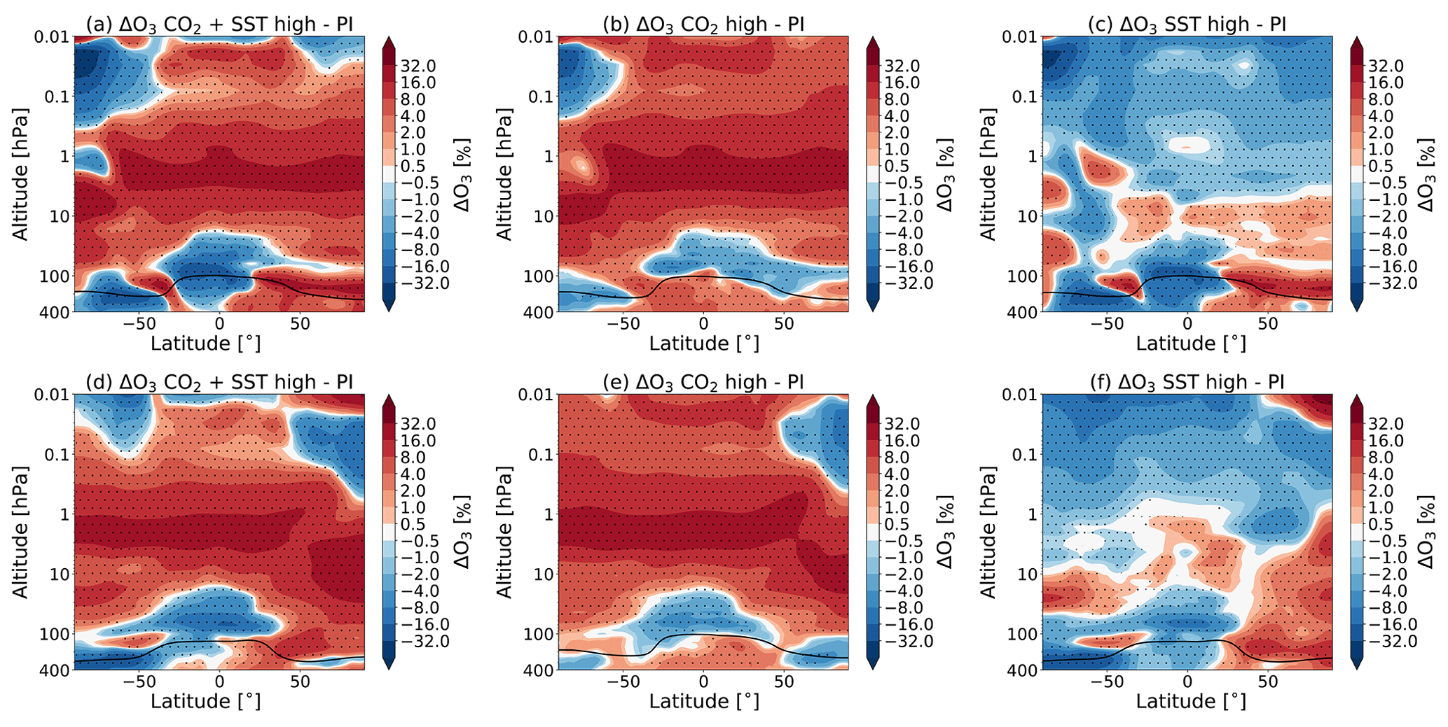
Figure 3The percentage change in the zonal and monthly mean ozone concentration for July (a–c) and January (d–f) due to (a, d) the combined effect of the CO2 increase and SST changes (experiment S3–C1), (b, e) the doubling of the atmospheric CO2 concentration (experiment S1–C1) and the (c, f) SSTs (experiment S2–C1) as simulated by WACCM. The dotted regions indicate the regions where the data reach a confidence level of 95 %. The tropopause height is indicated as in Fig. 1.
We find, as expected, that an increase in CO2 leads to an increase in ozone in most of the middle atmosphere. The increase in O3 is about 20 % around 2 hPa in the tropical region for experiment S3 with respect to C1. This corresponds with what is seen by Fomichev et al., (2007); however, they find that the increase in ozone in January is a bit lower in this region (around 15 %; see their Fig. 7).
There are some regions where the O3 concentration is decreasing. In the tropical lower stratosphere, a decrease of about 20 % is seen; in the summer polar mesosphere (around 0.01 hPa), ozone decreases by 3 %, while in the mesosphere (around 0.02 hPa), ozone decreases by over 30 %. Figure 3c and f show that changing the SSTs also has a significant impact on the ozone concentration. A complete account of the ozone changes is beyond the scope of this paper.
As we will discuss in the next section, an enhanced concentration of CO2 also leads to changes in the dynamics in the middle atmosphere. The stratospheric Brewer–Dobson circulation is projected to strengthen, which would lead to an increase in the poleward transport of ozone. We will also see that an increase in CO2 concentration leads to stronger summer pole to winter pole flow in the mesosphere.
Figure 4 shows the percentage change in the zonal and monthly mean concentration of Cl, NO, O, OH, CH3, NOx and N2O in July due to the combined effect of the CO2 increase and SST changes (experiment S3 vs. C1) as simulated by WACCM. The patterns in January look similar (not shown). These results reach a statistical significance of 95 % for the whole middle atmosphere domain.

Figure 4The percentage change in the zonal and monthly mean concentration of Cl (a), NO (b), O (c), OH (d), CH4 (e), NOx (f) and N2O (g) in July due to the combined effect of the CO2 increase and SST changes (experiment S3 vs. C1) as simulated by WACCM. The dotted regions indicate the regions where the data reach a confidence level of 95 %. The tropopause height is indicated as in Fig. 1.
We would like to point out that the changes in these constituents are only brought about by the CO2 concentration and/or the SSTs. We still use the F_1850 compset, and the only difference between the runs is the forcing in CO2 and SSTs. The changes in chemical constituents look very similar to those found by Schmidt et al. (2006), who performed a similar experiment as discussed in Sect. 2.2 (see their Fig. 20). Note that Fig. 4 shows the changes due to both the CO2 increase and SST changes, while their Fig. 20 shows the percentage changes due to the changes in CO2 concentration only and also only above 1 hPa.
As in Schmidt et al. (2006), we see an decrease in the atomic oxygen (O) mixing ratio at high summer latitudes around 0.01 hPa (see Fig. 4c), which results from increased upwelling. This increase in O leads to a decrease in ozone in this region. We also see a decrease in ozone concentration in the winter polar region around 0.1 hPa (approximately 65 km). This could be caused by an increase in NO and, in a small way, by Cl mixing ratios which result from a stronger subsidence of NO- and Cl-rich air, as suggested in Schmidt et al. (2006). As stated before, a complete discussion of the changes in ozone concentration is beyond the scope of this paper, and the changes in other constituents shown in Fig. 4 are shown for reference only.
What is new in this study is that we can calculate the temperature responses due to the changes in ozone concentration. These temperature responses are shown in Fig. 5. It can be seen that there is a warming in the regions where there is an increase in the O3 concentration, while there is a cooling for the regions with a decrease in the O3 concentration. However, this is not the case for the winter polar region where there is no sunlight. Note that the temperature responses to the changes in CO2 and O3 concentration behave differently in that the temperature responses due to the direct forcing of CO2 follow the temperature distribution quite closely, while the temperature responses due to O3 follow the ozone concentration, as also seen by Zhu et al. (2016).
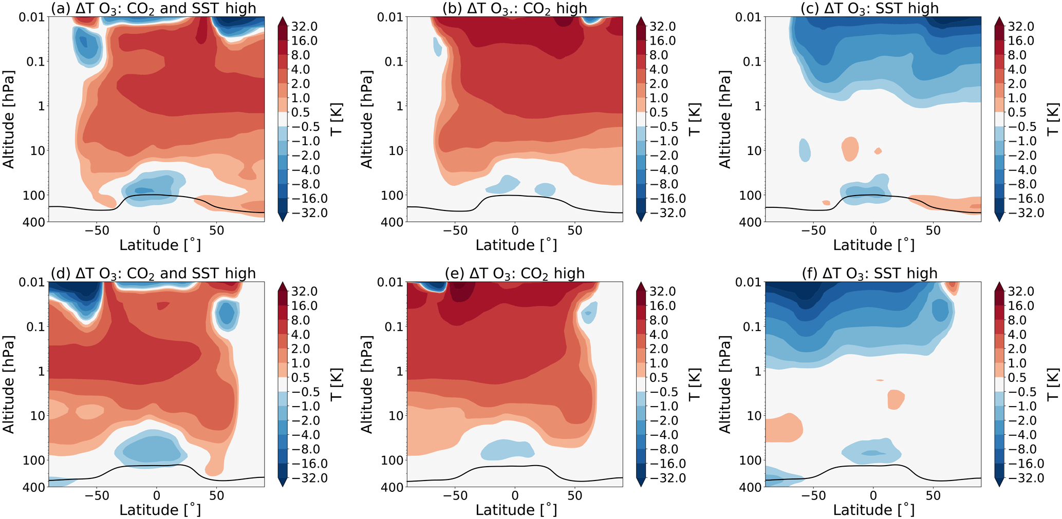
Figure 5Partial temperature responses to changes in O3 concentration, as calculated by CFRAM, in July (a–c) and January (d–f) due to (a, d) the combined effect of the CO2 increase and SST changes (experiment S3), (b, e) the doubling of the atmospheric CO2 concentration (experiment S1) and the (c, f) SSTs (experiment S2). The tropopause height is indicated as in Fig. 1.
4.3 Dynamical feedback
The zonal mean residual circulation forms an important component of the mass transport by the Brewer–Dobson circulation (BDC). It consists of a meridional () and a vertical () component, as defined in the transformed Eulerian mean (TEM) framework. The residual circulation consists of a shallow branch, which controls the transport of air in the tropical lower stratosphere, and a deep branch in the mid-latitude upper stratosphere and mesosphere.
Both of these branches are driven by atmospheric waves. In the winter hemisphere, planetary Rossby waves propagate upwards into the stratosphere where they break and deposit their momentum on the zonal mean flow, which in turn induces a meridional circulation. The two-cell structure in the lower stratosphere, which is present all year round, is driven by synoptic-scale waves. The circulation is also affected by orographic gravity wave drag in the stratosphere and by non-orographic gravity wave drag in the upper mesosphere (Oberländer et al., 2013).
Most climate models show that the BDC and the upwelling in the equatorial region will speed up due to an increase in CO2 concentration (Butchart el al., 2010). It has been shown that the strengthening of the Brewer–Dobson circulation in the lower stratosphere is caused by changes in transient planetary and synoptic-scale waves, while the upper stratospheric changes are due to changes in the propagation properties for gravity waves (Oberländer et al., 2013).
It has been explained that the increased stratospheric resolved wave drag is caused by an increase in the meridional temperature gradient in the stratosphere, which leads to a strengthening of the upper flank of the subtropical jets. This, in turn, shifts the critical layers for Rossby wave breaking upwards, which allows for more Rossby waves to reach the lower stratosphere where they break and deposit their momentum, enhancing the BDC (Shepherd and McLandress, 2011).
The differences in the meridional component of the residual circulation () between the different simulations are shown in Fig. 6. These data are averaged over the 40 years of data. The results reach a statistical significance of 95 % for almost the whole area above 1 hPa for the experiment S1–C1; for the experiment S2–C1, the results reach a statistical significance of 95 % in most of the area below this level. The experiment S3–C1 shows the largest region of statistical significance, apart from some regions below 1 hPa.
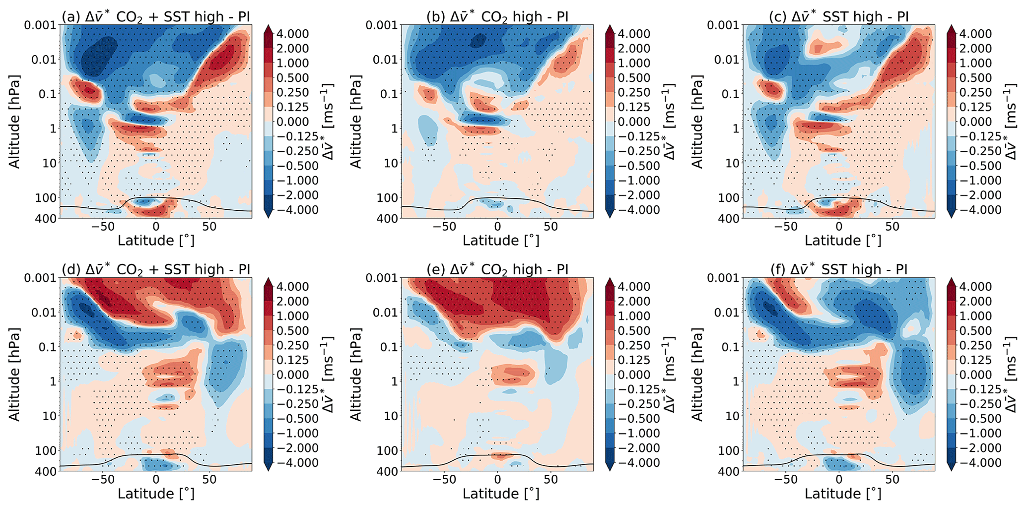
Figure 6Changes in the zonal and monthly mean transformed Eulerian mean residual circulation horizontal velocity for July (a–c) and January (d–f) due to (a, d) the combined effect of the CO2 increase and SST changes (experiment S3–C1), (b, e) the doubling of the atmospheric CO2 concentration (experiment S1–C1) and the (c, f) SSTs (experiment S2–C1) as simulated by WACCM. The dotted regions indicate the regions where the data reach a confidence level of 95 %. The tropopause height is as indicated in Fig. 1.
Figure 6b and e show that only doubling the CO2 concentration leads to a stronger pole to pole flow in the mesosphere. Changing the SSTs also leads to changes in the residual circulation, as can be seen in Fig. 6c and f. Oberländer et al. (2013) showed that the rising CO2 concentration affects the upper stratospheric layers, while the signals in the lower stratosphere are almost completely due to changes in sea surface temperature.
The warmer sea surface temperatures affect the dynamics in the middle atmosphere. It has, for example, been shown that higher SSTs in the tropics lead to an amplification in deep convection, which enhances the generation of quasi-stationary waves (Deckert and Dameris, 2008). Enhanced SSTs lead to an enhanced dissipation of planetary waves and an enhanced dissipation of orographic and non-orographic waves in the upper stratosphere (Oberländer et al., 2013).
We are interested in the temperature responses due to the dynamical feedbacks in the different experiments. These temperature responses are shown in Fig. 7. Figure 7b and e show that there is cooling in the summer mesosphere, while there is warming in the winter mesosphere, which is consistent with a stronger summer to winter pole flow.
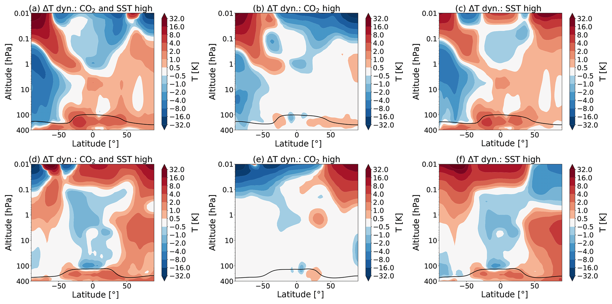
Figure 7Partial temperature responses to changes in dynamics, as calculated by CFRAM, in July (a–c) and January (d–f) due to (a, d) the combined effect of the CO2 increase and SST changes (experiment S3), (b, e) the doubling of the atmospheric CO2 concentration (experiment S1) and the (c, f) SSTs (experiment S2). The tropopause height is indicated as in Fig. 1.
Figure 7c and f show the temperature responses due to changes in the SSTs. It is seen that there is mostly a warming in the summer mesosphere and mostly a cooling in the winter hemisphere, which would weaken the effect of the changed CO2 concentration. Most of the temperature responses in the lower stratosphere are caused by the changes in SSTs, as expected.
In summary, doubling the CO2 concentration leads to a stronger pole to pole flow in the mesosphere, which leads to cooling of the summer mesosphere and a warming of the winter mesosphere. Changing the SSTs weakens this effect but leads to temperature changes in the stratosphere and lower mesosphere.
4.4 Water vapour feedback
Figure 8 shows how the water vapour changes in the middle atmosphere if the CO2 concentration is increased and/or the SSTs are changed with respect to the pre-industrial control run. In WACCM, increasing the CO2 concentration alone leads to a decrease in water vapour in most of the middle atmosphere (Fig. 8b and f). The results reach a statistical significance of 95 % for the whole middle atmosphere domain in the experiments S3–C1 and S2–C1 and most of the middle atmosphere for experiment S1–C1, apart from the winter hemisphere region around 0.1 hPa.
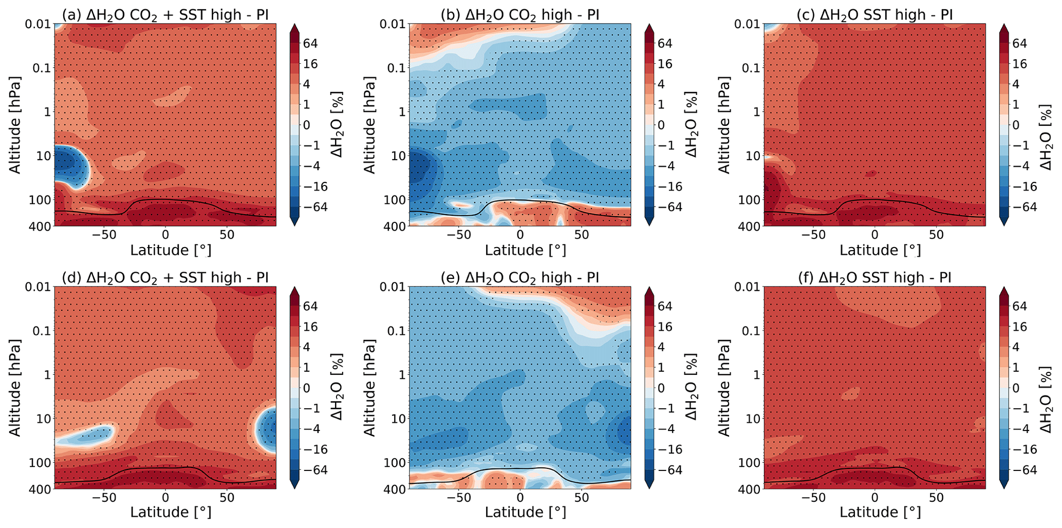
Figure 8The percentage changes in the zonal and monthly mean water vapour mixing ratio for July (a–c) and January (d–f) due to (a, d) the combined effect of the CO2 increase and SST changes (experiment S3–C1), (b, e) the doubling of the atmospheric CO2 concentration (experiment S1–C1) and the (c, f) SSTs (experiment S2–C1), as simulated by WACCM. The dotted regions indicate the regions where the data reach a confidence level of 95 %. The tropopause height is as indicated in Fig. 1.
The amount of water vapour in the stratosphere is determined by transport through the tropopause and by the oxidation of methane in the stratosphere itself. The transport of the water vapour in the stratosphere is mainly a function of the tropopause temperature (Solomon et al., 2010). In WACCM, we see a decrease in temperature in the tropical tropopause for the double CO2 experiment of about −0.25 K. The cold temperatures in the tropical tropopause lead to a reduction in water vapour of between 2 % and 8 % due to freeze-drying in this region.
It can be seen that using the SSTs from the doubled CO2 climate leads to an increase in water vapour almost everywhere in the middle atmosphere, as compared to PI (Fig. 8c and f). In WACCM, forcing with SSTs from a double CO2 climate is shown to lead to a higher and warmer tropopause, which can explain this increase in water vapour. However, it should be noted that models currently have a limited representation of the processes determining the distribution of and variability in lower stratospheric water vapour. Minimum tropopause temperatures are not consistently reproduced by climate models (Solomon et al., 2010; Riese et al., 2012). At the same time, observations are not completely clear about whether there is a persistent positive correlation between the SST and the stratospheric water vapour (Solomon et al., 2010).
Figure 9 shows the temperature responses due to the changes in water vapour, as calculated by CFRAM. It can be seen that, in the regions where there is an increase in the water vapour, there is a cooling and vice versa. This can be understood to mean that increasing the water vapour in the middle atmosphere leads to an increase in long-wave emissions in the mid- and far-infrared by water vapour. This, in turns, leads to a cooling of the region. Similarly, a decrease in water vapour leads to a warming of the region (Brasseur and Solomon, 2005). Figure 8 shows that, above 1 hPa, there is also large percentage changes in water vapour. However, the absolute concentration of water vapour is small there, which explains why there is no temperature response to these changes.
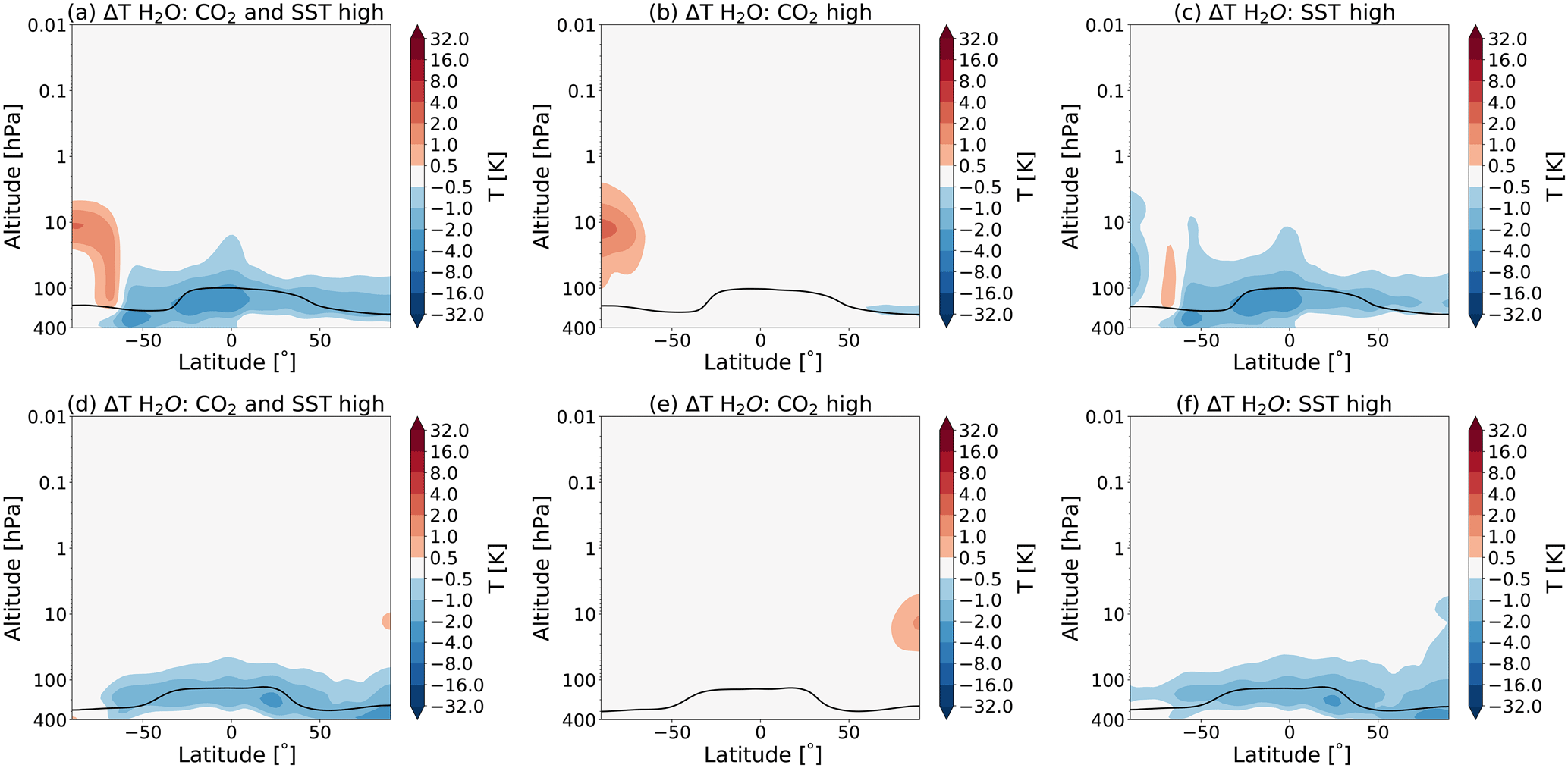
Figure 9Partial temperature responses to changes in water vapour, as calculated by CFRAM, in July (a–c) and January (d–f) due to (a, d) the combined effect of the CO2 increase and SST changes (experiment S3), (b, e) the doubling of the atmospheric CO2 concentration (experiment S1) and the (c, f) SSTs (experiment S2). The tropopause height is indicated as in Fig. 1.
Water vapour plays a secondary, but not negligible, role in determining the middle atmosphere climate sensitivity. In the lower stratosphere, H2O contributes considerably to the cooling in this region. Above 30 hPa, the water vapour contribution to the energy budget is negligible, as also seen in Fomichev et al. (2007).
4.5 Cloud and albedo feedback
Forcing the model with SSTs from the double CO2 climate (as in experiments S2 and S3) yields an overall increase in the cloud cover in the upper troposphere, while this is not the case if one only increases the CO2 concentration (as in experiment S1). Figure 10a and c show the temperature responses to changes in cloud, and Fig. 10b and d show albedo in July and January, respectively, for experiment S2, as calculated by CFRAM.
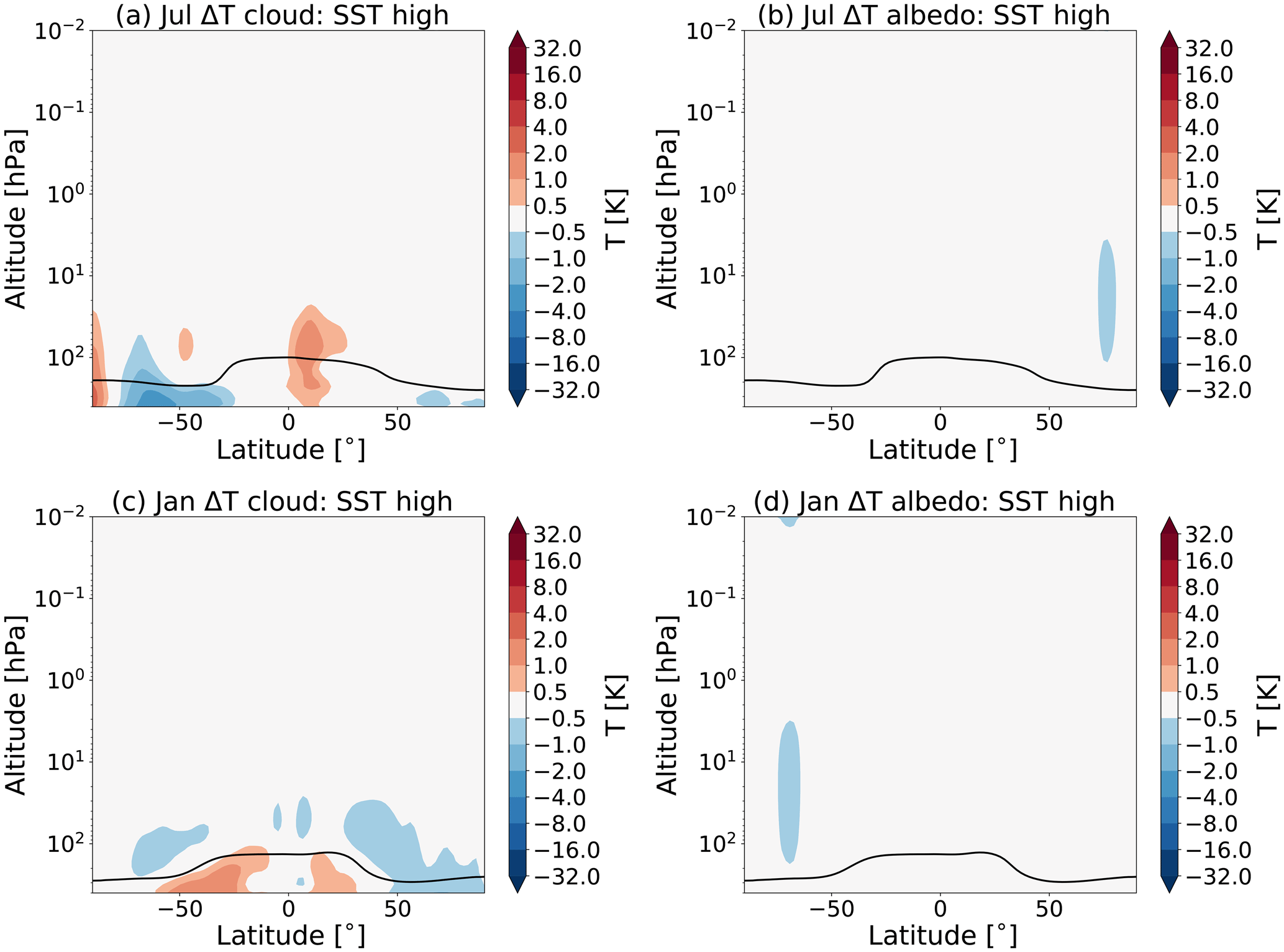
Figure 10Partial temperature responses to changes in clouds (a, c) and albedo (b, d), as calculated by CFRAM, in July (a, b) and January (c, d) due to the SSTs (experiment S2). The tropopause height is indicated as in Fig. 1.
Figure 10 shows that, in the tropical region, there is a warming due to changes in clouds, while there is a cooling at higher latitudes in July (see Fig. 10a). In January, the pattern looks slightly different (see Fig. 10c). These temperature changes are due to changes in the balance between the increased reflected short-wave radiation and the decrease in outgoing long-wave radiation.
We also see an effect of the changes in surface albedo in the stratosphere (see Fig. 10b and d). The cooling in the summer polar stratosphere shown in Fig. 10b and d is due to radiative changes. We suggest that this cooling is due to a decrease in surface albedo, which would lead to less short-wave radiation being reflected. However, more research is needed.
Cloud and albedo feedbacks due to changes in clouds and surface albedo play a crucial role in determining the tropospheric and surface climate (Boucher et al., 2013; Royer et al., 1990). However, it is clear that these feedbacks play only a very small role in the middle atmosphere temperature response to the doubling of CO2 and SSTs.
To study the relative importance of the different feedback processes globally, we show the average change in global mean temperature for the lower stratosphere, the upper stratosphere and the mesosphere for the S3 experiment with the changed CO2 concentration and changed SSTs in Fig. 11. We also show the average change in temperature in the polar regions (90–70 ∘S and 70–90 ∘N) and the tropics (20 ∘S–20 ∘N) for the lower and upper stratosphere and the mesosphere.
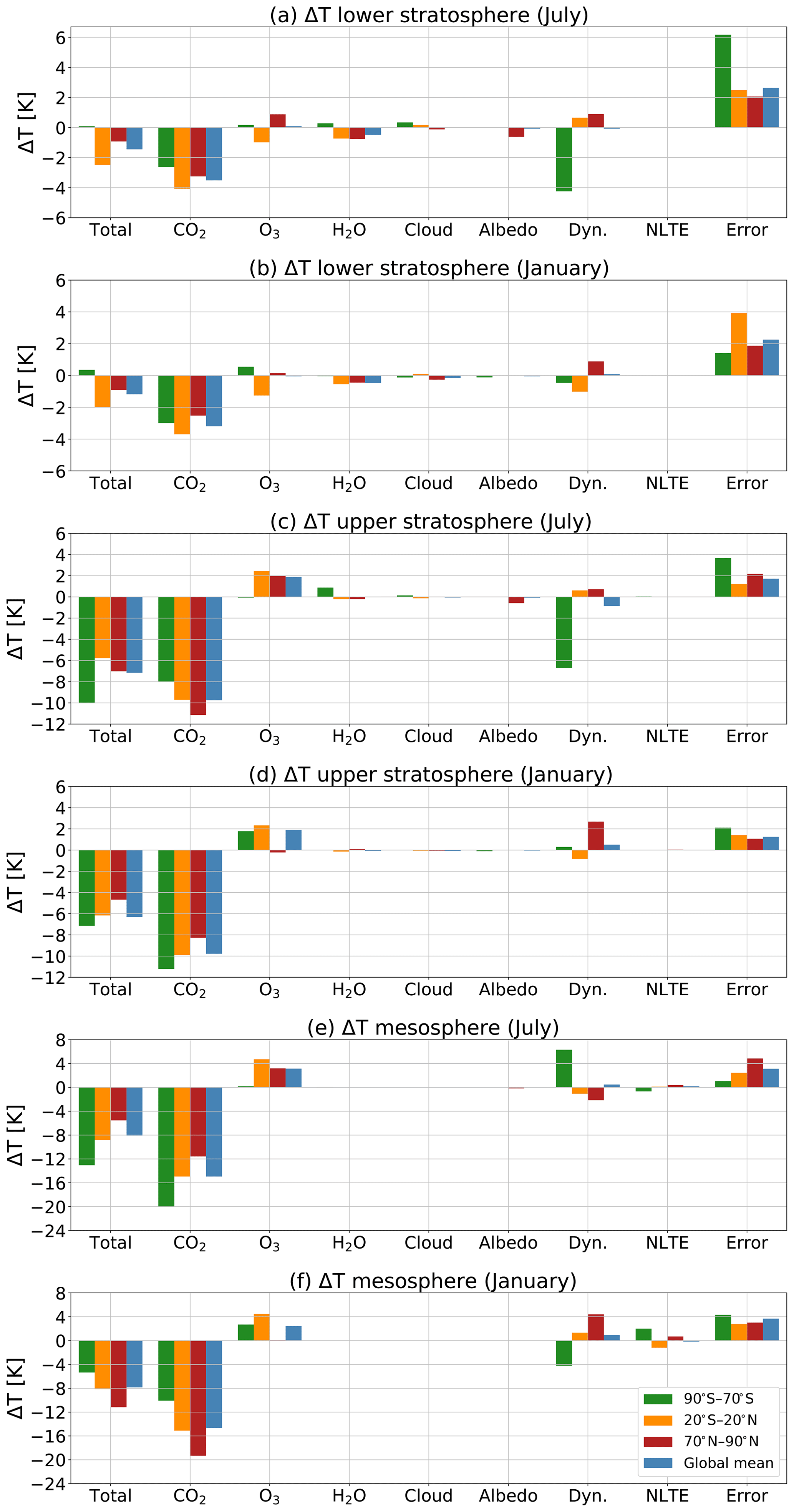
Figure 11The mean temperature responses to the changes in CO2 and various feedback processes in the lower stratosphere from the tropopause height up to 24 hPa (a, b), the upper stratosphere from 24 to 1 hPa (c, d) and in the mesosphere from 1 to 0.01 hPa (e, f) in July (a, c, e) and January (b, d, f) in the polar regions (90–70 ∘S and 70–90 ∘N) and the tropics (20 ∘S–20 ∘N) and the global mean for the S3 experiment (double CO2 and changed SSTs). Note that the range of values on the y axis is not the same for the different subplots.
In order to calculate the lower stratospheric temperature changes, we take the average value of the temperature change from the tropopause up to 24 hPa. The pressure level of the tropopause is simulated in WACCM for each latitude and longitude; we use this pressure level to demarcate between the troposphere and stratosphere. We consider 24 hPa as a crude estimate for the boundary between the lower and upper stratosphere.
The tropopause is not exactly at the same pressure level in the perturbation experiments as compared to the pre-industrial control run (C1). We always take the tropopause of the perturbation experiment which is a bit higher at some latitudes to make sure that we do not use values from the troposphere. We add up the values for each latitude and take the average. This average is not mass weighted. By calculating the average in this way, we can directly compare the vertical values in different regions of the atmosphere. The temperature changes in the upper stratosphere and in the mesosphere are calculated in the same way but then for the altitudes 24–1 hPa and 1–0.01 hPa, respectively.
Figure 11 shows the radiative feedbacks due to ozone, water vapour, clouds, albedo and the dynamical feedback as well as the small contribution due to the non-LTE processes in the NLTE column, as calculated by CFRAM. The “total” column shows the temperature changes in WACCM, while the “error” column shows the difference between temperature changes in WACCM and the sum of the calculated temperature responses in CFRAM. Note that the range of values on the y axis is not the same for the different subplots.
Figure 11 shows that the temperature change in the lower stratosphere due to the direct forcing of CO2 is around 3 K in the global mean. There is a stronger cooling in the tropical region of about 4 K in July and 3.5 K in January. We also observe that there is a cooling of about 1 K due to ozone feedback in the tropical region, while there is a slight warming taking place in the summer hemispheres in both January and July. We also see that the temperature change in the lower stratosphere is influenced by the water vapour feedback. There is a cooling of about 0.5 K in the lower stratosphere, apart from in the southern polar area. There is some small influence from the cloud and albedo feedback, which can be negative or positive (see also Fig. 10).
In the upper stratosphere, the cooling due to the direct forcing of CO2 is, with about 9 K in the global mean, considerably stronger than in the lower stratosphere. The cooling is stronger in the summer polar regions where the cooling due to the direct forcing of CO2 reaches 11 K. In the winter polar region, this cooling is only about 8 K.
The water vapour, cloud and albedo feedback play no role in the upper stratosphere nor in the mesosphere. The ozone feedback results in the positive partial temperature changes in the upper stratosphere, which is about 2 K in the global mean. The changes in ozone do not result in temperature changes in the winter hemisphere, as discussed in Sect. 4.2.
The picture in the mesosphere is similar to that the upper stratosphere. The main difference is that the temperature changes are larger. The global temperature change due to direct forcing of CO2 is about 15 K. The O3 feedback results in a partial temperature changes of about 3 K in the mesosphere in the global mean. The temperature change due to ozone in the equatorial mesosphere is about 4 K, while the warming due to ozone in the summer polar region is a bit smaller at around 3 K. Just like in the upper stratosphere water vapour, cloud and albedo feedback play no role.
We see that the ozone feedback generally yields a radiative feedback that mitigates the cooling, which is due to the direct forcing of CO2. This has been suggested in earlier studies such as Jonsson et al. (2004) and Dietmüller et al. (2014). With CFRAM, it is possible to quantify this effect and to compare it with the effects of other feedbacks in the middle atmosphere. Note that no other method has been able to quantify how much of the temperature change in the middle atmosphere is due to the different feedback processes.
The temperature response due to dynamical feedbacks is small in the global average at less than 1 K. This can be understood as waves generally do not generate momentum and heat but redistribute these instead (Zhu et al., 2016). However, the local responses to dynamical changes in the high latitudes are large, as we have seen in Sect. 4.3. There are some very small temperature responses due to non-LTE effects as well, which mostly contribute to the temperature change in the mesosphere.
The error term is relatively large, as can be seen from the rightmost column in Fig. 11. This term shows the difference between temperature change in WACCM and the sum of the calculated temperature responses in CFRAM (see Eq. 9 in Sect. 2.3). In CFRAM, we assumed that the radiative perturbations can be linearized by neglecting the higher order terms of each thermodynamic feedback and the interactions between these feedbacks; this yields an error.
Cai and Lu (2009) show that this error is larger in the middle atmosphere than for similar calculations in the troposphere. In the middle atmosphere, the density of the atmosphere is smaller, which leads to smaller numerical values of the diagonal elements of the Planck feedback matrix. As a result, the linear solution is very sensitive to forcing in the middle atmosphere. Another part of the error is due to the fact that the radiative transfer model used in the offline CFRAM calculations is different to the radiative transfer model used in the climate simulations with WACCM.
In addition, the vertical profiles of the temperature responses to the direct forcing of CO2 and the feedbacks are shown in Fig. 12. Here, one can see that the increase in CO2 leads to a cooling over almost the whole middle atmosphere; this is an effect that increases with height. We also observe that, in the summer upper mesosphere regions, the increased CO2 concentration leads to a warming. The changes in ozone concentration in response to the doubling of CO2 lead to a warming almost everywhere in the atmosphere. In some places, this warming exceeds 5 K. In the polar winter, the effect of ozone is small due to lack of sunlight.
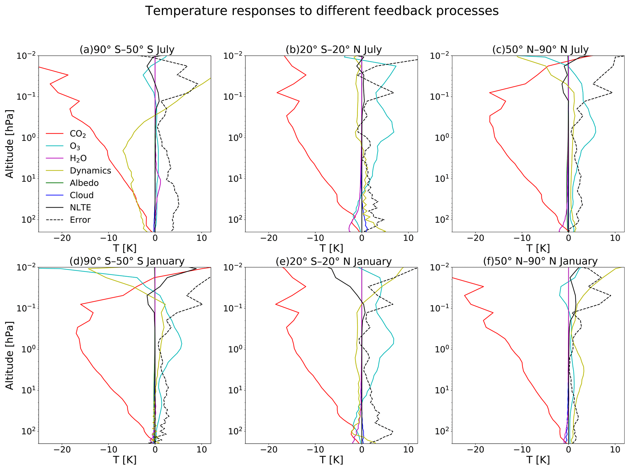
Figure 12Vertical profiles of the temperature responses to the changes in CO2, and various feedback processes in July (a, b, c) and January (d, e, f) due to double CO2 and changed SSTs in the atmosphere between 200 and 0.01 hPa for regions from 50 ∘N and S, both poleward and in the tropics (20 ∘S–20 ∘N), as calculated by CFRAM.
There is also a relatively large temperature response to the changes in dynamics. In Fig. 12, it can be seen that there is a cooling in the summer mesosphere, while there is warming in the winter mesosphere. The water vapour, cloud and albedo feedback play only a very small role in the middle atmosphere, as we observed in Fig. 11. We find that there are also some small temperature changes due to non-LTE effects above 0.1 hPa. How the non-LTE effects exactly cause the small temperature changes in this region is beyond the scope of this paper and needs further investigation.
Figure 13 shows the temperature responses in the upper stratosphere for the experiment with double CO2 (Fig. 13a, b) and changed SSTs (Fig. 13c, d) separately. This has been done to give insight to the temperature response of the CO2 and the SSTs separately. These temperature changes were calculated in the same way as for Fig. 11. Again, the total column shows the temperature changes as simulated by WACCM, the columns CO2, O3, H2O, cloud, albedo, dynamics are shown, and the NLTE column shows the temperature responses due to non-LTE processes as calculated by CFRAM. As in Fig. 11, the error column in Fig. 13 shows the difference between the temperature change in WACCM and the sum of the calculated temperature responses in CFRAM.
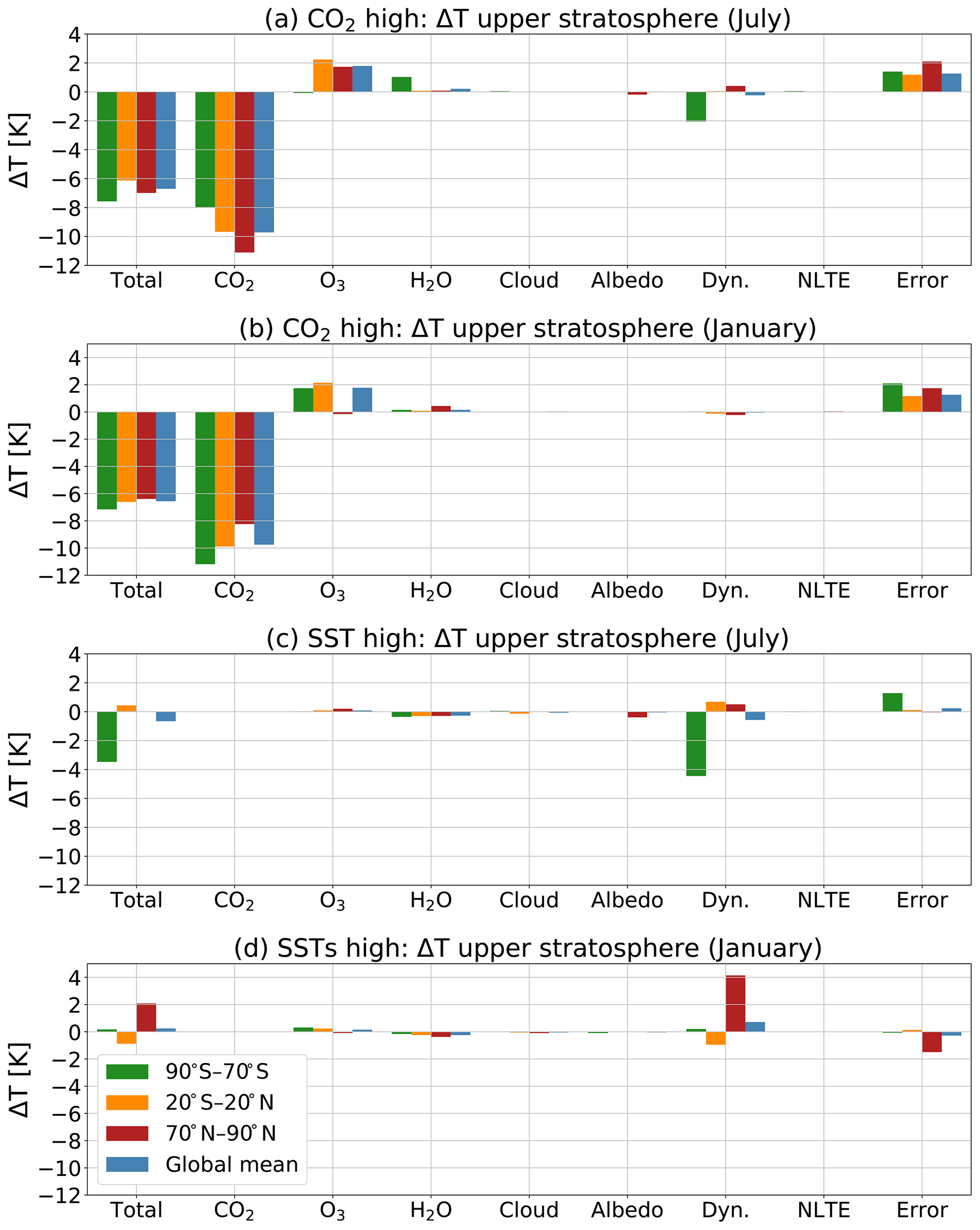
Figure 13The mean temperature responses to the changes in CO2, and various feedback processes in July (a, c) and January (b, d) in the upper stratosphere between 24 and 1 hPa for polar regions (90–70 ∘S and 70–90 ∘N), the tropics (20 ∘S–20 ∘N) and the global mean for the experiment with double CO2 (S1) (a, b) and changed SSTs (S2) separately (c, d).
We learn from this figure that the effects of the changed SSTs on the upper stratosphere are relatively small compared to the effects of changing the CO2. We show the temperature changes for the upper stratosphere as an example. In the lower stratosphere and the mesosphere, we see the same pattern. The effect of the CO2 on the temperature is generally much larger than the effect of the SSTs on the temperature. This finding is consistent with the study of Fomichev et al. (2007), who concluded that the impact of changes in SSTs on the middle atmosphere is relatively small and localized compared to the combined response of changing the CO2 concentration and the SSTs.
The changes in SSTs are, however, responsible for large temperature changes as a result of the dynamical feedbacks, especially in the winter hemispheres where there is a temperature response of 4 K. A similar figure for the lower stratosphere (not shown) shows that the temperature response to the water vapour feedback is almost solely due to changes in the SSTs and not the direct forcing of CO2.
Earlier, we discussed that the sum of the two separate temperature changes in the experiment with double CO2 and changed SSTs is approximately equal to the changes observed in the combined simulation. We find that the same is true for the temperature responses to the different feedback processes.
In this study, we have applied the climate feedback response analysis method to climate sensitivity experiments performed by WACCM. We have examined the middle atmosphere response to CO2 doubling with respect to the pre-industrial state. We investigated the combined effect of doubling CO2 and the subsequent warming SSTs and the effects of separately changing the CO2 and the SSTs. It is important to note that no other method has been able to quantify how much of the temperature change in the middle atmosphere is due to the different feedback processes.
It was found before that the sum of the two separate temperature changes in the experiment with only changed CO2 and only changed SSTs is, at first approximation, equal to the changes observed in the combined simulation (see, for example, Fomichev et al., 2007, and Schmidt et al., 2006). This is also the case for WACCM.
We have found that, even though changing the SSTs yields significant temperature changes over a large part of the middle atmosphere, the effects of the changed SSTs on the middle atmosphere are relatively small compared to the effects of changing the CO2 without changes in the SSTs.
We have given an overview of the mean temperature responses to the changes in CO2 and various feedback processes in the lower stratosphere, upper stratosphere and in the mesosphere in January and July. We find that the temperature change due to the direct forcing of CO2 increases with increasing height in the middle atmosphere. The temperature change in the lower stratosphere due to the direct forcing of CO2 is around 3 K. There is a stronger cooling in the tropical lower stratosphere of about 4 K in July and 3.5 K in January.
In the upper stratosphere, the cooling due to the direct forcing of CO2 is about 9 K, which is considerably stronger than in the lower stratosphere. The cooling is stronger in the summer polar regions, where the cooling reaches a value of 11 K, than in the winter polar region, where the cooling is only about 8 K. In the mesosphere, the cooling due to the direct forcing of CO2 is even stronger at 15 K.
The ozone concentration changes due to changes in the CO2 concentration and by changes in the SSTs. The temperature changes caused by this change in ozone concentration generally mitigate the cooling caused by the direct forcing of CO2. However, in the tropical lower stratosphere and in some regions of the mesosphere, the ozone feedback cools these regions further. In the tropical lower stratosphere, for example, there is a cooling of 1K due to the ozone feedback.
We also have seen that the global mean temperature response due to dynamical feedbacks is small in the global average in all regions at less than 1 K. However, local responses to the changes in dynamics can be large. Doubling the CO2 concentration leads to a stronger summer to winter pole flow, which leads to a cooling of the summer mesosphere and a warming of the winter mesosphere. Changing the SSTs weakens this effect in the mesosphere but affects the temperature response in the stratosphere and lower mesosphere.
Using CFRAM on WACCM data shows that the change in water vapour leads to a cooling of up to 2 K in the lower stratosphere. It should be noted that climate models currently have a limited representation of the processes determining the distribution of and variability in lower stratospheric water vapour. This means that the temperature response to the water vapour feedback might be different when using a different model. We have also seen a small effect of the cloud and albedo feedback on the temperature response in the lower stratosphere, while these feedbacks play no role in the upper stratosphere and the mesosphere.
The results seen in this study are consistent with earlier findings. As in Shepherd (2008), we find that the higher the temperature at a region in the atmosphere, the more cooling there is seen due to the direct feedback of CO2. We find, as in Zhu et al. (2016), that the temperature responses due to the direct forcing of CO2 follow the temperature distribution quite closely, while the temperature responses due to O3 follow the changes in ozone concentration instead.
We have also seen that the ozone feedback generally yields a radiative feedback that mitigates the cooling, which is due to the direct forcing of CO2, and is consistent with earlier studies such as Jonsson et al. (2004) and Dietmüller et al. (2014). CFRAM is the first study that allows the calculation of how much of the temperature response is due to which feedback process.
The next step would be to investigate the exact mechanisms behind the feedback processes in more detail. Some processes can influence the different feedback processes, such as ozone-depleting chemicals influencing the ozone concentration and, thereby, the temperature response of this feedback. A better understanding of the effect of the increased CO2 concentration on the middle atmosphere will help to distinguish the effects of the changes in CO2 and O3 concentration.
There is also a need for a better understanding of how different feedbacks in the middle atmosphere affect the surface climate. As discussed in the introduction, the exact importance of ozone feedback on the global mean temperature is currently not clear (Nowack et al., 2015; Marsh et al., 2016). A similar analysis as, in this paper, can be performed to quantify the effects of feedbacks on the surface climate.
In conclusion, we have seen that CFRAM is an efficient method for quantifying climate feedbacks in the middle atmosphere, although there is a relatively large error due to the linearization in the model. The CFRAM allows the separation and estimation of the temperature responses due to an external forcing and various climate feedbacks such as ozone, water vapour, cloud, albedo and dynamical feedbacks. More research into the exact mechanisms of these feedbacks could help us to better understand the temperature response of the middle atmosphere and their effects on the surface and tropospheric climate.
The mathematical formulation of CFRAM is based on the conservation of total energy (Lu and Cai, 2009). At a given location in the atmosphere, the energy balance in an atmosphere surface column can be written as follows:
R represents the vertical profile of the net long-wave radiation emitted by each layer in the atmosphere and by the surface. S is the vertical profile of the solar radiation absorbed by each layer. Qturb is the convergence of total energy fluxes in each layer due to turbulent motions, and Qconv is the convergence of total energy fluxes into the layers due to convective motion. Dv is the large-scale vertical transport of energy from different layers to others. Dh is the large-scale horizontal transport within the layers, and Wfric is the work done by atmospheric friction. All terms in Eq. (A1) have units of Wm−2.
Due to an external forcing (in this study this is the change in CO2 concentration and/or change in SSTs), the difference in the energy flux terms then becomes the following:
in which the delta (Δ) stands for the difference between the perturbation run and the control run.
CFRAM takes advantage of the fact that the infrared radiation is directly related to the temperatures in the entire column. The temperature changes in the equilibrium response to perturbations in the energy flux terms can be calculated. This is done by requiring that the temperature-induced changes in infrared radiation balance the non-temperature-induced energy flux perturbations.
Equation (A2) can also be written as follows:
The term Δ(S−R) can be calculated as the long-wave heating rate, and the solar heating rate is the output variables of the model simulations. We take the time mean of the WACCM data and perform the calculations for each grid point of the WACCM data. This means that, in the end, we will have the temperature changes at each latitude, longitude and height.
We then calculate the difference in these heating rates for the perturbation simulation and the control simulation.
We use the term Δ(S−R)total to calculate the dynamics term Δdyn.
WACCM provides us with a heating rate in Ks−1. For the CFRAM calculations, we need the energy flux in Wm−2. We can calculate the energy flux by multiplying it with the mass of different layers in the atmosphere and the specific heat capacity.
in which Δ(S−R) is the difference in the short-wave radiation (S) and long-wave radiation (R) between the perturbation run and the control run as a flux in Wm−2, while Δ(S−R)(WACCM) is this difference as the heating rate in Ks−1 in WACCM, with , with p in Pa, cp=1004 J kg−1 K−1 as the specific heat capacity at constant pressure and g the gravitational acceleration 9.81 ms−2.
WACCM includes a non-local thermal equilibrium (non-LTE) radiation scheme above 50 km. It consists of a long-wave radiation (LW) part and a short-wave radiation (SW) part which includes the extreme ultraviolet (EUV) heating rate, chemical potential heating rate, CO2 near-infrared (NIR) heating rate, total auroral heating rate and non-EUV photolysis heating rate.
Therefore, we split the term Δ(S−R)total in an LTE and a non-LTE term as follows:
WACCM provides us with the total long-wave heating rate and the total solar heating rate and the non-LTE long-wave and short-wave heating rates for the different runs. This means that we can calculate the term as well, where we again need to convert our result from Ks−1 to Wm−2 as follows:
This term can be inserted into Eq. (3) as follows:
The central step in CFRAM is to decompose the radiative flux vector using a linear approximation.
We start by decomposing the LTE infrared radiative flux vector ΔR as follows:
where , , , ΔRalbedo and ΔRcloud are the changes in infrared radiative fluxes due to the changes in CO2 ozone, water vapour, albedo and clouds, respectively.
For Eq. (A9), we assumed that radiative perturbations can be linearized by neglecting the higher order terms of each thermodynamic feedback and the interactions between these feedbacks. This is also commonly done in the partial radiative perturbation (PRP) method, in which partial derivatives of the model top of the atmosphere radiation are evaluated with respect to changes in model parameters by a diagnostic rerunning of the model's radiation code (Bony et al., 2006).
The term represents the changes in the infrared (IR) radiative fluxes related to the temperature changes in the entire atmosphere–surface column. The matrix is the Planck feedback matrix in which the vertical profiles of the changes in the divergence of radiative energy fluxes due to a temperature change are represented.
We calculate this feedback matrix using the output variables of the perturbation and the control run of WACCM and inserting the following into the CFRAM radiation code: atmospheric temperature, surface temperature, reference height temperature, ozone, surface pressure, solar insolation, downwelling solar flux at the surface, net solar flux at the surface, dew point temperature, cloud fraction, cloud ice amount, cloud liquid amount, ozone and specific humidity.
Similarly, the changes in the LTE short-wave radiation flux can be written as the sum of the change in short-wave radiation flux due to the direct forcing of CO2 and the different feedbacks, as follows:
Similar to Eq. (A9), we perform a linearization.
Substituting Eqs. (A9) and (A10) into Eq. (A8) yields the following:
This can be written as follows:
As described in the main text of this paper, we can solve Eq. (A12) for each of the terms on its right-hand side based on the linear decomposition principle. This yields the partial temperature changes due to each specific process. The factors , , Δ(S−R)albedo and Δ(S−R)cloud in Eqs. (1–5) are calculated by inserting the output variables from WACCM into the radiation code of CFRAM. Here, one takes the output variables from the control run apart from the variable that is related to the direct forcing or the feedback. The table below shows which variables have been taken from the perturbation runs for each feedback.
Table A1The variables from the perturbation runs inserted in the radiation code of CFRAM to calculate the temperature change in response to the changes in CO2, O3, water vapour, cloud and albedo.
Data sets are available on request to the corresponding author.
MSM ran the WACCM model and the formal analysis and wrote the paper. QZ provided the idea for working with the CFRAM method on WACCM data and supervised the process. MC provided input on the methodology of CFRAM. QW provided the SST data used in the WACCM runs.
The authors declare that they have no conflict of interest.
The computations and simulations were performed on resources provided by the Swedish National Infrastructure for Computing (SNIC) at the National Supercomputer Center (NSC) at Linköping University.
Hamish Struthers (NSC) is acknowledged for his assistance concerning the technical aspects with respect to making the WACCM code run on the NSC supercomputer Tetralith. We thank Qiang Zhang for helping to make the radiation model code applicable to WACCM model data.
This research has been supported by the Swedish Research Council (Vetenskapsrådet; grant nos. 2013-06476 and 2017-04232). The model simulations with WACCM and the data analysis were performed with resources provided by the Swedish National Infrastructure for Computing (SNIC) at the National Supercomputer Centre (NSC), which was partially funded by the Swedish Research Council through grant agreement no. 2016-07213.
The article processing charges for this open-access publication were covered by Stockholm University
This paper was edited by Farahnaz Khosrawi and reviewed by three anonymous referees.
Akmaev, R. A., Fomichev, V. I., and Zhu, X.: Impact of middle-atmospheric composition changes on greenhouse cooling in the upper atmosphere, J. Atmos. Sol.-Terr. Phys, 68, 1879–1889, https://doi.org/10.1016/j.jastp.2006.03.008, 2006.
Beig, G., Keckhut, P., Lower, R. P., Roble, R. G., Mlynczak, M. G., Scheer, J., Fomichev, V. I., Offermann, D., French, W. J. R., Shepherd, M. G., Semenov, A. I., Remsberg, E. E., She, C. Y., Lübken, F. J., Bremer J., Clemensha, B. R., Stegman, J., Sigernes, F., and Fadnavis, S.: Review of mesospheric temperature trends, Rev. Geophys., 41, 4, https://doi.org/10.1029/2002RG000121, 2003.
Bony, S., Colman, R., Kattsov, V. M., Allan, R. P., Bretherton, C. S., Dufresne, J.-L., Hall, A., Hallegatte, S., Holland, M. M., Ingram, W., Randall, D. A., Soden, D. J., Tselioudis, G., and Webb, M. J.: How well do we understand and evaluate climate change feedback processes?, J. Climate, 19, 3445–3482, https://doi.org/10.1175/JCLI3819.1, 2006.
Boucher, O., Randall, D., Artaxo, P., Bretherton, C., Feingold, G., Forster, P., Kerminen, V.-M., Kondo, Y., Liao, H., Lohmann, U., Rasch, P., Satheesh, S. K., Sherwood, S., Stevens, B., and Zhang, X. Y.: Clouds and Aerosols, in: Climate Change: The Physical Science Basis. Contribution of Working Group I to IPCC AR5, edited by: Stocker, T. F., Qin, D., Plattner, G.-K., Tignor, M., Allen, S. K., Boschung, J., Nauels, A., Xia, Y., Bex, V., and Midgley, P. M., Cambridge University Press, Cambridge, United Kingdom and New York, NY, USA, 2013.
Brasseur, G. P. and Solomon, S.: Aeronomy of the middle atmosphere, Chemistry and physics of the stratosphere, Springer, New York, 2005.
Brewer, A. W.: Evidence for a world circulation provided by the measurements of helium and water vapour distribution in the stratosphere, Q. J. Roy. Meteor. Soc., 75, 351–363, https://doi.org/10.1002/qj.49707532603, 1949.
Brühl, C. and Crutzen, P. J.: Scenarios of possible changes in atmospheric temperatures and ozone concentrations due to man's activities, estimated with a one-dimensional coupled photochemical climate model, Clim. Dyn., 2, 173–203, https://doi.org/10.1007/BF01053474, 1988.
Butchart, N, Cionni, I., Eyring, V., Shepherd, T. G., Waugh, D. W., Akiyoshi, H., Austin, J., Brühl, C., Chipperfield, M. P., Cordero, E., Dameris, N., Deckert, R., Dhomse, S., Frith, S. M., Garcia., R. R., Gettelman, A., Giorgetta, M. A., Kinnison, D. E., Li, F., Mancini, E., McLandress, C., Pawson., S., Pirati, G., Plummer, D. A., Rozanov, E., Sassi, F., Scinocca, J. F., Shibata, K., Steil, B., and Tian, W.: Chemistry–climate model simulations of twenty-first century stratospheric climate and circulation changes, J. Climate, 23, 5349–5374, https://doi.org/10.1175/2010JCLI3404.1, 2010.
Caldwell, P. M., Zelinka, M. D., Taylor, K. E., and Marvel, K.: Quantifying the sources of intermodal spread in equilibrium climate sensitivity, J. Climate, 29, 513–524, https://doi.org/10.1175/JCLI-D-15-0352.1, 2016.
Cai, M. and Lu, J.: A new framework for isolating individual feedback processes in coupled general circulation climate models. Part II: Method demonstrations and comparisons, Clim. Dyn., 32, 887–900, https://doi.org/10.1007/s00382-008-0424-4, 2009.
Cariolle, D.: The ozone budget in the stratosphere: Results of a one-dimensional photochemical model, Planet. Space Sci., 31, 1033–1052, https://doi.org/10.1016/0032-0633(83)90093-4, 1983.
Deckert, R. and Dameris, M.: Higher tropical SSTs strengthen the tropical upwelling via deep convection, Geophys. Res. Lett., 35, L10813, https://doi.org/10.1029/2008GL033719, 2008.
Dietmüller, S., Ponater, M., and Sausen, R.: Interactive ozone induces a negative feedback in CO2‐driven climate change simulations. J. Geophys. Res.-Atmos., 119, 1796–1805, https://doi.org/10.1002/2013JD020575, 2014.
Dobson, G. M. B.: Origin and distribution of the polyatomic molecules in the atmosphere, Proc. Math. Phys. Eng. Sci., 236, 187–193, https://doi.org/10.1098/rspa.1956.0127, 1956.
Fomichev, V. I., Jonsson, A. I., De Grandpre, J., Beagley, S. R., McLandress, C., Semeniuk, K., and Shepherd, T. G.: Response of the middle atmosphere to CO2 doubling: Results from the Canadian Middle Atmosphere Model, J. Climate, 20, 1121–1141, https://doi.org/10.1175/JCLI4030.1, 2007.
Fu, Q. and Liou, K. N.: On the correlated k-distribution method for radiative transfer in nonhomogeneous atmospheres, J. Atmos. Sci, 49, 2139–2156, https://doi.org/10.1175/1520-0469(1992)049<2139:OTCDMF>2.0.CO;2, 1992.
Fu, Q. and Liou, K. N.: Parameterization of the radiative properties of cirrus clouds, J. Atmos. Sci, 50, 2008–2025, https://doi.org/10.1175/1520-0469(1993)050<2008:POTRPO>2.0.CO;2 1993.
Hu, X., Y. Li, S. Yang, Y. Deng, and Cai. M.: Process-based decomposition of the decadal climate difference between 2002–13 and 1984–95, J. Climate, 30, 4373–4393, https://doi.org/10.1175/JCLI-D-15-0742.1, 2017.
Hurrell, J. W., Holland, M. M., Gent, P. R., Ghan, S., Kay, J. E., Kushner, P. J., Kamarque, J.-F., Large, W. G., Lawrence, D., Lindsay, K., Lipscomb, W. H., Long, M. C., Mahowald, N., Marsh, D. R., Neale, R. B., Rasch, P., Vavrus, S., Vertenstein, M., Bader, D., Collins, W. D., Hack, J. J., Kiehl, J., and Marchall, S.: The Community Earth System Model: A framework for collaborative research, B. Am. Meteorol., 94, 1339–1360, https://doi.org/10.1175/BAMS-D-12-00121.1, 2013.
Jonsson, A. I., de Grandpré, J., Fomichev, V. I., McConnell, J. C., and Beagley, S. C.: Doubled CO2-induced cooling in the middle atmosphere: Photochemical analysis of the ozone radiative feedback, J. Geophys. Res.-Atmos., 109, D24103, https://doi.org/10.1029/2004JD005093, 2004.
Kinnison, D. E., Brasseur, G. P., Walters, S., Garcia, R. R., Marsh, D. R., Sassi, F., Harvey, V. L., Randall, C. E., Emmons, L., Lamarque, J. F., Hess, P., Orlando, J. J., Tie, X. X., Randall, W., Pan, L. L., Gettelman, A., Granier, C., Diehl, T., Niemeijer, Y., and Simmons, A. J.: Sensitivity of chemical tracers to meteorological parameters in the MOZART-3 chemical transport model, J. Geophys. Res.-Atmos., 112, D20302, https://doi.org/10.1029/2006JD007879, 2007.
Langematz, U.: Stratospheric ozone: down and up through the anthropocene, ChemTexts, 5, 8, https://doi.org/10.1007/s40828-019-0082-7, 2019.
Lindzen, R. S.: Turbulence stress owing to gravity wave and tidal breakdown, J. Geophys. Res.-Oceans, 86, 9707–9714, https://doi.org/10.1029/JC086iC10p09707, 1981.
Lu, J. and Cai, M.: A new framework for isolating individual feedback processes in coupled general circulation climate model. Part I: Formulation, Clim. Dynam, 32, 873–885, https://doi.org/10.1007/s00382-008-0425-3, 2009.
Manabe, S. and Wetherald, R. T.: The effects of doubling the CO2 concentration on the climate of a general circulation model, J. Atmos. Sci, 32, 3–15, 1975.
Marsh, D. R., Mills, M. J. Kinnison, D. E., Lamarque, J. F., Calvo, N., and Polvani, L. M.: Climate change from 1850 to 2005 simulated in CESM1(WACCM), J. Climate, 26, 7372–7391, https://doi.org/10.1175/JCLI-D-12-00558.1, 2013.
Marsh, D. R., Lamarque, J.-F., Conley, A. J., and Polvani, L. M., Stratospheric ozone chemistry feedbacks are not critical for the determination of climate sensitivity in CESM1(WACCM), Geophys. Res. Lett., 43, 3928–3934, https://doi.org/10.1002/2016GL068344, 2016.
McFarlane, N. A.: The effect of orographically excited wave drag on the general circulation of the lower stratosphere and troposphere, J. Atmos. Sci, 44, 1775–1800, https://doi.org/10.1175/1520-0469(1987)044<1775:TEOOEG>2.0.CO;2 , 1987.
Neale, R., Richter, J., Park, S., Lauritzen, P., Vavrus, S., Rasch, P., and Zhang, M: The mean climate of the Community Atmosphere Model (CAM4) in forced SST and fully coupled experiments, J. Climate, 26, 5150–5168, https://doi.org/10.1175/JCLI-D-12-00236.1, 2013.
Nowack, P. J., Abraham, N. L., Maycock, A. C., Braesicke, P., Gregory, J. M., Joshi, M. M., Osprey, A., and Pyle, J. A.: A large ozone-circulation feedback and its implications for global warming assessments, Nat. Clim. Change, 5, 41–45, 2015, https://doi.org/10.1038/NCLIMATE2451, 2015.
Oberländer, S., Langematz, U., and Meul, S.: Unraveling impact factors for future changes in the Brewer-Dobson circulation, J. Geophys. Res.-Atmos., 118, 10296–10312, https://doi.org/10.1002/jgrd.50775, 2013.
Ramaswamy, V., Collins, W., Haywood, J., Lean, J., Mahowald, N., Myhre, G., Naik, V., Shine, K. P., Soden, B., Stenchikov, G., and Storelvmo, T.: Radiative forcing of climate: The historical evolution of the radiative forcing concept, the forcing agents and their quantification, and application, Meteorol. Monogr., 59, 14.1–14.99, https://doi.org/10.1175/AMSMONOGRAPHS-D-19-0001.1, 2019.
Ramaswamy, V., Chanin, M.-L., Angell, J., Barnett, J., Gaffen, D., Gelman, M., Keckhut, P., Koshelhov, Y., Labitzke, K., Lin, J.-J. R., O'Neill, A., Nash, J., Randel, W., Rood, R., Shine, K., Shiotani, M., Swinbank, R.: Stratospheric temperature trends: Observations and model simulations, Rev. Geophys., 39.1, 71–122, https://doi.org/10.1029/1999RG000065, 2001.
Richter, J. H., Sassi, F., and Garcia, R. R.: Toward a physically based gravity wave source parameterization in a general circulation model, J. Atmos. Sci, 67, 136–156, https://doi.org/10.1175/2009JAS3112.1, 2010.
Rieger, V. S., Dietmüller, S., and Ponater, M.: Can feedback analysis be used to uncover the physical origin of climate sensitivity and efficacy differences?, Clim. Dyn., 49, 2831–2844, https://doi.org/10.1007/s00382-016-3476-x, 2017.
Riese, M., Ploeger, F., Rap, A., Vogel, B., Konopka, P., Dameris, M., and Forster, P.: Impact of uncertainties in atmospheric mixing on simulated UTLS composition and related radiative effects, J. Geophys. Res.-Atmos., 117, D16305, https://doi.org/10.1029/2012JD017751, 2012.
Royer, J. F., Planton, S., and Déqué, M.: A sensitivity experiment for the removal of Arctic sea ice with the French spectral general circulation model, Clim. Dyn., 5, 1–17, https://doi.org/10.1007/BF00195850, 1990.
Schmidt, H., Brasseur, G. P, Charron, M., Manzini, E., Giorgetta, M. A., Diehl, T., Fomichev, V., Kinnison, D., Marsh, D., and Walters, S.: The HAMMONIA Chemistry Climate Model: Sensitivity of the mesopause region to the 11-year solar cycle and CO2 doubling, J. Climate, 19, 3903–3931, https://doi.org/10.1175/JCLI3829.1, 2006.
Shaw, T. A. and Shepherd T. G.: Atmospheric science: Raising the roof, Nat. Geosci., 1, 12–13, https://doi.org/10.1038/ngeo.2007.53, 2008.
Shepherd, T. G.: Dynamics, stratospheric ozone and climate change, Atmos. Ocean, 46, 117–138, https://doi.org/10.3137/ao.460106, 2008.
Shepherd, T. G. and McLandress, C.: A robust mechanism for strengthening of the Brewer–Dobson circulation in response to climate change: critical layer control of subtropical wave breaking, J. Atmos. Sci, 68, 784–797, https://doi.org/10.1175/2010JAS3608.1, 2011.
Shine, K. P., Bouqui, M. S., Forster, de F. Forster, P. M., Hare, S. H. E., Langematz, U., Braesicke, P., Grewe, V., Ponater, M., Schnadt, C., Smith, C. A., Haigh, J. D., Austin, J., Butchart, N., Shindell, D. T., Randel, W. J., Nagashima, T., Portmann, R. W., Solomon, S., Seidel, D. J., Lanzante, J., Klein, S., Ramaswamy, V., and Schwarzkopf, M. D.: A comparison of model-simulated trends in stratospheric temperatures, Q. J. Roy. Meteor. Soc. Sci., 129, 1565–1588, https://doi.org/10.1256/qj.02.186, 2003.
Sigmond, M., Siegmund, P. C., Manzini, E., and Kelder, H.: A simulation of the separate climate effects of middle-atmospheric and tropospheric CO2 doubling, J. Climate, 17, 2352–2367, https://doi.org/10.1175/1520-0442(2004)017<2352:ASOTSC>2.0.CO;2, 2004.
Soden, B. and Held, I. M.: An assessment of climate feedbacks in coupled ocean-atmosphere models, J. Climate, 19, 3354–3360, https://doi.org/10.1175/JCLI3799.1, 2006.
Solomon, S., Rosenlof, K. H., Portmann, R. W., Daniel, J. S., Davis, S. M., Sanford, T. J., and Plattner, G. K.: Contributions of stratospheric water vapor to decadal changes in the rate of global warming, Science, 327, 1219–1223, https://doi.org/10.1126/science.1182488, 2010.
Song, X. and Zhang, G. J.: Role of climate feedback in El Niño-like SST response to global warming, J. Climate, 27, 7301–7318, https://doi.org/10.1175/JCLI-D-14-00072.1, 2014.
Taylor, P. C., Cai, M., Hu, A., Meehl, J., Washington, W., and Zhang, G. J.: A decomposition of feedback contributions to polar warming amplification, J. Climate, 26, 7023–7043, https://doi.org/10.1175/JCLI-D-12-00696.1, 2013.
WMO (World Meteorological Organization): Scientific Assessment of Ozone Depletion: 2018, Global Ozone Research and Monitoring Project – Report No. 58, Geneva, Switzerland, 588 pp., available at: https://www.esrl.noaa.gov/csl/assessments/ozone/2018/downloads/2018OzoneAssessment.pdf (last access: 26 October 2020), 2018.
Zhang, P., Wu, Y., Simpson, I. R., Smith, K. L., Zhang, X., De, B., and Callaghan, P.: A stratospheric pathway linking a colder Siberia to Barents-Kara Sea sea ice loss, Sci. Adv., 4, eaat6025, https://doi.org/10.1126/sciadv.aat6025, 2018.
Zheng, J., Zhang, Q., Li, Q., Zhang, Q., and Cai, M.: Contribution of sea ice albedo and insulation effects to Arctic amplification in the EC-Earth Pliocene simulation, Clim. Past, 15, 291–305, https://doi.org/10.5194/cp-15-291-2019, 2019.
Zhu, X., Yee, J.-H., Cai, M., Swartz, W. H., Coy, L., Aquila, V., Garcia, R., and Talaat, E. R.: Diagnosis of middle-atmosphere climate sensitivity by the climate feedback-response analysis method, J. Atmos. Sci., 73, 3–23, https://doi.org/10.1175/JAS-D-15-0013.1, 2016.
- Abstract
- Introduction
- The model and methods
- Temperature responses in a double CO2 scenario
- Meridional–vertical profiles of partial temperature changes
- Regional and global means of partial temperature changes due to feedbacks
- Discussion and conclusions
- Appendix A: Formulation of CFRAM diagnostics using outputs of WACCM
- Data availability
- Author contributions
- Competing interests
- Acknowledgements
- Financial support
- Review statement
- References