Gravitational separation of Ar∕N₂ and age of air in the lowermost stratosphere in airborne observations and a chemical transport model

Accurate simulation of atmospheric circulation, particularly in the lower stratosphere, is challenging due to unresolved wave–mean flow interactions and limited high-resolution observations for validation. Gravity-induced pressure gradients lead to a small but measurable separation of heavy and light gases by molecular diffusion in the stratosphere. Because the relative abundance of Ar to N₂ is exclusively controlled by physical transport, the argon-to-nitrogen ratio (Ar∕N₂) provides an additional constraint on circulation and the age of air (AoA), i.e., the time elapsed since entry of an air parcel into the stratosphere. Here we use airborne measurements of N₂O and Ar∕N₂ from nine campaigns with global coverage spanning 2008–2018 to calculate AoA and to quantify gravitational separation in the lowermost stratosphere. To this end, we develop a new N₂O–AoA relationship using a Markov chain Monte Carlo algorithm. We observe that gravitational separation increases systematically with increasing AoA for samples with AoA between 0 and 3 years. These observations are compared to a simulation of the TOMCAT/SLIMCAT 3-D chemical transport model, which has been updated to include gravitational fractionation of gases. We demonstrate that although AoA at old ages is slightly underestimated in the model, the relationship between Ar∕N₂ and AoA is robust and agrees with the observations. This highlights the potential of Ar∕N₂ to become a new AoA tracer that is subject only to physical transport phenomena and can supplement the suite of available AoA indicators.

1 Introduction

Transport in the middle atmosphere is driven by a combination of advection by the Brewer–Dobson circulation (BDC) (Brewer, 1949; Dobson, 1956) and quasi-horizontal, two-way mixing by breaking waves (Holton et al., 1995). Models consistently predict an acceleration of the BDC due to climate change (Butchart, 2014), but subgrid-scale mixing processes and momentum transfer by unresolved buoyancy waves limit our ability to accurately simulate circulation in the stratosphere (Haynes, 2005; Plumb, 2007). An acceleration of the BDC has important repercussions for stratosphere–troposphere exchange (STE) and thus recovery of the ozone layer and the greenhouse effect of stratospheric water vapor; however, observational evidence of an acceleration of the BDC is weak (Engel et al., 2009, 2017; Waugh, 2009; Ray et al., 2010, 2014).

The mean age of air (AoA) is a widely used indicator of stratospheric circulation (Hall and Plumb, 1994; Waugh and Hall, 2002; Linz et al., 2016). Air can be transported to any location r in the stratosphere via a myriad of different paths, and each path will have an associated transit time. The probability density function that describes the likelihood of air reaching location r with a specific transit time is called the age spectrum. Although the age spectrum is not directly observable, some aspects of its shape can be inferred from observations of short- and long-lived tracers (Andrews et al., 1999, 2001; Schoeberl et al., 2005; Hauck et al., 2019, 2020; Podglajen and Ploeger, 2019). For tracers that are conserved in the stratosphere and whose concentrations increase approximately linearly with time in the troposphere, such as SF₆ and CO₂, the mean AoA, i.e., the first moment of the distribution, can simply be calculated as the time difference, or “lag time”, to when tracer concentrations in the upper troposphere last had comparable values as measured in a stratospheric sample (Hall and Plumb, 1994; Boering et al., 1996; Waugh and Hall, 2002). The stratospheric concentration of N₂O has also been calibrated as an independent AoA tracer by relating the gradual photolytic loss of N₂O in the stratosphere to AoA as determined from CO₂ (Boering et al., 1996; Andrews et al., 2001; Linz et al., 2017).

In contrast to early measurements made on rocket samples (Bieri and Koide, 1970), Ishidoya et al. (2008, 2013) have shown using a balloon-borne sampling system that stratospheric air is detectably fractionated by gravitational settling (GS), with the degree of fractionation strongly correlated to AoA (Ishidoya et al., 2008, 2013, 2018; Sugawara et al., 2018; Belikov et al., 2019). GS leads to depletion of heavier gases in the stratosphere yielding lower ratios of heavy to light gases, e.g., Ar∕N₂, ¹⁸O∕¹⁶O of O₂ and ¹⁵N∕¹⁴N of N₂, with increasing elevation. The vertical gradients induced by gravimetric separation are steeper at higher latitudes (Ishidoya et al., 2008, 2013, 2018; Sugawara et al., 2018), and consistent with patterns observed in stratospheric AoA (Sugawara et al., 2018; Belikov et al., 2019). Gravimetric settling in the stratosphere has also been simulated in 1-D (Keeling, 1988; Ishidoya et al., 2008), 2-D (Ishidoya et al., 2013, 2018; Sugawara et al., 2018), and 3-D stratospheric models (Belikov et al., 2019); 2-D and 3-D models both show a pattern of GS which increases with altitude and latitude, similar to the patterns observed in tracers with a significant stratospheric sink such as N₂O, and consistent with a positive correlation with AoA (Ishidoya et al., 2013; Sugawara et al., 2018; Belikov et al., 2019). Here we attempt to calibrate GS of Ar∕N₂ as an AoA tracer similar to previous work on the N₂O–AoA relationship.

Observing GS in the stratosphere is challenging, however, as the signals are small and because of the need to avoid artifacts caused by temperature- and pressure-induced fractionation near the sampling inlet (Blaine et al., 2006; Ishidoya et al., 2008, 2013). The resulting scatter in existing balloon-based measurements precludes a clear evaluation of the relationship between GS and AoA (Belikov et al., 2019).

Here we present a dataset of gravitational fractionation of Ar∕N₂ and AoA observations made on flask samples from three airborne research projects, totaling nine campaigns in the lowermost stratosphere with mean AoA <3 years (Wofsy et al., 2017, 2018; Stephens, 2017). The HIAPER Pole-to-Pole Observations (HIPPO) project was a global survey of the Pacific troposphere to lower stratosphere on the NSF/NCAR Gulfstream-V aircraft (Wofsy et al., 2011), composed of five individual campaigns from 2008 to 2011. The O₂∕N₂ Ratio and CO₂ Airborne Southern Ocean (ORCAS) study was conducted using the same aircraft but focused on the Drake Passage and Antarctic Peninsula during January–February 2016 (Stephens et al., 2018). The Atmospheric Tomography (ATom) project was a survey of the troposphere and lower stratosphere of the Pacific and Atlantic Ocean basins on the NASA DC-8 aircraft, composed of four individual campaigns from 2016 to 2018 (Prather et al., 2017). The observations are compared to new simulations of GS with the TOMCAT/SLIMCAT (Chipperfield, 2006) tracer transport model. Our goals are to demonstrate the consistency of our data with gravitational fractionation, to evaluate model performance, and to highlight the potential of Ar∕N₂ as a new age tracer.

2 Methods

2.1 Measurements

Discrete 1.5 L flask samples were taken with the NCAR/Scripps Medusa Whole Air Sampler (Bent, 2014; Stephens et al., 2020) (https://www.eol.ucar.edu/instruments/ncar-scripps-airborne-flask-sampler, last access: 7 June 2020). Medusa holds 32 borosilicate glass flasks sealed with Viton o-rings and uses active pressure control to fill the flasks with cryogenically dried air to ∼760 torr. Flasks are shipped to the Scripps Institution of Oceanography (SIO) for analysis of Ar∕N₂ ratios on an IsoPrime Mass Spectrometer. We report changes in Ar∕N₂ ratios in delta notation:

$$\begin{array}{}\text{(1)}& \mathit{\delta }=\left({\displaystyle \frac{R_{\mathrm{SA}}}{R_{\mathrm{REF}}}}-\mathrm{1}\right)\times {\mathrm{10}}^{\mathrm{6}}\left(\mathrm{per}\mathrm{meg}\right),\end{array}$$

where R_SA is the mixing or isotope ratio in the sample and R_REF the ratio in a reference mixture. Measurements are made on the Scripps O2 Program Argon Scale, as defined on 21 January 2020. δ(Ar∕N₂) values are reported after applying an offset to the data to yield a mean of zero in the tropical airborne observations of the free troposphere between 3 and 8 km.

Uncertainty in δ(Ar∕N₂) observations arises from a combination of analytical limitations and artifactual fractionation during sampling. Replicate agreement of surface flasks shows a 1σ repeatability of ±6.1 per meg for δ(Ar∕N₂), but additional scatter in the data may be introduced by small leaks in the Medusa system and thermal or pressure gradient fractionation at the sample intake (Morgan et al., 2020; Stephens et al., 2020). For further details, see Bent (2014). These effects are challenging to separate from true atmospheric variability and differ between campaigns because sampling strategies have generally improved over time. To constrain uncertainty due to aircraft sampling, we quantify total variability in observations from the presumably fairly homogeneous tropical troposphere between 3 and 8 km (Fig. S1 in the Supplement). Data from the earlier campaigns HIPPO 1–5 show a pooled standard deviation of 24 per meg, whereas data from ATom 2–4 yield a pooled standard deviation of 9 per meg, illustrating advances in sampling and sample handling. While no ORCAS samples are available in the tropical troposphere, ORCAS data show similar scatter to ATom 2–4 data between 20 and 50^∘ S. For all campaigns, the uncertainty is small compared to the stratospheric signal of tens to hundreds per meg shown below. We also show that the stratospheric signal in δ(Ar∕N₂) is not due to pressure-dependent inlet fractionation by evaluating the residual δ(Ar∕N₂), which has been corrected for the natural gravitational signal (Fig. S2).

We have compiled available simultaneous, high-frequency measurements of a range of other trace gases, including N₂O, CO₂, O₃, CH₄, and CO, to identify Medusa samples with stratospheric influence and calculate mean AoA. N₂O was measured continuously with a precision of 0.09 ppb at 1 Hz frequency using the Harvard Quantum Cascade Laser Spectrometer (QCLS) (Santoni et al., 2014) during HIPPO and ORCAS and measured every 1–3 min using the NOAA gas chromatograph PAN and Trace Hydrohalocarbon ExpeRiment (PANTHER) during ATom. The Unmanned Aircraft Systems Chromatograph for Atmospheric Trace Species (UCATS) was used to measure O₃ during HIPPO and ATom. O₃ was not measured on ORCAS. We use continuous H₂O data from the NCAR open-path near-infrared multi-pass spectrometer Vertical Cavity Surface Emitting Laser (VCSEL) (Zondlo et al., 2010) for HIPPO and ORCAS, whereas H₂O was measured using the NASA Diode Laser Hygrometer (DLH) (Diskin et al., 2002) during ATom flights. CH₄, CO₂, and CO were measured by QCLS during HIPPO and ORCAS and by the NOAA Picarro (Karion et al., 2013) during ATom. An averaging kernel is applied to the continuous and semi-continuous aircraft data, such as N₂O, O₃, and H₂O, to match it to Medusa samples. The kernel multiplies a weighting function w_i(t) by all continuous data before time t_s, when Medusa switched from sample flask i to sample flask i+1. w_i(t) for each sample i is given by

$$\begin{array}{}\text{(2)}& w_i\left(t\right)=\exp \left[{\displaystyle \frac{-t_{\mathrm{s}}-t}{\mathit{\tau }}}\right],\end{array}$$

where t is each 1 s increment of the continuous data and $\mathit{\tau }=\frac{V}{Q}$ is the flushing time of air in a Medusa flask determined by the flask volume V and airflow Q.

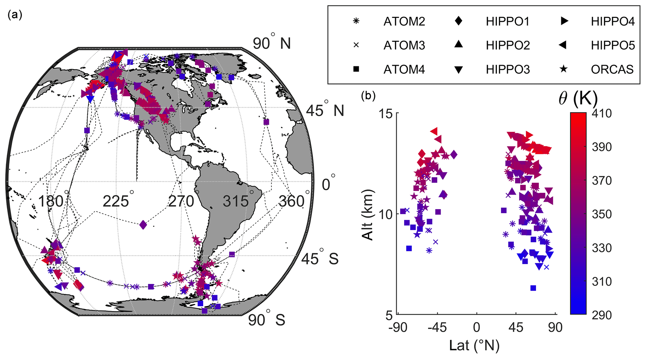
Figure 1 Horizontal (a) and vertical (b) distributions of airborne flask sample locations identified as being of stratospheric origin (see text). Thin dashed black lines on the map illustrate the flight tracks of all nine campaigns. Symbols indicate the campaigns during which the stratospheric samples were collected, and colors show the potential temperature at which the sample was taken.

Stratospheric samples are identified based on their N₂O, O₃, and water vapor levels. Classification based on chemical composition rather than potential temperature or altitude effectively selects samples with a clear stratospheric signature in the lowermost stratosphere and excludes air which has experienced substantial mixing with tropospheric air masses. We label samples as “stratospheric” if (i) water vapor levels are below 15 ppm and either (ii.a) O₃ values exceed 140 ppb or (ii.b) N₂O (detrended to a reference year of 2009) is below 315 ppb. These criteria yield 234 lower stratospheric samples with high-quality N₂O and δ(Ar∕N₂) data, spanning a wide range of latitudes poleward of 40^∘ in both the Northern Hemisphere and Southern Hemisphere (Fig. 1). We use Medusa samples from all five HIPPO campaigns, ORCAS, and ATom 2–4. We do not use samples from ATom 1 because inlet fractionation due to the unique inlet design and location on the DC-8 on this campaign introduced apparent biases on the order of 30 per meg. An additional 25 stratospheric samples are available from the START-08 campaign on the NSF/NCAR GV, but we have not used these here because of the limited number of flasks collected and greater scatter in the data.

2.2 AoA calculation

Stratospheric (mean) AoA for Medusa samples is calculated from N₂O using an updated hemisphere-specific N₂O–AoA relationship. Our method broadly follows Andrews et al. (2001), who assumed a bimodal age spectrum and used multiple observations of CO₂ binned by N₂O values to resolve the seasonal cycle of CO₂ in each bin. Properties of the age spectrum for each N₂O bin, including mean AoA, were constrained by optimizing the agreement between observed CO₂ concentrations and concentrations implied by randomly generated age spectra in each N₂O bin. Andrews et al. (2001) used a highly efficient “genetic algorithm” to yield the most likely relationship between mean AoA and N₂O in each bin. In contrast, we use a more computationally costly Markov chain Monte Carlo (MCMC) method that allows us to obtain more robust uncertainties for all estimated parameters of the age spectrum. Following Malinverno (2002) and Green (1995), our algorithm builds on a Metropolis–Hastings sampler (Metropolis et al., 1953; Hastings, 1970) to evaluate probability distributions for each age spectrum parameter and automatically chooses whether a unimodal or bimodal representation of the age spectrum is more appropriate in each N₂O bin. Finally, we constructed a new tropical upper troposphere reference time series for CO₂ in this study to ensure maximum consistency between all observations used. Analytical and methodological uncertainties are propagated thoroughly and reported as the 95 % confidence interval around a mean.

We consider the tropical upper troposphere to be the single entry point of air into the stratosphere for our AoA calculation. Mixing between tropospheric and lower stratospheric air can occur outside the tropics, leading to air masses that are transitional between stratospheric and tropospheric in the lowermost extratropical stratosphere (e.g., Škerlak et al., 2014). This additional pathway for tropospheric entry has been accounted for in previous studies via additional model information and/or multiple tracers (Ray et al., 1999; Hoor et al., 2004; Bönisch et al., 2009; Hauck et al., 2020). However, we are limited by the number of tracers available to us and therefore instead aim to largely exclude samples influenced through this additional pathway by using thresholds in N₂O, O₃, and H₂O when identifying stratospheric samples. Because of this sample selection strategy, we note that the ages calculated here should not be considered representative of the region that air was sampled in.

Our upper troposphere reference time series (TRTS) consists of a long-term trend and a representation of the mean seasonal cycle. Because direct CO₂ observations in the region are limited, the long-term trend and a first guess of the mean seasonal cycle are estimated from monthly mean surface observations at the Mauna Loa station in Hawaii (MLO, 19^∘ N, 155^∘ W; Fig. 2a) (Keeling et al., 2001) which are later adjusted to match airborne observations in the tropics (20^∘ S–20^∘ N) above 8 km (Fig. 2c). The adjustment includes (i) a constant offset, (ii) a reduced amplitude of the seasonal cycle, and (iii) a phase lag of 1 month. As shown in Fig. 2, after these adjustments the TRTS matches the mean seasonal cycle and absolute value of the airborne data, thus accounting for known vertical gradients of CO₂ and reduced seasonality in the upper troposphere (Fig. 2d). The amplitude of the seasonal cycle in our time series is also in good agreement with the boundary condition used by Andrews et al. (1999, 2001).

Figure 2 Illustration of the major steps in deriving a tropical upper tropospheric reference time series. Panel (a) shows the monthly mean surface CO₂ concentrations at Mauna Loa (MLO) (Keeling et al., 2001) with a stiff spline trend shown in red. Panel (b) shows a fit of the mean seasonal cycle at MLO compared to detrended observations from 1980 to 2019. Panel (c) shows the 1-month lagged seasonal cycle (red line) rescaled in amplitude to match detrended airborne observations in the equatorial upper troposphere (20^∘ S < lat < 20^∘ N, alt >8 km, black). The seasonal cycle derived by Andrews et al. (2001) is presented as a dotted grey line for reference. Panel (d) shows the resulting upper tropospheric mean reference time series (TRTS, red) used for CO₂ in the age-of-air algorithm with the airborne observations from the tropical upper troposphere (black dots) and the time series (grey dotted line) of Andrews et al. (2001).

The new TRTS is used to estimate the age spectrum in 13 N₂O bins of 5 or 10 ppb width (320–325, ..., 290–295, 280–290, ..., 230–240 ppb) using a Markov chain Monte Carlo (MCMC) algorithm which compares observed CO₂ concentrations in the bin to concentration expected from the TRTS. To maximize data availability, we use high-frequency data (see Sect. 2.1) identified as stratospheric according to the criteria above from the 10 s merged products available for HIPPO, ORCAS, and ATom rather than data averaged to the lower Medusa sampling interval for this calibration exercise. Small corrections are applied to the observed CO₂ concentrations (<0.2 ppm) to account for oxidation of CH₄ and CO in the stratosphere.

The MCMC algorithm considers random noise in the TRTS and uses a unimodal or bimodal inverse Gaussian shape of the age spectrum characterized by mean ages Γ₁ and Γ₂ and shape parameters λ₁ and λ₂:

$$\begin{array}{}\text{(3)}& \begin{array}{rl}G& \left(t^{\prime }\mathrm{|}\left({\mathrm{\Gamma }}_{\mathrm{1}},{\mathrm{\Gamma }}_{\mathrm{2}},{\mathit{\lambda }}_{\mathrm{1}},{\mathit{\lambda }}_{\mathrm{2}}\right)\right)=\\ & A\sqrt{{\displaystyle \frac{{\mathit{\lambda }}_{\mathrm{1}}}{\mathrm{2}\mathit{\pi }{t^{\prime }}^{\mathrm{3}}}}}\exp \left(-{\displaystyle \frac{{\mathit{\lambda }}_{\mathrm{1}}{\left(t^{\prime }-{\mathrm{\Gamma }}_{\mathrm{1}}\right)}^{\mathrm{2}}}{\mathrm{2}{\mathrm{\Gamma }}_{\mathrm{1}}^{\mathrm{2}}{t}^{\prime }}}\right)\\ & +(\mathrm{1}-A)\sqrt{{\displaystyle \frac{{\mathit{\lambda }}_{\mathrm{2}}}{\mathrm{2}\mathit{\pi }{t^{\prime }}^{\mathrm{3}}}}}\exp \left(-{\displaystyle \frac{{\mathit{\lambda }}_{\mathrm{2}}{\left(t^{\prime }-{\mathrm{\Gamma }}_{\mathrm{2}}\right)}^{\mathrm{2}}}{\mathrm{2}{\mathrm{\Gamma }}_{\mathrm{2}}^{\mathrm{2}}{t}^{\prime }}}\right),\end{array}\end{array}$$

where factor A determines the relative weight of each peak and a value of A=1 yields a unimodal spectrum (Hall and Plumb, 1994; Andrews et al., 2001; Bönisch et al., 2009). Though more complex representations of the age spectrum have recently been proposed, accounting for multiple modes and seasonal variations (e.g., Bönisch et al., 2009; Li et al., 2012; Hauck et al., 2019, 2020; Podglajen and Ploeger, 2019), these require additional information from multiple tracers or models and good seasonal data coverage that is not available here. In any case, we only rely on the first moment of the age distribution (i.e., the mean age) for calibrating the N₂O–AoA relationship, and the mean age is not particularly sensitive to the assumed shape of the age spectrum (Andrews et al., 2001). By setting A=1 for 50 % of all tested age spectra, the MCMC algorithm automatically selects whether a unimodal or bimodal representation of the age spectrum is optimal for matching observations. Although bimodal solutions with five instead of two free parameters will always be able to fit the data better, a larger number of parameters also decreases the likelihood of randomly selecting a combination of parameters that match the observations well because the fraction of the total parameter space region which yields good agreement with the observation decreases as more parameters are added (Malinverno, 2002). The algorithm is thus able to make an appropriate choice between unimodal and bimodal distributions from the data themselves, without any further a priori assumptions. The MCMC algorithm is set up separately with 2000 independent chains for each N₂O bin to account for uncertainty in the TRTS and obtain best estimates of the mean AoA, i.e., the first moment of Eq. (3). To simplify the algorithm, possible values of ${\mathrm{\Gamma }}_{\mathrm{1}},{\mathrm{\Gamma }}_{\mathrm{2}},{\mathit{\lambda }}_{\mathrm{1}}$, and λ₂ are repeatedly sampled from the same N₂O bin-specific prior distributions. Details of the algorithm are presented in Appendix A.

Finally, the resulting relationship between mean AoA and the N₂O concentration of each bin is fit separately for each hemisphere by a quadratic polynomial, and the polynomial is evaluated at the N₂O value of each Medusa sample to pair every observation of δ(Ar∕N₂) with an AoA. Uncertainty in N₂O and the polynomial fits are propagated by a Monte Carlo scheme. Overall, our method estimates the most likely mean AoA for each Medusa sample and improves upon previous methods by providing a framework for the treatment of uncertainty resulting from (i) analytical error, (ii) uncertainty in the shape of the age spectrum, and (iii) uncertainty in the composition of source gas introduced into the stratosphere.

2.3 TOMCAT/SLIMCAT model

TOMCAT/SLIMCAT (hereafter TOMCAT) is an offline 3-D chemical tracer transport model that has been used extensively for studies of stratospheric ozone depletion and circulation (e.g., Chipperfield, 2006; Chipperfield et al., 2017; Krol et al., 2018). For this study, TOMCAT was run over 31 years, from 1988 to 2018, with a timestep of 30 min at $\mathrm{2.8}{}^{\circ }\times \mathrm{2.8}{}^{\circ }$ horizontal resolution forced by the ERA-Interim reanalysis (Dee et al., 2011) at 60 vertical hybrid sigma-pressure (σ–p) levels up to ∼60–65 km. The first 20 years (i.e., before the first flask observation) were treated as spin-up. The TOMCAT AoA tracer is initialized at the surface and corrected to a value of AoA =0 just below the tropical tropopause. Vertical motion was calculated from the divergence of the horizontal mass fluxes. Although this approach gives slightly younger stratospheric AoA than using isentropic levels and radiative heating rates, it allows a more detailed treatment of tropospheric transport (Chipperfield, 2006; Monge-Sanz et al., 2007). The model simulation was sampled at the times and locations of the Medusa flask observations to provide a direct comparison between the measurements and model.

Following the methodology of Belikov et al. (2019), we include an additional vertical flux term in the model representing the GS of gases in the atmosphere. The vertical flux f_i (mol m⁻² s⁻¹) of tracer i due to molecular diffusion in Earth's gravitational field is given as (Banks and Kockarts, 1973; Belikov et al., 2019)

$$\begin{array}{}\text{(4)}& {\mathit{f}}_i=-D_{i}N{C}_i\left[{\displaystyle \frac{\mathrm{1}}{C_i}}{\displaystyle \frac{\partial C_i}{\partial z}}+\left({\displaystyle \frac{\mathrm{1}}{H_i}}-{\displaystyle \frac{\mathrm{1}}{H_{\mathrm{air}}}}\right)+{\mathit{\alpha }}_i{\displaystyle \frac{\mathrm{1}}{T}}{\displaystyle \frac{\partial T}{\partial z}}\right],\end{array}$$

where D_i is the tracer-specific binary molecular diffusivity in air (m² s⁻¹), N is the number density of air (mol m⁻³), C_i is the mixing ratio, $H_i=\frac{RT}{g{M}_i}$ is the tracer-specific atmospheric equilibrium scale height (m), R is the fundamental gas constant (J K⁻¹ mol⁻¹), g is the gravitational constant (m s⁻²), M_i is the tracer-specific atomic or molecular mass (kg mol⁻¹), α_i is the tracer-specific thermal diffusivity (m² s⁻¹), and T is temperature (K). The three terms in Eq. (4) represent molecular diffusion driven by (i) vertical gradients in the mole fraction of i, (ii) pressure gradients caused by gravity and described by the barometric law, and (iii) temperature gradients (left to right). We neglect the first and third terms in the brackets in Eq. (4), leaving only the gravitational settling term $\left(\frac{\mathrm{1}}{H_i}-\frac{\mathrm{1}}{H_{\mathrm{air}}}\right)$ on the basis that both terms are orders of magnitude less important than the gravitational separation term under stratospheric conditions (see Appendix B) (Ishidoya et al., 2013; Belikov et al., 2019). No fluxes are allowed through the top boundary, and C_i is held constant at the Earth's surface.

To simplify the numerical treatment, we simulate an idealized reference tracer of gravitational fractionation δ_GST, which has a molecular mass 1 amu greater than air and diffusivity equal to that of Ar (see Appendices B and C). This tracer can be scaled offline to obtain the gravitational separation signal in any other species, including δ(Ar∕N₂), e.g.,

$$\begin{array}{}\text{(5)}& \begin{array}{rl}\mathit{\delta }& \left(\mathrm{Ar}/{\mathrm{N}}_{\mathrm{2}}\right)\approx \\ & {\displaystyle \frac{\left(M_{\mathrm{Ar}}-M_{\mathrm{air}}\right)\times D_{\mathrm{Ar}}-\left(M_{{\mathrm{N}}_{\mathrm{2}}}-M_{\mathrm{air}}\right)\times D_{{\mathrm{N}}_{\mathrm{2}}}}{\left(M_{\mathrm{GST}}-M_{\mathrm{air}}\right)\times D_{\mathrm{GST}}}}\times {\mathit{\delta }}_{\mathrm{GST}}.\end{array}\end{array}$$

The appropriate diffusivity values D_Ar and $D_{{\mathrm{N}}_{\mathrm{2}}}$ for Ar and N₂ in air are derived in Appendix B for a ternary mixture of Ar, O₂, and N₂, extending previous work (Ishidoya et al., 2013; Belikov et al., 2019). δ_GST is divided by D_GST in Eq. (5) and therefore does not depend on the exact value chosen for D_GST.

2.4 NIES TM model

We compare our results to previous simulations of GS using the National Institute for Environmental Studies chemical transport model (NIES TM) published recently by Belikov et al. (2019). The NIES TM is a 3-D transport model of similar complexity to TOMCAT driven by the Japanese 25-year Reanalysis (JRA-25) with a hybrid sigma–isentropic (σ–θ) vertical coordinate up to 5 hPa or ∼35 km. The model and GS results are described in detail in Belikov et al. (2013, 2019), respectively.

3 Results

3.1 N₂O–AoA calibration

Our new relationships between N₂O and mean AoA for the Northern Hemisphere and Southern Hemisphere (NH and SH) are well constrained by the observations and generally follow the mid-latitude NH calibration curve of Andrews et al. (2001) (Fig. 3d). At mean AoA >2.5, the N₂O–AoA relationship yields slightly younger ages in the NH than in the SH and compared to the previously published curve, suggesting there might be a latitudinal dependence of the relationship. Such a latitude dependence is, in fact, expected based on theory (Plumb, 2007). We expect curvature and a latitudinal difference in the N₂O–AoA relationship because photolysis of N₂O depends on latitude and altitude due to local sunlight availability. Furthermore, mixing of young and old air results in a mixture with an anomalously low N₂O concentration for a given age. Since the SH, NH, and tropics feature different photolysis rates and show different degrees of mixing/isolation, different N₂O–AoA relationships are expected.

Figure 3 Hemisphere-specific properties of the age spectra in different N₂O bins from the 10 s averaged airborne observations estimated by Markov chain Monte Carlo. Panels (a)–(c) show the value and 95 % confidence interval of Γ₁ Γ₂ and A in each bin for either a unimodal (blue and red circles) or bimodal (faint blue and faint red stars) age spectrum depending on which type was preferentially selected by the algorithm. N₂O values are offset by 1.4 ppb for all Northern Hemisphere estimates (NH, red) for visual clarity in panels (a)–(c). Panel (d) shows the mean AoA and confidence interval of the age spectra ensemble in each bin (i.e., unimodal and bimodal together). These data are fit by a quadratic polynomial for each hemisphere with a fixed y intercept (NH AoA $=-\mathrm{0.0002381}(\mathrm{323.23}-{\mathrm{N}}_{\mathrm{2}}\mathrm{O}{)}^{\mathrm{2}}+\mathrm{0.05567}(\mathrm{323.23}-{\mathrm{N}}_{\mathrm{2}}\mathrm{O})$; SH AoA $=-\mathrm{0.0001723}(\mathrm{323.23}-{\mathrm{N}}_{\mathrm{2}}\mathrm{O}{)}^{\mathrm{2}}+\mathrm{0.05317}(\mathrm{323.23}-{\mathrm{N}}_{\mathrm{2}}\mathrm{O})$). Previous relationships published by Andrews et al. (2001) and Strahan et al. (2011) are given as a dashed and dotted line for reference. y-intercept values of the previously published N₂O–AoA calibrations have been updated to reflect the gradual increase in tropospheric N₂O between 1997 and the new reference year 2009.

Unimodal age spectra are generally preferentially selected by the algorithm, in particular for the SH (Fig. 3a–c), but unimodal age spectra dominate the solution ensemble by a small margin except for AoA <0.5 years (Fig. S3). Confidence intervals on age spectra parameters from bimodal spectra are considerably wider than for unimodal spectra. This implies that the parameters in a bimodal distribution are redundant and the shape of the age spectrum is not sufficiently constrained by the observations used. The width of the spectrum in each N₂O bin varies widely within the prescribed bounds for most unimodal and bimodal age spectra (Fig. S3). It appears that not enough data are available from the airborne campaigns to determine the amplitude of the seasonal cycle with enough confidence to constrain the width of the age spectrum and distinguish the relative contribution of the old peak (influencing primarily the mean concentration difference to the troposphere) and the young peak (controlling the amplitude of seasonality) in bimodal age spectra. Additional observations with less scatter or information from different age tracers are needed to properly resolve the shape of the age spectra. Despite the limited resolution of the seasonal cycle, the observations are sufficient to place tight limits on the mean AoA in each N₂O bin and yield a well-characterized relationship between N₂O and mean AoA for each hemisphere.

3.2 The relationship between mean AoA and GS in models and observations

A comparison of the AoA–GS relationship with observations yields good agreement for the TOMCAT model results within the observational uncertainties (Fig. 4a), but the observations fall outside the range of GS predicted by the NIES TM (Belikov et al., 2019) for mean AoA >1 year (Fig. 4b). For young samples with mean AoA <3 years, GS of δ(Ar∕N₂) increases by roughly 35–45 per meg per year of AoA in both TOMCAT and observations and converges to zero for the youngest samples. In the upper stratosphere, TOMCAT does not obtain any ages as old as observed by Ishidoya et al. (2008, 2013, 2018) and therefore cannot reproduce these observations directly. Changing the vertical coordinate system of TOMCAT or forcing the model with a different reanalysis product could improve agreement with the observations for old ages because TOMCAT in the configuration used here is known to slightly underestimate AoA in the upper stratosphere (Monge-Sanz et al., 2007; Chabrillat et al., 2018). The very steep AoA–GS relationship for the oldest simulated air is however seen in TOMCAT and the balloon observations.

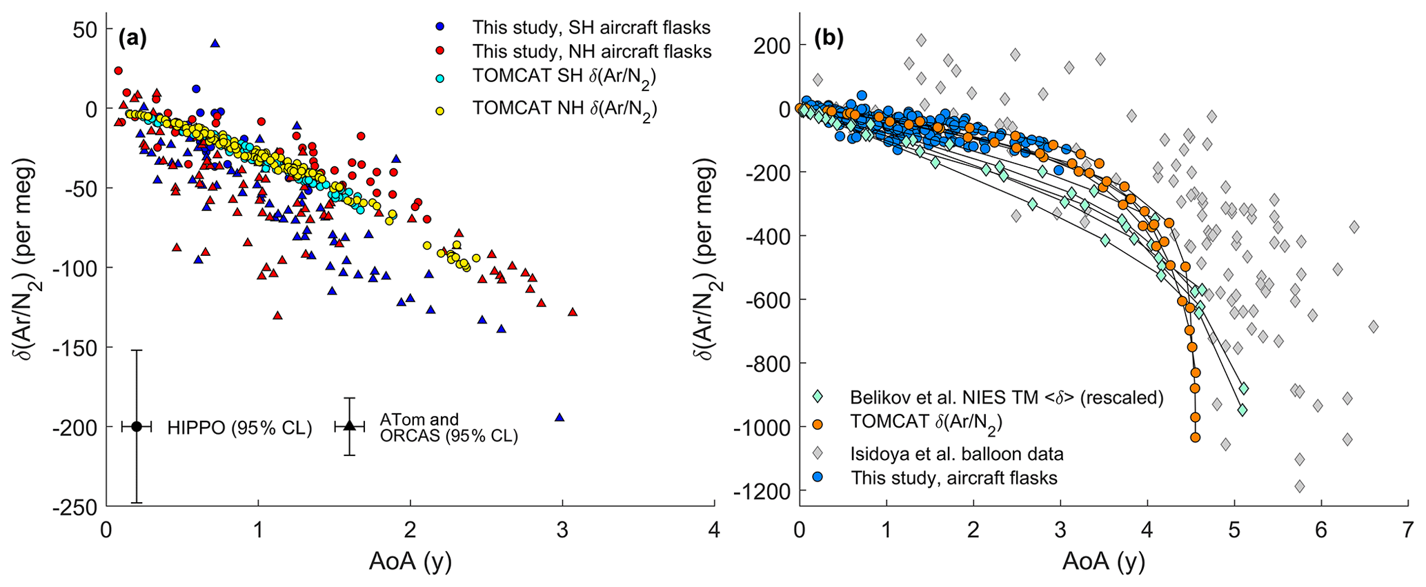
Figure 4 Comparison of age of air (AoA) and gravitational settling (GS) of δ(Ar∕N₂) in models and observations. Panel (a) shows observations from the Northern Hemisphere (red) and Southern Hemisphere (blue) together with TOMCAT model output (SH: cyan; NH: yellow) selected from the closest model grid box in time and space. Because uncertainty for AoA is similar for all stratospheric samples but δ(Ar∕N₂) uncertainty differs between campaigns, representative error bars (95 % confidence interval) are shown for HIPPO (triangles) and ATom/ORCAS (circles) at an arbitrary AoA. δ(Ar∕N₂) is normalized to yield a delta value of zero in the equatorial free troposphere. In panel (b), observations from airborne campaigns (this study) and the balloon sampling system (Ishidoya et al., 2008, 2013, 2018; Sugawara et al., 2018) are plotted with the AoA–GS relationship observed in TOMCAT and the NIES TM (Belikov et al., 2019) as lines for each of the latitude bands shown in Fig. 5 and points for different altitude bins between 10 and 35 km. To yield an equivalent estimate of δ(Ar∕N₂), δ(¹³CO₂∕¹²CO₂) results from the NIES TM (Belikov et al., 2019) have been rescaled according to Eq. (5) and offset by ∼10 per meg to account for the different tropospheric reference region in the definition of δ.

A comparison of δ(Ar∕N₂) and AoA between flask samples and TOMCAT is shown in Fig. S4. However, the direct comparison should not be considered a good test of model performance because our stratospheric composition criteria intentionally target unusually old air in the lowermost stratosphere. For the same reason, profiles of δ(Ar∕N₂) and AoA are not evaluated here. Instead, we suggest the AoA–GS relationship provides a more robust metric for comparison. Overall, our observations validate the implementation of GS for young (<3 years) ages in TOMCAT.

The relationship between mean AoA and GS differs between TOMCAT and the NIES TM (Fig. 5). The NIES TM shows weaker curvature in the relationship overall and produces larger declines in Ar∕N₂ at ages less than 4.5 years compared to TOMCAT. In TOMCAT's mesosphere (which is at the limit of the domain covered by the ERA-Interim reanalyses forcing the model), AoA is near uniform, but GS continues to increase with increasing altitude, changing the relationship between mean AoA and GS in this region. The AoA–GS relationship in TOMCAT is very similar in all non-tropical regions (outside 15^∘ > lat $>-\mathrm{15}$^∘), whereas the curvature of the relationship is slightly stronger in the tropics. In contrast, the NIES TM has a clear dependence of the AoA–GS relationship on latitude. There is also some evidence in the observations of a dependence of the AoA–GS relationship on hemisphere. In the observations, δ(Ar∕N₂) values appear to be slightly more negative in the SH than in the NH for the same age, particularly for AoA >1.5 years. However, almost all SH samples with mean AoA older than 1.5 years come only from the ORCAS campaign. This campaign used a different inlet design than HIPPO and ATom, which could cause a small artifactual offset, but the scatter in our observations generally makes it difficult to separate signal from noise for small interhemispheric differences.

Figure 5 Comparison of the annual and zonal mean age of air (AoA) relationship with gravitational settling simulated in TOMCAT and the NIES TM. The relationship is plotted as lines for the latitude bands indicated by marker color. For the NIES TM, markers show the vertical profile using all grid boxes available between ∼10 and 35 km. For TOMCAT, markers instead correspond to binned altitude bands between 10 and 35 km with a spacing of 2.5 km because of the finer vertical resolution of the model. To yield an equivalent estimate of δ(Ar∕N₂), δ(¹³CO₂∕¹²CO₂) results from the NIES TM (Belikov et al., 2019) have been rescaled according to Eq. (5) and offset by ∼10 per meg to account for the different tropospheric reference region in the definition of δ.

3.3 GS and AoA in TOMCAT

Annual mean δ(Ar∕N₂) in TOMCAT follows the typical pattern of a tracer with a stratospheric sink (Chipperfield, 2006), as previously found in simulations using the NIES TM (Belikov et al., 2019) and the SOCRATES model (Ishidoya et al., 2013; Sugawara et al., 2018) (Fig. 6). δ(Ar∕N₂) is zero in the troposphere and decreases with elevation. The most depleted δ(Ar∕N₂) is observed at high latitudes where sinking air of the Brewer–Dobson circulation advects strongly fractionated air downward. In the tropics, δ(Ar∕N₂) values are considerably less fractionated at the same altitude due to upwelling of unfractionated tropospheric air. Vertical gradients in δ(Ar∕N₂) generally increase with altitude and are largest in the mesosphere (>50 km) because molecular diffusion increases with decreasing pressure and eventually dominates above the turbopause (not shown). There are strong seasonal changes in δ(Ar∕N₂) depletion on the order of several thousand per meg, in particular in the high-latitude mesosphere, with the strongest fractionation occurring during the winter season (see movie available with online version of the paper).

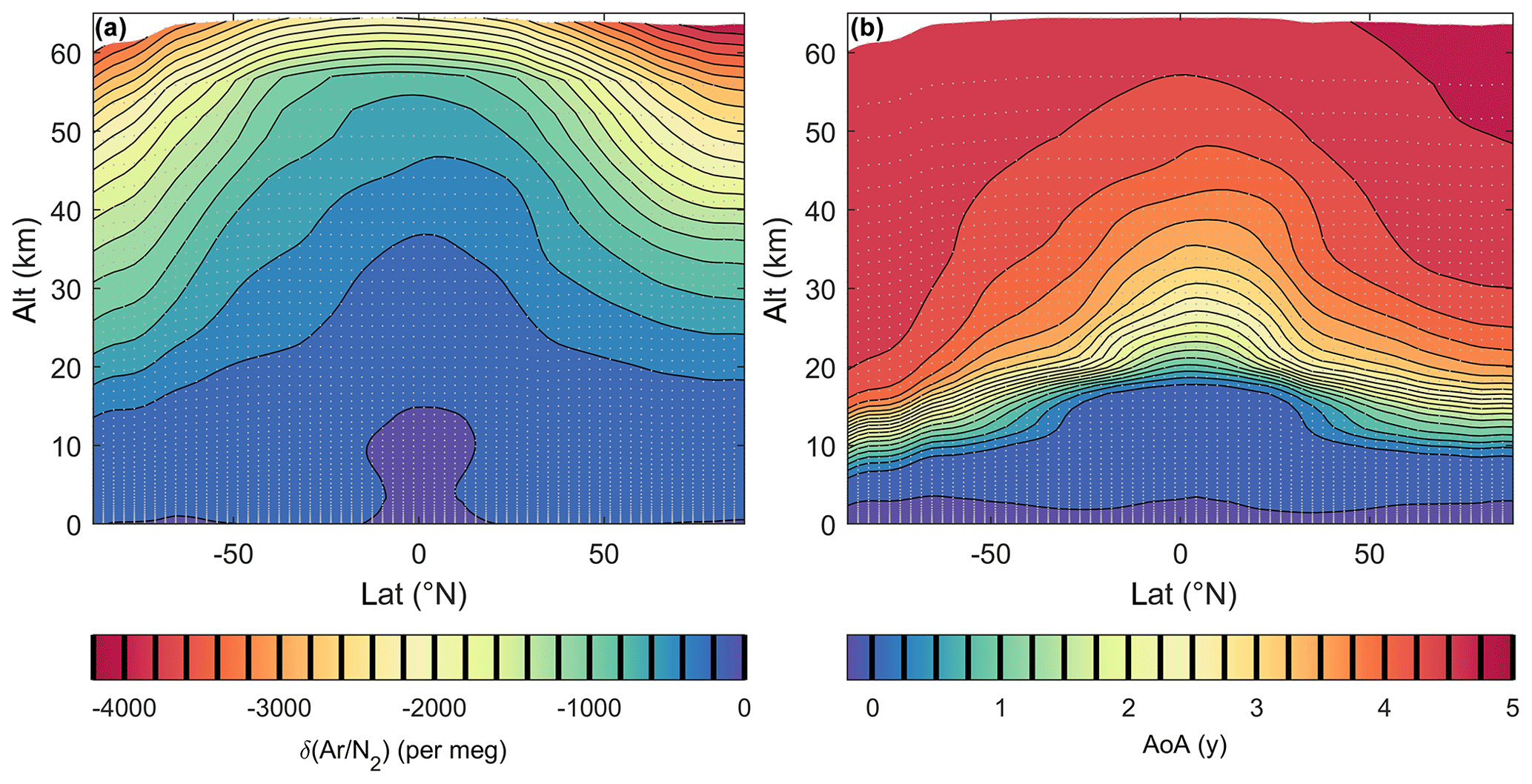
Figure 6 Annual and zonal means of δ(Ar∕N₂) (a) and age of air (AoA) (b) simulated by TOMCAT. Values of the contour lines are shown as black vertical lines on the color bar. Grey dots indicate the center of a grid box in TOMCAT. A video of this figure highlighting the natural variability in monthly-mean values is available in the Supplement.

The AoA tracer in TOMCAT shows a similar pattern to δ(Ar∕N₂), with younger ages at low altitude and in the tropics and the oldest ages in the mesosphere. Vertical gradients in mean AoA are largest at high latitudes close to the tropopause. At high latitudes above 20 km and at low latitudes above 50 km, vertical gradients of AoA mostly disappear and AoA becomes nearly uniform.

4 Discussion

4.1 Difference between TOMCAT and the NIES TM

We hypothesize that an adequate representation of the mesosphere in models is critical in determining the curvature of the AoA–GS relationship. The residence time of air above ∼40 km is rather short in TOMCAT, and AoA is nearly constant with altitude in this region. GS in contrast continues to increase with altitude because of the diffusivity dependence on pressure allowing gases to separate more effectively. The much lower top of the NIES TM (∼35 km vs. 60–65 km) reduces its ability to capture this effect, which impacts the AoA–GS relationship because the mesospheric signal is exported into the stratosphere, in particular in polar regions where mesospheric air descends. TOMCAT furthermore produces a less negative slope of the AoA–GS relationship for young air (mean AoA <3 years) and greater similarity in the AoA–GS relationship between latitude bands than the NIES TM as shown in Fig. 5. This could in part be a consequence of using a different meteorological reanalysis product for forcing the two models (Chabrillat et al., 2018) or could indicate differences between the models in vertical and horizontal mixing intensity.

4.2 Estimating mean AoA from observed δ(Ar∕N₂)

Different tracers of AoA all have unique strengths and weaknesses. Estimating AoA in the lowermost stratosphere from CO₂ for example is limited by complexities involving seasonality and the possibility of multiple entry points of air into the stratosphere due to isentropic mixing with the midlatitude troposphere (Hall and Plumb, 1994; Andrews et al., 2001; Waugh and Hall, 2002). SF₆-derived AoA in contrast is biased high at mid and high latitudes due to the influence of mesospheric air which has been photochemically depleted in SF₆ (Kovács et al., 2017; Linz et al., 2017). N₂O as an AoA tracer relies on the photolytic destruction of N₂O in the stratosphere, which may depend strongly on location and had only been empirically calibrated for young ages at mid latitudes so far (Andrews et al., 2001; Linz et al., 2017).

Thanks to the robust relationship between mean AoA and δ(Ar∕N₂) and the small seasonal cycle amplitude of $\mathit{\delta }(\mathrm{Ar}/{\mathrm{N}}_{\mathrm{2}})<\mathrm{5}$ per meg in the upper troposphere (Fig. S1), mean AoA could also be estimated from δ(Ar∕N₂). Using the current analytical δ(Ar∕N₂) uncertainty of 12.2 per meg (2σ) and the AoA–δ(Ar∕N₂) relationship seen in TOMCAT (including variability from seasonal and latitudinal differences), we estimate that mean AoA could be calculated to within about ±0.4 years (2σ, Fig. S5). This is still considerably worse than the ±0.1-year confidence interval in mean AoA estimated from N₂O. However, the uncertainty can be improved with future improvements in sampling, and the accuracy and precision of the measurements.

The heavy noble gases krypton and xenon will be roughly 3.6× and 5.8× more strongly fractionated in the stratosphere than Ar but are also more challenging to measure due to their ∼ 8000× and 100 000× lower abundance in the atmosphere. Nevertheless, future analysis of these gases in stratospheric air samples might further improve our ability to estimate AoA from the gravitational fractionation of gases and help diagnose artifactual fractionation, because heavier noble gases are more strongly fractionated under the influence of gravity and less sensitive to thermal fractionation (Seltzer et al., 2019).

4.3 Future directions

An open question in climate applications of noble gases is whether there could be a stratospheric influence on tropospheric δ(Ar∕N₂). Tropospheric observations of δ(Ar∕N₂) and other noble gas-elemental ratios have been used to infer ocean heat content changes by capitalizing on the temperature dependency of gas solubility in the oceans (Keeling et al., 2004; Headly and Severinghaus, 2007; Ritz et al., 2011; Bereiter et al., 2018). However, long-term trends (Butchart, 2014) and natural variability in stratospheric circulation and stratosphere–troposphere exchange (STE) such as the Quasi-Biennial Oscillation (QBO) (Baldwin et al., 2001) could advect a stratospheric GS signal into the troposphere and alias onto surface observations of these gases. To this end, we calculate the volumetric Ar deficit in the atmosphere in moles using TOMCAT (Fig. 7) relative to a hypothetical, unfractionated atmosphere with a homogenous mixing ratio ($C_{{\mathrm{o}}_{\mathrm{Ar}}}$) at all elevations. Ar deficit is

$$\begin{array}{}\text{(6)}& {\mathrm{Ar}}_{\mathrm{deficit}}=\left(C_{\mathrm{Ar}}-C_{{\mathrm{o}}_{\mathrm{Ar}}}\right)\times N_{\mathrm{air}},\end{array}$$

where C_Ar is the simulated Ar mixing ratio and N_air is the number density of air.

Figure 7 Color map of annual mean and zonally integrated Ar deficit in TOMCAT. Overlain black contour lines show δ(Ar∕N₂) (per meg). The red solid line highlights the mean position of the 200 hPa isobar.

The Ar deficit is concentrated in the lower stratosphere at around 20 km and at mid to high latitudes. Although the GS signal is considerably stronger in the mesosphere, the potential for perturbing the troposphere is low given the low molar density of air in the mesosphere. The region with the greatest potential to influence the troposphere therefore lies in the lower stratosphere. The total Ar deficit of the atmosphere above 200 hPa is approximately $-\mathrm{2.9}\times {\mathrm{10}}^{\mathrm{13}}$ mol and the atmosphere below 200 hPa contains roughly 1.3×10¹⁸ mol of Ar. Perturbing STE and/or the stratospheric circulation by 10 %, consistent with interannual to decadal variability of STE in models (Salby and Callaghan, 2006; Flury et al., 2013; Ray et al., 2014; Montzka et al., 2018), thus should lead to a detectable signal of roughly 2.2 per meg ($-\mathrm{2.9}\times {\mathrm{10}}^{\mathrm{13}}/\mathrm{1.3}\times {\mathrm{10}}^{\mathrm{18}}\times \mathrm{10}\mathit{\%}\times {\mathrm{10}}^{\mathrm{6}}$) in tropospheric δ(Ar∕N₂). Corresponding advection of stratospheric GS signals in N₂ amplifies the pure Ar signal by roughly 10 %. A careful investigation of such a signal in the δ(Ar∕N₂) surface network data (Keeling et al., 2004) is needed because secular trends of δ(Ar∕N₂) caused by degassing of Ar and N₂ from a warming ocean are also expected to be on the order of 2–3 per meg per decade. Previous studies have also used ratios involving heavier noble gases (Xe∕N₂, Kr∕N₂) to reconstruct mean ocean temperature changes over glacial–interglacial timescales (Headly and Severinghaus, 2007; Bereiter et al., 2018; Baggenstos et al., 2019). Simultaneous changes in stratospheric circulation and STE affect heavier noble gases more strongly than Ar∕N₂ and will need to be accounted for in such applications of noble gas thermometry.

5 Conclusions

With improvements in data treatment, measurement quality, and modeling constraints, we have shown that gravitational fractionation of Ar relative to N₂ in the stratosphere and mesosphere is a potentially powerful constraint on circulation. High-precision observations of δ(Ar∕N₂) in air samples of the lowermost stratosphere from nine airborne campaigns are well captured by the TOMCAT/SLIMCAT 3-D chemical transport model, which has been updated to account for the influence of gravity on air composition through molecular diffusion. In the observations and the model, δ(Ar∕N₂) is directly related to stratospheric mean age of air (AoA) derived here using a new calibration of N₂O. Our observations for mean AoA <3 years produce a slope of roughly 35–45 per meg of δ(Ar∕N₂) per year of AoA. TOMCAT/SLIMCAT shows better agreement with the new observations than the NIES transport model (Belikov et al., 2019), and we speculate that the model disagreement could be explained by (i) the factor of 2 lower top of the NIES transport model, (ii) the use of different reanalysis products, and/or (iii) differences in vertical and horizontal mixing. In this context, further work is also needed to study the influence of unresolved turbulence on AoA and δ(Ar∕N₂) in chemical transport models.

As the importance of stratospheric circulation for ozone recovery, climate projections, and evaluation of tropospheric trends in halocarbons is increasingly recognized, a need for new observations from the still undersampled stratosphere is becoming evident. Combining δ(Ar∕N₂) with other tracers of circulation could lead to new insights into atmospheric mixing and transport. δ(Ar∕N₂) has potential advantages over existing approaches based on transient tracers such as CO₂ or N₂O since δ(Ar∕N₂) is only influenced by the physics of transport and mostly unaffected by seasonality in the tropical upper troposphere. Furthermore, because of its large gradients at high altitudes, δ(Ar∕N₂) observations from the upper stratosphere and mesosphere could improve our understanding of circulation on seasonal and interannual timescales in a region where AoA becomes near uniform, and some photochemical age tracers such as N₂O are almost fully depleted and thus lose sensitivity to circulation changes.

Appendix A: Description of the Markov chain Monte Carlo algorithm

The following list outlines key steps in our MCMC algorithm to calculate AoA from CO₂ for each N₂O bin.

1. Start a new Markov chain and allow for uncertainty in TRTS by adding white noise with an amplitude given by the scatter of upper tropospheric observations around the mean TRTS in Fig. 2.

2. With a 50 % chance, peak weighting factor A is set to zero and a unimodal spectrum is tested (k=1). Alternatively, A is allowed to vary between 0 and 1 for a bimodal distribution (k=2).

3. The other age spectrum parameters are selected from N₂O bin-dependent prior distributions: Γ₁ is sampled from a uniform prior distribution with a mean AoA predicted by the N₂O–AoA relationship of Andrews et al. (2001) and with generous width (>1.5 years). Γ₂ is sampled from a uniform prior distribution with values between 1 and 6 years representing older stratospheric air. The shape parameters are defined as ${\mathit{\lambda }}_i\equiv \frac{{\mathrm{\Gamma }}_i^{\mathrm{2}}}{\mathrm{2}{\mathit{\gamma }}_i}$, and γ_i is chosen randomly for each peak with values between 0.1 and 1, as observed in previous studies (Hall and Plumb, 1994; Andrews et al., 2001; Waugh and Hall, 2002).

4. Convolve the age spectrum calculated from the parameters ($\mathit{m}\equiv \left[{\mathrm{\Gamma }}_{\mathrm{1}},{\mathrm{\Gamma }}_{\mathrm{2}},{\mathit{\lambda }}_{\mathrm{1}},{\mathit{\lambda }}_{\mathrm{2}},A\right])$ with the perturbed TRTS to obtain a possible time series of CO₂ in the N₂O bin and calculate the misfit (e) between the CO₂ time series and observations.

5. Calculate the likelihood function P(d|k,m) for the set of parameters m and k, given a total of n observations (d):

   $$\begin{array}{}\text{(A1)}& \begin{array}{rl}P& \left(\mathit{d}\mathrm{|}k,\mathit{m}\right)=\\ & {\displaystyle \frac{\mathrm{1}}{{\left[{\left(\mathrm{2}\mathit{\pi }\right)}^n\det \left({\widehat{\mathbf{C}}}_{\mathbf{e}}\right)\right]}^{\mathrm{0.5}}}}\exp \left(-{\displaystyle \frac{\mathrm{1}}{\mathrm{2}}}{\mathbf{e}}^T{\widehat{\mathbf{C}}}_{\mathbf{e}}^{-\mathrm{1}}\mathit{e}\right).\end{array}\end{array}$$

   where ${\widehat{\mathbf{C}}}_{\mathbf{e}}$ is the covariance matrix. We assume that all n observations are independent. Thus, ${\widehat{\mathbf{C}}}_{\mathbf{e}}$ has only diagonal entries of ${\mathit{\sigma }}_{{\mathrm{CO}}_{\mathrm{2}}}^{\mathrm{2}}$ and $\det \left({\widehat{\mathbf{C}}}_{\mathbf{e}}\right)$ simplifies to $({\mathit{\sigma }}_{{\mathrm{CO}}_{\mathrm{2}}}^{\mathrm{2}}{)}^n$. The value of ${\mathit{\sigma }}_{{\mathrm{CO}}_{\mathrm{2}}}^{\mathrm{2}}$ is different for each bin and determined iteratively as the approximate root mean square error of the observations around the final time series for each bin obtained at the end of the MCMC algorithm. Typical values of ${\mathit{\sigma }}_{{\mathrm{CO}}_{\mathrm{2}}}^{\mathrm{2}}$ are between 0.18 and 1.28 ppm and generally decrease with increasing AoA of a N₂O bin.

6. If this is the first pass of the chain, define k_saved and m_saved to equal k and m. Otherwise, calculate the selection criterion $\mathit{\alpha }\equiv min\left(\mathrm{1},\frac{P\left(\mathit{d}\mathrm{|}k,\mathit{m}\right)}{P\left(\mathit{d}\mathrm{|}{k}_{\mathrm{saved}},{\mathit{m}}_{\mathrm{saved}}\right)}\right)$ and accept k and m as new saved values (k_savedm_saved) with probability α. Sampling from the same prior distributions on each pass of the chain simplifies our expression of α compared to that presented by Malinverno (2002), making it only dependent on the likelihood ratio.

7. Repeat steps 2–6 1000 times, sampling parameter values from the same prior distributions, and store the final values of k_saved and m_saved obtained after the 1000th iteration (i.e., a plausible solution produced past the burn-in period) for later use.

8. To sample the full posterior pdf (i.e., the full uncertainty about the age spectrum parameters), initialize 2000 different Markov chains by repeating steps 1–7. Each stored value of m characterizes one age spectrum that is likely not far from the best solution, given the data d, yielding an ensemble of 2000 age spectra from which statistics can be computed. Note that each Markov chain is fully independent, so the algorithm can be easily parallelized to minimize computational costs.

Appendix B: Derivation of Eq. (4) from the Maxwell–Stefan equations

We start by approximating air as a ternary mixture of N₂, O₂, and Ar and later generalize to consider additional trace species. According to the Maxwell–Stefan equations (Taylor and Krishna, 1993), diffusion in this ternary mixture is governed by

$$\begin{array}{}\text{(B1)}& {\displaystyle }{\mathit{d}}_{{\mathrm{N}}_{\mathrm{2}}}={\displaystyle \frac{C_{{\mathrm{N}}_{\mathrm{2}}}{\mathit{f}}_{\mathrm{Ar}}-C_{\mathrm{Ar}}{\mathit{f}}_{{\mathrm{N}}_{\mathrm{2}}}}{N\times D_{{\mathrm{N}}_{\mathrm{2}}:\mathrm{Ar}}}}+{\displaystyle \frac{C_{{\mathrm{N}}_{\mathrm{2}}}{\mathit{f}}_{{\mathrm{O}}_{\mathrm{2}}}-C_{{\mathrm{O}}_{\mathrm{2}}}{\mathit{f}}_{{\mathrm{N}}_{\mathrm{2}}}}{N\times D_{{\mathrm{N}}_{\mathrm{2}}:{\mathrm{O}}_{\mathrm{2}}}}},\text{(B2)}& {\displaystyle }{\mathit{d}}_{\mathrm{Ar}}={\displaystyle \frac{C_{\mathrm{Ar}}{\mathit{f}}_{{\mathrm{N}}_{\mathrm{2}}}-C_{{\mathrm{N}}_{\mathrm{2}}}{\mathit{f}}_{\mathrm{Ar}}}{N\times D_{\mathrm{Ar}:{\mathrm{N}}_{\mathrm{2}}}}}+{\displaystyle \frac{C_{\mathrm{Ar}}{\mathit{f}}_{{\mathrm{O}}_{\mathrm{2}}}-C_{{\mathrm{O}}_{\mathrm{2}}}{\mathit{f}}_{\mathrm{Ar}}}{N\times D_{\mathrm{Ar}:{\mathrm{O}}_{\mathrm{2}}}}},\text{(B3)}& {\displaystyle }{\mathit{f}}_{{\mathrm{O}}_{\mathrm{2}}}=-{\mathit{f}}_{{\mathrm{N}}_{\mathrm{2}}}-{\mathit{f}}_{\mathrm{Ar}},\text{(B4)}& {\displaystyle }{C}_{{\mathrm{N}}_{\mathrm{2}}}+C_{{\mathrm{O}}_{\mathrm{2}}}+C_{\mathrm{Ar}}=\mathrm{1},\end{array}$$

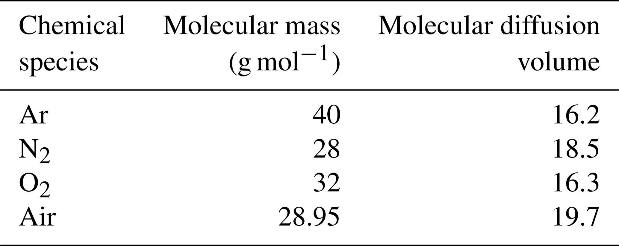
where $C_i\equiv n_i/N$ is the mole fraction, n_i is molar or number density (mol m⁻³), N is the total number density (mol m⁻³), f_i is the molecular diffusion flux (mol m² s⁻¹) relative to the molar average velocity of the mixture, d_i is the thermodynamic driving force for molecular diffusion (m⁻¹), and D_i:j is the binary diffusion coefficient of the (i:j) pair. An equation for O₂ that is analogous to Eq. (B1) is not needed because changes in O₂ are governed by the conservation Eqs. (B3) and (B4). Binary diffusivity coefficients (cm² s⁻¹) can be calculated using the method of Fuller et al. as reported in Reid et al. (1987):

$$\begin{array}{}\text{(B5)}& D_{ij}=\mathrm{0.001}{\displaystyle \frac{T^{\mathrm{1.75}}{\left(\frac{\mathrm{1}}{M_i}+\frac{\mathrm{1}}{M_j}\right)}^{\mathrm{0.5}}}{P{\left[{\mathit{\nu }}_i^{\mathrm{1}/\mathrm{3}}+{\mathit{\nu }}_j^{\mathrm{1}/\mathrm{3}}\right]}^{\mathrm{2}}}},\end{array}$$

where P is pressure (atm), ν_i is the molecular diffusion volume of a trace gas or air (Table B1), and M_i is the molecular mass (g mol⁻¹) of a gas.

Table B1 Molecular diffusion volumes (Reid et al., 1987) and masses used in this study.

For an ideal gas, d_i is given by

$$\begin{array}{}\text{(B6)}& \begin{array}{rl}{d}_i& \equiv \mathrm{\nabla }{C}_i+\left(C_i-{\mathit{\omega }}_i\right){\displaystyle \frac{\mathrm{\nabla }P}{P}}-{\displaystyle \frac{{\mathit{\rho }}_i}{P}}\left({\displaystyle \frac{F_i}{M_i}}-\sum _{j=\mathrm{1}}^n{\mathit{\omega }}_i{\displaystyle \frac{F_j}{M_j}}\right)\\ & +{\displaystyle \frac{k_i^T}{T}}\mathrm{\nabla }T,\end{array}\end{array}$$

where ${\mathit{\omega }}_i\equiv \frac{{\mathit{\rho }}_i}{\mathit{\rho }}=\frac{M_i{C}_i}{M_{\mathrm{air}}}$ is the mass fraction of gas i, ρ_i is density of i (kg m⁻³), P is pressure (Pa), T is temperature (K), $k_i^T$ is the thermal-diffusion ratio of i, M_i is the molecular mass of i (kg mol⁻¹), and F_i the external body force per mole (N mol⁻¹) for i (Chapman et al., 1990; Taylor and Krishna, 1993).

In the atmosphere, (vertical) pressure gradients are caused by gravity and well approximated by hydrostatic balance

$$\begin{array}{}\text{(B7)}& \mathrm{\nabla }P\approx {\displaystyle \frac{\partial P}{\partial z}}\approx -\mathit{\rho }g=-{\displaystyle \frac{P{M}_{\mathrm{air}}}{RT}}g.\end{array}$$

The gravitational force per mole F_i is

$$\begin{array}{}\text{(B8)}& F_i=-{\displaystyle \frac{{\mathit{\rho }}_i}{n_i}}g.\end{array}$$

Substituting Eqs. (B7) and (B8) into Eq. (B6) yields

$$\begin{array}{}\text{(B9)}& \begin{array}{rl}{d}_i& \approx \mathrm{\nabla }{C}_i-\left(\mathrm{1}-{\displaystyle \frac{M_i}{M_{\mathrm{air}}}}\right)C_i{\displaystyle \frac{\mathrm{1}}{P}}{\displaystyle \frac{P{M}_{\mathrm{air}}g}{RT}}\\ & +{\displaystyle \frac{{\mathit{\rho }}_i}{P}}\left({\displaystyle \frac{\frac{{\mathit{\rho }}_i}{n_i}g}{M_i}}-\sum _{j=\mathrm{1}}^n{\mathit{\omega }}_j{\displaystyle \frac{\frac{{\mathit{\rho }}_j}{n_j}g}{M_j}}\right)+{\displaystyle \frac{k_i^T}{T}}\mathrm{\nabla }T\\ & =\mathrm{\nabla }{C}_i+\left(M_i-M_{\mathrm{air}}\right){\displaystyle \frac{g}{RT}}{C}_i+{\displaystyle \frac{{\mathit{\rho }}_i}{P}}\left(g-\sum _{j=\mathrm{1}}^n{\mathit{\omega }}_{i}g\right)\\ & +{\displaystyle \frac{k_i^T}{T}}\mathrm{\nabla }T\\ & =\mathrm{\nabla }{C}_i+\left({\displaystyle \frac{\mathrm{1}}{H_i}}-{\displaystyle \frac{\mathrm{1}}{H_{\mathrm{air}}}}\right)C_i+{\displaystyle \frac{k_i^T}{T}}\mathrm{\nabla }T,\end{array}\end{array}$$

where we use the definition of the scale height $H_i\equiv \frac{RT}{g{M}_i}$. The two terms involving the body force cancel because all species experience the same gravitational force per unit mass. The tendency for gravimetric separation instead arises from the pressure gradient term proportional to $\left(\frac{\mathrm{1}}{H_i}-\frac{\mathrm{1}}{H_{\mathrm{air}}}\right)$.

Equations (B1) and (B2) can be inverted to solve for $f_{{\mathrm{N}}_{\mathrm{2}}}$ and f_Ar (Taylor and Krishna, 1993):

$$\begin{array}{}\text{(B10)}& {\displaystyle }{f}_{{\mathrm{N}}_{\mathrm{2}}}=-N{D}_{{\mathrm{N}}_{\mathrm{2}}}^{\mathrm{air}}{d}_{{\mathrm{N}}_{\mathrm{2}}}-N{D}_{{\mathrm{N}}_{\mathrm{2}}\times (\mathrm{Ar},{\mathrm{O}}_{\mathrm{2}})}^{\mathrm{air}}{d}_{\mathrm{Ar}},\text{(B11)}& {\displaystyle }{f}_{\mathrm{Ar}}=-N{D}_{\mathrm{Ar}\times ({\mathrm{N}}_{\mathrm{2}},{\mathrm{O}}_{\mathrm{2}})}^{\mathrm{air}}{d}_{{\mathrm{N}}_{\mathrm{2}}}-N{D}_{\mathrm{Ar}}^{\mathrm{air}}{d}_{\mathrm{Ar}},\end{array}$$

where

$$\begin{array}{}\text{(B12)}& {\displaystyle }{D}_{{\mathrm{N}}_{\mathrm{2}}}^{\mathrm{air}}={\displaystyle \frac{D_{{\mathrm{N}}_{\mathrm{2}}:\mathrm{O}\mathrm{2}}\left(C_{{\mathrm{N}}_{\mathrm{2}}}{D}_{\mathrm{Ar}:{\mathrm{O}}_{\mathrm{2}}}+\left(\mathrm{1}-C_{{\mathrm{N}}_{\mathrm{2}}}\right)D_{{\mathrm{N}}_{\mathrm{2}}:\mathrm{Ar}}\right)}{S}},\text{(B13)}& {\displaystyle }{D}_{{\mathrm{N}}_{\mathrm{2}}\times (\mathrm{Ar},{\mathrm{O}}_{\mathrm{2}})}^{\mathrm{air}}={\displaystyle \frac{C_{{\mathrm{N}}_{\mathrm{2}}}{D}_{\mathrm{Ar}:{\mathrm{O}}_{\mathrm{2}}}\left(D_{{\mathrm{N}}_{\mathrm{2}}:\mathrm{O}\mathrm{2}}-D_{{\mathrm{N}}_{\mathrm{2}}:\mathrm{Ar}}\right)}{S}},\text{(B14)}& {\displaystyle }{D}_{\mathrm{Ar}}^{\mathrm{air}}={\displaystyle \frac{D_{\mathrm{Ar}:{\mathrm{O}}_{\mathrm{2}}}\left(C_{\mathrm{Ar}}{D}_{{\mathrm{N}}_{\mathrm{2}}:{\mathrm{O}}_{\mathrm{2}}}+\left(\mathrm{1}-C_{\mathrm{Ar}}\right)D_{{\mathrm{N}}_{\mathrm{2}}:\mathrm{Ar}}\right)}{S}},\text{(B15)}& {\displaystyle }{D}_{\mathrm{Ar}\times ({\mathrm{N}}_{\mathrm{2}},{\mathrm{O}}_{\mathrm{2}})}^{\mathrm{air}}={\displaystyle \frac{C_{\mathrm{Ar}}{D}_{{\mathrm{N}}_{\mathrm{2}}:{\mathrm{O}}_{\mathrm{2}}}\left(D_{\mathrm{Ar}:{\mathrm{O}}_{\mathrm{2}}}-D_{{\mathrm{N}}_{\mathrm{2}}:\mathrm{Ar}}\right)}{S}},\text{(B16)}& {\displaystyle }S=C_{{\mathrm{N}}_{\mathrm{2}}}{D}_{\mathrm{Ar}:{\mathrm{O}}_{\mathrm{2}}}+C_{\mathrm{Ar}}{D}_{{\mathrm{N}}_{\mathrm{2}}:{\mathrm{O}}_{\mathrm{2}}}+C_{{\mathrm{O}}_{\mathrm{2}}}{D}_{{\mathrm{N}}_{\mathrm{2}}:\mathrm{Ar}}.\end{array}$$

Here $D_{{\mathrm{N}}_{\mathrm{2}}}^{\mathrm{air}}$ and $D_{\mathrm{Ar}}^{\mathrm{air}}$ are the effective diffusivities of N₂ and Ar in air, while $D_{{\mathrm{N}}_{\mathrm{2}}\times (\mathrm{Ar},{\mathrm{O}}_{\mathrm{2}})}^{\mathrm{air}}$ and $D_{\mathrm{Ar}\times ({\mathrm{N}}_{\mathrm{2}},{\mathrm{O}}_{\mathrm{2}})}^{\mathrm{air}}$ reflect ternary cross-interactions, such as the tendency of N₂ to be impacted by any process that drives a diffusive flux of Ar.

Table B2 Characteristic values of variables in Eqs. (B19) and (B20).

^a $\mathrm{1.8}\times {\mathrm{10}}^{-\mathrm{2}}$ observed at 293 K (Waldmann, 1947). ^b Assuming $C_{\mathrm{Ar}}\approx \frac{N_{\mathrm{Ar}}}{N_{{\mathrm{N}}_{\mathrm{2}}}}$. ^c Estimated from TOMCAT results.

In air, Ar is a minor gas ($C_{\mathrm{Ar}}\ll C_{{\mathrm{N}}_{\mathrm{2}}}\sim C_{{\mathrm{O}}_{\mathrm{2}}}$), and therefore interactions of N₂ with Ar can be neglected in the N₂ flux and the diffusive fluxes of N₂ and O₂ must balance approximately, as in the case of a binary mixture of the two gases:

$$\begin{array}{}\text{(B17)}& {\displaystyle }{f}_{{\mathrm{N}}_{\mathrm{2}}}\approx -N{D}_{{\mathrm{N}}_{\mathrm{2}}}^{\mathrm{air}}{d}_{{\mathrm{N}}_{\mathrm{2}}},\text{(B18)}& {\displaystyle }{f}_{{\mathrm{O}}_{\mathrm{2}}}\approx -f_{{\mathrm{N}}_{\mathrm{2}}}.\end{array}$$

Combining Eqs. (B10) and (B17) with Eq. (B9) yields

$$\begin{array}{}\text{(B19)}& {\displaystyle }\begin{array}{rl}{f}_{{\mathrm{N}}_{\mathrm{2}}}& \approx -N{D}_{{\mathrm{N}}_{\mathrm{2}}}^{\mathrm{air}}[\mathrm{\nabla }{C}_{{\mathrm{N}}_{\mathrm{2}}}+\left({\displaystyle \frac{\mathrm{1}}{H_{{\mathrm{N}}_{\mathrm{2}}}}}-{\displaystyle \frac{\mathrm{1}}{H_{\mathrm{air}}}}\right)C_{{\mathrm{N}}_{\mathrm{2}}}\\ & +{\mathit{\alpha }}_{{\mathrm{N}}_{\mathrm{2}}:{\mathrm{O}}_{\mathrm{2}}}^T{\displaystyle \frac{C_{{\mathrm{N}}_{\mathrm{2}}}\left(\mathrm{1}-C_{{\mathrm{N}}_{\mathrm{2}}}\right)}{T}}\mathrm{\nabla }T],\end{array}\text{(B20)}& {\displaystyle }\begin{array}{rl}{f}_{\mathrm{Ar}}& \approx -N{D}_{\mathrm{Ar}\times ({\mathrm{N}}_{\mathrm{2}},{\mathrm{O}}_{\mathrm{2}})}^{\mathrm{air}}[\mathrm{\nabla }{C}_{{\mathrm{N}}_{\mathrm{2}}}+\left({\displaystyle \frac{\mathrm{1}}{H_{{\mathrm{N}}_{\mathrm{2}}}}}-{\displaystyle \frac{\mathrm{1}}{H_{\mathrm{air}}}}\right)C_{{\mathrm{N}}_{\mathrm{2}}}\\ & +{\mathit{\alpha }}_{{\mathrm{N}}_{\mathrm{2}}:{\mathrm{O}}_{\mathrm{2}}}^T{\displaystyle \frac{C_{{\mathrm{N}}_{\mathrm{2}}}\left(\mathrm{1}-C_{{\mathrm{N}}_{\mathrm{2}}}\right)}{T}}\mathrm{\nabla }T]\\ & -N{D}_{\mathrm{Ar}}^{\mathrm{air}}[\mathrm{\nabla }{C}_{\mathrm{Ar}}+\left({\displaystyle \frac{\mathrm{1}}{H_{\mathrm{Ar}}}}-{\displaystyle \frac{\mathrm{1}}{H_{\mathrm{air}}}}\right)C_{\mathrm{Ar}}\\ & +{\mathit{\alpha }}_{\mathrm{Ar}:\mathrm{air}}^T{\displaystyle \frac{C_{\mathrm{Ar}}}{T}}\mathrm{\nabla }T],\end{array}\end{array}$$

where we have replaced the thermal diffusion ratio $k_i^T$ with the better empirically constrained thermal diffusion factor ${\mathit{\alpha }}_i^T\equiv \frac{k_i^T}{C_i{C}_j}$ defined as such only in binary mixtures. Therefore, $k_{{\mathrm{N}}_{\mathrm{2}}}^T\approx {\mathit{\alpha }}_{{\mathrm{N}}_{\mathrm{2}}:\mathrm{O}\mathrm{2}}^T{C}_{{\mathrm{N}}_{\mathrm{2}}}{C}_{{\mathrm{O}}_{\mathrm{2}}}$ and $k_{\mathrm{Ar}}^T\approx {\mathit{\alpha }}_{\mathrm{Ar}:\mathrm{air}}^T{C}_{\mathrm{Ar}}$. Table B2 presents rough estimates of the magnitudes of the terms in Eqs. (B19) and (B20) in the stratosphere, showing that the thermal diffusion and cross-diffusion terms involving $D_{\mathrm{Ar}\times ({\mathrm{N}}_{\mathrm{2}},{\mathrm{O}}_{\mathrm{2}})}^{\mathrm{air}}$ are at least 2 orders of magnitude smaller than the remaining terms. Neglecting these smaller terms yields the governing Eq. (4) used in our model simulation:

$$\begin{array}{}\text{(B21)}& \begin{array}{rl}{\mathit{f}}_{\mathit{i}}& \approx -N{D}_i\left[\left({\displaystyle \frac{\mathrm{1}}{H_i}}-{\displaystyle \frac{\mathrm{1}}{H_{\mathrm{air}}}}\right)C_i\right]\\ & =-N{D}_i\mathrm{\Delta }{M}_i{\displaystyle \frac{g}{RT}}{C}_i,\end{array}\end{array}$$

where we introduced $\mathrm{\Delta }{M}_i\equiv M_i-M_{\mathrm{air}}$, the molecular mass difference to air (kg mol⁻¹), as a shorthand. Equation (B21) is equally valid for trace gases such as Ar and major gases N₂ and O₂ when the appropriate diffusivities given by Eqs. (B12) and (B14) are used. In our case $D_{{\mathrm{N}}_{\mathrm{2}}}\equiv D_{{\mathrm{N}}_{\mathrm{2}}}^{\mathrm{air}}=D_{{\mathrm{O}}_{\mathrm{2}}}^{\mathrm{air}}\approx D_{{\mathrm{N}}_{\mathrm{2}}:{\mathrm{O}}_{\mathrm{2}}}$ for N₂ and $D_{\mathrm{Ar}}\equiv D_{\mathrm{Ar}}^{\mathrm{air}}\approx \frac{D_{\mathrm{Ar}:{\mathrm{O}}_{\mathrm{2}}}{D}_{{\mathrm{N}}_{\mathrm{2}}:\mathrm{Ar}}}{C_{{\mathrm{N}}_{\mathrm{2}}}{D}_{\mathrm{Ar}:{\mathrm{O}}_{\mathrm{2}}}+C_{{\mathrm{O}}_{\mathrm{2}}}{D}_{{\mathrm{N}}_{\mathrm{2}}:\mathrm{Ar}}}$ for Ar.

Appendix C: Calculating δ(Ar∕N₂) from δ(GST)

The conservation equation of gas i with mixing ratio C_i accounting for advection (first term RHS), eddy mixing (second term RHS), and molecular diffusion (third term RHS, using the simplified Eq. B21) is given by

$$\begin{array}{}\text{(C1)}& \begin{array}{rl}{\displaystyle \frac{\partial }{\partial t}}& \left(C_i\right)=-\mathit{u}\cdot \mathbf{\nabla }\left[C_i\right]+\mathbf{\nabla }\cdot \left[{\mathbf{D}}_e\mathbf{\nabla }{C}_i\right]\\ & +{\displaystyle \frac{\partial }{\partial z}}\left[D_i\mathrm{\Delta }{M}_i{\displaystyle \frac{g}{RT}}{C}_i\right],\end{array}\end{array}$$

where u is the velocity vector (m s⁻¹), D_e is the eddy diffusivity tensor (m² s⁻¹), D_i is the molecular diffusivity of species i in air (i.e., $D_i^{\mathrm{air}}$ m² s⁻¹), g is the gravitational acceleration, R is the fundamental gas constant (J K⁻¹ mol⁻¹), and T is temperature (K). “∇⋅” represents the divergence operator. u, D_e, D_i, N, and T depend on x, y, z, and t and the largest gradients for these variables generally occur in the vertical direction.

Dividing Eq. (C1) by a reference value C_i,0, separating C_i into a constant and a perturbation component (i.e., $\frac{C_i}{C_{i,\mathrm{0}}}=\mathrm{1}+\frac{C_i^{\prime }}{C_{i,\mathrm{0}}}=\mathrm{1}+{\mathit{\delta }}_i$), and using the chain rule yields

$$\begin{array}{}\text{(C2)}& \begin{array}{rl}{\displaystyle \frac{\partial }{\partial t}}& \left({\mathit{\delta }}_i\right)=-\mathit{u}\cdot \mathbf{\nabla }\left[{\mathit{\delta }}_i\right]+\mathbf{\nabla }\cdot \left[{\mathbf{D}}_e\mathbf{\nabla }{\mathit{\delta }}_i\right]\\ & +D_i\mathrm{\Delta }{M}_i{\displaystyle \frac{g}{RT}}{\displaystyle \frac{\partial }{\partial z}}\left[{\mathit{\delta }}_i\right]+\left(\mathrm{1}+{\mathit{\delta }}_i\right){\displaystyle \frac{\partial }{\partial z}}\left[D_i\mathrm{\Delta }{M}_i{\displaystyle \frac{g}{RT}}\right].\end{array}\end{array}$$

To simplify Eq. (C2), we assume that the perturbations in the mixing ratio are small (i.e., δ_i≪1), which is true at the 1 % level for δ(Ar∕N₂) even in the mesosphere. Furthermore, we assume that $U+\frac{D_e}{L}\gg \frac{D_i}{\mathrm{\Delta }{H}_i}$ (U is a characteristic velocity scale, D_e is a characteristic eddy diffusivity, and L is a characteristic length scale; $\mathrm{\Delta }{H}_i=\frac{RT}{\mathrm{\Delta }{M}_{i}g}$) or, equivalently stated in terms of the Peclet number, $\mathit{\text{Pe}}\sim \frac{U\mathrm{\Delta }{H}_i+D_e\frac{\mathrm{\Delta }{H}_i}{L}}{D_i}\gg \mathrm{1}$. We estimate typical values of the vertical Peclet number in the stratosphere to be between 1000 and 10 000 based on the height (∼20 km) and turnover time (∼5 years) of the stratosphere and the range of molecular diffusivities given in Table B1. In the mesosphere, AoA is near uniform, and we conservatively assume a turnover time of 0.5 years and a height of 20 km. This implies a Peclet number of ∼500 for the mesosphere. Under these conditions, the third term on the RHS can be eliminated because it is O(Pe) smaller than the first and second terms and because it is O(δ_i) smaller than the fourth term. Thus, we obtain

$$\begin{array}{}\text{(C3)}& {\displaystyle \frac{\partial }{\partial t}}\left({\mathit{\delta }}_i\right)\approx -\mathit{u}\cdot \mathbf{\nabla }\left[{\mathit{\delta }}_i\right]+\mathbf{\nabla }\cdot \left[{\mathbf{D}}_e\mathbf{\nabla }{\mathit{\delta }}_i\right]+{\displaystyle \frac{\partial }{\partial z}}\left[D_i\mathrm{\Delta }{M}_i{\displaystyle \frac{g}{RT}}\right],\end{array}$$

where the last term approximates the vertical divergence of the gravitational flux. At the top of the atmosphere and Earth's surface, the gravitational flux abruptly vanishes, and its divergence becomes large. If its divergence is small in the interior, Eq. (C3) can be conceptually interpreted as an advection–diffusion problem with large apparent sources or sinks at the bottom and top boundaries due to diffusive flux divergence. The steady-state solution to Eq. (C3) for a tracer δ_i with no additional sources and sinks (other than the apparent sources from diffusive flux divergence) yields the steady-state profile for species i. This solution can be scaled to yield the steady-state solution for any other tracer δ_j as

$$\begin{array}{}\text{(C4)}& {\mathit{\delta }}_j\approx {\displaystyle \frac{D_j\mathrm{\Delta }{M}_j}{D_i\mathrm{\Delta }{M}_i}}{\mathit{\delta }}_i,\end{array}$$

as can easily be validated by solving Eq. (C4) for δ_i and substitution into Eq. (C3). Note that $\frac{D_j\mathrm{\Delta }{M}_j}{D_i\mathrm{\Delta }{M}_i}$ does not depend on x, y, and z.

Furthermore, ratios of passive tracers k and l can be calculated directly from δ_i by recognizing that ${\mathit{\delta }}_{k/l}\approx {\mathit{\delta }}_k-{\mathit{\delta }}_l$ for ${\mathit{\delta }}_k+{\mathit{\delta }}_l\ll \mathrm{1}$. Hence, we obtain the general version of Eq. (5) in the main text:

$$\begin{array}{}\text{(C5)}& {\mathit{\delta }}_{k/l}\approx {\mathit{\delta }}_k-{\mathit{\delta }}_l\approx {\displaystyle \frac{D_k^{\mathrm{air}}\mathrm{\Delta }{M}_k-D_l^{\mathrm{air}}\mathrm{\Delta }{M}_l}{D_i\mathrm{\Delta }{M}_i}}{\mathit{\delta }}_i.\end{array}$$