the Creative Commons Attribution 4.0 License.
the Creative Commons Attribution 4.0 License.
 | 29 Oct 2020
The impact of weather patterns and related transport processes on aviation's contribution to ozone and methane concentrations from NOx emissions
Simon Rosanka
Christine Frömming
Aviation-attributed climate impact depends on a combination of composition changes in trace gases due to emissions of carbon dioxide (CO2) and non-CO2 species. Nitrogen oxides (NOx = NO + NO2) emissions induce an increase in ozone (O3) and a depletion of methane (CH4), leading to a climate warming and a cooling, respectively. In contrast to CO2, non-CO2 contributions to the atmospheric composition are short lived and are thus characterised by a high spatial and temporal variability. In this study, we investigate the influence of weather patterns and their related transport processes on composition changes caused by aviation-attributed NOx emissions. This is achieved by using the atmospheric chemistry model EMAC (ECHAM/MESSy). Representative weather situations were simulated in which unit NOx emissions are initialised in specific air parcels at typical flight altitudes over the North Atlantic flight sector. By explicitly calculating contributions to the O3 and CH4 concentrations induced by these emissions, interactions between trace gas composition changes and weather conditions along the trajectory of each air parcel are investigated. Previous studies showed a clear correlation between the prevailing weather situation at the time when the NOx emission occurs and the climate impact of the NOx emission. Here, we show that the aviation NOx contribution to ozone is characterised by the time and magnitude of its maximum and demonstrate that a high O3 maximum is only possible if the maximum occurs early after the emission. Early maxima occur only if the air parcel, in which the NOx emission occurred, is transported to lower altitudes, where the chemical activity is high. This downward transport is caused by subsidence in high-pressure systems. A high ozone magnitude only occurs if the air parcel is transported downward into a region in which the ozone production is efficient. This efficiency is limited by atmospheric NOx and HOx concentrations during summer and winter, respectively. We show that a large CH4 depletion is only possible if a strong formation of O3 occurs due to the NOx emission and if high atmospheric H2O concentrations are present along the air parcel's trajectory. Only air parcels, which are transported into tropical areas due to high-pressure systems, experience high concentrations of H2O and thus a large CH4 depletion. Avoiding climate-sensitive areas by rerouting aircraft flight tracks is currently computationally not feasible due to the long chemical simulations needed. The findings of this study form a basis of a better understanding of NOx climate-sensitive areas and through this will allow us to propose an alternative approach to estimate aviation's climate impact on a day-to-day basis, based on computationally cheaper meteorological simulations without computationally expensive chemistry. This comprises a step towards a climate impact assessment of individual flights, here with the contribution of aviation NOx emissions to climate change, ultimately enabling routings with a lower climate impact by avoiding climate-sensitive regions.
- Article
(2648 KB) - Full-text XML
- BibTeX
- EndNote


The importance of anthropogenic climate change has been well established for years (Shine et al., 1990), and it is well known that air traffic contributes substantially to the total anthropogenic climate change (Lee et al., 2009; Brasseur et al., 2016; Grewe et al., 2017a). A major fraction of its contribution comes from non-CO2 emissions, which lead to changes in greenhouse gas concentrations as well as contrail and contrail–cirrus formation in the atmosphere (Kärcher, 2018). The climate impact of CO2 is mainly characterised by the emission strength, due to its long lifetime. However, non-CO2 effects are known to be characterised by a high spatial and temporal variability. This implies that the total contribution to concentrations of non-CO2 emissions is influenced not only by the emissions strength but also by the time and location of the emission itself.
Nitrogen oxides (NOx = NO + NO2) lead to a formation of ozone (O3) following a catalytic reaction. NO reacts with HO2 forming NO2. Via photodissociation, NO2 forms O(3P) leading to the formation of O3.
The additionally formed OH leads to an oxidation of CH4.
The destruction of CH4 leads to a reduced CH4 lifetime and a change in HOx (HOx = OH + HO2) towards higher OH concentrations. This leads to a reduced O3 production, known as primary-mode ozone (PMO, Wild et al., 2001). Compared to the short-term increase in O3, PMO has a long lifetime. An earlier study by Wild et al. (2001) demonstrated that the initial positive climate impact is gradually reduced by PMO leading to a negative climate impact after about 24 years. Earlier studies already identified that the climate impact resulting from aviation-attributed NOx emissions varies strongly within the atmosphere. In general, the increase in O3 has a warming effect, whereas the depletion of CH4 leads to a reduced warming, i.e. net cooling. The warming caused by O3 is higher than the cooling via CH4, leading to an overall warming due to aviation-attributed NOx emissions (Lee et al., 2009; Grewe et al., 2019). Köhler et al. (2013) showed that the climate impact is larger for emissions occurring in lower latitudes than in higher latitudes. A larger climate impact also occurs in regions with low aviation activity for the same amount of NOx. For example, the resulting climate impact for the same amount of aviation NOx emission is higher in India (low aviation activity) than in Europe (high aviation activity). A similar impact was identified by Stevenson and Derwent (2009). The general lower background NOx concentration in the Southern Hemisphere (SH) also explains the inter-hemispheric difference of the resulting climate impact from NOx emissions. In the SH the climate impact from the same amount of NOx is generally larger. Köhler et al. (2008) identified that the emission altitude strongly influences the resulting climate impact, which is generally larger for emissions at high altitudes. Frömming et al. (2012) demonstrated that the overall climate impact can be reduced by adapting flight altitudes, suggesting a possible mitigation strategy. The season in which the emission occurs also influences the resulting climate impact. Gilmore et al. (2013) identified that the production of O3 is about 50 % higher and 40 % lower in summer and winter, respectively, when compared to the annual mean. Grewe et al. (2017a) and Frömming et al. (2020) demonstrated that the total change in ozone is larger if the NOx emission occurred within a high-pressure ridge compared to emissions occurring west of this blocking condition.
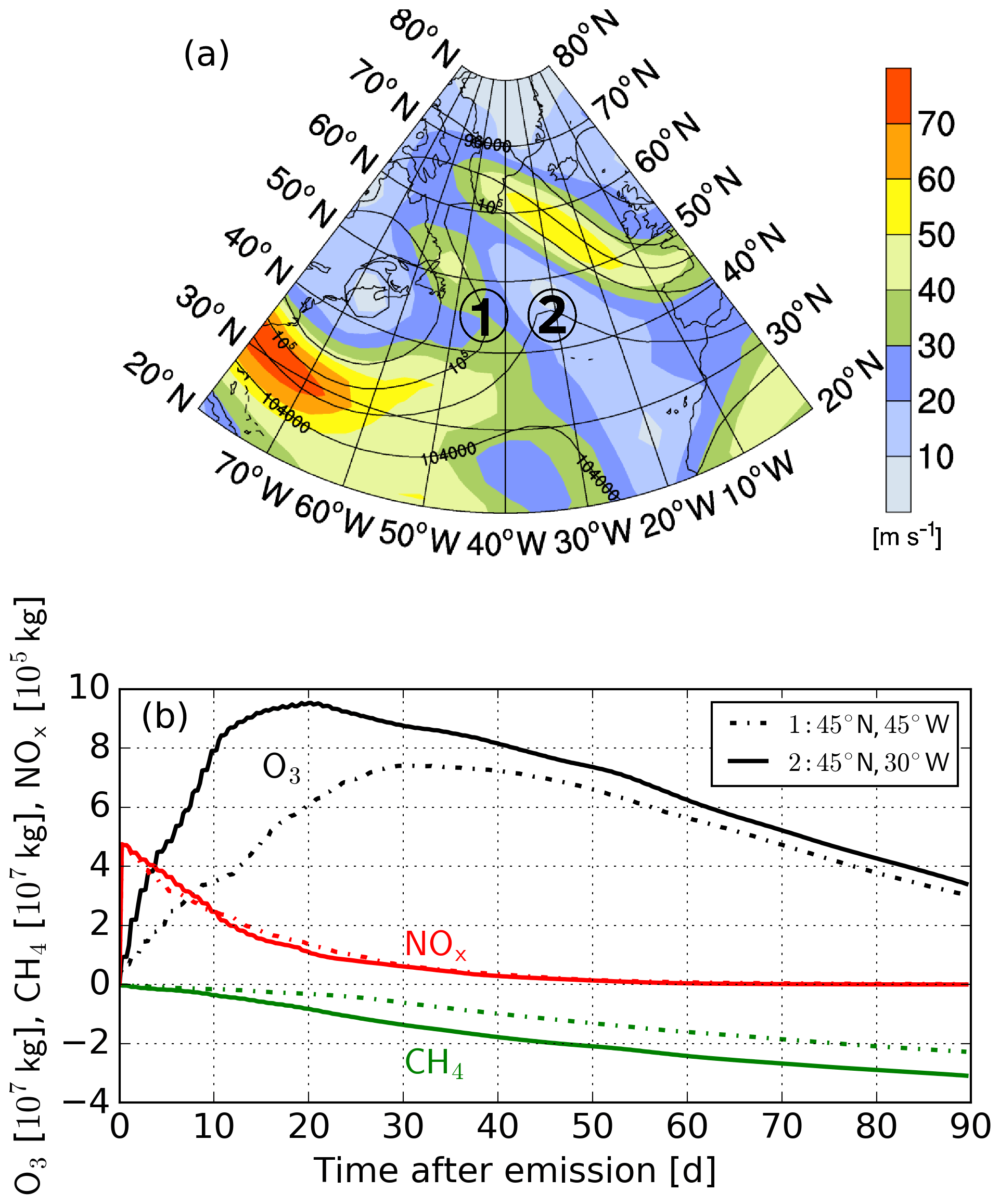
Figure 1(a) Weather conditions at time of emission represented by geopotential height (black contours in gpm) and wind velocities (see colour bar, in m s−1) at 250 hPa. (b) The global composition changes in O3 and CH4 induced by the emitted NOx at two emission locations.
Table 1The integrated O3 and CH4 contribution to atmospheric concentration for both locations given in Fig. 1. The first location (45∘ N 45∘ W) is west of and the second location (45∘ N 30∘ W) within a high-pressure ridge. Additionally, the resulting climate impact for both locations, represented by climate change functions (CCFs), is given. For further details on the climate impact, see Frömming et al. (2020). Integrals are given in kg d−1 and CCF values are given in K kg(N)−1.
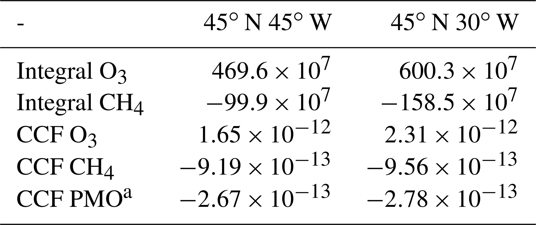
a Primary mode ozone (PMO).
Figure 1b shows the “typical” temporal development of O3 and CH4 due to an aviation-attributed NOx emission for two emission locations next to each other (45∘ N 45∘ W and 45∘ N 30∘ W), representative for the examples presented in Grewe et al. (2017a) and Frömming et al. (2020). Here, one emission region is inside, and the other one is west of a high-pressure ridge (see Fig. 1a). While the emitted NOx decreases in both air parcels, the O3 concentration increases due to the described production processes (Reactions R1–R3). Additionally, the emitted NOx leads to an elimination of HOx by forming nitric acid (HNO3) and peroxynitric acid (HNO4).
Both HNO3 and HNO4 are subsequently removed by heterogeneous or other reactions, leading to an exponential decay of NOx and a complete elimination after about a month. When the NOx mixing ratio is below a certain level, only a little O3 is produced, and loss terms dominate the O3 chemistry, leading to a continuous decrease in the formed O3. At the same time, the additional O3 and NOx form OH, which leads to a depletion of CH4 (Reaction R4). After all NOx and O3 is lost, the negative CH4 anomaly starts to decay and will later reach its original values (not seen in Fig. 1b). For the two emission regions, the resulting O3 gain differs, with the emission region in the high-pressure system having an earlier O3 maximum with a higher magnitude. In contrast, the CH4 depletion is only characterised by a varying magnitude. This large variability in the NOx–O3–CH4 relation, induced by the same NOx emission, is also presented in Fig. 9 of Grewe et al. (2014b). However, the question remains whether the different resulting characteristics for both emission locations given in Fig. 1 can be explained by the different weather conditions experienced by each air parcel.
Within the present study, we investigate the impact of weather situations on changes in O3 and CH4 concentrations induced by NOx emissions in the upper troposphere of the North Atlantic flight sector. In general, it is common to analyse the integrated O3 change or the integrated radiative forcing induced by changes in O3. Table 1 gives the integrated O3 and CH4 for both regions presented in Fig. 1. Additionally, the so-called climate change functions (CCFs), a measure on how the Earth's surface temperature will change due to a locally restricted NOx emission (for more details, see Grewe et al., 2014b, a, and Frömming et al., 2020), is given. The intention of this paper is not to identify correlations between weather conditions and the resulting climate impact. Still, understanding the relation between the resulting climate impact and typical characteristics of the contribution to O3 and CH4 provides valuable insights. An earlier and larger O3 contribution correlates with a higher integrated O3 concentration and a higher resulting climate impact. Analysing the integrated O3 and CH4 is not feasible when analysing the influence of weather conditions on the induced composition changes due to aviation-attributed NOx emissions. Comparing varying weather conditions to a single data point (e.g. the integrated O3) is difficult. For instance, a higher statistical significance is expected when analysing the mean value of a typical weather condition over a 20 d mean until the O3 maximum is reached (for location 2 in Fig. 1 and Table 1) instead of the complete 90 d period, due to the chaotic nature of weather conditions. Thus, typical characteristics of the temporal development of O3 and CH4 are more suitable for this analysis since it is expected that they are directly influenced by varying weather conditions. Therefore, we focus especially on how weather conditions influence the time when the O3 maximum occurs, the total O3 gained, and the total CH4 depleted. Our findings are additionally analysed with respect to inter-seasonal variability. This is achieved by using the results of simulations performed in the European project REACT4C (Reducing Emissions from Aviation by Changing Trajectories for the benefit of Climate, https://www.react4c.eu/ (last access: 16 October 2020) Matthes, 2011). The modelling approach of REACT4C and the methodology used in this study are elaborated in Sect. 2. Following this, all findings of this study will be presented (Sect. 3). In Sect. 4, uncertainties and findings of this study will be discussed, including a possible implementation strategy.
Our analysis of the general concept of REACT4C and the modelling approach used will first be elaborated in order to show how the impacts of NOx emissions on O3 and CH4 were simulated. The idea of the project is presented by Matthes (2011) and Matthes et al. (2012). A complete description of the modelling approach used is given by Grewe et al. (2014b). Afterwards, a detailed description of the steps taken within the analysis of this work is presented.
2.1 REACT4C
REACT4C investigated the feasibility of adapting flight routes and flight altitudes to minimise the climate impact of aviation and to estimate the global effect of such air traffic management (ATM) measures (Grewe et al., 2014b). In this particular study, this mitigation option was tested over the North Atlantic region. The general steps in this modelling approach were as follows: (1) select representative weather patterns; (2) define time-regions; (3) model atmospheric contributions for additional emissions in these time-regions; (4) calculate the adjusted radiative forcing (RF); (5) calculate the climate change function (CCF) for each emission species and induced cloudiness; (6) optimise aircraft trajectories, based on the CCF results, by using an air traffic simulation system (System for traffic Assignment and Analysis at a Macroscopic level, SAAM), which is coupled to an emission tool (Advanced Emission Model, AEM); and (7) calculate the resulting operation costs and the resulting climate impact reduction. For the present study, only steps 1–3 are important and will be further elaborated.
Irvine et al. (2013) identified that by simulating frequently occurring weather situations within a season, the global seasonal impact can be estimated. They analysed meteorological reanalysis data for 21 years for summer and winter. This reanalysis leads to three distinct summer (SP1–3) and five winter (WP1–5) patterns. The different weather patterns mainly vary in their location, orientation and strength of the jet stream, and the phase of the North Atlantic Oscillation and the Arctic Oscillation. A graphical representation of each defined weather pattern is given by Irvine et al. (2013, Figs. 7 and 8 for winter and summer, respectively), and the actual weather situations simulated in REACT4C are presented in Frömming et al. (2020). Due to the lower variability of the jet stream in summer, only three distinct weather situations were determined. The summer patterns occur 19 (SP1), 55 (SP2), and 18 (SP3) times per season and the winter patterns occur 17 (WP1 and WP2), 15 (WP3 and WP4), and 26 (WP5) times per season in the reanalysis data (Irvine et al., 2013). Analogously, REACT4C simulated 8 distinct model days, each representing one of these weather patterns.
To calculate the climate change functions, a time-region grid was defined in the North Atlantic region for seven latitudes (between 30 and 80∘ N) and six longitudes (between 80 and 0∘ W) over four different pressure levels (200, 250, 300, and 400 hPa) to account for different flight levels. At each time-region grid point, unit emissions of CO2, NOx, and H2O are initialised on 50 trajectories at 06:00, 12:00, and 18:00 UTC. However, Grewe et al. (2014b) found that the results show only minor sensitivity with respect to the temporal resolution. Therefore, only 12:00 UTC is considered in this study. The 50 trajectories are randomly located in the respective model grid box in which the specific time-region grid point is located. At each time-region grid point, 5×10⁵ kg of NO (equal to 2.33×10⁵ kg(N)) is emitted, which is then equally distributed onto the trajectories (Grewe et al., 2014b).
2.2 Base model description
The ECHAM/MESSy Atmospheric Chemistry (EMAC) model is a numerical chemistry and climate simulation system that includes sub-models describing tropospheric and middle atmosphere processes and their interaction with ocean, land, and human influences (Jöckel et al., 2010). It uses the second version of the Modular Earth Submodel System (MESSy2) to link multi-institutional computer codes. The core atmospheric model is the fifth-generation European Centre Hamburg general circulation model (ECHAM5, Roeckner et al., 2003). For the present study, we applied EMAC (ECHAM5 version 5.3.02, MESSy version 2.52.0) in the T42L41 resolution, i.e. with a spherical truncation of T42 (corresponding to a quadratic Gaussian grid of approximately 2.8 by 2.8∘ in latitude and longitude) with 41 vertical hybrid pressure levels up to 5 hPa.
The applied model setup comprised multiple MESSy submodules important for the performed simulations. Each of the tracers (i.e. NOx and H2O) is emitted in an air parcel by the submodel TREXP (Tracer Release EXperiments from Point sources). The air parcel is then advected by the submodel ATTILA (Atmospheric Tracer Transport In a LAgrangian model, Reithmeier and Sausen, 2002) using the wind field from EMAC. In addition to the 50 air parcels with tracer loading starting at each time-region, empty background air parcels are modelled in the Northern Hemisphere to allow for additional mixing, which in total yields about 169 000 air parcels. The air parcels have a constant mass, and the mixing ratio of each species is defined on the parcels' centroid. The centroid is assumed to be representative for the whole air parcel and the Lagrangian cells are considered isolated air parcels. While ATTILA is non-diffusive per se, inter-parcel mixing is parameterised by bringing the mass mixing ratio in a parcel closer to the average background mixing ratio, which is the average mixing ratio of all parcels within a grid box. The vertical transport due to subgrid-scale convection in ATTILA is calculated in three steps: (1) mapping the ATTILA tracer concentrations from the air parcels to the EMAC grid, (2) calculating the convective mass fluxes similarly as for standard EMAC tracers, and (3) mapping the calculated tendencies back to the air parcels. While a gain of tracer mass is distributed evenly among the air parcels in a grid cell, a reduction of tracer mass is calculated according to the mass available. Further details are given in Reithmeier and Sausen (2002).
For each trajectory, the contribution of the emission (i.e. NOx and H2O) to the atmospheric concentration of CH4, O3, HNO3, H2O, and OH is calculated over a time period of 90 d by using the submodel AIRTRAC (version 1.0, Frömming et al., 2013; see the Supplement to Grewe et al., 2014b). The tagging approach used by AIRTRAC was first described by Grewe et al. (2010). In this approach, each important chemical reaction is doubled. The first reaction applies to the whole atmosphere (from here onwards referred to as background) and the second only to the additionally emitted tracer (from here onwards referred to as foreground). The submodel MECCA (Module Efficiently Calculating the Chemistry of the Atmosphere) is used to model the background chemical processes in the troposphere and stratosphere. The chemical mechanism used by MECCA can be grouped into sulfur, non-CH4 hydrocarbon, basic O3, CH4, HOx and NOx, and halogen chemistry (Sander et al., 2005). AIRTRAC, on the other hand, calculates the resulting changes due to the additional emitted NOx in the foreground. AIRTRAC assumes that each concentration change of O3 due to aviation is attributed to the emitted NOx, which is consistent with Brasseur et al. (1998). Concentration changes due to additionally emitted NOx are calculated based on the concentration of all chemical species involved in the general chemical system and the concentrations due to the extra emitted NOx. The actual concentration change is then calculated based on the background reaction rate and the fraction of foreground and background concentrations of all reactants (Grewe et al., 2010). In detail, the foreground loss of O3 () via Reaction (R7) is based on the foreground and background concentrations of NO2 and O3 (, and , for foreground and background, respectively) and the background loss of O3 (), as given in Eq. (1).
In total, AIRTRAC calculates the mass development of NOx, O3, HNO3, OH, HO2, and H2O by tracking 14 reactions and reaction groups. These can be split into (1) one group for both the production and the destruction of O3, (2) one reaction for the formation of HNO3, (3) three and five reactions for the OH production and destruction, respectively, and (4) three reaction groups for the production and destruction of HO2. Further, loss processes like wash-out and deposition are taken into account (Grewe et al., 2014b). The results of this mechanism agree well with earlier studies with respect to the regionally different chemical regimes and the overall effect of aviation emissions (Grewe et al., 2017c, Sect. 4.3, therein). The tagging mechanism also enables the quantification of CH4 losses due to the two major reaction pathways, the change in HOx partitioning towards OH due to a NOx emission, and the production of OH due to an enhanced O3 concentration (Grewe et al., 2017c, Fig. 8). Section 4 includes an elaborate discussion on the modelling approach used.
2.3 Analysis performed in this study
Within this study we used the simulation output created by the REACT4C project. As some output variables were not available for all emission locations and weather patterns, not all time-regions and weather patterns could be included in the present study. Some of the raw data of WP2 were subject to data loss and not all analyses could be performed with this weather pattern. Therefore, WP2 has been excluded from the analysis. From 1344 original emission locations, 1115 are analysed. At each emission location all 50 air parcels are taken into account, resulting in 55 750 trajectories being analysed. An output resolution of 6 h was used over 90 d.
The variables taken into account can be categorised into three different groups: (1) background and foreground chemical concentrations, (2) background and foreground chemical reaction rates, and (3) general weather information. All foreground variables are present on the tracer grid, whereas background data are stored on the original EMAC grid. To simplify the analysis, background data were re-gridded onto the tracer grid. Here, it has been assumed that all background data within a grid box are valid for each air parcel within this specific EMAC grid box.
Due to the general complexity of the atmospheric chemistry, many variables can potentially influence changes in O3 and CH4 concentrations induced by NOx emissions. Therefore, correlation matrices were used to identify interacting parameters. For these matrices the three most common statistical measures to identify correlations were used (Pearson, Kendall, and Spearman's rank correlation coefficient). Statistical significance is ensured by using t tests, one-way analysis of variance (ANOVA), and Tukey’s honest significant difference (HSD) tests.
The long-term reduction of O3 due to the induced CH4 loss (i.e. PMO) occurs far beyond the 90 d simulated by REACT4C. Simulating the effect of PMO explicitly is computationally too expensive for the modelling approach used. In REACT4C, PMO was thus not modelled explicitly. Instead a constant scaling factor of 0.29, based on Dahlmann (2012), was applied to the resulting climate impact of CH4 (Grewe et al., 2014b). The effect of PMO is therefore not considered in this study and focus is only on the total CH4 depletion.
Within this section, the results of this study are described. First, a short analysis of the characteristics of the variability in the O3 maximum is presented. The influence of transport processes on the time of the O3 maximum is analysed in Sect. 3.2. The mechanisms controlling total O3 gained are investigated in Sect. 3.3. The influence of tropospheric water vapour on total CH4 depletion is discussed in Sect. 3.4. All findings are presented for summer and winter. An inter-seasonal variability analysis is performed in Sect. 3.5.
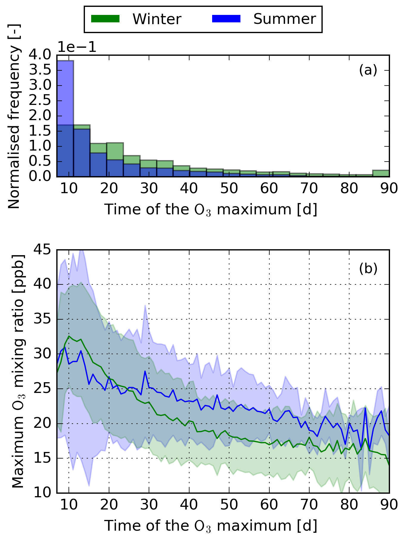
Figure 2(a) Normalised histogram of frequencies when the O3 maximum is reached after emission. Results are normalised to the total number of air parcels in summer and winter, respectively. (b) Mean (solid line) and standard deviation (shaded area) of the maximum O3 mixing ratio in relation to the time when the O3 maximum is reached.
3.1 Characteristics of the temporal development of O3
Figure 2 shows the maximum O3 mixing ratio in relation to the time after emission when the maximum occurs. During winter and summer, high concentration changes are only possible if the O3 maximum occurs early. In this scope, the O3 maximum is defined as the maximum mixing ratio after which no further increase of O3 occurs. Figure 3 shows the “typical” temporal development of O3 for an early, a middle, and a late O3 maximum. The early maximum is characterised by a high production of O3 in the first days after emission. The middle and late maxima are dominated by a slower O3 production. In the case of the late maxima, the extremely slow O3 production leads to a stretched version of the temporal development of the air parcels that have an early or a middle maximum. As stated in Sect. 1, only the early maximum is characterised by a high O3 maximum and the magnitude decreases by one-third and two-thirds for the middle and late maxima, respectively. Figure 2a gives the frequency of when the maximum occurs for both seasons. About 47.5 % and 72 % of all air parcels reach their O3 maximum during the first 21 d in winter and summer, respectively. Only a small number of air parcels do not have defined maxima within the 90 d of simulation (winter: 2.5 %; summer: <1 %). At the end of the simulation period, the O3 concentration of these air parcels is still increasing. However, almost all NOx is removed at the end of simulation. It is thus expected that the formed O3 would be quickly reduced if the simulation was continued beyond the 90 d of simulation. All of these air parcels are emitted at higher altitudes (200 or 250 hPa) and higher latitudes (more than 70 % are emitted north of 50∘ N). During winter, these air parcels are transported to latitudes north of 70∘ N and do not experience any solar radiation (i.e. polar night). The missing solar radiation dampens the O3 formation, leading to no distinct O3 maximum within the 90 simulated days.
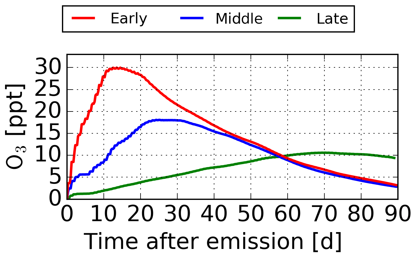
Figure 3“Typical” temporal development of an early (red), a middle (blue) and a late (green) O3 maximum.
3.2 Importance of transport processes on the time of the O3 maxima
It is well established that the O3 production efficiency depends on the general chemical activity and is controlled by weather conditions (i.e. temperature) and the concentration of each reactant. These weather conditions and reactant concentrations differ significantly across the troposphere, such that certain regions have a higher O3 production efficiency. Therefore, the transport into these regions controls the O3 gained. Our analysis shows that air parcels with an early maximum are characterised by a strong downward wind component, whereas late maxima have a weak downward or even an upward vertical wind component (not shown). Therefore, air parcels with an early O3 maximum are those that are transported to lower latitudes (Fig. 4a) and lower altitudes (Fig. 4b). Air parcels with a late maximum mostly stay at the emission altitude and latitude or are transported to higher altitudes and latitudes. For all winter patterns, most maxima occur in a region spanning from 15 to 35∘ N at pressure altitudes between 900 to 600 hPa. The maximum region is slightly shifted to higher altitudes for all summer patterns. No maximum occurs at high latitudes during winter due to the absence of solar radiation in the polar region. This indicates that a significant O3 production, leading to an early O3 maximum, is only possible if an air parcel is transported to lower altitudes and latitudes.
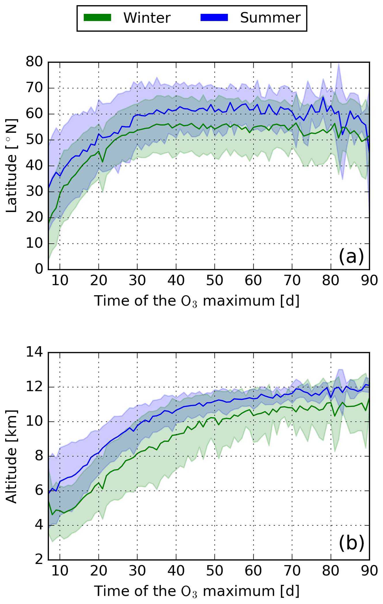
Figure 4Mean (solid line) and standard deviation (shaded area) of the location of each air parcel within the first 7 d after emission in relation to when the maximum O3 mixing ratio is reached (a latitude, b altitude).
Tropospheric vertical transport processes have many causes, e.g. temperature differences, incoming solar radiation, and latent and sensible heat fluxes. Vertical transport occurs in conveyor belt events and causes an exchange of trace gases between the upper and the lower troposphere. Figure 5a shows the mean 250 hPa geopotential height anomaly. The geopotential height is an approximation of the actual height of a pressure surface (here 250 hPa) above the mean sea level. Here, the anomaly is presented for a better comparison of summer and winter, due to generally higher geopotential heights during summer. The anomaly is obtained by deducting the seasonal mean. In classical weather analysis, the geopotential height is used to identify synoptic weather systems. The positive deviation in the geopotential height for air parcels with an early maximum indicates that these air parcels originate from or are transported into and stay within a high-pressure system. Air parcels originating from the core of a high-pressure system have generally earlier maxima compared to air parcels which are transported into high-pressure systems after emission (not shown). It is well known that subsidence dominates vertical transport processes within high-pressure systems, explaining the strong downward motion of air parcels, characterised by early maxima. Air parcels with late maxima stay within low-pressure systems where upward motion dominates.
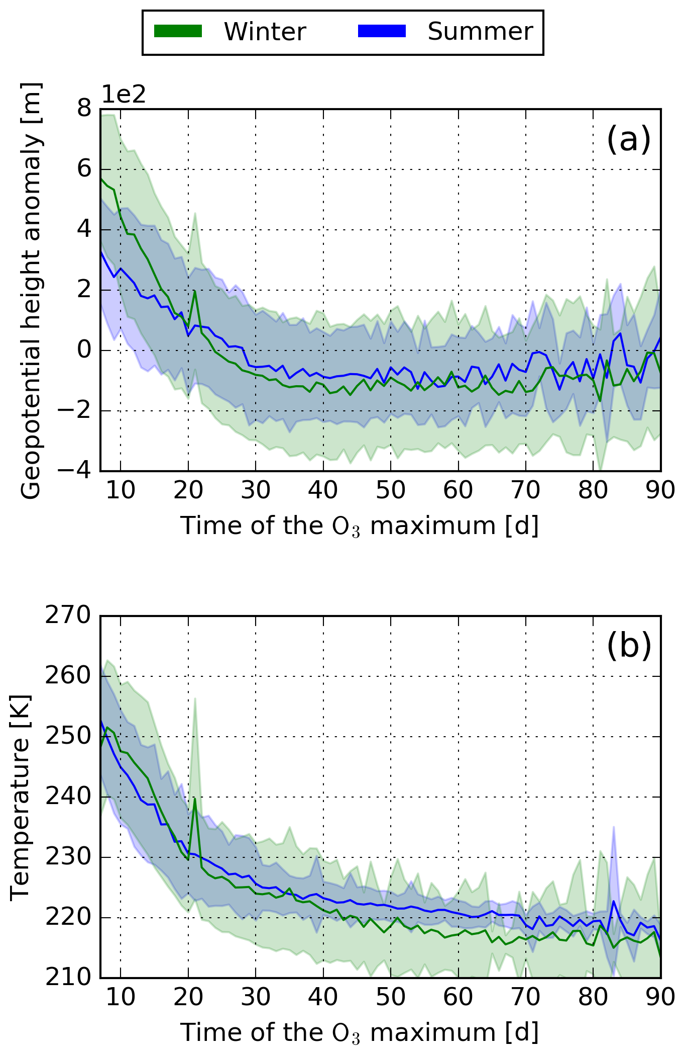
Figure 5(a) Mean 250 hPa geopotential height anomaly. The mean is calculated for the first 7 d after emission, similar to the mean values given in Fig. 4. The anomaly is calculated based on the seasonal mean. (b) Mean dry air temperature. Here, the mean is calculated based on the time between emission and the O3 maximum. Both parameters are given in relation to the time of the O3 maximum. The seasonal mean is represented by the solid line and the standard deviation as shaded area.
3.3 Weather conditions controlling the O3 production efficiency
Even though early O3 maxima are characterised by strong vertical downward transport, transport processes do not directly influence chemical processes in the atmosphere. Temperature is known to be a major factor controlling chemical processes in the atmosphere and is generally higher at lower altitudes and latitudes. Figure 5b shows the mean dry air temperature along the air parcel trajectory until the O3 maximum is reached. The mean dry air temperature is higher for air parcels with early O3 maxima, which is due to the downward and southward transport (leading to higher temperatures) within high-pressure systems. These higher temperatures lead to higher background chemical activity (higher background reaction rates) and therefore accelerate foreground chemistry. Higher temperatures and enhanced photochemical activity at higher altitudes during Northern Hemispheric (NH) summer explain the tendency of earlier maxima in this season.
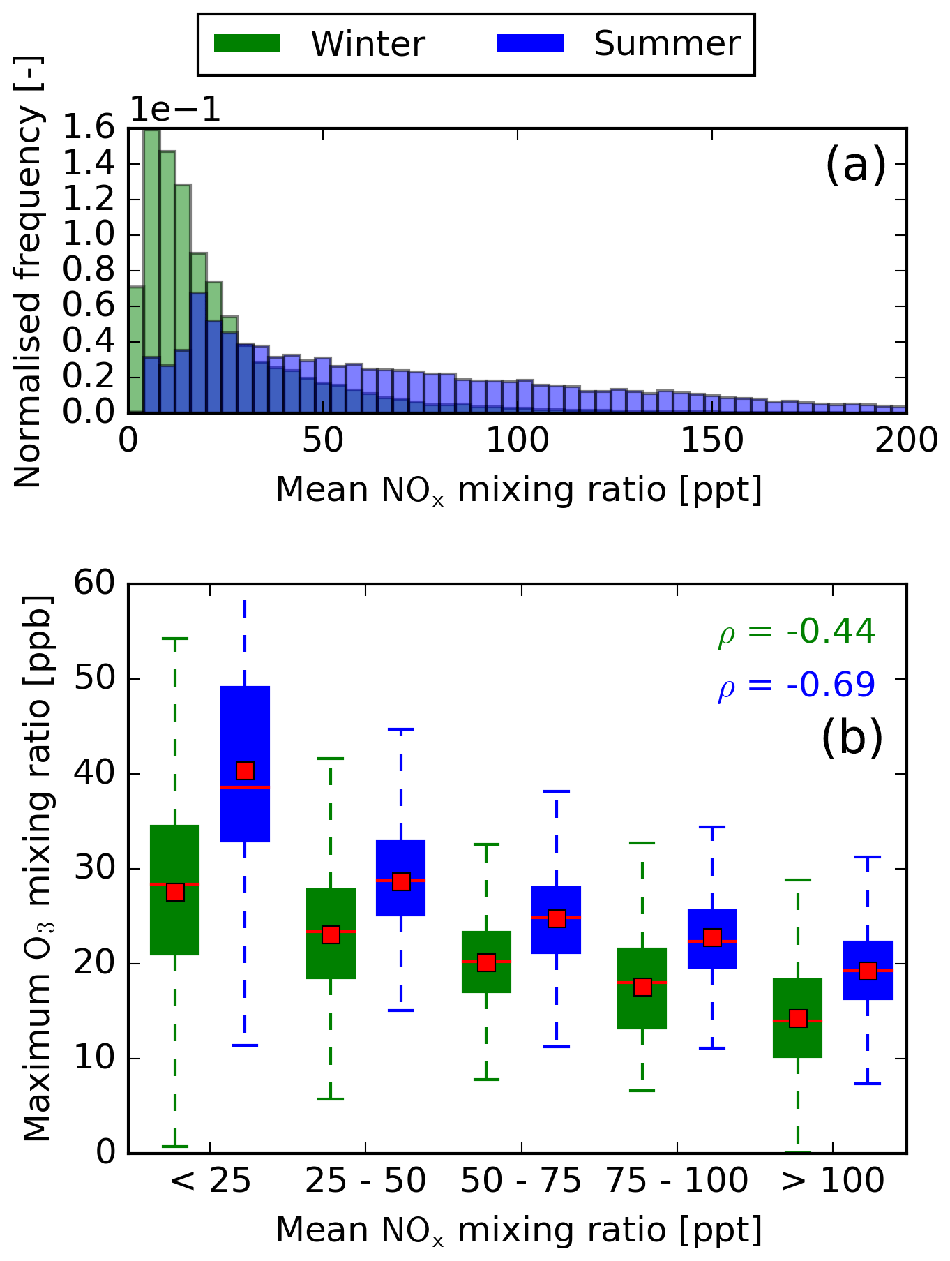
Figure 6(a) Normalised histogram of the mean NOx mixing ratio until the O3 maximum is reached. Results are normalised to the total number of air parcels in summer and winter, respectively. (b) Binned box plots showing the relation between the mean NOx mixing ratio and the magnitude of the O3 maximum. The median and mean for each box plot are represented by red lines and red boxes, respectively. Additionally, the Spearman rank coefficient is given for summer and winter.
From classical chemistry, the efficient production of O3 not only depends on high chemical activity due to higher temperatures but also on the concentrations of the reactants involved. In the case of the formation of O3 due to NOx, these are NO and HO2 (Reaction R1). Figures 6b and 7b show how the mixing ratios of NOx and HOx, respectively, relate to the maximum O3 mixing ratio. Here, NOx and HOx are used to account for the rapid cycling of the species within each radical group. For both seasons, only low NOx concentrations will lead to high O3 contributions. The production of O3 via Reactions (R1) to (R3) dominates at low background NOx concentrations, whereas at high background concentrations, NO2 is eliminated by reacting with OH and HO2, forming HNO3 and HNO4, respectively. From Fig. 7b it becomes evident that a high increase in O3 is only possible at high HOx concentrations, since at low HO2 no O3 will be formed via Reaction (R1).
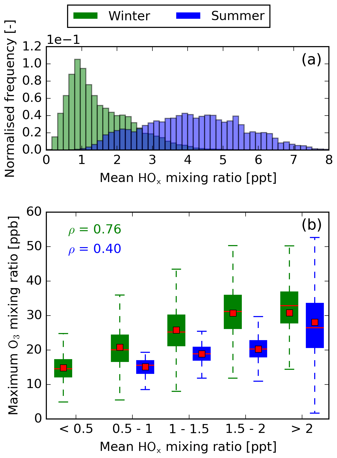
Figure 7(a) Normalised histogram of the mean HOx mixing ratio until the O3 maximum is reached. Results are normalised to the total number of air parcels in summer and winter, respectively. (b) Binned box plots showing the relation between the mean HOx mixing ratio and the magnitude of the O3 maximum. Please note that during summer HOx mixing ratios below 0.5 ppt show no statistical significance. Therefore, no box plot is provided in this case. The median and mean for each box plot are represented by red lines and red boxes, respectively. Additionally, the Spearman rank coefficient is given for summer and winter.
In the upper troposphere, the background NOx concentration is altitude dependent and generally increases towards the tropopause (not shown). On the other hand, HOx is high at low altitudes and latitudes and decreases towards the tropopause. Air parcels with a fast downward transport generally experience lower mean background NOx concentrations and higher HOx background concentrations, resulting in a higher O3 gain. Air parcels that stay close to the tropopause or are even transported into the stratosphere, experience a high background NOx concentration, leading to a lower O3 formation since most NOx is eliminated by forming HNO3 and HNO4. In addition, high background HOx concentrations dominate in high-pressure systems (not shown) explaining why air parcels in high-pressure systems have a generally higher O3 formation.
Summer and winter significantly differ with regard to the correlation of NOx and HOx with the O3 maximum, respectively. Summer has a high Spearman rank coefficient for NOx () but only correlates weakly with HOx (ρ=0.40). Winter, on the other hand, correlates well with HOx (ρ=0.76) but weakly with NOx (). This difference is explained by varying NOx and HOx concentrations in both seasons. Figures 6a and 7a give the normalised frequencies of NOx and HOx for both seasons. It becomes evident that winter is characterised by low NOx and HOx concentrations, whereas summer is dominated by high NOx and HOx concentrations. For many air parcels during summer, enough HOx is available to allow a high formation of O3, but a higher NOx concentration limits the formation of O3 and leads to the formation of HNO3 and HNO4. During winter, the low NOx concentrations theoretically allow for a high O3 formation, but low HOx concentrations limit the efficient production of O3.
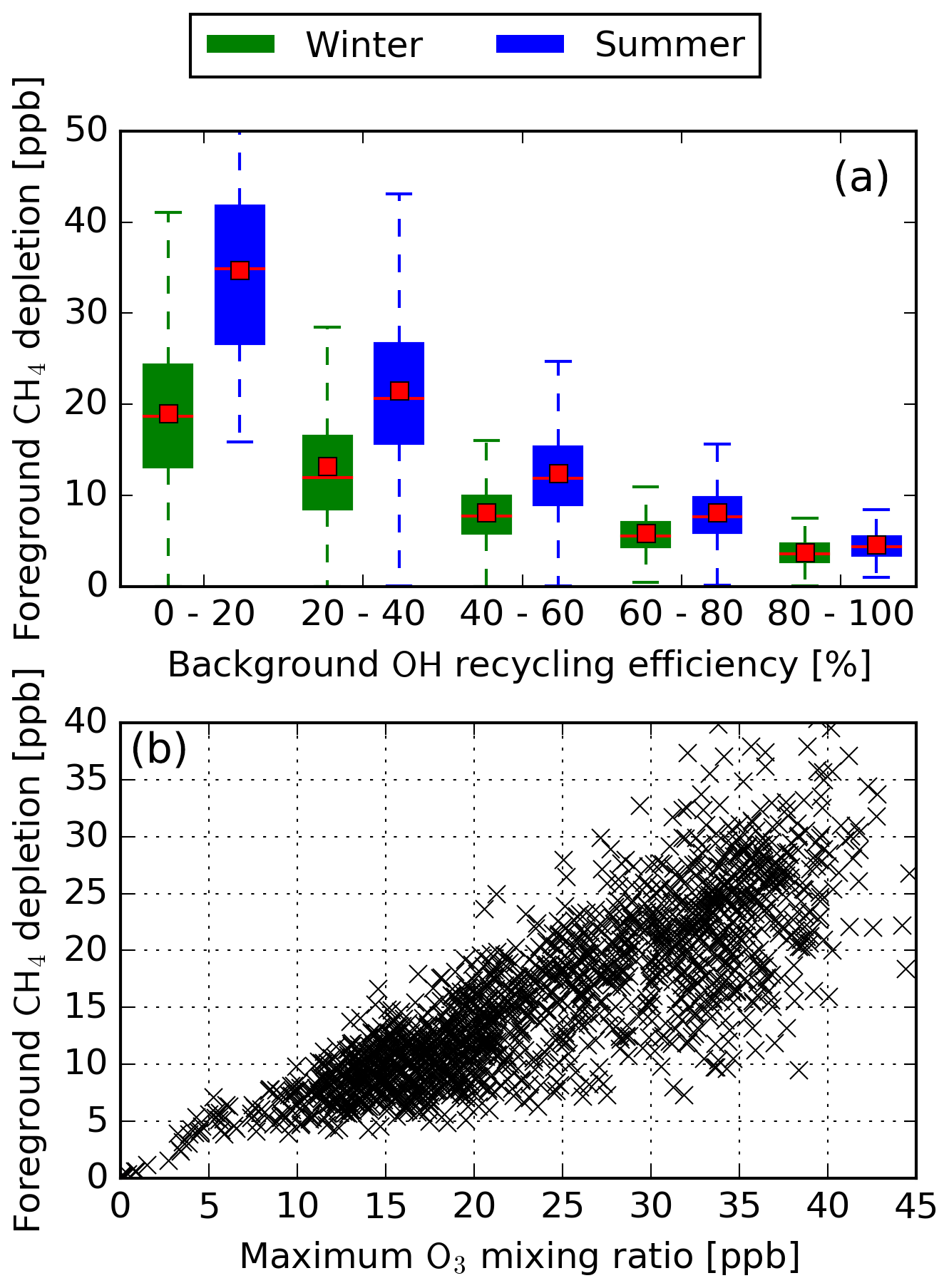
Figure 8(a) Binned box plots of the OH recycling probability. The median and mean for each box plot are represented by red lines and red boxes, respectively. (b) Maximum O3 mixing ratio vs. maximum CH4 mixing ratio for recycling probabilities below 20 % for WP1.
3.4 Influence of water vapour on the total CH4 depletion
In comparison to O3, only the total CH4 depletion is of interest due to its longer atmospheric lifetime. A high O3 concentration leads to a high CH4 depletion (Spearman rank coefficient of 0.66), since O3 is a major source of OH accelerating the depletion of CH4 (Reaction R4). However, the moderate Spearman rank coefficient indicates that other factors additionally control the CH4 depletion process. Our results show that a high foreground CH4 depletion is only possible if the background OH concentration is high. When looking at OH, the fast cycling between OH and HO2 has to be taken into account. Analysing the recycling probability (r) of OH is useful to account for this cycling. Here, we define the recycling probability following Lelieveld et al. (2002):
in which P is the primary production of OH via
and G is the gross OH production when additionally considering the secondary production of OH. In general, when r approaches 100 % the formation of OH becomes autocatalytic. When r approaches 0 %, all OH is formed via Reaction (R8). Based on a perturbation study, Lelieveld et al. (2002) identified that, for recycling probabilities above 60 %, the chemical system becomes buffered and that NOx perturbations in this regime have little impact on OH. Figure 8a shows that a high CH4 depletion is only possible if the recycling probability of background OH is below 60 %. When the major source of OH is from Reaction (R8) (r approaches 0 %), the formed OH is not recycled via NOx, accelerating the depletion of CH4. The major source of foreground OH is the formed O3. A high background OH recycling probability does not necessarily mean that foreground O3 is efficiently produced. The foreground formation of O3 is limited by background NOx and HOx during summer and winter, respectively. Figure 8b shows the relation between the total CH4 depletion and the O3 magnitude for recycling probabilities below 20 % (leftmost box plot in Fig. 8a). Thus, the possible low O3 formed limits the CH4 depletion at low OH recycling probabilities, explaining the high spread in the total CH4 depletion in that regime. It can thus be concluded that a high depletion of CH4 is only possible if the major formation of OH is due to Reaction (R8).
Globally, Lelieveld et al. (2016) estimate that about 30 % of the tropospheric OH is produced by Reaction (R8). This reaction is limited by the availability of O(1D), formed from the photolysis of O3 and H2O. In this study, the highest CH4 depletion rate occurs in tropical regions close to the surface (between 0 and 20∘ N and below 850 hPa), which are dominated by hot and humid weather conditions. These regions are known to have high HOx concentrations due to active photochemistry and large OH sources and sinks. Here, the contribution of OH being produced by water vapour is highest (Lelieveld et al., 2016). A strong correlation exists between the average specific humidity along the air parcel trajectory and the total depletion of CH4 (mean Spearman rank coefficient of 0.77). In particular, air parcels with a low OH recycling probability and thus a high CH4 depletion are characterised by high specific humidity and high incoming solar radiation. Therefore, a high depletion of CH4 is only possible if the air parcel is transported towards low altitudes and latitudes. The transport into tropical regions occurs mainly due to the subsidence in high-pressure systems (see Sect. 3.2).
Table 2Spearman rank coefficients of all identified relations for each individual weather pattern. All correlation factors related to the time and the maximum O3 mixing ratio are calculated based on mean values for the time span between emission and the time of the O3 maximum. The correlation between the total CH4 depletion and specific humidity is based on the mean between time of emission and the time when the total CH4 depletion is reached.
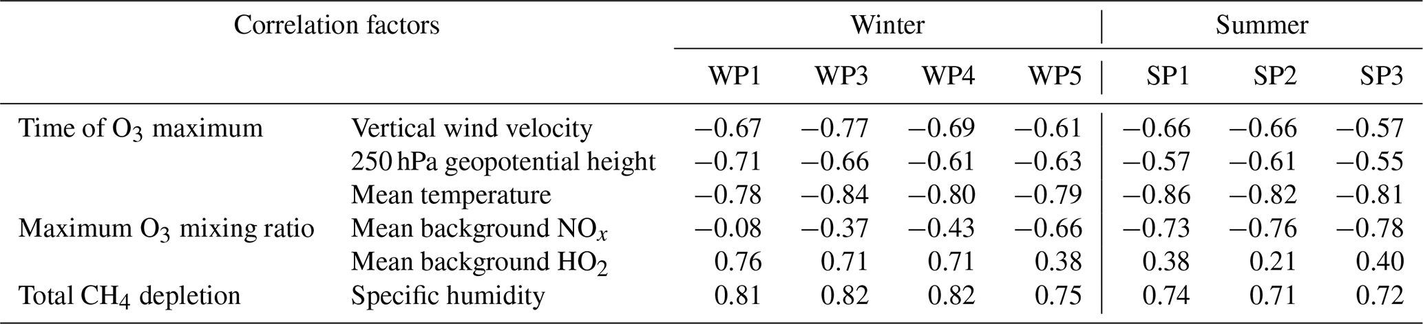

Figure 9Histogram for the mean HOx mixing ratio until the O3 maximum is reached for WP1, WP5, and SP3. Note that mixing ratios above 4 ppt are not shown.
3.5 Inter-seasonal variability
Within this study, specific weather situations (for graphical representations see Irvine et al., 2013, their Figs. 7 and 8, and Frömming et al., 2020) were analysed. Table 2 shows an overview of all correlations analysed within this study for each distinct weather pattern. Vertical transport processes until the O3 maximum, represented by the vertical wind velocity, correlate reasonably well within both seasons. However, during summer the correlation tends to be lower. SP3 has the lowest correlation coefficient and the highest mean downward wind velocity. This pattern is characterised by a high-pressure blocking situation, leading to an overall high layer thickness, resulting in a weaker correlation. It is thus expected that differences in each individual weather situation (i.e. number, location, and strength of the high-pressure systems) cause the inter-seasonal variability. Additionally, downward transport during summer is less important for air parcels to experience high temperatures. This also explains the weaker correlation for the 250 hPa geopotential height during summer. Still, air parcels which stay in a high-pressure region experience earlier maxima during summer.
The mean background concentration of NOx correlates strongly with the O3 magnitude for each SP, giving no indication that there is another parameter that controls the total O3 gain. However, no correlation exists for most WPs. This indicates that in winter, when chemistry is slow at emission locations at middle and higher latitudes, the transport pathway, e.g. towards the tropics, is more important than the chemical background conditions at the time of emission, whereas in summer with active photochemistry, the background NOx concentration plays a dominant role. Only WP5 shows a stronger correlation. At the same time, WP5 has a low correlation with HOx. Figure 9 gives the frequencies of the mean background HOx concentrations for WP1, WP5, and SP3. In comparison to WP1, WP5 is characterised by higher HOx concentrations with most mixing ratios above 1 ppt (WP1 mean: 1.2 ppt, WP5 mean: 1.8 ppt; WP1 median: 0.89 ppt, WP5 median: 1.4 ppt). In general, mixing ratios above 1 ppt allow a high O3 formation (see Fig. 7). This indicates that for most air parcels in WP5, HOx is not the only limiting factor for the O3 gain. At the same time WP5 is characterised by higher NOx mixing ratios (WP1 mean: 18.1 ppt, WP5 mean: 31.6 ppt) explaining the higher correlation with NOx. This indicates that in the case of WP5 the maximum O3 concentration is limited by a combination of HOx and NOx. The chosen example day in EMAC for WP5 occurs at the end of February, whereas the other WPs are initialised in December or early January. This indicates that HOx becomes a less limiting factor towards spring. This suggests that our results are only valid for both analysed seasons and further research is necessary to identify the controlling factors in spring and autumn.
Specific humidity is clearly the controlling factor of the total CH4 depletion for all weather patterns taken into account. Again the correlation is weaker in summer, which is due to the generally higher H2O concentrations. This results in a lower variability in the specific humidity, which weakens the correlation analysed. Here, WP5 again behaves like all SPs. This indicates that O3 and CH4 concentration changes due to emissions in spring are most likely controlled by mechanisms identified for summer.
Our results indicate a large impact of transport patterns on O3 and CH4 concentration changes due to aviation NOx emissions. This is both a highly complex interaction of transport and chemistry, and a relatively small contribution of O3 and CH4 concentration changes against a large natural variability. Hence, a direct validation of our results is not feasible. However, the main processes, such as transport and chemistry can be evaluated individually – at least in parts. In the following paragraphs, we will discuss some aspects of this interaction and the ability of EMAC to reproduce observations.
An important aspect in our study is the model's transport. Short-lived species, which only have a surface source such as 222Radon (222Rn, radioactive decay half-lifetime of 3.8 d), are frequently used to validate fast vertical transport characteristics. Jöckel et al. (2010) and (in more detail) Brinkop and Jöckel (2019) showed that the model is able to capture the 222Rn surface concentrations and vertical profiles, indicating that the vertical transport is well represented in EMAC.
The horizontal transport is difficult to evaluate, and observed trace gases, which resemble the exchange between middle and high latitudes and the tropics, are not available. However, Orbe et al. (2018) compared transport timescales in various global models, e.g. from northern mid-latitudes to the tropics, which differed by 30 %. The inter-hemispheric transport differed by 20 %. The authors concluded that vertical transport is a major source of this variability. More research is needed to better constrain models with respect to their tropospheric transport timescales. A more integrated view on the variability of aviation related transport–chemistry interaction is given by a model intercomparison of NOx concentration differences between a simulation with and without aircraft NOx emissions (Søvde et al., 2014, see their supplementary material). When concentrating only on their winter results to reduce the chemical impact to a minimum, the results clearly show a very similar NOx change in the five models (including EMAC), peaking around 40∘ N at cruise altitude in winter with a tendency to a downward and southward transport to the tropics. However, the peak values vary between 55 and 70 ppt.
Table 3Spearman rank coefficients for the correlation between the vertical transport and the time of the O3 maximum and the specific humidity and the total CH4 loss. Spearman rank coefficients are provided depending on the period used to calculate the mean value. The Spearman rank coefficient for each correlation for the period from the NOx emission until the O3 maximum is also given.

Chemistry (or more specifically the concentrations of chemically active species) is evaluated in detail in Jöckel et al. (2010) and Jöckel et al. (2016). In general, EMAC overestimates the tropospheric O3 column by 5–10 DU in mid-latitudes and 10–15 DU in the tropics. Carbon monoxide, on the other hand, is underestimated, though the variability matches well with observations. The tropospheric oxidation capacity is at the lower end of model estimates but within the models' uncertainty ranges. Jöckel et al. (2016) speculate that lightning NOx emissions or stratosphere-to-troposphere exchange might play a role. It is important to note that variations, which are caused by meteorology are in most cases well represented (e.g. Grewe et al., 2017a, their Sect. 3.2).
Ehhalt and Rohrer (1995) already stated that the net O3 gain strongly depends in a non-linear manner on the NOx mixing ratio. This is generally well reproduced in EMAC (Mertens et al., 2018, Fig. 5) and even by an EMAC predecessor model (Dahlmann et al., 2011; Grewe et al., 2012, their Figs. 4 and 1, respectively). Stevenson et al. (2004) showed the response of O3 and CH4 to a pulse NOx emission, which is very similar to our results (Grewe et al., 2014b, their Fig. 9). Stevenson and Derwent (2009) demonstrated that the NOx concentration at the time of emission strongly defines the resulting climate impact of O3. A similar but weaker relation can be found in the current data set (not shown) (Grewe et al., 2014b, their Fig. 9). For some air parcels the background NOx concentration is low at time of emission, but they are quickly transported to regions characterised by higher concentrations. These air parcels experience a temporal high O3 production shortly after emission due to low NOx concentrations but only little total O3 is formed due to a high mean background NOx mixing ratios after emission. This explains the difference between our correlation and the one of Stevenson and Derwent (2009). Another aspect is the question of how well the REACT4C concept, used to model atmospheric effects of a local emission (Grewe et al., 2014b), represents global modelling approaches, such as Søvde et al. (2014) or Grewe et al. (2017c). The approach was developed to gain more insights into aviation effects that can not conventionally be obtained. Hence, there are by definition limitations in answering this question. However, four indications can be given that support the consistency of the modelling approach. First, the transport scheme is reasonably well established (Brinkop and Jöckel, 2019, and above). Second, the chemical response to a local emission agrees well with earlier findings of Stevenson et al. (2004), who simulated the monthly mean response of O3 and CH4 to a NOx pulse and which are very similar to the results from this approach (Grewe et al., 2014b, their Fig. 9). Third, the use of a trajectory analysis to interpret either observational data or modelling data is well established (Riede et al., 2009; Cooper et al., 2010). Fourth, a first verification of the resulting global pattern of the atmospheric sensitivity to a local NOx emission by comparing it to sparsely available literature data was promising (Yin et al., 2018). This verification is based on a generalisation of the CCFs by developing algorithms to relate the weather information available at the time of emission to the resulting CCF. These algorithmic CCFs (aCCF, van Manen and Grewe, 2019) allow us to predict all weather situations, compared to the limited applicability to a few selected days for the CCFs. An annual climatology of the results from using aCCFs was calculated and compared to conventional approaches by Yin et al. (2018). They conclude that it “shows [that] the variation pattern of the ozone aCCFs matches well with the literature results over the Northern Hemisphere (the latitude between 30 and 90∘ N) and the flight corridor (roughly 9 to 12 km vertical range)”.
From our findings, it can be concluded that the atmospheric conditions at the time of emission are not the only influence on the O3 gain but instead that the region in which the maximum O3 concentration and the maximum concentration change occur also have an influence. The findings of Stevenson and Derwent (2009) are also only valid for summer, and no winter analysis is provided, making it impossible to directly compare our findings identified in Sect. 3.3 to available literature. However, indirectly, by the use of generalised aCCFs, the first findings indicate a reasonably good agreement of the simulated atmospheric response to local NOx emissions.
To conclude, both transport and chemistry processes are crucial for our results. EMAC is in many aspects in line with other model results but has some biases in the concentration of chemical species. However, the variability of chemical species, such as NOx and O3 is better represented than mean values, indicating that the interaction between transport and chemistry is reasonably well simulated. This result should be robust, since our results show a very strong relation between meteorology and the contribution of aviation emission and as this interaction is in principle well represented in EMAC. However, the strength of the O3 response to a NOx emission in a high-pressure system has an uncertainty that we can hardly estimate. Based on the results of the model intercomparison by Søvde et al. (2014), we would expect an uncertainty in the order of 25 %.
The globally increasing aviation activity and the resulting increase in the contribution of aviation to anthropogenic climate change (Lee et al., 2009) result in the necessity for finding possible mitigation strategies (Matthes et al., 2012). One possible mitigation strategy is to reroute flights based on their potential climate impact. The feasibility of this concept was demonstrated by Grewe et al. (2014a, 2017b). However, mitigating the climate impact from aviation by estimating the climate impact and rerouting flight trajectories using the same simulation setup (in resolution, time horizon and chemical mechanism used) as in REACT4C on a day-to-day basis is currently computationally too expensive and not feasible. van Manen and Grewe (2019) and Yin et al. (2018) demonstrated that the CCFs defined in REACT4C can be approximated by algorithms based on meteorological parameters on the day of emission, which significantly reduces the computational demand. The main findings of the present study are a step towards a better understanding of the influence of weather conditions. It allows us to suggest an alternative approach, which is in-between the detailed CCFs of REACT4C and the aCCFs suggested by van Manen and Grewe (2019). All factors identified in the present study provide a correlation to the resulting climate impact but can not be used as a new climate metric. Still, algorithmic CCFs could be defined to estimate the resulting climate impact. This would allow us to use computationally cheaper, entirely dynamic simulations. Two possible weather factors to approximate the resulting climate impact are (1) vertical wind velocity for the impact of O3, and (2) specific humidity for the depletion of CH4. Table 3 gives the Spearman correlation of both factors with the dependence on the simulation time taken into account. It becomes obvious that the correlation is enhanced with the number of days taken into account. Thus, even shorter dynamical simulations would be sufficient for this approximation. The next step would be to develop aCCFs based on the first days after emission. If implemented into general forecasting services, these aCCFs could be used to reroute aviation on a day-to-day basis with low computational demand. However, investigating the feasibility of this approach is beyond the scope of this paper.
The possibility to reduce aviation's climate impact by avoiding climate-sensitive regions heavily depends on our understanding of the driving influences on induced contributions to the chemical composition of the atmosphere. In this study, we demonstrated the importance of transport processes on locally induced aviation-attributed NOx emission on O3 and CH4 concentrations over the North Atlantic flight sector. The induced O3 change is characterised by the time and magnitude of its maximum, and high O3 maxima are only found if the maximum occurs early. Transport processes like subsidence in high-pressure systems lead to early maxima due to the fast transport into regions with a higher chemical activity. In summer, the NOx–HOx relation is limited by background NOx, whereas in winter the limiting factor is low HOx concentrations. When an air parcel is transported into regions with high NOx concentrations in summer, a low change in total O3 occurs, since less O3 is formed in the background. In this case, most NO2 is eliminated by forming HNO3 and HNO4. During winter, low background NOx concentrations allow for a high O3 formation, but due to generally lower HOx concentrations no efficient O3 formation occurs. Air parcels transported quickly towards lower altitudes encounter low NOx but high HOx concentrations, leading to a higher O3 formation, strengthening the importance of transport processes on the O3 formation.
The total depletion of CH4 depends heavily on the background OH concentration. If most OH is formed by its primary formation process, which depends on water vapour, and only a little OH is recycled to HO2, a high depletion of CH4 occurs. Therefore, the water vapour content, which the air parcel experiences along its trajectory, defines the total CH4 depletion. Air parcels transported into lower altitudes and latitudes experience higher water vapour concentrations. Thus, atmospheric transport processes also define the total CH4 depletion. Additionally, only high total O3 gains correlate with a large CH4 depletion.
Due to the complexity of the problem, we are not able to validate our results. It would be challenging to design a measurement campaign to prove the contribution of aviation NOx emissions to O3 and CH4. The standard deviation of background concentrations is generally considered to be higher than changes induced by aviation NOx perturbation, making it hardly detectable (Wauben et al., 1997). Our analysis of the model performance, however, shows that both transport processes and chemical concentrations are reasonably well represented. Our inter-seasonal analysis shows that our findings on the importance of background NOx and HOx concentrations are only valid for the seasons analysed. Due to the high variability of NOx and HOx concentrations in the troposphere, we expect other factors to control the total O3 gain in other regions that were not analysed in this study. Based on the findings of Köhler et al. (2013), we expect our results to be valid for most parts of the northern extratropics. To conclude, further model studies are necessary to fully quantify how transport processes influence induced changes of O3 and CH4 concentrations in all seasons and other regions of interest.
Our results show that transport processes are of the most interest when identifying the impact of local NOx emissions on O3 and CH4. Since entirely dynamic simulations without chemistry are computationally less expensive, the insights gained in this work suggest a more feasible approach wherein the climate impact would be estimated based on transport processes and other weather factors within the first days of simulation. Short-term dynamic simulations would reduce the computational demand and would thus make rerouting flights on a day-to-day basis possible.
The data of the REACT4C project used in this work are archived at the German Climate Computing Centre (Deutsches Klimarechenzentrum, DKRZ) and are available on request.
SR and VG designed the analysis and SR carried it out. CF performed the simulations of REACT4C. SR prepared the manuscript with contributions from all co-authors.
The authors declare that they have no conflict of interest.
This article is part of the special issue “The Modular Earth Submodel System (MESSy) (ACP/GMD inter-journal SI)”. It is not associated with a conference.
This work was supported by the European Union FP7 Project REACT4C (Reducing Emissions from Aviation by Changing Trajectories for the benefit of Climate: https://www.react4c.eu/ (last access: 16 October 2020), grant agreement no. 233772) and contributes to the DLR project Eco2Fly. Computational resources were made available by the German Climate Computing Center (DKRZ) through support from the German Federal Ministry of Education and Research (BMBF) and by the Leibniz-Rechenzentrum (LRZ). We would like to thank Mariano Mertens from DLR for providing an internal review.
This research has been supported by the European Union's Seventh Framework Programme (grant no. 233772).
The article processing charges for this open-access
publication were covered by a Research
Centre of the Helmholtz Association.
This paper was edited by Jason West and reviewed by William Collins and one anonymous referee.
Brasseur, G., Cox, R., Hauglustaine, D., Isaksen, I., Lelieveld, J., Lister, D., Sausen, R., Schumann, U., Wahner, A., and Wiesen, P.: European scientific assessment of the atmospheric effects of aircraft emissions, Atmos. Environ., 32, 2329–2418, https://doi.org/10.1016/S1352-2310(97)00486-X, 1998. a
Brasseur, G. P., Gupta, M., Anderson, B. E., Balasubramanian, S., Barrett, S., Duda, D., Fleming, G., Forster, P. M., Fuglestvedt, J., Gettelman, A., Halthore, R. N., Jacob, S. D., Jacobson, M. Z., Khodayari, A., Liou, K.-N., Lund, M. T., Miake-Lye, R. C., Minnis, P., Olsen, S., Penner, J. E., Prinn, R., Schumann, U., Selkirk, H. B., Sokolov, A., Unger, N., Wolfe, P., Wong, H.-W., Wuebbles, D. W., Yi, B., Yang, P., and Zhou, C.: Impact of Aviation on Climate: FAA’s Aviation Climate Change Research Initiative (ACCRI) Phase II, B. Am. Meteorol. Soc., 97, 561–583, https://doi.org/10.1175/BAMS-D-13-00089.1, 2016. a
Brinkop, S. and Jöckel, P.: ATTILA 4.0: Lagrangian advective and convective transport of passive tracers within the ECHAM5/MESSy (2.53.0) chemistry–climate model, Geosci. Model Dev., 12, 1991–2008, https://doi.org/10.5194/gmd-12-1991-2019, 2019. a, b
Cooper, O. R., Parrish, D. D., Stohl, A., Trainer, M., Nédélec, P., Thouret, V., Cammas, J. P., Oltmans, S. J., Johnson, B. J., Tarasick, D., Leblanc, T., McDermid, I. S., Jaffe, D., Gao, R., Stith, J., Ryerson, T., Aikin, K., Campos, T., Weinheimer, A., and Avery, M. A.: Increasing springtime ozone mixing ratios in the free troposphere over western North America, Nature, 463, 344–348, https://doi.org/10.1038/nature08708, 2010. a
Dahlmann, K.: Eine Methode zur effizienten Bewertung von Maßnahmen zur Klimaoptimierung des Luftverkehrs, Ph.D thesis, Ludwig Maximilians Universität, Munich, Germany, 2012. a
Dahlmann, K., Grewe, V., Ponater, M., and Matthes, S.: Quantifying the contributions of individual NOx sources to the trend in ozone radiative forcing, Atmos. Environ., 45, 2860–2868, https://doi.org/10.1016/j.atmosenv.2011.02.071, 2011. a
Ehhalt, D. and Rohrer, F.: The impact of commercial aircraft on tropospheric ozone, Roy. Soc. Ch., 170, 105–120, 1995. a
Frömming, C., Grewe, V., Brinkop, S., and Jöckel, P.: Documentation of the EMAC submodels AIRTRAC 1.0 and CONTRAIL 1.0, Supplement of Grewe et al.(2014b), 2013. a
Frömming, C., Grewe, V., Brinkop, S., Jöckel, P., Haslerud, A. S., Rosanka, S., van Manen, J., and Matthes, S.: Influence of the actual weather situation on non-CO2 aviation climate effects: The REACT4C Climate Change Functions, Atmos. Chem. Phys. Discuss., https://doi.org/10.5194/acp-2020-529, in review, 2020. a, b, c, d, e, f
Frömming, C., Ponater, M., Dahlmann, K., Grewe, V., Lee, D. S., and Sausen, R.: Aviation-induced radiative forcing and surface temperature change in dependency of the emission altitude, J. Geophys. Res.-Atmos., 117, https://doi.org/10.1029/2012JD018204, 2012. a
Gilmore, C. K., Barrett, S. R. H., Koo, J., and Wang, Q.: Temporal and spatial variability in the aviation NOx-related O3 impact, Environ. Res. Lett., 8, 034 027, https://doi.org/10.1088/1748-9326/8/3/034027, 2013. a
Grewe, V., Tsati, E., and Hoor, P.: On the attribution of contributions of atmospheric trace gases to emissions in atmospheric model applications, Geosci. Model Dev., 3, 487–499, https://doi.org/10.5194/gmd-3-487-2010, 2010. a, b
Grewe, V., Dahlmann, K., Matthes, S., and Steinbrecht, W.: Attributing ozone to NOx emissions: Implications for climate mitigation measures, Atmos. Environ., 59, 102–107, https://doi.org/10.1016/j.atmosenv.2012.05.002, 2012. a
Grewe, V., Champougny, T., Matthes, S., Frömming, C., Brinkop, S., Søvde, O. A., Irvine, E. A., and Halscheidt, L.: Reduction of the air traffic's contribution to climate change: A REACT4C case study, Atmos. Environ., 94, 616–625, https://doi.org/10.1016/j.atmosenv.2014.05.059, 2014a. a, b
Grewe, V., Frömming, C., Matthes, S., Brinkop, S., Ponater, M., Dietmüller, S., Jöckel, P., Garny, H., Tsati, E., Dahlmann, K., Søvde, O. A., Fuglestvedt, J., Berntsen, T. K., Shine, K. P., Irvine, E. A., Champougny, T., and Hullah, P.: Aircraft routing with minimal climate impact: the REACT4C climate cost function modelling approach (V1.0), Geosci. Model Dev., 7, 175–201, https://doi.org/10.5194/gmd-7-175-2014, 2014b. a, b, c, d, e, f, g, h, i, j, k, l, m
Grewe, V., Dahlmann, K., Flink, J., Frömming, C., Ghosh, R., Gierens, K., Heller, R., Hendricks, J., Jöckel, P., Kaufmann, S., Kölker, K., Linke, F., Luchkova, T., Lührs, B., Van Manen, J., Matthes, S., Minikin, A., Niklaß, M., Plohr, M., Righi, M., Rosanka, S., Schmitt, A., Schumann, U., Terekhov, I., Unterstrasser, S., Vázquez-Navarro, M., Voigt, C., Wicke, K., Yamashita, H., Zahn, A., and Ziereis, H.: Mitigating the Climate Impact from Aviation: Achievements and Results of the DLR WeCare Project, Aerospace, 4, 34, https://doi.org/10.3390/aerospace4030034, 2017a. a, b, c, d
Grewe, V., Matthes, S., Frömming, C., Brinkop, S., Jöckel, P., Gierens, K., Champougny, T., Fuglestvedt, J., Haslerud, A., Irvine, E., and Shine, K.: Feasibility of climate-optimized air traffic routing for trans-Atlantic flights, Environ. Res. Lett., 12, 034 003, https://doi.org/10.1088/1748-9326/aa5ba0, 2017b. a
Grewe, V., Tsati, E., Mertens, M., Frömming, C., and Jöckel, P.: Contribution of emissions to concentrations: the TAGGING 1.0 submodel based on the Modular Earth Submodel System (MESSy 2.52), Geosci. Model Dev., 10, 2615–2633, https://doi.org/10.5194/gmd-10-2615-2017, 2017c. a, b, c
Grewe, V., Matthes, S., and Dahlmann, K.: The contribution of aviation NOx emissions to climate change: are we ignoring methodological flaws?, Environ. Res. Lett., 14, 121 003, https://doi.org/10.1088/1748-9326/ab5dd7, 2019. a
Irvine, E. A., Hoskins, B. J., Shine, K. P., Lunnon, R. W., and Froemming, C.: Characterizing North Atlantic weather patterns for climate-optimal aircraft routing, Meteorol. Appl., 20, 80–93, https://doi.org/10.1002/met.1291, 2013. a, b, c, d
Jöckel, P., Kerkweg, A., Pozzer, A., Sander, R., Tost, H., Riede, H., Baumgaertner, A., Gromov, S., and Kern, B.: Development cycle 2 of the Modular Earth Submodel System (MESSy2), Geosci. Model Dev., 3, 717–752, https://doi.org/10.5194/gmd-3-717-2010, 2010. a, b, c
Jöckel, P., Tost, H., Pozzer, A., Kunze, M., Kirner, O., Brenninkmeijer, C. A. M., Brinkop, S., Cai, D. S., Dyroff, C., Eckstein, J., Frank, F., Garny, H., Gottschaldt, K.-D., Graf, P., Grewe, V., Kerkweg, A., Kern, B., Matthes, S., Mertens, M., Meul, S., Neumaier, M., Nützel, M., Oberländer-Hayn, S., Ruhnke, R., Runde, T., Sander, R., Scharffe, D., and Zahn, A.: Earth System Chemistry integrated Modelling (ESCiMo) with the Modular Earth Submodel System (MESSy) version 2.51, Geosci. Model Dev., 9, 1153–1200, https://doi.org/10.5194/gmd-9-1153-2016, 2016. a, b
Kärcher, B.: Formation and radiative forcing of contrail cirrus, Nat. Commun., 9, 1824, https://doi.org/10.1038/s41467-018-04068-0, 2018. a
Köhler, M., Rädel, G., Shine, K., Rogers, H., and Pyle, J.: Latitudinal variation of the effect of aviation NOx emissions on atmospheric ozone and methane and related climate metrics, Atmos. Environ., 64, 1–9, https://doi.org/10.1016/j.atmosenv.2012.09.013, 2013. a, b
Köhler, M. O., Rädel, G., Dessens, O., Shine, K. P., Rogers, H. L., Wild, O., and Pyle, J. A.: Impact of perturbations to nitrogen oxide emissions from global aviation, J. Geophys. Res.-Atmos., 113, D11305, https://doi.org/10.1029/2007JD009140, 2008. a
Lee, D. S., Fahey, D. W., Forster, P. M., Newton, P. J., Wit, R. C., Lim, L. L., Owen, B., and Sausen, R.: Aviation and global climate change in the 21st century, Atmos. Environ., 43, 3520–3537, https://doi.org/10.1016/j.atmosenv.2009.04.024, 2009. a, b, c
Lelieveld, J., Peters, W., Dentener, F. J., and Krol, M. C.: Stability of tropospheric hydroxyl chemistry, J. Geophys. Res.-Atmos., 107, D234715, https://doi.org/10.1029/2002JD002272, 2002. a, b
Lelieveld, J., Gromov, S., Pozzer, A., and Taraborrelli, D.: Global tropospheric hydroxyl distribution, budget and reactivity, Atmos. Chem. Phys., 16, 12477–12493, https://doi.org/10.5194/acp-16-12477-2016, 2016. a, b
Matthes, S.: Climate-optimised flight planning–REACT4C in Innovation for a Sustainable Avation in a Global Environment, in: Proceedings of the Sixth European Aeronautics Days, Madrid, Spain, 30 March–01 April 2011, 122–128, 2011. a, b
Matthes, S., Schumann, U., Grewe, V., Frömming, C., Dahlmann, K., Koch, A., and Mannstein, H.: Climate Optimized Air Transport, Springer, Berlin, Heidelberg, Germany, https://doi.org/10.1007/978-3-642-30183-4_44, 727–746, 2012. a, b
Mertens, M., Grewe, V., Rieger, V. S., and Jöckel, P.: Revisiting the contribution of land transport and shipping emissions to tropospheric ozone, Atmos. Chem. Phys., 18, 5567–5588, https://doi.org/10.5194/acp-18-5567-2018, 2018. a
Orbe, C., Yang, H., Waugh, D. W., Zeng, G., Morgenstern , O., Kinnison, D. E., Lamarque, J.-F., Tilmes, S., Plummer, D. A., Scinocca, J. F., Josse, B., Marecal, V., Jöckel, P., Oman, L. D., Strahan, S. E., Deushi, M., Tanaka, T. Y., Yoshida, K., Akiyoshi, H., Yamashita, Y., Stenke, A., Revell, L., Sukhodolov, T., Rozanov, E., Pitari, G., Visioni, D., Stone, K. A., Schofield, R., and Banerjee, A.: Large-scale tropospheric transport in the Chemistry–Climate Model Initiative (CCMI) simulations, Atmos. Chem. Phys., 18, 7217–7235, https://doi.org/10.5194/acp-18-7217-2018, 2018. a
Reithmeier, C. and Sausen, R.: ATTILA: atmospheric tracer transport in a Lagrangian model, Tellus B, 54, 278–299, https://doi.org/10.1034/j.1600-0889.2002.01236.x, 2002. a
Riede, H., Jöckel, P., and Sander, R.: Quantifying atmospheric transport, chemistry, and mixing using a new trajectory-box model and a global atmospheric-chemistry GCM, Geosci. Model Dev., 2, 267–280, https://doi.org/10.5194/gmd-2-267-2009, 2009. a
Roeckner, E., Bäuml, G., Bonaventura, L., Brokopf, R., Esch, M., Giorgetta, M., Hagemann, S., Kirchner, I., Kornblueh, L., Manzini, E., Rhodin, A., Schlese, U., Schulzweida, U., and Tompkins, A.: The atmospheric general circulation model ECHAM 5. Part I: Model description., Tech. Rep. 349, Max Planck Institute for Meteorology, Hamburg, Germany, 2003. a
Sander, R., Kerkweg, A., Jöckel, P., and Lelieveld, J.: Technical note: The new comprehensive atmospheric chemistry module MECCA, Atmos. Chem. Phys., 5, 445–450, https://doi.org/10.5194/acp-5-445-2005, 2005. a
Shine, K. P., Derwent, R., Wuebbles, D., and Morcrette, J.: Radiative forcing of climate, in: Climate Change: The IPCC Scientific Assessment (1990), Report prepared for Intergovernmental Panel on Climate Change by Working Group I, edited by: Houghton, J. T., Jenkins, G. J., and Ephraums, J. J., Cambridge University Press, Cambridge, Great Britain, New York, NY, USA, and Melbourne, Australia, 41–68, 1990. a
Stevenson, D. S. and Derwent, R. G.: Does the location of aircraft nitrogen oxide emissions affect their climate impact?, Geophys. Res. Lett., 36, L17810, https://doi.org/10.1029/2009GL039422, 2009. a, b, c, d
Stevenson, D. S., Doherty, R. M., Sanderson, M. G., Collins, W. J., Johnson, C. E., and Derwent, R. G.: Radiative forcing from aircraft NOx emissions: Mechanisms and seasonal dependence, J. Geophys. Res.-Atmos, 109, D17307, https://doi.org/10.1029/2004JD004759, 2004. a, b
Søvde, O. A., Matthes, S., Skowron, A., Iachetti, D., Lim, L., Owen, B., Øivind Hodnebrog, Genova, G. D., Pitari, G., Lee, D. S., Myhre, G., and Isaksen, I. S.: Aircraft emission mitigation by changing route altitude: A multi-model estimate of aircraft NOx emission impact on O3 photochemistry, Atmos. Environ., 95, 468–479, https://doi.org/10.1016/j.atmosenv.2014.06.049, 2014. a, b, c
van Manen, J. and Grewe, V.: Algorithmic climate change functions for the use in eco-efficient flight planning, Transport. Res. D-Tr E, 67, 388–405, https://doi.org/10.1016/j.trd.2018.12.016, 2019. a, b, c
Wauben, W., Velthoven, P., and Kelder, H.: A 3D chemistry transport model study of changes in atmospheric ozone due to aircraft NOx emissions, Atmos. Environ., 31, 1819–1836, https://doi.org/10.1016/S1352-2310(96)00332-9, 1997. a
Wild, O., Prather, M. J., and Akimoto, H.: Indirect long-term global radiative cooling from NOx Emissions, Geophys. Res. Lett., 28, 1719–1722, https://doi.org/10.1029/2000GL012573, 2001. a, b
Yin, F., Grewe, V., van Manen, J., Matthes, S., Yamashita, H., Linke, F., and Lührs, B.: Verification of the ozone algorithmic climate change functions for predicting the short-term NOx effects from aviation en-route, in: Proceeding of the 8th International Conference for Research in Air Transportation, Barcelona, Spain, 6–29 June 2018, 1–8, 2018. a, b, c